RRM: Robust Reward Model Training Mitigates Reward Hacking
Abstract
Reward models (RMs) play a pivotal role in aligning large language models (LLMs) with human preferences. However, traditional RM training, which relies on response pairs tied to specific prompts, struggles to disentangle prompt-driven preferences from prompt-independent artifacts, such as response length and format. In this work, we expose a fundamental limitation of current RM training methods, where RMs fail to effectively distinguish between contextual signals and irrelevant artifacts when determining preferences. To address this, we introduce a causal framework that learns preferences independent of these artifacts and propose a novel data augmentation technique designed to eliminate them. Extensive experiments show that our approach successfully filters out undesirable artifacts, yielding a more robust reward model (RRM). Our RRM improves the performance of a pairwise reward model trained on Gemma-2-9b-it, on RewardBench, increasing accuracy from 80.61% to 84.15%. Additionally, we train two DPO policies using both the RM and RRM, demonstrating that the RRM significantly enhances DPO-aligned policies, improving MT-Bench scores from 7.27 to 8.31 and length-controlled win-rates in AlpacaEval-2 from 33.46% to 52.49%.
1 Introduction
Reinforcement Learning from Human Feedback (RLHF) has become a cornerstone in aligning large language models (LLMs) with human preferences to produce responses that are more helpful, honest, and harmless (Ouyang et al., 2022; Bai et al., 2022a). This approach involves training a reward model (RM) on human feedback, which then guides the LLM to generate high-quality responses through reinforcement learning. The success of RLHF is evident in various AI systems, such as Gemini (Team et al., 2023) and GPT-4 (Achiam et al., 2023). Despite its effectiveness, RLHF faces the fundamental issue of reward hacking (Gao et al., 2023), where the model maximizes the reward function without truly aligning with the intended human preferences. This hacking issue occurs because the RM, while a powerful tool, is an imperfect proxy for human judgment and often struggles with out-of-distribution generalization (Eisenstein et al., 2023).
The reward hacking problem manifests in several ways, with verbosity being a common issue: LLMs tend to generate longer responses to appear more detailed or explanatory, exploiting human raters’ bias towards lengthier content (Shen et al., 2023b; Singhal et al., 2023). In recognition of this challenge, extensive efforts have been made in the literature. ODIN (Chen et al., ) designs a two-head approach to learn the quality reward that is orthogonal to length. Similarly, length-controlled Alpaca (Dubois et al., 2024a) estimates the controlled direct effect (VanderWeele, 2011) through logistic regression by adjusting the length. To mitigate the length bias, an improved version (Park et al., 2024) of DPO (Rafailov et al., 2024) introduces length as penalty to the reward score. In practice, there are more reward hacking patterns beyond length, such as format (markdowns, bold-faces) and patterns (certain -grams or emojis). This is largely due to the large output space of language with limited preference data, as well as the diverse and subjective nature of human preferences.
It is challenging to identify and mitigate all potential exploitation patterns. We may consider the causal perspective to explain this phenomena. Given a prompt and a pair of responses , the human preference can be caused by the real quality that is associated with the prompt, or by the context-free artifacts in the responses that do not depend on prompt. Traditional reward model training cannot differentiate the above two factors. There are two reasons for this. First, the pair of responses are always contextual and on-topic to the prompt, thus no counterfactual prompt (prompt from another examples) is used. The reward model may learn the artifacts existing in the responses by ignoring the prompt. If we use the counterfactual prompt, it can help estimate the level of artifact bias ( with ) existing in the preference dataset (Zhao et al., 2021). Second, even if we adjust a few common artifacts, not all artifacts are observable and thus there is no easy way to control all the artifacts explicitly to answer the question “what will the preference be if both responses share the same artifacts?”.
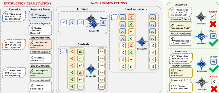
In response to these challenges, we propose a simple and effective method to improve reward modeling. We first formulate the reward model training in a causal framework, then we augment the reward model training data based on the causal rules. By doing so, we can effectively adjust the artifacts and only learn the real quality. Our pipeline is illustrated in Figure 1, where we augment the reward model training data by using responses from other examples to effectively balance the artifacts in chosen and rejected responses. To summarize, the contributions of this paper are three-fold:
-
•
We identify a key issue with traditional reward model training: it often fails to distinguish between genuine contextual preference signals and spurious context-free artifacts.
-
•
To address this, we propose a causal graph for human preference modeling and introduce data augmentation to mitigate artifacts learned by the reward model.
-
•
We further demonstrate that policies trained on these robust reward models consistently outperform those based on baseline reward models.
2 Preliminaries
In preference learning, we assume that there exists a preference oracle that determines the probability that response is preferred over given the prompt . Our goal is to optimize the preference by querying the preference oracle within certain budget constraint. In what follows, we first review the major ways to approximate and estimate the oracle based on a human preference dataset . where represents prompt for example , and represents the chosen and rejected response, respectively.
Reward models
Bradley-Terry pointwise reward model (Bradley & Terry, 1952; Ouyang et al., 2022) is a widely adopted method, which additionally assumes that there exists a reward function and the preference oracle satisfies
Then, we can fit the Bradley-Terry model by maximizing the log-likelihood on the training set:
| (1) |
The second predominant approach is the pairwise ranking model (Zhao et al., 2023; Jiang et al., 2023), which takes a prompt and a pair of responses as the input, and directly predicts the probability , which subsumes the BT model as a subclass. In the literature, the pairwise preference model has shown to outperform pointwise BT reward both empirically (Zhao et al., 2023; Jiang et al., 2023; Dong et al., 2024) and theoretically (Ye et al., 2024) due to its flexibility and larger function class capacity. Specifically, we denote the pairwise ranking model as and leverage the next token prediction ability of the language model to format the sample as:
“[CONTEXT] {} [RESPONSE A] {} [RESPONSE B] {}”
Then, the outputs either “A” or “B” as preferred one. We use the probability of decoding “A” as estimation of the preference probability 111We randomly flip response pairs and associated labels to remove positional bias.. In this work, we use the pairwise ranking model for its superior performance and flexibility.
Alignment Algorithms
Start with a reward function , a reference policy , and input prompt distribution , a policy is trained to optimize for the following objective:
| (2) |
where is the KL penalty coefficient. Several algorithms have been proposed to solve the above optimization, including PPO (Schulman et al., 2017; Ziegler et al., 2019), SLiC (Zhao et al., 2023), DPO (Rafailov et al., 2024), RSO (Liu et al., 2024b), and IPO (Azar et al., 2024). For a stable evaluation process, we use DPO in this work for preference alignment. For a given preference dataset , DPO use the following loss function:
| (3) |
Reward Hacking
Reward model is not perfect due to its limited model size, limited training data, and distribution shift between training data and alignment prompts and responses (Eisenstein et al., 2023; Gao et al., 2023; Guo et al., 2024; Xiong et al., ). Several works have been proposed to mitigate reward hacking. They mainly focus on observable artifacts such as length (Chen et al., ; Dubois et al., 2024a; Shen et al., 2023b). Shen et al. (2023a) propose to enforce the consistency in reward model via data augmentation. Reward hacking can also be mitigated during policy training with post-adjusted reward (Park et al., 2024) or with post-training model merge (Lin et al., 2023). We focus on improving the reward model by addressing reward hacking from a causal perspective.
Causal Inference
Causal inference can be embedded in graphical model frameworks as a directed acyclic graph (DAG) with causal relationship represented as a directed edge (Pearl, 2009; Lee et al., 2020). We say a random vector to be faithful with respect to a DAG if for any , and any subset ,
| (4) |
where denotes and are independent conditional on . The definition of d-separation is as follows: suppose we are given a DAG ; then, for two nodes , a subset of d-connects and if there exists a path between and such that every collider in either belongs to or has a descendent in , and no other node in belongs to . If does not d-connect and , then it d-separates and . See Appendix A.5 for more details.
3 Robust Reward Model Training
3.1 Causal framework
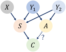
We formulate a DAG to model the causal relationships among different quantities (Figure 2). We assume the distribution of to be faithful to the DAG. is the sufficient statistic (Lehmann & Casella, 2006) that captures the contextual effect that one response fulfills the need of the prompt better than the other. is the sufficient statistic that captures the context-free artifacts that only depend on two responses. Such artifacts can include length, format (bold faces, bullet points, markdown, etc), and certain patterns (-grams such as “Sure, here is the response:”). In traditional reward model training, the model may hack the patterns in . Suppose 80% of winning responses to be longer, then the reward model can get 80% accuracy by just counting the number of tokens. Formally, we construct two hypothesis:
-
•
: there is no causal edge from to .
-
•
: there is a causal edge from to .
Proposition 3.1.
In traditional reward model training, and are not always distinguishable.
The desired behavior of reward model is to ignore the artifact in determining the preference label , which corresponds to . To achieve that, we can utilize two d-separation relationships of the DAG .
-
•
R1: Under , and are d-separated by , thus .
-
•
R2: Under , and are d-separated by , thus .
In addition, we can set the preference rule based on the DAG . We say response is contextual to if they are from the same triplet in . For example, and are contextual to , but and are not contextual to for . Then for , we have the following rules:
-
•
if both and are contextual to , we set the winning one in as winner.
-
•
if only one of and is contextual to , we set the contextual one as winner.
-
•
if neither nor is contextual to , we set the preference label as “Tie”.
3.2 Data augmentation
To fix the issue mentioned in Proposition 3.1, we can effectively utilize R1&R2. Given , we can first expand the dataset as , where and are two different invertible permutation functions randomly sampled from permutation group . There are in total possible unordered triplets from each element in . This is because there are 3 possible prompts with 2 choices among 6 responses and we treat and as the same one.
From R1, we can fix and vary to perturb . From R2, we can fix by picking a contextual (prompt, response) pair and another non-contextual response . Then we set as winning response and vary losing response to perturb . We can see the augmented datasets derived from the above two rules cover all possible unordered triplets generated from . For simplicity, we select the ones with prompt , which provides us with the following additional augmented triplets222We show a sample Python code in Appendix A.3.:
| (5) | ||||
“Non-contextuals” set the contextual response as chosen and non-contextual one as rejected. “Neutrals” set both non-contextual responses as tie. With these, we have the following claim:
Proposition 3.2.
If the reward model is trained with and augmented triplets in Equation 5, there is no causal edge from to in DAG .
3.3 Connection to existing works
ODIN (Chen et al., )
ODIN decomposes reward into additive format of a quality one and a length one. During learning, it enforces the disentanglement between the quality reward and the response length and encourages the correlation between the length reward and the response length. We claim that this is a special case of our causal modelling with single observed artifact as length, because the disentangle learning is a necessary condition of the conditional independence between and given the data. Our framework is more general and can go beyond single and observed artifact.
Length-controlled AlpacaEval-2 (Dubois et al., 2024a)
This work improves the original version of AlpacaEval-2 by conditioning on the length through Controlled Direct Effect (VanderWeele, 2011). It adds length as a variable in the logistic regression to predict the preference. Effectively, it learns the residual part that cannot be explained by the length. In our framework, we directly learn the residual part that is orthogonal to the artifacts, which is the length in length-controlled AlpacaEval-2. Thus the two methods are equivalent, and our approach can go beyond single artifact and be extended to unobserved artifacts.
Length-controlled DPO (Park et al., 2024)
This work adds a length penalty in the RLHF objective (Equation 2). It serves as a post-hoc reward adjustment to mitigate the length bias during policy optimization. The idea for removing the lengthy bias using a length reward is the same as ODIN, but they don’t have the correlation penalty and the additional hyperparameter introduced can add more complexity into policy optimization. In comparison, our work directly learns a artifact-free reward model so we do not need an explicit length adjustment factor in the alignment algorithm designs.
Contrast Instructions (Shen et al., 2023a)
This work shows the issues of reward models on the instruction and response consistencies when switching instruction or response to another similar one. It proposes a data augmentation training approach and retrieval-augmented inference technique to improve the consistencies of reward models. On contrary, by considering all possible combinations of across difference examples, our approach uses the organic data from the dataset, which can effectively eliminate the artifacts existing in the dataset.
4 Experiments
In this section, we conduct reward modeling and apply the trained reward to downstream alignment tasks to verify the effectiveness of the proposed method. For deeper understanding, we also conduct analysis on reward model training data, aligned policies, and perturbed reward model training data.
4.1 Settings
Training Set
We study RRM using the preference dataset curated by RLHFlow333https://huggingface.co/datasets/RLHFlow/pair_preference_model_dataset (Dong et al., 2024), which has been used to train a series of strong open-source preference models as evaluated by the Rewardbench (Lambert et al., 2024). The dataset consists of 700K preference pairs, which is a mixture of HH-RLHF (Bai et al., 2022a), SHP (Ethayarajh et al., 2022), HelpSteer (Wang et al., 2023), PKU-SafeRLHF (Ji et al., 2024), UltraFeedback (Cui et al., 2023), UltraInteract (Yuan et al., 2024), Distilabel-Capybara (Daniele & Suphavadeeprasit, 2023), and Distilabel-Orca (Lian et al., 2023). See Appendix A.2 for details of dataset composition.
Reward Model Training Details
We first train a pairwise ranking reward model (RM) from Gemma-2-9b-it. With the augmentation illustrated in Equation 5, we can get 14X additional examples, most of which can be too easy for RM to learn. To reduce the augmented data size, we first conduct inference on random 50% of the augmented data using the trained RM, and leave the examples with , where is winning probability calculated by RM and is the ground truth probability444The ground truth probability is 1 if A is preferred over B, 0 if B is preferred over A, and 0.5 if they tie.. We get 2.4M training examples by merging the filtered augmented data and original RM training data. Then we use the same training recipe to get the robust reward model (RRM). We train the reward models until convergence using AdamW (Loshchilov, 2017) optimizer with learning rate 1e-6 and batch size 128555We pick the best hyperparameter by grid search..
Policy Model Training Details
We train DPO policies using the on-policy responses generated by Gemma-2-9b-it and labeled by RM and RRM, respectively. We use the prompt set from the UltraFeedback dataset to generate 5 responses per prompt. Then, we compare all pairs and pick the best-worst response pairs to align the DPO policy following (Pace et al., 2024; Dong et al., 2024). We train the policies for 2 epochs at most using AdamW (Loshchilov, 2017) optimizer with learning rate 2e-7 and a global batch size of 128, where the batch size follows Dong et al. (2024) and the learning rate is decided by grid search.
Evaluation Metrics
We evaluate the quality of reward model from two perspectives: the accuracy on Reward-Bench (Lambert et al., 2024) and the quality of policies induced by the reward model. For policies induced by the reward model, we consider two variants: 1. Best-of-N (BoN) policy and 2. aligned DPO policy. Our main focus is for open-ended generation and we use MT-Bench (Zheng et al., 2024) and AlpacaEval-2 (Dubois et al., 2024b) to evaluate.
4.2 Main Results
Reward Model Accuracy
The test accuracies on Reward-Bench are reported in Table 1. RRM improves “Chat Hard” and “Safety” by a clear margin but sacrifices the “Reasoning”. Regarding “Reasoning”, we hypothesize that math and coding are less affected by the non-contextual artifacts and we may use other rewards than an LLM because those are objectives like golden answers. On average, RRM improves RM by an absolute 3.54% accuracy gain.
| Model | Chat | Chat Hard | Safety | Reasoning | Average |
|---|---|---|---|---|---|
| RM | 97.77 | 51.54 | 78.54 | 94.58 | 80.61 |
| RRM | 96.51 | 65.57 | 83.90 | 90.62 | 84.15 |
Policies Induced by Reward Models
We investigate the quality of reward models by evaluating the aligned policies. To study the effect of adding “Neutrals” in Equation 5, we also train a reward model without augmented neutrals (-Neutrals). The results are summarized in Table 2. As expected, ODIN (Chen et al., )666Training details in Appendix A.4. shows shorter responses than RM and RRM since it explicitly disentangles the length from quality. RRM shows the best performance on both benchmarks over ODIN and RM, with shorter responses generated than RM, suggesting it effectively controls the length as one of the artifact. The added “Neutrals” have slight improvements on first-turn MT-Bench and AlpacaEval-2.
| Reward | Policy | MT-Bench777we do not evaluate BoN policies on MT-Bench because it involves multi-turn. | AlpacaEval-2 | ||||
| T1 () | T2 () | Overall () | LC (%) () | WR (%) () | Length () | ||
| RM | BoN (N=8) | - | - | - | 36.87 | 50.14 | 3072 |
| RRM | BoN (N=8) | - | - | - | 47.68 | 53.19 | 1770 |
| RM | BoN (N=64) | - | - | - | 40.52 | 57.62 | 2992 |
| RRM | BoN (N=64) | - | - | - | 62.82 | 63.03 | 1770 |
| RM | DPO | 8.02 | 6.33 | 7.27 | 33.46 | 41.07 | 2416 |
| ODIN | DPO | 8.66 | 8.13 | 8.39 | 48.29 | 37.13 | 1559 |
| RRM | DPO | 8.70 | 7.87 | 8.31 | 52.49 | 43.31 | 1723 |
| -Neutrals | DPO | 8.65 | 8.21 | 8.44 | 51.73 | 43.24 | 1722 |
4.3 Length Analysis
To further understand the artifacts learned in reward model, we take length as an example to analyze the reward model training data and aligned policy.
Length distribution of training data
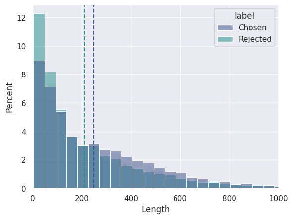
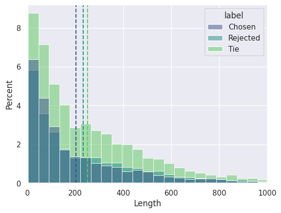
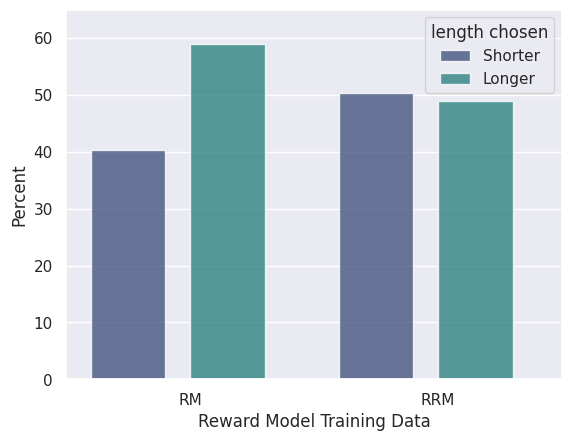
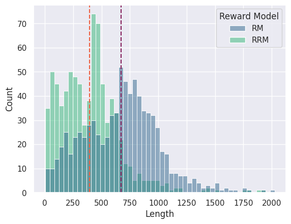
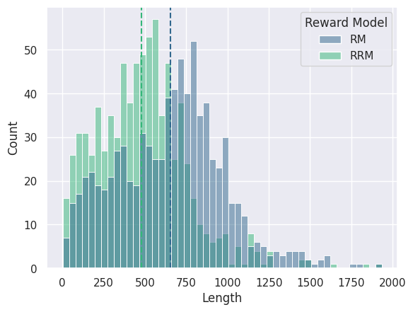
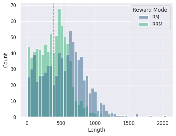
We study the length (number of tokens) distribution of reward model training datasets. Length is one common artifact that shows bias on both policy training and evaluation. We hypothesize that the bias can possibly come from the reward model training data. The one used in training RM is not well calibrated and the chosen responses are longer on average (Figure 3(a) and 3(b)) and by frequency (Figure 3(c)). On contrary, the RRM training data is better calibrated with length more balanced between chosen and rejected responses in each length bin (Figure 3(a) and 3(b)). We further provide length analysis for each data source in Appendix A.2.
Length distribution of policies
To understand the lengthy bias learned in various policies, we also study the length distribution of generated responses on AlpacaEval-2’s (Dubois et al., 2024a) prompts (Figure 4). We observe that the policies induced by RRM generate shorter responses than RM, which implies the correction of lengthy bias by RRM.
4.4 Deliberately designed artifacts
Artifacts
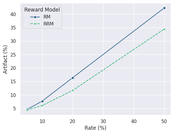
To verify that our proposed method is able to eliminate artifacts, we artificially added an artifact to the chosen responses in reward model training data. More specifically, we add prefix “Sure, here is the response: ” to the chosen responses with probability 0.1. We train an RM and RRM on the modified reward model training data, respectively.
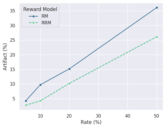
To test the effect of reward model on the policy model, we first sample responses from Gemma-2-9b-it model using the AlpacaEval-2 prompts. Then we add the same type of artifact to each response with probability , where . Under this setting, RM trained on the artifact-added data would prefer responses with the artifacts since the chosen responses come with artifacts, even if the responses may contain low-quality answer. RRM is expected to be more robust to the artifact. To verify this, we construct BoN policies using RM and RRM, respectively.
As expected, Figure 5 shows that after adding the artifacts, the BoN policies induced by RRM are more robust than RM to artifacts injected in the responses.
5 Related Works
RLHF algorithms
The first RLHF framework is based on the proximal policy optimization (PPO) algorithm, which was first popularized by Christiano et al. (2017) and further developed by Bai et al. (2022a); Ouyang et al. (2022). However, getting the deep RL method (PPO) work is challenging especially in the era of LLMs (Choshen et al., ; Engstrom et al., 2020). In recognition of this issue, another line of works proposes direct alignment algorithms, where notable examples include SLiC (Zhao et al., 2023), DPO (Rafailov et al., 2024), IPO (Azar et al., 2024), KTO (Ethayarajh et al., 2024), ORPO (Hong et al., 2024), SimPO (Meng et al., 2024), and DRO (Richemond et al., 2024). These algorithms directly optimize a supervised target to optimize the policy model without constructing a reward model first, hence the name direct alignment algorithms. However, these algorithms learning from a fixed dataset are offline and often off-policy without further exploration of the environment. RSO (Liu et al., 2024b) emphasizes the importance of reward model and fixes the distribution shift problem to improve the DPO training, followed by list-wise alignment (Liu et al., 2024a) and the online (iterative) training frameworks (Xiong et al., ; Guo et al., 2024; Calandriello et al., ). Alternatively, there is also a line of work based on the best-of-n sampling, such as RAFT (Dong et al., ), BOND (Sessa et al., 2024), BoNBoN alignment (Gui et al., 2024). These algorithms leverage a reward model to rank the generated responses and distill knowledge from the best responses. Our approach can benefit RLHF algorithms relying on a reward model.
Reward Models & Reward Hackings
Building a superhuman/unbiased reward model is vital for training better chat assistants since it could affect the upper bound of the policies’ capabilities in the online preference optimization (Wang et al., 2024a; Bai et al., 2022b). Multi-objective rewards (Wang et al., 2024b), RLHF-workflow (Dong et al., 2024), and RMBoost (Shen et al., 2024) are proposed to train more capable reward models. While revealed by Denison et al. (2024); Zhang et al. (2024), reward models are easily hacked by different pattern in different scenario, e.g., length (Singhal et al., 2023) and sycophancy. Recent works employ the model merging (WARP (Ramé et al., 2024a) and WARM (Ramé et al., 2024b)), and hacking reward decomposition (ODIN (Chen et al., )) to mitigate the hackings in online RLHF. Generative reward models can provide more detailed preference analysis (Yan et al., 2024). For the most accurate reward signal, one can also use verifiable answers in certain domain like math (Xiong et al., 2024). Most model-based methods failed to distinguish between preferences driven by the prompt and context-free artifacts. Our RRM is more advanced in removing the artifacts.
6 Conclusion
In this paper, we identified a key problem in the current reward training methodology: its inability to differentiate between contextual signals and context-free artifacts. Using a causal framework, we explained this effect and improved reward model training by introducing a data augmentation approach derived from the framework. Our theoretical analysis and extensive empirical results demonstrated that the proposed techniques effectively enhance both the test accuracy of the reward model and the quality of the policies it induces. Future work will explore filtering augmented pairs and matching artifacts when constructing response pairs, further refining the training process.
References
- Achiam et al. (2023) Josh Achiam, Steven Adler, Sandhini Agarwal, Lama Ahmad, Ilge Akkaya, Florencia Leoni Aleman, Diogo Almeida, Janko Altenschmidt, Sam Altman, Shyamal Anadkat, et al. Gpt-4 technical report. arXiv preprint arXiv:2303.08774, 2023.
- Azar et al. (2024) Mohammad Gheshlaghi Azar, Zhaohan Daniel Guo, Bilal Piot, Remi Munos, Mark Rowland, Michal Valko, and Daniele Calandriello. A general theoretical paradigm to understand learning from human preferences. In International Conference on Artificial Intelligence and Statistics, pp. 4447–4455. PMLR, 2024.
- Bai et al. (2022a) Yuntao Bai, Andy Jones, Kamal Ndousse, Amanda Askell, Anna Chen, Nova DasSarma, Dawn Drain, Stanislav Fort, Deep Ganguli, Tom Henighan, et al. Training a helpful and harmless assistant with reinforcement learning from human feedback. arXiv preprint arXiv:2204.05862, 2022a.
- Bai et al. (2022b) Yuntao Bai, Saurav Kadavath, Sandipan Kundu, Amanda Askell, Jackson Kernion, Andy Jones, Anna Chen, Anna Goldie, Azalia Mirhoseini, Cameron McKinnon, Carol Chen, Catherine Olsson, Christopher Olah, Danny Hernandez, Dawn Drain, Deep Ganguli, Dustin Li, Eli Tran-Johnson, Ethan Perez, Jamie Kerr, Jared Mueller, Jeffrey Ladish, Joshua Landau, Kamal Ndousse, Kamile Lukosuite, Liane Lovitt, Michael Sellitto, Nelson Elhage, Nicholas Schiefer, Noemi Mercado, Nova DasSarma, Robert Lasenby, Robin Larson, Sam Ringer, Scott Johnston, Shauna Kravec, Sheer El Showk, Stanislav Fort, Tamera Lanham, Timothy Telleen-Lawton, Tom Conerly, Tom Henighan, Tristan Hume, Samuel R. Bowman, Zac Hatfield-Dodds, Ben Mann, Dario Amodei, Nicholas Joseph, Sam McCandlish, Tom Brown, and Jared Kaplan. Constitutional ai: Harmlessness from ai feedback, 2022b. URL https://arxiv.org/abs/2212.08073.
- Bradley & Terry (1952) Ralph Allan Bradley and Milton E Terry. Rank analysis of incomplete block designs: I. the method of paired comparisons. Biometrika, 39(3/4):324–345, 1952.
- (6) Daniele Calandriello, Zhaohan Daniel Guo, Remi Munos, Mark Rowland, Yunhao Tang, Bernardo Avila Pires, Pierre Harvey Richemond, Charline Le Lan, Michal Valko, Tianqi Liu, et al. Human alignment of large language models through online preference optimisation. In Forty-first International Conference on Machine Learning.
- (7) Lichang Chen, Chen Zhu, Jiuhai Chen, Davit Soselia, Tianyi Zhou, Tom Goldstein, Heng Huang, Mohammad Shoeybi, and Bryan Catanzaro. Odin: Disentangled reward mitigates hacking in rlhf. In Forty-first International Conference on Machine Learning.
- (8) Leshem Choshen, Lior Fox, Zohar Aizenbud, and Omri Abend. On the weaknesses of reinforcement learning for neural machine translation. In International Conference on Learning Representations.
- Christiano et al. (2017) Paul F Christiano, Jan Leike, Tom Brown, Miljan Martic, Shane Legg, and Dario Amodei. Deep reinforcement learning from human preferences. Advances in neural information processing systems, 30, 2017.
- Cui et al. (2023) Ganqu Cui, Lifan Yuan, Ning Ding, Guanming Yao, Wei Zhu, Yuan Ni, Guotong Xie, Zhiyuan Liu, and Maosong Sun. Ultrafeedback: Boosting language models with high-quality feedback, 2023.
- Daniele & Suphavadeeprasit (2023) Luigi Daniele and Suphavadeeprasit. Amplify-instruct: Synthetically generated diverse multi-turn conversations for effecient llm training. arXiv preprint arXiv:(coming soon), 2023. URL https://huggingface.co/datasets/LDJnr/Capybara.
- Denison et al. (2024) Carson Denison, Monte MacDiarmid, Fazl Barez, David Duvenaud, Shauna Kravec, Samuel Marks, Nicholas Schiefer, Ryan Soklaski, Alex Tamkin, Jared Kaplan, Buck Shlegeris, Samuel R. Bowman, Ethan Perez, and Evan Hubinger. Sycophancy to subterfuge: Investigating reward-tampering in large language models, 2024. URL https://arxiv.org/abs/2406.10162.
- (13) Hanze Dong, Wei Xiong, Deepanshu Goyal, Yihan Zhang, Winnie Chow, Rui Pan, Shizhe Diao, Jipeng Zhang, SHUM KaShun, and Tong Zhang. Raft: Reward ranked finetuning for generative foundation model alignment. Transactions on Machine Learning Research.
- Dong et al. (2024) Hanze Dong, Wei Xiong, Bo Pang, Haoxiang Wang, Han Zhao, Yingbo Zhou, Nan Jiang, Doyen Sahoo, Caiming Xiong, and Tong Zhang. Rlhf workflow: From reward modeling to online rlhf. arXiv preprint arXiv:2405.07863, 2024.
- Dubois et al. (2024a) Yann Dubois, Balázs Galambosi, Percy Liang, and Tatsunori B Hashimoto. Length-controlled alpacaeval: A simple way to debias automatic evaluators. arXiv preprint arXiv:2404.04475, 2024a.
- Dubois et al. (2024b) Yann Dubois, Chen Xuechen Li, Rohan Taori, Tianyi Zhang, Ishaan Gulrajani, Jimmy Ba, Carlos Guestrin, Percy S Liang, and Tatsunori B Hashimoto. Alpacafarm: A simulation framework for methods that learn from human feedback. Advances in Neural Information Processing Systems, 36, 2024b.
- Eisenstein et al. (2023) Jacob Eisenstein, Chirag Nagpal, Alekh Agarwal, Ahmad Beirami, Alex D’Amour, DJ Dvijotham, Adam Fisch, Katherine Heller, Stephen Pfohl, Deepak Ramachandran, et al. Helping or herding? reward model ensembles mitigate but do not eliminate reward hacking. arXiv preprint arXiv:2312.09244, 2023.
- Engstrom et al. (2020) Logan Engstrom, Andrew Ilyas, Shibani Santurkar, Dimitris Tsipras, Firdaus Janoos, Larry Rudolph, and Aleksander Madry. Implementation matters in deep policy gradients: A case study on ppo and trpo. arXiv preprint arXiv:2005.12729, 2020.
- Ethayarajh et al. (2022) Kawin Ethayarajh, Yejin Choi, and Swabha Swayamdipta. Understanding dataset difficulty with v-usable information. In International Conference on Machine Learning, pp. 5988–6008. PMLR, 2022.
- Ethayarajh et al. (2024) Kawin Ethayarajh, Winnie Xu, Niklas Muennighoff, Dan Jurafsky, and Douwe Kiela. Kto: Model alignment as prospect theoretic optimization. arXiv preprint arXiv:2402.01306, 2024.
- Gao et al. (2023) Leo Gao, John Schulman, and Jacob Hilton. Scaling laws for reward model overoptimization. In International Conference on Machine Learning, pp. 10835–10866. PMLR, 2023.
- Gui et al. (2024) Lin Gui, Cristina Gârbacea, and Victor Veitch. Bonbon alignment for large language models and the sweetness of best-of-n sampling. arXiv preprint arXiv:2406.00832, 2024.
- Guo et al. (2024) Shangmin Guo, Biao Zhang, Tianlin Liu, Tianqi Liu, Misha Khalman, Felipe Llinares, Alexandre Rame, Thomas Mesnard, Yao Zhao, Bilal Piot, et al. Direct language model alignment from online ai feedback. arXiv preprint arXiv:2402.04792, 2024.
- Hong et al. (2024) Jiwoo Hong, Noah Lee, and James Thorne. Reference-free monolithic preference optimization with odds ratio. arXiv preprint arXiv:2403.07691, 2024.
- Ji et al. (2024) Jiaming Ji, Mickel Liu, Josef Dai, Xuehai Pan, Chi Zhang, Ce Bian, Boyuan Chen, Ruiyang Sun, Yizhou Wang, and Yaodong Yang. Beavertails: Towards improved safety alignment of llm via a human-preference dataset. Advances in Neural Information Processing Systems, 36, 2024.
- Jiang et al. (2023) Dongfu Jiang, Xiang Ren, and Bill Yuchen Lin. Llm-blender: Ensembling large language models with pairwise ranking and generative fusion. arXiv preprint arXiv:2306.02561, 2023.
- Lambert et al. (2024) Nathan Lambert, Valentina Pyatkin, Jacob Morrison, LJ Miranda, Bill Yuchen Lin, Khyathi Chandu, Nouha Dziri, Sachin Kumar, Tom Zick, Yejin Choi, et al. Rewardbench: Evaluating reward models for language modeling. arXiv preprint arXiv:2403.13787, 2024.
- Lauritzen (1996) Steffen L Lauritzen. Graphical models, volume 17. Clarendon Press, 1996.
- Lee et al. (2020) Kuang-Yao Lee, Tianqi Liu, Bing Li, and Hongyu Zhao. Learning causal networks via additive faithfulness. Journal of Machine Learning Research, 21(51):1–38, 2020.
- Lehmann & Casella (2006) Erich L Lehmann and George Casella. Theory of point estimation. Springer Science & Business Media, 2006.
- Lian et al. (2023) Wing Lian, Bleys Goodson, Eugene Pentland, Austin Cook, Chanvichet Vong, and ”Teknium”. Openorca: An open dataset of gpt augmented flan reasoning traces. https://https://huggingface.co/Open-Orca/OpenOrca, 2023.
- Lin et al. (2023) Yong Lin, Lu Tan, Hangyu Lin, Zeming Zheng, Renjie Pi, Jipeng Zhang, Shizhe Diao, Haoxiang Wang, Han Zhao, Yuan Yao, et al. Speciality vs generality: An empirical study on catastrophic forgetting in fine-tuning foundation models. arXiv preprint arXiv:2309.06256, 2023.
- Liu et al. (2024a) Tianqi Liu, Zhen Qin, Junru Wu, Jiaming Shen, Misha Khalman, Rishabh Joshi, Yao Zhao, Mohammad Saleh, Simon Baumgartner, Jialu Liu, Peter J. Liu, and Xuanhui Wang. Lipo: Listwise preference optimization through learning-to-rank, 2024a. URL https://arxiv.org/abs/2402.01878.
- Liu et al. (2024b) Tianqi Liu, Yao Zhao, Rishabh Joshi, Misha Khalman, Mohammad Saleh, Peter J Liu, and Jialu Liu. Statistical rejection sampling improves preference optimization. In The Twelfth International Conference on Learning Representations, 2024b.
- Loshchilov (2017) I Loshchilov. Decoupled weight decay regularization. arXiv preprint arXiv:1711.05101, 2017.
- Meng et al. (2024) Yu Meng, Mengzhou Xia, and Danqi Chen. Simpo: Simple preference optimization with a reference-free reward. arXiv preprint arXiv:2405.14734, 2024.
- Ouyang et al. (2022) Long Ouyang, Jeffrey Wu, Xu Jiang, Diogo Almeida, Carroll Wainwright, Pamela Mishkin, Chong Zhang, Sandhini Agarwal, Katarina Slama, Alex Ray, et al. Training language models to follow instructions with human feedback. Advances in neural information processing systems, 35:27730–27744, 2022.
- Pace et al. (2024) Alizée Pace, Jonathan Mallinson, Eric Malmi, Sebastian Krause, and Aliaksei Severyn. West-of-n: Synthetic preference generation for improved reward modeling. arXiv preprint arXiv:2401.12086, 2024.
- Park et al. (2024) Ryan Park, Rafael Rafailov, Stefano Ermon, and Chelsea Finn. Disentangling length from quality in direct preference optimization. arXiv preprint arXiv:2403.19159, 2024.
- Pearl (2009) Judea Pearl. Causality. Cambridge university press, 2009.
- Rafailov et al. (2024) Rafael Rafailov, Archit Sharma, Eric Mitchell, Christopher D Manning, Stefano Ermon, and Chelsea Finn. Direct preference optimization: Your language model is secretly a reward model. Advances in Neural Information Processing Systems, 36, 2024.
- Ramé et al. (2024a) Alexandre Ramé, Johan Ferret, Nino Vieillard, Robert Dadashi, Léonard Hussenot, Pierre-Louis Cedoz, Pier Giuseppe Sessa, Sertan Girgin, Arthur Douillard, and Olivier Bachem. Warp: On the benefits of weight averaged rewarded policies, 2024a. URL https://arxiv.org/abs/2406.16768.
- Ramé et al. (2024b) Alexandre Ramé, Nino Vieillard, Léonard Hussenot, Robert Dadashi, Geoffrey Cideron, Olivier Bachem, and Johan Ferret. Warm: On the benefits of weight averaged reward models, 2024b. URL https://arxiv.org/abs/2401.12187.
- Richemond et al. (2024) Pierre Harvey Richemond, Yunhao Tang, Daniel Guo, Daniele Calandriello, Mohammad Gheshlaghi Azar, Rafael Rafailov, Bernardo Avila Pires, Eugene Tarassov, Lucas Spangher, Will Ellsworth, et al. Offline regularised reinforcement learning for large language models alignment. arXiv preprint arXiv:2405.19107, 2024.
- Schulman et al. (2017) John Schulman, Filip Wolski, Prafulla Dhariwal, Alec Radford, and Oleg Klimov. Proximal policy optimization algorithms. arXiv preprint arXiv:1707.06347, 2017.
- Sessa et al. (2024) Pier Giuseppe Sessa, Robert Dadashi, Léonard Hussenot, Johan Ferret, Nino Vieillard, Alexandre Ramé, Bobak Shariari, Sarah Perrin, Abe Friesen, Geoffrey Cideron, et al. Bond: Aligning llms with best-of-n distillation. arXiv preprint arXiv:2407.14622, 2024.
- Shen et al. (2024) Jiaming Shen, Ran Xu, Yennie Jun, Zhen Qin, Tianqi Liu, Carl Yang, Yi Liang, Simon Baumgartner, and Michael Bendersky. Boosting reward model with preference-conditional multi-aspect synthetic data generation. arXiv preprint arXiv:2407.16008, 2024.
- Shen et al. (2023a) Lingfeng Shen, Sihao Chen, Linfeng Song, Lifeng Jin, Baolin Peng, Haitao Mi, Daniel Khashabi, and Dong Yu. The trickle-down impact of reward (in-) consistency on rlhf. arXiv preprint arXiv:2309.16155, 2023a.
- Shen et al. (2023b) Wei Shen, Rui Zheng, Wenyu Zhan, Jun Zhao, Shihan Dou, Tao Gui, Qi Zhang, and Xuanjing Huang. Loose lips sink ships: Mitigating length bias in reinforcement learning from human feedback. arXiv preprint arXiv:2310.05199, 2023b.
- Singhal et al. (2023) Prasann Singhal, Tanya Goyal, Jiacheng Xu, and Greg Durrett. A long way to go: Investigating length correlations in rlhf. arXiv preprint arXiv:2310.03716, 2023.
- Team et al. (2023) Gemini Team, Rohan Anil, Sebastian Borgeaud, Yonghui Wu, Jean-Baptiste Alayrac, Jiahui Yu, Radu Soricut, Johan Schalkwyk, Andrew M Dai, Anja Hauth, et al. Gemini: a family of highly capable multimodal models. arXiv preprint arXiv:2312.11805, 2023.
- VanderWeele (2011) Tyler J VanderWeele. Controlled direct and mediated effects: definition, identification and bounds. Scandinavian Journal of Statistics, 38(3):551–563, 2011.
- Wang et al. (2024a) Binghai Wang, Rui Zheng, Lu Chen, Yan Liu, Shihan Dou, Caishuang Huang, Wei Shen, Senjie Jin, Enyu Zhou, Chenyu Shi, Songyang Gao, Nuo Xu, Yuhao Zhou, Xiaoran Fan, Zhiheng Xi, Jun Zhao, Xiao Wang, Tao Ji, Hang Yan, Lixing Shen, Zhan Chen, Tao Gui, Qi Zhang, Xipeng Qiu, Xuanjing Huang, Zuxuan Wu, and Yu-Gang Jiang. Secrets of rlhf in large language models part ii: Reward modeling, 2024a. URL https://arxiv.org/abs/2401.06080.
- Wang et al. (2024b) Haoxiang Wang, Wei Xiong, Tengyang Xie, Han Zhao, and Tong Zhang. Interpretable preferences via multi-objective reward modeling and mixture-of-experts, 2024b. URL https://arxiv.org/abs/2406.12845.
- Wang et al. (2023) Zhilin Wang, Yi Dong, Jiaqi Zeng, Virginia Adams, Makesh Narsimhan Sreedhar, Daniel Egert, Olivier Delalleau, Jane Polak Scowcroft, Neel Kant, Aidan Swope, and Oleksii Kuchaiev. Helpsteer: Multi-attribute helpfulness dataset for steerlm, 2023.
- (56) Wei Xiong, Hanze Dong, Chenlu Ye, Ziqi Wang, Han Zhong, Heng Ji, Nan Jiang, and Tong Zhang. Iterative preference learning from human feedback: Bridging theory and practice for rlhf under kl-constraint. In Forty-first International Conference on Machine Learning.
- Xiong et al. (2024) Wei Xiong, Chengshuai Shi, Jiaming Shen, Aviv Rosenberg, Zhen Qin, Daniele Calandriello, Misha Khalman, Rishabh Joshi, Bilal Piot, Mohammad Saleh, et al. Building math agents with multi-turn iterative preference learning. arXiv preprint arXiv:2409.02392, 2024.
- Yan et al. (2024) Jing Nathan Yan, Tianqi Liu, Justin Chiu, Jiaming Shen, Zhen Qin, Yue Yu, Charumathi Lakshmanan, Yair Kurzion, Alexander Rush, Jialu Liu, and Michael Bendersky. Predicting text preference via structured comparative reasoning. In Lun-Wei Ku, Andre Martins, and Vivek Srikumar (eds.), Proceedings of the 62nd Annual Meeting of the Association for Computational Linguistics (Volume 1: Long Papers), pp. 10040–10060, Bangkok, Thailand, August 2024. Association for Computational Linguistics. URL https://aclanthology.org/2024.acl-long.541.
- Ye et al. (2024) Chenlu Ye, Wei Xiong, Yuheng Zhang, Nan Jiang, and Tong Zhang. A theoretical analysis of nash learning from human feedback under general kl-regularized preference. arXiv preprint arXiv:2402.07314, 2024.
- Yuan et al. (2024) Lifan Yuan, Ganqu Cui, Hanbin Wang, Ning Ding, Xingyao Wang, Jia Deng, Boji Shan, Huimin Chen, Ruobing Xie, Yankai Lin, Zhenghao Liu, Bowen Zhou, Hao Peng, Zhiyuan Liu, and Maosong Sun. Advancing llm reasoning generalists with preference trees, 2024.
- Zhang et al. (2024) Xuanchang Zhang, Wei Xiong, Lichang Chen, Tianyi Zhou, Heng Huang, and Tong Zhang. From lists to emojis: How format bias affects model alignment, 2024. URL https://arxiv.org/abs/2409.11704.
- Zhao et al. (2023) Yao Zhao, Rishabh Joshi, Tianqi Liu, Misha Khalman, Mohammad Saleh, and Peter J Liu. Slic-hf: Sequence likelihood calibration with human feedback. arXiv preprint arXiv:2305.10425, 2023.
- Zhao et al. (2021) Zihao Zhao, Eric Wallace, Shi Feng, Dan Klein, and Sameer Singh. Calibrate before use: Improving few-shot performance of language models. In International conference on machine learning, pp. 12697–12706. PMLR, 2021.
- Zheng et al. (2024) Lianmin Zheng, Wei-Lin Chiang, Ying Sheng, Siyuan Zhuang, Zhanghao Wu, Yonghao Zhuang, Zi Lin, Zhuohan Li, Dacheng Li, Eric Xing, et al. Judging llm-as-a-judge with mt-bench and chatbot arena. Advances in Neural Information Processing Systems, 36, 2024.
- Ziegler et al. (2019) Daniel M Ziegler, Nisan Stiennon, Jeffrey Wu, Tom B Brown, Alec Radford, Dario Amodei, Paul Christiano, and Geoffrey Irving. Fine-tuning language models from human preferences. arXiv preprint arXiv:1909.08593, 2019.
Appendix A Appendix
A.1 Proofs
Proof of Proposition 3.1
Proof.
We show the conclusion with a special case. Assume with , and with . with constants and random error . If , then is true. If , then is true. In extreme case that , then for some constants and . Then the model cannot tell if or not. This is because when , we can still reparametrize it as . ∎
Proof of Proposition 3.2
Proof.
We can prove this by contradiction. If there is a causal edge from to , then the conditional independence relations and do not hold, which contracts to the triplets constructed on “Non-contextuals” and “Neutrals”. ∎
A.2 Reward Model Training Datasets
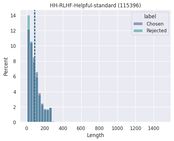
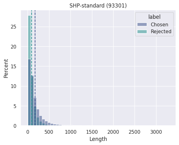
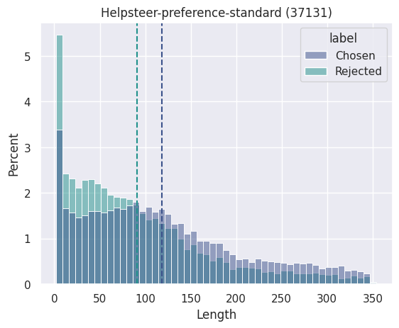
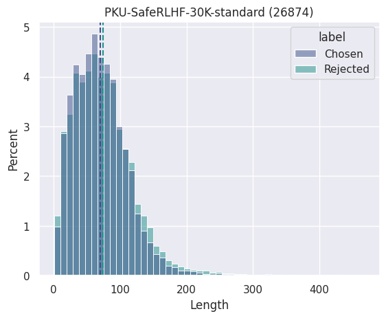
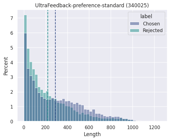
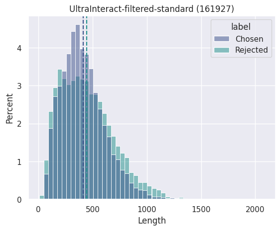
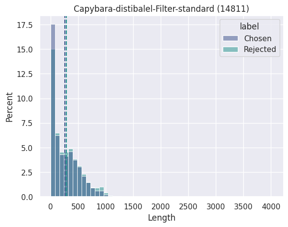
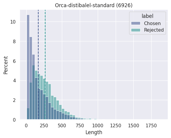
We reuse the datasets in RLHFlow (Dong et al., 2024). We list the data sources and number of examples in Table 3. The authors of the original paper delete the samples with similar scores when the scores are available because when the model is well calibrated, these samples are more likely to mislabelled. Thus the total number is smaller than the sum of each individual datasets. We show the length distribution of chosen and rejected responses from each individual data source in Figure 6. HH-RLHF, SHP, HelpSteer, UltraFeedback show bias towards rejected responses as the first length bin. SHP, HelpSteer, and UltraFeedback have longer chosen responses than rejected ones on average.
| Source | Number of Examples |
|---|---|
| HH-RLHF-Helpful888https://huggingface.co/datasets/RLHFlow/HH-RLHF-Helpful-standard (Bai et al., 2022a) | 115,396 |
| SHP999https://huggingface.co/datasets/RLHFlow/SHP-standard (Ethayarajh et al., 2022) | 93,301 |
| HelpSteer101010https://huggingface.co/datasets/RLHFlow/Helpsteer-preference-standard(Wang et al., 2023) | 37,131 |
| PKU-SafeRLHF111111https://huggingface.co/datasets/RLHFlow/PKU-SafeRLHF-30K-standard (Ji et al., 2024) | 26,874 |
| UltraFeedback121212https://huggingface.co/datasets/RLHFlow/UltraFeedback-preference-standard (Cui et al., 2023) | 340,025 |
| UltraInteract131313https://huggingface.co/datasets/RLHFlow/UltraInteract-filtered-standard (Yuan et al., 2024) | 161,927 |
| Distilabel-Capybara141414https://huggingface.co/datasets/RLHFlow/Capybara-distibalel-Filter-standard (Daniele & Suphavadeeprasit, 2023) | 14,811 |
| Distilabel-Orca151515https://huggingface.co/datasets/RLHFlow/Orca-distibalel-standard (Lian et al., 2023) | 6,926 |
A.3 Data augmentation python code
In Algorithm 1, we show a sample code of data augmentation in Python. We expect each element in data contains “context”, “response_w”, “response_l”. We use “neutral” to indicate if the label should be “tie”.
A.4 Training details for ODIN
We use the same loss as described in Chen et al. . We train Gemma-2-9b-it for 1 epoch on the same data we used for RM. AdamW is our optimizer and the learning rate is set to 2e-6 with cosine scheduler. We use Flash-Attention to accelerate the training while applying the Deepspeed Zero-Stage 3 to get batch_size=16 on each GPU (the global batch size is 128) to make sure the calculation of the Pearson correlation between the head value and the length of the responses is stable.
A.5 Preliminaries in Causal inference
We list a few critical concepts in this section. For information, we refer the readers to Lauritzen (1996) and Pearl (2009).
DAGs and d-separation
A DAG is a set of vertices and a set of directed edges (arrows) that connect pairs of these vertices. The causal modeling connects a DAG with Markov condition via a graphical relation called d-separation (Pearl, 2009). D-separation is a relation among three disjoint sets of vertices in a directed graph. D-separation and Markov condition connect DAGs and probability distribution. By faithfulness assumption, the d-separation in a DAG is equivalent to conditional independence in distribution.
The Causal Markov Condition
The Causal Markov assumption assumes that a variable is independent of every other variable (except ’s effects) conditional on all of its direct causes. With this, a DAG defines a set of distributions of the form
Counterfactuals
Consider two variables and . We will call the “treatment”. We call the “outcome”. For a given subject we see . What we don’t see is what their value of would have been if we changed their value of . This is called counterfactual. Suppose that is a binary variable that represents some treatment. So means the subject was treated and means the subject was not treated. Let denote the outcome if the subject is treated. Let denote the response if the subject is not treated. Then
If we treat a subject, we observe but not . The unobserved variable is called a counterfactual. The variables are also called potential outcomes. We define mean treatment effect as