Joint Graph Rewiring and Feature Denoising via Spectral Resonance

Abstract

Graph neural networks (GNNs) take as input the graph structure and the feature vectors associated with the nodes. Both contain noisy information about the labels. Here we propose joint denoising and rewiring (JDR)—an algorithm to jointly denoise the graph structure and features, which can improve the performance of any downstream GNN. We do this by defining and maximizing the alignment between the leading eigenspaces of graph and feature matrices. To approximately solve this computationally hard problem, we propose a heuristic that efficiently handles real-world graph datasets with many classes and different levels of homophily or heterophily. We experimentally verify the effectiveness of our approach on synthetic data and real-world graph datasets. The results show that JDR consistently outperforms existing rewiring methods on node classification tasks using GNNs as downstream models.

1 Introduction

Graph neural networks (GNNs) are a powerful deep learning tool for graph-structured data, with applications in physics [26, 22], chemistry [17], biology [18] and beyond [41]. Typical tasks across disciplines include graph classification [20, 5], node classification [21, 8] and link prediction [31].

Graph data contains two distinct types of information, the graph structure and the node features. The graph encodes interactions between entities and thus the classes or communities they belong to, similarly to the features. Since real-world graphs and features contain noise, we ask a natural question: Is there a simple way to jointly denoise the graph and the features which improves performance of any downstream GNN?

Indeed, recent work demonstrates that rewiring the graph by judiciously adding and removing edges may improve GNN performance by facilitating information flow. In a GNN, the graph serves not only to encode interactions but also to organize computations [17, 4]. So even when it correctly encodes interactions it may not be an effective computational graph due to conditions such as oversquashing [2] and oversmoothing [6]. Existing rewiring methods use geometric and spectral properties of the graph, including curvature [38, 30, 14], expansion [9, 3], effective resistance [5], and spectral gap [19]. They are feature-agnostic, which makes them suitable for graphs both with and without node features.

Figure 1: Schematic overview of joint denoising and rewiring (JDR). In this example, we consider a noisy graph in the sense that it contains edges between and within classes and its node features are not fully aligned with the labels. This is useful, because it models different practical scenarios of real-world graphs. The graph is represented by its adjacency matrix $\bm{A}$ and binary node features $\bm{X}$, both of which can be decomposed via spectral decomposition and SVD. The denoising of $\bm{X}$ is performed by combining the information of its own eigenvectors $\bm{U}$ and the eigenvectors $\bm{V}$ from $\bm{A}$. The same applies vice versa for rewiring, and both are performed iteratively $K$ times. The rewired graph $\tilde{\bm{A}}$ and the denoised features $\tilde{\bm{X}}$ result from graph synthesis by multiplying back with the final $\bm{V}_{(K)}$ and $\bm{U}_{(K)}$. To get specific properties like sparsity or binarity we can perform an Update step, e.g. by thresholding (as done here). The resulting denoised and rewired graph is displayed on the right. By adding four edges and removing three, its structure now almost perfectly represents the communities. The features have also been improved, as the first entry now indicates the class assignment.

In many real graphs, however, the features contain valuable information about the node labels. This fact is implicit in high-quality stylized models of graphs with features, including community models such as the contextual stochastic block model (cSBM) [10, 35] and neighborhood graphs on points from low-dimensional manifolds. In the latter case features are often related to low-dimensional coordinates, motivating various spectral clustering and non-linear dimensionality reduction methods [36, 29]. In cSBM, seminal theoretical work shows that jointly leveraging the graph (SBM) and the features (a GMM) improves over unsupervised clustering using either piece of information alone. The quantities used to characterize recovery bounds in [10] (which we mention below) are computationally hard. While there exist efficient algorithms based on belief propagation [10] (also for the semi-supervised setting [12]), they are essentially based on the perfect knowledge of the distribution of the cSBM.

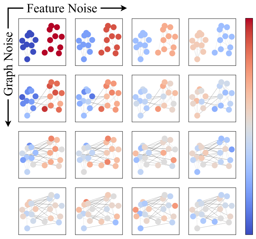
In this paper: (1) We take inspiration from the work on cSBM to design a practical algorithm for joint graph rewiring and feature denoising, which can improve the node classification performance of any downstream GNN on arbitrary real-world datasets. We achieve this denoising by perturbing the graph and the features so as to maximize alignment between their leading eigenspaces. If these spaces are well-aligned we say that the graph and the features are in resonance. (2) Our major contribution is an alternating optimization algorithm, joint denoising and rewiring (JDR), to approximately solve the computationally hard alignment maximization problem for real-world graph data which contains multiple classes and may be homophilic or heterophilic and thus spectrally complex. Our method is outlined in Figure 1 and the code repository is available online. (3) We show that JDR outperforms existing geometric rewiring strategies while being guided only by denoising. This suggests that although there exist (or we can design) graphs with topological and geometrical characteristics which make existing rewiring schemes beneficial, a greater issue in real-world graphs is noise in the sense of missing and spurious links. This is true even when graphs correctly reflect the ground truth information. In a citation network, for example, citations that should exist may be missing because of incomplete scholarship. Conversely, citations that should not exist may be present because the authors engaged in bibliographic ornamentation.

Organization of the Paper. After discussing the relation to prior work in Section 2, we introduce JDR in Section 3; we motivate it by insights from the cSBM [10]. In Section 4 we present the experimental results of our method on synthetic and real-world data, showing that it consistently outperforms current rewiring methods. Section 5 concludes by discussing the main findings, listing limitations and providing suggestions for future research.

2 Relation to Prior Work

There is an extensive literature on denoising signals on graphs using graph filters [25, 23]. However, we are interested in denoising the structure of the graph itself, in a way that can benefit any downstream algorithm. Another related line of work is on graph structure learning [43]. Several works address noise in graphs and node features [7, 39, 44] with the aim to make GNNs more robust against adversarial perturbations or to learn a graph for data when there is no graph to start with. Our aim is different: to improve the overall node classification performance of GNNs. Lv et al. [24] build a neighborhood graph over features and interpolate between it and the input graph, which is a form of alignment. They however do not use spectral information and do not deal with noise in the features. Further, their method is only suitable for homophilic graphs where similarity-based connection rules apply. Some of these methods also have difficulties when applied to very low-noise graphs [11], while our method can naturally deal with this by adapting to the signal-to-noise ratio (SNR) of the graph and the features.

Conceptually-related work uses diffusion-based rewiring [16] that smooths out the graph adjacency. This can be interpreted as graph denoising, but is again only suitable for homophilic graphs. Our approach is related to rewiring but with several key differences. We modify the graph purely from a denoising perspective, while the classical rewiring literature [38, 30, 14] relies on geometric notions, focusing on optimizing the graph for message passing computations. While there exist rewiring works that leverage the graph spectrum [19], a major difference is that we denoise both the graph and the node features, in a way that adapts to the quality of either source of information.

3 Joint Denoising and Rewiring

3.1 Preliminaries

We let $\mathcal{G}=(\mathcal{V},\mathcal{E})$ be an undirected graph with $|\mathcal{V}|=N$ nodes and an adjacency matrix $\bm{A}$. To each node we associate an $F$-dimensional feature vector and collect these vectors in the rows of matrix $\bm{X}\in\mathbb{R}^{N\times F}$. We make extensive use of the graph and feature spectra, namely the eigendecomposition $\bm{A}=\bm{V}\bm{\Lambda}\bm{V}^{T}$ and the SVD $\bm{X}=\bm{U}\bm{\Sigma}\bm{W}^{T}$, with eigen- and singular values ordered from largest to smallest. (As discussed below, in heterophilic graphs we order the eigenvalues of $\bm{A}$ according to their absolute value.) The graph Laplacian is $\bm{L}=\bm{D}-\bm{A}$, where $\bm{D}$ is the diagonal node degree matrix. For $k>2$ node classes, we use one-hot labels $\bm{y}\in\{0,1\}^{N\times k}$. We write $[L]$ for the set $\{1,2,\ldots,L\}$. In the balanced two-class case, we consider nodes to be ordered so that the first half has label $\bm{y}_{i}=-1$ and the second half $\bm{y}_{i}=1$. In semi-supervised node classification, which we are interested in, the task is to label the nodes based on the graph ($\bm{A}$ and $\bm{X}$) and a subset of the labels $\bm{y}$. Homophilic graphs are those where nodes are more likely to connect with nodes with similar features or labels (e.g., friendship networks [28]); heterophilic graphs are those where nodes more likely to connect with dissimilar nodes (e.g., protein interaction networks [42]).

3.2 Motivation via the contextual stochastic block model

For simplicity, we first explain our method for $k=2$ classes and graphs generated from the contextual stochastic block model (cSBM)[10]. We then extend it to real-world graphs with multiple classes and describe the full practical algorithm.

Contextual Stochastic Block Model. The cSBM extends the stochastic block model (SBM) [1], a community graph model, by high-dimensional node features [10]. In a balanced 2-class SBM the nodes are divided into two equal-sized communities with node labels $\bm{y}_{i}\in\left\{\pm 1\right\}$. Pairs of nodes connect independently at random. The probability that a node is connected to a node of its own community (intra-class) is $c_{\text{in}}/N$; the probability that it is connected to a node from the other community (inter-class) is $c_{\text{out}}/N$.

In the sparse regime [1], when the average node degree is $d=\mathcal{O}(1)$, it is common to parameterize $c_{\text{in}}=d+\lambda\sqrt{d}$ and $c_{\text{out}}=d-\lambda\sqrt{d}$. Here, $|\lambda|$ can be seen as the SNR of the graph. The signal $\bm{X}_{i}\in\mathbb{R}^{F}$ at node $i$ follows a Gaussian mixture model (GMM)

$$\bm{X}_{i}=\sqrt{\frac{\mu}{N}}\bm{y}_{i}\bm{u}+\frac{\bm{z}_{i}}{\sqrt{F}},$$ (1)

where $\bm{u}\sim\mathcal{N}\left(0,\bm{I}_{F}/F\right)$ is the randomly drawn mean and $\bm{z}_{i}\sim\mathcal{N}\left(0,\bm{I}_{F}\right)$ is i.i.d. Gaussian standard noise. We set $\frac{N}{F}=\gamma$ and following prior works [8], we parameterize the graphs generated from the cSBM using $\phi=\frac{2}{\pi}\arctan(\lambda\sqrt{\gamma}/\mu)$. For $\phi\to 1$ we get homophilic behavior; for $\phi\to-1$ we get heterophilic behavior. Close to either extreme the node features contain little information. For $\phi\to 0$ the graph is Erdős–Rényi and only the features contain information.

Denoising the cSBM. In the cSBM, $\bm{A}$ and $\bm{X}$ offer different noisy views of label information. One can show that up to a scaling and a shift, the adjacency matrix is approximately $\pm\bm{y}\bm{y}^{T}+\bm{Z}_{ER},$ which means that up to a scaling and a shift, it is approximately a rank-one matrix with labels in the range, corrupted with “Erdős–Rényi-like noise” $\bm{Z}_{ER}$ [13]. It similarly follows directly from the definition that the feature matrix $\bm{X}$ is approximately (again up to a scaling and a shift) $\bm{y}\bm{u}^{T}+\bm{Z}_{G}$ where $\bm{Z}_{G}$ is white Gaussian noise. It thus makes sense to use the information from $\bm{X}$ to enhance $\bm{A}$ and vice versa. It is shown in [10] that the right way to do this for unsupervised community detection for $k=2$ is by solving

$$\operatorname*{maximize}_{\bm{v}\in\mathbb{R}^{N},\bm{u}\in\mathbb{R}^{F}}\leavevmode\nobreak\ \langle\bm{v},\bm{Av}\rangle+b\langle\bm{v},\bm{Xu}\rangle$$ (2)

$$\mathrm{subject\leavevmode\nobreak\ to}\leavevmode\nobreak\ \|\bm{v}\|_{2}=\|\bm{u}\|_{2}=1,\langle\bm{v},\textbf{1}\rangle\approx 0.$$

for a carefully chosen value of $b$. The $\langle\bm{v},\textbf{1}\rangle\approx 0$ constraint ensures that we do not get the near-constant leading eigenvector of $\bm{A}$.

It is easy to see that in the high-SNR case, when the second leading eigenvector of $\bm{A}$ and the leading left singular vectors $\bm{X}$ approximately coincide with the labels, the optimal $\bm{v}^{*}$ is related to those singular vectors and aligned with the labels. Deshpande et al. [10] show that this formulation is optimal under some additional assumptions even in the low-SNR case. This suggests the following rationale for denoising:

• We can interpret the value of (2) as a measure of alignment. Since $\bm{v}^{*}$ corresponds to the labels, we can relate this measure to the quality of the label estimation.

• We may leverage this alignment to denoise the graph. Namely, we could perturb $\bm{A}$ and $\bm{X}$ in a way that improves the alignment.

In real datasets, however, the optimal value of $b$ is unknown, the scaling of $\bm{X}$ is arbitrary, and multiple classes complicate things. Moreover, (2) is computationally hard. We thus define a simple related measure of alignment which alleviates these issues.

Definition 1.

Recall the spectral decompositions $\bm{A}=\bm{V\Lambda V}^{T}$, $\bm{X}=\bm{U\Sigma W}^{T}$, and let $\bm{V}_{L}$, $\bm{U}_{L}$ denote the first $L$ columns of $\bm{V}$ and $\bm{U}$. We define the graph–feature alignment as

$$\mathrm{Alignment}_{L}(\bm{A},\bm{X})=\|\bm{V}_{L}^{T}\bm{U}_{L}\|_{\mathrm{sp}}.$$ (3)

Remark: The logic of this definition is that for a cSBM with high SNR and $k$ classes, the information about labels is indeed contained in the leading $L=k$ vectors of $\bm{V}$ and $\bm{U}$. The quantity $\mathrm{Alignment}_{L}(\bm{A},\bm{X})$ is the cosine of the angle between the subspaces spanned by the columns of $\bm{V}_{L}$ and $\bm{U}_{L}$. To denoise the features and rewire the graph, we seek to maximize the alignment.

Definition 2.

Given $\mathrm{Alignment}_{L}(\bm{A},\bm{X})$ and a graph with $\bm{A}_{0}$ and $\bm{X}_{0}$, we define the jointly denoised graph and features as a solution to

$$\operatorname*{maximize}_{\bm{A},\bm{X}}\mathrm{Alignment}_{L}(\bm{A},\bm{X})$$ (4)

$$\mathrm{subject\leavevmode\nobreak\ to}\leavevmode\nobreak\ \bm{A}\approx\bm{A}_{0},\bm{X}\approx\bm{X}_{0}.$$

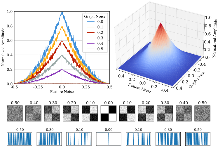
The meaning of $\approx$ may be, for instance, proximity in some matrix norm. We do not make it specific here, but mention that it is implicit in the design of our algorithm. We will show empirically that a stronger alignment indicates a better representation of the labels by $\bm{A}$ and $\bm{X}$ and thus a better graph. Figure 2 visualizes this connection between eigenvector alignment and denoising. It shows that the response of the graph to features is maximized when the spectra of the graph and the features are aligned. We refer to the condition where the alignment is high as spectral resonance; for further discussion see Section 3.3.

(a)

(b)

Figure 2: An illustration of spectral alignment and resonance. In (2(a)) we plot $\bm{\hat{x}}=\bm{x}^{T}\bm{A}\bm{x}$ for different noise levels in $\bm{A}$ and $\bm{x}\in\{-1,1\}^{N}$, illustrated in the rows below. Without noise, $\bm{x}$ is exactly the label vector and $\bm{A}$ is block-diagonal. We apply multiplicative noise; namely, for each noise level, we flip the sign of a certain proportion of values, resulting in a random signal for $\pm 0.5$. We see that the norm of $\bm{\hat{x}}$ depends on the noise level. The maximum is achieved for zero noise when the second leading eigenvector of $\bm{A}$ and the signal $\bm{x}$ are perfectly aligned. In (2(b)), we consider a signal $\bm{\hat{x}}=\bm{A}\bm{x}$ for different levels of noise in $\bm{A}$ and $\bm{x}$ on a graph with $20$ nodes; only a quarter of edges are shown to reduce clutter; the intra-class edges are grey; the inter-class edges are black. The largest norm is again obtained for noise-free $\bm{A}$ and $\bm{x}$ (upper-left corner). The norm of $\hat{\bm{x}}$ and the separation of the communities decrease along both noise axes. The inherent denoising capabilities of propagating $\bm{x}$ on a high-SNR graph [25] are also visible, particularly in the first two rows to the right.

3.3 Joint Denoising and Rewiring Algorithm

Solving the alignment maximization (4) directly, e.g., using gradient descent, is still computationally hard. Here we propose a heuristic which alternates between spectral interpolation and graph synthesis. The algorithm, illustrated in Figure 1, comprises three steps. In Step 1, we compute spectral decompositions of $\bm{A}$ and $\bm{X}$. To improve the alignment, we interpolate between the $L$ largest eigenvectors in Step 2. Based on the new eigenvectors, we synthesize a new graph in Step 3. The three steps are iterated until a stopping criterion is met. As is standard in the rewiring literature, the hyperparameters of the algorithm are tuned on a validation set. Formalizing this results in the JDR algorithm:

• Spectral Decomposition

  $$\bm{A}=\bm{V}\boldsymbol{\Lambda}\bm{V}^{T}\text{ with }\bm{V}=(\bm{v}_{1},\bm{v}_{2},\dots,\bm{v}_{N})\text{ and }\bm{X}=\bm{U}\boldsymbol{\Sigma}\bm{W}^{T}\text{ with }\bm{U}=(\bm{u}_{1},\bm{u}_{2},\dots,\bm{u}_{N})$$

• Eigenvector Interpolation: For every $i\in[L]$,

  $$\tilde{\bm{v}}_{i} =(1-\eta_{A})\bm{v}_{i}+\eta_{A}\leavevmode\nobreak\ \mathrm{sign}(\langle\bm{v}_{i},\bm{u}_{j}\rangle)\bm{u}_{j}$$

  $$\tilde{\bm{u}}_{i} =(1-\eta_{X})\bm{u}_{i}+\eta_{X}\leavevmode\nobreak\ \mathrm{sign}(\langle\bm{u}_{i},\bm{v}_{j}\rangle)\bm{v}_{j}$$

  where $j$ is chosen as $\operatorname*{argmax}_{j\in[L]}|\langle\bm{v}_{i},\bm{u}_{j}\rangle|$ when updating $\bm{v}_{i}$ and as $\operatorname*{argmax}_{j\in[L]}|\langle\bm{u}_{i},\bm{v}_{j}\rangle|$ when updating $\bm{u}_{i}$. $\eta_{A}$ and $\eta_{X}$ are hyperparameters that are tuned with a downstream algorithm on a validation set. We use $\mathrm{sign}()$ to handle the sign ambiguities in spectral decompositions.

• Graph Synthesis

  $$\tilde{\bm{A}}=\tilde{\bm{V}}\bm{\Lambda}\tilde{\bm{V}}^{T}\text{ and }\tilde{\bm{X}}=\tilde{\bm{U}}\bm{\Sigma}\bm{W}^{T}$$

• Iterate steps $K$ times using

  $$\bm{A}\leftarrow\tilde{\bm{A}}\text{ and }\bm{X}\leftarrow\tilde{\bm{X}}.$$

Following (3), we consider the $L$ leading eigenvectors of $\bm{A}$ and $\bm{X}$ for interpolation. Since these bases may be rotated with respect to each other (we note that (3) is insensitive to relative rotations), when updating an eigenvector of $\bm{A}$, we interpolate it with the most similar eigenvector of $\bm{X}$. This heuristic is not optimal, but we show empirically that it yields strong results. We would like to emphasize that the interpolation rates $\eta_{A}$ and $\eta_{X}$ are the same across different eigenvectors and iterations $K$. For heterophilic graphs, we order the eigenvalues of $\bm{A}$ according to their magnitude to ensure that the relevant information is contained in the leading $L$ eigenvectors.

After $K$ steps, we synthesize the final graph $\tilde{\bm{A}}=\bm{V}_{(K)}\bm{\Lambda}\bm{V}_{(K)}^{T}$. It consists of a non-binary matrix representing the rewired, now weighted dense graph. However, a sparse graph is usually required for an efficient application of GNNs. We can therefore sparsify it, e.g., via thresholding or selecting the top-$k$ entries per node. For a detailed overview in pseudo-code, we refer to Appendix A.1.

An illustration. A simple limiting case to illustrate how the algorithm works is when either only $\bm{A}$ or only $\bm{X}$ contains noise. In cSBM with $\phi=0$, $\bm{X}$ contains all the information; the best hyperparameter choice is then $\eta_{X}=0$, so that (4) simplifies to a maximization over $\bm{A}$. Since there are only two classes, it is sufficient to consider the $L=1$ leading left singular vectors. From (2) we know that the leading left singular vector $\bm{u_{1}}$ of $\bm{X}$ is well aligned with the labels. We thus replace the second leading eigenvector $\bm{v}_{2}$ in $\bm{A}$ by $\bm{u_{1}}$ by choosing $\eta_{A}=1.0$. After performing the three steps once, the second leading eigenvector of $\tilde{\bm{A}}$ is not yet equal to $\bm{u}_{1}$, so we repeat the procedure $K$ times. For $\phi=\pm 1$ all information is contained in the graph; a similar argument can then be constructed mutatis mutandis.

3.4 Low-dimensional Graphs and Relation to Resonance

Figure 3: Visualization of the first six eigenmodes of $\bm{L}$ of the $8\times 8$ grid graph.

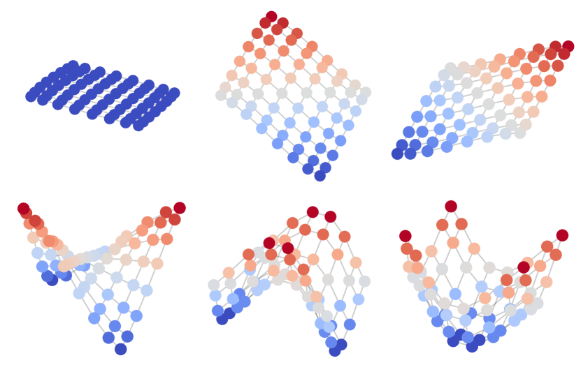
We finally mention that although our algorithm is motivated by the cSBM, it could have equivalently been motivated by ubiquitous low-dimensional graphs. In such graphs node labels are related to the low-dimensional coordinates, which are in turn given by the eigenvectors of the graph Laplacian; this is illustrated in Figure 3. If, for example, the labels are given by the sign of the first non-constant eigenfunction (the slowest-changing normal mode), our notion of alignment with $L=1$ clearly remains meaningful.

This also further motivates our terminology of resonance. In a purist sense, resonance is a dynamical phenomenon where driving a system with a frequency corresponding to an eigenvalue of the Laplacian yields a diverging response. Importantly, the shape of the response is then an eigenfunction. In a broad sense, resonance signifies alignment with Laplacian eigenfunctions, which are the natural modes. For graphs, this is closely related to alignment with eigenvectors of the adjacency matrix (it is equivalent for $d$-regular graphs). As Figure 2(b) shows, maximizing alignment between feature and graph spectra indeed leads to the largest response of the graph to the features.

4 Experiments

We evaluate JDR on both synthetic data generated from the cSBM and real-world benchmark datasets. Following the experimental setup from [8], we evaluate the performance for semi-supervised node classification with GNNs as the downstream algorithm in the transductive setting. We also adopt their data splits, namely the sparse splitting $2.5\%/2.5\%/95\%$ for training, validation and testing, respectively, or the dense splitting $60\%/20\%/20\%$. For each experimental result we perform $100$ runs with different random splits for training, validation and test data and report the average accuracy and the $95\%$-confidence interval calculated via bootstrapping with 1000 samples. All experiments are reproducible using the code provided.

Baselines. Following related work on rewiring [38], we use a graph convolution network (GCN) as our baseline downstream algorithm. To obtain a more comprehensive picture, we additionally evaluate the performance on the more recent and more powerful generalized PageRank graph neural network (GPRGNN) [8]. The latter learns a polynomial graph filter which enables it to perform strongly on heterophilic graphs. We compare our algorithm to batch Ollivier-Ricci flow (BORF) [30], the current state-of-the-art rewiring method. In this curvature-based rewiring method, edges are added in regions of negative curvature and removed for positive curvature. This is motivated by the fact that negative curvature indicates bottlenecks in the graph, which can lead to the so-called oversquashing of the messages passed along these edges. A positive curvature, on the other hand, indicates that there are so many edges in this area that messages could be oversmoothed, which is why edges are removed here. For the experiments on the cSBM, we additionally compare to the approximate message passing-belief propagation (AMP-BP) algorithm [12]. AMP-BP is an asymptotically optimal algorithm (in the large dimension limit) for unsupervised or semi-supervised community detection in the cSBM. This algorithm essentially relies on knowing the distribution of the cSBM and is thus not applicable to real-world graphs with unknown characteristics and complex features.

Hyperparameters. We use the hyperparameters from [8] for the GNNs unless stated otherwise and optimize the hyperparameters of JDR using a mixture of grid and random search on the validation set. Across all datasets, we use the top-$64$ values of $\tilde{\bm{A}}$ building a sparse, weighted graph and an interpolation to update the features $\tilde{\bm{X}}=\eta_{X_{2}}\tilde{\bm{X}}+(1-\eta_{X_{2}})\bm{X}$. For BORF, we tune its hyperparameters using a grid search within the given parameter range from the original paper. For both hyperparameter searches we use GCN and GPRGNN as the downstream models on $10$ runs with different random splits. A detailed list of all hyperparameters can be found in Appendix A.5 or in the code repository.

4.1 Results on Synthetic Data

We first test our method on data generated from the cSBM, as we can easily vary the SNR of the graph and the features to verify its denoising and rewiring capabilities. In recent work on GNNs [8, 40], the cSBM is increasingly used to evaluate the performance of semi-supervised node classification. The benefits of such an analysis have been emphasized in [12], especially in the sparse splitting regime. We focus on the weakly-supervised setting, i.e., the sparse splitting regime, since for dense splitting GPRGNN already almost achieves the performance of AMP-BP [12].

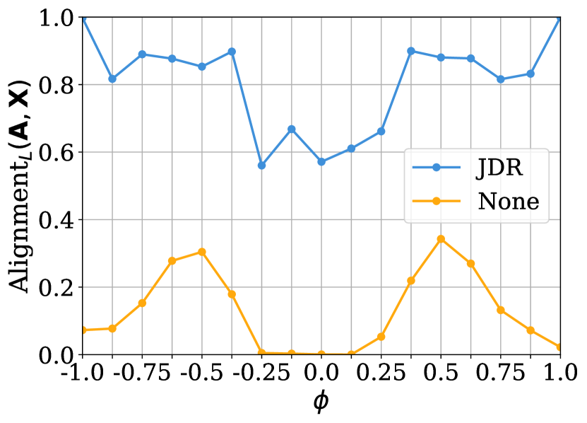
Does JDR maximize Alignment? Before discussing Figure 5 which shows the results of baselines and JDR for different values of $\phi$, we verify empirically that our alternating optimization algorithm indeed approximates solutions to (4). As shown in Figure 4, across different values of $\phi$, the quantity $\mathrm{Alignment}_{L}(\bm{A},\bm{X})$ improves significantly after running JDR. As we show next, this happens simultaneously with improvements in downstream performance, which lends credence to the intuitive reasoning that motivates our algorithm.

Figure 4: Alignment of the leading eigenspaces according to (3) for graphs from the cSBM with different $\phi$.

Heterophilic Regime. For $\phi<-0.25$, the predictions of GCN are only slightly better than random. GPRGNN performs much better, since it can learn higher order polynomial filters to deal with heterophily [8]. GCN +JDR outperforms the baseline by a very large margin; it handles heterophilic data well. Using JDR for GPRGNN further improves its already strong performance in this regime. Both GNNs benefit less from the denoising in the weakly heterophilic setting with $\phi\in\{-0.25,-0.125\}$ where they exhibit the worst performance across all $\phi$. Without any denoising, $\phi=0$ is the hardest setting. The difference between this and the weakly heterophilic regime is that “optimal denoising” for $\phi=0$ is straightforward, since all the information is contained in the node features. The baseline similarly perform poorly in this setting for both GNNs. We show similar findings for spectral clustering on the cSBM in Appendix A.3.3.

Weak Graph Regime. For $|\phi|\leq 0.25$, where the SNR of the graph is very low, both GNNs perform poorly. Intuitively, if the graph is very noisy, a GNN is a suboptimal model, since its message passing computations leverage the graph structure. A simple multilayer perceptron (MLP) baseline, using only the node features, outperforms GNNs in this setting, with all three approaches lagging far behind AMP-BP. Using JDR, we see significant performance increases for both GNN models which almost catch up with AMP-BP for $\phi=0$. With the denoised graph we can observe a clear advantage of the GNN. Although all information is available in the node features, the GNN with rewiring now clearly outperforms the MLP by a very large margin. We argue that this is because in the transductive setting with few labels available, the GNN generalizes much better.

Figure 5: Average accuracy across runs of the tested approaches on graphs from the cSBM with different values of $\phi$. The error bars indicate the $95\%$ confidence interval. JDR improves the performance for both GCN and GPRGNN across all $\phi$. The improvement is the most evident in the weak graph regime ($|\phi|\to 0$) and for GCN also in the heterophilic regime ($\phi<0$).

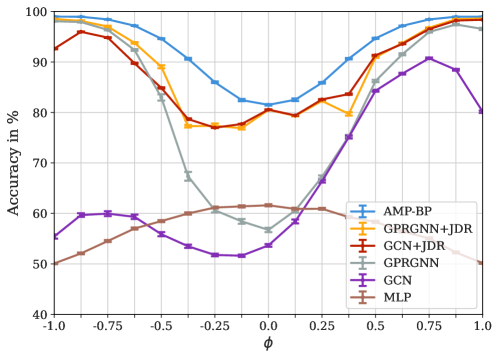
Homophilic Regime. For $\phi>0.25$ both GCN and GPRGNN perform similarly well, with GPRGNN achieving better results for $\phi\to 1.0$. With JDR preprocessing, they become much more comparable to each other and closer to AMP-BP. Even though the hyperparameters of JDR were tuned using only GCN as a downstream model, it improves the performance of GPRGNN also for all $\phi$. However, there is one noticeable outlier for GPRGNN at $\phi=0.375$. We suspect that since the performance without JDR is the same for GCN and GPRGNN here, the performance with JDR is more optimized for GCN, resulting in the outlier for GPRGNN. The general robustness to hyperparameter changes is also analyzed in detail in Appendix A.4.

4.2 Results on Real-World Data

We evaluate JDR on five common homophilic benchmarks datasets, namely the citation graphs Cora, CiteSeer, PubMed [34] and the Amazon co-purchase graphs Computers and Photo [27]. For heterophilic benchmark datasets we rely on the Wikipedia graphs Chameleon and Squirrel [33], the WebKB datasets Texas and Cornell used in [32] and the actor co-occurence network Actor [37]. Further details about the datasets are in Appendix A.2. Following [8], we evaluate the homophilic datasets in the sparse splitting staying close to the original setting of GCN [20] and the heterophilic datasets in dense splitting [32]. For additional results, we refer to Appendix A.3.

Homophilic Datasets. Table 1 shows the results of the GNNs with JDR compared to the baselines. Either GCN or GPRGNN with JDR achieves the best results. BORF, on the other hand, is not able to improve the performance of a GNN in this sparse setting, unlike in the experimental (dense) setting of the original paper. We suspect that oversmoothing and oversquashing, which BORF was designed to reduce, plays a less critical role in the sparse setting. With fewer labels available, it is also less likely that passing their information along the graph gets oversquashed at some point. The fact that GCN and GPRGNN with JDR perform similarly well here is also consistent with the results for cSBM.

Heterophilic Datasets. The results in Table 2 show that GCN +JDR can catch up significantly compared to GPRGNN, but in most cases GPRGNN +JDR performs better. This is in line with the findings for the cSBM. BORF also improves performance here in most cases, but is outperformed by JDR in all cases, often by a large margin. The out-of-memory error on Squirrel for BORF results from the computational complexity of the method. It is $\mathcal{O}(md^{3}_{\text{max}})$ [14] and the dataset has a large number of edges $m$ and a high maximum node degree $d_{\text{max}}$. The complexity of our method, on the other hand, is at best only weakly dependent on the node degree due to the spectral decomposition.

Table 1: Results on real-world homophilic datasets using the sparse splitting (2.5%/2.5%/95%): Mean accuracy across runs (%) $\pm\ 95\%$ confidence interval. Best average accuracy in bold. JDR achieves the best performance for both GCN and GPRGNN.

Method	Cora	CiteSeer	PubMed	Computers	Photo
GCN	$77.26$$\pm 0.35$	$67.16$$\pm 0.37$	$84.22$$\pm 0.09$	$84.42$$\pm 0.31$	$91.33$$\pm 0.29$
GCN+BORF	$77.23$$\pm 0.35$	$66.96$$\pm 0.38$	$84.22$$\pm 0.09$	$84.46$$\pm 0.30$	$91.26$$\pm 0.30$
GCN+JDR	$79.96$$\pm 0.26$	$\bm{69.35}$$\pm\bm{0.28}$	$84.79$$\pm 0.08$	$\bm{85.66}$$\pm\bm{0.36}$	$92.52$$\pm 0.23$
GPRGNN	$79.65$$\pm 0.33$	$67.50$$\pm 0.35$	$84.33$$\pm 0.10$	$84.06$$\pm 0.48$	$92.01$$\pm 0.41$
GPRGNN+BORF	$79.43$$\pm 0.30$	$67.48$$\pm 0.36$	$84.36$$\pm 0.10$	$84.08$$\pm 0.43$	$92.11$$\pm 0.38$
GPRGNN+JDR	$\bm{80.77}$$\pm\bm{0.29}$	$69.17$$\pm 0.30$	$\bm{85.05}$$\pm\bm{0.08}$	$84.77$$\pm 0.35$	$\bm{92.68}$$\pm\bm{0.25}$

Table 2: Results on real-world heterophilic dataset using the dense splitting (60%/20%/20%): Mean accuracy across runs (%) $\pm\ 95\%$ confidence interval. Best average accuracy in bold. OOM indicates an out-of-memory error. JDR achieves the best performance for both GCN and GPRGNN.

Method	Chameleon	Squirrel	Actor	Texas	Cornell
GCN	$67.65$$\pm 0.42$	$57.94$$\pm 0.31$	$34.00$$\pm 0.31$	$75.62$$\pm 1.12$	$64.68$$\pm 1.25$
GCN+BORF	$67.78$$\pm 0.43$	OOM	$33.95$$\pm 0.31$	$76.66$$\pm 1.10$	$68.72$$\pm 1.11$
GCN+JDR	$69.76$$\pm 0.50$	$\bm{61.76}$$\pm\bm{0.39}$	$40.47$$\pm 0.31$	$85.12$$\pm 0.74$	$84.51$$\pm 1.06$
GPRGNN	$69.15$$\pm 0.51$	$53.44$$\pm 0.37$	$39.52$$\pm 0.22$	$92.82$$\pm 0.67$	$87.79$$\pm 0.89$
GPRGNN+BORF	$69.44$$\pm 0.56$	OOM	$39.55$$\pm 0.20$	$93.53$$\pm 0.68$	$88.83$$\pm 1.06$
GPRGNN+JDR	$\bm{71.00}$$\pm\bm{0.50}$	$60.62$$\pm 0.38$	$\bm{41.89}$$\pm\bm{0.24}$	$\bm{93.85}$$\pm\bm{0.54}$	$\bm{89.45}$$\pm\bm{0.84}$

5 Conclusion and Limitations

Our experimental results clearly show that spectral resonance is a powerful principle on which to build graph and feature denoising algorithms. JDR consistently outperforms existing rewiring methods [38, 30] on both synthetic and real-world graph datasets. The smaller performance gains of GPRGNN suggest that this more powerful GNN is already able to leverage the complementary spectra of graphs and features to some extent, especially for heterophilic graphs.

Still, we should emphasize that the existing rewiring methods only use the graph, not the features. A direct comparison is thus not fair, as JDR cannot be used at all without features. Nonetheless, we have proposed the first generally applicable algorithm for cases where such information is available.

On a meta level, our results suggest that noise in real-world graph data is an important limiting factor for the performance of GNNs. It would therefore also be interesting to see whether feature-agnostic rewiring from a denoising perspective, for example using link prediction, could be used to improve the downstream performance. A related idea that we tried, but could not get to work well, is combining existing geometric rewiring algorithms with JDR. Intuitively, there should be a way to benefit from both removing noise and facilitating computation, but we have to leave that for future work.

Another possible limitation of our work is that it is based on the cSBM and therefore assumes that the features are linear as in a GMM, which makes a linear classifier optimal. If the class boundaries are highly nonlinear, this is no longer true, and the spectrum of $\bm{X}$ may need to be “linearized”, e.g. via Laplacian eigenmaps or diffusion maps. Still, the results with real-world data show that the cSBM model is already highly transferable, suggesting that the high-dimensional features in real-world graph datasets are often quite linear.

Finally, this work is based on heuristic reasoning from spectral graph theory, and our focus has been on a strong algorithmic implementation. While Figure 4 shows that JDR indeed maximizes alignment according to (3), and the experimental results show that this leads to better performance, it remains an outstanding theoretical question whether anything can be said for semi-supervised node classification in this case.

Appendix A Appendix

A.1 The JDR algorithm

Algorithm 1 Joint Denoising and Rewiring

1:procedure Rewire($\bm{X},\bm{A}$) $\triangleright$ For Denoise just exchange $\bm{X}$ and $\bm{A}$

2:     $\bm{X}=\bm{U}\bm{\Sigma}\bm{W}^{T}$

3:     $\bm{A}=\bm{V\Lambda}\bm{V}^{T}$

4:     for $i$ in $\text{range}(L_{A})$ do $\triangleright$ Loop over $L_{A}$ eigenvectors in $\bm{A}$

5:         $\bm{v}_{a}\leftarrow\bm{V}[:,i]$

6:         for $j$ in $\text{range}(L_{A})$ do $\triangleright$ Loop over $L_{A}$ eigenvectors in $\bm{X}$

7:              $\bm{u}_{x}\leftarrow\bm{U}[:,j]$

8:              $\theta\leftarrow\langle\bm{u}_{x},\bm{v}_{a}\rangle$ $\triangleright$ Find angle between eigenvectors

9:              if $|\theta|>|\theta_{\text{max}}|$ then

10:                  $\theta_{\text{max}}\leftarrow\theta$

11:                  $\bm{u}_{x}^{\text{max}}\leftarrow\bm{u}_{x}$

12:              end if

13:         end for

14:         $\tilde{\bm{V}}[:,i]\leftarrow(1-\eta_{A})\bm{v}_{a}+\eta_{A}\text{sign}(\theta_{\text{{max}}})\bm{u}_{x}^{\text{max}}$ $\triangleright$ Interpolation between eigenvectors

15:     end for

16:     $\tilde{\bm{A}}\leftarrow\tilde{\bm{V}}\bm{\Lambda}\tilde{\bm{V}}^{T}$

17:end procedure

18:$\tilde{\bm{X}},\tilde{\bm{A}}\leftarrow\bm{X},\bm{A}$

19:for $i$ in $\text{range}(\text{K})$ do $\triangleright$ Main loop

20:     $\bm{X}^{\prime}\leftarrow\textsc{Denoise}(\tilde{\bm{X}},\tilde{\bm{A}})$

21:     $\bm{A}^{\prime}\leftarrow\textsc{Rewire}(\tilde{\bm{X}},\tilde{\bm{A}})$

22:     $\tilde{\bm{X}},\tilde{\bm{A}}\leftarrow\bm{X}^{\prime},\bm{A}^{\prime}$

23:end for

24:$\tilde{\bm{X}}=\textsc{Update\_X}(\bm{X},\tilde{\bm{X}})$ $\triangleright$ Sparsify and binarize if needed

25:$\tilde{\bm{A}}=\textsc{Update\_A}(\bm{A},\tilde{\bm{A}})$

Table 3: Properties of the real-world benchmark datasets. For directed graphs we transform the graph to undirected in all experiments. $\mathcal{H}(\mathcal{G})$ indicates the homophily measure.

Dataset	Classes	Features	Nodes	Edges	Directed	$\mathcal{H}(\mathcal{G})$
Cora	$7$	$1433$	$2708$	$5278$	False	$0.810$
Citeseer	$6$	$3703$	$3327$	$4552$	False	$0.736$
PubMed	$3$	$500$	$19717$	$44324$	False	$0.802$
Computers	$10$	$767$	$13752$	$245861$	False	$0.777$
Photo	$8$	$745$	$7650$	$119081$	False	$0.827$
Chameleon	$6$	$2325$	$2277$	$31371$	True	$0.231$
Squirrel	$5$	$2089$	$5201$	$198353$	True	$0.222$
Actor	$5$	$932$	$7600$	$26659$	True	$0.219$
Texas	$5$	$1703$	$183$	$279$	True	$0.087$
Cornell	$5$	$1703$	$183$	$277$	True	$0.127$

A.2 Datasets

Table 3 shows the properties of the real-world datasets used. We also provide the homophily measure $\mathcal{H}(\mathcal{G})$ proposed in [32], which we compute using the build-in function of Pytorch Geometric [15]. For the cSBM, following [8], we choose $N=5000$, $F=2000$ and thus have $\gamma=\frac{N}{F}=2.5$. Since the threshold to recover communities in cSBM is $\lambda^{2}+\mu^{2}/\gamma>1$ [10], we use a margin such that $\lambda^{2}+\mu^{2}/\gamma=1+\epsilon$. We choose $\epsilon=3.25$ in all our experiments to be above the detection threshold and $d=5$ to obtain a sparse graph to be close to the properties of real-world graphs. From the recovery threshold, we can parameterize the resulting arc of an ellipse with $\lambda\geq 0$ and $\mu\geq 0$ using $\phi=\arctan(\lambda\sqrt{\gamma}/\mu)$. Table 4 shows the parameters $\mu^{2}$ and $\lambda$ and the homophily measure $\mathcal{H}(\mathcal{G})$for the different values of $\phi$.

Table 4: Properties of the synthetic datasets generated from the cSBM with $\epsilon=3.25$. $\mathcal{H}(\mathcal{G})$ indicates the homophily measure.

$\boldsymbol{\phi}$	$\mu^{2}$	$\lambda$	$\mathcal{H}(\mathcal{G})$
$-1.0$	$0.0$	$-2.06$	$0.039$
$-0.875$	$0.40$	$-2.02$	$0.049$
$-0.75$	$1.56$	$-1.90$	$0.076$
$-0.625$	$3.28$	$-1.71$	$0.119$
$-0.5$	$5.31$	$-1.46$	$0.170$
$-0.375$	$7.35$	$-1.15$	$0.241$
$-0.25$	$9.07$	$-0.79$	$0.325$
$-0.125$	$10.22$	$-0.40$	$0.408$
$0.0$	$10.63$	$0.0$	$0.496$
$0.125$	$10.22$	$0.40$	$0.583$
$0.25$	$9.07$	$0.79$	$0.671$
$0.375$	$7.35$	$1.15$	$0.751$
$0.5$	$5.31$	$1.46$	$0.837$
$0.625$	$3.28$	$1.71$	$0.879$
$0.75$	$1.56$	$1.90$	$0.925$
$0.875$	$0.40$	$2.02$	$0.955$
$1.0$	$0.0$	$2.06$	$0.963$

A.3 Additional Results

We provide a number of additional experiments which did not fit in the main text. These include a comparison of our method to diffusion improves graph learning (DIGL)[16], results for the homophilic datasets in the dense splitting and results for synthetic and real-world data using spectral clustering with and w/o JDR.

(a)

(b)

Figure 6: Comparison of DIGL [16] and JDR on the cSBM datasets in the sparse splitting. Results for (8(a)) GCN and (8(b)) GPRGNN as downstream models. The error bars indicate the $95\%$ confidence interval. As expected, DIGL is not really able to improve the performance of the GNNs in the heterophilic regime. It achieves the greatest improvement in the weak-graph regime and for strongly homophilic graphs, especially using GCN as downstream model. Another interesting observation is that for GCN and $\phi<0.25$ the curve of MLP corresponds exactly to the one of GCN +DIGL. The reason for this is that the hyperparameters found for DIGL ensure that the graph is ignored ($\alpha=1.0$), which means that the GCN then collapses to a simple MLP. For the more powerfull GPRGNN, on the other hand, DIGL is generally hardly able to improve performance, while JDR clearly increases the performance across all $\phi$.

A.3.1 Comparison to DIGL

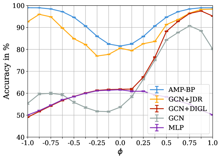
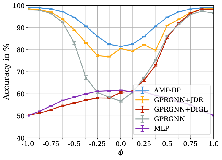
We compare our method to DIGL [16]. We use the personalized PageRank (PPR) diffusion kernel and the same top-$64$ values sparsening method as in JDR in all experiments. For tuning the random teleport probability $\alpha$, we perform a grid search on values between $0.0$ and $1.0$ using the validation set on 10 random splits. Figure 6 shows the results for DIGL on the synthetic datasets from the cSBM. Table 5 shows the results on the real-world homophilic datasets in the sparse splitting and Table 6 on the heterophilic datasets in the dense splitting. Here, in addition to the individual results for JDR and DIGL, the results for a combination of the two methods are also shown. For this purpose, the graph was first denoised with JDR and then diffused with DIGL. To do this, we fixed the hyperparameters of JDR and then tuned the parameter $\alpha$ of DIGL.

Homophilic datasets. For the homophilic datasets, both DIGL and JDR can improve the results when GCN is used as a downstream model. Still, DIGL is outperformed by JDR on four out the five datasets. Interestingly, the two methods can be combined on three of the five data sets to achieve even better results. This indicates that the two methods use a distinct way of performing rewiring in this case and a combination therefore can further increase accuracy. The picture is somewhat different for GPRGNN as a downstream model. The improvements for DIGL are significantly smaller here, whereas JDR shows clear improvements across all datasets. This suggests that a more powerful GNN architecture benefits less from DIGL, while JDR can still improve it even further. A combination of the two methods does not lead to an increase in performance here. Although the performance is still significantly better compared to no rewiring or just DIGL, JDR alone usually performs better.

Table 5: Comparison of DIGL and JDR on real-world homophilic dataset using the sparse splitting: Mean accuracy (%) $\pm\ 95\%$ confidence interval. Best average accuracy in bold.

Method	Cora	CiteSeer	PubMed	Computers	Photo
GCN	$77.26$$\pm 0.35$	$67.16$$\pm 0.37$	$84.22$$\pm 0.09$	$84.42$$\pm 0.31$	$91.33$$\pm 0.29$
GCN+DIGL	$79.27$$\pm 0.26$	$68.03$$\pm 0.33$	$84.60$$\pm 0.09$	$\bm{86.00}$$\pm\bm{0.24}$	$92.00$$\pm 0.23$
GCN+JDR	$79.96$$\pm 0.26$	$\bm{69.35}$$\pm\bm{0.28}$	$84.79$$\pm 0.08$	$85.66$$\pm 0.36$	$92.52$$\pm 0.23$
GCN+JDR+DIGL	$\bm{80.48}$$\pm\bm{0.26}$	$69.19$$\pm 0.29$	$\bm{84.83}$$\pm\bm{0.10}$	$84.78$$\pm 0.34$	$\bm{92.69}$$\pm\bm{0.22}$
GPRGNN	$79.65$$\pm 0.33$	$67.50$$\pm 0.35$	$84.33$$\pm 0.10$	$84.06$$\pm 0.48$	$92.01$$\pm 0.41$
GPRGNN+DIGL	$79.77$$\pm 0.30$	$67.50$$\pm 0.35$	$84.72$$\pm 0.10$	$\bm{86.25}$$\pm\bm{0.28}$	$92.31$$\pm 0.25$
GPRGNN+JDR	$\bm{80.77}$$\pm\bm{0.29}$	$69.17$$\pm 0.30$	$\bm{85.05}$$\pm\bm{0.08}$	$84.77$$\pm 0.35$	$\bm{92.68}$$\pm\bm{0.25}$
GPRGNN+JDR+DIGL	$80.55$$\pm 0.27$	$\bm{69.47}$$\pm\bm{0.27}$	$84.87$$\pm 0.10$	$85.98$$\pm 0.21$	$92.67$$\pm 0.27$

Table 6: Comparison of DIGL and JDR on real-world heterophilic dataset using the dense splitting: Mean accuracy (%) $\pm\ 95\%$ confidence interval. Best average accuracy in bold.

Method	Chameleon	Squirrel	Actor	Texas	Cornell
GCN	$67.65$$\pm 0.42$	$57.94$$\pm 0.31$	$34.00$$\pm 0.31$	$75.62$$\pm 1.12$	$64.68$$\pm 1.25$
GCN+DIGL	$58.04$$\pm 0.48$	$39.64$$\pm 0.34$	$39.57$$\pm 0.29$	$\bm{91.05}$$\pm\bm{0.73}$	$\bm{88.49}$$\pm\bm{0.74}$
GCN+JDR	$\bm{69.76}$$\pm\bm{0.50}$	$\bm{61.76}$$\pm\bm{0.39}$	$\bm{40.47}$$\pm\bm{0.31}$	$85.12$$\pm 0.74$	$84.51$$\pm 1.06$
GCN+JDR+DIGL	$66.06$$\pm 0.43$	$36.62$$\pm 0.29$	$40.30$$\pm 0.27$	$88.90$$\pm 0.73$	$88.06$$\pm 0.77$
GPRGNN	$69.15$$\pm 0.51$	$53.44$$\pm 0.37$	$39.52$$\pm 0.22$	$92.82$$\pm 0.67$	$87.79$$\pm 0.89$
GPRGNN+DIGL	$66.57$$\pm 0.46$	$42.98$$\pm 0.37$	$39.61$$\pm 0.21$	$91.11$$\pm 0.72$	$88.06$$\pm 0.81$
GPRGNN+JDR	$\bm{71.00}$$\pm\bm{0.50}$	$\bm{60.62}$$\pm\bm{0.38}$	$\bm{41.89}$$\pm\bm{0.24}$	$\bm{93.85}$$\pm\bm{0.54}$	$\bm{89.45}$$\pm\bm{0.84}$
GPRGNN+JDR+DIGL	$70.07$$\pm 0.44$	$59.37$$\pm 0.35$	$41.57$$\pm 0.20$	$91.52$$\pm 0.70$	$87.77$$\pm 1.81$

Table 7: Comparison of DIGL, BORF and JDR on real-world homophilic datasets using the dense splitting: Mean accuracy (%) $\pm\ 95\%$ confidence interval. Best average accuracy in bold.

Method	Cora	CiteSeer	PubMed	Computers	Photo
GCN	$88.14$$\pm 0.27$	$79.02$$\pm 0.25$	$86.14$$\pm 0.10$	$89.03$$\pm 0.12$	$94.07$$\pm 0.10$
GCN+BORF	$88.18$$\pm 0.24$	$79.17$$\pm 0.24$	$86.14$$\pm 0.10$	$89.14$$\pm 0.11$	$94.00$$\pm 0.10$
GCN+DIGL	$88.74$$\pm 0.28$	$79.13$$\pm 0.27$	$\bm{87.81}$$\pm\bm{0.09}$	$\bm{90.34}$$\pm\bm{0.12}$	$\bm{94.87}$$\pm\bm{0.10}$
GCN+JDR	$\bm{88.76}$$\pm\bm{0.25}$	$\bm{80.25}$$\pm\bm{0.27}$	$86.20$$\pm 0.10$	$88.93$$\pm 0.13$	$94.20$$\pm 0.08$
GPRGNN	$88.57$$\pm 0.0.25$	$79.42$$\pm 0.30$	$89.16$$\pm 0.15$	$88.95$$\pm 0.18$	$94.49$$\pm 0.11$
GPRGNN+BORF	$88.56$$\pm 0.27$	$79.39$$\pm 0.31$	$89.04$$\pm 0.18$	$88.90$$\pm 0.19$	$94.52$$\pm 0.10$
GPRGNN+DIGL	$88.49$$\pm 0.24$	$79.62$$\pm 0.29$	$88.89$$\pm 0.16$	$\bm{90.15}$$\pm\bm{0.14}$	$94.27$$\pm 0.10$
GPRGNN+JDR	$\bm{89.33}$$\pm\bm{0.25}$	$\bm{81.00}$$\pm\bm{0.28}$	$\bm{89.24}$$\pm\bm{0.15}$	$87.35$$\pm 0.32$	$\bm{94.78}$$\pm\bm{0.08}$

Heterophilic datasets. Since DIGL rewires the graph by adding edges between nodes with short diffusion distance, it is expected to perform poorly on the heterophilic datasets. The results using GCN show that this is only true for Chameleon and Squirrel, while for Actor, Texas and Cornell there are still considerable improvements. For the datasets Texas and Cornell, DIGL even achieve the best results. JDR, on the other hand, improves performance across datasets and GNNs. The reason for DIGL’s good performance on these datasets is a limitation of GCN. Since it can only approximate low-pass graph filters it is hard to deal with the heterophilic property of these datasets in general. If you simply use a MLP instead, which only uses the node features as input, you can achieve similar or sometimes even better results (see [8]). Looking at the values of the random teleporting probability $\alpha$ found by hyperparameter search for DIGL, they are $1.0$ for these three datasets. This means that the resulting graph is evenly connected everywhere and has small weights. In this case, GCN largely ignores the graph and thus performs very similarly to an MLP. This is also in line with the finding on the cSBM in Figure 6(a). However, we can also see that this does no longer works for GPRGNN, because this more powerful GNN is able to make better use of these complex graph structures. It can learn high-pass graph filters to leverage the heterophilic graph information and thus surpass the performance of a simple MLP. Consequently, ignoring the graph does not improve the performance, which is why DIGL cannot improve performance in this setting. JDR, on the other hand, can still achieve an improvement across all datasets. A combination of DIGL and JDR is generally not particularly useful in this scenario.

A.3.2 Homophilic Datasets in the Dense Splitting

Table 7 shows the results of of DIGL, BORF and JDR on real-world homophilic datasets using the dense splitting. The improvements of rewiring are smaller overall compared to the sparse splitting, but all three methods are able to improve it in most cases. With GCN as the downstream model, DIGL now performs best. JDR can still achieve the best result on two out of five data sets. When using GPRGNN as downstream model, JDR performs best four out of five datasets. DIGL and BORF, on the other hand, are not able to improve the performance in most cases. This suggests that a more powerful GNN architecture benefits less from DIGL or BORF, while JDR can still improve it even further. The computer dataset is an exception for both downstream GNNs, JDR is not really able to improve the performance at all, while DIGL can clearly improve it.

A.3.3 Spectral Clustering

In addition to the GNNs as a downstream algorithm, we also experimente with spectral clustering (SC). Spectral clustering either works with an existing graph, or a k-nearest neighbor graph is created from given (high-dimensional) node features. Then the $k$ largest eigenvectors of the graph are calculated (the first one is usually omitted as it is a constant vector) and their entries are then used as coordinates for a k-means clustering of the nodes into $k$ classes. We show that JDR using the hyperparameters found with GCN as a downstream model, improves the performance of a spectral clustering algorithm acting directly on $\bm{A}$ or $\bm{X}$. This indicates a close connection between GCNs and spectral clustering such that a good denoised graph for GCN is also a good graph for spectral clustering. Intuitively, since spectral clustering is related to the graph cut, this means that in this case the classes are connected with fewer edges, making them easier to cluster based on the cut.

(a)

(b)

Figure 7: Separate results for using spectral clustering on a rewriting only $\bm{A}$ (7(a)) and denoising only $\bm{X}$ (7(b)) compared to full JDR. Note that for $\phi\in\{0.5,0.625,0.875\}$ we had to use additional graphs generated using cSBM with an average node degree of $d=10$ for spectral clustering of $\bm{A}$ to work in general and for $\phi=0.875$ also for JDR. The reason for this is that the graph is very sparse so it is not necessarily connected such that there is no guarantee that spectral clustering works. However a larger node degree does not improve the performance of spectral clustering in general, while it may for GNNs.

Table 8: Results on real homophilic datasets using spectral clustering: Mean accuracy (%) and best result in bold. Here, all methods use the hyperparameters found using GCN as downstream algorithm.

Method	Cora	CiteSeer	Pubmed	Computers	Photo
SC(A)	$33.83$	$24.16$	$58.94$	$37.35$	$30.58$
SC(A)+BORF	$35.01$	$25.22$	$58.90$	$37.35$	$33.37$
SC(A)+DIGL	$29.54$	$22.18$	$59.65$	$61.55$	$25.41$
SC(A)+JDR	67.76	63.36	$\bm{72.90}$	$\bm{62.29}$	$\bm{65.67}$
SC(X)	$29.76$	$45.57$	$60.45$	$28.53$	$48.46$
SC(X)+JDR	34.68	45.90	$\bm{60.47}$	$\bm{28.55}$	$\bm{48.58}$

Table 9: Results on real heterophilic datasets using spectral clustering: Mean accuracy (%) and best result in bold. Here, all methods use the hyperparameters found using GCN as downstream algorithm.

	Chameleon	Squirrel	Actor	Texas	Cornell
SC(A)	$31.71$	$22.40$	$25.92$	$48.09$	$39.89$
SC(A)+BORF	$31.97$	OOM	$25.97$	$\bm{56.83}$	$43.17$
SC(A)+DIGL	$\bm{32.06}$	$\bm{22.69}$	$25.91$	$43.72$	$40.44$
SC(A)+JDR	$31.36$	$22.15$	$\bm{28.63}$	$52.46$	$\bm{44.26}$
SC(X)	$23.54$	$20.17$	$\bm{31.01}$	$49.18$	$45.36$
SC(X)+JDR	24.59	21.03	$23.99$	$\bm{55.74}$	$\bm{49.73}$

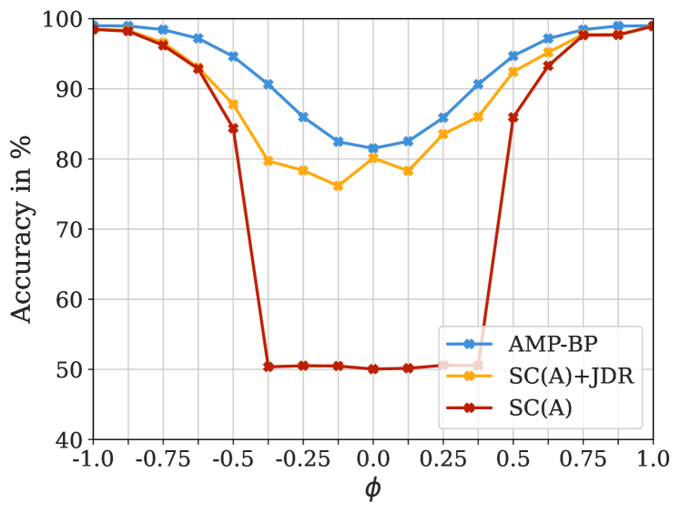
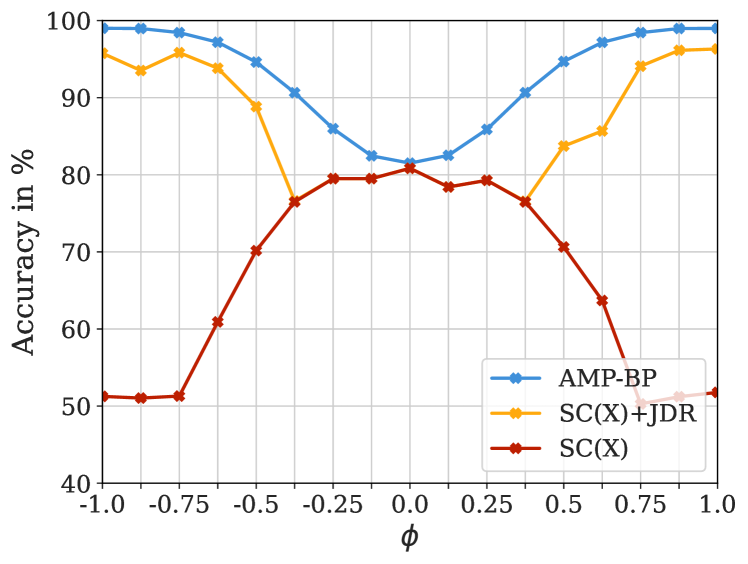
cSBM. Figure 7 displays the results of spectral clustering with and w/o JDR. Figure 7(a) indicates the expected behavior that spectral clustering using $\bm{A}$ performs particularly poorly in the weak graph regime, since in this case there is hardly any information about the labels in $\bm{A}$. By using JDR, this limitation is completely removed and the performance is close to AMP-BP across all $\phi$. The rewired graph now contains more information about the labels, which was previously only available in $\bm{X}$. For spectral clustering of $\bm{X}$ in Figure 7(b), the relation is exactly the other way around. In the strong heterophilic or homophilic regime the performance is poor since most information is contained in the graph structure. Using JDR this limitation is removed and the performance becomes closer to AMP-BP across all $\phi$. Although a slight denoising of $\bm{X}$ by $\bm{A}$ would be possible for $\phi=\pm 0.375$, there is no performance advantage here and these settings now show the weakest performance across all $\phi$.

Real-world Datasets. For the real world datasets, we compare the spectral clustering of $\bm{A}$ using the different rewiring methods BORF, DIGL and JDR. For the spectral clustering of $\bm{X}$ we can only evaluate JDR. Again we use the hyperparameters found using GCN as downstream model. The results in Table 8 on homophilic datasets show a significant benefit of using JDR across all datasets. BORF and DIGL are also able to improve the performance in some settings but not very consistently. There are also performance improvements across all datasets for the spectral clustering of $\bm{X}$ with JDR, but these are significantly smaller. This indicates that the rewiring of the graph has a significantly greater influence on performance here than the denoising of the features.

Table 9 shows the results for the heterophlic datasets. The results here are much more inconsistent. It is striking that DIGL improves Chameleon and Squirrel, while it has actually worsened performance for GCN. BORF can improve the performance on Texas and Cornell by a large margin, although DIGL and JDR perform better with the GCN. For the results of JDR, it is worth looking at them together with the spectral clustering of $\bm{X}$. On Chameleon and Squirrel the performance decreases for $\bm{A}$ but clearly increases for $\bm{X}$. On Texas and Cornell it is improved in all cases, but on $\bm{A}$ not as strongly as for BORF. On Actor, the performance for $\bm{X}$ has dropped, while JDR is also the only method that really improves the result for $\bm{A}$. To summarize, the improvements for JDR can be assigned to one of the two sources of information, either $\bm{A}$ or $\bm{X}$, for each dataset.

(a)

(b)

Figure 8: Separate results for rewiring only $\bm{A}$ and denoising only $\bm{X}$ compared to full JDR. Results for (8(a)) GCN and (8(b)) GPRGNN. The error bars indicate the $95\%$ confidence interval.

A.4 Ablations

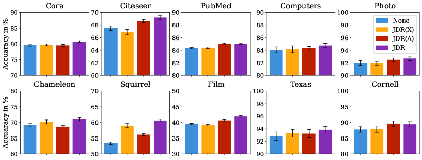
We perform several ablations of our method to investigate what happens in different scenarios and what effects changes in parameters have. First, we present our ablations of the JDR method. We show separate results for denoising only the graph JDR (A) or the features JDR (X) using the GNNs on the cSBM and real-world data. Also, we show several ablations of the hyperparameters of JDR. We therefore use a dataset created from cSBM, the homophilic dataset Cora and the heterophilic dataset Chameleon. Ablations on the real-world datasets are performed for all hyperparameters of JDR and show its robustness to change in these parameters.

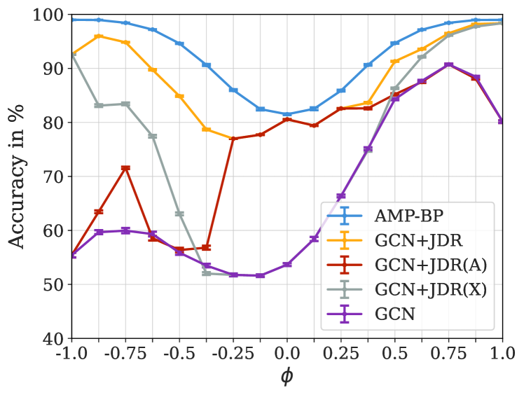
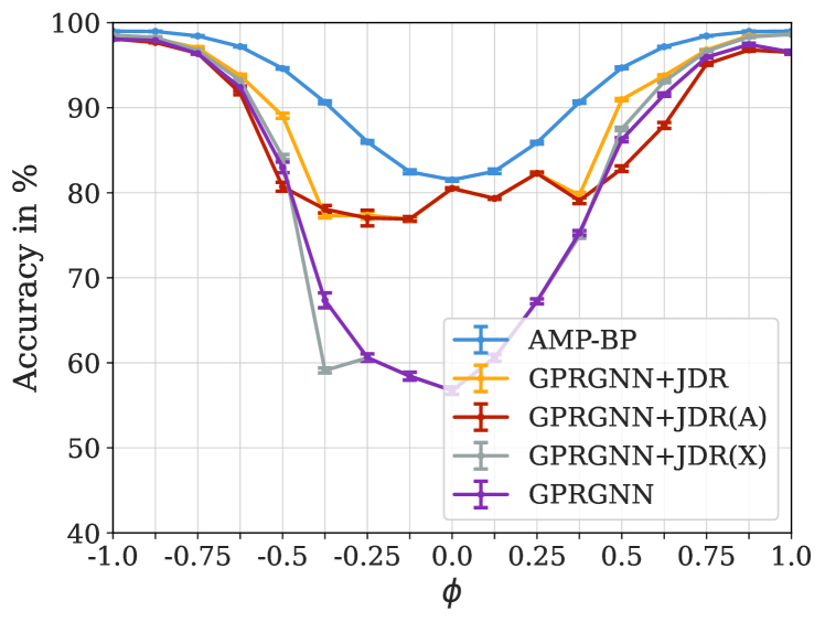
JDR. The main motivation for these ablations is to show how much impact the denoising of $\bm{A}$ and $\bm{X}$ respectively have on the results for a dataset and how big the additional benefit is to do this jointly. Therefore we look at the results if we denoise only the graph JDR (A) or the features JDR (X). Doing this for the cSBM in Figure 8, we can observe the expected behavior, which is particularly pronounced for GCN in Figure 8(a). In the weak graph regime, the performance increase results purely from denoising $\bm{A}$, so JDR (A) achieves the same performance as JDR. The same holds for JDR (X) in the strong homophilic regime and for $\phi=-1.0$. In the remaining intermediate regimes, we can often observe a performance benefit of both JDR (A) and JDR (X), which becomes much stronger when we combine both. This benefit of combining both is particularly pronounced for $\phi=-0.375$, where JDR (X) alone even reduces performance, while JDR clearly improves performance. In Figure 8(b), we can basically observe the same behavior, but less strongly pronounced. Moreover, it happens in several cases here, again especially in the intermediate regime, that the performance is reduced by JDR (X), but improved for the joint denoising.

Figure 9: Average accuracy of GCN on all real-world datasets tested for denoising only the features JDR (X), rewiring only the graph JDR (A) and joint denoising and rewiring JDR.

Figure 10: Average accuracy of GPRGNN on all real-world datasets tested for denoising only the features JDR (X), rewiring only the graph JDR (A) and joint denoising and rewiring JDR. It can be observed that for most datasets, the major improvement is achieved by JDR (A). Only for Squirrel and Chameleon it is JDR (X). In most cases using JDR on both $\bm{X}$ and $\bm{A}$ achieves the best performance.

Table 10: Comparison for JDR using hyperparameters tuned on different downstream models. The "*" indicates that the hyperparameters of JDR where tuned using the same GNN as downstream model, no symbol mean that the respective other GNN model was used. Results on real-world homophilic datasets using sparse splitting (2.5%/2.5%/95%): Mean accuracy (%) $\pm\ 95\%$ confidence interval. Best average accuracy in bold.

Method	Cora	CiteSeer	PubMed	Computers	Photo	$\uparrow$Gain
GCN	$77.26$$\pm 0.35$	$67.16$$\pm 0.37$	$84.22$$\pm 0.09$	$84.42$$\pm 0.31$	$91.33$$\pm 0.29$	-
GCN+JDR*	$\bm{79.96}$$\pm\bm{0.26}$	$\bm{69.35}$$\pm\bm{0.28}$	$\bm{84.79}$$\pm\bm{0.08}$	$\bm{85.66}$$\pm\bm{0.36}$	$\bm{92.52}$$\pm\bm{0.23}$	$1.59$
GCN+JDR	$78.85$$\pm 0.29$	$69.11$$\pm 0.28$	$84.20$$\pm 0.09$	$85.61$$\pm 0.21$	$92.25$$\pm 0.25$	$1.13$
GPRGNN	$79.65$$\pm 0.33$	$67.50$$\pm 0.35$	$84.33$$\pm 0.10$	$84.06$$\pm 0.48$	$92.01$$\pm 0.41$	-
GPRGNN+JDR	$80.47$$\pm 0.33$	$68.94$$\pm 0.29$	$\bm{85.17}$$\pm\bm{0.09}$	$84.64$$\pm 0.25$	$92.64$$\pm 0.21$	$0.86$
GPRGNN+JDR*	$\bm{80.77}$ $\pm\bm{0.29}$	$\bm{69.17}$$\pm\bm{0.30}$	$85.05$$\pm 0.08$	$\bm{84.77}$$\pm\bm{0.35}$	$\bm{92.68}$$\pm\bm{0.25}$	$0.98$

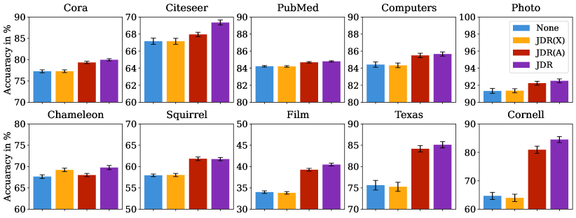
Figure 9 and Figure 10 show the same investigation for the real-world datasets using GCN and GPRGNN, respectively. In most cases, the greater performance gain results from JDR (A) and the joint denoising performs best. Only for the datasets Chameleon for both GNNs and Squirrel for GPRGNN, the denoising of $\bm{X}$ has the greater influence. Also the case where the denoising of $\bm{X}$ reduces the performance, but a joint denoising performs best, occurs here, e.g. for Citeseer or Cornell. Overall, this confirms that our method indeed performs joint denoising, especially when both graph and node contain relevant information both benefit from denoising.

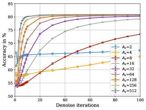
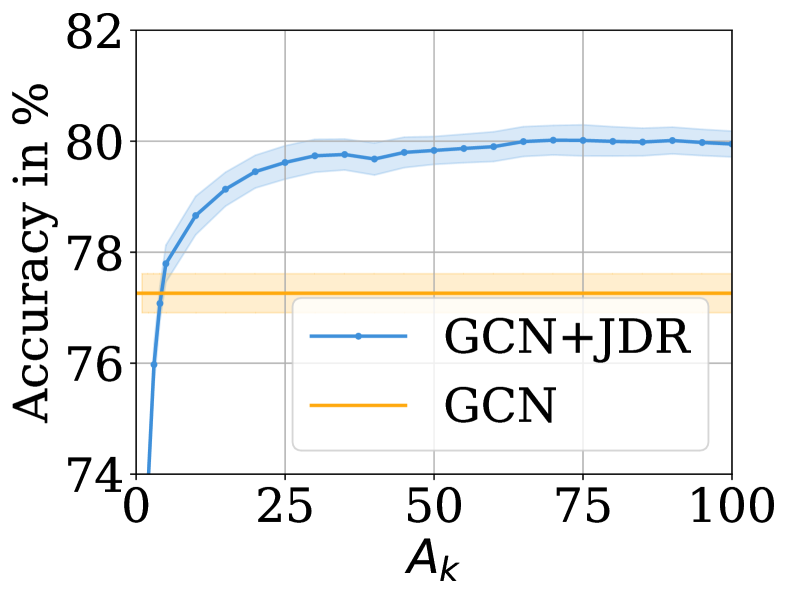
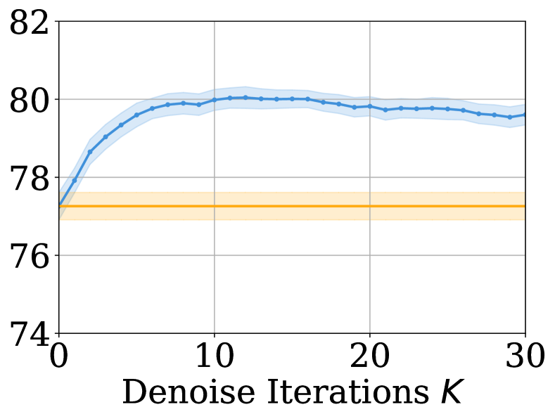
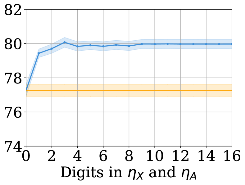
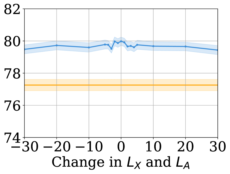
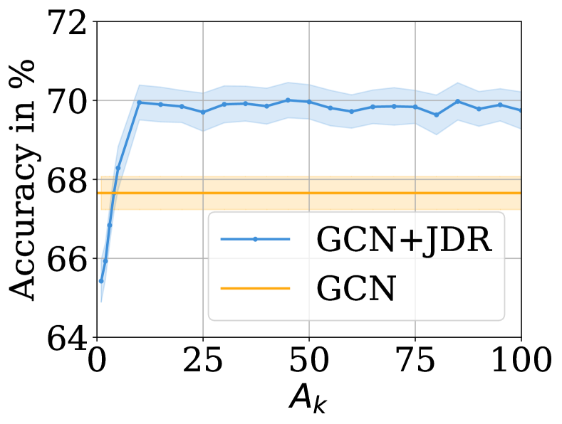
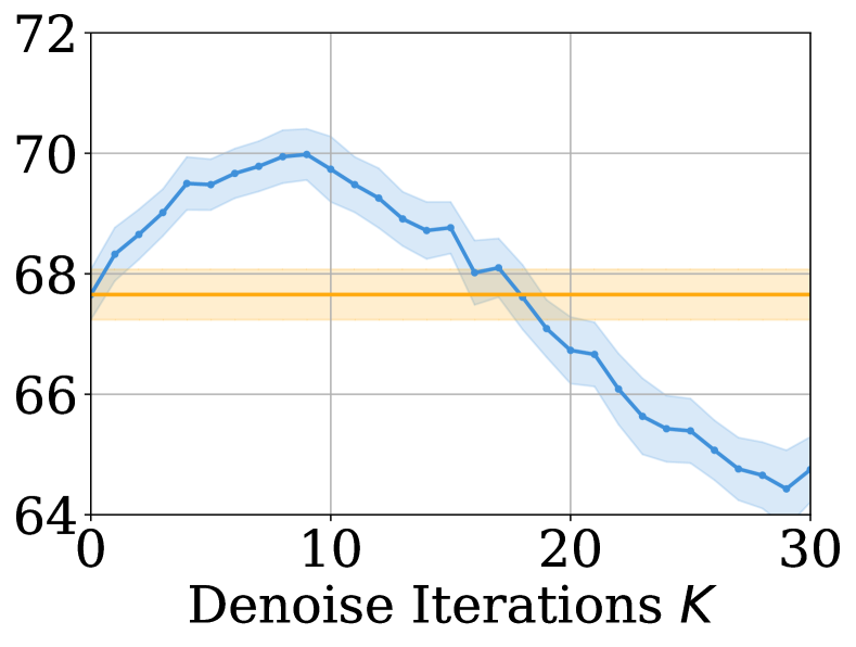
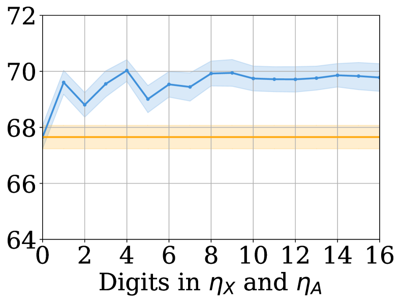
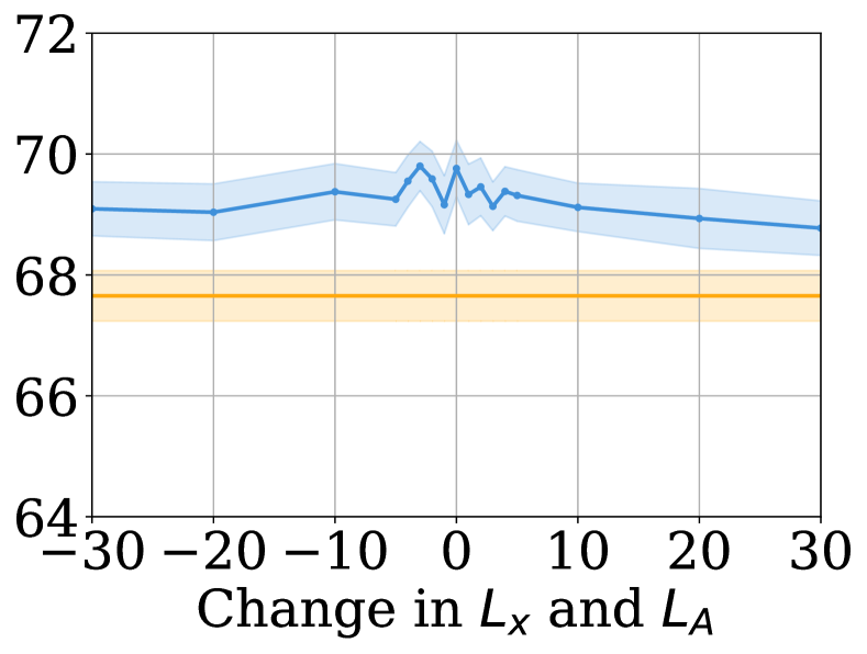
Hyperparameters. In Table 10 we show how the downstream GNN performs if JDR was tuned on a different downstream GNN. We use GCN and GPRGNN for this. The results show that the hyperparameters of JDR are quite robust to different GNN downstream models as it achieves similar gains using the respective other hyperparameters. Another way to show the robustness of JDR is to perform ablations of the actual hyperparameters. To do this, we first look at a data set generated from the cSBM and examine the influence of the number of denoising iterations $K$ and the number of entries of the adjacency matrix to be retained $A_{k}$. Figure 11 show the results of this study. As expected increase both results in better performance but will also increase the computational complexity. Based on this, we choose $A_{k}=64$ for all experiments as a good trade-off between computational and memory cost and accuracy over different numbers of denoising iterations. We also investigate this effect together with the rest of the hyperparameters for the real-world datasets Cora in Figure 12 and Chameleon in Figure 13. We again examine the number of denoising iterations $K$ and the number of entries of the adjacency matrix to be retained $A_{k}$. Additionally, we study the interpolation ratios $\eta_{X}$ and $\eta_{A}$ and the number of eigenvectors for the denoising $L_{X}$ and $L_{A}$. Both are analyzed relative to the value found by random search and for both $\bm{A}$ and $\bm{X}$ at the same time. For the interpolation ratios $\eta_{X}$ and $\eta_{A}$, we show the influence of using only a reduced number of digits of the best found value (0 corresponds to no denoising) and for the number of eigenvectors $L_{X}$ and $L_{A}$ we test different offsets (0 corresponding to the best value found using random search). Overall, we con observe a strong robustness to changes in the hyperparameters. Only the number of denoising iterations $K$ should not be too high for the heterophilic data set Chameleon.

Figure 11: Average accuracy of GCN on cSBM with $\phi=0.0$ for different numbers of denoise iterations and different numbers of entries $A_{k}$ to keep for each node in the rewired adjacency matrix. Error bars indicating the $95\%$ confidence interval over $100$ runs.

(a)

(b)

(c)

(d)

Figure 12: Ablations of GCN +JDR on the homophilic dataset Cora compared to the result for GCN. The light shaded ares indicate the $95\%$ confidence interval. Ablations on the number number of entries chosen per node for the adjacency $A_{k}$, the number of denoise iterations $K$, the number of interpolations digits for the $\eta$ values and the number of eigenvectors $L_{\square}$ used. All other parameters are kept constant. In all cases we can see that JDR is quite robust to changes in all of its hyperparameters.

(a)

(b)

(c)

(d)

Figure 13: Ablations of GCN +JDR on the heterophilic dataset Chameleon compared to the result for GCN. The light shaded ares indicate the $95\%$ confidence interval. We perfrom the same ablations as for Cora. In all cases except the number of denoising iterations, we can see that JDR is quite robust to changes in all of its hyperparameters.

A.5 Hyperparameters

In this section we list all the hyperparameters used for the experiments to ensure the reproducibility of the results. They are also included in the code. In all experiments we use the Adam optimizer and the standard early stopping after 200 epochs from [8]. Whenever we use a GCN, it uses two layers, a hidden dimension of $64$ and dropout with $0.5$. Whenever we use GPRGNN, we use a polynomial filter of order $10$ (corresponding to $10$ hops) and a hidden dimension of $64$. For JDR, we always keep the $64$ largest entries of the rewired adjacency matrix $\tilde{\bm{A}}$ per node. We justify this choice by the ablation in Figure 11.

cSBM. For synthetic data from the cSBM, we generally follow the hyperparameters from [8]. GCN uses a learning rate of $0.01$ and weight decay with $\lambda=0.0005$. GPRGNN also uses a $\lambda=0.0005$ and both use ReLU non-linearity. On homophilic graphs ($\phi\geq 0$), GPRGNN uses a learning rate of $0.01$, a weight initialization $\alpha=0.1$ and dropout with $0.5$. For heterophilic graphs, it uses a learning rate of $0.05$, $\alpha=1.0$ and dropout $0.7$. The hyperparameters for JDR on the cSBM are shown in Table 13. We only tuned them using GCN as a downstream model, so for GPRGNN +JDR we use the same ones.

Real-world Datasets. For the real-world datasets, the remaining hyperparameters for GCN are displayed in Table 11 and for GPRGNN in Table 12. The hyperparameters for JDR can be found in Table 14 and Table 15. For the rewiring method BORF, we list its hyperparameters in Table 16 and Table 17. For DIGL, we always use the PPR kernel and sparsify the result by keeping the top-$64$ values for a weighted adjacency matrix. The values for the random-teleport probabililty $\alpha$ are listed in Table 18 and Table 19.

Table 11: Hyperparameters of GCN. All models use $2$ layers, a hidden dimension of $64$ and dropout with $0.5$. Different type of weight decay and early stopping from [16] was used, if these provided a better performance then using the standard setting in [8]. The same holds for feature normalization, which was used by default in [8] for GPRGNN.

Dataset	Lr	Normalize $\bm{X}$	$\lambda_{1}$	$\lambda_{1}$ layer	Early stopping
Cora	$0.01$	False	$0.05$	First	GPRGNN
Citeseer	$0.01$	True	$0.0005$	All	GPRGNN
PubMed	$0.01$	True	$0.0005$	All	GPRGNN
Computers	$0.01$	False	$0.0005$	All	GPRGNN
Photo	$0.01$	False	$0.0005$	All	GPRGNN
Chameleon	$0.05$	True	$0.0$	All	DIGL
Squirrel	$0.05$	True	$0.0$	All	DIGL
Actor	$0.01$	False	$0.0005$	All	DIGL
Texas	$0.05$	True	$0.0005$	All	GPRGNN
Cornell	$0.05$	True	$0.0005$	All	GPRGNN

Table 12: Hyperparameters of GPRGNN. All models use $10$ hops and a hidden dimension of $64$.

Dataset	Lr	Normalize $\bm{X}$	$\alpha$	$\lambda_{1}$	Dropout	Early stopping
Cora	$0.01$	True	$0.1$	$0.0005$	$0.5$	GPRGNN
Citeseer	$0.01$	True	$0.1$	$0.0005$	$0.5$	GPRGNN
PubMed	$0.05$	True	$0.2$	$0.0005$	$0.5$	GPRGNN
Computers	$0.01$	False	$0.1$	$0.0005$	$0.5$	GPRGNN
Photo	$0.01$	False	$0.5$	$0.0$	$0.5$	GPRGNN
Chameleon	$0.05$	False	$1.0$	$0.0$	$0.7$	DIGL
Squirrel	$0.05$	True	$0.0$	$0.0$	$0.7$	GPRGNN
Actor	$0.01$	True	$0.9$	$0.0$	$0.5$	GPRGNN
Texas	$0.05$	True	$1.0$	$0.0005$	$0.5$	GPRGNN
Cornell	$0.05$	True	$0.9$	$0.0005$	$0.5$	GPRGNN

Table 13: Hyperparameters for GCN on the cSBM in the sparse splitting. For all homophilic datasets the eigenvalues are ordered by value and for all heterophilic datasets they are ordered by absolute value. In all setting we keep the $64$ largest entries of the rewired adjacency matrix $\tilde{\bm{A}}$ per node. Interpolation ratios $\eta$ are rounded to three digits from the best values found by the random search.

$\boldsymbol{\phi}$	JDR						DIGL
	$K$	$L_{A}$	$L_{X}$	$\eta_{A}$	$\eta_{X_{1}}$	$\eta_{X_{2}}$	$\alpha$
$-1.0$	$28$	$-$	$10$	$-$	$0.482$	$0.916$	$1.0$
$-0.875$	$41$	$5$	$8$	$0.101$	$0.479$	$0.858$	$1.0$
$-0.75$	$40$	$6$	$9$	$0.042$	$0.498$	$0.846$	$1.0$
$-0.625$	$48$	$6$	$8$	$0.036$	$0.453$	$0.862$	$1.0$
$-0.5$	$50$	$9$	$10$	$0.189$	$0.412$	$0.991$	$1.0$
$-0.375$	$48$	$8$	$10$	$0.879$	$0.973$	$0.773$	$1.0$
$-0.25$	$80$	$1$	$1$	$1.000$	$-$	$-$	$1.0$
$-0.125$	$80$	$1$	$1$	$1.000$	$-$	$-$	$1.0$
$0.0$	$80$	$1$	$1$	$1.000$	$-$	$-$	$0.95$
$0.125$	$76$	$1$	$-$	$0.650$	$-$	$-$	$1.0$
$0.25$	$33$	$1$	$-$	$0.951$	$-$	$-$	$0.5$
$0.375$	$18$	$10$	$10$	$0.856$	$0.023$	$0.228$	$0.05$
$0.5$	$18$	$10$	$9$	$0.415$	$0.263$	$0.880$	$0.05$
$0.625$	$22$	$8$	$7$	$0.264$	$0.340$	$0.807$	$0.05$
$0.75$	$15$	$7$	$9$	$0.056$	$0.474$	$0.778$	$0.05$
$0.875$	$16$	$10$	$8$	$0.035$	$0.228$	$0.981$	$0.05$
$1.0$	$80$	$-$	$1$	$-$	$1.000$	$1.000$	$0.05$

Table 14: Hyperparameters of JDR for all real-world datasets in the dense splitting. Following the findings from cSBM for all homophilic datasets the eigenvalues are ordered by value and for all heterophilic datasets they are ordered by absolute value. In all setting we keep the $64$ largest entries of the rewired adjacency matrix $\tilde{\bm{A}}$ per node. Interpolation ratios $\eta$ are rounded to three digits from the best values found by the random search.

Dataset	GNN						GPRGNN
	$K$	$L_{A}$	$L_{X}$	$\eta_{A}$	$\eta_{X_{1}}$	$\eta_{X_{2}}$	K	$L_{A}$	$L_{X}$	$\eta_{A}$	$\eta_{X_{1}}$	$\eta_{X_{2}}$
Cora	$10$	$1853$	$38$	$0.066$	$0.173$	$0.071$	$10$	$772$	$76$	$0.027$	$0.434$	$0.005$
Citeseer	$15$	$578$	$1330$	$0.460$	$0.173$	$0.049$	$4$	$1390$	$1169$	$0.345$	$0.099$	$0.585$
PubMed	$12$	$8$	$53$	$0.316$	$0.004$	$0.187$	$1$	$1772$	$919$	$0.197$	$0.893$	$0.034$
Computers	$3$	$718$	$975$	$0.398$	$0.021$	$0.068$	$7$	$583$	$1533$	$0.468$	$0.062$	$0.127$
Photo	$6$	$467$	$1867$	$0.479$	$0.071$	$0.344$	$4$	$433$	$1719$	$0.413$	$0.115$	$0.231$
Chameleon	$7$	$41$	$1099$	$0.066$	$0.375$	$0.975$	$3$	$31$	$1331$	$0.063$	$0.486$	$0.755$
Squirrel	$2$	$4$	$1941$	$0.404$	$0.011$	$0.022$	$2$	$53$	$1210$	$0.234$	$0.495$	$0.964$
Actor	$29$	$896$	$14$	$0.298$	$0.235$	$0.219$	$11$	$1171$	$791$	$0.476$	$0.028$	$0.251$
Texas	$20$	$21$	$183$	$0.514$	$0.028$	$0.836$	$1$	$109$	$36$	$0.182$	$0.004$	$0.214$
Cornell	$17$	$10$	$125$	$0.794$	$0.298$	$0.113$	$1$	$39$	$67$	$0.482$	$0.424$	$0.068$

Table 15: Hyperparameters of JDR for all the homophilic datasets in the sparse splitting. Following the findings from cSBM for all homophilic datasets the eigenvalues are ordered by value and for all heterophilic datasets they are ordered by absolute value. In all setting we keep the $64$ largest entries of the rewired adjacency matrix $\tilde{\bm{A}}$ per node. Interpolation ratios $\eta$ are rounded to three digits from the best values found by the random search.

Dataset	GNN						GPRGNN
	$K$	$L_{A}$	$L_{X}$	$\eta_{A}$	$\eta_{X_{1}}$	$\eta_{X_{2}}$	K	$L_{A}$	$L_{X}$	$\eta_{A}$	$\eta_{X_{1}}$	$\eta_{X_{2}}$
Cora	$10$	$1853$	$38$	$0.066$	$0.173$	$0.071$	$10$	$772$	$76$	$0.027$	$0.434$	$0.005$
Citeseer	$15$	$578$	$1330$	$0.460$	$0.173$	$0.049$	$4$	$1390$	$1169$	$0.345$	$0.099$	$0.585$
PubMed	$12$	$8$	$53$	$0.316$	$0.004$	$0.187$	$1$	$1772$	$919$	$0.197$	$0.893$	$0.034$
Computers	$3$	$718$	$975$	$0.398$	$0.021$	$0.068$	$7$	$583$	$1533$	$0.468$	$0.062$	$0.127$
Photo	$6$	$467$	$1867$	$0.479$	$0.071$	$0.344$	$4$	$433$	$1719$	$0.413$	$0.115$	$0.231$

Table 16: Hyperparameters for BORF for all real-world datasets in the dense splitting. OOM indicates an out-of-memory error.

Dataset	GNN			GPRGNN
	# iterations	# added	# removed	# iterations	# added	# removed
Cora	$2$	$30$	$10$	$1$	$10$	$40$
Citeseer	$3$	$30$	$40$	$3$	$10$	$50$
PubMed	$2$	$0$	$30$	$3$	$20$	$40$
Computers	$1$	$20$	$40$	$3$	$20$	$30$
Photo	$2$	$40$	$20$	$3$	$50$	$50$
Chameleon	$2$	$50$	$30$	$1$	$10$	$30$
Squirrel	OOM			OOM
Actor	$2$	$40$	$50$	$2$	$10$	$50$
Texas	$1$	$40$	$10$	$2$	$40$	$50$
Cornell	1	$20$	$50$	$1$	$20$	$50$

Table 17: Hyperparameters for BORF for the homophilic real-world datasets in the sparse splitting.

Dataset	GNN			GPRGNN
	# iterations	# added	# removed	# iterations	# added	# removed
Cora	$2$	10	$40$	$2$	$30$	$50$
Citeseer	$3$	$50$	$40$	$1$	$20$	$50$
PubMed	$2$	0	$30$	$3$	$20$	$40$
Computers	$1$	$20$	$40$	$3$	$20$	$30$
Photo	$3$	$0$	$50$	$3$	$10$	$20$

Table 18: Values of the hyperparameter $\alpha$ of DIGL for the real-world datasets in the dense splitting.

Dataset	DIGL		DIGL +JDR
	GCN	GPRGNN	GCN	GPRGNN
Cora	$0.25$	$0.60$	$0.20$	$0.60$
Citeseer	$0.60$	$0.50$	$0.25$	$0.25$
PubMed	$0.60$	$0.50$	$0.60$	$0.65$
Computers	$0.05$	$0.60$	$0.10$	$0.65$
Photo	$0.30$	$0.70$	$0.20$	$0.75$
Chameleon	$0.15$	$0.50$	$0.55$	$0.40$
Squirrel	$0.05$	$0.15$	$0.10$	$0.20$
Actor	$1.00$	$0.60$	$0.20$	$0.05$
Texas	$1.00$	$0.00$	$0.20$	$0.20$
Cornell	$1.00$	$1.00$	$0.95$	$0.00$

Table 19: Values of the hyperparameter $\alpha$ of DIGL for the homophilic real-world datasets in the sparse splitting.

Dataset	DIGL		DIGL +JDR
	GCN	GPRGNN	GCN	GPRGNN
Cora	$0.10$	$0.30$	$0.10$	$0.30$
Citeseer	$0.30$	$0.45$	$0.20$	$0.45$
PubMed	$0.35$	$0.60$	$0.40$	$0.60$
Computers	$0.05$	$0.65$	$0.15$	$0.30$
Photo	$0.20$	$0.50$	$0.10$	$0.50$

A.6 Hardware Specifications

Experiments on cSBM, Cora, Citeseer and Photo were conducted on an internal cluster with Nvidia Tesla V100 GPUs with 32GB of VRAM. The experiments on the remaining datasets (PubMed, Computers, Chameleon, Squirrel, Actor, Cornell and Texas) were performed using Nvidia A100 GPUs with 80GB of VRAM. The larger VRAM is only necessary for GNN +JDR on PubMed, because it has the largest number of nodes in the graph (and we choose the top-$64$ edges per node after rewiring). Note that this could be reduced by sacrificing only a little bit of performance as shown in A.4. One experiment of training and testing on $100$ random splits typically takes about $5\min$. The longest experiments with GPRGNN +JDR and a different early stopping condition take about $40\min$.

(a) $\lambda=0$

(b) $\lambda=1.0$

Figure 14: Experimental results on a non-symmetric gaussian cSBM with $N=1000$ and $\gamma=2$ with denoising of $\bm{A}$. We plot the MSE for different $\mu^{2}$ and $\lambda=0.0$ in 14(a) and $\lambda=1.0$ in 14(b). Each data point is averaged over 10 independent trials and the standard deviation is indicated by the light shaded area.

(a) $\mu=0$

(b) $\mu=1.0$

Figure 15: Experimental results on a non-symmetric gaussian cSBM with $N=1000$ and $\gamma=2$ with denoising of $\bm{X}$. We plot the MSE for different $\lambda$ and $\mu=0.0$ in 15(a) and $\mu=1.0$ in 15(b). Each data point is averaged over 10 independent trials and the standard deviation is indicated by the light shaded area.

A.7 Random Matrix Theory Insight

Following the derivation from [35], we show empirically how the denoising can reduce the empirical risk for a one-layer GCN without non-linearity. When the number of nodes $N$ goes to infinity and the average node degree satisfies some assumptions, we can apply the Gaussian adjacency equivalence conjecture. This allows us to replace the binary adjacency in the cSBM with a spiked non-symmetric Gaussian random matrix without changing the training and test loss in the limit. The equivalent adjacency reads

$$\bm{A}=\frac{\lambda}{N}\bm{y}\bm{y}^{T}+\boldsymbol{\Xi}_{gn}$$ (5)

where with $\bm{\Xi}_{gn}$ has i.i.d. centered normal entries with variance $1/N$. Similarly, we build the features matrix as

$$\bm{X}=\frac{\mu}{N}\bm{y}\bm{u}^{T}+\boldsymbol{\Xi}_{x}.$$ (6)

Compared to the standard cSBM formulation we rescale the variables $\sqrt{\mu\gamma}\to\mu$ and $\sqrt{F}\bm{u}\to\bm{u}$. Additionally, we define $\alpha=1/\gamma=F/N$ and for simplicity, we consider the case $\bm{I}_{train}=\bm{I}$. The mean squared error (MSE) loss reads

$$L(\boldsymbol{\omega})=\frac{1}{N}\|\bm{AX}\boldsymbol{\omega}-\bm{y}\|^{2}_{F}+\frac{r}{N}\|\boldsymbol{\omega}\|^{2},$$ (7)

where $r$ is the parameter for the ridge part, $\boldsymbol{\omega}$ are the weights of the GCN and $\|\|_{F}$ indicates the Frobenius norm. For $N\to\infty$, the MSE concentrates, which means it is only a function of $\mu$, $\lambda$ and $\alpha$. For denoising $\bm{A}$ we do

$$\bm{A}_{\text{den}}=\bm{A}+\eta_{A}\bm{X}\bm{X}^{T}.$$ (8)

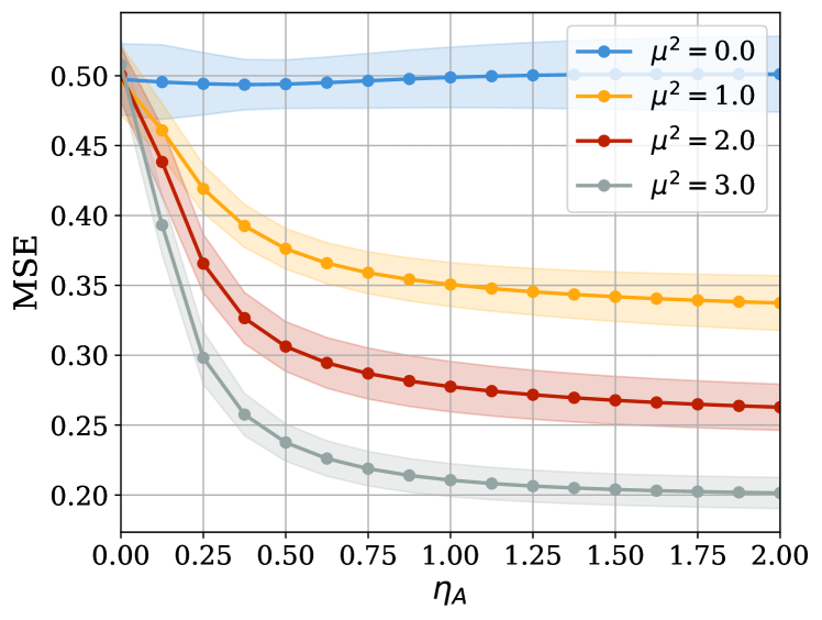
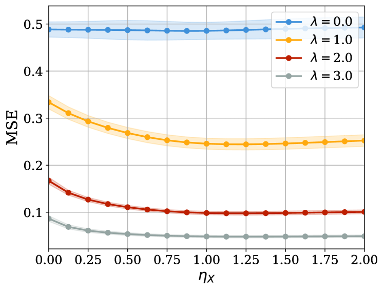
The idea is that although this leads to more noise terms, the signal strength of $\bm{yy}^{T}$ is increased more. Instead of a weighting of $\frac{\lambda}{N}\bm{yy}^{T}$, we now have $(\frac{\lambda}{N}+\eta_{A}\frac{\mu^{2}F}{N})\bm{yy}^{T}$. The new MSE also concentrates on a value determined by $\eta_{A}$. So, numerically, as shown in Figure 14, for any $\mu,|\lambda|>0$ we can always find values of $\eta_{A}$ such that the MSE is decreased. For denoising $\bm{X}$ we do

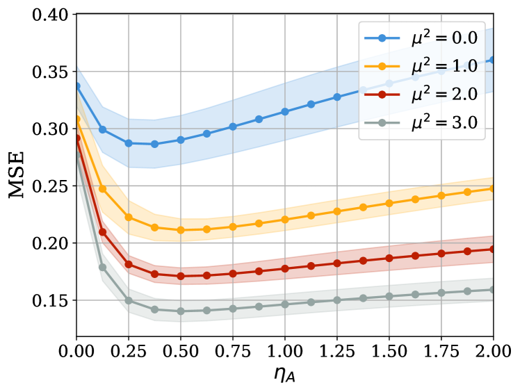
$$\bm{X}_{\text{den}}=\bm{X}+\eta_{X}\bm{A}\bm{X}$$ (9)

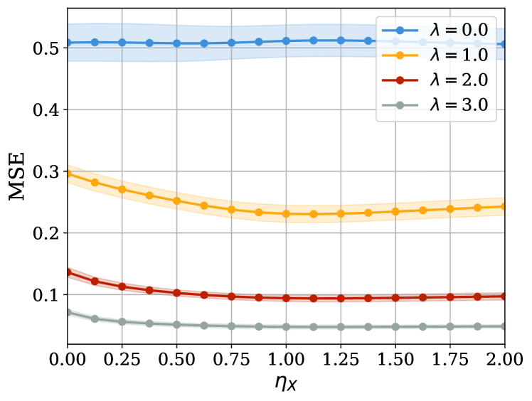
and show in Figure 15 with the same argumentation as for $\bm{A}$ that an $\eta_{X}$ exists so that the MSE is reduced. Proof of both cases has yet to be provided and will be the subject of future work.

References

- Abbe [2018] E. Abbe. Community detection and stochastic block models: Recent developments. Journal of Machine Learning Research, 18(177):1–86, 2018. URL http://jmlr.org/papers/v18/16-480.html.
- Alon and Yahav [2021] U. Alon and E. Yahav. On the bottleneck of graph neural networks and its practical implications. In International Conference on Learning Representations, 2021. URL https://openreview.net/forum?id=i80OPhOCVH2.
- Banerjee et al. [2022] P. K. Banerjee, K. Karhadkar, Y. G. Wang, U. Alon, and G. Montúfar. Oversquashing in gnns through the lens of information contraction and graph expansion. In 2022 58th Annual Allerton Conference on Communication, Control, and Computing (Allerton), page 1–8. IEEE Press, 2022. doi: 10.1109/Allerton49937.2022.9929363. URL https://doi.org/10.1109/Allerton49937.2022.9929363.
- Battaglia et al. [2018] P. W. Battaglia, J. B. Hamrick, V. Bapst, A. Sanchez-Gonzalez, V. Zambaldi, M. Malinowski, A. Tacchetti, D. Raposo, A. Santoro, R. Faulkner, C. Gulcehre, F. Song, A. Ballard, J. Gilmer, G. Dahl, A. Vaswani, K. Allen, C. Nash, V. Langston, C. Dyer, N. Heess, D. Wierstra, P. Kohli, M. Botvinick, O. Vinyals, Y. Li, and R. Pascanu. Relational inductive biases, deep learning, and graph networks, 2018.
- Black et al. [2023] M. Black, Z. Wan, A. Nayyeri, and Y. Wang. Understanding oversquashing in GNNs through the lens of effective resistance. In A. Krause, E. Brunskill, K. Cho, B. Engelhardt, S. Sabato, and J. Scarlett, editors, Proceedings of the 40th International Conference on Machine Learning, volume 202 of Proceedings of Machine Learning Research, pages 2528–2547. PMLR, 7 2023. URL https://proceedings.mlr.press/v202/black23a.html.
- Chen et al. [2020a] D. Chen, Y. Lin, W. Li, P. Li, J. Zhou, and X. Sun. Measuring and relieving the over-smoothing problem for graph neural networks from the topological view. Proceedings of the AAAI Conference on Artificial Intelligence, 34(04):3438–3445, 4 2020a. doi: 10.1609/aaai.v34i04.5747. URL https://ojs.aaai.org/index.php/AAAI/article/view/5747.
- Chen et al. [2020b] Y. Chen, L. Wu, and M. Zaki. Iterative deep graph learning for graph neural networks: Better and robust node embeddings. In H. Larochelle, M. Ranzato, R. Hadsell, M. Balcan, and H. Lin, editors, Advances in Neural Information Processing Systems, volume 33, pages 19314–19326. Curran Associates, Inc., 2020b. URL https://proceedings.neurips.cc/paper_files/paper/2020/file/e05c7ba4e087beea9410929698dc41a6-Paper.pdf.
- Chien et al. [2021] E. Chien, J. Peng, P. Li, and O. Milenkovic. Adaptive universal generalized pagerank graph neural network. In International Conference on Learning Representations, 2021. URL https://openreview.net/forum?id=n6jl7fLxrP.
- Deac et al. [2022] A. Deac, M. Lackenby, and P. Veličković. Expander graph propagation. In NeurIPS 2022 Workshop on Symmetry and Geometry in Neural Representations, 2022. URL https://openreview.net/forum?id=6cthqh2qhCT.
- Deshpande et al. [2018] Y. Deshpande, S. Sen, A. Montanari, and E. Mossel. Contextual stochastic block models. Advances in Neural Information Processing Systems, 31, 2018.
- Dong and Kluger [2023] M. Dong and Y. Kluger. Towards understanding and reducing graph structural noise for GNNs. In A. Krause, E. Brunskill, K. Cho, B. Engelhardt, S. Sabato, and J. Scarlett, editors, Proceedings of the 40th International Conference on Machine Learning, volume 202 of Proceedings of Machine Learning Research, pages 8202–8226. PMLR, 07 2023. URL https://proceedings.mlr.press/v202/dong23a.html.
- Duranthon and Zdeborová [2023] O. Duranthon and L. Zdeborová. Optimal inference in contextual stochastic block models, 2023.
- Erdös and Rényi [1959] P. Erdös and A. Rényi. On random graphs i. Publicationes Mathematicae Debrecen, 6:290–297, 1959.
- Fesser and Weber [2023] L. Fesser and M. Weber. Mitigating over-smoothing and over-squashing using augmentations of forman-ricci curvature. In The Second Learning on Graphs Conference, 2023. URL https://openreview.net/forum?id=bKTkZMRtfC.
- Fey and Lenssen [2019] M. Fey and J. E. Lenssen. Fast graph representation learning with PyTorch Geometric. In ICLR Workshop on Representation Learning on Graphs and Manifolds, 2019.
- Gasteiger et al. [2019] J. Gasteiger, S. Weiß enberger, and S. Günnemann. Diffusion improves graph learning. In H. Wallach, H. Larochelle, A. Beygelzimer, F. d'Alché-Buc, E. Fox, and R. Garnett, editors, Advances in Neural Information Processing Systems, volume 32. Curran Associates, Inc., 2019. URL https://proceedings.neurips.cc/paper_files/paper/2019/file/23c894276a2c5a16470e6a31f4618d73-Paper.pdf.
- Gilmer et al. [2017] J. Gilmer, S. S. Schoenholz, P. F. Riley, O. Vinyals, and G. E. Dahl. Neural message passing for quantum chemistry. In Proceedings of the 34th International Conference on Machine Learning - Volume 70, ICML’17, page 1263–1272. JMLR.org, 2017.
- Gligorijevic et al. [2019] V. Gligorijevic, P. Renfrew, T. Kosciolek, J. Koehler, K. Cho, T. Vatanen, D. Berenberg, B. Taylor, I. Fisk, R. Xavier, R. Knight, and R. Bonneau. Structure-based function prediction using graph convolutional networks, 10 2019.
- Karhadkar et al. [2023] K. Karhadkar, P. K. Banerjee, and G. Montufar. FoSR: First-order spectral rewiring for addressing oversquashing in GNNs. In The Eleventh International Conference on Learning Representations, 2023. URL https://openreview.net/forum?id=3YjQfCLdrzz.
- Kipf and Welling [2017] T. N. Kipf and M. Welling. Semi-supervised classification with graph convolutional networks. In International Conference on Learning Representations, 2017. URL https://openreview.net/forum?id=SJU4ayYgl.
- Li et al. [2019] P. Li, I. Chien, and O. Milenkovic. Optimizing generalized pagerank methods for seed-expansion community detection. In Advances in Neural Information Processing Systems, volume 32. Curran Associates, Inc., 2019. URL https://proceedings.neurips.cc/paper_files/paper/2019/file/9ac1382fd8fc4b631594aa135d16ad75-Paper.pdf.
- Linkerhägner et al. [2023] J. Linkerhägner, N. Freymuth, P. M. Scheikl, F. Mathis-Ullrich, and G. Neumann. Grounding graph network simulators using physical sensor observations. In The Eleventh International Conference on Learning Representations, 2023. URL https://openreview.net/forum?id=jsZsEd8VEY.
- Liu et al. [2022] S. Liu, R. Ying, H. Dong, L. Lin, J. Chen, and D. Wu. How powerful is implicit denoising in graph neural networks, 2022.
- Lv et al. [2023] S. Lv, G. Wen, S. Liu, L. Wei, and M. Li. Robust graph structure learning with the alignment of features and adjacency matrix, 2023.
- Ma et al. [2021] Y. Ma, X. Liu, T. Zhao, Y. Liu, J. Tang, and N. Shah. A unified view on graph neural networks as graph signal denoising. In Proceedings of the 30th ACM International Conference on Information & Knowledge Management, CIKM ’21, page 1202–1211, New York, NY, USA, 2021. ISBN 9781450384469. doi: 10.1145/3459637.3482225.
- Mandal et al. [2022] R. Mandal, C. Casert, and P. Sollich. Robust prediction of force chains in jammed solids using graph neural networks. Nature Communications, 13:4424, 07 2022. doi: 10.1038/s41467-022-31732-3.
- McAuley et al. [2015] J. McAuley, C. Targett, Q. Shi, and A. van den Hengel. Image-based recommendations on styles and substitutes. In Proceedings of the 38th International ACM SIGIR Conference on Research and Development in Information Retrieval, SIGIR ’15, page 43–52, New York, NY, USA, 2015. Association for Computing Machinery. ISBN 9781450336215. doi: 10.1145/2766462.2767755. URL https://doi.org/10.1145/2766462.2767755.
- McPherson et al. [2001] M. McPherson, L. Smith-Lovin, and J. M. Cook. Birds of a feather: Homophily in social networks. Annual Review of Sociology, 27:415–444, 2001. ISSN 03600572, 15452115. URL http://www.jstor.org/stable/2678628.
- Ng et al. [2001] A. Ng, M. Jordan, and Y. Weiss. On spectral clustering: Analysis and an algorithm. In T. Dietterich, S. Becker, and Z. Ghahramani, editors, Advances in Neural Information Processing Systems, volume 14. MIT Press, 2001. URL https://proceedings.neurips.cc/paper_files/paper/2001/file/801272ee79cfde7fa5960571fee36b9b-Paper.pdf.
- Nguyen et al. [2023] K. Nguyen, N. M. Hieu, V. D. Nguyen, N. Ho, S. Osher, and T. M. Nguyen. Revisiting over-smoothing and over-squashing using ollivier-ricci curvature. In A. Krause, E. Brunskill, K. Cho, B. Engelhardt, S. Sabato, and J. Scarlett, editors, Proceedings of the 40th International Conference on Machine Learning, volume 202 of Proceedings of Machine Learning Research, pages 25956–25979. PMLR, 7 2023. URL https://proceedings.mlr.press/v202/nguyen23c.html.
- Pan et al. [2022] L. Pan, C. Shi, and I. Dokmanić. Neural link prediction with walk pooling. In International Conference on Learning Representations, 2022. URL https://openreview.net/forum?id=CCu6RcUMwK0.
- Pei et al. [2020] H. Pei, B. Wei, K. C.-C. Chang, Y. Lei, and B. Yang. Geom-gcn: Geometric graph convolutional networks. In International Conference on Learning Representations, 2020. URL https://openreview.net/forum?id=S1e2agrFvS.
- Rozemberczki et al. [2021] B. Rozemberczki, C. Allen, and R. Sarkar. Multi-Scale attributed node embedding. Journal of Complex Networks, 9(2):cnab014, 05 2021. ISSN 2051-1329. doi: 10.1093/comnet/cnab014. URL https://doi.org/10.1093/comnet/cnab014.
- Sen et al. [2008] P. Sen, G. Namata, M. Bilgic, L. Getoor, B. Galligher, and T. Eliassi-Rad. Collective classification in network data. AI Magazine, 29(3):93, 9 2008. doi: 10.1609/aimag.v29i3.2157. URL https://ojs.aaai.org/aimagazine/index.php/aimagazine/article/view/2157.
- Shi et al. [2024] C. Shi, L. Pan, H. Hu, and I. Dokmanić. Homophily modulates double descent generalization in graph convolution networks. Proceedings of the National Academy of Sciences, 121(8):e2309504121, 2024. doi: 10.1073/pnas.2309504121. URL https://www.pnas.org/doi/abs/10.1073/pnas.2309504121.
- Shi and Malik [2000] J. Shi and J. Malik. Normalized cuts and image segmentation. IEEE Transactions on Pattern Analysis and Machine Intelligence, 22(8):888–905, 2000. doi: 10.1109/34.868688.
- Tang et al. [2009] J. Tang, J. Sun, C. Wang, and Z. Yang. Social influence analysis in large-scale networks. In Proceedings of the 15th ACM SIGKDD International Conference on Knowledge Discovery and Data Mining, KDD ’09, page 807–816, New York, NY, USA, 2009. Association for Computing Machinery. ISBN 9781605584959. doi: 10.1145/1557019.1557108. URL https://doi.org/10.1145/1557019.1557108.
- Topping et al. [2022] J. Topping, F. D. Giovanni, B. P. Chamberlain, X. Dong, and M. M. Bronstein. Understanding over-squashing and bottlenecks on graphs via curvature. In International Conference on Learning Representations, 2022. URL https://openreview.net/forum?id=7UmjRGzp-A.
- Wang et al. [2024] J. Wang, J. Guo, Y. Sun, J. Gao, S. Wang, Y. Yang, and B. Yin. Dgnn: Decoupled graph neural networks with structural consistency between attribute and graph embedding representations, 2024.
- Wu et al. [2023] X. Wu, Z. Chen, W. W. Wang, and A. Jadbabaie. A non-asymptotic analysis of oversmoothing in graph neural networks. In The Eleventh International Conference on Learning Representations, 2023. URL https://openreview.net/forum?id=CJd-BtnwtXq.
- Zhou et al. [2020] J. Zhou, G. Cui, S. Hu, Z. Zhang, C. Yang, Z. Liu, L. Wang, C. Li, and M. Sun. Graph neural networks: A review of methods and applications. AI Open, 1:57–81, 2020. ISSN 2666-6510. doi: https://doi.org/10.1016/j.aiopen.2021.01.001.
- Zhu et al. [2020] J. Zhu, Y. Yan, L. Zhao, M. Heimann, L. Akoglu, and D. Koutra. Beyond homophily in graph neural networks: Current limitations and effective designs. In H. Larochelle, M. Ranzato, R. Hadsell, M. Balcan, and H. Lin, editors, Advances in Neural Information Processing Systems, volume 33, pages 7793–7804. Curran Associates, Inc., 2020. URL https://proceedings.neurips.cc/paper_files/paper/2020/file/58ae23d878a47004366189884c2f8440-Paper.pdf.
- Zhu et al. [2022] Y. Zhu, W. Xu, J. Zhang, Y. Du, J. Zhang, Q. Liu, C. Yang, and S. Wu. A survey on graph structure learning: Progress and opportunities, 2022.
- Zhu et al. [2024] Y. Zhu, R. Amor, Y. Chen, Z. Deng, L. Feng, and M. Witbrock. Robust node classification on graph data with graph and label noise. Proceedings of the AAAI Conference on Artificial Intelligence, 2024.