|
|
|
|
(3) |
|
|
|
|
|
|
|
|
|
|
|
|
|
|
|
|
|
|
|
|
|
|
|
|
where and and have been implicitly defined. Indeed,
arises from the fact that and can be written in
terms of and Also,
|
|
|
(4) |
so that
|
|
|
|
|
|
|
|
|
|
|
|
|
|
|
|
|
|
|
|
where and are defined below in (5) and (6). In fact, arises from the fact that and can be written in terms of Furthermore,
|
|
|
and
|
|
|
|
|
|
|
|
In general,
|
|
|
|
|
|
|
|
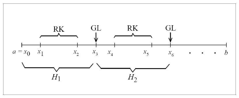
In the above, and are appropriate coefficients (defined below), and is the
total number of subintervals into which has been subdivided. We
list below some relevant terms in detail.
|
|
|
|
(5) |
|
|
|
|
|
|
|
|
|
|
|
|
(6) |
|
|
|
|
|
|
|
|
In general,
|
|
|
For completeness, we could include a term of the form
|
|
|
in the expression for above, but we assume that so that such a term is not necessary here.
|
|
|
|
|
|
|
|
|
|
|
|
|
|
|
|
|
|
|
|
|
|
|
|
Using the above expressions, we have, in terms of the local errors
|
|
|
where
|
|
|
|
|
|
|
|
|
|
|
|
|
|
|
|
|
|
|
|
|
|
|
|
(7) |
|
|
|
|
|
|
|
|
|
|
|
|
|
|
|
|
|
|
|
|
|
|
|
|
The global error at the RK nodes is understood with reference to section
2.3, and equations (3) and (4).