pyBregMan: A Python library for Bregman Manifolds††thanks: https://franknielsen.github.io/pyBregMan/
Abstract
A Bregman manifold is a synonym for a dually flat space in information geometry which admits as a canonical divergence a Bregman divergence. Bregman manifolds are induced by smooth strictly convex functions like the cumulant or partition functions of regular exponential families, the negative entropy of mixture families, or the characteristic functions of regular cones just to list a few such convex Bregman generators. We describe the design of pyBregMan, a library which implements generic operations on Bregman manifolds and instantiate several common Bregman manifolds used in information sciences. At the core of the library is the notion of Legendre-Fenchel duality inducing a canonical pair of dual potential functions and dual Bregman divergences. The library also implements the Fisher-Rao manifolds of categorical/multinomial distributions and multivariate normal distributions. To demonstrate the use of the pyBregMan kernel manipulating those Bregman and Fisher-Rao manifolds, the library also provides several core algorithms for various applications in statistics, machine learning, information fusion, and so on.
Key words: Dually flat space; Hessian manifold; Fisher-Rao manifold; geodesics; Legendre-Fenchel transform; duality; auto-differentiation; clustering; Jensen divergence; Bregman divergence; Jensen-Shannon centroid; Chernoff information; multivariate normal manifolds: categorical manifolds
1 Getting started with pyBregMan
Let us build, step-by-step, a simple example to demonstrate usage of the pyBregMan library
(Python library for Bregman Manifolds):
① we create the Bregman and Fisher-Rao manifold structures for the
family of bivariate normal distributions (namely, an exponential family
manifold and a Fisher-Rao manifold);
② we calculate the Kullback-Leibler
divergence between two bivariate normal distributions;
③ we compute
the left-sided Kullback-Leibler, right-sided Kullback-Leibler, Bhattacharyya
and Fisher-Rao centroids [33, 29] (Riemannian geodesic
midpoint); and
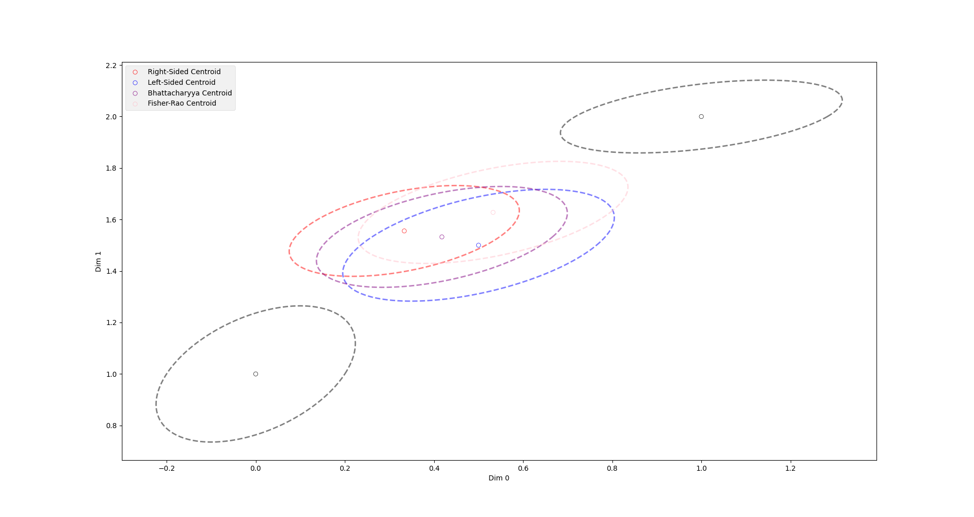
④ we visualize those bivariate normal centroids
(Figure 1).
The basic usage of pyBregMan consists of defining a specific Bregman manifold, defining points on said manifold, and then defining additional geometric objects on the manifold.
To install the library via pip3, execute the command:
pip3 install pyBregMan
Alternatively, the library can be installed from GitHub as follows:
git clone https://github.com/alexandersoen/pyBregMan.git cd pyBregMan pip3 install .
In the following example, we first define a the manifold of bivariate normal distributions. The following code illustrates the construction of a bivariate Gaussian Bregman manifold (see §2 for a quick review of the theory of Bregman manifolds).
Here the manifold bivariate normal distributions is defined via GaussianManifold. In pyBregMan, we provide a variety of different manifolds used in information sciences. These can be found under the bregman.application submodule. To define data on the manifold, one needs to use the Point primitive. Here data is annotated with a coordinate type LAMBDA_COORDS (see [30]), which for Gaussian distributions corresponds to the typical mean and covariance matrix of Gaussians represented as a vector.
Simple calculations for (exponential family) distributions can be directly called from the manifold. For instance, the Kullback-Leibler divergence between the points can be called as follows:
Additional geometric objects and calculations can be called by external submodules. For instance, various barycenter (weighted centroid) calculations can be found in bregman.barycenter. Additionally, manifold specific geometric objects can be found in their specific submodule, see for instance FisherRaoKobayashiGeodesic. Here we are utilizing the fact that the Fisher-Rao centroid between two points is the midpoint of the corresponding Fisher-Rao geodesic [10, 24].
Finally, we can visualize the objects on the manifold in matplotlib [9] via using the ‘MatplotlibVisualizer‘ class and specifying the objects to plot. One can also register additional callback functions to enhance the visualization. Here we utilize a Tissot-style visualization of the covariance matrices whilst plotting the mean vector. The final visualization is shown in Figure 1. Notice that the plot_object function accepts typical matplotlib arguments.
2 A short introduction to Bregman and Fisher-Rao manifolds
We first briefly review the concepts of Bregman manifolds and its relationship with Fisher-Rao manifolds in §2.1. Then we explain the goals of the pyBregMan library in §2.4. Let us mention the GeomStats Python library which includes an information geometry package [11] implementing Fisher-Rao manifolds, and the Manifolds.jl Julia package [2] among other public libraries.
2.1 Bregman manifolds: A quick review
Let be a strictly convex and differentiable real-valued convex function defined over a topologically open domain . The Bregman divergence [6] between and is a measure of dissimilarity defined by the following formula:
where is the Euclidean inner product called dot product or scalar product.
When the Bregman generator inducing the Bregman divergence is and of Legendre-type [40], a Bregman divergence induces a dually flat space in information geometry [1] with a single global chart .
The torsion-free affine connections and induced respectively by and its convex conjugate111The convex conjugate of a Legendre-type function is of Legendre-type, and the Legendre-Fenchel transform is involutive. We have two gradient maps: and which are reciprocal to each other (i.e., ), and the convex conjugate is given by the Legendre function . are flat and coupled to the metric tensor . The metric is of type Hessian and can be expressed either in the -coordinate system or the dual -coordinate system equivalently by
Dually flat spaces are special cases of Hessian manifolds [41] which possibly admit several charts and local dual potential functions and related by the Legendre-Fenchel transformation.
We term Hessian manifolds with single charts or dually flat spaces Bregman manifolds because conversely, a single chart manifold with a dual structure admits a pair of canonical potential functions and such that its coordinate-free dually flat divergence between points and of (with and ) can be expressed equivalently as:
where is the Fenchel-Young divergence [4, 22]:
See [20] for more details on Bregman manifolds.
Notice that the potential functions and reconstructed from are not unique [1] but defined up to affine terms. That is, we may consider equivalently the primal potential function:
for , and , and its corresponding convex conjugate to build the same information-geometric structure . This property has been called affine Legendre equivalence in [14]. See §4 of [23] for more details.
Bregman manifolds can be constructed from convex functions arising from statistical models. For example,
-
•
When is the cumulant function of an exponential family [1], we get a Bregman manifold with Bregman divergence corresponding to the reverse Kullback-Leibler divergence [27]. When choosing the partition function instead of (a log-convex function hence convex), the Bregman divergence amounts to the Kullback-Leibler divergence between unnormalized densities [28].
- •
-
•
All statistical models parameterized by either one or two parameters can yield Bregman manifolds because the 2D Fisher-Rao metrics are Hessian. See for example the case of univariate elliptical distributions [13].
2.2 Fisher-Rao manifolds
A Fisher-Rao manifold [39] is a Riemannian manifold induced by the Fisher information metric of a statistical model which yields a geodesic distance called Rao’s distance [7]. When the Fisher information metric is Hessian and defined according to a single chart (i.e., there exists a coordinate system and a potential function such that ), the Fisher-Rao manifold can also be considered as a Bregman manifold.
For example, the Fisher-Rao manifold of the statistical model of univariate Gaussian distributions is Hessian since parameterized by a 2D parameter. This manifolds is also a Bregman manifold. Figure 2 for illustrates the Fisher-Rao geodesic (purple), -geodesic (called -geodesic in blue induced by the cumulant function ) and the -geodesic (called -geodesic in red) used for the logo of pyBregMan. The -geodesics correspond to the -geometry and the Fisher-Rao geodesic to the self-dual -geometry, see [1].

2.3 Divergence-based information geometry
Given a smooth divergence , Eguchi [8] proposed a method to induce a divergence-based manifold, i.e., a dualistic structure related to the forward divergence and reverse divergence . In particular, when is a Bregman divergence, the divergence-based manifold amounts to a Bregman manifold.
When is Zhang -divergence [42] (also called Burbea-Rao divergence in [29]):
the divergence-based manifold induced by is a -Hessian manifold [43] which corresponds to the -geometry [1] extending the dual Bregman manifolds which are obtained in the limit cases and :
By continuity, we let and . Figure 3 shows how structures and divergences relate to each others.
The -Hessian manifold correspond to the Fisher-Rao manifold when the Fisher metric is Hessian, and the statistical divergence corresponding to induced by the cumulant function of an exponential family is the Bhattacharyya distance [29].

2.4 Purposes of the library
The three main goals of the pyBregMan library are
-
1.
To provide a geometric kernel to implement, visualize, and export figures of main concepts of Bregman manifolds in 2D and 3D (e.g., dual coordinates which are -affine coordinate systems, reciprocal basis, connection-based geodesics, metric-compatible parallel transport, Bregman balls, Bregman projections, etc.);
-
2.
To provide APIs for handling the Fisher-Rao manifolds and the dualistic structure (-geometry) in information geometry of statistical models with Fisher information of Hessian type;
-
3.
To use the APIs to demonstrate use cases of information geometry on exponential and mixture families: For example, to compute the Chernoff information [21], to approximate the matrix geometric mean [15], or to compute the discrete Jensen-Shannon centroid [18], etc. That is, to ease the programming of information geometry in action in various fields of information sciences.
In particular, we shall consider the following Bregman manifolds:
3 Structure of the library
In the following section, we outline the structure of the pyBregMan library. Additionally, we highlight connections between specific implementation details and API design which corresponds to the concepts of Bregman manifolds, i.e., Section 2.1. We first highlight core primitives of the library, clarifying how manifold objects and data interact within pyBregMan. We then outline additional geometric objects which are currently included in the library. Defined application manifolds which can be readily used are presented. Finally, we present the visualization pipeline.
3.1 Primitives of the Library
Various primitives of pyBregMan are found in the bregman.base and bregman.manifold submodules. We will examine the Coords type and the BregmanManifold abstract class.
3.1.1 Coordinates and Points
From the former, an important aspect of the library is how the Coords class annotates different geometric objects, which inherit from CoordObject. For instance, Point provides a coordinate type annotation for data to be used in our manifolds. All Bregman manifolds are equipped with THETA_COORDS (-coordinate system) and ETA_COORDS (-coordinate system) which are instances of coordinates Coords. Additional instances of Coords can be defined, for instance LAMBDA_COORDS (ordinary parameters) for Gaussian distributions, see Section 1. A subset of coordinates are defined by DualCoords, which provide an enum type restricted to only -and -coordinate systems. This provides restriction of the pyBregMan API for geometric objects which are only defined w.r.t. -and -coordinate systems.
Notice that in the discussion of the coordinate system typing of the library, no specific manifold has been specified. Indeed, currently data defined by Point can be freely switched between different manifolds under the assumption that the dimension (shape of the data) and constraints (e.g., ensuring positive semi-definiteness of Gaussian covariances) of the data is valid in each manifold.
3.1.2 Bregman Manifolds
The bregman.manifold submodule provides the main components of all manifold classes defined in the library. In particular, all manifold objects in pyBregMan implement from the abstract class BregmanManifold in bregman.manifold.manifold. The dependency graph of BregmanManifold is shown in Figure 4. A BregmanManifold must define two Bregman Generators and define the dimension of the generators’ inputs. The two generators consist of a theta_generator and a eta_generator . pyBregMan assumes that the defined generator classes are dual. An eta_generator is optional in its definition and can be set to None; however, this would greatly limit the functionality of the manifold.
The prescribed Generator class requires / to be twice differentiable, with their corresponding derivatives defined, see its corresponding methods in Figure 4. For quick development and easier usage, we provide AutoDiffGenerator in bregman.manifold.generator, which uses the autograd library to automatically calculate the required first and second derivatives via auto-differentiation. As such, by using AutoDiffGenerator, a user only needs to define with gradient and Hessian automatically defined. We do note that for numeric precision, one may still want to define the derivatives explicitly.
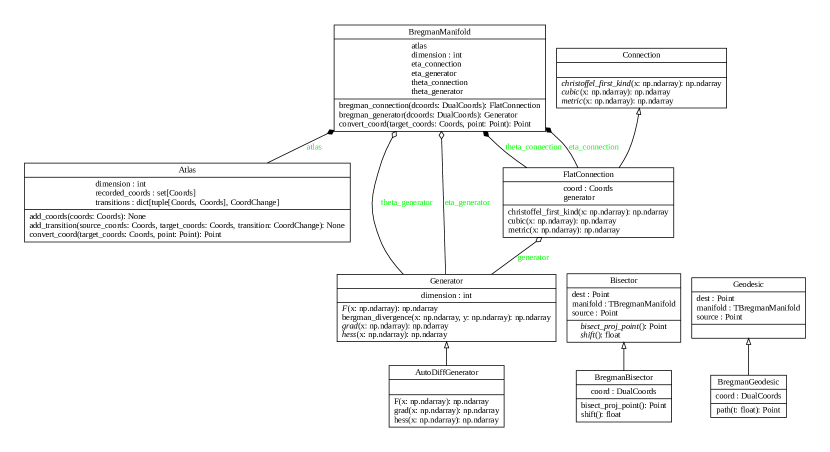
The FlatConnection composition in BregmanManifold simply defines the torsion-free affine connections induced by the input Generators (utilizes auto-differentiation to calculate the metric).
Finally, the Atlas composition in BregmanManifold is a class which provides management of the different coordinate systems specified by Coords. In particular, it allows instances of Coords and coordinate changes to be registered in the BregmanManifold. This allows coordinate dependent geometric operations to be freely utilized on data which may potentially have different coordinates. We show instances of this convenience in Section 3.2. It should be noted to allow coordinate changes between all registered coordinate systems, all combinations of coordinate changes must be defined. The conversion between -and -coordinates are automatically defined via and , respectively.
3.1.3 Geodesics and Bisectors
Two additional geometric objects that are defined in the bregman.manifold submodule are the Geodesic and Bisector objects [5]. For the latter, Bisector is currently only for visualization, see Section 4.3. Geodesic defines an abstract object, which when implemented provides a curve object which returns points when given a value , mapping from source () to destination (). In bregman.manifold.geodesic, a concrete implementation of BregmanGeodesic is defined. This allows a -or -geodesic to be defined for a specified manifold. Its implementation is shown in the following.
In addition the source and dest data Points, it takes in a BregmanManifold and a DualCoord. This allows the source and destination point of the geodesic to be converted into the specified dually flat coordinate (as per dcoords: DualCoords) to define the geodesic via linear interpolation.
3.2 Additional Geometric Objects
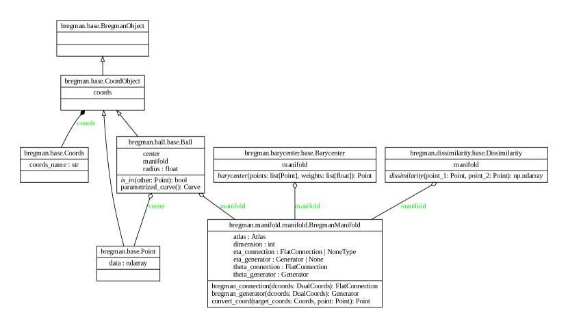
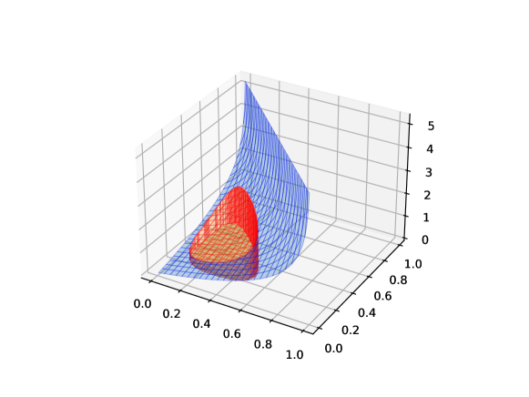
In the following, we provide a brief description the additional geometric objects provided by pyBregMan. We only discuss their abstract classes and leave example usages to Section 4. The geometric objects can be depicted in Figure 5.
-
•
bregman.ball.base.Ball: The Ball class allows objects such as Bregman balls to be defined in the library. It is defined from a ball center and a radius. Currently, the functionality of the class is limited to checking whether or not a point is inside the ball via the is_in method. Unlike the other geometric objects discussed in this subsection, Ball is a CoordObject. This means that Ball must have a “natural” coordinate system attributed to its. Bregman balls are basic geometric objects used in proximity query data structures [34, 35]. The smallest enclosing Bregmall ball of a set of points has been studied in [32, 36]. Bregman balls can be considered as intersections of hyperplanes with the graph of the potential function [5], see Figure 6.
-
•
bregman.barycenter.base.Barycenter: The Barycenter class provides an interface for different barycenter algorithms to be defined. In particular, for a particular manifold, it implements a method barycenter which “aggregates” a list of points list[Point] and a list of weights list[float] (of the same length). Examples of concrete implementations of Barycenter can be found in Section 1.
-
•
bregman.dissimilarity.base.Dissimilarity: The Dissimilarity class provides an interface for the definition of dissimilarity functions in the library. These are the class of function which accepts two points and calculates a dissimilarity measure. An example of a concrete implementation of Dissimilarity is the BregmanDivergence. In information geometry, a smooth dissimilarity is called a divergence and interpreted as a function on the product manifold: a yoke [3] or contrast function [12].
3.3 Application Manifolds
We provide a variety of application manifolds in pyBregMan. These manifolds are concrete implementations of the BregmanManifold. In particular, they all inherit from the ApplicationManifold class in the submodule bregman.application.application. Implementing ApplicationManifold has two additional requirements over BregmanManifold. First, a -coordinate system needs to be defined. This is typically a representation of points in the manifold which do not correspond to either the -or -coordinates. Secondly, a DisplayPoint needs to be defined. This is just a pretty-printing wrapper for a specific coordinate system.
The following presents a list of implemented application manifolds.
-
•
Distributions (statistical models):
-
–
Exponential Family
-
*
bregman.application.distribution.exponential_family
.gaussian.GaussianManifold -
*
bregman.application.distribution.exponential_family
.multinomial.MultinomialManifold -
*
bregman.application.distribution.exponential_family
.categorical.CategoricalManifold
-
*
-
–
Mixture
-
*
bregman.application.distribution.mixture
.discrete_mixture.DiscreteMixture -
*
bregman.application.distribution.mixture
.ef_mixture.EFMixtureManifold
-
*
-
–
-
•
bregman.application.psd.PSDManifold
In each submodule, additional subclasses of ApplicationManifold are defined and used. For instance, all DistributionManifolds require a mapping from Point to Distribution (from bregman.object.distribution).
In addition to the manifold defined, additional manifold specific geometric objects are sometimes defined. For instance, the GaussianManifold contains additional submodules which defines Gaussian specific dissimilarity measures and geodesics. Notably, we provide implementations of approximate Fisher-Rao distance and geodesics using Kobayashi’s approximation [10].
3.4 Visualization
pyBregMan provides a visualization submodule in bregman.visualizer. In particular, MatplotlibVisualizer in bregman.visualizer.matplotlib provides an implementation of a visualizer using the matploblib library [9]. The visualizer implements a plot function for every subtype of BregmanObject (defined in bregman.base). These are points Point, geodesics Geodesic, and bisectors Bisector. Additional VisualizerCallbacks can be defined if additional plotting functionality is desired. Also note that matplotlib specific arguments can also be used when using MatplotlibVisualizer, see Section 1.
4 Some examples of Hessian Fisher-Rao statistical models
In the following section, we present a series of visual vignettes to demonstrate different uses of pyBregMan. In particular, we consider the following examples:
- •
- •
-
•
Gaussian Distributions: Calculating the Chernoff point [21] which is useful in Bayesian hypothesis testing and in information fusion tasks.
4.1 Positive Semi-definite Matrices: Geometric Matrix Means
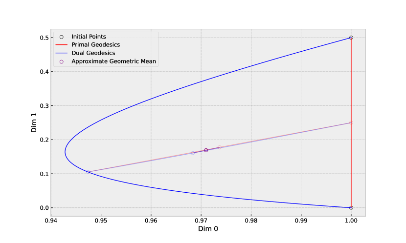
In the space of Positive Semi-definite (PSD) matrices, an iterative algorithm exists to obtain the mid-point of the Riemannian geodesic. In particular, it has been shown that by iteratively taking the arithmetic and harmonic mean between PSD matrices, and then setting those means as the new “initial” points, one will converge in a quadratic order to the geometric mean [16]. For PSD matrices, the geometric mean between matrices corresponds to the mid-point of the Riemannian geodesic; and the arithmetic mean and geometric mean correspond to the mid points of a primal-dual pair of geodesics.
Figure 7 demonstrates the inductive arithmetic-harmonic mean (AHM) algorithm for calculating the Riemannian geodesic mid-point. In particular, note the visualization of the primal and dual geodesic being plotted with their corresponding mid-points becoming the next starting points.
4.2 Categorical Distributions: Intensity Centroids
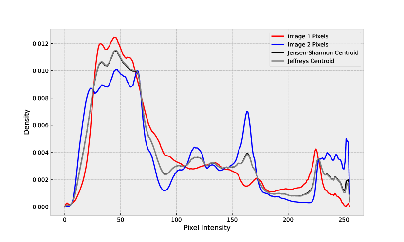
In the following example, we utilize pyBregMan to generate different types of centroid on the categorical distribution manifold. In particular, we consider the Jensen-Shannon centroid and its corresponding dual (Jeffreys Centroid) [18]. As we are working in the categorical manifold, we will utilize the convenient connection that the manifold of (discrete) mixture distributions is dual to the categorical manifold; and that the Jensen-Shannon divergences can be calculated as specific instances of the Burbea-Rao divergences on this mixture manifold [29].
To demonstrate this, we consider the task of computing centroid on histograms (categorical distributions) of images’ pixel intensity distributions. We specifically discretize the pixel intensity into 256 values corresponding to the average value over the 3 RGB color channels. The images that we consider in this example are those presented in Figure 8. The corresponding Jensen-Shannon and Jeffreys centroids are presented in Figure 9.


4.3 Gaussian Distributions: Chernoff Point / Information
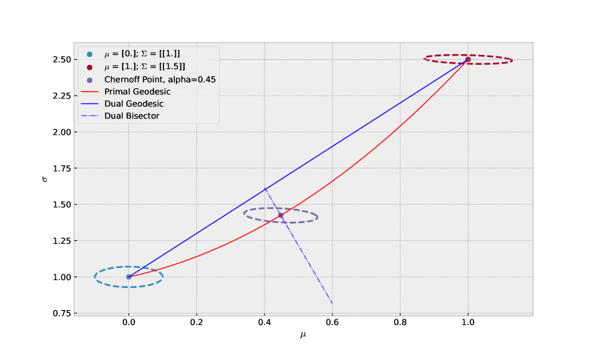
The Chernoff distance [21] or Chernoff information between two statistical distributions with densities and with respect to a base measure is defined by
It can be shown that the optimal value can be obtained by intersecting a primal Bregman geodesic with a dual Bregman bisector [21]. Figure 10 displays the so called Chernoff point [17] which can be calculated exactly on the univariate Gaussian manifold, and more generally approximated arbitrarily finely between any two densities of an exponential family.
5 Extending pyBregMan
In the following, we go through an example of extending pyBregMan by defining a new application manifold. In particular, we will go through the process of defining a minimal 2D Bregman manifold with primal generator specified as the extended negative Shannon entropy function. Overall, the process can be broken down into two steps:
-
•
The first is to define the pair of Bregman generators used to define the Bregman manifold.
-
•
The second is to define quantities and methods associated with the -coordinates, which is primarily used for displaying points on the manifold.
Finally, we will present an example of implementing new manifold specific geometric objects by defining a new Bregman ball object in this 2D manifold with parameterized equation.
5.1 Defining Generators using auto-differentiation
The first and primary task we will consider is defining the generators for the Bregman manifold. We will utilize AutoDiffGenerator from the bregman.manifold.generator submodule to define these Bregman generators. By utilizing auto-differentiation, we will only be required to define the generator functions itself and its derivatives will be automatically generated. Although these derivatives can be automatically calculated, we will still be required to implement the dual generator as there is no exact method for automatically generating it. As our primary generator, we utilize the extended negative Shannon entropy function [31]:
| (1) |
Through simple calculation, one can find that the dual generator:
| (2) |
Defining these generators in pyBregMan is straightforward:
One notable point in defining these generators in pyBregMan is that we must utilize ‘numpy‘ functions wrapped by the ‘autograd‘ library. Otherwise, the auto-differentiation procedure will not work.
5.2 Defining the Manifold
With these two generators defined for the Bregman manifold, all we need to do is define some quantities relating to a standard -parameterization. This acts as the “usual” parameterization that is used to define objects on the manifold. This can deviate from the canonical -or -parameterizations. In our case, we will simply specify the -parameterization to be equivalent to the -parameterization.
In terms of pyBregMan classes, we need to additionally define a corresponding DisplayPoint class. This is utilized for pretty printing the object and will correspond to the -parameterization of points. To change the default behaviour, one can override the convert_to_display method in ApplicationManifold. Nevertheless, the corresponding application manifold can be defined as:
Notice that the conversion between -and -parameterization are automatically defined through inheritance via the _theta_to_eta and _eta_to_theta methods. As such, we only needed to define the conversions w.r.t. the -coordinates.
The ApplicationManifold abstract class is generic and accepts a DisplayPoint type. We recommend specifying this to make it specific to the manifold’s display point type.
5.3 Defining Geometric Objects
Now utilizing the EKL2DManifold manifold we have just defined, we will define a Ball object specific to the manifold. We will utilize the closed form parameterization that is available for this specific Bregman manifold.
Here we are utilizing KL2DBregmanBallCurve which was not linked to a specific Ball implementation.
The Ball abstract class is generic and to make an subclass specific to a manifold type one can make the typing concrete. All geometric style objects follow pattern, e.g., Geodesic, Dissimilarity, etc.
Notice that extended KL sphere can be exactly rendered using the Lambert W function [19].
Notebook
A tutorial notebook entitled “Data Representations on the Bregman Manifold” demonstrating some aspects of the library is available at https://gram-blogposts.github.io/.
Acknowledgments
FN warmly thanks Richard Nock for many fruitful discussions on Bregman divergences and its use in machine learning. AS graciously thanks Ella Xi Wang for advice and assistance for module packaging and document generation in Python. AS would also like to thank Coco for providing excellent images for our code examples.
References
- [1] Shun-ichi Amari. Information Geometry and Its Applications. Applied Mathematical Sciences. Springer Japan, 2016.
- [2] Seth D Axen, Mateusz Baran, Ronny Bergmann, and Krzysztof Rzecki. Manifolds. jl: an extensible julia framework for data analysis on manifolds. ACM Transactions on Mathematical Software, 49(4):1–23, 2023.
- [3] Ole E Barndorff-Nielsen and Peter Edmund Jupp. Yokes and symplectic structures. Journal of statistical planning and inference, 63(2):133–146, 1997.
- [4] Mathieu Blondel, André FT Martins, and Vlad Niculae. Learning with Fenchel-Young losses. Journal of Machine Learning Research, 21(35):1–69, 2020.
- [5] Jean-Daniel Boissonnat, Frank Nielsen, and Richard Nock. Bregman Voronoi diagrams. Discrete & Computational Geometry, 44:281–307, 2010.
- [6] Lev M. Bregman. The relaxation method of finding the common point of convex sets and its application to the solution of problems in convex programming. USSR computational mathematics and mathematical physics, 7(3):200–217, 1967.
- [7] Jacob Burbea and C Radhakrishna Rao. Entropy differential metric, distance and divergence measures in probability spaces: A unified approach. Journal of Multivariate Analysis, 12(4):575–596, 1982.
- [8] Shinto Eguchi. Geometry of minimum contrast. Hiroshima Mathematical Journal, 22(3):631–647, 1992.
- [9] J. D. Hunter. Matplotlib: A 2d graphics environment. Computing in Science & Engineering, 9(3):90–95, 2007.
- [10] Shimpei Kobayashi. Geodesics of multivariate normal distributions and a Toda lattice type Lax pair. Physica Scripta, 98(11):115241, 2023.
- [11] Alice Le Brigant, Jules Deschamps, Antoine Collas, and Nina Miolane. Parametric information geometry with the package Geomstats. ACM Transactions on Mathematical Software, 49(4):1–26, 2023.
- [12] Takao Matumoto et al. Any statistical manifold has a contrast function—On the -functions taking the minimum at the diagonal of the product manifold. Hiroshima Math. J, 23(2):327–332, 1993.
- [13] Ann FS Mitchell. Statistical manifolds of univariate elliptic distributions. International Statistical Review/Revue Internationale de Statistique, pages 1–16, 1988.
- [14] Naomichi Nakajima and Toru Ohmoto. The dually flat structure for singular models. Information Geometry, 4(1):31–64, 2021.
- [15] Yoshimasa Nakamura. Algorithms associated with arithmetic, geometric and harmonic means and integrable systems. Journal of computational and applied mathematics, 131(1-2):161–174, 2001.
- [16] Yoshimasa Nakamura. Algorithms associated with arithmetic, geometric and harmonic means and integrable systems. Journal of computational and applied mathematics, 131(1-2):161–174, 2001.
- [17] Frank Nielsen. An information-geometric characterization of Chernoff information. IEEE Signal Processing Letters, 20(3):269–272, 2013.
- [18] Frank Nielsen. On a generalization of the Jensen–Shannon divergence and the Jensen–Shannon centroid. Entropy, 22(2):221, 2020.
- [19] Frank Nielsen. On geodesic triangles with right angles in a dually flat space. In Progress in Information Geometry: Theory and Applications, pages 153–190. Springer, 2021.
- [20] Frank Nielsen. The many faces of information geometry. Not. Am. Math. Soc, 69(1):36–45, 2022.
- [21] Frank Nielsen. Revisiting chernoff information with likelihood ratio exponential families. Entropy, 24(10):1400, 2022.
- [22] Frank Nielsen. Statistical divergences between densities of truncated exponential families with nested supports: Duo Bregman and duo Jensen divergences. Entropy, 24(3):421, 2022.
- [23] Frank Nielsen. Beyond scalar quasi-arithmetic means: Quasi-arithmetic averages and quasi-arithmetic mixtures in information geometry. arXiv preprint arXiv:2301.10980, 2023.
- [24] Frank Nielsen. Fisher-rao and pullback hilbert cone distances on the multivariate gaussian manifold with applications to simplification and quantization of mixtures. In Topological, Algebraic and Geometric Learning Workshops 2023, pages 488–504. PMLR, 2023.
- [25] Frank Nielsen. What is… an inductive mean? Notices of the American Mathematical Society, 70(11), 2023.
- [26] Frank Nielsen. Approximation and bounding techniques for the Fisher-Rao distances. arXiv preprint arXiv:2403.10089, 2024.
- [27] Frank Nielsen. Divergences induced by the cumulant and partition functions of exponential families and their deformations induced by comparative convexity. Entropy, 26(3):193, 2024.
- [28] Frank Nielsen. Divergences induced by the cumulant and partition functions of exponential families and their deformations induced by comparative convexity. Entropy, 26(3):193, 2024.
- [29] Frank Nielsen and Sylvain Boltz. The Burbea-Rao and Bhattacharyya centroids. IEEE Transactions on Information Theory, 57(8):5455–5466, 2011.
- [30] Frank Nielsen and Vincent Garcia. Statistical exponential families: A digest with flash cards. arXiv preprint arXiv:0911.4863, 2009.
- [31] Frank Nielsen and Gaëtan Hadjeres. Monte Carlo information-geometric structures. Geometric Structures of Information, pages 69–103, 2019.
- [32] Frank Nielsen and Richard Nock. On the smallest enclosing information disk. Information Processing Letters, 105(3):93–97, 2008.
- [33] Frank Nielsen and Richard Nock. Sided and symmetrized Bregman centroids. IEEE transactions on Information Theory, 55(6):2882–2904, 2009.
- [34] Frank Nielsen, Paolo Piro, and Michel Barlaud. Bregman vantage point trees for efficient nearest neighbor queries. In IEEE International Conference on Multimedia and Expo, pages 878–881. IEEE, 2009.
- [35] Frank Nielsen, Paolo Piro, and Michel Barlaud. Tailored Bregman ball trees for effective nearest neighbors. In Proceedings of the 25th European Workshop on Computational Geometry (EuroCG), pages 29–32, 2009.
- [36] Richard Nock and Frank Nielsen. Fitting the smallest enclosing Bregman ball. In European Conference on Machine Learning, pages 649–656. Springer, 2005.
- [37] Atsumi Ohara, Hideyuki Ishi, and Takashi Tsuchiya. Doubly autoparallel structure and curvature integrals: Applications to iteration complexity for solving convex programs. Information Geometry, 7(Suppl 1):555–586, 2024.
- [38] Atsumi Ohara, Nobuhide Suda, and Shun-ichi Amari. Dualistic differential geometry of positive definite matrices and its applications to related problems. Linear Algebra and its Applications, 247:31–53, 1996.
- [39] Calyampudi Radhakrishna Rao. Information and the accuracy attainable in the estimation of statistical parameters. Bulletin of the Calcutta Mathematical Society, 37(3):81–91, 1945.
- [40] Ralph Tyrrell Rockafellar. Conjugates and Legendre transforms of convex functions. Canadian Journal of Mathematics, 19:200–205, 1967.
- [41] Hirohiko Shima. The geometry of Hessian structures. World Scientific, 2007.
- [42] Jun Zhang. Divergence function, duality, and convex analysis. Neural computation, 16(1):159–195, 2004.
- [43] Jun Zhang. Divergence functions and geometric structures they induce on a manifold. In Geometric Theory of Information, pages 1–30. Springer, 2014.
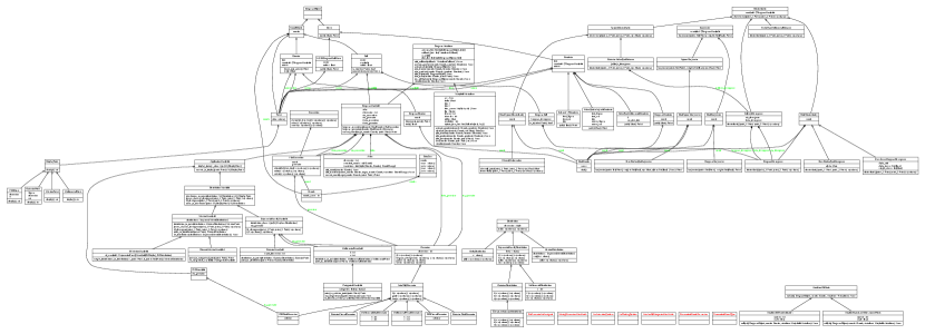
Appendix A Full Class Diagram
