Probability Passing for Graph Neural Networks: Graph Structure and Representations Joint Learning

Abstract

Graph Neural Networks (GNNs) have achieved notable success in the analysis of non-Euclidean data across a wide range of domains. However, their applicability is constrained by the dependence on the observed graph structure. To solve this problem, Latent Graph Inference (LGI) is proposed to infer a task-specific latent structure by computing similarity or edge probability of node features and then apply a GNN to produce predictions. Even so, existing approaches neglect the noise from node features, which affects generated graph structure and performance. In this work, we introduce a novel method called Probability Passing to refine the generated graph structure by aggregating edge probabilities of neighboring nodes based on observed graph. Furthermore, we continue to utilize the LGI framework, inputting the refined graph structure and node features into GNNs to obtain predictions. We name the proposed scheme as Probability Passing-based Graph Neural Network (PPGNN). Moreover, the anchor-based technique is employed to reduce complexity and improve efficiency. Experimental results demonstrate the effectiveness of the proposed method.

1 Introduction

Graph neural networks (GNNs) have gained considerable attention in recent years for their efficiency in analyzing graph data across various real-world applications [5, 13, 10, 30], such as microscopic molecular networks [16], protein networks [26], as well as macroscopic social networks, traffic networks [32], and industrial chain [18]. In the aforementioned scenarios, it is assumed that the observed graph structure is optimal for downstream task. However, the observed graph may be full of noise [8] and incompleteness, stemming from errors in data collection or measurement. For instance, in studies on the toxicity of compounds, it is challenging to regress the toxicity of compounds based on molecular graphs [16]. Similarly, in the domain of macroscopic social networks, connections among individuals on social media may not effectively reflect their underlying relevance.

To this end, Latent Graph Inference (LGI)  [12, 2, 7, 36] is proposed to jointly learn the latent graph and corresponding node embeddings using graph learner and GNNs. Specifically, the graph learner first computes the similarity or edge probabilities between node pairs , and then generates graph structure via sampling from edge distribution. Subsequently, GNNs take the node features and the generated graph as input to produce the predictions for downstream tasks. LGI plays a vital role in improving predictive performance by rectifying the process of aggregating neighbor information [28, 12]. Unfortunately, there exist two weaknesses that may limit its performance. Firstly, these models assume that the node features are noiseless and that graph noise only arises from graph topology, neglecting the impact of noise from node features. Secondly, it’s expensive to compute similarity or probabilities for all node pairs.

Figure 1: A sketch of the proposed Probability Passing. The blue bar charts represent the edge probability distributions. The red node and yellow nodes represent the central node and its neighbors respectively.

Figure 2: The interpretation of Probability Passing from the perspective of a two-step transition probability. The observed adjacency matrix can be viewed as a 0-1 probability matrix. In this example, the generated edge probability distribution is uniform, and the green nodes represent nodes that are not connected to the central node. The final probability from the central node to the target node is obtained through a special form of two-step transition probabilities generated by the adjacency matrix and the generated probability matrix.

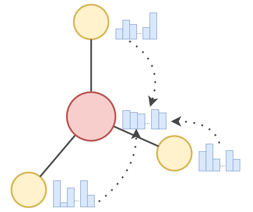
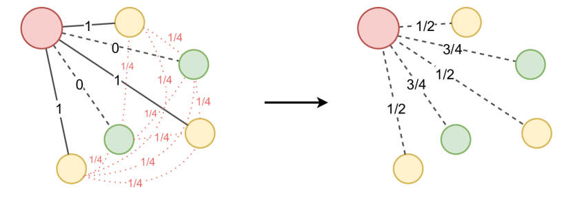
To address the first issue, we propose an innovative approach named Probability Passing, similar to Message Passing. As illustrated in fig. 2, this method updates the probability distribution of the central node with other nodes by aggregating the probability distributions of neighboring nodes along the observed graph structure, which means that if two nodes are directly connected in the observed graph, the edge probabilities between the pairs of them and a third node will be similar. It allows to correct the inaccurate edges and add the missing edges in the generated graph structure. In addition, we can explain Probability Passing from the respective of transition probability as shown in fig. 2. Typically, when computing two-step transition probabilities, two identical probability matrices are used. In the case of Probability Passing, the adjacency matrix can be treated as a 0-1 probability matrix. Probability transfer is performed on the adjacency matrix, and then on the generated probability matrix, resulting in the regeneration of the probability matrix.

To address the second problem, we develop anchor-based method [2, 19, 35]. Specifically, we initially randomly sample from nodes to produce anchors. Subsequently, for every node, we calculate the edge probability between this node and the corresponding anchors. Leveraging this probability, we differentiably sample the edges to obtain the generated graph structure. The anchor-based method not only reduces the time and memory complexity, but also improves efficiency. Intuitively, anchors play as message relay stations, responsible for receiving information and passing it.

To summarize, we outline the main contributions of this paper as follows:

• We propose a novel Probability Passing method, which updates the edge probability distribution of central nodes by aggregating edge probabilities of neighbors along the observed graph structure.

• The anchor-based method presented in this paper offers an efficient approach reducing both time and memory complexity while improving efficiency by utilizing anchors as message relay stations.

• We have validated the effectiveness and robustness of the model on real-world datasets.

2 Related Work

GNNs have emerged as crucial tools for processing structured graph data, and achieved significant success in various domains such as social networks [9], bioinformatics [15] and recommendation systems [37]. Traditional GNNs are typically used under the assumption of a complete and accurate graph structure. However, in practical applications, one of the challenges is that the initial graph may be unavailable, incomplete, or full of noise.

In scenarios where the initial graph is not given or incomplete, people have to dynamically extract structural information from the features. This requires modeling the connectivity patterns of the graph during the inference process. For instance, [33] proposed the EdgeConv model to handle point cloud data, which lacks explicit edge information. EdgeConv combined point cloud networks and edge convolutions to construct the graph structure. Similarly,  [8] proposed to learn latent discrete structures by jointly learning the graph structure and GNN parameters through two levels of optimization problems. The outer-level problem aims to learn the graph structure, and the inner-level problem involves optimizing model parameters in each iteration of the outer-level problem. This approach successfully handles the application of GNNs in scenarios with incomplete or damaged graphs.

In scenarios where the observed graph data contains noise, graph fusion including multi-modal graph fusion [17, 6, 34, 1, 21] and fusing observed graphs with inference graphs [2, 27, 12, 4, 23] prove to be effective methods.

Multi-modal methods have demonstrated the potential to learn an accurate graph based on multiple observed graphs. For example, [17] proposed the Multimodal Fusion Graph Convolutional Network (MFGCN) model to extract spatial patterns from geographical, semantic, and functional relevance, which has been applied in accurate predictions for online taxi services.  [6] presented multi-modal graph AI methods that combine different inductive preferences and leverage graph processing for cross-modal dependencies.  [34] proposed a graph neural network model to fuse two-modal brain graphs based on diffusion tensor imaging (DTI) and functional magnetic resonance imaging (fMRI) data for the diagnosis of ASD (Autism Spectrum Disorder). In [1], the authors consider continual graph learning by proposing the Multi-modal Structure-Evolving Continual Graph Learning (MSCGL) model, aiming to continually adapt their method to new tasks without forgetting the old ones. [23] utilized graph reconstruction in both feature space and structural space for clustering, effectively addressing the challenges associated with handling heterogeneous graphs. The aforementioned multi-modal methods ignore potential modal discrepancies. To address this issue, [21] proposed an adversarial encoder-decoder-classifier to explore interactions among different modalities.

Another feasible approach is to learn a latent graph and integrate it with the initial graph. For instance, [2] introduced the Iterative Deep Graph Learning (IDGL) model to learn an optimized graph structure. [27] proposed a Graph Structure Learning framework guided by the Principle of Relevant Information (PRI-GSL) to identify and reveal hidden structures in a graph. [12] introduced the Differentiable Graph Module (DGM), a learnable function that predicted edge probabilities in a graph, enabling the model to dynamically adjust the graph structure during the learning process. Furthermore, [4] generalized the Discrete Deep Generative Model(dDGM) for latent graph learning.

3 Method

3.1 Preliminary and Problem Definition

We denote a graph as $\mathcal{G}=(\mathcal{V},\mathcal{E})$ where the node set $\mathcal{V}$ comprises $N$ nodes, and the edge set $\mathcal{E}=$ $\{(i,j)\mid a_{ij}=1\}$ is defined by an initial noisy adjacency matrix $\mathbf{A}^{(0)}=[a_{ij}]_{N\times N}$, where $a_{ij}=1$ if nodes $i$ and $j$ are connected, and 0 otherwise. Each node has an input feature $\mathbf{x}\in\mathbb{R}^{D}$ and a label $\mathbf{y}.$ This paper primarily centers on the exploration of graph representation learning in the context of noisy graph structure and features. In this setting, given a noisy graph input $\mathcal{G}:=\{\mathbf{A}^{(0)},\mathbf{X}\}$, the graph structure learning problem is to produce an optimized graph $\mathcal{G}^{*}:=\{\mathbf{A}^{(*)},\mathbf{X}\}$ and node embeddings $\mathbf{H}=\text{GNN}(\mathcal{G}^{*},\mathbf{X})$, with respect to the downstream tasks.

Figure 3: Illustration of the proposed modcel and its data flow. The input graph data entails node features $\mathbf{X}$ and graph adjacency $\mathbf{A}^{(0)}$. The entire model is divided into two parts: graph structure learning and node representations learning. In the graph structure learning process section 3.3, Probability Learning receives $\mathbf{X}$ and $\mathbf{A}^{(0)}$ to produce the probability matrix $\mathbf{P}$. Through probability passing, the probability matrix and the original adjacency matrix are fused, and finally $\mathbf{A}^{(*)}$ is obtained after sparsification. The node representations learning process in algorithm 1 uses GCN as message-passing method to generate predictions.

3.2 Network Architecture

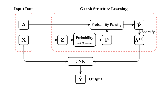
PPGNN consists of two components: 1) graph learning, and 2) node representation learning. Figure 3 illustrates these components. In the next two subsections, we will explain them. Lastly we describe how graph structure and node representations can be jointly learned.

3.3 Probability Passing for Graph Learning

Graph structure learning aims to jointly learn the graph structure and corresponding embeddings. Given node features, graph structure learning first models the edge probabilities between node pairs. Previous methods construct edge probabilities solely using node features. However, if there is noise in the node features, it will affect the probability matrix. To address this issue, we use the observed graph to correct the probability metric, increasing the probability of edges that truly exist and decreasing the probability of edges that do not.

Node-node probability learning. Common options include gaussian kernel  [12] and attention mechanism [11, 29]. Similar to [12], we use gaussian kernel as stated in eq. 1.

$$\mathbf{z}_{i}=\text{f}_{\Phi}(\mathbf{x}_{i})\text{,}\quad\mathbf{p}_{ij}=e^{-\|\mathbf{z}_{i}-\mathbf{z}_{j}\|^{2}/t}\text{,}$$ (1)

where the function $\text{f}_{\Phi}$, a neural layer mapping input into the latent space, can be a GNN or shallow MLP. Here, $\mathbf{\Phi}$ and $t$ are learnable parameters, $\|\cdot\|$ is $L$-2 norm. Furthermore, to mitigate the impact of noise in the features on the results, we adopt a novel approach called probability passing to refine the probability metric. Similar to message passing, it aggregates the probabilities of neighboring nodes to the central node on $\mathbf{A}^{(0)}$. We define probability passing as:

$$\hat{\mathbf{P}}=\mathbf{D}^{-1}\mathbf{A}^{(0)}\mathbf{P}\text{,}$$ (2)

where $\mathbf{P}\in\mathbb{R}^{N\times N}$ is a matrix composed of elements $\mathbf{p}_{ij}$ and $\mathbf{D}$ is the degree matrix of $\mathbf{A}^{(0)}$.

Node-anchor probability learning. The above probability metric learning function like eq. 1 computes edge probabilities for all pairs of graph nodes, which requires $\mathcal{O}(N^{2})$ complexity for both computational time and memory consumption. To address this issue, we design the anchor-based probability metric learning technique, which learns a node-anchor probability matrix $\mathbf{R}\in\mathbb{R}^{N\times s}$ ($s$ is the number of anchors and hyperparameter), inspired by [2]. This process only consumes $\mathcal{O}(Ns)$, achieving linear complexity.

Specifically, we first randomly sample $s$ anchors from $\mathcal{V}$ to form the set $\mathcal{U}$. Therefore, the Node-anchor probability matrix $\mathbf{R}$ can be computed by

$$\mathbf{r}_{ij}=e^{-\|\mathbf{z}_{i}-\mathbf{z}_{u}\|^{2}/t}\text{,}$$ (3)

where $\mathbf{z}_{u}$ is the embedding of anchor node. To further correct probability matrix, we use probability passing:

$$\hat{\mathbf{R}}=\mathbf{D}^{-1}\mathbf{A}^{(0)}\mathbf{R}\text{.}$$ (4)

Graph sparsification via Gumble-Top-$k$ trick. In the real world, the adjacency matrix of a graph is generally sparse. However, $\hat{\mathbf{P}}$ from eq. 2 and $\hat{\mathbf{R}}$ from eq. 4 are dense, which not only lowers computational efficiency but also degrades performance. Therefore, we employ the Gumbel-Top-$k$ trick [14] to sparsify $\hat{\mathbf{P}}$ or $\hat{\mathbf{R}}$ to obtain a new adjacency matrix $\mathbf{A}^{(*)}$.

Specifically, for each node $i$, we extract $k$ edges as the first $k$ elements of $\log(\mathbf{s}_{i})-\log(-\log(\mathbf{q}))$, where $\mathbf{q}\in\mathbb{R}^{N}$ is uniformly independently distributed in the interval $[0,1]$ and $\mathbf{s}_{i}$ represents the probability scores vector for node $i$ and other nodes(or anchors), i.e.,the $i$-th row of $\hat{\mathbf{P}}$ or $\hat{\mathbf{R}}$.

3.4 Node Representation Learning

Algorithm 1 General Framework For PPGNN

  Input: Node feature matrix $\mathbf{X}$, adjacency matrix $\mathbf{A}^{(0)}$

  Output: Predicted node labels $\hat{\mathbf{y}}$

  if PPGNN then

     $\mathbf{P}\leftarrow\text{ProbabilityLearning}(\mathbf{X},\mathbf{A}^{(0)}$) using eq. 1

     $\hat{\mathbf{P}}\leftarrow\text{ProbabilityPassing}(\mathbf{A}^{(0)},\mathbf{P}$) using eq. 2

     $\mathbf{A}^{(*)}\leftarrow\text{Gumble-top-}k(\hat{\mathbf{P}})$

     for $l\in\{0,1,\cdots,L-1\}$ do

        $\mathbf{U}^{(l)}\leftarrow\text{GNN}(\mathbf{A}^{(*)},\mathbf{U}^{(l-1)};\mathbf{W}^{(l)})$

     end for

  else if PPGCN-anchor then

     $\mathbf{R}\leftarrow\text{ProbabilityLearning}(\mathbf{X},\mathbf{A}^{(0)}$) using eq. 3

     $\hat{\mathbf{R}}\leftarrow\text{ProbabilityPassing}(\mathbf{A}^{(0)},\mathbf{R}$) using eq. 4

     $\mathbf{A}^{(*)}\leftarrow\text{Gumble-top-}k(\hat{\mathbf{R}})$

     for $l\in\{0,1,\cdots,L-1\}$ do

        $\mathbf{V}^{(l)}\leftarrow\text{MP}_{1}(\mathbf{U}^{(l-1)},\mathbf{A}^{(*)})$ using eq. 6

        $\mathbf{U}^{(l)}\leftarrow\text{MP}_{2}(\mathbf{V}^{(l)},\mathbf{A}^{(*)};\mathbf{W}^{(l)})$ using eq. 7

     end for

  end if

  $\hat{\mathbf{y}}\leftarrow\text{MLP}(\mathbf{U}^{(L)})$

  Update $\{\mathbf{\Phi},t,\mathbf{W}^{(l)}\}$ with $\mathcal{L}$ using section 3.5

Node representation learning and graph learning are two separate processes that do not interfere with each other. In this paper, we utilize an $L$-layer GCN to learn node features, which accepts $\mathbf{A}^{(*)}$ in section 3.3 and $\mathbf{X}$ as inputs,

$$\mathbf{U}^{(l)}=\text{GNN}(\mathbf{A}^{(*)},\mathbf{U}^{(l-1)};\mathbf{W}^{(l)})\text{,}$$ (5)

where $\mathbf{U}^{(0)}=\mathbf{X}$ and $\mathbf{U}^{(L)}$ at the final layer $L$ is the output. $\mathbf{U}^{(L)}$ contains the necessary information of the downstream tasks. $\mathbf{W}^{(l)}$ is the parameter matrix of layer $l=1,2,...,L$.

If $\mathbf{A}^{(*)}$ is obtained by anchor-based probability metric learning technique, we need to employ tow-step message passing [2]. The first step is formulated by eq. 6 involving aggregating messages from nodes to anchor points to obtain anchor features $\mathbf{V}$. The second step is formulated by eq. 7 involving aggregating messages from anchor points to nodes to update node embeddings $\mathbf{U}$.

$$\mathbf{V}^{(l)}=\text{MP}_{1}(\mathbf{U}^{(l-1)},\mathbf{A}^{(*)})=\Lambda^{-1}\mathbf{A}^{(*)^{\top}}\mathbf{U}^{(l-1)}\text{,}$$ (6)

$$\mathbf{U}^{(l)}=\text{MP}_{2}(\mathbf{V}^{(l)},\mathbf{A}^{(*)})=\Delta^{-1}\mathbf{A}^{(*)}\mathbf{V}^{(l)}\text{,}$$ (7)

where $\Lambda$ and $\Delta$ are diagonal matrices defined as $\Lambda_{kk}=\sum_{j^{\prime}=1}^{n}\mathbf{A}^{(*)}_{j^{\prime}k}$ and $\Delta_{ii}=\sum_{k^{\prime}=1}^{s}\mathbf{A}^{(*)}_{ik^{\prime}}$ respectively.

3.5 Graph and Node Representation Joint Learning

The parameters within the graph learning module, i.e., $\mathbf{\Phi}$ and $t$, cannot be optimized solely through cross-entropy loss $\mathcal{L}_{pred}$.To optimize the graph learning, we introduce a graph loss, as described in [12], which rewards edges contributing to correct classification and penalizes edges leading to misclassification.

Let $\hat{\mathbf{y}}=(\hat{y}_{1},\cdots,\hat{y}_{i})$ denotes node labels predicted by our model and the vector of truth labels is denoted as $\mathbf{y}$. The graph loss function is as follows,

$$\mathcal{L}_{\mathcal{G}}=\sum_{i=1}^{N}\sum_{j\in\mathcal{N}_{i}(\mathbf{A})}\delta(y_{i},\hat{y}_{i})\log{s}_{ij}(\mathbf{\Phi},t)$$ (8)

where ${s}_{ij}$ is the element of $\hat{\mathbf{P}}$ or $\hat{\mathbf{R}}$. Additionally, $\delta\left(y_{i},\hat{y}_{i}\right)$ denotes the reward function, indicating the difference between the average predicted accuracy and the current accuracy for node $i$. Specifically, $\delta(y_{i},\hat{y}_{i})=\mathbb{E}((c_{i}))-c_{i}$, where $c_{i}=1$ if $\hat{y}_{i}=y_{i}$ and 0 otherwise.

Then we propose to jointly learning the graph structure and node representation by minimizing a hybrid loss function combining the cross-entropy loss $\mathcal{L}_{pred}$ and the graph loss $\mathcal{L}_{\mathcal{G}}$, namely, $\mathcal{L}=\mathcal{L}_{pred}+\mathcal{L}_{\mathcal{G}}$.

The algorithm 1 represents the computational procedure of the proposed model.

4 Experiment

In this section, we study the benefits of the PPGNN and compare it with state-of-the-art methods on node classification task.

4.1 Datasets and Setup

We use four popular graph datasets: Cora, PubMed, CiteSeer [24], and Photo [25]. The first three, Cora, PubMed, and CiteSeer, are citation datasets, where nodes represent scientific publications described by word vectors, and edges denote citation relationships between nodes. On the other hand, Photo is segments of the Amazon co-purchase graph [22], where nodes represent goods described by bag-of-words encoded product reviews, and edges indicate items that are frequently bought together. Please refer to table 1 for detailed statistics of datasets.

In this experiment, we focus on the transductive node classification task, where all nodes are observed during training but only the train set has labels. For our model, GCN is used as aggregate function with three layers having hidden dimensions of 64. Training involves the Adam optimizer with a learning rate set at $5\times 10^{-3}$. The train/validation/test splits and all other settings follow [12]. For each dataset, we execute 5 runs with different random seeds and report the mean accuracy and standard deviation. All our experiments are conducted on the NVIDIA RTX 3090 24GB GPU.

Table 1: Summary of datasets

	Cora	CiteSeer	PubMed	Photo
# Nodes	2708	3327	19717	7650
# Edges	5278	4552	44324	119081
# Features	1433	3703	500	745
# Classes	7	6	3	8
Average Degree	3.9	2.7	4.5	31.1

4.2 Baselines

To evaluate our method, we consider some baselines as follows,

1. MLP (Multi-layer Perceptron) : MLP neglects the graph structure.

2. Classical GNNs.

   • GCN (Graph Convolutional Network) [13]: GCN performs a simple diffusion operation over node features;

   • GAT (Graph Attention Network) [31]: GAT refines the diffusion process by learning per-edge weights through an attention mechanism.

3. Latent graph inference models that only accept node features as the input.

   • $k$NN-GCN: $k$NN-GCN constructs a $k$NN (sparse $k$-nearest neighbor) graph based on node feature similarities and subsequently feeds it into GCN;

   • SLAPS [7]: SLAPS provides more supervision for inferring a graph structure through self-supervision.

4. Latent graph inference models that accept node features and original graph structure.

   • LDS [8]: LDS jointly learns the graph structure and parameters of a GCN;

   • IDGL [3] : IDGL jointly and iteratively learns graph structure and graph embedding

   • IDGL-ANCH [2] : IDGL-ANCH is a variant of IDGL, which reduces time complexity through anchor-based approximation [20];

   • dDGM [12]: dDGM is a learnable function that predicts a sparse adjacency matrix which is optimal for downstream task. We use Euclidean and hyperbolic space geometries for the graph embedding space with GCN as the aggregation function, denoted as dDGM-E and dDGM-H, respectively;

   • dDGM-EHH and dDGM-SS [4]: dDGM-EHH and dDGM-SS incorporates Riemannian geometry into the dDGM, representing embedding spaces with a torus and a manifold of Euclidean plane and two hyperboloids.

4.3 Performance

Table 2: Results of accuracy on nodes classification task for the baselines and the proposed method. We report the mean and standard deviation (in percent) of accuracy on 5 runs for MLP, GCN, GAT and our model, as well as all for Photo. The others are obtained from the respective official reports. OOM indicates out of memory, OOT indicates out of time.

Methods	Cora	CiteSeer	PubMed	Photo
MLP	$62.98_{\pm 2.624}$	$65.06_{\pm 3.469}$	$85.26_{\pm 0.633}$	$69.60_{\pm 3.800}$
GCN	$78.74_{\pm 1.250}$	$67.74_{\pm 1.723}$	$83.60_{\pm 1.233}$	$92.82_{\pm 0.653}$
GAT	$80.10_{\pm 1.672}$	$67.74_{\pm 1.723}$	$82.56_{\pm 1.436}$	$91.80_{\pm 1.428}$
$k$NN-GCN	$66.50_{\pm 0.400}$	$68.30_{\pm 1.300}$	$70.40_{\pm 0.400}$	$78.28_{\pm 1.676}$
SLAPS	$74.20_{\pm 0.500}$	$73.10_{\pm 1.000}$	$74.30_{\pm 1.400}$	$46.72_{\pm 0.110}$
LDS	$84.08_{\pm 0.400}$	$75.04_{\pm 0.400}$	OOT	OOT
IDGL	$84.50_{\pm 0.300}$	$74.10_{\pm 0.200}$	OOM	$90.13_{\pm 0.200}$
IDGL-ANCH	$84.40_{\pm 0.200}$	$72.00_{\pm 1.000}$	$83.00_{\pm 0.200}$	$87.60_{\pm 0.320}$
dDGM-E	$84.60_{\pm 0.852}$	$74.80_{\pm 0.924}$	$87.60_{\pm 0.751}$	$93.06_{\pm 0.670}$
dDGM-H	$84.40_{\pm 1.700}$	$74.60_{\pm 0.763}$	$86.60_{\pm 0.952}$	$91.48_{\pm 2.871}$
dDGM-EHH	$86.63_{\pm 3.250}$	$75.42_{\pm 2.390}$	$39.93_{\pm 1.350}$	$--$
dDGM-SS	$65.96_{\pm 9.460}$	$59.16_{\pm 5.960}$	$87.82_{\pm 0.590}$	$--$
PPGNN	$87.10_{\pm 0.326}$	$76.34_{\pm 0.580}$	$\bm{88.40_{\pm 0.770}}$	$\bm{93.40_{\pm 0.604}}$
PPGNN-anchor	$\bm{88.60_{\pm 0.960}}$	$\bm{78.08_{\pm 0.810}}$	$74.08_{\pm 2.07}$	$90.60_{\pm 0.450}$

Results. The results of the baselines and the proposed model are reported in Table 2. The results of baselines, excluding MLP, GAT, GCN and the results on the Photo, are sourced from the respective official reports. We can see that our model consistently outperforms all baselines on four datasets, indicating the efficacy of the proposed method.

Firstly, we compare MLP with $k$NN-GCN and SLAPS, which rely solely on node features. It is observed that $k$NN-GCN and SLAPS perform better than MLP on Cora and CiteSeer but worse on PubMed and Photo. This emphasizes the importance of graph structure, with a lower-quality graph structure negatively impacting model performance.

Further comparison of latent graph inference models involves those utilizing only node features ($k$NN-GCN, SLAPS) and those using both node features and the original graph (LDS, IDGL, dDGM). It is worth noting that LDS, IDGL, and dDGM incorporate the original graph as part of their input and achieve better performance than the methods that only utilize node features. This suggests that the collaborative use of both original graph structures and node features contributes to the performance.

We explore different graph embedding spaces within dDGM models (dDGM-E, dDGM-H, dDGM-EHH, dDGM-SS). Among them, dDGM-EHH performs best on Cora and CiteSeer, while dDGM-SS performs best on PubMed. This indicates that the choice of embedding space impacts the similarity measurement matrix and latent graph structures. To further demonstrate the superiority of our proposed PPGNN, we compare it with dDGM-E. We observe a significant performance improvement in our model. This indicates PPGNN can help to avoid learning the wrong latent graph structures when the depth is not enough.

(a) Cora

(b) CiteSeer

Figure 4: Test accuracy ($\pm$ standard deviation ) in percent for the edge addition and deletion on Cora and CiteSeer.

Figure 5: The ratio of two nodes in the test set sharing the same label in different probability interval.

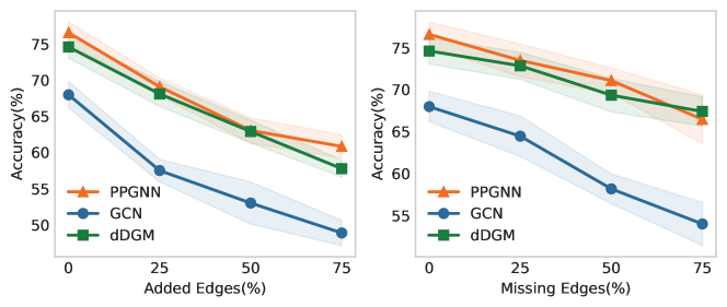
Robustness. To assess the robustness of PPGNN, we construct graphs with random edges deletion and addition on Cora and CiteSeer as shown in Figure 4 (a) and (b) respectively. Specifically, we add or remove edges at ratios 25%, 50%, and 75% to the existing edges for each dataset. Compared to GCN and dDGM, PPGNN achieves better results in both scenarios. Especially in scenarios involving edge addition, PPGNN consistently demonstrates outstanding performance across all ratios, showcasing its robust ability to eliminate noise from the graph.

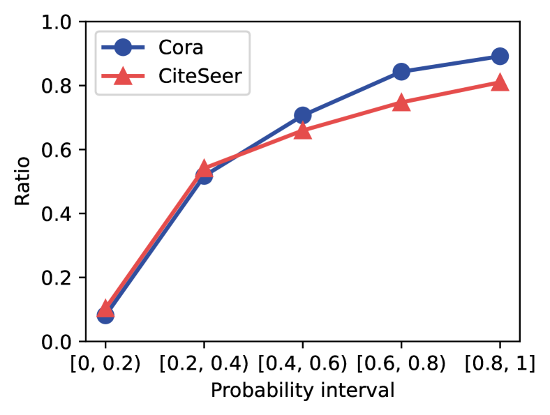
Homophily. We compute the ratio of the number of nodes pairs with the same label to the total number of nodes pairs in different probability intervals, using the test set of Cora and CiteSeer, as shown in Figure 5. We can see that the higher the probability of a connection between two nodes by eq. 2, the more likely it is that their labels are consistent. This indicates that PPGNN effectively captures and reinforces homophilic relationships in the graph structure.

4.4 Model Analysis

4.4.1 Aggregate function

In our analysis of aggregate functions, we consider three options: GCN [13], GAT [30], and EdgeConv [33]. The results, as depicted in table 3, show comparable performance between GCN and GAT, with no significant difference. However, the adoption of EdgeConv notably reduces accuracy, particularly on small datasets.

This observation can be explained by the fact that a latent graph structure obtained through Probability Passing module already incorporates the information about nodes interactions. Therefore, GAT does not significantly contribute to performance improvement. Additionally, during the training process of our model, each sampled latent graph varies, making it challenging for the loss involving edge attributes to converge. Consequently, the use of EdgeConv leads a decrease in accuracy.

Table 3: Results of our model with different aggregate fuctions. We report the mean and standard deviation (in percent) of the accuracy on 5 runs.

$\text{Aggre}(\cdot)$	Cora	CiteSeer	PubMed
GCN	$87.10_{\pm 0.326}$	$\mathbf{76.34_{\pm 0.580}}$	$\mathbf{88.40_{\pm 0.770}}$
GAT	$\mathbf{87.30_{\pm 1.020}}$	$76.22_{\pm 1.130}$	$88.20_{\pm 0.704}$
EdgeConv	$55.70_{\pm 5.100}$	$52.44_{\pm 2.890}$	$86.08_{\pm 0.900}$

4.4.2 Time Complexity

As for PPGNN, the cost of learning a probability matrix is $\mathcal{O}(N^{2}h)$ for $N$ nodes and embeddings in $\mathbb{R}^{h}$. Direct matrix multiplication in eq. 2 has a computational complexity of $\mathcal{O}(N^{3})$. However, considering the sparsity of matrix $\mathbf{A}$, employing sparse matrix multiplication reduces the complexity to $\mathcal{O}(\|A^{(0)}\|N)$, where $\|A^{(0)}\|$ denotes the number of edges in the generated graph structure. Hence the total complexity is $\mathcal{O}(N^{2}h+\|A^{(0)}\|N)$ in graph structure learning process.

As for PPGNN-anchor, the cost of learning a node-anchor probability is $\mathcal{O}(Nsh)$.While computing the result of Probability Passing in eq. 4 costs $\mathcal{O}(N^{2}s)$. We can employ the sparse matrix multiplication to reduce the complexity to $\mathcal{O}(\|A^{(0)}\|s)$. The overall time complexity is $\mathcal{O}(Nsh+\|A^{(0)}\|s)$($s\ll n$).

5 Conclusion

The graph structure is very important for GNNs. Many studies on latent graph inference have confirmed that is prevalent in popular graph datasets. The noise in generated graph tends to be amplified during the message-passing process, impacting the performance of GNNs. To address this issue, this paper introduces Probability Passing to improve performance. Our experimental results on four widely-used graph datasets for nodes classification task demonstrate the superior performance of our proposed model.

However, this method still has limitations. For instance, its computational complexity depends on the edges of the observed graph (if the observed graph has too many edges, it will affect computational efficiency). Additionally, this method can only be applied when the observed graph is available. It is not suitable for cases where the observed graph is unknown and where the generated graph structure from node features contains obvious noise.

In this study, we adopt the Probability Passing to correct the generated graph structure, which is similar to residual connection but is applied to non-Euclidean data. Besides that, it would be interesting to explore other methods to construct graph structure. We hope our work can inspire more researches into latent graph inference, able to infer graphs that are closer to the true underlying graph.

References

- [1] Jie Cai, Xin Wang, Chaoyu Guan, Yateng Tang, Jin Xu, Bin Zhong, and Wenwu Zhu. Multimodal continual graph learning with neural architecture search. In Proceedings of the ACM Web Conference 2022, pages 1292–1300, 2022.
- [2] Yu Chen, Lingfei Wu, and Mohammed Zaki. Iterative deep graph learning for graph neural networks: Better and robust node embeddings. Advances in neural information processing systems, 33:19314–19326, 2020.
- [3] Yu Chen, Lingfei Wu, and Mohammed J Zaki. Deep iterative and adaptive learning for graph neural networks. arXiv:1912.07832, 2019.
- [4] Haitz Sáez de Ocáriz Borde, Anees Kazi, Federico Barbero, and Pietro Lio. Latent graph inference using product manifolds. In The Eleventh International Conference on Learning Representations, 2023.
- [5] Michaël Defferrard, Xavier Bresson, and Pierre Vandergheynst. Convolutional neural networks on graphs with fast localized spectral filtering. In Proceedings of the Thirtieth International Conference on Neural Information Processing Systems, NeurIPS, page 3844–3852, 2016.
- [6] Yasha Ektefaie, George Dasoulas, Ayush Noori, Maha Farhat, and Marinka Zitnik. Multimodal learning with graphs. Nature Machine Intelligence, 5(4):340–350, 2023.
- [7] Bahare Fatemi, Layla El Asri, and Seyed Mehran Kazemi. Slaps: Self-supervision improves structure learning for graph neural networks. Advances in Neural Information Processing Systems, 34:22667–22681, 2021.
- [8] Luca Franceschi, Mathias Niepert, Massimiliano Pontil, and Xiao He. Learning discrete structures for graph neural networks. In International conference on machine learning, pages 1972–1982. PMLR, 2019.
- [9] Zhiwei Guo and Heng Wang. A deep graph neural network-based mechanism for social recommendations. IEEE Transactions on Industrial Informatics, 17(4):2776–2783, 2020.
- [10] Will Hamilton, Zhitao Ying, and Jure Leskovec. Inductive representation learning on large graphs. In NeurIPS, pages 1025–1035, 2017.
- [11] Bo Jiang, Ziyan Zhang, Doudou Lin, Jin Tang, and Bin Luo. Semi-supervised learning with graph learning-convolutional networks. In 2019 IEEE/CVF Conference on Computer Vision and Pattern Recognition (CVPR), Jun 2019.
- [12] Anees Kazi, Luca Cosmo, Seyed-Ahmad Ahmadi, Nassir Navab, and Michael M Bronstein. Differentiable graph module (dgm) for graph convolutional networks. IEEE Transactions on Pattern Analysis and Machine Intelligence, 45(2):1606–1617, 2022.
- [13] Thomas N. Kipf and Max Welling. Semi-supervised classification with graph convolutional networks. In ICLR, 2017.
- [14] Wouter Kool, Herke Van Hoof, and Max Welling. Stochastic beams and where to find them: The gumbel-top-k trick for sampling sequences without replacement. In International Conference on Machine Learning, pages 3499–3508. PMLR, 2019.
- [15] Rui Li, Xin Yuan, Mohsen Radfar, Peter Marendy, Wei Ni, Terrence J O’Brien, and Pablo M Casillas-Espinosa. Graph signal processing, graph neural network and graph learning on biological data: a systematic review. IEEE Reviews in Biomedical Engineering, 16:109–135, 2021.
- [16] Ruoyu Li, Sheng Wang, Feiyun Zhu, and Junzhou Huang. Adaptive graph convolutional neural networks. In Proceedings of the AAAI conference on artificial intelligence, 2018.
- [17] Lyuchao Liao, Ben Li, Fumin Zou, and Dejuan Huang. Mfgcn: A multimodal fusion graph convolutional network for online car-hailing demand prediction. IEEE Intelligent Systems, 38(3):21–30, 2023.
- [18] Bin Liu, Jiujun He, Ziyuan Li, Xiaoyang Huang, Xiang Zhang, and Guosheng Yin. Interpret esg rating’s impact on the industrial chain using graph neural networks. In Proceedings of the Thirty-Second International Joint Conference on Artificial Intelligence, IJCAI-23, pages 6076–6084, 8 2023. AI for Good.
- [19] Wei Liu, Junfeng He, and Shih-Fu Chang. Large graph construction for scalable semi-supervised learning. Proceedings of the 27th international conference on machine learning (ICML-10), pages 679–686, 2010.
- [20] Wei Liu, Junfeng He, and Shih-Fu Chang. Large graph construction for scalable semi-supervised learning. In Proceedings of the 27th international conference on machine learning (ICML-10), pages 679–686, 2010.
- [21] Sijie Mai, Haifeng Hu, and Songlong Xing. Modality to modality translation: An adversarial representation learning and graph fusion network for multimodal fusion. In Proceedings of the AAAI Conference on Artificial Intelligence, pages 164–172, 2020.
- [22] Julian McAuley, Christopher Targett, Qinfeng Shi, and Anton Van Den Hengel. Image-based recommendations on styles and substitutes. In Proceedings of the 38th international ACM SIGIR conference on research and development in information retrieval, pages 43–52, 2015.
- [23] Erlin Pan and Zhao Kang. Beyond homophily: Reconstructing structure for graph-agnostic clustering. In Proceedings of the 40th International Conference on Machine Learning, volume 202 of Proceedings of Machine Learning Research, pages 26868–26877. PMLR, 23–29 Jul 2023.
- [24] Prithviraj Sen, Galileo Namata, Mustafa Bilgic, Lise Getoor, Brian Galligher, and Tina Eliassi-Rad. Collective classification in network data. AI magazine, 29(3):93–93, 2008.
- [25] Oleksandr Shchur, Maximilian Mumme, Aleksandar Bojchevski, and Stephan Günnemann. Pitfalls of graph neural network evaluation. arXiv preprint arXiv:1811.05868, 2018.
- [26] Alexey Strokach, David Becerra, Carles Corbi-Verge, Albert Perez-Riba, and Philip M Kim. Fast and flexible protein design using deep graph neural networks. Cell systems, 11(4):402–411, 2020.
- [27] Qingyun Sun, Jianxin Li, Beining Yang, Xingcheng Fu, Hao Peng, and S Yu Philip. Self-organization preserved graph structure learning with principle of relevant information. In Proceedings of the AAAI Conference on Artificial Intelligence, pages 4643–4651, 2023.
- [28] Jake Topping, Francesco Di Giovanni, Benjamin Paul Chamberlain, Xiaowen Dong, and Michael M. Bronstein. Understanding over-squashing and bottlenecks on graphs via curvature. In International Conference on Learning Representations, 2022.
- [29] Ashish Vaswani, Noam Shazeer, Niki Parmar, Jakob Uszkoreit, Llion Jones, AidanN. Gomez, Lukasz Kaiser, and Illia Polosukhin. Attention is all you need. Neural Information Processing Systems,Neural Information Processing Systems, Jun 2017.
- [30] Petar Velickovic, Guillem Cucurull, Arantxa Casanova, Adriana Romero, Pietro Liò, and Yoshua Bengio. Graph attention networks. In ICLR, 2018.
- [31] Petar Veličković, Guillem Cucurull, Arantxa Casanova, Adriana Romero, Pietro Liò, and Yoshua Bengio. Graph attention networks. In International Conference on Learning Representations, 2018.
- [32] Xiaoyang Wang, Yao Ma, Yiqi Wang, Wei Jin, Xin Wang, Jiliang Tang, Caiyan Jia, and Jian Yu. Traffic flow prediction via spatial temporal graph neural network. In Proceedings of the web conference 2020, pages 1082–1092, 2020.
- [33] Yue Wang, Yongbin Sun, Ziwei Liu, Sanjay E Sarma, Michael M Bronstein, and Justin M Solomon. Dynamic graph cnn for learning on point clouds. ACM Transactions on Graphics (tog), 38(5):1–12, 2019.
- [34] Lu Wei, Bin Liu, Jiujun He, Manxue Zhang, and Yi Huang. Autistic spectrum disorders diagnose with graph neural networks. In Proceedings of the 31st ACM International Conference on Multimedia, page 8819–8827, 2023.
- [35] Lingfei Wu, IanEn-Hsu Yen, Zhen Zhang, Kun Xu, Liang Zhao, Xi Peng, Yinglong Xia, and CharuC. Aggarwal. Scalable global alignment graph kernel using random features: From node embedding to graph embedding. arXiv: Learning,arXiv: Learning, Nov 2019.
- [36] Qitian Wu, Wentao Zhao, Zenan Li, David P Wipf, and Junchi Yan. Nodeformer: A scalable graph structure learning transformer for node classification. Advances in Neural Information Processing Systems, 35:27387–27401, 2022.
- [37] Shiwen Wu, Fei Sun, Wentao Zhang, Xu Xie, and Bin Cui. Graph neural networks in recommender systems: a survey. ACM Computing Surveys, 55(5):1–37, 2022.