Alpine: An adaptive language-agnostic pruning method for language models for code

Abstract

Language models of code have demonstrated state-of-the-art performance across various software engineering and source code analysis tasks. However, their demanding computational resource requirements and consequential environmental footprint remain as significant challenges. This work introduces Alpine, an adaptive programming language-agnostic pruning technique designed to substantially reduce the computational overhead of these models. The proposed method offers a pluggable layer that can be integrated with all Transformer-based models. With Alpine, input sequences undergo adaptive compression throughout the pipeline, reaching a size that is up to $\times 3$ less their initial size, resulting in significantly reduced computational load. Our experiments on two software engineering tasks, defect prediction and code clone detection across three language models CodeBert, GraphCodeBert and UniXCoder show that Alpine achieves up to a 50% reduction in FLOPs, a 58.1% decrease in memory footprint, and a 28.1% improvement in throughput on average. This led to a reduction in CO₂ by up to $44.85$%. Importantly, it achieves the reduction in computation resources while maintaining up to 98.1% of the original predictive performance. These findings highlight the potential of Alpine in making language models of code more resource-efficient and accessible while preserving their performance, contributing to the overall sustainability of adopting language models in software development. Also, it sheds light on redundant and noisy information in source code analysis corpora, as shown by the substantial sequence compression achieved by Alpine.

I Introduction

Transformer-based language models [1] were initially conceived for natural language understanding. Under the naturalness hypothesis [2], they were applied to solve diverse software engineering (se) tasks with remarkable accuracy. These tasks include code generation [3, 4, 5, 6], quality assurance [7, 8, 9, 10], maintenance [11, 12, 13, 14], and requirements engineering [15, 16].

Though the language models have shown exceptional promise, fine-tuning or running inference on these models require significant computational resources. Moreover, the demand of the resources is continuously increasing with the size of the language models. This entails that their training grows correspondingly, leading to increased usage of cloud computing services which operate on a pay-per-use basis. This inflates the direct financial investment for researchers and average users with consumer-grade hardware. In addition to the financial impact, the carbon footprint of training and maintaining these models is a growing environmental concern as they contribute to higher CO₂ emissions [17, 18, 19]. These issues underscore the urgency for more resource efficient algorithms.

Shi et al. [20] have proposed Compressor as a step towards this direction. Compressor combines task-specific knowledge distillation [21] and evolutionary search of network architecture to generate a configuration that yields a smaller model. Task-specific knowledge distillation often falls short in terms of task-specificity and computational overhead. The distilled student models are typically optimized for a specific task or domain, limiting their generalization abilities. Moreover, the process of task-specific knowledge distillation itself can be computationally expensive, as it involves fine-tuning the teacher model either way, generating predictions or soft labels, pre-training, and fine-tuning the student model.

Similarly, DietCode [22] attempts to achieve better resource utilization by assigning importance scores to tokens and statements based on attention weights, and then selecting the most important statements to form a new, condensed input. However, it has two main limitations. First, it relies on the peculiarities of task’s programming language, such as specific syntax, semantics, and constructs. This reliance makes extending the method to all programming languages difficult without overhead and customization. Second, it assumes that the attention weights remain static and applicable across different corpora and tasks. However, this is not the case given that these attention weights are derived from trainable parameters, which are updated when the language model is fine-tuned on other tasks.

To address the issues above, we introduce Alpine, a programming-language-independent pruning method that can be directly integrated into any Transformer-based model. As sequences go through the layers, Alpine prunes unimportant tokens that lay within a configurable range, reducing input size, and offering a considerable speedup during fine-tuning and inference. We evaluate Alpine on two software engineering tasks defect prediction and code clone detection using three language models, CodeBert, GraphCodeBert and UniXCoder. Our approach allows these models to use $\times 2$ less computation, measured by the number of floating point operations (flops) and memory footprint, with minimal loss in performance and even slight improvement in some scenarios.

This study makes the following contributions to the field.

• We conduct an analysis to quantify the computational requirements, measured by the flops, of the individual components within the Transformer model. The analysis helps us identify the bottleneck components and understand the changes in computational complexity with respect to the input sequence length.

• Using these insights, we design an effective pruning method that makes language models computationally efficient. Its plug-and-play characteristic makes it easy to integrate and use with virtually any Transformer-based model with minimal overhead.

• We illustrate how Alpine can maintain a considerable amount of the original accuracy exhibited by the none-pruned models with substantially less computation and carbon emission.

Alpine’s ability to reduce computational requirements while maintaining accuracy has two significant implications. First, it contributes to more sustainable software development practices by reducing the required computation and carbon footprint associated with such models. Second, it lowers the barriers to entry for developers and researchers, facilitating the adoption of language models for code, especially when constrained by consumer-grade gpus. As a result, it offers a more accessible and environmentally friendly solution for the software engineering community.
Replication package: Our replication package including source code and data is available online [23].

II Background and Motivation

II-A Transformer Architecture

The Transformer architecture, introduced by Vaswani et al. [1] for natural language processing (nlp), is a sequence-to-sequence model composed of two components: an encoder and a decoder. The focus of this work is on the encoder-only variant, one of the most used variants in SE-related tasks [24]. For the rest of the paper, we refer to a Transformer encoder layer by a Transformer layer for convenience.

Input Representation: The input fed into the Transformer layer consists of the tokenized sequence $T$ and an attention mask $M$. $T$ includes a special [CLS] token, whose representation is used for classification or ranking tasks, and a [SEP] to indicate the end of the sequence, followed by padding tokens [PAD], if necessary.

$$T=[t_{cls},t_{1},t_{2},\ldots,t_{n},t_{sep},t_{pad_{1}},\ldots,t_{pad_{m}}]$$

The attention mask is used to indicate which tokens should be attended to and which ones should be ignored,

$$M[i]=\begin{cases}0&\text{if }t_{i}=\text{PAD},\\ 1&\text{otherwise.}\end{cases}$$

The input representation is then passed through an embedding layer to obtain dense vector representations for each token, which serve as the input to the encoder layer.

Main blocks: The main blocks of this layer are the Multi-head Self-Attention (mha) which is composed of $h$ attention heads, and the Position-wise Feed-forward network (ffnn):

$$\text{{\sc mha}{}(x)}=\sum_{i=1}^{h}Attn_{i}(x),\,\text{z}=LayerNorm(x+\text{{\sc mha}{}(x)})$$ (1)

Where $Attn(.)$ is the scaled dot attention function introduced by Vaswani et al. [1], and $x$ is the input sequence. The derivation of Equation 1 is taken from the work of Kobayashi et al. [25] and Saad and Sharma [26]. Next, the encoder layer applies the ffnn to each position of the sequence independently. It is a subnetwork composed of two linear layers with the application of ReLU in between.

$$\begin{split}\text{{\sc ffnn}{}(x)}&=Linear_{2}(ReLU(Linear_{1}(\text{z}))\\ \text{y}&=LayerNorm(z+\text{{\sc ffnn}{}(z)})\end{split}$$ (2)

Note that, as shown above in the two equations, the Transformer layer employs residual connections followed by a layer normalization after each block to facilitate the flow of information and stabilize the training process.

II-B Pruning

Pruning [27] is a method to enhance the efficiency of deep learning models. Pruning can be further classified into weight pruning and token pruning [28]. Weight pruning involves removing certain weights from the model, while token pruning eliminates unimportant tokens from the input.

II-C Motivation

II-C1 Impact on Energy Consumption

Language models for code require a significant amount of computational power to train and run. The number of parameters in these models has increased from millions to billions [29, 30], necessitating the use of high-performance computing systems and specialized hardware, such as graphics processing units (gpus) and tensor processing units (tpus). The training of such models involves processing large amounts of data, often in the order of terabytes. This requires not only powerful processors but also high-bandwidth memory and storage systems. As a result, the energy consumed during the training phase is substantial, as it involves running the models for extended periods that can reach the magnitude of days. Table LABEL:tab:model_training_time illustrates the training time of different models of various sizes.

TABLE I: Training time of different language models for code.

Model	# Parameters	Training Time
UniXCoder [31]	125M	8 days
CodeT5base [32]	220M	12 days
InCoder [33]	6.7B	24 days

The energy consumption of language models is directly proportional to their computational requirements. As the models become more complex and the amount of data they process increases, the energy needed to power the computing systems also rises. This results in a higher carbon footprint of these models. Wang et al. [19] have shown that the carbon footprint of pre-training the bert model [34] on a machine with one NVIDIA Quadro RTX$8000$ gpu is $199$ kg CO₂. This is equivalent to the same amount emitted by driving a vehicle for a distance of $820$ kilometers [19]. Moreover, we are witnessing a notable trend of models increasing in size leading to even higher environmental impact. For instance, recently, Lozhkov et al. [35] released StarCoder 2, a family of language models for code with $3$B to $15$B parameters. They reported that the smallest model has resulted in $15K$ kg of CO₂ emission during training, excluding the fine-tuning stage.

II-C2 Computational Cost of the Transformer Layer

The pointwise feed-forward network represents a significant memory bottleneck, especially in comparison to the multi-head attention layer. This section explores the computational complexity and memory requirements of both the mha and ffnn layers, highlighting how the latter’s larger dimension contributes to such a bottleneck.

The computational cost of a neural layer can be measured in terms of the number of floating-point operations (flops) required for each layer. We calculate the theoretical operations count, i.e., the upper bound where we have a sequence with the maximum number of tokens. The flops counting rules introduced by Hunger [36] for matrix multiplications are used in our work. Specifically, the rule stating that the number of flops of a matrix $A_{M\times N}$ multiplied with another matrix $B_{N\times L}$ is $2MNL-ML$.

FLOPs of the mha: Let $n$ be the maximum number of tokens, $d_{\text{{\sc mha}{}}}$ the hidden dimension, and $h$ the number of heads. The first step includes three linear projections of the input $X_{n\times d_{\text{{\sc mha}{}}}}$ with the $W^{Q}_{d_{\text{{\sc mha}{}}}\times\frac{d_{\text{{\sc mha}{}}}}{h}}$, $W^{K}_{d_{\text{{\sc mha}{}}}\times\frac{d_{\text{{\sc mha}{}}}}{h}}$, and $W^{V}_{d_{\text{{\sc mha}{}}}\times\frac{d_{\text{{\sc mha}{}}}}{h}}$ weight matrices at each attention head. These operations involve matrix multiplication and addition (for the bias term). The total number of operations at this stage is calculated as follows.

$$\text{F\textsubscript{MatMul}}=2\times n\times d_{\text{{\sc mha}{}}}\times\left(\frac{d_{\text{{\sc mha}{}}}}{h}\right)-n\times\left(\frac{d_{\text{{\sc mha}{}}}}{h}\right)$$ (3)

$$\begin{split}\text{F\textsubscript{LinearProj}}&=h\times 3\times\text{\text{F\textsubscript{MatMul}}}\\ &=6\times n\times d_{\text{{\sc mha}{}}}^{2}-3\times n\times d_{\text{{\sc mha}{}}}\end{split}$$ (4)

The scaled dot-product attention is calculated by multiplying the resulting query matrix $Q_{n\times\frac{d_{\text{{\sc mha}{}}}}{h}}$ with the transpose key matrix $K^{T}_{\frac{d_{\text{{\sc mha}{}}}}{h}\times n}$ coupled with the application of the scaled softmax function.

$$\text{F\textsubscript{QK}}=2\times n\times\left(\frac{d_{\text{{\sc mha}{}}}}{h}\right)\times n-n^{2}$$ (5)

$$\text{F\textsubscript{SoftmaxScaling}}=2\times n^{2}$$ (6)

$$\begin{split}\text{F\textsubscript{ScaledDotAttn}}{}&=\text{F\textsubscript{QK}}+\text{F\textsubscript{SoftmaxScaling}}\\ &=2\times n^{2}\times d+h\times n^{2}\end{split}$$ (7)

The next operation in the mha layer involves the multiplication of the attention probability matrices of each head $A_{n\times n}$ obtained in Equation 7 with the value matrix $V_{n\times\frac{d_{\text{{\sc mha}{}}}}{h}}$ that was calculated from one of the linear projections performed earlier.

$$\begin{split}\text{F\textsubscript{Attn}}&=h\times\left(2\times n\times n\times\left(\frac{d_{\text{{\sc mha}{}}}}{h}\right)-n\times\left(\frac{d_{\text{{\sc mha}{}}}}{h}\right)\right)\\ &=2\times n^{2}\times d_{\text{{\sc mha}{}}}-n\times d_{\text{{\sc mha}{}}}\end{split}$$ (8)

Finally, the outputs of all attention heads are concatenated and projected through a linear layer. The concatenation operation requires 0 operations, hence, the only flops performed here stem the matrix multiplication of the concatenated matrix $Z_{n\times d_{\text{{\sc mha}{}}}}$ with $W^{O}_{d_{\text{{\sc mha}{}}}\times d_{\text{{\sc mha}{}}}}$.

$$\text{F\textsubscript{FinalProj}}=2\times n\times d_{\text{{\sc mha}{}}}^{2}-n\times d_{\text{{\sc mha}{}}}$$ (9)

Summing the Equations 3-9, we get the following formula to determine the flops count of the attention layer.

$$\text{F\textsubscript{{\sc mha}{}}}=8\times n\times d_{\text{{\sc mha}{}}}^{2}+4\times n^{2}\times d_{\text{{\sc mha}{}}}-4\times n\times d_{\text{{\sc mha}{}}}+h\times n^{2}$$ (10)

FLOPs of the ffnn: The ffnn takes the output of the mha’s layer as input, scales it to a higher dimension than the mha’s, applies a gelu transformation [37], and finally scales back to the original hidden dimension.

Following the same notation, let $n$ be the number of tokens in a sequence and $d_{\text{{\sc ffnn}{}}}$ the dimension of the ffnn layer. The flops count for the first linear layer includes a multiplication between the output matrix of the mha $M_{n\times d_{\text{{\sc mha}{}}}}$ with the weight matrix of this layer $W^{L}_{d_{\text{{\sc mha}{}}}\times d_{\text{{\sc ffnn}{}}}}$ proceeded by the application of the gelu function.

$$\begin{split}\text{F\textsubscript{FirstLinProj}}&=2\times n\times d_{\text{{\sc mha}{}}}\times d_{\text{{\sc ffnn}{}}}-n\times d_{\text{{\sc ffnn}{}}}\\ \text{F\textsubscript{GELU}}&=n\times d_{\text{{\sc ffnn}{}}}\\ \text{F\textsubscript{FirstLayer}}&=\text{F\textsubscript{FirstLinProj}}+\text{F\textsubscript{GELU}}\\ &=2\times n\times d_{\text{{\sc mha}{}}}\times d_{\text{{\sc ffnn}{}}}\end{split}$$ (11)

The final operation projects the output to the original hidden dimension.

$$\text{F\textsubscript{SecondLayer}}=2\times n\times d_{\text{{\sc ffnn}{}}}\times d_{\text{{\sc ffnn}{}}}-n\times d_{\text{{\sc ffnn}{}}}$$ (12)

The ffnn’s dimension is usually set to be higher than the mha’s. For instance, in the models that we have chosen for our experiments, $d_{\text{{\sc ffnn}{}}}=4d_{\text{{\sc mha}{}}}$. Using this fact, and the Equations 11 and 12 the total number of flops is,

$$\text{F\textsubscript{{\sc ffnn}{}}}=16\times n\times d_{\text{{\sc mha}{}}}^{2}-n\times d_{\text{{\sc mha}{}}}$$ (13)

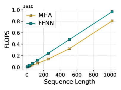
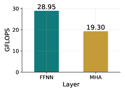
Although Equations 10 and 13 show the computational cost of mha increases quadratically, it uses fewer flops when the sequence length is small compared to the ffnn. Figure 1 illustrates the growth of the number of flops of both layers when sequences’ lengths range between $100$ and $1024$ using the above formulae. Such range is the maximal range for many language models used to solve SE tasks. This is further demonstrated empirically when measuring the number of flops performed by both of these layers in CodeBert [38] using the test set of the Devign [39] dataset. Thus, a potential way to reduce such complexity is to reduce the length of the sequence before feeding it to the ffnn layer.

Figure 1: Comparison between the floating points operations measured in gflops (10⁹ flops) performed by the mha and ffnn layers during one forward pass. Left: Theoretical flops count for each layer in one Transformer layer with respect to the sequence length using Equations 10 and 13. Right: Empirical flops count across all 12 layers of CodeBert on the test set of the Devign dataset.

III Approach

Figure 2: Overview of a Transformer encoder-based model using Alpine. Tokens that are highlighted in yellow represent special tokens such as [CLS] and [SEP]. Whenever applicable, we include the tensors dimensions for better clarity. In the figure, $B$ refers to the batch size, $S$ is the sequence length, and $dim$ is the hidden dimension of the model. The number of tokens that are pruned is $k$ which would differ from one layer to another.

Next, we present the pruning procedure adopted in this study in each Transformer layer and elaborate on the design choices.

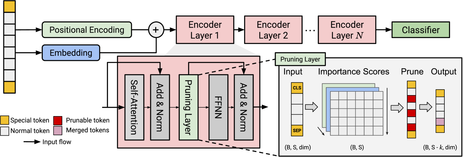
As shown in Figure 2 and Algorithm 2, the pruning layer is inserted between the mha and ffnn layers. As highlighted in Figure 1, the feed-forward layer represents a bottleneck in terms of computational costs and memory consumption [40] caused by the projection of the attention layer’s output to a higher dimension in the ffnn. Hence, performing pruning before this layer would reduce the effect of such a bottleneck.

Algorithm 1 presents the steps to perform the pruning. The first step is to assign a score to each token to determine its importance within the sequence. In this work, we use attention based scoring [28], which quantifies this importance using the attention probabilities output by the mha layer. Specifically, in L4-11 we take the mean across the attention matrices of the attention heads of the mha layer and then perform a column-wise mean to get a distribution of importance scores as illustrated by Equation 14, where $h$ is the number of attention heads, $\mathbf{A}$ is the attention matrix of an attention head and $n$ is the list of tokens excluding the special tokens [CLS], [SEP], and [PAD].

$$s(t_{i})=\frac{1}{h\cdot n}\sum_{j=1}^{h}\sum_{k=1}^{n}\mathbf{A}_{jki}$$ (14)

Algorithm 1 Perform pruning by updating the tokens mask

1:

2:$A$: Attention probabilities of each attention head.

3:$M$: Initial mask of a sequence $L$.

4:$\alpha$: Width of the bounds used for pruning tokens.

5:$M^{U}$: Updated update mask for prunable tokens.

6:$A\leftarrow\texttt{mean}(A)$ $\triangleright$ Take the mean across all attention heads

7:$scores\leftarrow\texttt{mean}(A)$ $\triangleright$ Take the mean across the columns

8:$sep\_idx\leftarrow\texttt{sum}(M)-1$ $\triangleright$ Get the index of the SEP token

9:$scores[0]\leftarrow\mathtt{NaN}$ $\triangleright$ Set CLS to NaN

10:$scores[sep\_idx]\leftarrow\mathtt{NaN}$ $\triangleright$ Set SEP to NaN

11:$seq\_len\leftarrow\texttt{length}(M)$

12:$pad\_idx\leftarrow sep\_idx+1$

13:$scores[pad\_idx:seq\_len-1]\leftarrow\mathtt{NaN}$ $\triangleright$ Set PAD to NaN

14:$\mu\leftarrow\texttt{meannan}(scores)$ $\triangleright$ Calculates the mean ignoring NaNs

15:$\sigma\leftarrow\texttt{stdnan}(scores)$ $\triangleright$ Calculates the SD ignoring NaNs

16:$max\leftarrow\mu+\alpha\cdot\sigma$

17:$min\leftarrow\mu-\alpha\cdot\sigma$

18:$keep\_tokens\leftarrow(scores\geq min)\wedge(scores\leq max)\wedge(\neg\texttt{isnan}(scores))$

19:$M^{U}\leftarrow\texttt{zeros}(\texttt{shape}(M))$ $\triangleright$ Initalize the updated mask with zeros

20:$M^{U}[keep\_tokens]\leftarrow 1$

21:$M^{U}[0]\leftarrow 1$ $\triangleright$ Set CLS to 1

22:$M^{U}[sep\_idx]\leftarrow 1$ $\triangleright$ Set SEP to 1

23:return $M^{U}$

The reason we exclude the [CLS] and [SEP] tokens from pruning is two-fold. First, the [CLS] token representation is extracted from the output of the final transformer encoder layer and fed into a linear classification layer as done previously [20, 41] Hence, such a token should be kept throughout the encoder pipeline. Second, it has been shown that these two tokens usually receive the highest attention scores [42, 25, 26] in natural and programming languages, which would skew the importance scores distribution. As for the padding token, its attention score is 0, which again would affect the score distribution, especially for shorter sequences.

Algorithm 2 Modified Transformer Encoder Layer

1:

2:Input: Input from the previous layer.

3:$M$: Input mask.

4:$\alpha$: Width of the bounds used for pruning tokens.

5:$merge$: A boolean indicating whether pruned tokens should be merged.

6:output^FFNN: Output of the FFNN layer to the subsequent layer.

7:$M^{U}$: Input mask for the subsequent layer.

8:output^MHA, $A$ $\leftarrow$ MHA(Input, $M$)

9:output^MHA $\leftarrow$ LayerNorm(Input + output^MHA)

10:$M^{U}$ $\leftarrow$ Prune($A$, $M$, $\alpha$)

11:output^MHA, $M^{U}$ $\leftarrow$ RepackTensor(output^MHA, $M^{U}$, $merge$)

12:output^FFNN $\leftarrow$ FFNN(output^MHA)

13:output^FFNN $\leftarrow$ LayerNorm(output^FFNN + output^MHA)

14:return output^FFNN, $M^{U}$

Once we obtain the importance scores distribution, we keep the tokens that are within a specific range. We set the range to be $R=[\mu-\alpha\cdot\sigma\;,\;\mu+\alpha\cdot\sigma]$, where $\mu$ and $\sigma$ are the mean and standard deviation of the importance scores distribution, and $\alpha$ is a hyperparameter that defines the width of the lower and upper bounds as shown in L12-16. The smaller $\alpha$ gets, the tighter the window, the less tokens are kept. This hyperparameter controls the aggressiveness of pruning.

Given the importance scores and the range $R$, we create a new mask $M^{U}$ that indicates the tokens that should be pruned and those that should be kept (L17-20),

$$M^{U}[i]=\begin{cases}0&\text{if }t_{i}=\text{{{[PAD]}}{}}\text{ or }s(t_{i})\notin R,\\ 1&\text{otherwise.}\end{cases}$$

Algorithm 2 shows the modified implementation of the Transformer layer. The highlighted lines L7 and L8 represent the modification that we have introduced. This also demonstrates the ease of integrating Alpine with minimal effort.

Using the updated mask from the previous step, we remove the rows from the mha output matrix that correspond to the tokens to be pruned as shown in L8. In an alternative experiment setting, we merge the rows identified for pruning into one row rather than completely removing them. Our reason is to minimize the information loss incurred by pruning. Next, the matrix’s dimensions are reduced. We also calculate the final mask since this operation is performed on a batch of sequences to guarantee that all sequences are of equal length.

We also experiment with three variants of pruning. The first one involves performing pruning across all layers of the encoder. In the second setting, it is performed only for even-indexed layers (i.e., $0,2,4,6,8,10$). Whereas the final one involves pruning at odd-indexed layers (i.e., $1,3,5,7,9,11$).

IV Experiments

The goal of this study is to investigate the effect of Alpine on language models of code when applied to SE tasks. The research aims to assess the balance between efficiency, from computational and environmental points of view, and model accuracy. Toward this goal, we formulate the following research questions. The rest of the section elaborates on the experiments designed to answer the research questions.

• To what extent does pruning on language models for code save computational resources?
  Intuitively, the less data a model processes, the more computation is saved. With this question, we wish to confirm and quantify these computational savings compared to the baseline, non-pruned model.

• What is the impact of the pruning technique on the performance of language models for code on various SE tasks?
  Naturally, pruning tokens would result in some information loss. Through this research question, we aim to measure the extent of performance drop, in terms of accuracy, for example, that might occur, if any.

• What is the effect of merging prunable tokens as opposed to completely dropping them?
  The proposed approach allows to choose whether tokens that are pruned to be partially kept by merging their representation into a single row or to be entirely removed from the sequence. In this research question, we investigate the impact of such a design choice.

• What is the impact of the computing environment on the efficiency of the pruning method?
  Finally, an important reason behind model simplification is to allow computationally demanding models to run on relatively lesser-capable gpus (e.g., consumer-grade gpus) compared to those used in high-performance computing clusters (e.g., NVIDIA V$100$ or A$100$). This exploration would ensure wider accessibility and would make the usage of these models more practical.

IV-A Model selection

The key selection criterion for the models is that they should be encoder-only Transformer-based language models for code that is publicly available. Based on the criteria, we identify the following models for our experiments.

CodeBERT [38]: It is a pre-trained language model that has the same architecture and a similar pretraining strategy as RoBERTa [43]. It comprises twelve Transformer layers, each containing a 12-headed mha layer and has a hidden dimension of $768$. It was trained on bimodal data consisting of pairs of natural language and programming language across six programming languages from the CodeSearchNet dataset [44].

GraphCodeBERT [45]: GraphCodeBert extends CodeBert by including the data flow information within the source code input. It also includes an additional pre-training task where the objective is to predict whether a data flow edge exists between two nodes.

UniXCoder [31]: UniXCoder leverages a multi-modal input consisting of natural language, source code, and the flattened sequence of the abstract syntax tree of the code snippet. It is similar to the two other models that share the same internal architecture. The difference here (aside from the pre-training objectives and input representation during pre-training) is that UniXCoder allows for a larger context length, $1024$ compared to $512$ for (Graph)CodeBERT.

IV-B Software Engineering Tasks

In this study, we choose two substantially different tasks from the CodeXGLUE benchmark [41] for our experiments.

Code clone detection: This task is taken from the filtered version of the BigCloneBenchmark dataset [46] released by Wang et al. [47]. This binary classification problem aims to predict whether two Java code snippets are clones. The dataset is composed of $901K$ training pairs and $415K$ pairs for testing. We randomly take a subsample of $90K$ pairs for training and $4K$ for evaluation; such random sampling is quite common in this domain [20, 48]. We use the same subsamples for all experiments during training and evaluation.

Defect prediction: Zhou et al. [39] proposed this dataset from a set of four large-scale open-source C repositories. The authors manually annotated the code snippets and covered multiple types of defects such as resource leaks and use-after-free vulnerabilities. We use the default pre-split sets of $21,854$ samples for training and $2,732$ for validation and testing.

We use the same model architecture in both tasks. Specifically, we add a classifier in the form of a dense layer on top of each encoder. It takes as input the last hidden representation of the [CLS] token.

IV-C Evaluation Metrics

To assess the predictive performance of the models on the aforementioned tasks, we use the same evaluation metrics that were reported by Lu et al. [41] in the CodeXGLUE benchmark. Specifically, we calculate the accuracy for the Devign dataset and F1-score for the BigCloneBenchmark. As for the computational efficiency, we report the number of floating points operations (flops) and Throughput. As stated in Section II-C the number flops quantifies the computational complexity. A model with a higher flop count requires more computing resources. Our goal here is to reduce such a count while maintaining the predictive performance as much as possible. The throughput refers to the number of input samples a model can process in a second. This metric is especially relevant during inference and model deployment.

IV-D Experimental Setting

We ran the experiments on two machines. The first machine has an amd Milan 7413 cpu, $64$gb of ram and an NVIDIA A$100$ with $40$gb of vram. The second machine has an Intel i$7-8700$ cpu, $32$gb of ram, and an NVIDIA RTX$2080$ gpu with $8$gb of vram. We use the same hyperparameters set in the CodeXGLUE benchmark for each task.

TABLE II: Comparison of the pruning method for two SE tasks using three language models. The highest accuracy or F1-score is underlined and bolded. The pruning method with the highest accuracy is highlighted with a $\bigstar$. In the FLOPs column, the values between parenthesis indicate the speedup ratio achieved by the pruning setting compared to the non-pruned model. The unit of throughput (TP) is samples per second and the reported values were measured on an NVIDIA RTX$2080$.

CodeBert				GraphCodeBert			UniXCoder
Pruning Method	Accuracy	FLOPs ($\times 10^{9}$)	TP	Accuracy	FLOPs ($\times 10^{9}$)	TP	Accuracy	FLOPs ($\times 10^{9}$)	TP
No Pruning	$64.02$%	$48.29$	$69.34$	$\mathbf{\underline{64.7}}$%	$48.29$	$69.19$	$\mathbf{\underline{66.54}}$%	$48.29$	$69.37$
All Layers	$62.3$%	$20.97\,(\times 2.3)$	$98.03$	$61.49$%	$23.84\,(\times 2.02)$	$91.29$	$65.44$%	$27.45\,(\times 1.75)$	$81.61$
Even Indexed $L=0,2,\dots 10$	$64.09$%	$33.25\,(\times 1.44)$	$81.75$	$64.02$%$\bigstar$	$34.51\,(\times 1.39)$	$80.07$	$65.62$%$\bigstar$	$37.003\,(\times 1.3)$	$74.73$
Odd Indexed $L=1,3,\dots 11$	$\mathbf{\underline{64.68}}$%$\bigstar$	$36.59\,(\times 1.31)$	$74.22$	$63.79$%	$36.66\,(\times 1.31)$	$74.93$	$65.59$%	$39.01\,(\times 1.23)$	$72.03$

(a) Defect Prediction (Devign)

CodeBert				GraphCodeBert			UniXCoder
Pruning Method	F1	FLOPS ($\times 10^{9}$)	TP	F1	FLOPS ($\times 10^{9}$)	TP	F1	FLOPS ($\times 10^{9}$)	TP
No Pruning	$\mathbf{\underline{93.09}}$%	$96.6$	$34.12$	$91.98$%	$96.5$	$33.85$	$95.07$%	$96.5$	$34.22$
All Layers	$90.57$%	$48.2\,(\times 2)$	$51.71$	$90.74$%	$47.5\,(\times 2.03)$	$51.54$	$94.7$%	$57.7\,(\times 1.67)$	$47.21$
Even Indexed $L=0,2,\dots 10$	$90.39$%	$65.7\,(\times 1.47)$	$44.88$	$\mathbf{\underline{92.13}}$%$\bigstar$	$68.5\,(\times 1.40)$	$43.10$	$94.5$%	$80.4\,(\times 1.2)$	$36.32$
Odd Indexed $L=1,3,\dots 11$	$92.17$%$\bigstar$	$68.5\,(\times 1.41)$	$42.23$	$91.46$%	$73.9\,(\times 1.30)$	$39.05$	$\mathbf{\underline{95.47}}$%$\bigstar$	$81.5\,(\times 1.18)$	$35.87$

(b) Code Clone Detection (BigCloneBenchmark)

(a) Defect Prediction (Devign)

(b) Code Clone Detection (BigCloneBenchmark)

Figure 3: The progressive average reduction in sequences’ lengths as the input traverses through the layers of each model. The plots are the result of a forward pass across the whole test set of each dataset with a batch size of 8.

V Results

V-A RQ1: Computational Efficiency

TABLE III: The effect of token merging on models’ accuracy and F1-scores. w/ m refers to the setting where token merging is enabled whereas w/o m indicates pruning without merging. As a reminder the performance metric for defect prediction is accuracy and F1 for code clone detection.

Model

Task

Defect Prediction

Code Clone Detection

All

Even

Odd

All

Even

Odd

w/ m

w/o m

w/ m

w/o m

w/ m

w/o m

w/ m

w/o m

w/ m

w/o m

w/ m

w/o m

CodeBert

$\mathbf{62.3}$%

$61.8$%

$\mathbf{64.09}$%

$63.7$%

$\mathbf{64.68}$%

$64.09$%

$\mathbf{90.57}$%

$89.63$%

$\mathbf{90.39}$%

$90.30$%

$\mathbf{92.17}$%

$91.06$%

GraphCodeBert

$\mathbf{61.49}$%

$61.05$%

$\mathbf{64.02}$%

$62.2$%

$\mathbf{63.79}$%

$62.66$%

$\mathbf{90.74}$%

$90.71$%

$\mathbf{92.13}$%

$91.63$%

$\mathbf{91.46}$%

$91.06$%

UniXCoder

$\mathbf{65.44}$%

$64.20$%

$\mathbf{65.62}$%

$64.49$%

$\mathbf{65.59}$%

$65.52$%

$\mathbf{94.7}$%

$93.64$%

$\mathbf{94.5}$%

$93.62$%

$\mathbf{95.47}$%

$94.4$%

Impact on FLOPs Count: Table II(b) highlights the computational speedup offered by Alpine across the three models on the SE tasks. Performing pruning across all layers allows for the most computational savings. On average, it reduces the flops count by $\times 2.01$ on the Devign dataset and $\times 1.9$ and BigCloneBenchmark compared the baseline models (i.e., without any pruning). Specifically, CodeBert and GraphCodeBert exhibit roughly the same gain, where these models consume roughly half flops. UniXCoder also show significant gain, though slightly smaller ($\times 1.67$ and $\times 1.75$), in terms of flops.

Interestingly, performing pruning at even indexed layers seems to yield lower operations compared to pruning at odd indexed layers. A possible explanation for this behavior is that there is a considerable drop in the number of tokens at the 0^th layer which would have an earlier cascading effect if we were to perform this at a later layer.

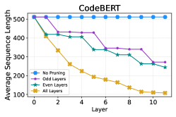
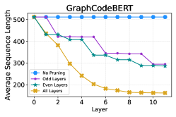
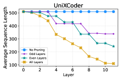
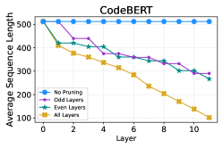
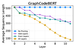
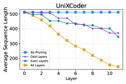
In Figure 3, we plot the average sequence length across all the twelve layers during inference. When pruning across all layers on the Devign dataset, the sequence length plot exhibits an exponential-like decay on CodeBert and GraphCodeBert. On the other hand, this reduction follows roughly a linear trend on BigCloneBenchmark across all models. What is interesting is that at the final layer, the sequences are quite compressed. Specifically, the highest average sequence length at the last layer ($162$) is obtained when using GraphCodeBert on the defect prediction task which is $\sim\times 3$ less than the none pruned average length of $512$. In addition, aligned with the results of Table II(b), we can see that pruning at even-indexed layers yields shorter sequences than odd-indexed ones. Across all task-model combinations and all layers (except for $2$-$4$ layer), Alpine produces more compressed sequences when applied at these layers compared to their odd-indexed counterpart.

Impact on Throughput: Pruning across all layers consistently yields the highest throughput improvement for all models and tasks. For instance, CodeBert’s throughput increases from $69.34$ to $98.03$ ($41.4$% improvement) for the defect prediction task and from $34.12$ to $51.71$ ($51.6$% improvement) for code clone detection. Moreover, applying pruning in even-indexed layers generally results in better throughput compared to pruning odd-indexed layers. This trend is evident across all models and tasks, with even-indexed layer pruning providing an average throughput improvement of $16.7$% compared to no pruning, while odd-indexed layer pruning offers an average improvement of $9.3$%.

Another observation is that the extent of improvement varies among the models. GraphCodeBert exhibits the highest average throughput improvement of $30.8$% across all pruning methods and tasks, followed by CodeBert with $28.5$% and UniXCoder with $20.1$%. In general, the models achieved higher throughput on the Devign dataset, regardless of the pruning method applied. The average throughput for this task is $79.4$ samples per second, while for the code clone detection task, it is $41.5$ samples per second.

The increase in throughput is attributed to Alpine’s ability to compress sequences. A smaller sequence length allows for more efficient parallel processing and reduces the computational overhead associated with longer sequences, resulting in higher throughput and faster processing times.

Impact on Memory Footprint: To further evaluate Alpine’s impact from a computational efficiency standpoint, we plot the gpu memory consumption. Due to space constraints, we only report the figures regarding pruning across all layers.

Figure 4: Comparison of the gpu memory footprint between the pruned and non-pruned models across the tasks.

From the plot in Figure 4, we see that Alpine significantly reduces memory consumption across all models and tasks. CodeBert exhibits the highest percentage of memory reduction for the defect detection task ($72$%), while GraphCodeBert and UniXCoder show more consistent reductions across both tasks ($56.7$% to $66.7$%).

This reduction leads to improved cost efficiency, faster data transfer, and power efficiency. By requiring less memory, models can be deployed on more affordable gpus with smaller memory capacities, reducing hardware costs. Additionally, a smaller memory footprint results in faster data transfer between the cpu and gpu; the additional speed, in turn, increases throughput as demonstrated earlier. Moreover, minimizing the model’s memory footprint contributes to reduced power consumption, which is crucial in constrained environments.

V-B RQ2: Impact on Performance

In Table II(b), we report the predictive performance of the pruned models. On the Devign dataset, performing pruning at odd-indexed layers leads to a slight improvement when using CodeBert, with a $0.66$% increase in accuracy compared to that of the non-pruned version. On the other hand, adding the pruning layer at even layers is more efficient for GraphCodeBert and UniXCoder, where they were able to maintain $98.94$% and $98.61$% of the original accuracy scores, respectively.

In the clone detection task, pruning at even-indexed layers achieves the highest F1-scores compared to other pruning strategies. It even managed to improve the clone detection performance by increasing the F1-scores of GraphCodeBert and UniXCoder by $0.15$% and $0.4$%.

Applying Alpine at all layers not only leads to $\times 2$ less computation but also results in a high level of predictive performance for all three models. UniXCoder exhibits the highest performance both before and after pruning, retaining $98.3$% of its original accuracy. CodeBert and GraphCodeBert also demonstrate strong performance retention, preserving $97.3$% and $94.4$% of their original accuracy, respectively. A similar observation can also be made for the results of code clone detection. All models maintain a high level of performance after pruning, with UniXCoder achieving the highest F1-score retention at $99.6$% of its original score. GraphCodeBert and CodeBert also demonstrate strong performance, retaining $98.7$% and $97.3$% of their original F1-scores, respectively.

Among the three models, UniXCoder shows the highest resilience to pruning, keeping an average of $99$% of its original performance across both tasks and all pruning methods.

V-C RQ3: Effect of Merging Prunable Tokens on Model Accuracy

During pruning, the representation of tokens marked to be pruned can be entirely removed or merged into one vector. To study the impact of token merging, we conduct experiments to measure its impact on the two tasks and report the results in Table III.

Across all models and datasets, merging tokens consistently yields better performance compared to discarding them completely. UniXCoder benefits the most from this design choice, with an average performance improvement of $1.14$% on Devign and $1$% on BigCloneBenchmark.

On the Devign dataset, GraphCodeBert shows the highest performance gain when pruning even layers ($1.82$%), while CodeBert’s performance is enhanced the most when pruning odd layers on the BCB dataset ($1.11$%). In contrast, GraphCodeBert exhibits the least improvement when pruning all layers on the BigCloneBenchmark dataset ($0.03$%).

V-D RQ4: Impact of Computing Environment

In Figures 5 and 6, we plot the time taken to fine-tune the language models on the selected tasks when using different gpus. First, examining the results for the A$100$ gpu, we observe that Alpine leads to a reduction in fine-tuning time for all three models on both the tasks. For defect prediction, pruning results in a running time reduction of around $25$% for CodeBert, $24$% for GraphCodeBert, and 15% for UniXCoder. Similarly, for the clone detection task, pruning reduces the running time by approximately $18$% for CodeBert, $11$% for GraphCodeBert, and $12$% for UniXCoder. These findings demonstrate that pruning is effective in improving the efficiency of the models on a high-performance gpu.

Figure 5: Fine-tuning time before and after pruning on an NVIDIA A100 gpu.

Next, comparing the results between the RTX$2080$ and A$100$ gpus, we notice that the running times on the A$100$ are generally shorter than those on the RTX$2080$, both with and without pruning. This is expected due to the superior computational capabilities of the A$100$. However, the relative impact of pruning on efficiency differs between the two gpus. On the RTX$2080$, pruning leads to a more significant reduction in running time, with improvements ranging from $39$% to $54$% across models and tasks. In contrast, on the A$100$, the reduction in running time due to pruning is less pronounced, ranging from $11$% to $25$%.

Figure 6: Fine-tuning time before and after pruning on an NVIDIA RTX2080 gpu.

Building upon these results, we further investigate the implications of the reduced time from an environmental perspective. In Table IV, we report the CO₂ emission rates for both gpus with and without Alpine. The measurements were taken using the tool provided by Lacoste et al. [18].

TABLE IV: gpu emission statistics across two NVIDIA gpus.

gpu	E(CO2 kg) without Alpine	E(CO2 kg) with Alpine	Emission reduction rate
RTX$2080$	$5.93$	$0.34$	$44.85$%
A$100$	$3.15$	$2.69$	$14.60$%

The results show that Alpine significantly reduces the CO₂ emissions of both the RTX$2080$ and A$100$ gpus. For the RTX$2080$, the amount of CO₂ emitted decreases from $5.93$ kg to $0.34$ kg with Alpine, resulting in a substantial emission reduction rate of $44.85$%. Similarly, for the A$100$, emissions decrease from $3.15$ kg to $2.69$ kg, resulting in a reduction rate of $14.60$%. The reduction in emissions is particularly significant for the RTX$2080$, which aligns with the previous analysis showing that pruning leads to a more substantial improvement in efficiency on consumer-grade gpus compared to high-performance gpus like the A$100$.

VI Threats to Validity

Internal validity: Internal threats to validity are concerned with the ability to draw conclusions from our experimental results. The hyperparameters specified for a model influence the time, resources required, and the results. To mitigate a potential threat, we used the same hyperparameters across all models, as reported in previous works [41], and utilized the same data splits for fine-tuning and testing. This consistency in the experimental setup strengthens the internal validity of our findings, ensuring that the observed effects can be attributed to the Alpine pruning method rather than variations in hyperparameters or data splits.
External validity: External threats to validity are concerned with the ability to generalize our results. The language-agnostic nature of the Alpine pruning method allows it to be applied to a wide range of programming languages without the need for language-specific adaptations. We evaluate the approach on three language models and tasks with different programming languages (C and Java). Its compatibility with all transformer-based encoder models makes it easily integrable into various architectures, enhancing its generalization. Finally, the two gpus used in this study, NVIDIA A$100$ and RTX$2080$, belong to Ampere and Turning architecture families. These architectures encompass a larger set of other cards which we expect to exhibit the similar reported trends.
Construct validity: Construct threats to validity are concerned with the degree to which our analyses measure what we claim to analyze. We employed well-established metrics for measuring predictive performance (such as, accuracy and F1-score), computational efficiency (flops, throughput, running time and memory footprint), and environmental impact through CO₂ emissions rate. Relying on the traditional metrics for the measured aspects mitigates the potential threats of construct validity and ensures that the variables are accurately captured.

VII Related Work

VII-A Pre-trained language models of code

Pre-trained code language models have demonstrated benefits in various SE tasks, including code search, code and documentation generation, and defect prediction [32, 31, 41, 49]. Typically based on the transformer architecture [1], these models can broadly be categorized into decoder-only, encoder-only, and encoder-decoder language models [50].

Decoder-only architectures are typically pre-trained in an autoregressive manner, i.e., predicting the subsequent token based on preceding ones. In the realm of code, examples include InCoder [33], StarCoder 2 [35], and CodeGen 2 [51]. These architectures excel in code generation tasks.

Encoder-only architectures are primarily pre-trained on the masked language modeling task i.e., these models are trained to predict masked words given the remaining sequence as context. Examples include CodeBert [38] and GraphCodeBert [45]. They are frequently used for classification tasks or as a means of feature extraction.

Encoder-decoder architectures undergo pre-training through conditional generation tasks i.e., generating text based on provided input text, e.g., for code summarization or generating code from natural language descriptions. Sample architectures include CodeT5 [32], CodeT5+[52], and plbart [53].

While the experiments in the paper primarily focus on encoder-only models (i.e., CodeBert, GraphCodeBert, and UniXCoder), the proposed pruning layer can be used in both decoder-only and encoder-only architectures. Further experimentation is needed to determine if such layer is also effective in those architectures which is left as future work.

VII-B Optimized transformers

The techniques to enhance the effectiveness of a given transformer model while maintaining its performance fall into three categories—knowledge distillation, quantization, and pruning [20, 28, 54].

Knowledge distillation. The main idea of this technique is to train a smaller model (the student model) to imitate the behavior of a larger model (the teacher model) [55]. In a SE context, Shi et al. [20] introduced Compressor, a framework that employs task-specific knowledge distillation to improve the efficiency of the final transformer model. The authors perform a neural architectural search via a genetic algorithm, followed by training the selected model using knowledge distillation. In their experiments, they use CodeBert [38] and GraphCodeBert [45] as teacher models to tackle the tasks of vulnerability prediction and code clone detection. Compressor still requires the fine-tuning of the teacher model, which incurs overhead throughout the process. Alpine allows to reduce the computational costs of fine-tuning these models, which entails, that such overhead can be reduced.

Quantization. Quantization aims to reduce the memory footprint of neural networks. The core idea is to convert the model’s parameters from 32-bit floating-point numbers (float32 data type) to lower-precision formats, such as 8-bit integers (int8 data type) [56]. Depending on the component of quantization, these techniques can be categorized as quantization of weights only [57, 58, 59] and quantization of both weights and activations [60, 61, 62]. Although quantization reduces the memory footprint of these models, it may also reduce the inference speed and accuracy [63].

Pruning. As mentioned previously, pruning techniques can be divided into weight pruning and token pruning [28]. Liu et al.[64] adopt weight pruning to prune unimportant heads and channels from the mha and ffnn respectively. Zang et al. [22] offer DietCode—a token pruning approach. To build DietCode, Zang et al. carry out an empirical investigation to determine the significance of statements and tokens for CodeBert. Subsequently, based on these findings, they employ a 0-1 Knapsack approach to prune the input sequence. In contrast, our approach is performed adaptively at each layer. Additionally, during the pruning step, we could aggregate the pruned tokens into a single one to prevent excessive loss of information. Finally, our method is language-agnostic, facilitating easy adaptation to diverse programming languages and extending applicability to natural language inputs, particularly beneficial in minimizing computational overhead in tasks like code search or code generation from documentation.

VIII Conclusions and Future Work

This study addresses the challenges, specifically computational efficiency and environmental impact, associated with language models of code. We propose Alpine, a pruning method that reduces the input sequence while maintaining predictive performance. Our experiments on three language models and datasets with different programming languages demonstrate that it significantly improves computational efficiency that, in turn, reduces CO₂ emissions. The results show that it is particularly effective on consumer-grade gpus, enabling the usage of these models on more accessible hardware. Furthermore, the programming language-agnostic nature of Alpine and its compatibility with Transformer-based models enhance the generalizability of our findings. We envision to extend this work along two axes. First, we aim to assess Alpine on bigger models with parameter count $>$ 1Bn, and across different Transformers variants, i.e.,, the encoder-decoder, and the decoder models. The second dimension relates to making Alpine even more adaptive and customizable by introducing different importance scoring functions.

References

- [1] A. Vaswani, N. Shazeer, N. Parmar, J. Uszkoreit, L. Jones, A. N. Gomez, L. u. Kaiser, and I. Polosukhin, “Attention is all you need,” in Advances in Neural Information Processing Systems, vol. 30, 2017.
- [2] A. Hindle, E. T. Barr, Z. Su, M. Gabel, and P. Devanbu, “On the naturalness of software,” in Proceedings of the 34th International Conference on Software Engineering, ICSE ’12, 2012.
- [3] Y. Lai, C. Li, Y. Wang, T. Zhang, R. Zhong, L. Zettlemoyer, W.-t. Yih, D. Fried, S. Wang, and T. Yu, “Ds-1000: A natural and reliable benchmark for data science code generation,” in International Conference on Machine Learning, pp. 18319–18345, PMLR, 2023.
- [4] Z. Zeng, H. Tan, H. Zhang, J. Li, Y. Zhang, and L. Zhang, “An extensive study on pre-trained models for program understanding and generation,” in Proceedings of the 31st ACM SIGSOFT International Symposium on Software Testing and Analysis, ISSTA 2022, p. 39–51, 2022.
- [5] V. Dibia, A. Fourney, G. Bansal, F. Poursabzi-Sangdeh, H. Liu, and S. Amershi, “Aligning offline metrics and human judgments of value for code generation models,” in Findings of the Association for Computational Linguistics: ACL 2023 (A. Rogers, J. Boyd-Graber, and N. Okazaki, eds.).
- [6] F. Chen, F. H. Fard, D. Lo, and T. Bryksin, “On the transferability of pre-trained language models for low-resource programming languages,” in Proceedings of the 30th IEEE/ACM International Conference on Program Comprehension, ICPC ’22, p. 401–412, 2022.
- [7] M. Alqarni and A. Azim, “Low Level Source Code Vulnerability Detection Using Advanced BERT Language Model,” Proceedings of the Canadian Conference on Artificial Intelligence, may 27 2022.
- [8] A. Ciborowska and K. Damevski, “Too few bug reports? exploring data augmentation for improved changeset-based bug localization,” arXiv preprint arXiv:2305.16430, 2023.
- [9] S. Fatima, T. A. Ghaleb, and L. Briand, “Flakify: A black-box, language model-based predictor for flaky tests,” IEEE Transactions on Software Engineering, vol. 49, no. 4, pp. 1912–1927, 2023.
- [10] W. Tang, M. Tang, M. Ban, Z. Zhao, and M. Feng, “Csgvd: A deep learning approach combining sequence and graph embedding for source code vulnerability detection,” J. Syst. Softw., may 2023.
- [11] H. Tian, K. Liu, Y. Li, A. K. Kaboré, A. Koyuncu, A. Habib, L. Li, J. Wen, J. Klein, and T. F. Bissyandé, “The best of both worlds: Combining learned embeddings with engineered features for accurate prediction of correct patches,” ACM Trans. Softw. Eng. Methodol., 2023.
- [12] Q. Zhang, C. Fang, W. Sun, Y. Liu, T. He, X. Hao, and Z. Chen, “Boosting automated patch correctness prediction via pre-trained language model,” 2023.
- [13] T. Le-Cong, D.-M. Luong, X. B. D. Le, D. Lo, N.-H. Tran, B. Quang-Huy, and Q.-T. Huynh, “Invalidator: Automated patch correctness assessment via semantic and syntactic reasoning,” IEEE Transactions on Software Engineering, 2023.
- [14] R. Paul, M. M. Hossain, M. Hasan, and A. Iqbal, “Automated program repair based on code review: How do pre-trained transformer models perform?,” arXiv preprint arXiv:2304.07840, 2023.
- [15] A. Moharil and A. Sharma, “Tabasco: A transformer based contextualization toolkit,” Science of Computer Programming, 2023.
- [16] S. Ezzini, S. Abualhaija, C. Arora, and M. Sabetzadeh, “Automated handling of anaphoric ambiguity in requirements: a multi-solution study,” in Proceedings of the 44th International Conference on Software Engineering.
- [17] A. S. Luccioni, Y. Jernite, and E. Strubell, “Power hungry processing: Watts driving the cost of ai deployment?,” arXiv preprint arXiv:2311.16863, 2023.
- [18] A. Lacoste, A. Luccioni, V. Schmidt, and T. Dandres, “Quantifying the carbon emissions of machine learning,” arXiv preprint arXiv:1910.09700, 2019.
- [19] X. Wang, C. Na, E. Strubell, S. Friedler, and S. Luccioni, “Energy and carbon considerations of fine-tuning BERT,” in Findings of the Association for Computational Linguistics: EMNLP 2023, Association for Computational Linguistics, Dec. 2023.
- [20] J. Shi, Z. Yang, B. Xu, H. J. Kang, and D. Lo, “Compressing pre-trained models of code into 3 mb,” in Proceedings of the 37th IEEE/ACM International Conference on Automated Software Engineering, ASE ’22, (New York, NY, USA), Association for Computing Machinery, 2023.
- [21] G. E. Hinton, O. Vinyals, and J. Dean, “Distilling the knowledge in a neural network,” ArXiv, vol. abs/1503.02531, 2015.
- [22] Z. Zhang, H. Zhang, B. Shen, and X. Gu, “Diet code is healthy: simplifying programs for pre-trained models of code,” in Proceedings of the 30th ACM Joint European Software Engineering Conference and Symposium on the Foundations of Software Engineering, ESEC/FSE 2022, 2022.
- [23] Anonymous, “Alpine replication package.” https://anonymous.4open.science/r/ICSE25-Alpine-Replication-Package-F82D/README.md.
- [24] X. Hou, Y. Zhao, Y. Liu, Z. Yang, K. Wang, L. Li, X. Luo, D. Lo, J. C. Grundy, and H. Wang, “Large language models for software engineering: A systematic literature review,” ArXiv, vol. abs/2308.10620, 2023.
- [25] G. Kobayashi, T. Kuribayashi, S. Yokoi, and K. Inui, “Attention is not only a weight: Analyzing transformers with vector norms,” 2020.
- [26] M. Saad and T. Sharma, “Naturalness of attention: Revisiting attention in code language models,” 2023.
- [27] T. Liang, J. Glossner, L. Wang, S. Shi, and X. Zhang, “Pruning and quantization for deep neural network acceleration: A survey,” Neurocomputing, vol. 461, pp. 370–403, 2021.
- [28] S. Kim, S. Shen, D. Thorsley, A. Gholami, W. Kwon, J. Hassoun, and K. Keutzer, “Learned token pruning for transformers,” in Proceedings of the 28th ACM SIGKDD Conference on Knowledge Discovery and Data Mining, KDD ’22, (New York, NY, USA), Association for Computing Machinery, 2022.
- [29] X. Hou, Y. Zhao, Y. Liu, Z. Yang, K. Wang, L. Li, X. Luo, D. Lo, J. Grundy, and H. Wang, “Large language models for software engineering: A systematic literature review,” arXiv preprint arXiv:2308.10620, 2023.
- [30] W. X. Zhao, K. Zhou, J. Li, T. Tang, X. Wang, Y. Hou, Y. Min, B. Zhang, J. Zhang, Z. Dong, et al., “A survey of large language models,” arXiv preprint arXiv:2303.18223, 2023.
- [31] D. Guo, S. Lu, N. Duan, Y. Wang, M. Zhou, and J. Yin, “UniXcoder: Unified cross-modal pre-training for code representation,” in Proceedings of the 60th Annual Meeting of the Association for Computational Linguistics (Volume 1: Long Papers), Association for Computational Linguistics, May 2022.
- [32] Y. Wang, W. Wang, S. Joty, and S. C. Hoi, “CodeT5: Identifier-aware unified pre-trained encoder-decoder models for code understanding and generation,” in Proceedings of the 2021 Conference on Empirical Methods in Natural Language Processing, pp. 8696–8708, Association for Computational Linguistics, Nov. 2021.
- [33] D. Fried, A. Aghajanyan, J. Lin, S. Wang, E. Wallace, F. Shi, R. Zhong, S. Yih, L. Zettlemoyer, and M. Lewis, “Incoder: A generative model for code infilling and synthesis,” in The Eleventh International Conference on Learning Representations, 2023.
- [34] J. Devlin, M.-W. Chang, K. Lee, and K. Toutanova, “Bert: Pre-training of deep bidirectional transformers for language understanding,” arXiv preprint arXiv:1810.04805, 2018.
- [35] A. Lozhkov, R. Li, L. B. Allal, F. Cassano, J. Lamy-Poirier, N. Tazi, A. Tang, D. Pykhtar, J. Liu, Y. Wei, et al., “Starcoder 2 and the stack v2: The next generation,” arXiv preprint arXiv:2402.19173, 2024.
- [36] R. Hunger, Floating Point Operations in Matrix-vector Calculus. Munich University of Technology, Inst. for Circuit Theory and Signal Processing, 2005.
- [37] D. Hendrycks and K. Gimpel, “Gaussian error linear units (gelus),” arXiv preprint arXiv:1606.08415, 2016.
- [38] Z. Feng, D. Guo, D. Tang, N. Duan, X. Feng, M. Gong, L. Shou, B. Qin, T. Liu, D. Jiang, and M. Zhou, “CodeBERT: A pre-trained model for programming and natural languages,” in Findings of the Association for Computational Linguistics: EMNLP 2020, Association for Computational Linguistics, Nov. 2020.
- [39] Y. Zhou, S. Liu, J. Siow, X. Du, and Y. Liu, “Devign: Effective vulnerability identification by learning comprehensive program semantics via graph neural networks,” in Advances in Neural Information Processing Systems, pp. 10197–10207, 2019.
- [40] P. Ganesh, Y. Chen, X. Lou, M. A. Khan, Y. Yang, H. Sajjad, P. Nakov, D. Chen, and M. Winslett, “Compressing large-scale transformer-based models: A case study on BERT,” Transactions of the Association for Computational Linguistics, vol. 9, 2021.
- [41] S. Lu, D. Guo, S. Ren, J. Huang, A. Svyatkovskiy, A. Blanco, C. B. Clement, D. Drain, and other, “Codexglue: A machine learning benchmark dataset for code understanding and generation,” CoRR, vol. abs/2102.04664, 2021.
- [42] K. Clark, U. Khandelwal, O. Levy, and C. D. Manning, “What does bert look at? an analysis of bert’s attention,” 2019.
- [43] Y. Liu, M. Ott, N. Goyal, J. Du, M. Joshi, D. Chen, O. Levy, M. Lewis, L. Zettlemoyer, and V. Stoyanov, “Roberta: A robustly optimized bert pretraining approach,” arXiv preprint arXiv:1907.11692, 2019.
- [44] H. Husain, H.-H. Wu, T. Gazit, M. Allamanis, and M. Brockschmidt, “Codesearchnet challenge: Evaluating the state of semantic code search,” arXiv preprint arXiv:1909.09436, 2019.
- [45] D. Guo, S. Ren, S. Lu, Z. Feng, D. Tang, S. LIU, L. Zhou, N. Duan, A. Svyatkovskiy, S. Fu, M. Tufano, S. K. Deng, C. Clement, D. Drain, N. Sundaresan, J. Yin, D. Jiang, and M. Zhou, “Graphcode{bert}: Pre-training code representations with data flow,” in International Conference on Learning Representations, 2021.
- [46] J. Svajlenko, J. F. Islam, I. Keivanloo, C. K. Roy, and M. M. Mia, “Towards a big data curated benchmark of inter-project code clones,” in 2014 IEEE International Conference on Software Maintenance and Evolution, pp. 476–480, IEEE, 2014.
- [47] W. Wang, G. Li, B. Ma, X. Xia, and Z. Jin, “Detecting code clones with graph neural network and flow-augmented abstract syntax tree,” in 2020 IEEE 27th International Conference on Software Analysis, Evolution and Reengineering (SANER), pp. 261–271, IEEE, 2020.
- [48] Z. Yang, J. Shi, J. He, and D. Lo, “Natural attack for pre-trained models of code,” in Proceedings of the 44th International Conference on Software Engineering, ICSE ’22, (New York, NY, USA), 2022.
- [49] T. Sharma, M. Kechagia, S. Georgiou, R. Tiwari, I. Vats, H. Moazen, and F. Sarro, “A survey on machine learning techniques applied to source code,” Journal of Systems and Software, vol. 209, p. 111934, 2024.
- [50] B. Min, H. Ross, E. Sulem, A. P. B. Veyseh, T. H. Nguyen, O. Sainz, E. Agirre, I. Heintz, and D. Roth, “Recent advances in natural language processing via large pre-trained language models: A survey,” ACM Computing Surveys, vol. 56, no. 2, pp. 1–40, 2023.
- [51] E. Nijkamp, H. Hayashi, C. Xiong, S. Savarese, and Y. Zhou, “Codegen2: Lessons for training llms on programming and natural languages,” arXiv preprint arXiv:2305.02309, 2023.
- [52] Y. Wang, H. Le, A. D. Gotmare, N. D. Bui, J. Li, and S. C. Hoi, “CodeT5+: Open code large language models for code understanding and generation,” arXiv preprint arXiv:2305.07922, 2023.
- [53] W. U. Ahmad, S. Chakraborty, B. Ray, and K.-W. Chang, “Unified pre-training for program understanding and generation,” arXiv preprint arXiv:2103.06333, 2021.
- [54] X. Zhu, J. Li, Y. Liu, C. Ma, and W. Wang, “A survey on model compression for large language models,” arXiv preprint arXiv:2308.07633, 2023.
- [55] J. Gou, B. Yu, S. J. Maybank, and D. Tao, “Knowledge distillation: A survey,” International Journal of Computer Vision, vol. 129, no. 6, pp. 1789–1819, 2021.
- [56] M. Nagel, M. Fournarakis, R. A. Amjad, Y. Bondarenko, M. Van Baalen, and T. Blankevoort, “A white paper on neural network quantization,” arXiv preprint arXiv:2106.08295, 2021.
- [57] Y. Xu, L. Xie, X. Gu, X. Chen, H. Chang, H. Zhang, Z. Chen, X. ZHANG, and Q. Tian, “Qa-lora: Quantization-aware low-rank adaptation of large language models,” in The Twelfth International Conference on Learning Representations, 2023.
- [58] T. Dettmers, A. Pagnoni, A. Holtzman, and L. Zettlemoyer, “Qlora: Efficient finetuning of quantized llms,” Advances in Neural Information Processing Systems, vol. 36, 2024.
- [59] S. Kim, C. Hooper, A. Gholami, Z. Dong, X. Li, S. Shen, M. W. Mahoney, and K. Keutzer, “Squeezellm: Dense-and-sparse quantization,” arXiv preprint arXiv:2306.07629, 2023.
- [60] O. Zafrir, G. Boudoukh, P. Izsak, and M. Wasserblat, “Q8bert: Quantized 8bit bert,” in 2019 Fifth Workshop on Energy Efficient Machine Learning and Cognitive Computing-NeurIPS Edition (EMC2-NIPS), pp. 36–39, IEEE, 2019.
- [61] Z. Yao, R. Yazdani Aminabadi, M. Zhang, X. Wu, C. Li, and Y. He, “Zeroquant: Efficient and affordable post-training quantization for large-scale transformers,” Advances in Neural Information Processing Systems, vol. 35, pp. 27168–27183, 2022.
- [62] T. Dettmers, R. A. Svirschevski, V. Egiazarian, D. Kuznedelev, E. Frantar, S. Ashkboos, A. Borzunov, T. Hoefler, and D. Alistarh, “Spqr: A sparse-quantized representation for near-lossless llm weight compression,” in The Twelfth International Conference on Learning Representations, 2023.
- [63] R. Jin, J. Du, W. Huang, W. Liu, J. Luan, B. Wang, and D. Xiong, “A comprehensive evaluation of quantization strategies for large language models,” arXiv preprint arXiv:2402.16775, 2024.
- [64] Z. Liu, F. Li, G. Li, and J. Cheng, “Ebert: Efficient bert inference with dynamic structured pruning,” in Findings of the Association for Computational Linguistics: ACL-IJCNLP 2021, pp. 4814–4823, 2021.