Simultaneous System Identification and Model
Predictive Control with No Dynamic Regret

Abstract

We provide an algorithm for the simultaneous sys- tem identification and model predictive control of nonlinear systems. The algorithm has finite-time near-optimality guarantees and asymptotically converges to the optimal (non-causal) controller. Particularly, the algorithm enjoys sublinear dynamic regret, defined herein as the suboptimality against an optimal clairvoyant controller that knows how the unknown disturbances and system dynamics will adapt to its actions. The algorithm is self-supervised and applies to control-affine systems with unknown dynamics and disturbances that can be expressed in reproducing kernel Hilbert spaces [1]. Such spaces can model external disturbances and modeling errors that can even be adaptive to the system’s state and control input. For example, they can model wind and wave disturbances to aerial and marine vehicles, or inaccurate model parameters such as inertia of mechanical systems. We are motivated by the future of autonomy where robots will autonomously perform complex tasks despite real-world unknown disturbances such as wind gusts. The algorithm first generates random Fourier features that are used to approximate the unknown dynamics or disturbances. Then, it employs model predictive control based on the current learned model of the unknown dynamics (or disturbances). The model of the unknown dynamics is updated online using least squares based on the data collected while controlling the system. We validate our algorithm in both hardware experiments and physics-based simulations. The simulations include (i) a cart-pole aiming to maintain the pole upright despite inaccurate model parameters, and (ii) a quadrotor aiming to track reference trajectories despite unmodeled aerodynamic drag effects. The hardware experiments include a quadrotor aiming to track a circular trajectory despite unmodeled aerodynamic drag effects, ground effects, and wind disturbances.

I Introduction

In the future, mobile robots will automate fundamental tasks such as package delivery [2], target tracking [3], and inspection and maintenance [4]. Such tasks require accurate and efficient tracking control. But achieving accuracy and efficiency is challenging since such tasks often require the robots to operate under highly uncertain conditions, particularly, under unknown dynamics and (possibly state-dependent) disturbances. For example, they require the quadrotors to (i) pick up and carry packages of unknown weight, (ii) chase mobile targets at high speeds where the induced aerodynamic drag is hard to model, and (iii) inspect and maintain outdoor infrastructure exposed to turbulence and wind gusts.

State-of-the-art methods for control under unknown dynamics and disturbances typically rely on offline or online methods, or a mix of the two, including: robust control [5, 6, 7, 8, 9, 10]; adaptive control and disturbance compensation [11, 12, 13, 14, 15, 16, 17, 18, 19, 20]; offline learning for control [21, 22, 23, 24, 25, 26, 27]; offline learning for control with online adaption [28, 29, 30, 31, 32, 33, 34]; and online learning [35, 36, 37, 38, 39, 40, 41]. Among these, the offline learning methods require data collection for offline training, a process that can be expensive/time-consuming [42], instead of collecting data online and learning on the spot. For this reason, these methods may not also generalize to different scenarios than those used for offline learning [43, 44]. The robust control methods, given a known upper bound on the magnitude of the noise, can be conservative due to assuming worse-case disturbance realization [45, 46], instead of planning based on an accurate predictive model of the disturbance. Similarly, the adaptive control and the online learning control methods may exhibit sub-optimal performance due to only reacting to the history of observed disturbances, instead of planning based on an accurate predictive model of the disturbance [11, 12, 13, 36]. We discuss the related work in extension in Section VII.

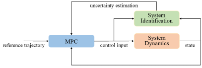
In this paper, instead, we leverage the success of model predictive control methods for accurate tracking control [47]. To this end, we propose a self-supervised method to learn online a predictive model of the unknown uncertainties (Fig. 1). Therefore, the proposed method promises to enable: one-shot online learning, instead of offline (or episodic learning); online control that adapts to the actual disturbance realization, instead of the worst-case; and control planned over a look-ahead horizon of predicted system dynamics and disturbances, instead of their past. We elaborate on our contributions next.

Figure 1: Overview of Simultaneous System Identification and Model Predictive Control Pipeline. The pipeline is composed of two interacting modules: (i) a model predictive control (MPC) module, and (ii) an online system identification module. The MPC module uses the estimated unknown disturbances/dynamics from the system identification module to calculate the next control input. Given the control input and the observed new state, the online system identification module then updates the estimate of the unknown disturbances/dynamics.

Contributions. We provide a real-time and asymptotically-optimal algorithm for the simultaneous system identification and control of nonlinear systems. Specifically, the algorithm enjoys sublinear dynamic regret, defined herein as the suboptimality against an optimal clairvoyant controller that knows how the unknown disturbances and system dynamics will adapt to its actions. The said definition of dynamic regret differs from the standard definition of dynamic regret in the literature, e.g., [36, 37, 38, 39, 40, 41] where the suboptimality of an Algorithm is measured against the controller that is optimal for the same realization of disturbances as the Algorithm experienced, instead of the realization that the optimal controller would experience given that the disturbances can be adaptive (Remark 2).

The algorithm is self-supervised and applies to control-affine systems with unknown dynamics and disturbances that can be expressed in reproducing kernel Hilbert spaces [1]. Such spaces can model external disturbances and modeling errors that are even adaptive to the system’s state and control input. For example, they can model wind and wave disturbances to aerial and marine vehicles, or inaccurate model parameters such as inertia of mechanical systems.

Description of the algorithm

The algorithm is composed of two interacting modules (Fig. 1): (i) a model predictive control (MPC) module, and (ii) an online system identification module. At each time step, the MPC module uses the estimated unknown disturbances and system dynamics from the system identification module to calculate the next control input. Given the control input and the observed new state, the online system identification module then updates the estimate of the unknown disturbances and system dynamics.

Approach of predictive online system identification

We enable the predictive online system identification module by employing online least-squares estimation via online gradient descent (OGD) [48], where the unknown disturbances/dynamics are parameterized as a linear combination of random Fourier features [49, 50, 15]. This allows us to maintain the computational efficiency of classical finite-dimensional parametric approximations that can be used in model predictive control while retaining the expressiveness of the RKHS with high probability. Using the finite-dimensional parametric approximation, the parameters are updated in a self-supervised manner using OGD at each time step. Such approximation then is used in MPC to select control input.

Performance guarantee

The algorithm asymptotically has no dynamic regret, that is, it asymptotically matches the performance of the optimal controller that knows a priori how the unknown disturbances and system dynamics will adapt to its actions. Particularly, we provide the following finite-time performance guarantee for Algorithm 1 (Theorem 1):

$$\text{dynamic regret}\leq{\cal O}\left(T^{\frac{3}{4}}\right).$$

Technical assumptions

The no-dynamic-regret guarantee holds true under the assumptions of Input-to-State-Stability of MPC and Lipschitzness of MPC’s value function, along with the previously stated assumption that the unknown disturbances and dynamics can be expressed in reproducing kernel Hilbert spaces. These assumptions are milder than the exponential stability or exponentially incrementally stability assumption required in [51, 14, 15, 52] and persistent excitation required in [51, 53].

Numerical Evaluations. We validate the algorithm in physics-based simulations and conduct an ablation study (Section V). Specifically, we validate our algorithm in simulated scenarios of (i) a cart-pole system that aims to stabilize at a setpoint despite inaccurate model parameters (Section V-B and Section V-C), and (ii) a quadrotor that aims to track reference trajectories subject to unmodeled aerodynamic forces (Section V-D). In the cart-pole experiments (Section V-B), We compare our algorithm with a nominal MPC (Nominal MPC) that ignores the unknown dynamics or disturbances, the non-stochastic MPC (NS-MPC) [41], and the Gaussian process MPC (GP-MPC) [24]. In the quadrotor experiment (Section V-D), we compare our algorithm with a Nominal MPC controller, and the Gaussian process MPC (GP-MPC) [23]. In the simulations, the algorithm achieves real-time control and superior tracking performance over the compared methods, demonstrating its ability to perform simultaneous online model learning and control. We also show that the performance of Algorithm 1 can be further improved by combining it with an incremental nonlinear dynamic inversion (INDI) inner-loop controller [16] in Section V-D. In addition, we conduct sensitivity analysis in Section V-C on the tuning parameters of Algorithm 1: how the number of random Fourier features and learning rate of OGD affect the performance of Algorithm 1.

Hardware Experiments. We implement the provided algorithm in a quadrotor (Section VI and Section -F). In Section VI, we consider that the quadrotor is tasked to track a circular trajectory with diameter $1m$ at maximal speed $v_{m}=0.8~{}m/s$ under (i) ground effects (LABEL:fig_hardware, left), (ii) wind disturbances (LABEL:fig_hardware, center), (iii) both ground effects and wind disturbances (LABEL:fig_hardware, right). In Section -F, we consider the quadrotor is tasked to track the same circular trajectory with maximal speed either $0.8~{}m/s$ or $1.3~{}m/s$, without ground effects and wind disturbances. In such cases, the quadrotor experiences unknown aerodynamic effects including body drag, rotor drag, and turbulent effects caused by the propellers. Across all hardware experiments, we compare Algorithm 1 with a nominal MPC (Nominal MPC), and the L1-adaptive MPC (L1-MPC) [17]. The algorithm achieves superior tracking performance over the compared methods under all tested scenarios, demonstrating its ability to perform simultaneous online system identification and predictive control.

II Simultaneous System Identification
and Model Predictive Control

We formulate the problem of Simultaneous System Identification and Model Predictive Control (1). To this end, we use the following framework and assumptions.

Control-Affine Dynamics. We consider control-affine system dynamics of the form

$$x_{t+1}=f\left(x_{t}\right)+g\left(x_{t}\right)u_{t}+h\left(z_{t}\right),\quad t\geq 1,$$ (1)

where $x_{t}\in\mathbb{R}^{d_{x}}$ is the state, $u_{t}\in\mathbb{R}^{d_{u}}$ is the control input, $f:\mathbb{R}^{d_{x}}{\rightarrow}\mathbb{R}^{d_{x}}$ and $g:\mathbb{R}^{d_{x}}{\rightarrow}\mathbb{R}^{d_{x}}\times\mathbb{R}^{d_{u}}$ are known locally Lipschitz functions, $h:\mathbb{R}^{d_{z}}\rightarrow\mathbb{R}^{d_{x}}$ is an unknown locally Lipschitz function, and $z_{t}\in\mathbb{R}^{d_{z}}$ is a vector of features chosen as a subset of $[x_{t}^{\top}\ u_{t}^{\top}]^{\top}$. Particularly, $h\left(\cdot\right)$ represents unknown disturbances or system dynamics.

We refer to the undisturbed system dynamics $x_{t+1}=f\left(x_{t}\right)+g\left(x_{t}\right)u_{t}$ as the nominal dynamics.

Remark 1.

In the Appendix, we extend the results in this paper to systems corrupted with unknown zero-mean stochastic noise that is additive to the system dynamics, i.e.,

$$x_{t+1}=f\left(x_{t}\right)+g\left(x_{t}\right)u_{t}+h\left(z_{t}\right)+w_{t},$$ (2)

where $w_{t}$ represents, e.g., process noise.

We assume the following for the unknown disturbances or system dynamics $h\left(\cdot\right)$.

Assumption 1 (Function Space of $h$ [54]).

$h:\mathbb{R}^{d_{z}}\rightarrow\mathbb{R}^{d_{x}}$ lies in a subspace of a Reproducing Kernel Hilbert Space (RKHS) ${\cal H}$ where the kernel $K$ is considered known [55] and can be written via a feature map $\Phi:\mathbb{R}^{d_{z}}\times\Theta\rightarrow\mathbb{R}^{d_{x}\times d_{1}}$ as

$$K\left(z_{1},z_{2}\right)=\int_{\Theta}\Phi\left(z_{1},\theta\right)\Phi\left(z_{2},\theta\right)^{\top}\mathrm{d}\nu(\theta),$$ (3)

where $d_{1}\leq d_{x}$, $\nu$ is a known probability measure on a measurable space $\Theta$.

The unknown disturbance (or system dynamics) $h\left(\cdot\right)$ may be adapting to the state and the control input.

Assumption 2 (Operator-Valued Bochner’s Theorem [56]).

The measurable space $\Theta$ is a subset of $\mathbb{R}^{d_{z}+1}$ such that $\theta\in\Theta$ can be written as $\theta=\left(w,b\right)$, where $w\in\mathbb{R}^{d_{z}}$ and $b\in\mathbb{R}$. Also, the feature map can be factorized as $\Phi\left(z,\theta\right)=B(w)\phi\left(w^{\top}z+b\right)$, where $B:\mathbb{R}^{d_{z}}\rightarrow\mathbb{R}^{d_{x}\times d_{1}}$ and $\phi:\mathbb{R}\rightarrow[-1,1]$ is a $1$-Lipschitz function.

Examples of kernels that satisfy 1 and 2 include the Gaussian and Laplace kernels.

Model Predictive Control (MPC). MPC selects a control input $u_{t}$ by simulating the nominal system dynamics over a look-ahead horizon $N$, i.e., MPC selects $u_{t}$ by solving the optimization problem [58, 59]:

$$\underset{{u}_{t},\ \ldots,\ {u}_{t+N-1}}{\textit{min}}\hskip 11.38109pt\sum_{k=t}^{t+N-1}c_{k}\left(x_{k},u_{k}\right)$$ (4a)

$$\ \ \operatorname{\textit{subject~{}to}}\;\quad x_{k+1}=f\left(x_{k}\right)+g\left(x_{k}\right)u_{k},$$ (4b)

$$\qquad\qquad\qquad\;u_{k}\in{\cal U},\ \ k\in\{t,\ldots,t+N-1\},$$ (4c)

where $c_{t}\left(\cdot,\cdot\right):\mathbb{R}^{d_{x}}\times\mathbb{R}^{d_{u}}{\rightarrow}\mathbb{R}$ is the cost function, and ${\cal U}$ is a compact set that represents constraints on the control input due to, e.g., controller saturation.

The optimization problem in eq. 4 ignores the unknown disturbances $h\left(\cdot\right)$. To improve performance in the presence of $h\left(\cdot\right)$, in this paper we propose a method to estimate $h\left(\cdot\right)$ online so eq. 4 can be adapted to the optimization problem:

$$\underset{{u}_{t},\ \ldots,\ {u}_{t+N-1}}{\textit{min}}\hskip 11.38109pt\sum_{k=t}^{t+N-1}c_{k}\left(x_{k},u_{k}\right)$$ (5a)

$$\ \ \operatorname{\textit{subject~{}to}}\;\quad x_{k+1}=f\left(x_{k}\right)+g\left(x_{k}\right)u_{k}+\hat{h}\left(z_{k}\right),$$ (5b)

$$\qquad\qquad\qquad\ u_{k}\in{\cal U},\ \ k\in\{t,\ldots,t+N-1\},$$ (5c)

where $\hat{h}\left(\cdot\right)$ is the estimate of $h\left(\cdot\right)$. Specifically, $\hat{h}\left(\cdot\right)\triangleq\hat{h}\left(\cdot~{};\hat{\alpha}\right)$ where $\hat{\alpha}$ is a parameter that is updated online by our proposed method to improve the control performance.

We assume that the control policy per eq. 5 renders the system dynamics in eq. 5b stable. To rigorously state the assumption, we first define the notion of value function.

Definition 1 (Value Function [60]).

Given a state $x$ and parameter $\hat{\alpha}$, the value function $V_{t}\left(x;\hat{\alpha}\right)$ is defined as the optimal value of eq. 6:

$$\underset{{u}_{t},\ \ldots,\ {u}_{t+N-1}}{\textit{min}}\hskip 11.38109pt\sum_{k=t}^{t+N-1}c_{k}\left(x_{k},u_{k}\right)$$ (6a)

$$\ \ \operatorname{\textit{subject~{}to}}\;\quad x_{k+1}=f\left(x_{k}\right)+g\left(x_{k}\right)u_{k}+\hat{h}\left(z_{k}\right),$$ (6b)

$$\qquad\qquad\qquad\ x_{t}=x,\;u_{k}\in{\cal U},\;k\in\{t,\ldots,t+N-1\}.$$ (6c)

Assumption 3 (Stability Condition [60]).

There exist positive scalars $\underline{\lambda}$, $\overline{\lambda}$, and a continuous function $\sigma:\mathbb{R}^{d_{x}}\rightarrow\mathbb{R}_{+}$, such that (i) $c_{t}\left(x,u\right)\geq\underline{\lambda}\sigma\left(x\right)$, $\forall x,\;u,\;t$; (ii) $V_{t}\left(x;\hat{\alpha}\right)\leq\overline{\lambda}\sigma\left(x\right)$, $\forall x,\;t$, and (iii) $\lim_{\|x\|\rightarrow\infty}\sigma\left(x\right)\rightarrow\infty$.

Under 3, the MPC policy in eq. 5 ensures that the system in eq. 5b is globally asymptotic stable [60].

A cost function that satisfies 3 is the quadratic cost $c_{t}\left(x_{t},u_{t}\right)=x_{t}Qx_{t}^{\top}+u_{t}Ru_{t}^{\top}$ when, for example, the system dynamics is linear [60, Lemma 1], or when the quadratic cost is (exponentially/asymptotically) controllable to zero with respect to $\sigma:\mathbb{R}^{d_{x}}\rightarrow\mathbb{R}_{+}$ [60, Section. III].^,

Assumption 4 (Lipschitzness of Value Function).

We Assume that ${c}_{t}\left(x,u\right)$ is locally Lipschitz in $x$ and $u$, $\hat{h}\left(\cdot\right)$ is locally Lipschitz in $\hat{\alpha}$, and the value function is Lipschitz in the initial condition $x$ and the parameter $\hat{\alpha}$ over bounded domain sets, i.e., there exists a constant $L$ such that $|V_{t}\left(x;\hat{\alpha}\right)-V_{t}\left(x^{\prime};\hat{\alpha}^{\prime}\right)|\,\leq L\left(\|x-x^{\prime}\|+\|\hat{\alpha}-\hat{\alpha}^{\prime}\|\right)$, $\forall x,\;x^{\prime},\;\hat{\alpha},\;\hat{\alpha}^{\prime}$ such that $\|x-x^{\prime}\|\,\leq R_{1}$ and $\|\hat{\alpha}-\hat{\alpha}^{\prime}\|\,\leq R_{2}$ for some constants $R_{1}\geq 0$ and $R_{2}\geq 0$.

4 is mild. Given that ${c}_{t}\left(x_{t},u_{t}\right)$ and $x_{k+1}=f\left(x_{k}\right)+g\left(x_{k}\right)u_{k}+\hat{h}\left(z_{k}\right)$ are locally Lipschitz in $x_{t}$, $u_{t}$, and $\hat{\alpha}$, we have that the objective function in eq. 6 is locally Lipschitz in the initial condition $x$, $u_{k}$ and $\hat{\alpha}$ by substituting eq. 6b into eq. 6a. Also, since ${\cal U}$ is compact, the objective function is Lipschitz in ${\cal U}\times\dots\times{\cal U}$ and the value function is Lipschitz in $x$ and $\hat{\alpha}$. Similar results on the Lipschitz property of the value function can be found in [58, Theorem C. 29, Theorem C. 35] and [61, Lemma 2].

We also assume that the MPC policy per eq. 5 is robust to the estimation error $e_{t}\triangleq\hat{h}\left(z_{t}\right)-h\left(z_{t}\right)$, per 5.

Assumption 5 (Input-to-State-Stability of MPC against Disturbance Estimation Errors).

The MPC policy per eq. 5 renders the estimated system dynamics $x_{k+1}=f\left(x_{k}\right)+g\left(x_{k}\right)u_{k}+\hat{h}\left(z_{k}\right)$ input-to-state-stable (ISS) [62, 63] against the estimation error $e_{t}$, i.e., there exists a class ${\cal K}{\cal L}$ function $\beta$ and a class ${\cal K}$ function $\gamma$, such that

$$\|x_{t}\|\leq\beta\left(\|x_{t_{0}}\|,\;t-t_{0}\right)+\gamma\left(e_{max}\right),\;\forall t\geq t_{0}.$$ (7)

where $e_{max}\triangleq\sup_{t_{0}\leq\tau\leq t}\|e_{\tau}\|$,

5 requires that the MPC policy is robust to the bounded estimation error and that the state $x_{t}$ per eq. 1 is bounded under the MPC policy per eq. 5 despite the latter not knowing $h$ exactly. 5 is milder than the exponential stability or exponentially incrementally stability assumption required, e.g., in [51, 14, 15, 52].

Control Performance Metric. We design $u_{t}$ to ensure a control performance that is comparable to an optimal clairvoyant (non-causal) policy that knows the disturbance function $h$ a priori. Particularly, we consider the metric below.

Definition 2 (Dynamic Regret).

Assume a total time horizon of operation $T$, and loss functions $c_{t}$, $t=1,\ldots,T$. Then, dynamic regret is defined as

$$\operatorname{Regret}_{T}^{D}=\sum_{t=1}^{T}c_{t}\left(x_{t},u_{t},h(z_{t})\right)-\sum_{t=1}^{T}c_{t}\left(x_{t}^{\star},u_{t}^{\star},h(z_{t}^{\star})\right),$$ (8)

where we made the dependence of the cost $c_{t}$ to the unknown disturbance $h$ explicit, $u_{t}^{\star}$ is the optimal control input in hindsight, i.e., the optimal (non-causal) input given a priori knowledge of the unknown function $h$, and $x_{t+1}^{\star}$ is the state reached by applying the optimal control inputs $\left(u_{1}^{\star},\;\dots,\;u_{t}^{\star}\right)$.

Remark 2 (Adaptivity of $h$).

In the definition of regret in eq. 8, $h$ adapts (possibly differently) to the state and control sequences $(x_{1},u_{1}),\;\dots,\;(x_{T},u_{T})$ and $(x_{1}^{\star},u_{1}^{\star}),\;\dots,\;(x_{T}^{\star},u^{\star}_{T})$ since $h$ is a function of the state and the control input. This is in contrast to previous definitions of dynamic regret, e.g., [36, 37, 38, 39, 40, 41] and references therein, where the optimal state $x_{t+1}^{\star}$ is reached given the same realization of $h$ as of $x_{t+1}$, i.e., $x_{t+1}^{\star}=f\left(x_{t}^{\star}\right)+g\left(x_{t}^{\star}\right)u_{t}^{\star}+h\left(z_{t}\right)$.

Problem 1 (Simultaneous System Identification and Model Predictive Control (SSI-MPC)).

At each $t=1,\ldots,T$, estimate the unknown disturbance $\hat{h}\left(\cdot\right)$, and identify a control input $u_{t}$ by solving eq. 5, such that $\operatorname{Regret}_{T}^{D}$ is sublinear.

A sublinear dynamics regret means $\lim_{T\rightarrow\infty}\operatorname{Regret}_{T}^{D}/T\rightarrow 0$, which implies the algorithm asymptotically converges to the optimal (non-causal) controller.

III Algorithm

We present the algorithm for 1 (Algorithm 1). The algorithm is sketched in Figure 1. The algorithm is composed of two interacting modules: (i) an MPC module, and (ii) an online system identification module. At each $t=1,2,\ldots,$ the MPC module uses the estimated $\hat{h}(\cdot)$ from the system identification module to calculate the control input $u_{t}$. Given the current control input $u_{t}$ and the observed new state $x_{t+1}$, the online system identification module updates the estimate $\hat{h}(\cdot)$. To this end, it employs online least-squares estimation via online gradient descent, where $h(\cdot)$ is parameterized as a linear combination of random Fourier features.

To rigorously present the algorithm, we thus first provide background information on random Fourier features for approximating an $h\left(\cdot\right)$ (Section III-A), and on online gradient descent for estimation (Section III-B).

III-A Function Approximation via Random Fourier Features

We overview the randomized approximation algorithm introduced in [15] for approximating an $h\left(\cdot\right)$ under 1 and 2. The algorithm is based on random Fourier features [49, 50] and their extension to vector-valued functions [56, 64]. By being randomized, the algorithm is computationally efficient while retaining the expressiveness of the RKHS with high probability.

Under 1, a function $h$ can be written as [54]

$$h\left(\cdot\right)=\int_{\Theta}\Phi\left(\cdot,\theta\right)\alpha(\theta)\mathrm{d}\nu(\theta),$$ (9)

with $\left\|h\right\|_{\cal H}^{2}=\left\|\alpha\right\|_{L_{2}\left(\Theta,\nu\right)}^{2}\triangleq\int_{\Theta}\left\|\alpha(\theta)\right\|^{2}\mathrm{d}\nu(\theta)$, where $\alpha:\Theta\rightarrow\mathbb{R}^{d_{1}}$ is a square-integrable signed density. The corresponding Hilbert space is referred to as ${\cal F}_{2}$ [54, 65].

Equation 9 implies that $h\left(\cdot\right)$ is an integral of $\Phi\left(\cdot,\theta\right)\alpha(\theta)$ over the base measure $\nu$, thus, we can obtain a finite-dimensional approximation of $h\left(\cdot\right)$ by

$$h\left(\cdot\right)\approx\hat{h}(\cdot;\alpha)\triangleq\frac{1}{M}\sum_{i=1}^{M}\Phi\left(\cdot,\theta_{i}\right)\alpha_{i},$$ (10)

where $\theta_{i}\sim\nu$ are drawn i.i.d. from the base measure $\nu$, $\alpha_{i}\triangleq\alpha\left(\theta_{i}\right)$ are parameters to be learned, and $M$ is the number of sampling points that decides the approximation accuracy.

To rigorously establish the relationship between the number of random features $M$ and the accuracy of uniformly approximation of $h\left(\cdot\right)$, we first define $B_{\Phi}(\delta)$ as any function on a fixed compact set ${\cal Z}\subset\mathbb{R}^{d_{z}}$ such that, for any $\delta\in(0,1)$,

$$\mathbb{P}_{\theta\sim\nu}\left(\sup_{z\in{\cal Z}}\|\Phi(z,\theta)\|_{\mathrm{op}}>B_{\Phi}(\delta)\right)\leqslant\delta.$$ (11)

Then, we define a truncated $\Phi$ for any $\mu\in(0,1)$ as

$$\Phi_{\mu}(z,\theta)\triangleq\Phi(z,\theta)\mathbf{1}\left\{\|\Phi(z,\theta)\|_{\mathrm{op}}\leqslant B_{\Phi}(\mu)\right\}.$$ (12)

We aim to approximate $h\left(\cdot\right)$ over a subset of ${\cal F}_{2}$, particularly,

$${\cal F}_{2}\left(B_{h}\right)\triangleq\Bigg{\{}h\left(\cdot\right)=\left.\int_{\Theta}\Phi\left(\cdot,\theta\right)\alpha(\theta)\mathrm{d}\nu(\theta)\right|\alpha\in{\cal D}\Bigg{\}},$$ (13)

where ${\cal D}\triangleq\{\alpha\left(\theta\right)\mid\operatorname{{ess}\ sup}_{\theta\in\Theta}\;\|\alpha\left(\theta\right)\|\;\leq B_{h}\}$.

Under 1 and 2, [15] extends the approximation theory of [50] to vector-valued functions:

Proposition 1 (Uniformly Approximation Error [15]).

Assume $h\in$ $\mathcal{F}_{2}\left(B_{h}\right)$. Let $\delta\in(0,1)$ and $\mu=\frac{\delta}{2M}$. With probability at least $1-\delta$, there exist $\left\{\alpha_{i}\right\}_{i=1}^{M}\in{\cal D}$ such that

$$\left\|h\left(\cdot\right)-\frac{1}{M}\sum_{i=1}^{M}\Phi\left(\cdot,\theta_{i}\right)\alpha_{i}\right\|_{\infty}$$ (14)

$$\leq \frac{B_{h}}{\sqrt{M}}\Bigg{[}2B_{\Phi}\left(\frac{\delta}{2M}\right)\Bigg{(}2B_{{\cal Z}}\sqrt{\mathbb{E}\left\|w_{1}\right\|^{2}}$$

$$\qquad\qquad+2\sqrt{d_{1}}+\sqrt{\log\frac{2}{\delta}}\Bigg{)}+\sqrt{\frac{\delta}{2}\mathbb{E}\|B(w)\|_{\mathrm{op}}^{2}}\Bigg{]}$$

where $B_{{\cal Z}}\triangleq\sup_{z\in{\cal Z}}\|z\|$.

Proposition 1, therefore, indicates that the uniformly approximation error scales ${\cal O}\left(\frac{1}{\sqrt{M}}\right)$.

Assumption 6 (Small Uniformly Approximation Error).

For a chosen $M$ value, we assume that the uniformly approximation error in Proposition 1 is neglible, i.e., $h\left(\cdot\right)$ can be expressed as $\frac{1}{M}\sum_{i=1}^{M}\Phi\left(\cdot,\theta_{i}\right)\alpha_{i}$, where $\alpha_{i}\in{\cal D}$.

III-B Online Least-Squares Estimation

Given a data point $\left(z_{t},\;h\left(z_{t}\right)\right)$ observed at time $t$, we employ an online least-squares algorithm that updates the parameters $\hat{\alpha}_{t}\triangleq\left[\alpha_{i,t}^{\top},\;\dots,\;\alpha_{M,t}^{\top}\right]^{\top}$ to minimize the approximation error $l_{t}=\|h\left(z_{t}\right)-\hat{h}\left(z_{t}\right)\|_{2}^{2}$, where $\hat{h}(\cdot)\triangleq\frac{1}{M}\sum_{i=1}^{M}\Phi\left(\cdot,\theta_{i}\right)\hat{\alpha}_{i,t}$ and $\Phi\left(\cdot,\theta_{i}\right)$ is the random Fourier feature as in Section III-A. Specifically, the algorithm used the online gradient descent algorithm (OGD) [48]. At each $t=1,\dots,T$, it makes the steps:

• Given $\left(z_{t},\;h\left(z_{t}\right)\right)$, formulate the estimation loss function (approximation error):

  $$l_{t}\left(\hat{\alpha}_{t}\right)\triangleq\left\|h\left(z_{t}\right)-\frac{1}{M}\sum_{i=1}^{M}\Phi\left(z_{t},\theta_{i}\right)\hat{\alpha}_{i,t}\right\|^{2}.$$

• Calculate the gradient of $l_{t}\left(\hat{\alpha}_{t}\right)$ with respect to $\hat{\alpha}_{t}$:

  $$\nabla_{t}\triangleq\nabla_{\hat{\alpha}_{t}}l_{t}\left(\hat{\alpha}_{t}\right).$$

• Update using gradient descent with learning rate $\eta$:

  $$\hat{\alpha}_{t+1}^{\prime}=\hat{\alpha}_{t}-\eta\nabla_{t}.$$

• Project each $\hat{\alpha}_{i,t+1}^{\prime}$ onto ${\cal D}$:

  $$\hat{\alpha}_{i,t+1}=\Pi_{{\cal D}}(\hat{\alpha}_{i,t+1}^{\prime})\triangleq\underset{\alpha\in{\cal D}}{\operatorname{\textit{argmin}}}\;\|\alpha-\hat{\alpha}_{i,t+1}^{\prime}\|^{2}_{2}.$$

The above online least-squares estimation algorithm enjoys an ${\cal O}\left(\sqrt{T}\right)$ regret bound, per the regret bound of OGD [48].

Proposition 2 (Regret Bound of Online Least-Squares Estimation [48]).

Assume $\eta={\cal O}\left({1}/{\sqrt{T}}\right)$. Then,

$$\operatorname{Regret}_{T}^{S}\triangleq\sum_{t=1}^{T}l_{t}\left(\alpha_{t}\right)-\sum_{t=1}^{T}l_{t}\left(\alpha^{\star}\right)\leq{\cal O}\left(\sqrt{T}\right),$$ (15)

where $\alpha^{\star}\triangleq\underset{\alpha\in{\cal D}}{\operatorname{\textit{argmin}}}\;\sum_{t=1}^{T}l_{t}\left(\alpha\right)$ is the optimal parameter that achieves lowest cumulative loss in hindsight.

The online least-squares estimation algorithm thus asymptotically achieves the same estimation error as the optimal parameter $\alpha^{\star}$ since $\lim_{T\rightarrow\infty}\;\operatorname{Regret}_{T}^{S}/T=0$.

III-C Algorithm for 1

0:  Number of random Fourier features $M$; base measure $\nu$; domain set ${\cal D}$; gradient descent learning rate $\eta$. 0:  At each time step $t=1,\ldots,T$, control input $u_{t}$. 1:  Initialize $x_{1}$, $\hat{\alpha}_{i,1}\in{\cal D}$; 2:  Randomly sample $\theta_{i}\sim\nu$ and formulate $\Phi\left(\cdot,\theta_{i}\right)$, where $i\in\{1,\dots,M\}$; 3:  for each time step $t=1,\dots,T$ do 4:     Apply control input $u_{t}$ by solving eq. 5 with $\hat{h}(\cdot)\triangleq\frac{1}{M}\sum_{i=1}^{M}\Phi\left(\cdot,\theta_{i}\right)\hat{\alpha}_{i,t}$; 5:     Observe state $x_{t+1}$, and calculate disturbance via $h\left(z_{t}\right)=x_{t+1}-f(x_{t})-g(x_{t})u_{t}$; 6:     Formulate estimation loss $l_{t}\left(\hat{\alpha}_{t}\right)\triangleq\|h\left(z_{t}\right)-\frac{1}{M}\sum_{i=1}^{M}\Phi\left(z_{t},\theta_{i}\right)\hat{\alpha}_{i,t}\|^{2}$; 7:     Calculate gradient $\nabla_{t}\triangleq\nabla_{\hat{\alpha}_{t}}l_{t}\left(\hat{\alpha}_{t}\right)$; 8:     Update $\hat{\alpha}_{t+1}^{\prime}=\hat{\alpha}_{t}-\eta\nabla_{t}$; 9:     Project $\hat{\alpha}_{i,t+1}^{\prime}$ onto ${\cal D}$, i.e., $\hat{\alpha}_{i,t+1}=\Pi_{{\cal D}}(\hat{\alpha}_{i,t+1}^{\prime})$, for $i\in\{1,\;\dots,\;M\}$; 10:  end for

Algorithm 1 Simultaneous System Identification and Model Predictive Control.

We describe the algorithm for SSI-MPC. The pseudo-code is in Algorithm 1. The algorithm is composed of three steps, initialization, control, and estimation, where the control and estimation steps influence each other at each time steps (Fig. 1):

• Initialization steps: Algorithm 1 first initializes the system state $x_{1}$ and parameter $\hat{\alpha}_{1}\in{\cal D}$ (line 1). Then given the number of random Fourier features, Algorithm 1 randomly samples $\theta_{i}$ and formulates $\Phi\left(\cdot,\theta_{i}\right)$, where $i\in\{1,\dots,M\}$ (line 2).

• Control steps: Then, at each $t$, given the current estimate $\hat{h}(\cdot)\triangleq\frac{1}{M}\sum_{i=1}^{M}\Phi\left(\cdot,\theta_{i}\right)\hat{\alpha}_{i,t}$, Algorithm 1 applies the control inputs $u_{t}$ obtained by solving eq. 5 (line 4).

• Estimation steps: The system then evolves to state $x_{t+1}$, and, $h_{t}\left(z_{t}\right)$ is calculated upon observing $x_{t+1}$ (line 5). Afterwards, the algorithm formulates the loss $l_{t}\left(\hat{\alpha}_{t}\right)\triangleq\|h\left(z_{t}\right)-\sum_{i=1}^{M}\Phi\left(z_{t},\theta_{i}\right)\hat{\alpha}_{i,t}\|^{2}$ (line 6), and calculates the gradient $\nabla_{t}\triangleq\nabla_{\hat{\alpha}_{t}}l_{t}\left(\hat{\alpha}_{t}\right)$ (line 7). Algorithm 1 then updates the parameter $\hat{\alpha}_{t}$ to $\hat{\alpha}_{t+1}^{\prime}$ (line 8) and, finally, projects each $\hat{\alpha}_{i,t+1}^{\prime}$ back to the domain set ${\cal D}$ (line 9).

IV No-Regret Guarantee

We present the sublinear regret bound of Algorithm 1.

Theorem 1 (No-Regret).

Assume Algorithm 1’s learning rate is $\eta={\cal O}\left({1}/{\sqrt{T}}\right)$. Then, Algorithm 1 achieves

$$\operatorname{Regret}_{T}^{D}\leq{\cal O}\left(T^{\frac{3}{4}}\right).$$ (16)

Theorem 1 serves as a finite-time performance guarantee as well as implies that Algorithm 1 converges to the optimal (non-causal) control policy since $\lim_{T\rightarrow\infty}\operatorname{Regret}_{T}^{D}/T\rightarrow 0$.

We have no proof that the bound in eq. 16 is tight. We will consider this analysis in our future work. Notably, the bound matches that of the adaptive control method in [14, Corollary 5.7]. However, in contrast to the results herein:

• The performance control metric in [14] and, thus, the definition of dynamic regret, is only a function of the state. In contrast, in this paper, the performance control metric and dynamic regret depend on both the state and the control input. Therefore, Theorem 1 provides a performance guarantee over a broader state and control optimization setting.

• The method in [14] is based on adaptive control instead of model predictive control.

• The method in [14] requires the assumption of exponentially incrementally stability. In contrast, we require the milder assumption of input-to-state-stability.

V Numerical Evaluations

We evaluate Algorithm 1 in extensive simulated scenarios of control under uncertainty, where the controller aims to track a reference setpoint/trajectory despite unknown disturbance. We first detail how Algorithm 1 is implemented empirically in Section V-A. For the experiments, we first consider a cart-pole aiming to stabilize around a setpoint despite inaccurate model parameters, i.e., inaccurate cart mass, pole mass, and pole length (Section V-B). Then, we consider the same setup of cart-pole and conduct the parameter sensitivity analysis, i.e., how the number of random Fourier features and the learning rate affect the performance of Algorithm 1 (Section V-C). We consider a quadrotor aiming to track given reference trajectories subject to unknown aerodynamic forces (Section V-D).

V-A Empirical Implementation of Algorithm 1

We employ Algorithm 1 as follows:

• We assume $h\left(\cdot\right)$ can be fitted via $\frac{1}{M}\sum_{i=1}^{M}\Phi\left(\cdot,\theta_{i}\right)\alpha_{i}$, per 6.

• We choose the kernel $K$ to be the Gaussian kernel. For its randomized approximation, we obtain $\{\theta_{i}\}_{i=1}^{M}$ i.i.d. by sampling $w_{i}$ from a Gaussian distribution, and $b_{i}$ from an uniform distribution from $[0,\;2\pi]$ [49].

• We use different sets of parameters for each entry of $h\left(\cdot\right)$: Suppose $h\left(\cdot\right)=[h_{1}\left(\cdot\right),\;h_{2}\left(\cdot\right)]^{\top}\in\mathbb{R}^{2}$, then we approximate $h_{1}\left(\cdot\right)$ and $h_{2}\left(\cdot\right)$ by $\frac{1}{M}\sum_{i=1}^{M}\Phi\left(\cdot,\theta_{i}\right)\alpha_{i}^{(1)}$ and $\frac{1}{M}\sum_{i=1}^{M}\Phi\left(\cdot,\theta_{i}\right)\alpha_{i}^{(2)}$, respectively; i.e., $h_{1}\left(\cdot\right)$ and $h_{2}\left(\cdot\right)$ share the same set of random Fourier features but have different parameters $\alpha$. We make this design choice to reduce the feature map to $\Phi\left(z,\theta\right)=\phi\left(w^{\top}z+b\right)$ and avoid the tuning of $B\left(w\right)$.

V-B Cart-Pole Scenario

(a) Average stabilization error.

(b) Sample trajectory.

(c) Prediction error.

Figure 2: Simulation Results of the Cart-Pole Stabilization Experiment in Section V-B. (a) and (b) demonstrate that Algorithm 1 achieves stabilization in the least time among all tested algorithms. GP-MPC comes second but it incurs a larger deviation from the stabilization goal $(0,0,0,0)$ than Algorithm 1. NS-MPC and Nominal MPC have similar performance, showing that the state-of-the-art non-stochastic control methods are insufficient when the unknown disturbance is adaptive. (c) shows that as Algorithm 1 collects more data, the prediction error decreases.

(a) Average cumulative stabilization error.

(b) Average stabilization error with various number of random features using $\eta=0.4$.

(c) Average stabilization error with various learning rate $\eta$s using $M=250$ random Fourier features.

Figure 3: Simulation Results for the Sensitivity Analysis in Section V-C over the Cart-Pole System. The results suggest that large $M$ and $\eta$ achieves better performance. However, $M$ cannot be arbitrarily large as it increases the computational complexity of solving eq. 5, shown in Table II.

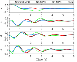
Simulation Setup. We consider a cart-pole system, where a cart of mass $m_{c}$ connects via a prismatic joint to a $1D$ track, while a pole of mass $m_{p}$ and length $2l$ is hinged to the cart. The state vector $\mathbf{x}$ includes the horizontal position of the cart $x$, the velocity of the cart $\dot{x}$, the angle of the pole with respect to vertical $\theta$, and the angular velocity of the pole $\dot{\theta}$. The control input is the force $F$ applied to the center of mass of the cart. The goal of the cart-pole is to stabilize at $(x,\dot{x},\theta,\dot{\theta})=(0,0,0,0)$. The dynamics of the cart-pole are [66]:

$$\ddot{x} =\frac{m_{p}l\left(\dot{\theta}^{2}\sin\theta-\ddot{\theta}\cos\theta\right)+F}{m_{c}+m_{p}},$$ (17)

$$\ddot{\theta} =\frac{g\sin\theta+\cos\theta\left(\frac{-m_{p}l\dot{\theta}^{2}\sin\theta-F}{m_{c}+m_{p}}\right)}{l\left(\frac{4}{3}-\frac{m_{p}\cos^{2}\theta}{m_{c}+m_{p}}\right)},$$

where $g$ is the acceleration of gravity.

To control the system, we will employ MPC at $15Hz$ with a look-ahead horizon $N=20$. We use quadratic cost functions with $Q=\mathrm{diag}\left([5.0,\;0.1,\;5.0,\;0.1]\right)$ and $R=0.1$. We use the fourth-order Runge-Kutta (RK4) method [67] for discretizing the above continuous-time dynamics. The true system parameters are $m_{c}=1.0$, $m_{p}=0.1$, and $l=0.5$ but the parameters for the nominal system dynamics are scaled to $75\%$ of the said true values. We use $M=75$ random Fourier features and $\eta=0.25$, and initialize $\hat{\alpha}$ as a zero vector —an ablation study follows in the next section. We simulate the setting for $6s$ and perform the simulation $10$ times with random initialization sampled uniformly from $x\in[-1,\;1]$, $\dot{x}\in[-0.1,\;0.1]$, $\theta\in[-0.2,\;0.2]$, $\dot{\theta}\in[-0.1,\;0.1]$. The simulation environment is based on [68] in Pybullet [69]. We use CasADi [70] to solve eq. 5.

TABLE I: Computational Performance across Different Methods for the Cart-Pole System in Section V-B. The table reports the average value and standard deviation of computational time in millisecond. The red numbers correspond to the worse performance.

	MPC	NS-MPC	GP-MPC	Ours
Time ($ms$)	$9.63\pm 3.34$	$9.94\pm 3.39$	$160.01\pm 26.96$	$16.28\pm 21.77$

TABLE II: Computational Performance across Different $M$ for our Method over the Cart-Pole System using $\eta=0.4$ in Section V-C. The table reports the average value and standard deviation of computational time in milliseconds.

$M$	$50$	$125$	$250$	$500$	$1000$
Time ($ms$)	$14.32\pm 18.80$	$23.84\pm 40.36$	$31.32\pm 71.47$	$53.16\pm 148.94$	$96.39\pm 299.99$

Compared Algorithms. We compare Algorithm 1 with an MPC that uses the (wrong) nominal system parameters (Nominal MPC), the non-stochastic MPC (NS-MPC) [41], and the Gaussian process MPC (GP-MPC) [24]. In more detail, the Nominal MPC uses the nominal dynamics to select control input by solving eq. 4. The NS-MPC augments the Nominal MPC with an additional control $v_{t}$ input that is updated by running the online gradient descent algorithm to minimize the state cost $\mathbf{x}_{t+1}Q\mathbf{x}_{t+1}^{\top}$. The GP-MPC learns $\hat{h}\left(\cdot\right)$ with a sparse Gaussian process (GP) [71, 72] whose data points are collected online, i.e., GP fixes its hyperparameters and collects data points $\left(z_{t},h\left(z_{t}\right)\right)$ online.

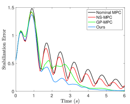
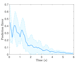
Performance Metric. We evaluate the performance of Nominal MPC, NS-MPC, GP-MPC, and Algorithm 1 in terms of their stabilization error $\|\mathbf{x}_{t}\|^{2}$ and computational time. Also, we evaluate the prediction accuracy of Algorithm 1 as we collect more data online via estimation error $e_{t}$.

Results. The results are given in Figure 2 and Table I. Figure 2(a) and Figure 2(b) demonstrate that Algorithm 1 achieves stabilization the fastest. GP-MPC comes second but it incurs a larger deviation from the stabilization goal $(0,0,0,0)$ than Algorithm 1. NS-MPC and Nominal MPC have similar performance, showing that the state-of-the-art non-stochastic control methods are insufficient when the unknown disturbance is adaptive. Figure 2(c) shows a fast convergence of the estimation error: the error decreases to around $0.1$ within $2s$ (i.e., less than $30$ iterations), which benefits our stabilization goal as shown in Figure 2(b). In Table I, Nominal MPC is the most computationally efficient, followed by NS-MPC since the online gradient descent update of $v_{t}$ only needs one projection step. GP-MPC is 16 times slower than Nominal MPC, as using GP for prediction is computationally demanding [24]. Our method maintains the expressiveness of random Fourier features such that it learns the unknown dynamics due to incorrect model parameters and is computationally efficient. For example, it is 10 times faster than GP-MPC.

(a) Circle trajectory.

(b) Wrapped Circle trajectory.

(c) Lemniscate trajectory.

(d) Wrapped Lemniscate trajectory.

Figure 4: Reference Trajectory for the Quadrotor Experiments in Section V-D. The blue lines represent the reference trajectories in $3D$. The gray lines are the projection of reference trajectories onto the ground.

(a) Circle trajectory.

(b) Wrapped Circle trajectory.

(c) Lemniscate trajectory.

(d) Wrapped Lemniscate trajectory.

Figure 5: Tracking Performance Comparison for the Quadrotor Experiments in Section V-D. Algorithm 1 demonstrates improved performance compared to Nominal MPC and GP-MPC in terms of tracking error over all tested reference trajectories and maximal speeds. Algorithm 1 with INDI achieves the best performance as INDI provides better tracking in attitude dynamics.

(a) Sample trajectories in tracking a Circle trajectory with $v_{m}=10.07\ m/s$.

(b) Sample trajectories in tracking a Lemniscate trajectory with $v_{m}=14.11\ m/s$.

Figure 6: Tracking Performance Comparison for the Quadrotor Experiments of Circle and Lemniscate Trajectories in Section V-D. The plots present the trajectories of Nominal MPC, GP-MPC, and Algorithm 1 tracking a Circle trajectory with $v_{m}=10.07\ m/s$, and a Lemniscate trajectory with $v_{m}=14.11\ m/s$, from $t=40s$ to $t=50s$ when the quadrotor reaches the maximal speeds. The trajectory of Algorithm 1 with INDI is omitted as it overlaps with Algorithm 1 w/o INDI.

V-C Sensitivity Analysis over Cart-Pole Scenario

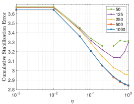
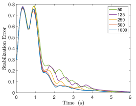
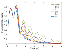
Simulation Setup. We consider the same simulation setup as in section V-B. In addition, we run the simulation with various number of random Fourier features and learning rate: we use $M\in\{50,\;125,\;250,\;500,\;1000\}$, and $\eta\in\{0.001,\;0.01,\;0.05,\;0.1,\;0.2,\;0.4,\;0.6,\;0.8,\;1\}$.

Performance Metric. We evaluate the performance of Algorithm 1 in terms of the stabilization error $\|\mathbf{x}_{t}\|^{2}$ and cumulative stabilization error $\sum_{t=1}^{T}\|\mathbf{x}_{t}\|^{2}$. Also, we consider the computational time for calculating control inputs with different $M$ while fixing $\eta$.

Results. The results are given in Figure 3 and Table II. First, we notice that Algorithm 1 has similar performance as Nominal MPC for small $\eta$, i.e., $\eta\leq 0.01$, regardless of $M$. The reason is that very small $\eta$ will keep $\hat{\alpha}$ to stay around zero. Figure 3 suggests that large $M$ and $\eta$ achieve better performance. For $M=50$ and $M=125$, increasing $\eta$ to $1$ causes worse performance, due to overshoot behaviors in estimating $\hat{\alpha}$ and, therefore, steady-state error. This can be avoided by increasing $M$. Figure 3(a) shows that the cumulative stabilization error cannot be improved after $M\geq 500$. Further, Table II shows that increasing $M$ makes the optimization problem in eq. 5 computationally expensive and prevents the method from real-time implementations, as the frequency of MPC is less than $3~{}Hz$ with $M\geq 250$ in Python.

Another tuning parameter is the standard deviation of the Gaussian distribution from which $w_{i}$ are sampled. This depends on the magnitude of feature vector $z_{t}$, since they multiply together per the definition of feature map $\Phi\left(z,\theta\right)=\phi\left(w^{\top}z+b\right)$. Hence, if $z_{t}$ has a large magnitude, the standard deviation might need to be small. Alternatively, we can normalize $z_{t}$ based on its magnitude and start tuning with a Gaussian distribution.

V-D Quadrotor Scenario

Simulation Setup. The quadrotor dynamics, the simulation environment, and the controller setup are as follows:

V-D1 Quadrotor Dynamics

$$\dot{\bm{p}} =\bm{v},\quad m\dot{\bm{v}} =m\bm{g}+\bm{f}+\bm{f}_{a},$$ (18)

$$\dot{\bm{q}} =\frac{1}{2}\bm{q}\otimes\left[\begin{array}[]{c}0\\ \bm{\omega}\end{array}\right],\quad \mathcal{J}\dot{\bm{\omega}} =-\bm{\omega}\times\mathcal{J}\bm{\omega}+\bm{\tau},$$ (21)

where $\bm{p}\in\mathbb{R}^{3}$ and $\bm{v}\in\mathbb{R}^{3}$ are position and velocity in the iniertial frame, $\bm{q}$ is the quaternion, $\otimes$ is the quaternion multiplication operator, $\bm{\omega}\in\mathbb{R}^{3}$ is the body angular velocity, $m$ is the quadrotor mass, $\mathcal{J}$ is the inertia matrix of the quadrotor, $\mathbf{g}$ is the gravity vector, $\bm{f}=\bm{R}\left[0\ 0\ T\right]^{\top}\in\mathbb{R}^{3}$ and $\bm{\tau}\in\mathbb{R}^{3}$ are the total thrust and body torques from the four rotors, $T$ is the thrust from the four rotors along the $z-$axis of the body frame, and $\bm{f}_{a}\in\mathbb{R}^{3}$ is the aerodynamic force.

V-D2 Gazebo Environment and Control Architecture

We employ the AscTec Hummingbird quadrotor model using the RotorS simulator in Gazebo [73]. The RotorS simulator implements the rotor drag as aerodynamic effects, which is a linear mapping with respect to the body frame velocity [74]. We use the following control architecture: the MPC is running at $50Hz$, takes as input the reference trajectory, and outputs the desired total thrust and desired body angular velocity to the low-level body rate controller [75, 76]; the body rate controller is running at $200Hz$, then converts them into motor speed commands to control the quadrotor in the simulator; the state of the quadrotor is available at $100Hz$.

V-D3 Control Design

The MPC uses a look-ahead horizon $N=10$ simulating the quadrotor dynamics for $1s$. We use quadratic cost functions with $Q=\mathrm{diag}\left([0.5\textbf{I}_{3},\;0.1\textbf{I}_{4},0.05\textbf{I}_{3},\;0.01\textbf{I}_{3}]\right)$ and $R=\textbf{I}_{4}$. We use the RK4 method [67] for discretization. We sample $w_{i}$ from a Gaussian distribution with standard deviation $0.01$. We use $M=50$ random Fourier features and $\eta=0.25$, and initialize $\hat{\alpha}$ as a zero vector. We use CasADi [70] and acados [77] to solve eq. 5.

V-D4 Benchmark Experiment Setup

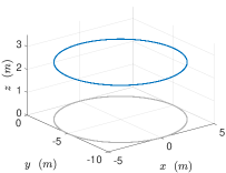
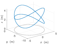
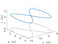
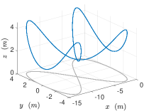
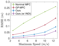
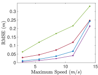
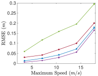
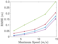
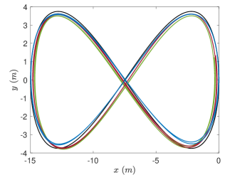
We consider that the quadrotor is tasked to track a prescribed trajectory at different maximal speeds $v_{m}$, affecting the aerodynamic forces; we consider four types of reference trajectories: Circle, Wrapped Circle, Lemniscate, and Wrapped Lemniscate, showed in Figure 4. We simulate each reference trajectory and each maximal speed 5 times. We use as the performance metric the root mean squared error (RMSE) in position.

Compared Algorithms. We compare Algorithm 1 with: a nominal MPC that assumes no aerodynamic forces (Nominal MPC), and the Gaussian process MPC (GP-MPC) [23]. The GP model in [23] is pre-trained. We adopt the default training procedure per [23]’s open-sourced code: a Nominal MPC is given $10$ random trajectories with maximal speeds $v_{m}\in[6.95,\;15.62]$; then the Nominal MPC commands the quadrotor to track these trajectories and collects the training dataset with $3556$ data points; finally, the GP model is trained such that $\bm{f}_{a}$ is predicted based on body velocities. The prediction of the GP model is used only for the first step over the look-ahead horizon. We also combine Algorithm 1 with incremental nonlinear dynamic inversion (INDI) [16] to account for unknown disturbance in the attitude dynamics in eq. 21.

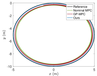
Results. The results are given in Figure 5 and Figure 6. In Figure 5, Algorithm 1 demonstrates improved performance over Nominal MPC and GP-MPC in terms of the tracking error over all tested reference trajectories and maximal speeds. The limitation of GP-MPC appears to be: (i) due to computational complexity, the prediction of GP is only used for one step in MPC; by contrast, Algorithm 1 incorporates $\hat{h}\left(\cdot\right)$ over the entire look-ahead horizon $N$; (ii) GP-MPC may not perform well if the trajectories in the training dataset are different from the executed ones; in contrast, Algorithm 1 aims to collect data and learn $\hat{h}\left(\cdot\right)$ online, thus alleviates such generalization errors. Additionally, the performance of Algorithm 1 is further improved with INDI. However, due to the low frequency in INDI control loop ($200Hz$) and state estimate ($100Hz$), the improvement is marginal especially in high-speed scenarios. Figure 6 presents the trajectories of Nominal MPC, GP-MPC, and Algorithm 1 tracking a Circle trajectory with $v_{m}=10.07\ m/s$, and a Lemniscate trajectory with $v_{m}=14.11\ m/s$, from $t=40s$ to $t=50s$ when the quadrotor reaches the maximal speeds. In Circle trajectory, Algorithm 1 clearly achieves the best tracking performance. In Lemniscate trajectory, Algorithm 1 has good tracking performance except in the corners where the quadrotor needs to turn; while Nominal MPC and GP-MPC have tracking errors along the whole trajectory.

VI Hardware Experiments

We evaluate Algorithm 1 in extensive real-world scenarios of control under uncertainty. For the experiments, we use a quadrotor as shown in Figure 7 to track a circular trajectory despite ground effects and wind disturbances (LABEL:fig_hardware). Additional results under aerodynamic drag effects and turbulent effects are given in Section -F.

Figure 7: The quadrotor for the hardware experiments.

(a) Average RMSE under Ground Effects.

(b) Average RMSE under Wind Disturbances.

(c) Average RMSE under Ground Effects & Wind Disturbances. Nominal MPC is not presented due to crash.

Figure 8: Tracking Performance Comparison for the Hardware Quadrotor Experiments in Section VI. The error bar represents the minimum and maximum RMSE. Algorithm 1 (ours) demonstrates improved performance compared to Nominal MPC and L1-MPC in terms of tracking error over all tested scenarios.

Figure 9: Tracking Performance Comparison for the Hardware Quadrotor Experiments Under Ground Effects in Section VI. The plots present sample trajectories of Nominal MPC, L1-MPC, and Algorithm 1 in $x$-, $y$-, and $z$- position (top) and the corresponding the cumulative RMSE (CRMSE) (bottom). The inserted plots present the average RMSE ($m$).

Figure 10: Tracking Performance Comparison for the Hardware Quadrotor Experiments Under Wind Disturbances in Section VI. The plots present the sample trajectories of Nominal MPC, L1-MPC, and Algorithm 1 in $x$-, $y$-, and $z$- position (top) and the corresponding CRMSE (bottom). The inserted plots present the average RMSE ($m$).

Figure 11: Tracking Performance Comparison for the Hardware Quadrotor Experiments under both Ground Effects and Wind Disturbances in Section VI. The plots present sample trajectories of L1-MPC and Algorithm 1 in $x$-, $y$-, and $z$- position (top) and the corresponding CRMSE (bottom). The inserted plots present the average RMSE ($m$). Nominal MPC is not presented since it causes crashes under both ground effects and wind disturbances.

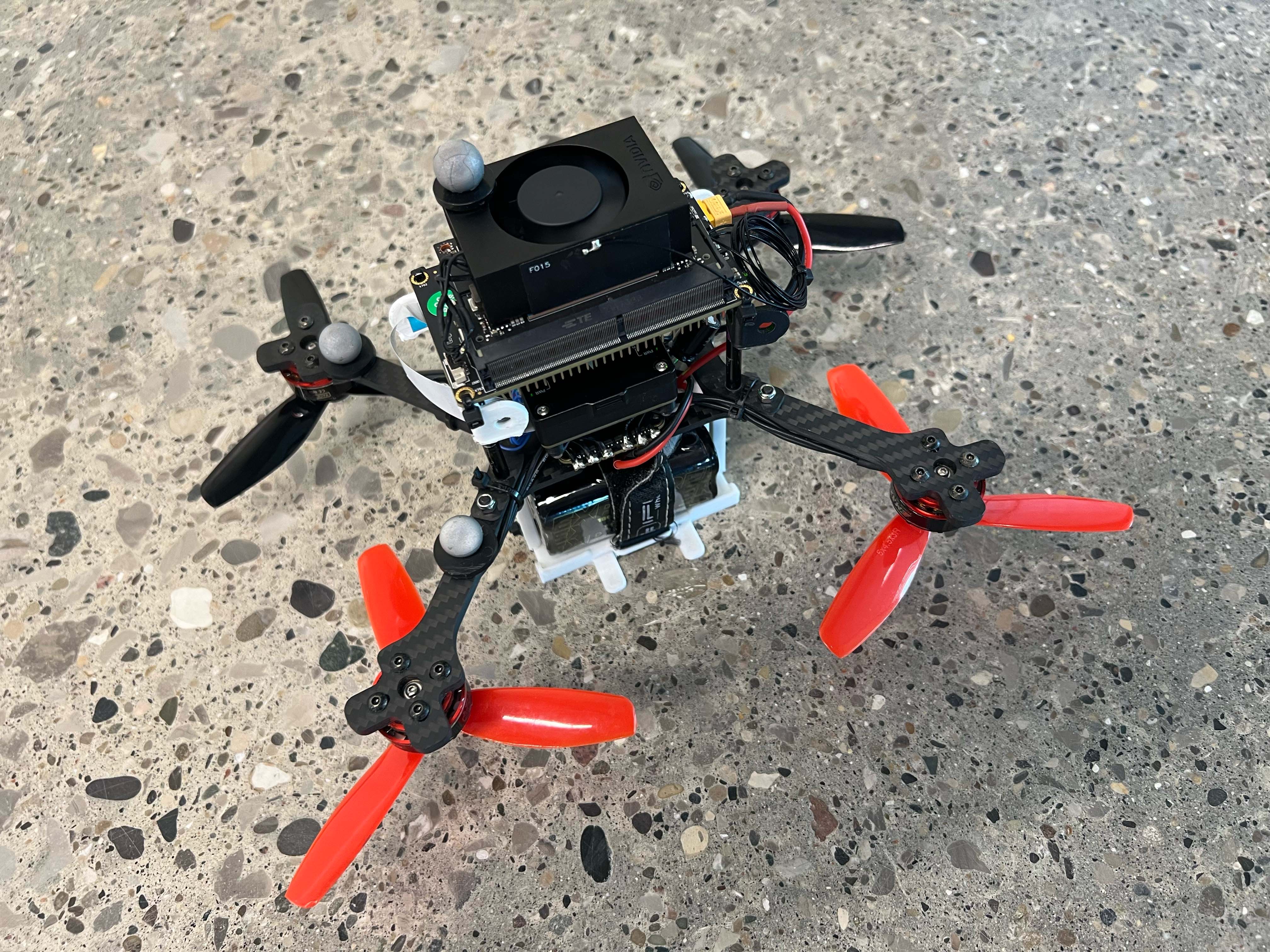
Quadrotor. The quadrotor dynamics are modeled as in eqs. 18 and 21 with weight $0.68kg$ and $0.22m$ diagonal motor-to-motor distance. The quadrotor is equipped with an Nvidia Jetson Orin NX 16GB [78] to handle on-board computation. We use the low-level controller in Holybro Pix32 v6 running PX4-Autopilot firmware [79]. The communication between Jetson Orin NX and PX4 is through MAVROS [80]. A Vicon motion capture system provides the pose of the quadrotor at $30Hz$, and we use PX4’s Extended Kalman filter to fuse the Vicon measurements with IMU readings onboard to estimate the odometry of the quadrotor. The odometry is sent to the controller at $100Hz$ and MPC runs at $50Hz$.

Control Design. We use the same MPC parameters as in Section V-D. We use $M=25$ random Fourier features and $\eta=0.05$, and initialize $\hat{\alpha}$ as a zero vector. Those parameters are fixed for all hardware experiments. We use CasADi [70] and acados [77] to solve eq. 5.

Compared Algorithms. We compare Algorithm 1 with a nominal MPC that assumes no aerodynamic forces (Nominal MPC), and the L1-adaptive MPC (L1-MPC) [17]. The L1-MPC uses the L1 adaptive control to estimate the aerodynamic force and moment in eqs. 18 and 21. Then, the MPC calculates the control input based on the estimated aerodynamic force and moment. We adopt the default parameters of estimation using L1 adaptive control per [17]’s open-sourced code.

Benchmark Experiment Setup. We consider that the quadrotor is tasked to track a circular trajectory with diameter $1m$ at maximal speed $v_{m}=0.8~{}m/s$. We consider the following disturbance scenarios:

• Ground Effects: We use an elevated foam mat to create the ground effects to the quadrotor (LABEL:fig_hardware, left). The surface of the foam mat is $0.78m$ high and the circular trajectory is set to be $0.85m$ in height. Half of the circular trajectory is above the foam mat and the other half is outside. This setting creates significant ground effects when the quadrotor is above the foam mat and a sharp transition between w/ and w/o the ground effects.

• Wind Disturbances: We use a fan to create wind disturbaces (LABEL:fig_hardware, center). The circular trajectory is at $1m$ height and its center is $3m$ away from the fan. The quadrotor experiences wind speed from $2.0~{}m/s$ to $5.4~{}m/s$ along the circular trajectory, depending on its distance to the fan. The trajectory ends at a position with wind speed from $3.5~{}m/s$ to $5.0~{}m/s$.

• Ground Effects + Wind Disturbances: We combine the previous two scenarios and now the quadrotor suffers from both ground effects and wind disturbances (LABEL:fig_hardware, right). The circular trajectory is at $0.85m$ and the wind speed varies from $1.5~{}m/s$ to $5.0~{}m/s$ along the circular trajectory. The trajectory ends at a position with wind speed from $3.3~{}m/s$ to $4.7~{}m/s$.

Additional unknown disturbances come from the battery’s voltage drop during the flight, which causes a decrease in motors’ thrust. We conduct each scenario 5 times. We use as the performance metric the RMSE in position.

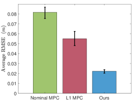
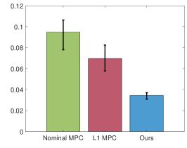
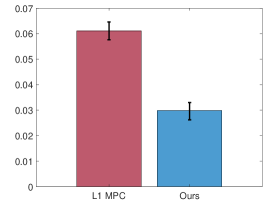
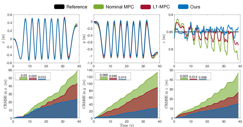
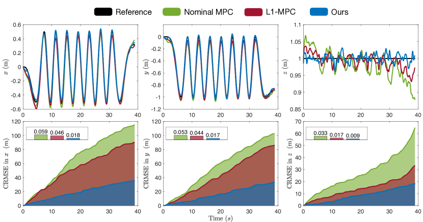
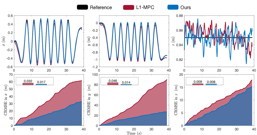
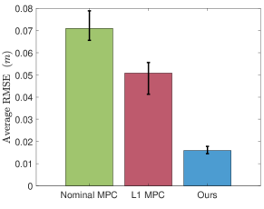
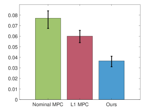
Results. The results are given in Figure 8, Figure 9, Figure 10, and Figure 11. Figure 8 shows that our algorithm achieves the best performance in average RMSE over all tested scenarios. Nominal MPC is the worst as it does not account for unknown disturbances, and it has increased $z$-direction tracking error during the flight due to insufficient thrust caused by voltage drop (Figure 9 and Figure 10, top right). Nominal MPC fails under both ground effects and wind disturbances (Figure 11) due to strong wind and voltage drop. L1-MPC has improved performance over Nominal MPC by compensating for the estimated disturbances. However, it does not account for the future evolution of the unknown disturbances and has large tracking error when the unknown disturbances change abruptly, e.g., a sharp transition between the ground and free space (Figure 9, top right). In contrast, Algorithm 1 learns the model of unknown disturbances for predictive control, and therefore, achieves the best tracking performance even when the unknown disturbances change abruptly. Algorithm 1 achieves up to $75\%$ and $60\%$ improvement in average RMSE over Nominal MPC and L1-MPC, respectively. In addition, Algorithm 1 using the same set of parameters can learn different unknown disturbances, i.e., ground effects (Figure 9), wind disturbances (Figure 10), a combination of ground effects and wind disturbances (Figure 11), and voltage drop. This is enabled by the self-supervised learning framework using the data collected online.

VII Related Work

We discuss work on system identification and control across the research topics of adaptive control; robust control; control based on offline learning; control based on offline learning combined with online adaptation; and non-stochastic control.

Adaptive control

Adaptive control methods often assume parametric uncertainty additive to the known system dynamics, e.g., parametric uncertainty in the form of unknown coefficients multiplying known basis functions [11, 12, 13]. These coefficients are updated online and generate an adaptive control input to compensate for the estimated disturbances. These methods often require persistent excitation to guarantee the exponential stability of the closed-loop system [11, 12, 13]. In contrast, inspired by [15], our method handles unknown dynamics and disturbances that can be expressed in reproductive kernel Hilbert space (RKHS), and does not require persistent excitation to enjoy near-optimality guarantees. [16, 17, 18] bypass the assumption of parametric uncertainty and persistent excitation, and directly estimate the value of unknown disturbances. However, the methods therein, as well as, the relevant method in [14, 15, 19], focus on adaptive control to compensate for the estimated disturbances, instead of learning a model of the disturbances to enable model predictive control.

Robust control

Robust control algorithms select control inputs upon simulating the future system dynamics across a lookahead horizon [5, 6, 7, 8, 9, 10]. To this end, they assume a worst-case realization of disturbances, given an upper bound to the magnitude of the disturbances [5, 6, 7, 8, 9, 10]. However, assuming the worst-case disturbances can be conservative. In addition, [6, 7, 8, 9, 10] focus on linear dynamical systems, and [8, 9, 10] may be computationally expensive. Hence, the application of these approaches is often limited to low-dimensional linear systems.

Offline learning for control

This line of work trains neural-network or Gaussian-process models using training data collected offline [21, 22, 23, 24, 25, 26, 27]. [25, 26, 27] train the models with data collected from random environments such that the controller can exhibit robustness to unseen environments [43, 44], In this paper, instead, we require no offline data collection and training, employ one-shot online learning in a self-supervised manner based on data collected online.

Offline learning and online adaption for control

Such control methods have two components: offline learning and online adaptation [28, 29, 30, 31, 32, 33, 34]. The offline learning aims to train a neural network model using data collected from different environments, e.g., the disturbances of a quadrotor under different wind speeds, so that the learned neural network model captures the underlying features across different environments. The online adaptation aims to update online either all the parameters of the neural network or only the parameters of the last layer to better predict unknown disturbances when encountering new environments. Similar to data-driven control with only offline learning, the methods need big data for effective training. Also, updating all parameters online can be computationally heavy for real-time control [28, 29, 30, 31]. [32, 33, 34] only update the last layer parameters, but either directly compensate the estimated disturbances without predicting their future evolution to optimize the controller [32, 33] or it is computationally expensive to use a neural network in on-board model predictive control [34]. In contrast, we propose to use random Fourier features to approximate online a model the unknown dynamics and disturbances. Our approach allows us to maintain the computational efficiency of classical finite-dimensional parametric approximations that can be used in model predictive control while retaining the expressiveness of the RKHS with high probability.

Non-stochastic control

Online learning algorithms, also known as non-stochastic control algorithms, select control inputs based on past information only since they assume no model that can be used to simulate the future evolution of the disturbances [35, 36, 37, 38, 39, 40, 41]. Instead, they provide controllers with bounded regret guarantees, upon employing the OCO framework to capture the non-stochastic control problem as a sequential game between a controller and an adversary [48]. They rely on the knowledge of a known upper bound to the magnitude of the disturbances, and a pre-stabilizing controller. The proposed approaches have been observed to be sensitive to the choice of the pre-stabilizing controller and the tuning parameters of OGD, e.g., in [36, 38, 40]. In contrast, our method uses OGD to learn the model of the disturbances instead of optimizing the online controller, and uses model predictive control to optimize online the control input based on the learned online disturbance model.

VIII Conclusion

We provided Algorithm 1 for the problem of Simultaneous System Identification and Model Predictive Control (1). Algorithm 1 guarantees no dynamic regret against an optimal clairvoyant (non-causal) policy that knows the disturbance function $h$ a priori. (Theorem 1). The algorithm uses random Fourier features to approximate the unknown dynamics or disturbances in reproducing kernel Hilbert spaces. Then, it employs model predictive control based on the current learned model of the unknown dynamics (or disturbances). The model of the unknown dynamics is updated online in a self-supervised manner using least squares based on the data collected while controlling the system.

We validate Algorithm 1 in simulated and hardware experiments. Our physics-based simulations include (i) a cart-pole aiming to maintain the pole upright despite inaccurate model parameters (Sections V-B and V-C), and (ii) a quadrotor aiming to track reference trajectories despite unmodeled aerodynamic drag effects (Section V-D). Our hardware experiments involve a quadrotor aiming to track a circular trajectory despite unmodeled aerodynamic drag effects, ground effects, and wind disturbances (Section VI and Section -F). We observed that our method demonstrated better tracking performance and computational efficiency than the state-of-the-art methods GP-MPC [24, 23], NS-MPC [41], and L1-MPC [17].

References

- [1] F. Cucker and S. Smale, “On the mathematical foundations of learning,” Bulletin of the American mathematical society, vol. 39, no. 1, pp. 1–49, 2002.
- [2] E. Ackerman, “Amazon promises package delivery by drone: Is it for real?” IEEE Spectrum, Web, 2013.
- [3] J. Chen, T. Liu, and S. Shen, “Tracking a moving target in cluttered environments using a quadrotor,” in 2016 IEEE/RSJ International Conference on Intelligent Robots and Systems (IROS). IEEE, 2016, pp. 446–453.
- [4] D. Seneviratne, L. Ciani, M. Catelani, D. Galar et al., “Smart maintenance and inspection of linear assets: An industry 4.0 approach,” Acta Imeko, vol. 7, pp. 50–56, 2018.
- [5] D. Q. Mayne, M. M. Seron, and S. Raković, “Robust model predictive control of constrained linear systems with bounded disturbances,” Automatica, vol. 41, no. 2, pp. 219–224, 2005.
- [6] G. Goel and B. Hassibi, “Regret-optimal control in dynamic environments,” arXiv preprint:2010.10473, 2020.
- [7] O. Sabag, G. Goel, S. Lale, and B. Hassibi, “Regret-optimal full-information control,” arXiv preprint:2105.01244, 2021.
- [8] A. Martin, L. Furieri, F. Dörfler, J. Lygeros, and G. Ferrari-Trecate, “Safe control with minimal regret,” in Learning for Dynamics and Control Conference (L4DC), 2022, pp. 726–738.
- [9] A. Didier, J. Sieber, and M. N. Zeilinger, “A system level approach to regret optimal control,” IEEE Control Systems Letters (L-CSS), 2022.
- [10] H. Zhou and V. Tzoumas, “Safe control of partially-observed linear time-varying systems with minimal worst-case dynamic regret,” in 2023 62nd IEEE Conference on Decision and Control (CDC). IEEE, 2023, pp. 8781–8787.
- [11] J.-J. E. Slotine, “Applied nonlinear control,” PRENTICE-HALL google schola, vol. 2, pp. 1123–1131, 1991.
- [12] M. Krstic, P. V. Kokotovic, and I. Kanellakopoulos, Nonlinear and adaptive control design. John Wiley & Sons, Inc., 1995.
- [13] P. A. Ioannou and J. Sun, Robust adaptive control. PTR Prentice-Hall Upper Saddle River, NJ, 1996, vol. 1.
- [14] N. M. Boffi, S. Tu, and J.-J. E. Slotine, “Regret bounds for adaptive nonlinear control,” in Learning for Dynamics and Control. PMLR, 2021, pp. 471–483.
- [15] ——, “Nonparametric adaptive control and prediction: Theory and randomized algorithms,” Journal of Machine Learning Research, vol. 23, no. 281, pp. 1–46, 2022.
- [16] E. Tal and S. Karaman, “Accurate tracking of aggressive quadrotor trajectories using incremental nonlinear dynamic inversion and differential flatness,” IEEE Transactions on Control Systems Technology, vol. 29, no. 3, pp. 1203–1218, 2020.
- [17] Z. Wu, S. Cheng, P. Zhao, A. Gahlawat, K. A. Ackerman, A. Lakshmanan, C. Yang, J. Yu, and N. Hovakimyan, “L1 quad: L1 adaptive augmentation of geometric control for agile quadrotors with performance guarantees,” arXiv preprint arXiv:2302.07208, 2023.
- [18] E. Das and J. W. Burdick, “Robust control barrier functions using uncertainty estimation with application to mobile robots,” arXiv preprint arXiv:2401.01881, 2024.
- [19] J. Jia, W. Zhang, K. Guo, J. Wang, X. Yu, Y. Shi, and L. Guo, “Evolver: Online learning and prediction of disturbances for robot control,” IEEE Transactions on Robotics, 2023.
- [20] Y. Rahman, A. Xie, J. B. Hoagg, and D. S. Bernstein, “A tutorial and overview of retrospective cost adaptive control,” in 2016 American Control Conference (ACC). IEEE, 2016, pp. 3386–3409.
- [21] C. Sánchez-Sánchez and D. Izzo, “Real-time optimal control via deep neural networks: study on landing problems,” Journal of Guidance, Control, and Dynamics, vol. 41, no. 5, pp. 1122–1135, 2018.
- [22] A. Carron, E. Arcari, M. Wermelinger, L. Hewing, M. Hutter, and M. N. Zeilinger, “Data-driven model predictive control for trajectory tracking with a robotic arm,” IEEE Robotics and Automation Letters, vol. 4, no. 4, pp. 3758–3765, 2019.
- [23] G. Torrente, E. Kaufmann, P. Föhn, and D. Scaramuzza, “Data-driven mpc for quadrotors,” IEEE Robotics and Automation Letters, vol. 6, no. 2, pp. 3769–3776, 2021.
- [24] L. Hewing, J. Kabzan, and M. N. Zeilinger, “Cautious model predictive control using gaussian process regression,” IEEE Transactions on Control Systems Technology, vol. 28, no. 6, pp. 2736–2743, 2019.
- [25] J. Tobin, R. Fong, A. Ray, J. Schneider, W. Zaremba, and P. Abbeel, “Domain randomization for transferring deep neural networks from simulation to the real world,” in 2017 IEEE/RSJ international conference on intelligent robots and systems (IROS). IEEE, 2017, pp. 23–30.
- [26] F. Ramos, R. C. Possas, and D. Fox, “Bayessim: adaptive domain randomization via probabilistic inference for robotics simulators,” arXiv preprint arXiv:1906.01728, 2019.
- [27] J. Lee, J. Hwangbo, L. Wellhausen, V. Koltun, and M. Hutter, “Learning quadrupedal locomotion over challenging terrain,” Science robotics, vol. 5, no. 47, p. eabc5986, 2020.
- [28] C. Finn, P. Abbeel, and S. Levine, “Model-agnostic meta-learning for fast adaptation of deep networks,” in International conference on machine learning. PMLR, 2017, pp. 1126–1135.
- [29] G. Williams, N. Wagener, B. Goldfain, P. Drews, J. M. Rehg, B. Boots, and E. A. Theodorou, “Information theoretic mpc for model-based reinforcement learning,” in 2017 IEEE international conference on robotics and automation (ICRA). IEEE, 2017, pp. 1714–1721.
- [30] A. Nagabandi, I. Clavera, S. Liu, R. S. Fearing, P. Abbeel, S. Levine, and C. Finn, “Learning to adapt in dynamic, real-world environments through meta-reinforcement learning,” arXiv preprint arXiv:1803.11347, 2018.
- [31] S. Belkhale, R. Li, G. Kahn, R. McAllister, R. Calandra, and S. Levine, “Model-based meta-reinforcement learning for flight with suspended payloads,” IEEE Robotics and Automation Letters, vol. 6, no. 2, pp. 1471–1478, 2021.
- [32] G. Shi, X. Shi, M. O’Connell, R. Yu, K. Azizzadenesheli, A. Anandkumar, Y. Yue, and S.-J. Chung, “Neural lander: Stable drone landing control using learned dynamics,” in 2019 International Conference on Robotics and Automation (ICRA). IEEE, 2019, pp. 9784–9790.
- [33] M. O’Connell, G. Shi, X. Shi, K. Azizzadenesheli, A. Anandkumar, Y. Yue, and S.-J. Chung, “Neural-fly enables rapid learning for agile flight in strong winds,” Science Robotics, vol. 7, no. 66, p. eabm6597, 2022.
- [34] A. Saviolo, J. Frey, A. Rathod, M. Diehl, and G. Loianno, “Active learning of discrete-time dynamics for uncertainty-aware model predictive control,” IEEE Transactions on Robotics, 2023.
- [35] E. Hazan and K. Singh, “Introduction to online nonstochastic control,” arXiv preprint arXiv:2211.09619, 2022.
- [36] N. Agarwal, B. Bullins, E. Hazan, S. Kakade, and K. Singh, “Online control with adversarial disturbances,” in International Conference on Machine Learning (ICML), 2019, pp. 111–119.
- [37] P. Zhao, Y.-X. Wang, and Z.-H. Zhou, “Non-stationary online learning with memory and non-stochastic control,” in International Conference on Artificial Intelligence and Statistics (AISTATS). PMLR, 2022, pp. 2101–2133.
- [38] P. Gradu, E. Hazan, and E. Minasyan, “Adaptive regret for control of time-varying dynamics,” arXiv preprint:2007.04393, 2020.
- [39] H. Zhou, Z. Xu, and V. Tzoumas, “Efficient online learning with memory via frank-wolfe optimization: Algorithms with bounded dynamic regret and applications to control,” in 2023 62nd IEEE Conference on Decision and Control (CDC). IEEE, 2023, pp. 8266–8273.
- [40] H. Zhou and V. Tzoumas, “Safe non-stochastic control of linear dynamical systems,” in 2023 62nd IEEE Conference on Decision and Control (CDC). IEEE, 2023, pp. 5033–5038.
- [41] H. Zhou, Y. Song, and V. Tzoumas, “Safe non-stochastic control of control-affine systems: An online convex optimization approach,” IEEE Robotics and Automation Letters, 2023.
- [42] H. A. Pierson and M. S. Gashler, “Deep learning in robotics: a review of recent research,” Advanced Robotics, vol. 31, no. 16, pp. 821–835, 2017.
- [43] M. Mohri, A. Rostamizadeh, and A. Talwalkar, Foundations of machine learning. MIT press, 2018.
- [44] Y. S. Abu-Mostafa, M. Magdon-Ismail, and H.-T. Lin, Learning from data. AMLBook New York, 2012, vol. 4.
- [45] K. Zhou and J. C. Doyle, Essentials of robust control. Prentice hall Upper Saddle River, NJ, 1998, vol. 104.
- [46] E. Lavretsky and K. A. Wise, “Robust adaptive control,” in Robust and adaptive control: With aerospace applications. Springer, 2012, pp. 317–353.
- [47] S. Sun, A. Romero, P. Foehn, E. Kaufmann, and D. Scaramuzza, “A comparative study of nonlinear mpc and differential-flatness-based control for quadrotor agile flight,” IEEE Transactions on Robotics, vol. 38, no. 6, pp. 3357–3373, 2022.
- [48] E. Hazan et al., “Introduction to online convex optimization,” Foundations and Trends in Optimization, vol. 2, no. 3-4, pp. 157–325, 2016.
- [49] A. Rahimi and B. Recht, “Random features for large-scale kernel machines,” Advances in neural information processing systems, vol. 20, 2007.
- [50] ——, “Uniform approximation of functions with random bases,” in 2008 46th annual allerton conference on communication, control, and computing. IEEE, 2008, pp. 555–561.
- [51] S. Lale, K. Azizzadenesheli, B. Hassibi, and A. Anandkumar, “Model learning predictive control in nonlinear dynamical systems,” in 2021 60th IEEE Conference on Decision and Control (CDC). IEEE, 2021, pp. 757–762.
- [52] A. Karapetyan, E. C. Balta, A. Tsiamis, A. Iannelli, and J. Lygeros, “On the regret of recursive methods for discrete-time adaptive control with matched uncertainty,” arXiv preprint arXiv:2404.02023, 2024.
- [53] D. Muthirayan, J. Yuan, D. Kalathil, and P. P. Khargonekar, “Online learning for predictive control with provable regret guarantees,” in 2022 IEEE 61st Conference on Decision and Control (CDC). IEEE, 2022, pp. 6666–6671.
- [54] F. Bach, “Breaking the curse of dimensionality with convex neural networks,” Journal of Machine Learning Research, vol. 18, no. 19, pp. 1–53, 2017.
- [55] C. Carmeli, E. De Vito, A. Toigo, and V. Umanitá, “Vector valued reproducing kernel hilbert spaces and universality,” Analysis and Applications, vol. 8, no. 01, pp. 19–61, 2010.
- [56] R. Brault, M. Heinonen, and F. Buc, “Random fourier features for operator-valued kernels,” in Asian Conference on Machine Learning. PMLR, 2016, pp. 110–125.
- [57] M. Nonhoff and M. A. Müller, “On the relation between dynamic regret and closed-loop stability,” arXiv preprint arXiv:2209.05964, 2022.
- [58] J. B. Rawlings, D. Q. Mayne, and M. Diehl, Model predictive control: Theory, computation, and design. Nob Hill Publishing, 2017, vol. 2.
- [59] F. Borrelli, A. Bemporad, and M. Morari, Predictive control for linear and hybrid systems. Cambridge University Press, 2017.
- [60] G. Grimm, M. J. Messina, S. E. Tuna, and A. R. Teel, “Model predictive control: for want of a local control lyapunov function, all is not lost,” IEEE Transactions on Automatic Control, vol. 50, no. 5, pp. 546–558, 2005.
- [61] T. Cunis, I. Kolmanovsky, and C. E. Cesnik, “Integrating nonlinear controllability into a multidisciplinary design process,” Journal of Guidance, Control, and Dynamics, vol. 46, no. 6, pp. 1026–1037, 2023.
- [62] A. A. Agrachev, A. S. Morse, E. D. Sontag, H. J. Sussmann, V. I. Utkin, and E. D. Sontag, “Input to state stability: Basic concepts and results,” Nonlinear and optimal control theory: lectures given at the CIME summer school held in Cetraro, Italy June 19–29, 2004, pp. 163–220, 2008.
- [63] H. K. Khalil, Nonlinear control. Pearson New York, 2015, vol. 406.
- [64] H. Q. Minh, “Operator-valued bochner theorem, fourier feature maps for operator-valued kernels, and vector-valued learning,” arXiv preprint arXiv:1608.05639, 2016.
- [65] Y. Bengio, N. Roux, P. Vincent, O. Delalleau, and P. Marcotte, “Convex neural networks,” Advances in neural information processing systems, vol. 18, 2005.
- [66] R. V. Florian, “Correct equations for the dynamics of the cart-pole system,” Center for Cognitive and Neural Studies (Coneural), Romania, p. 63, 2007.
- [67] P. E. Kloeden, E. Platen, P. E. Kloeden, and E. Platen, Stochastic differential equations. Springer, 1992.
- [68] Z. Yuan, A. W. Hall, S. Zhou, L. Brunke, M. Greeff, J. Panerati, and A. P. Schoellig, “Safe-control-gym: A unified benchmark suite for safe learning-based control and reinforcement learning in robotics,” IEEE Robotics and Automation Letters, vol. 7, no. 4, pp. 11 142–11 149, 2022.
- [69] E. Coumans and Y. Bai, “Pybullet, a python module for physics simulation for games, robotics and machine learning,” 2016.
- [70] J. A. Andersson, J. Gillis, G. Horn, J. B. Rawlings, and M. Diehl, “Casadi: a software framework for nonlinear optimization and optimal control,” Mathematical Programming Computation, vol. 11, pp. 1–36, 2019.
- [71] J. Quinonero-Candela and C. E. Rasmussen, “A unifying view of sparse approximate gaussian process regression,” The Journal of Machine Learning Research, vol. 6, pp. 1939–1959, 2005.
- [72] E. Snelson and Z. Ghahramani, “Sparse gaussian processes using pseudo-inputs,” Advances in neural information processing systems, vol. 18, 2005.
- [73] F. Furrer, M. Burri, M. Achtelik, and R. Siegwart, Robot Operating System (ROS): The Complete Reference (Volume 1). Cham: Springer International Publishing, 2016, ch. RotorS—A Modular Gazebo MAV Simulator Framework, pp. 595–625. [Online]. Available: http://dx.doi.org/10.1007/978-3-319-26054-9_23
- [74] P. Martin and E. Salaün, “The true role of accelerometer feedback in quadrotor control,” in 2010 IEEE international conference on robotics and automation. IEEE, 2010, pp. 1623–1629.
- [75] M. Faessler, D. Falanga, and D. Scaramuzza, “Thrust mixing, saturation, and body-rate control for accurate aggressive quadrotor flight,” IEEE Robotics and Automation Letters, vol. 2, no. 2, pp. 476–482, 2016.
- [76] M. Faessler, A. Franchi, and D. Scaramuzza, “Differential flatness of quadrotor dynamics subject to rotor drag for accurate tracking of high-speed trajectories,” IEEE Robotics and Automation Letters, vol. 3, no. 2, pp. 620–626, 2017.
- [77] R. Verschueren, G. Frison, D. Kouzoupis, J. Frey, N. v. Duijkeren, A. Zanelli, B. Novoselnik, T. Albin, R. Quirynen, and M. Diehl, “acados—a modular open-source framework for fast embedded optimal control,” Mathematical Programming Computation, vol. 14, no. 1, pp. 147–183, 2022.
- [78] D. C. Youvan, “Developing and deploying ai applications on nvidia jetson orin nx: A comprehensive guide,” 2024.
- [79] “Px4 autopilot: Open source autopilot for drones.” [Online]. Available: https://docs.px4.io/main/en/index.html
- [80] “Mavros: Communication driver for autopilots with mavlink communication protocol.” [Online]. Available: https://wiki.ros.org/mavros#Overview
- [81] A. Tsiamis, A. Karapetyan, Y. Li, E. C. Balta, and J. Lygeros, “Predictive linear online tracking for unknown targets,” arXiv preprint arXiv:2402.10036, 2024.