FIP-GNN: Graph neural networks for scalable prediction of grain-level fatigue indicator parameters

Abstract

High-cycle fatigue is a critical performance metric of structural alloys for many applications. The high cost, time, and labor involved in experimental fatigue testing call for efficient and accurate computer models of fatigue life. We present graph neural networks for polycrystals that, for the first time, can (i) predict fatigue indicator parameters – grain-level responses to cyclic loading well beyond monotonic elastic and inelastic regimes reported in literature; and (ii) generalize these predictions to large microstructure volume elements with grain populations well beyond those used in training. These advances can make significant contributions to statistically rigorous and computationally efficient modeling of high-cycle fatigue – a long-standing challenge in the field.

Understanding and predicting fatigue are crucial in the design and qualification of advanced structural alloys. Determination of the lifespan of alloys in high cycle fatigue (HCF) is especially challenging due to its high variability [1] and the need in time-consuming mechanical tests to a large number of cycles required for crack initiation. The cost, time, and labor involved in experimental HCF testing highlights the need in efficient and accurate computer models.

One of the approaches to modeling HCF aims to compute the driving force for crack initiation because it is the crack initiation, rather than growth, accounts for most of the HCF life in polycrystalline alloys [2]. The driving force is typically quantified by fatigue indicator parameter (FIP) calculated in microstructure-based full-field simulations, e.g., with the crystal plasticity finite element method (CPFE) method [3]. Calculation of FIPs most predictive of crack initiation observed in experiments has been the subject of intensive research [4], and multiple FIPs have been introduced to date [3, 5, 6, 7, 8]. The Fatemi–Socie FIP is one of the most widely used FIPs because it has relatively small mesh sensitivity [9] and does not require explicit implementation of the crack tip, allowing the FIP calculation within purely continuum CPFE simulations. Utilizing the Fatemi–Socie FIP as a metric of spatially resolved driving force for crack initiation, Przybyla et al. [10] developed a methodology of evaluating and ranking microstructures in terms of their resistance to HCF. Their approach is based on statistical analysis of FIP values in polycrystals represented by microstructure volume elements (MVEs). A challenge in the methodology is that statistical analysis of most interest for the HCF resistance focuses on the extreme value (EV) distributions that require MVEs prohibitively large for CPFE simulations. For example, for an Al 7075-T6 alloy, MVEs containing even $10^{6}$ grains were still reported insufficiently representative for FIP EV distributions, which is already impractically expensive – a CPFE simulation on a single MVE with only 1000 grains requires more than 100 CPU hours [11]. Given the high computational cost of the CPFE method and the need in large populations of grains for EV distributions, researchers adopted the concept of statistical volume elements (SVEs), where multiple MVEs are used for simulations to represent one microstructure in lieu of a single large MVE [12, 13, 14]. With this approach, EV distributions of FIPs can be obtained from a large number of grains in an SVE of a microstructure of interest, which, however, still comes at a high computational cost associated with CPFE simulations on multiple MVEs.

The high computational cost of the CPFE method for statistically rigorous modeling of HCF emphasizes the need in new efficient approaches. Machine learning is one of the routes towards reducing the computational cost of modeling microstructure–property relationships in materials. A machine learning strategy extensively explored in literature is the development of surrogate models that can reproduce the results of computationally demanding direct numerical simulations such as CPFEM at a fraction of their computational cost. Quite a few surrogate models have been reported to date [15, 16, 14, 17, 18, 19, 20, 21, 22, 23, 24, 25, 26, 27, 28, 29], and they primarily differ in their approach to quantitative description of microstructure. Reported approaches include the description by spatial correlations [15, 16, 14], latent representation by convolutional neural networks learned during training [30, 17, 18], and graphs [19, 20, 21, 22, 23, 24, 25, 26, 27, 28, 29]. Graph representation of polycrystals and the subsequent use of graph neural networks (GNNs) have been recently gaining momentum. Compared to other descriptions, graph representation does not require full 3D voxel-to-voxel data yet captures the overall grain structure and its connectivity in polycrystals. Graph representation and GNNs have been successful in modeling a range of properties of polycrystals, both mechanical [19, 20, 21, 22, 23, 24, 25, 29] and non-mechanical [26, 27, 28]. To cite a few studies relevant to micromechanics, Vlassis et al. [19] developed GNN models to predict the elastic energy functional of materials described by hyperelastic constitutive laws. Pagan et al. [20] trained GNNs to predict grain-average stress in Ni and Ti alloys using data from CPFE simulations and experiments. Sadeghpour et al. [21] modeled the offset yield strength of 316L steel, while Hestroffer et al. [22] developed GNNs for the effective yield strength and elastic modulus of $\alpha$-Ti microstructures with various crystallographic textures. Hu and Latypov [25] generalized GNNs ability to predict anisotopic effective properties to arbitrary loading directions. Hu et al. [29] proposed a temporal GNN model that integrates a GNN with recurrent neural networks to predict orientation evolution paths and stress history of each grain in a polycrystal. These studies demonstrate the potential of GNNs for modeling micromechanics of polycrystals, both in terms of their overall properties and grain-level responses. In this context, GNNs are promising for computationally efficient prediction of grain-level FIPs. At the same time, most GNN studies to date modeled micromechanical polycrystal responses in purely elastic and initial yield regimes or under monotonic loading. The predictive power of GNNs beyond of highly non-linear responses such as FIPs and under cyclic loading is currently unknown.

Figure 1: Pictorial overview of this study, including training and optimization of GNNs with small MVEs (MVE30 set), GNN architecture, and large MVEs used for testing the predictive capabilities of GNNs for modeling grain-level FIPs in large MVEs. MVE sets (MVE30, MVE45, …, MVE250) are labeled according to the number of voxels (“vox.”) along one side of the cube MVEs. Only one example MVE is visualized for each set, total number of MVEs (“samples”) and approximate number of grains, $N$, for each MVE size are also provided.

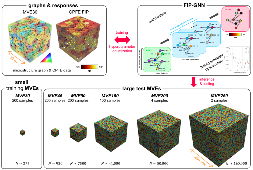
In this study, we demonstrate the ability of GNNs to model grain-level FIPs as non-linear micromechanical responses of polycrystals under cyclic loading. We demonstrate that GNNs can tackle the challenge of modeling FIPs in large MVEs with large grain populations at a modest computational cost. To this end, we trained GNNs using publicly available dataset on an Al 7075-T6 alloy [31] featuring CPFE simulation results by Stopka, Yaghoobi et al. [32, 33]. The dataset includes computer-generated MVEs of various sizes ($30^{3}$ to to $250^{3}$ voxels, see Figure 1) and grain counts ($275\text{\,}$ to $160\,000\text{\,}$) and their micromechanical responses from CPFE simulations, including spatially-resolved FIPs. For each MVE, we created a microstructure graph, wherein grains are represented by graph nodes, while grain boundaries are represented by graph edges that link nodes corresponding to adjacent grains. We incorporated different grain properties as feature sets to nodes in these graphs, including (i) Euler angles and (ii) quaternions – both representing grain orientations – as well as (iii) Schmid factors calculated for each grain respect to the loading direction. We further calculated grain-level Fatemi–Socie FIP values by averaging the maximum values from all CPFE integration points in a grain as the node response for learning and inference. We trained and optimized the GNNs with the three feature choices using a set of 200 smallest MVEs (MVE30) and then tested the capabilities of the trained models to predict grain-level FIPs in large MVEs. A sketch of the FIP-GNN is shown in Figure 1, further descriptions of the GNN model, data, training, and hyperparameter optimization are detailed in the Data and Methods section.

Figure 2: Parity plots comparing grain-level FIPs predicted by the GNN vs. those from CPFE simulations for 20 microstructures from the MVE30-VAL set. The parity plots are shown for three GNNs with optimizerd hyperparameters ($n$ and $k$) based on (a) Euler angles, (b) quaternions, (c) 12 Schmid factors as graph node features. The corresponding meanARE and $R^{2}$ as well as the number of learnable weights and number of epochs to reach a plateau in the validation loss are also shown.

Figure 3: Results of hyperparameter optimization, training, and inference for the GNN model trained with 12 Schmid factors as features: (a) mean squared error for a validation set (MVE30-VAL) obtained for different combinations of the number of nodes in the hidden layer, $n$, and the number of message passing layers, $k$; (b) grain-level FIP fields predicted by GNN and obtained in CPFE simulations.

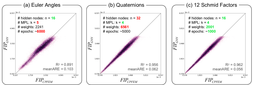
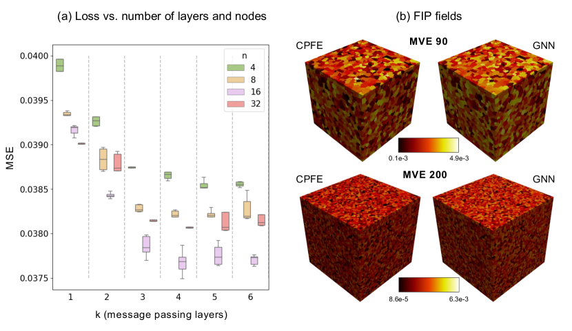
We first compare GNNs trained with different choices of the node features: Euler angles, quaternions, and Schmid factors. To this end, we split the MVE30 set to 180 training MVEs and 20 validation MVEs to optimize GNN hyperparameters and evaluate the impact of the feature choice on the GNN performance. All three GNNs capture grain-level FIPs with $R^{2}>0.89$ and with mean average relative error (meanARE) within $10\text{\,}\mathrm{\char 37\relax}$(Figure 2). Among the three models, the GNN that uses Euler angles as features shows the lowest accuracy (Figure 2a). While the GNNs trained with quaternions and Schmid factors both have superior accuracy, the GNN relying on quaternions (Figure 2b) includes more than three times more learnable weights to reach the accuracy comparable with the GNN using Schmid factors (Figure 2c). The difference in the number of weights arise because we optimized hyperparameters (primarily $n$ and $k$, see Figure 1 and Figure 3a) individually for each model and the GNN with quaternions has the highest optimal number of nodes in the hidden layer, $n=32$, among the three models (Figure 2). Further, the GNN with Schmid factors learns fastest among the three models with only $1000\text{\,}$ epochs needed to reach the plateau in the validation error, as opposed to the $5000\text{\,}$ to $6000\text{\,}$ epoch range for the GNNs based on orientations as node features. Since Schmid factors as features lead to the best combination of accuracy, size, and learning speed in GNNs, we focus on developing GNNs for FIPs using Schmid factors as the node features of choice for the remainder of the study.

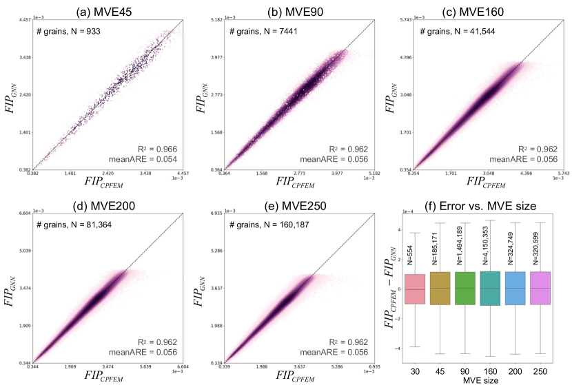
We next evaluate the capability of GNNs to generalize FIP predictions to large MVEs with grain populations well beyond those used in training. To this end, we trained the best GNN identified above (Schmid factors as features and optimized $n$ and $k$ hyperparameters) on the entire MVE30 set and then evaluated its accuracy on MVEs of progressively increasing size from $45^{3}$ to $250^{3}$ voxels. Predictions for one MVE from each of five size sets shows that the GNN can predict grain-level FIP values for large MVEs with a wide range of grain populations significantly exceeding those the GNN has “seen” during training (Figure 4). Indeed, the GNN shows a consistent overall accuracy of $R^{2}>0.96$ for five MVEs of all studied sizes and the corresponding grain populations. To support this result, we extend this analysis to all MVEs from each size set and visually summarize the results in a box plot of error distributions (Figure 4f). We find that the difference in grain-level FIPs predicted by the GNN from high-fidelity CPFE values has a mean close to zero consistently across all studied MVE sizes. The range of the error does not correlate with the MVE size, which once again attests to the GNNs ability to predict GNNs for MVEs with large grain populations with consistent accuracy. Finally, the field of FIPs predicted by GNN and mapped to a couple of example MVEs also show good visual agreement with the CPFE fields (Figure 3b).

Figure 4: Evaluation of the capability of the GNN trained on 200 microstructures of the MVE30 set to predict FIPs in larger MVEs shown as (a-e) parity plots comparing GNN FIPs with ground truth values from CPFE simulations for individual MVEs of increasing size; (f) box plot showing the distribution of the difference in predicted FIPs from ground truth values.

The presented GNN approach enables not only response predictions but also insights into micromechanics relevant to HCF reflected by FIPs. The use of 12 Schmid factors calculated for each grain as node features resulted in the most accurate GNN model (Figure 2) with a minimum number of learnable weights. Here, one may wonder if all 12 Schmid factors are necessary for an accurate prediction of grain-level FIPs. To address this question, we tested the accuracy of the GNN model using Schmid factors for only three most active slip systems for each grain. With three highest Schmid factors per grain as features, we obtain a GNN model with $R^{2}=0.956$ for the MVE30-VAL set. This accuracy is only marginally lower than the GNN trained on the full set of 12 Schmid factors and nearly identical to that of the GNN model using quaternions (Figure 2b-c). This surprisingly good accuracy of a GNN that uses only three Schmid factors suggests that the driving force for crack initiation quantified by FIPs is associated with slip activity on very few dominant systems. This is consistent with arguments in literature that few slip systems get activated in each grain during deformation of polycrystals [34]. In fact, our additional tests showed that using only one and two Schmid factors for most active systems still allows FIP predictions with $R^{2}>0.8$. In addition, the result with fewer Schmid factors indicates that the GNN with Schmid factors as features showed better accuracy than orientations (Figure 2) not simply because of greater number of node features. This clearly follows from the identical accuracy of the GNN with three Schmid factors as three features ($R^{2}=0.956$) compared to the GNN with quaternions as four features ($R^{2}=0.956$). Use of Schmid factors leading to more accurate GNNs than GNNs using orientations at the same or smaller number of features can be attributed to more direct relevance to the response of interest (FIPs) and better compatibility with convolution functions in GNNs [25]. While Schmid factors sufficed in this study of FIPs in polycrystals under uniaxial cycling loading, elements of full Schmid tensors (as in [25]) can serve as features for modeling HCF under more complex (multi-axial) loading conditions.

We can gain further insight into the role of local microstructure in FIP and crack initiation from the architecture of the GNN architecture optimized as part of this study. Our hyperparameter optimization included identification of the optimal number of message passing layers, $k$. Each message passing layer aggregates features from the nearest-neighbor nodes in the graph [35] so that stacking $k$ layers aggregates features from neighbors of the $k^{\text{th}}$ order, i.e., graph nodes $k$ edges apart. In terms of polycrystal micromechanics, $k$ signifies the order of the neighbor grains that affect the response (FIP) in any give grain. From our hyperparameter optimization, we found $k=4$ layers as optimal for predicting grain-level FIPs (see Figure 3a). It means that accounting for Schmid factors up to fourth-order nearest neighbors is needed for FIP predictions with the high accuracy reported above. This purely data-driven result is consistent with explicit studies of the impact of grain neighborhood on FIPs using physics-based CPFE simulations. Stopka et al. [32] studied the impact of altering neighboring grains on the FIPs in the same Al 7075-T6 alloy. The authors found that the FIP value in a “hot-spot” grain is sensitive to the orientations of the nearest neighbor grains of up to fourth order. Similarly, our results show that accounting for features from grains more than four edges away (using $k>4$) did not improve the accuracy of FIP predictions (Figure 3a).

In conclusion, we developed GNNs for polycrystals that, for the first time, can (i) predict FIPs – grain-level responses to cyclic loading well beyond monotonic elastic and inelastic regimes reported in literature; and (ii) generalize these predictions to MVEs with grain populations significantly larger than MVEs used in training. These advances can make significant contributions to statistically rigorous and computationally efficient modeling of HCF – a long standing challenge in the field. The computational gain with presented GNNs is two-fold: (i) GNNs can serve as orders of magnitude faster surrogates to CPFE simulations of FIPs and (ii) GNNs can obtain FIPs and their distributions from very large MVEs out of reach for direct CPFE simulations. Indeed, FIP inference with a trained GNN took no more than $200\text{\,}\mathrm{ms}$ for the largest MVEs considered in this study (MVE250) and as little as $2.5\text{\,}\mathrm{ms}$ for samples from the MVE30 set on a consumer-grade workstation. In comparison, direct CPFE simulations of the same FIPs after cyclic loading require over 100 hours for one sample of the MVE90 set on a single CPU [11]. In addition, unlike CPFE simulations [36], the proposed GNN models exhibit $O(N)$ complexity, i.e., their computational cost increases linearly with the number of grains, $N$, in an MVE. The moderate computational complexity and the generalization capability of GNNs to large grain populations demonstrated in this study opens opportunities for rapid calculation of statistically significant FIP EV distributions in microstructures for their ranking in terms of HCF resistance and design for superior HCF life. We also demonstrated that the GNN approach provides insights into the variables relevant to micromechanical response of polycrystals during HCF loading consistent with prior physics-based CPFE modeling.

Data and methods

This section provides the details on the (i) data used for training and testing; (ii) microstructure representation with graphs; (iii) GNN architecture design; (iv) GNN training, hyper-parameter tuning, and validation.

Data

For training GNNs in this study, we made use of a dataset published by Stopka and Yaghoobi [31], which contains an ensemble of polycrystalline MVEs and the micromechanical data from CPFE simulations carried out on these MVEs. The MVEs represent 3D polycrystalline aggregates of an Al 7075-T6 alloy with predominantly equiaxed microstructure and uniform texture [33]. The grain size of the MVEs follows a lognormal distribution with an average equivalent grain diameter of $14\text{\,}\mathrm{\SIUnitSymbolMicro m}$ and its standard deviation of $2\text{\,}\mathrm{\SIUnitSymbolMicro m}$. The crystallographic orientation of each grain in the dataset is described by Euler angles in the ZXZ convention. The dataset contains six subsets of MVEs differentiated by their size that cover a broad spectrum of grain populations. The subsets correspond to six MVE sizes with $30\text{\,}$, $45\text{\,}$, $90\text{\,}$, $160\text{\,}$, $200\text{\,}$, and $250\text{\,}$ voxels along each of the three principal axes. These sizes correspond to the average grain counts per MVE of about $280\text{\,}$, $930\text{\,}$, $7500\text{\,}$, $41\,000\text{\,}$, $80\,000\text{\,}$, and $160\,000\text{\,}$ grains, respectively. We refer to these MVE subsets as MVE30, MVE45, MVE90, MVE160, MVE200, and MVE250, where the number indicates the MVE size in terms of the voxel number in one direction. In terms of the micromechanical data relevant to this study, the dataset includes Socie–Fatemi FIP values calculated with CPFE simulations. The simulations captured tension-compression loading of the MVEs along the $x$ axis for two cycles (sufficient for convergence of FIP [32]) and strain amplitude of 0.7% in a completely reversed manner ($R_{\varepsilon}=-1$). From these simulations, we adopted the grain-average FIP values as the specific grain-level responses to be modeled with GNNs. FIP used in this study is the Fatemi–Socie FIP defined as [10]

$$\text{FIP}_{\alpha}=\frac{\Delta\gamma^{\alpha}_{p}}{2}\left[1+K\frac{\sigma^{\alpha}_{n}}{\sigma_{y}}\right],$$ (1)

where $\Delta\gamma^{\alpha}_{p}$ is the range of plastic shear strain and $\sigma^{\alpha}_{n}$ is the maximum normal stress on the $\alpha^{\text{th}}$ slip system, $K$ is a parameter quantifying the influence of normal stress (set to 10), and $\sigma_{y}$ is the macroscopic yield strength.

Microstructure graph, node features and response variables

Figure 5: (a) Conversion from MVE to graph. Each grain is represented as a node, and each grain boundary is represented as an edge linking adjacent grains. To account for periodicity of the MVE, node $A$ is ensured to be connected to node $B$, and node $C$ is connected to node $D$. (b) Illustration of the assignment of grain-average FIP from CPFE fields to graph nodes.

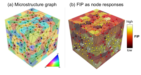
To leverage GNNs for modeling FIPs, we create a microstructure graph for each MVE in the dataset. In the microstructure graph, grains are represented by graph nodes, while grain boundaries are represented by graph edges that link nodes corresponding to spatially adjacent grains (Figure 5a). The MVEs in the dataset are periodic so that the construction of the graphs needs to account for the microstructure periodicity. Specifically, nodes that represent grains on one side of the MVE need to be connected to the nodes representing grain neighbors on the opposite side ($A$–$B$ and $C$–$D$ node pairs in Figure 5a). Furthermore, when a grain is cut by a side of the MVE and thus its part appears on the opposite side, the grain needs to be represented by a single node in the graph. To satisfy the continuity of the microstructure in the graphs of periodic MVEs, we adopt a simple method that duplicates the given MVE and appends its dummy copies to all the six faces of the original MVE. Once we have the MVE augmented with dummy copies, we identify grain neighbors using the DREAM.3D software [37]. From the grain neighbor data, we finally construct a graph with the NetworkX library [38].

We then introduce grain-level properties as node features into the constructed microstructure graphs. We tested two orientation representations: (i) Euler angles, and (ii) quaternions. The MVE dataset that we adopted had triplets of Euler angles in radians as the raw orientation data, which can be readily used as three-element feature vectors. For quaternions as features, we converted the Euler angles into rotation matrices from which we then calculated the four-element quaternion vectors [39]. We further considered Schmid factors of individual grains in respect to the loading direction. Schmid factors quantify resolved shear stresses on each slip system that ultimately drive the dislocation glide in individual grains [40]. For each node in the microstructure graph, we thus assigned 12 Schmid factors calculated for the 12 slip systems in aluminum in respect to the loading direction in the CPFE simulations.

In addition to “input” features, we introduced grain-level FIP values as a response variable for inference at each node (Figure 5b). Following the calculation method by Przyblyla et al. [10], we determined the grain-wise FIP by averaging the maximum FIP values over all integration points of each grain. At each integration point, the maximum FIP is found among all slip systems calculated in CPFE [31] according to Equation 1. The grain-average FIP values are the node properties modeled by the FIP-GNNs developed in this study.

GNN architecture design, optimization, and training

The GNN architecture considered in this study contained message passing layers and a final output layer as the key components of the architecture. A message passing layer aggregates graph node features from first-order nearest neighbors [41] using an aggregation or convolution function. Stacking $k$ message passing layers results in aggregation of features from $k^{\text{th}}$ order neighbors. We considered multiple convolution methods, including SAGE [35], GCN [42], and GIN [43]. Among these methods, SAGE convolution demonstrated significantly better performance in terms of validation error, and was therefore chosen. SAGE convolution includes hidden layers with $n$ neural nodes that process features of each graph node. We treated the number of message passing layers, $k$, the number of neural nodes in the hidden layer, $n$, as well as learning parameters (optimizer, rate, decay, number of warm-up steps) as the main hyperparameters that we optimized to our data.

Figure 6: Simplified illustration of the architecture of FIP-GNN comprised including the input graph, $k$ message passing layers (featuring SAGE convolution with $n$ neural nodes in the hidden layer), and output graph with FIPs as node responses.

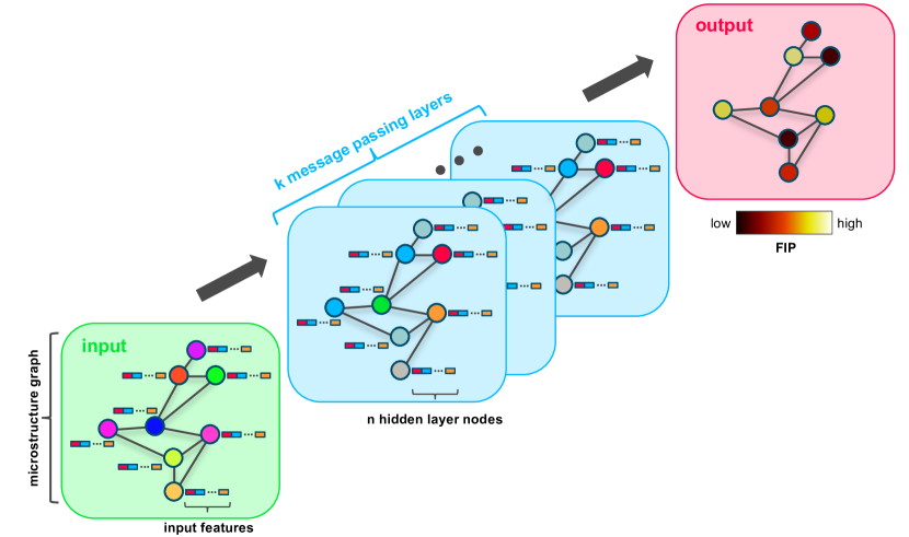
To ensure generalization capability of GNNs to large MVEs, we trained the models and optimized their hyperparameters using only a set of 200 MVEs of the smallest size – MVE30. For hyperparameter optimization, we randomly split the set of 200 MVE30 into training (MVE30-TRAIN) and validation (MVE30-VAL) sets in the $90:10$ ratio. Using validation error as the optimization metric, we found that the convolution method, number of message passing layers, $k$, and the number of hidden layers, $n$, had the biggest impact on the GNN training outcome. SAGE convolution was found the best among the tested three methods, while the optimal combinations of the $k$ and $n$ parameters depended on the selected node features (orientations vs. Shcmid factors) as summarized in Figure 2. Figure 3a further shows the effect of $k$ and $n$ on the mean squared error for the validation set (MVE30-VAL).

References

- [1] J. Miao, T. M. Pollock, J. W. Jones, Crystallographic fatigue crack initiation in nickel-based superalloy rené 88dt at elevated temperature, Acta Materialia 57 (20) (2009) 5964–5974.
- [2] D. L. McDowell, Basic issues in the mechanics of high cycle metal fatigue, International Journal of Fracture 80 (1989) 103–145.
- [3] D. L. McDowell, F. P. Dunne, Microstructure-sensitive computational modeling of fatigue crack formation, International Journal of Fatigue 32 (2010) 1521–1542.
- [4] A. Rovinelli, Y. Guilhem, H. Proudhon, R. A. Lebensohn, W. Ludwig, M. D. Sangid, Assessing reliability of fatigue indicator parameters for small crack growth via a probabilistic framework, Modelling and Simulation in Materials Science and Engineering 25 (4) (2017) 045010.
- [5] G. I. Barenblatt, On a model of small fatigue cracks, Engineering Fracture Mechanics 28 (1987) 623–626.
- [6] F. O. Riemelmoser, R. Pippan, H. P. Stüwe, A comparison of a discrete dislocation model and a continuous description of cyclic crack tip plasticity, International Journal of Fracture 85 (1997) 157–168.
- [7] S. T. Rolfe, J. M. Barsom, Fracture and fatigue control in structures: Applications of fracture mechanics, ASTM International, 1977.
- [8] A. Fatemi, P. Kurath, Multiaxial fatigue life predictions under the influence of mean-stresses, Journal of Engineering Materials and Technology 110 (1988) 380–388.
- [9] G. M. Castelluccio, D. L. McDowell, G. M. Castelluccio, D. L. McDowell, Assessment of small fatigue crack growth driving forces in single crystals with and without slip bands, SpringerGM Castelluccio, DL McDowellInternational journal of fracture, 2012 Springer 176 (2012) 49–64.
- [10] C. P. Przybyla, D. L. McDowell, Microstructure-sensitive extreme value probabilities for high cycle fatigue of ni-base superalloy in100, International Journal of Plasticity 26 (2010) 372–394.
- [11] M. Yaghoobi, K. S. Stopka, A. Lakshmanan, V. Sundararaghavan, J. E. Allison, D. L. McDowell, PRISMS-Fatigue computational framework for fatigue analysis in polycrystalline metals and alloys, npj Computational Materials 2021 7:1 7 (2021) 1–12.
- [12] T. Gu, K. S. Stopka, C. Xu, D. L. McDowell, Modeling the statistical distribution of fatigue crack formation lifetime in large volumes of polycrystalline microstructures, Acta Materialia 247 (2023) 118715.
- [13] M. W. Priddy, N. H. Paulson, S. R. Kalidindi, D. L. McDowell, Strategies for rapid parametric assessment of microstructure-sensitive fatigue for hcp polycrystals, International Journal of Fatigue 104 (2017) 231–242.
- [14] N. H. Paulson, M. W. Priddy, D. L. McDowell, S. R. Kalidindi, Data-driven reduced-order models for rank-ordering the high cycle fatigue performance of polycrystalline microstructures, Materials & Design 154 (2018) 170–183.
- [15] M. I. Latypov, L. S. Toth, S. R. Kalidindi, Materials knowledge system for nonlinear composites, Computer Methods in Applied Mechanics and Engineering 346 (2019) 180–196.
- [16] N. H. Paulson, M. W. Priddy, D. L. McDowell, S. R. Kalidindi, Reduced-order structure-property linkages for polycrystalline microstructures based on 2-point statistics, Acta Materialia 129 (2017) 428–438.
- [17] A. Pandey, R. Pokharel, Machine learning based surrogate modeling approach for mapping crystal deformation in three dimensions, Scripta Materialia 193 (2021) 1–5.
- [18] O. Ibragimova, A. Brahme, W. Muhammad, D. Connolly, J. Lévesque, K. Inal, A convolutional neural network based crystal plasticity finite element framework to predict localised deformation in metals, International Journal of Plasticity 157 (2022) 103374.
- [19] N. N. Vlassis, R. Ma, W. Sun, Geometric deep learning for computational mechanics part i: Anisotropic hyperelasticity, Computer Methods in Applied Mechanics and Engineering 371 (2020) 113299.
- [20] D. C. Pagan, C. R. Pash, A. R. Benson, M. P. Kasemer, Graph neural network modeling of grain-scale anisotropic elastic behavior using simulated and measured microscale data, npj Computational Materials 8 (1) (2022) 259.
- [21] E. Sadeghpour, A. Nonn, Data-driven models for structure-property prediction in additively manufactured steels, Computational Materials Science 215 (2022) 111782.
- [22] J. M. Hestroffer, M.-A. Charpagne, M. I. Latypov, I. J. Beyerlein, Graph neural networks for efficient learning of mechanical properties of polycrystals, Computational Materials Science 217 (2023) 111894.
- [23] A. Thomas, A. R. Durmaz, M. Alam, P. Gumbsch, H. Sack, C. Eberl, Materials fatigue prediction using graph neural networks on microstructure representations, Scientific Reports 2023 13:1 13 (2023) 1–16.
- [24] K. Karimi, H. Salmenjoki, K. Mulewska, L. Kurpaska, A. Kosińska, M. J. Alava, S. Papanikolaou, Prediction of steel nanohardness by using graph neural networks on surface polycrystallinity maps, Scripta Materialia 234 (2023) 115559.
- [25] G. Hu, M. I. Latypov, AnisoGNN: Graph neural networks generalizing to anisotropic properties of polycrystals, Computational Materials Science 243 (2024) 113121. arXiv:2401.16271.
- [26] M. Dai, M. F. Demirel, Y. Liang, J.-M. Hu, Graph neural networks for an accurate and interpretable prediction of the properties of polycrystalline materials, npj Computational Materials 7 (1) (2021) 103.
- [27] Z. Yang, M. J. Buehler, Linking atomic structural defects to mesoscale properties in crystalline solids using graph neural networks, npj Computational Materials 2022 8:1 8 (2022) 1–13.
- [28] M. Dai, M. F. Demirel, X. Liu, Y. Liang, J. M. Hu, Graph neural network for predicting the effective properties of polycrystalline materials: A comprehensive analysis, Computational Materials Science 230 (2023) 112461.
- [29] Y. Hu, G. Zhou, M.-G. Lee, P. Wu, D. Li, A temporal graph neural network for cross-scale modelling of polycrystals considering microstructure interaction, International Journal of Plasticity 179 (2024) 104017.
- [30] A. Frankel, K. Tachida, R. Jones, Prediction of the evolution of the stress field of polycrystals undergoing elastic-plastic deformation with a hybrid neural network model, Machine Learning: Science and Technology 1 (2020) 035005.
-
[31]
K. S. Stopka, M. Yaghoobi, Dataset: PRISMS-Fatigue: predicting distributions of fatigue indicator parameters (2022).
URL https://materialscommons.org/public/datasets/248 - [32] K. S. Stopka, M. Yaghoobi, J. E. Allison, D. L. McDowell, Simulated effects of sample size and grain neighborhood on the modeling of extreme value fatigue response, Acta Materialia 224 (2022) 117524.
- [33] M. Yaghoobi, K. S. Stopka, D. L. McDowell, L. Graham-Brady, K. Teferra, Effect of sample size on the maximum value distribution of fatigue driving forces in metals and alloys, International Journal of Fatigue 176 (2023) 107853.
- [34] M. Lee, H. Lim, B. Adams, J. Hirth, R. Wagoner, A dislocation density-based single crystal constitutive equation, International Journal of Plasticity 26 (7) (2010) 925–938.
- [35] W. L. Hamilton, R. Ying, J. Leskovec, Inductive representation learning on large graphs, NIPS.
- [36] I. Farmaga, P. Shmigelskyi, P. Spiewak, L. Ciupinski, Evaluation of computational complexity of finite element analysis, in: 2011 11th International Conference The Experience of Designing and Application of CAD Systems in Microelectronics (CADSM), 2011, pp. 213–214.
- [37] M. A. Groeber, M. A. Jackson, DREAM.3D: A digital representation environment for the analysis of microstructure in 3D, Integrating Materials and Manufacturing Innovation 3 (1) (2014) 56–72.
- [38] A. Hagberg, P. J. Swart, D. A. Schult, Exploring network structure, dynamics, and function using networkx, Tech. rep., Los Alamos National Laboratory (LANL), Los Alamos, NM (United States) (2008).
- [39] D. Rowenhorst, A. Rollett, G. Rohrer, M. Groeber, M. Jackson, P. J. Konijnenberg, M. De Graef, Consistent representations of and conversions between 3D rotations, Modelling and Simulation in Materials Science and Engineering 23 (8) (2015) 083501.
- [40] E. Schmid, Beiträge zur physik und metallographie des magnesiums, Zeitschrift für Elektrochemie und angewandte physikalische Chemie 37 (8-9) (1931) 447–459.
- [41] J. Gilmer, S. S. Schoenholz, P. F. Riley, O. Vinyals, G. E. Dahl, Neural message passing for quantum chemistry, CoRR abs/1704.01212. arXiv:1704.01212.
- [42] T. N. Kipf, M. Welling, Semi-supervised classification with graph convolutional networks, CoRR abs/1609.02907. arXiv:1609.02907.
- [43] K. Xu, W. Hu, J. Leskovec, S. Jegelka, How powerful are graph neural networks? (2019). arXiv:1810.00826.