What Can We Learn from State Space Models for Machine Learning on Graphs?

Abstract

Machine learning on graphs has recently found extensive applications across domains. However, the commonly used Message Passing Neural Networks (MPNNs) suffer from limited expressive power and struggle to capture long-range dependencies. Graph transformers offer a strong alternative due to their global attention mechanism, but they come with great computational overheads, especially for large graphs. In recent years, State Space Models (SSMs) have emerged as a compelling approach to replace full attention in transformers to model sequential data. It blends the strengths of RNNs and CNNs, offering a) efficient computation, b) the ability to capture long-range dependencies, and c) good generalization across sequences of various lengths. However, extending SSMs to graph-structured data presents unique challenges due to the lack of canonical node ordering in graphs. In this work, we propose Graph State Space Convolution (GSSC) as a principled extension of SSMs to graph-structured data. By leveraging global permutation-equivariant set aggregation and factorizable graph kernels that rely on relative node distances as the convolution kernels, GSSC preserves all three advantages of SSMs. We demonstrate the provably stronger expressiveness of GSSC than MPNNs in counting graph substructures and show its effectiveness across 10 real-world, widely used benchmark datasets, where GSSC achieves best results on 7 out of 10 datasets with all significant improvements compared to the state-of-the-art baselines and second-best results on the other 3 datasets. Our findings highlight the potential of GSSC as a powerful and scalable model for graph machine learning. Our code is available at https://github.com/Graph-COM/GSSC.

1 Introduction

Machine learning for graph-structured data has numerous applications in molecular graphs [23, 109], drug discovery [115, 94], and social networks [29, 42]. In recent years, Message Passing Neural Networks (MPNNs) have been arguably one of the most popular neural architectures for graphs [56, 33, 101, 116, 19, 124]. However, it is shown that MPNNs suffer from many limitations, including restricted expressive power [116, 76], over-squashing [21, 98, 77], and over-smoothing [89, 9, 54]. These limitations could potentially harm the model’s performance. For example, MPNNs cannot detect common subgraph structures like cycles that play an important role in forming ring systems of molecular graphs [13], and they also fail to capture long-range dependencies [27].

Adapted from the vanilla transformer in sequence modeling [100], graph transformers have attracted growing research interests because they may alleviate these fundamental limitations of MPNNs [60, 55, 87, 11, 24]. By attending to all nodes in the graph, graph transformers are inherently able to capture long-range dependencies. However, the global attention mechanism ignores graph structures and thus requires incorporating positional information of nodes known as positional encodings (PEs) [87] that encode graph structural information, in particular the information of relative distance between nodes for attention computation [66, 104, 117]. Moreover, the standard full attention scales quadratically with respect to the length of the sequence or the size of the graph to be encoded. This computational limitation motivates the study of linear-time transformers by incorporating techniques such as low-rank [52, 106, 15, 16] or sparse approximations [50, 57, 20, 121, 44] of the full attention matrix for model acceleration. Some specific designs of scalable transformers for large-scale graphs are also proposed [110, 12, 90, 112, 59, 111]. Nevertheless, none of these variants have been proven to be consistently effective across different domains [75].

State Space Models (SSMs) [40, 41, 37] have recently demonstrated promising potentials for sequence modeling. Adapted from the classic state space model [51], SSMs can be seen as a hybrid of recurrent neural networks (RNNs) and convolutional neural networks (CNNs). It is a temporal convolution that preserves translation invariance and thus allows good generalization to longer sequences. Meanwhile, this class of models has been shown to be able to effectively capture long-range dependencies both theoretically and empirically [38, 97, 41, 40]. Finally, it can be efficiently computed in linear or near-linear time via either the recurrence mode or the convolution mode. These advantages make the SSM a strong candidate as an alternative to transformers [73, 71, 31, 105, 95].

Given the great potential of SSMs, there is increasing interest in generalizing them for graphs as an alternative to graph transformers [103, 4]. The main technical challenge is that SSMs are defined on sequences that are ordered and causal, i.e., have a linear structure. Yet, graphs have complex topology, and no canonical node ordering can be found. Naive tokenization (e.g., sorting nodes into a sequence in some way) breaks the inductive bias - permutation symmetry - of graphs, which consequently may not faithfully represent graph topology and could suffer from a poor generalization capability.

In this study, we go back to the fundamental question of how to properly define SSMs in the graph space. Instead of simply tokenizing graphs and directly applying existing SSMs for sequences (which may break the symmetry), we argue that principled graph SSMs should inherit the advantages of SSMs in capturing long-range dependencies and being efficient. Simultaneously, they should also preserve the permutation symmetry of graphs to achieve good generalization. Therefore, in this work:

• We identify that the key component enabling SSMs for sequences to be long-range, efficient, and well-generalized to longer sequences, is the use of a global, factorizable, and translation-invariant kernel that depends on relative distances between tokens. This relative-distance kernel can be factorized into the product of absolute positions, crucial to achieving linear-time complexity.

• This observation motivates us to design Graph State Space Convolution (GSSC) in the following way: (1) it leverages a global permutation equivariant set aggregation that incorporates all nodes in the graph; (2) the aggregation weights of set elements rely on relative distances between nodes on the graph, which can be factorized into the "absolute positions" of the corresponding nodes, i.e., the PEs of nodes. By design, the resulting GSSC is inherently permutation equivariant, long-range, and linear-time. Besides, we also demonstrate that GSSC is more powerful than MPNNs and can provably count at least $4$-paths and $4$-cycles.

• Empirically, our experiments demonstrate the high expressivity of GSSC via graph substructure counting and validate its capability of capturing long-range dependencies on Long Range Graph Benchmark [27]. Results on 10 real-world, widely used graph machine learning benchmark datasets [46, 25, 27] also show the consistently superior performance of GSSC, where GSSC achieves best results on 7 out of 10 datasets with all significant improvements compared to the state-of-the-art baselines and second-best results on the other 3 datasets. Moreover, it has much better scalability than the standard graph transformers in terms of training and inference time.

2 Related Works

Graph Neural Networks (GNNs) and Graph Transformers. Most GNNs adopt a message-passing mechanism that aggregates information from neighboring nodes and integrates it into a new node representation [56, 116, 19, 101]. However, these models are shown to be no more expressive than 1-WL test, a classic graph isomorphism test algorithm [116, 76], and they could suffer from over-smoothing and over-squashing issues and are unable to capture long-range dependencies [2, 98]. On the other hand, graph transformers leverage attention mechanism [100, 24, 60, 55, 11] that can attend to all nodes in a graph. As full attention ignores graph topology and makes nodes indistinguishable, many works focus on designing effective positional encodings or distance encodings (relative positional encodings) of nodes, e.g., Laplacian positional encodings [25, 60, 72, 26, 104, 68, 47, 55], shortest path distance [66, 118], diffusion/random walk distance [74], gradients of Laplacian eigenvectors [3], etc. Another type of method combines MPNNs with full attention [87, 10]. Yet, the full attention scales quadratically to graph size. To reduce such complexity, [87] adopts general linear attention techniques [16, 120] to graph transformers, and some techniques specifically designed for graph transformers are also proposed [110, 12, 90, 112, 59, 111].

State Space Models (SSMs). Classic SSMs [51, 49, 22] describe the evolution of state variables over time using first-order differential equations or difference equations, providing a unified framework for time series modeling. Similar to RNNs [82, 36, 96], SSMs may also suffer from poor memorization of long contexts and long-range dependencies. To address this issue, [38] proposes a principled framework to introduce long-range dependencies for SSMs. To solve the computational bottleneck of SSMs, a series of works named Structural SSM (S4) [40, 92, 43, 39] are developed to leverage special structures (e.g., diagonal structures) of parameter matrices to speed up matrix multiplications. [71] proposes a simplified variant of S4 in real domain. [45] augments S4 with data-dependent state transition. [85, 67, 32, 86] can be interpreted as S4 with different parameterizations of global convolutional kernels. [37] introduces a selective mechanism to make the SSM’s transition data-dependent. The development of SSMs also inspires a new class of neural architectures as a hybrid of SSMs and other deep learning models [73, 71, 31]. There are also works that can be interpreted from the perspective of SSMs [83, 95]. See [107] for a comprehensive survey.

State Space Models for Graphs. There are some efforts to replace the attention mechanism in graph transformers with SSMs. They mainly focus on tokenizing graphs and apply the existing SSM — Mamba [37]. Graph-Mamba-I [103] sorts nodes into sequences by node degrees and applies Mamba. As node degrees can have multiplicity, this approach requires random permutation of sequences during training, and the resulting model is not permutation equivariant to node indices reordering. For Graph-Mamba-II [5], it extracts the $1,2,...,M$-hop neighborhood of a root node, treats each hop of the neighborhood as a token, and applies Mamba to the sequence of neighborhoods to obtain the representation of the root node. This approach incurs significant computational overhead as it requires applying a GNN to encode every neighborhood token first. In the last layer, it additionally applies Mamba to nodes sorted by node degrees, making it not permutation equivariant as well.

3 Preliminaries

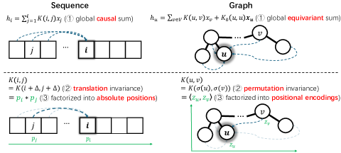
Figure 1: Comparison of Sequence State Space Conv. (left) and Graph State Space Conv. (right).

Graphs and Graph Laplacian. Let $\mathcal{G}=(\mathcal{V},\mathcal{E})$ be a undirected graph, where $\mathcal{V}$ is the node set and $\mathcal{E}$ is the edge set. Suppose $\mathcal{G}$ has $n$ nodes. Let $\bm{A}\in\mathbb{R}^{n\times n}$ be the adjacency matrix of $\mathcal{G}$ and $\bm{D}=\text{diag}([\sum_{j}\bm{A}_{1,j},...,\sum_{j}\bm{A}_{n,j}])$ be the diagonal degree matrix. The (normalized) graph Laplacian is defined by $\bm{L}=\bm{I}-\bm{D}^{-1/2}\bm{A}\bm{D}^{-1/2}$ where $\bm{I}$ is the $n$ by $n$ identity matrix.

State Space Models. State space model is a continuous system that maps a input function $x(t)$ to output $h(t)$ by the following first-order differential equation: $\frac{d}{dt}h(t)=Ax(t)+Bx(t).$ This system can be discretized by applying a discretization rule (e.g., bilinear method [99], zero-order hold [37]) with time step $\Delta$. Suppose $h_{i}:=h(i\cdot\Delta)$ and $x_{i}:=x(i\cdot\Delta)$. The discrete state space model becomes a recurrence process:

$$h_{i}=\bar{A}h_{i-1}+\bar{B}x_{i},$$ (1)

where $\bar{A}=f_{A}(\Delta,A)$ and $\bar{B}=f_{B}(\Delta,B)$ depend on the specific discretization rule. The recurrence Eq. (1) can be computed equivalently by a global convolution:

$$h_{i}=\sum_{j=1}^{i}\bar{A}^{i-j}\bar{B}x_{j}.$$ (2)

In the remaining of this paper, we call convolution Eq. (2) state space convolution (SSC). Notably, the state space model enjoys three key advantages simultaneously:

• Translation equivariance. A translation to input $x_{i}\to x_{i+\delta}$ yields the same translation to output $h_{i}\to h_{i+\delta}$.

• Long-range dependencies. The feature $h_{i}$ of $i$-th token depends on all preceding tokens’ features $x_{1},x_{2},...,x_{i-1}$, instead of those in a fixed size receptive field as traditional CNNs [64, 61].

• Computational efficiency and parallelism. To computing $h_{1},h_{2},...,h_{n}$, it either uses linear-time recurrence (Eq. 1) or parallelizable convolution (Eq. 2).

Notation. Suppose $x,y$ are two vectors of dimension $n$. Denote $\langle x,y\rangle=\sum_{i=1}^{n}x_{i}y_{i}$ as the inner product, $x\odot y=(x_{1}y_{1},x_{2}y_{2},...)$ be the element-wise product. We generally denote the hidden dimension by $m$, and the dimension of positional encodings by $d$.

4 Graph State Space Convolution

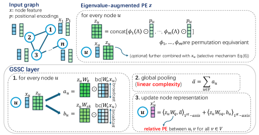
Figure 2: Illustration of Graph State Space Convolution (GSSC).

4.1 Generalizing State Space Convolution to Graphs

The desired graph SSC should keep the advantages of the standard SSC (Eq. $\eqref{ssm-convolution}$) regarding the capabilities of capturing long-range dependencies while maintaining linear-time complexity and parallelizability. Meanwhile, permutation equivariance as a strong inductive bias of graph-structured data should be preserved by the model as well to improve generalization.

Our key observations of SSC (Eq. $\eqref{ssm-convolution}$) start with the fact that the convolution kernel $\bar{A}^{i-j}$ encoding the relative distance $i-j$ between token $i$ and $j$ allows for a natural factorization:

$$h_{i}=\sum_{j=1}^{i}\bar{A}^{i-j}\bar{B}x_{j}=\bar{A}^{i}\sum_{j=1}^{i}\bar{A}^{-j}\bar{B}x_{j}.$$ (3)

Generally, a sum $\sum_{j}K(i,j)x_{j}$ with a generic kernel $K(i,j)$ requires quadratic-time complexity and may not capture translation invariant patterns for variable-length generalization. For SSC (Eq. (3)), however, it captures translation invariant patterns by adopting a translation-invariant kernel $K(i-j)$ that only depends on the relative distance $i-j$, which gives the generalization power to sequences even longer than those used for training [34, 53]. Moreover, SSC attains computational efficiency by leveraging the factorability of its particular choice of the relative distance kernel $K(i-j)=\bar{A}^{i-j}=\bar{A}^{i}\cdot\bar{A}^{-j}$, where the two factors only depend on the absolute positions of token $i$ and $j$ respectively. Specifically, to compute $h$, one may construct $[\sum_{j=1}^{1}\bar{A}^{-j}\bar{B}x_{j},...,\sum_{j=1}^{n}\bar{A}^{-j}\bar{B}x_{j}]$ using prefix sum with complexity $O(n)$, and then readout $h_{i}$ by multiplying $\bar{A}^{i}$ for all $i=1,2,...,n$ in parallel with complexity $O(n)$. Finally, its use of the global sum pooling operation over $j$ instead of small-window convolution kernels commonly used in CNNs [62] is the key to capturing global dependencies. Overall, the advantages of SSC are attributed to these three aspects.

Inspired by these insights, a natural generalization of SSC to graphs should adopt permutation-invariant kernels $K(v,u)$, $v,u\in\mathcal{V}$ due to the inductive bias from sequences to graphs, which are also factorizable $K(v,u)=z_{v}^{\top}z_{u}$, and the convolution should be performed global pooling across the entire graph to capture global dependences.

Fortunately, a systematic strategy can be adopted to achieve the goal. First, the kernel $K(v,u)$ can be defined to depend on some notations of relative distance between nodes to keep permutation invariance. The choices include but are not limited to shortest-path distance, random walk landing probability [65] (such as PageRank [79, 35]), heat (diffusion) distance [18], resistance distance [114, 81], bi-harmonic distance [69], etc. Many of them have been widely adopted as edge features for existing models, e.g., GNNs [119, 66, 122, 14, 102, 78] and graph transformers [60, 87, 70, 74]. More importantly, all these kernels can be factorized into some weighted inner product of Laplacian eigenvectors [6]. Here, Laplacian eigenvectors, also known as Laplacian positional encodings [25], play the role of the absolute positions of nodes in the graph. Formally, consider the eigendecomposition $\bm{L}=\bm{V}\bm{\Lambda}\bm{V}^{\top}$ and let $p_{u}=[\bm{V}_{u,:}]^{\top}$ be Laplacian positional encodings for node $u$. Then a relative-distance kernel $K(u,v)$ can be generally factorized into $K(u,v)=p_{u}^{\top}(\phi(\bm{\Lambda})\odot p_{v})$ for a certain function $\phi$. For instance, diffusion kernel satisfies $[\phi(\bm{\Lambda})]_{k}=\exp(-t\lambda_{k})$ for some time parameter $t$. Due to factorization, one may achieve global sum aggregation via $O(n)$ complexity. For the potential super-linear complexity to compute such factorization, we leave the discussion in Sec. 4.2.

Graph State Space Convolution (GSSC). Given the above observations, we propose GSSC as follows. Given the input node features $x_{u}\in\mathbb{R}^{m}$, the $d$-dim Laplacian positional encodings $p_{u}=[\bm{V}_{u,1:d}]^{\top}\in\mathbb{R}^{d}$, and the corresponding $d$ eigenvalues $\bm{\Lambda}_{d}=[\lambda_{1},...,\lambda_{d}]^{\top}$, then, the output node representations $h_{u}\in\mathbb{R}^{m}$ follow

$$h_{u} =\sum_{v\in\mathcal{V}}\langle z_{u}\bm{W}_{q},z_{v}\bm{W}_{k}\rangle\odot\bm{W}_{o}x_{v}+\langle z_{u}\bm{W}_{sq},z_{u}\bm{W}_{sk}\rangle\odot\bm{W}_{s}x_{u},$$ (4)

$$=\langle z_{u}\bm{W}_{q},(\sum_{v\in\mathcal{V}}z_{v}\bm{W}_{k})\odot\bm{W}_{o}x_{v}\rangle+\langle z_{u}\bm{W}_{sq},z_{u}\bm{W}_{sk}\odot\bm{W}_{s}x_{u}\rangle.$$ (5)

Here $z_{u}=[\phi_{1}(\bm{\Lambda}_{d})\odot p_{u},...,\phi_{m}(\bm{\Lambda}_{d})\odot p_{u}]\in\mathbb{R}^{d\times m}$ represents the eigenvalue-augmented positional encodings from raw $d$-dim positional encodings $p_{u}$ and $\phi_{\ell}:\mathbb{R}^{d}\to\mathbb{R}^{d}$ are learnable permutation equivariant functions w.r.t. $d$-dim axis (i.e., equivariant to permutation of eigenvalues). All $\bm{W}\in\mathbb{R}^{m\times m}$ with different subscripts are learnable weight matrices. The inner product $\langle z_{u}\bm{W}_{q},z_{v}\bm{W}_{k}\rangle\in\mathbb{R}^{m}$ only sums over the first $d$-dim axis and produces a $m$-dim vector. The term $z_{u}\bm{W}_{sk}\odot\bm{W}_{s}x_{u}$ in Eq.(5) should be interpreted as first broadcasting $\bm{W}_{s}x_{u}$ from $\mathbb{R}^{m}$ to $\mathbb{R}^{d\times m}$ and then performing element-wise products. Note that Eqs. (4),(5) is a generalization of SSC Eq. (3) in the sense that:

• The product of absolute position $\bar{A}^{i}\bar{A}^{-j}$ is replaced by the inner product of graph positional encodings $\langle z_{u}\bm{W}_{q},z_{v}\bm{W}_{k}\rangle$.

• $\sum_{j=1}^{i}\bar{A}^{-j}\bar{B}x_{j}$ aggregates token’s features in a causal way, i.e., from the start token to itself. As graphs are not causal, a node $u$ only distinguishes itself (node $u$) from other nodes. So we adopt permutation equivariant global pooling $z_{u}\bm{W}_{sk}\odot\bm{W}_{s}x_{u}$ including node $i$ itself, and $(\sum_{v\in\mathcal{V}}z_{v}\bm{W}_{k})\odot\bm{W}_{o}x_{v}$ including all nodes in the graph.

Remark 4.1.

Graph state space convolution (Eq. (4),(5)) is (1) permutation equivariant: a permutation of node indices reorders $h_{i}$ correspondingly; (2) long-range: node features $h_{i}$ depends on all nodes in the graph; (3) linear-time: the complexity of computing $h_{1},...,h_{n}$ from $x_{1},...,x_{n}$ is $\mathcal{O}(nmd)$; (4) stable: perturbation to graph Laplacian yields a controllable change of GSSC model output, because permutation equivariance and smoothness of $\phi_{\ell}$ ensure the stability of inner product $\langle z_{u}\bm{W}_{q},z_{v}\bm{W}_{k}\rangle$ and model output, as shown in [104, 47]. Stability is an enhanced concept of permutation equivariance and is crucial for out-of-distribution generalization [47].

4.2 Further Extensions and Discussions

Incorporating Edge Features. GSSC (Eq.(4)) refines node features based on graph structures. To further incorporate edge features, we can leverage MPNNs that can introduce edge features in the message-passing mechanism. In practice, we adopt the framework of GraphGPS [87]: In each layer, node representations are passed both into an MPNN layer and a GSSC layer, and the two outputs are added into a new representation. Here GSSC replaces the role of vanilla transformer in GraphGPS.

Selection Mechanism in SSMs. It is known that SSMs lack of selection mechanism, i.e., the kernel $\bar{A}^{i-j}$ is only a function of positions $i,j$ and does not rely on the feature of tokens [37]. To improve the content-aware ability of SSMs, Gu & Dao [37] proposed to make coefficients $\bar{A},\bar{B}$ in Eq.(1) data-dependent, i.e., replacing $\bar{A}$ by $\bar{A}_{i}:=\bar{A}(x_{i})$ and $\bar{B}$ by $\bar{B}_{i}:=\bar{B}(x_{i})$. This leads to a data-dependent convolution: $h_{i}=\sum_{j=1}^{i}\bar{A}_{i-1}\bar{A}_{i-2}...\bar{A}_{j}\bar{B}_{j}x_{j}$. Again, this convolution can be factorized into $h_{i}=\tilde{A}_{i}(\sum_{j=1}^{i}\tilde{A}_{j}\bar{B}_{j}x_{j})$, where $\tilde{A}_{i}:=\bar{A}_{i-1}\bar{A}_{i-2}...\bar{A}_{1}$ can be interpreted as a data-dependent absolute position of token $i$, depending on features and positions of all preceding tokens. We can generalize this “data-dependent position” idea to GSSM, defining a data-dependent positional encodings $\tilde{z}$ as follows:

$$\tilde{z}_{u}=\sum_{v\in\mathcal{V}}\langle z_{u}\bm{W}_{dq},z_{v}\bm{W}_{dk}\rangle(z_{u}\odot x_{u})\bm{W}_{dv},$$ (6)

where $z_{u}\odot x_{u}$ should be interpreted as first broadcasting $x_{u}$ from $\mathbb{R}^{m}$ to $\mathbb{R}^{r\times m}$ and then doing the element-wise product with $z_{u}$. Note that the new positional encodings $\tilde{z}_{u}$ reply on the features and positional encodings of all nodes, which reflects permutation equivariance. To achieve a selection mechanism, we can replace every $z_{u}$ in Eqs.(4) by $\tilde{z}_{u}$. Thanks to the factorizable kernel $\langle z_{u}\bm{W}_{dq},z_{v}\bm{W}_{dk}\rangle$, computing $\tilde{z}_{u}$ can still be done in $\mathcal{O}(nmd^{2})$, linear w.r.t. graph size.

Compared to Graph Spectral Convolution (GSC). The convolution (Eq. (4)) may remind us of the graph spectral convolution, which is usually in the form of $\bm{H}=\bm{V}\psi(\bm{\Lambda})\bm{V}^{\top}\bm{X}\bm{W}$, where $\bm{H}=[h_{1}^{\top};...;h_{n}^{\top}]^{\top}\in\mathbb{R}^{n\times m}$ and $\bm{X}=[x_{1}^{\top};...;x_{n}^{\top}]^{\top}\in\mathbb{R}^{n\times m}$ are a row-wise concatenation of features, $\psi(\bm{\Lambda})=\text{diag}([\psi(\lambda_{1}),...,\psi(\lambda_{n})])$ is the spectrum-domain filtering with $\psi:\mathbb{R}\to\mathbb{R}$ usually being a polynomial function. Equivalently, it can be written as $h_{u}=\sum_{v\in\mathcal{V}}\langle p_{u},\psi(\bm{\Lambda})\odot p_{v}\rangle\bm{W}x_{v}$. There are several differences between GSSC (Eq. $\eqref{gssm}$) and graph spectral convolution: 1) $\psi:\mathbb{R}\to\mathbb{R}$ is typically an element-wise polynomial filters for spectral convolution, while $\phi:\mathbb{R}^{m}\to\mathbb{R}^{m}$ is a general permutation equivariant function that can jointly leverage the spectrum information; 2) GSSC distinguishes a node itself (weight $\bm{W}_{sq},\bm{W}_{sk},\bm{W}_{so}$) and other nodes (weight $\bm{W}_{q},\bm{W}_{k},\bm{W}_{o}$) via a permutation equivariant layer, while GSC treats all nodes using the same weight $\bm{W}$. The former can, for example, consider only self-features by letting $\bm{W}_{o}=0$ while the latter cannot do so. This function of excluding other nodes turns out to be helpful to express the diagonal element extraction ($\text{diag}(\bm{A}^{k})$) to perform cycle counting. In comparison, GSC with non-distinguishable node features cannot be more powerful than 1-WL test [108], while GSSC, as shown later is more powerful.

Super-linear Computation of Laplacian Eigendecomposition. GSSC requires the computation of Laplacian eigendecomposition as preprocessing. Although finding all eigenvectors and eigenvalues can be costly, (1) in real experiments, such preprocessing can be done efficiently, which may only occupy less than 10% wall-clock time of the entire training process (see Sec. 5.3 for quantitative results on real-world datasets); (2) we only need top-$d$ eigenvectors and eigenvalues, which can be efficiently found by Lanczos methods [80, 63] with complexity $O(nd^{2})$ or similarly by LOBPCG methods [58]; (3) one can also adopt random Fourier feature-based approaches to fast approximate those kernels’ factorization [93, 17, 88] without precisely computing the eigenvectors.

4.3 Expressive Power

We study the expressive power of GSSC via the ability to count graph substructures. The following theorem states that GSSC (4) can count at least 3-paths and 3-cycles, which is strictly stronger than MPNNs and GSC (both cannot count 3-cycles [13, 108]). Furthermore, if we introduce the selection mechanism Eq. (6), it can provably count at least $4$-paths and $4$-cycles.

Theorem 4.1 (Counting paths and cycles).

Graph state space convolution Eq. (4) can at least count number of $3$-paths and $3$-cycles. With selection mechanism Eq. (6), it can at least count number of $4$-paths and $4$-cycles. Here “counting” means the node representations can express the number of paths starting at the node or number of cycles involving the node.

5 Experiments

Table 1: Benchmark on GNN Benchmark & Long Range Graph Benchmark. $\textbf{Bold}^{\dagger}$, $\textbf{Bold}^{\ddagger}$, and Bold denote the first, second, and third best results, respectively. Results are reported as $\text{mean}_{\pm\text{std}}$.

	MNIST	CIFAR10	PATTERN	CLUSTER	PascalVOC-SP	Peptides-func	Peptides-struct
	Accuracy $\uparrow$	Accuracy $\uparrow$	Accuracy $\uparrow$	Accuracy $\uparrow$	F1 score$\uparrow$	AP $\uparrow$	MAE $\downarrow$
GCN	$90.705_{\pm 0.218}$	$55.710_{\pm 0.381}$	$71.892_{\pm 0.334}$	$68.498_{\pm 0.976}$	$0.1268_{\pm 0.0060}$	$0.5930_{\pm 0.0023}$	$0.3496_{\pm 0.0013}$
GIN	$96.485_{\pm 0.252}$	$55.255_{\pm 1.527}$	$85.387_{\pm 0.136}$	$64.716_{\pm 1.553}$	$0.1265_{\pm 0.0076}$	$0.5498_{\pm 0.0079}$	$0.3547_{\pm 0.0045}$
GAT	$95.535_{\pm 0.205}$	$64.223_{\pm 0.455}$	$78.271_{\pm 0.186}$	$70.587_{\pm 0.447}$	$-$	$-$	$-$
GatedGCN	$97.340_{\pm 0.143}$	$67.312_{\pm 0.311}$	$85.568_{\pm 0.088}$	$73.840_{\pm 0.326}$	$0.2873_{\pm 0.0219}$	$0.5864_{\pm 0.0077}$	$0.3420_{\pm 0.0013}$
SAN	$-$	$-$	$86.581_{\pm 0.037}$	$76.691_{\pm 0.650}$	$0.3216_{\pm 0.0027}$	$0.6439_{\pm 0.0075}$	$0.2545_{\pm 0.0012}$
GraphGPS	$98.051_{\pm 0.126}$	$72.298_{\pm 0.356}$	$86.685_{\pm 0.059}$	$78.016_{\pm 0.180}$	$0.3748_{\pm 0.0109}$	$0.6535_{\pm 0.0041}$	$0.2500_{\pm 0.0005}$
Exphormer	$\mathbf{98.550}^{\dagger}_{\pm 0.039}$	$\mathbf{74.690}_{\pm 0.125}$	$\mathbf{86.740}_{\pm 0.015}$	$\mathbf{78.070}_{\pm 0.037}$	$\mathbf{0.3975}_{\pm 0.0037}$	$0.6527_{\pm 0.0043}$	$0.2481_{\pm 0.0007}$
Grit	$98.108_{\pm 0.111}$	$\mathbf{76.468}^{\ddagger}_{\pm 0.881}$	$\mathbf{87.196}^{\ddagger}_{\pm 0.076}$	$\mathbf{80.026}^{\dagger}_{\pm 0.277}$	$-$	$\mathbf{0.6988}^{\ddagger}_{\pm 0.0082}$	$\mathbf{0.2460}^{\ddagger}_{\pm 0.0012}$
Graph-Mamba-I	$\mathbf{98.420}_{\pm 0.080}$	$73.700_{\pm 0.340}$	$86.710_{\pm 0.050}$	$76.800_{\pm 0.360}$	$\mathbf{0.4191}^{\ddagger}_{\pm 0.0126}$	$\mathbf{0.6739}_{\pm 0.0087}$	$\mathbf{0.2478}_{\pm 0.0016}$
GSSC	$\mathbf{98.492}^{\ddagger}_{\pm 0.051}$	$\mathbf{77.642}^{\dagger}_{\pm 0.456}$	$\mathbf{87.510}^{\dagger}_{\pm 0.082}$	$\mathbf{79.156}^{\ddagger}_{\pm 0.152}$	$\mathbf{0.4561}^{\dagger}_{\pm 0.0039}$	$\mathbf{0.7081}^{\dagger}_{\pm 0.0062}$	$\mathbf{0.2459}^{\dagger}_{\pm 0.0020}$

We evaluate the effectiveness of GSSC on 13 datasets against various baselines. Particularly, we focus on answering the following questions:

• Q1: How expressive is GSSC in terms of counting graph substructures?

• Q2: How effectively does GSSC capture long-range dependencies?

• Q3: How does GSSC perform on general graph benchmarks compared to other baselines?

• Q4: How does the computational time/space of GSSC scale with graph size?

Below we briefly introduce the model implementation, included datasets and baselines, and a more detailed description can be found in Appendix B.

Datasets. To answer Q1, we use the graph substructure counting datasets from [13, 123, 48]. Each of the synthetic datasets contains 5k graphs generated from different distributions (see [13] Appendix M.2.1), and the task is to predict the number of cycles as node-level regression. To answer Q2, we evaluate GSSC on Long Range Graph Benchmark [27], which requires long-range interaction reasoning to achieve strong performance. Specifically, we adopt Peptides-func (graph-level classification with 10 functional labels of peptides), Peptides-struct (graph-level regression of 11 structural properties of molecules), and PascalVOC-SP (classify superpixels of image graphs into corresponding object classes). To answer Q3, molecular graph datasets (ZINC [25] and ogbg-molhiv [46]), image graph datasets (MNIST, CIFAR10 [25]) and synthetic graph datasets (PATTERN, CLUSTER [25]) are used to evaluate the performance of GSSC. ZINC is a molecular property prediction (graph regression) task containing two partitions of dataset, ZINC-12K (12k samples) and ZINC-full (250k samples). Ogbg-molhiv consists of 41k molecular graphs for graph classification. CIFAR10 and MNIST are 8-nearest neighbor graph of superpixels constructed from images for classification. PATTERN and CLUSTER are synthetic graphs generated by the Stochastic Block Model (SBM) to perform node-level community classification. Finally, to answer Q4, we construct a synthetic dataset with graph sizes from 1k to 60k to evaluate how GSSC scales.

GSSC Implementation. We implement deep models consisting of GSSC blocks Eq.(4). Each layer includes one MPNN (to incorporate edge features) and one GSSC block, as well as a nonlinear readout to merge the outputs of MPNN and GSSC. The resulting deep model can be seen as a GraphGPS [87] with the vanilla transformer replaced by GSSC. Selective mechanism is excluded in all tasks except cycle-counting datasets, because we find the GSSC w/o selective mechanism is already powerful and yields excellent results in real-world tasks. In our experiments, GSSC utilizes the smallest $d=32$ eigenvalues and their eigenvectors for all datasets except molecular ones, which employ $d=16$. See Appendix B for full details of model hyperparameters.

Baselines. We consider various baselines that can be mainly categorized into: (1) MPNNs: GCN [56], GIN [116], GAT [101], Gated GCN [8] and PNA [19]; (2) Subgraph GNNs: NGNN [122], ID-GNN [119], GIN-AK+ [123], I²-GNN [48]; (3) high-order GNNs: SUN [30]; (4) Graph transformers: Graphormer [117], SAN [60], GraphGPS [87], Exphormer [90], Grit [70]; (5) Others: Specformer [7], Graph-Mamba-I [103], SignNet [68], SPE [47]. Note that we also include the baseline Graph-Mamba-II [4], and GSSC outperforms it on all included datasets, but we put their results in Appendix C as we cannot reproduce their results due to the lack of code.

5.1 Graph Substructure Counting

Table 2: Benchmark on graph substructure counting (normalized MAE $\downarrow$ ).

	$3$-Cycle	$4$-Cycle	$5$-Cycle
GIN	$0.3515$	$0.2742$	$0.2088$
ID-GIN	$0.0006$	$0.0022$	$0.0490$
NGNN	$0.0003$	$0.0013$	$0.0402$
GIN-AK+	$0.0004$	$0.0041$	$0.0133$
I2-GNN	$0.0003$	$0.0016$	$0.0028$
GSSC	$0.0002$	$0.0013$	$0.0113$

Table 2 shows the normalized MAE results (absolute MAE divided by the standard deviation of targets). Here the backbone GNN is GIN for all baseline subgraph models [48]. In terms of predicting $3$-cycles and $4$-cycles, GSSC achieves the best results compared to subgraph GNNs and I²-GNNs, which are models that can provably count $3,4$-cycles, validating Theorem 4.1. For the prediction of $5$-cycles, GSSC greatly outperforms the MPNN and ID-GNN, which are models that cannot predict $5$-cycles, reducing normalized MAE by $94.6\%$ and $71.9\%$, respectively. Besides, GSSC achieves constantly better performance than GNNAK+, a subgraph GNN model that is strictly stronger than ID-GNN and NGNN [48]. These results demonstrate the empirically strong function-fitting ability of GSSC.

5.2 Graph Learning Benchmarks

Table 3: Benchmark on molecular datasets. $\textbf{Bold}^{\dagger}$, $\textbf{Bold}^{\ddagger}$, and Bold denote the first, second, and third best results, respectively.

	ZINC-12k	ZINC-Full	ogbg-molhiv
	MAE $\downarrow$	MAE $\downarrow$	AUROC $\uparrow$
GCN	$0.367_{\pm 0.011}$	$0.113_{\pm 0.002}$	$75.99_{\pm 1.19}$
GIN	$0.526_{\pm 0.051}$	$0.088_{\pm 0.002}$	$77.07_{\pm 1.49}$
GAT	$0.384_{\pm 0.007}$	$0.111_{\pm 0.002}$	$-$
PNA	$0.188_{\pm 0.004}$	$-$	$79.05_{\pm 1.32}$
NGNN	$0.111_{\pm 0.003}$	$0.029_{\pm 0.001}$	$78.34_{\pm 1.86}$
GIN-AK+	$0.080_{\pm 0.001}$	$-$	$\mathbf{79.61}_{\pm 1.19}$
I2-GNN	$0.083_{\pm 0.001}$	$0.023_{\pm 0.001}$	$78.68_{\pm 0.93}$
SUN	$0.083_{\pm 0.003}$	$0.024_{\pm 0.003}$	$\mathbf{80.03}^{\ddagger}_{\pm 0.55}$
Graphormer	$0.122_{\pm 0.006}$	$0.052_{\pm 0.005}$	$-$
SAN	$0.139_{\pm 0.006}$	$-$	$77.85_{\pm 2.47}$
GraphGPS	$0.070_{\pm 0.004}$	$-$	$78.80_{\pm 1.01}$
Specformer	$\mathbf{0.066}_{\pm 0.003}$	$-$	$78.89_{\pm 1.24}$
SPE	$0.070_{\pm 0.004}$	$-$	$-$
SignNet	$0.084_{\pm 0.006}$	$0.024_{\pm 0.003}$	$-$
Grit	$\mathbf{0.059}^{\dagger}_{\pm 0.002}$	$0.023_{\pm 0.001}$	$-$
GSSC	$\mathbf{0.064}^{\ddagger}_{\pm 0.002}$	$\mathbf{0.019}^{\dagger}_{\pm 0.001}$	$\mathbf{80.35}^{\dagger}_{\pm 1.42}$

Table 1 and Table 3 evaluate the performance of GSSC on multiple widely used graph learning benchmarks. GSSC achieves excellent performance on all benchmark datasets, and the result of each benchmark is discussed below.

Long Range Graph Benchmark [27]. We test the ability to model long-range interaction on PascalVOC-SP, Peptides-func and Peptides-struct, as shown in Table 1. Remarkably, GSSC achieves state-of-the-art results on all three datasets. It demonstrates that GSSC is highly capable of capturing long-range dependencies as expected, due to the usage of global permutation equivariant aggregation operations and factorizable relative positional encodings.

Molecular Graph Benchmark [25, 46]. Table 3 shows the results on molecular graph datasets. GSSC achieves the best results on ZINC-Full and ogbg-molhiv and is comparable to the state-of-the-art model on ZINC-12k, which can be attributed to its great expressive power, long-range modeling, and the stable usage of positional encodings.

GNN Benchmark [25]. Table 1 (MNIST to CLUSTER) illustrates the results on datasets from GNN Benchmark. GSSC achieves state-of-the-art results on CIFAR10 and PATTERN and is second-best on MNIST and CLUSTER, demonstrating its superior capability on general graph-structured data.

Ablation study. The comparison to GraphGPS naturally serves as an ablation study, for which the proposed GSSC is replaced by a vanilla transformer while other modules are identical. GSSC consistently outperforms GraphGPS on all tasks, validating the effectiveness of GSSC as an alternative to attention modules in graph transformers. Similarly, the results of MPNNs can also be seen as an ablation study, since only an MPNN would be left after removing the GSSC block in our architecture. As MPNNs are significantly outperformed by our model, it further shows the effectiveness of GSSC.

5.3 Computational Costs Comparison

The computational costs of graph learning methods can be divided into two main components: 1) preprocessing, which includes operations such as calculating positional encoding, and 2) model training and inference. To demonstrate the efficiency of GSSC, we benchmark its computational costs for both components against 4 recent state-of-the-art methods, including GraphGPS [87], Grit [70], Exphormer [90], and Graph-Mamba-I [103]. Notably, Exphormer, Graph-Mamba-I, and GSSC are designed with linear complexity with respect to the number of nodes $n$, whereas Grit and GraphGPS exhibit quadratic complexity by design. According to our results below, GSSC is one of the most efficient models (even for large graphs) that can capture long-range dependencies. However, in practice, one must carefully consider whether a module that explicitly captures global dependencies is necessary for very large graphs.

Benchmark Setup. To accurately assess the scalability of the evaluated methods, we generate random graphs with node counts ranging from 1k to 60k. To simulate the typical sparsity of graph-structured data, we introduce $n^{2}\times 1\%$ edges for graphs containing fewer than 10k nodes, and $n^{2}\times 0.1\%$ edges for graphs with more than 10k nodes. For computations performed on GPUs, we utilize $\operatorname{torch.utils.benchmark.Timer}$ and $\operatorname{torch.cuda.max\_memory\_allocated}$ to measure time and space usage; for those performed on CPUs, $\operatorname{time.time}$ is employed. Results are averaged over more than 100 runs to ensure reliability. All methods are implemented using author-provided code and all experiments are conducted on a server equipped with Nvidia RTX 6000 Ada GPUs (48 GB) and AMD EPYC 7763 CPUs.

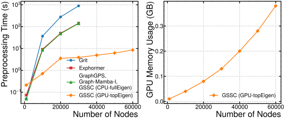
Figure 3: Preprocessing costs per graph.

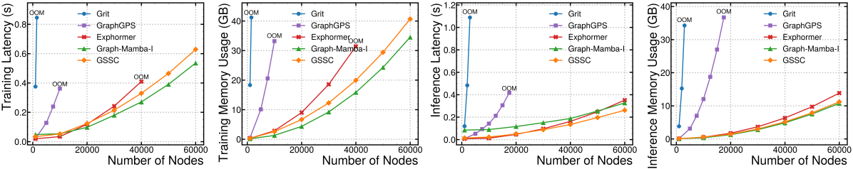
Figure 4: Model training and inference costs per graph.

Preprocessing Costs. As all baseline methods implement preprocessing on CPUs, we first focus on CPU time usage to assess scalability, as illustrated in Fig. 3 (left). Grit notably requires more time due to its repeated multiplications between pairs of $n\times n$ matrices for computing RRWP [70]. Other methods, i.e., Exphormer, GraphGPS, Graph-Mamba-I, and GSSC, may use Laplacian eigendecomposition for graph positional encoding. For these, we follow the implementation of baselines and perform full eigendecomposition on CPUs (limited to 16 cores), depicted by the green and red lines in the figure. Exphormer additionally constructs expander graphs, slightly increasing its preprocessing time. Clearly, full eigendecomposition is costly for large graphs; however, GSSC requires only the smallest $d$ eigenvalues and their eigenvectors. Thus, for large graphs, we can bypass full eigendecomposition and leverage iterative methods on GPUs, such as $\operatorname{torch.lobpcg}$ [58], to obtain the top-$d$ results, which is both fast and GPU memory-efficient (linear in $n$), shown by the orange lines (GPU-topEigen) in the figures with $d=32$. Nonetheless, for small graphs, full eigendecomposition on CPUs remains efficient, aligning with practices in prior studies.

Model Training/Inference Costs. Excluding preprocessing, Fig. 4 benchmarks model training (forward + backward passes) and inference (forward pass only) costs in an inductive node classification setting. All methods are ensured to have the same number of layers and roughly 500k parameters. Methods marked "OOM" indicate out-of-memory errors on a GPU with 48 GB memory when the number of nodes further increases by 5k. GSSC and Graph-Mamba-I emerge as the two most efficient methods. Although Graph-Mamba-I shows slightly better performance during training, this advantage can be attributed to its direct integration with the highly optimized Mamba API [37], and GSSC’s efficiency may also be further improved with hardware-aware optimization in the low-level implementation.

Table 4: Computational costs of GSSC on real-world datasets.

	ZINC-12k	PascalVOC-SP
Avg. # nodes	23.2	479.4
# graphs	12,000	11,355
# epochs	2,000	300
Training time per epoch	$10.9$s	$13.9$s
Total training time	$6.1$h	$1.2$h
Total preprocessing time	$20.6$s	$334.8$s
$\frac{\text{Total preprocessing time}}{\text{Total training time}}$	$0.1\%$	$7.6\%$

Computational Costs of GSSC on Real-World Datasets. The above benchmark evaluates graph (linear) transformers on very large graphs to thoroughly test their scalability. However, as in practice graph transformers are generally applied to smaller graphs [87], where capturing global dependencies can be more beneficial, here we also report the computational costs for two representative and widely used real-world benchmark datasets. The results are presented in Table 4, where ZINC-12k and PascalVOC-SP are included as examples of real-world datasets with the smallest and largest graph sizes, respectively, for evaluating graph transformers. Preprocessing is done on CPUs per graph following previous works due to the relatively small graph sizes, and the number of training epochs used is also the same as prior studies [87, 70, 90]. We can see that the total preprocessing time is negligible for datasets with small graphs (e.g., ZINC-12k), comparable to the duration of a single training epoch (typically the number of training epochs is larger than $100$, meaning a ratio $<1\%$). For datasets with larger graphs (e.g., PascalVOC-SP), preprocessing remains reasonably efficient, consuming less than $10\%$ of the total training time. Notably, the preprocessing time could be further reduced by computing eigendecomposition on GPUs with batched graphs.

6 Conclusion and Limitations

In this work, we study the extension of State Space Models (SSMs) to graphs. We propose Graph State Space Convolution (GSSC) that leverages global permutation-equivariant aggregation and factorizable graph kernels depending on relative graph distances. These operations naturally inherit the advantages of SSMs on sequential data: (1) efficient computation; (2) capability of capturing long-range dependencies; (3) good generalization for various sequence lengths (graph sizes). Numerical experiments demonstrate the superior performance and efficiency of GSSC.

One potential limitation of our work is that precisely computing full eigenvectors could be expensive for large graphs. We discuss possible ways to alleviate the computation overhead in Section 4.2, and our empirical evaluation in Sec. 5.3 shows good scalability even for large graphs with 60k nodes.

7 Acknowledgement

The work is supported by NSF awards PHY-2117997, IIS-2239565, CCF-2402816, and JPMC faculty award 2023. The authors also would like to greatly thank Mufei Li, Haoyu Wang, Xiyuan Wang, and Peihao Wang. Mufei Li introduced the idea of SSM to the team. Xiyuan Wang shared a lot of insights in viewing graphs as point sets. The discussion with Peihao Wang raises the observations on how SSM essentially achieves its three advantages, which inspire the study in this work.

Appendix A Proof of Theorem 4.1

Theorem 4.1 (Counting paths and cycles).

Graph state space convolution Eq. (4) can at least count number of $3$-paths and $3$-cycles. With selection mechanism Eq. (6), it can at least count number of $4$-paths and $4$-cycles. Here “counting” means the node representations can express the number of paths starting at the node or number of cycles involving the node.

Proof.

The number of cycles and paths can be expressed in terms of polynomials of adjacency matrix $\bm{A}$, as shown in [84]. Specifically, let $[P_{m}]_{u,v}$ be number of length-$m$ paths starting at node $u$ and ending at node $v$, and $[C_{m}]_{u}$ be number of length-$m$ cycles involving node $u$, then

$$P_{2} =\bm{A}^{2},$$ (7)

$$C_{3} =\text{diag}(\bm{A}^{3}),$$ (8)

$$P_{3} =\bm{A}^{3}+\bm{A}-\bm{A}\text{diag}(\bm{A^{2}})-\text{diag}(\bm{A}^{2})\bm{A},$$ (9)

$$C_{4} =\text{diag}(\bm{A}^{4})+\text{diag}(\bm{A}^{2})-\text{diag}(\bm{A}^{2}\text{diag}(\bm{A^{2}}))-\text{diag}(\bm{A}\text{diag}(\bm{A}^{2})\bm{A}),$$ (10)

$$P_{4} =\bm{A}^{4}+\bm{A}^{2}+3\bm{A}\odot\bm{A}^{2}-\text{diag}(\bm{A}^{3})\bm{A}-\text{diag}(\bm{A}^{2})\bm{A}^{2}-\bm{A}\text{diag}(\bm{A}^{3})-\bm{A}^{2}\text{diag}(\bm{A}^{2})$$

$$\quad-\bm{A}\text{diag}(\bm{A}^{2})\bm{A}$$ (11)

Here $\text{diag}(\cdot)$ means taking the diagonal of the matrix.

2-paths and 3-cycles. It is clear that GSSC Eq.(4) can compute number of length-2 paths starting at node $u$, using $\sum_{v}[P_{2}]_{u,v}=\sum_{v}[\bm{A}^{2}]_{u,v}=\sum_{v}\langle\bm{\Lambda}\odot p_{u},\bm{\Lambda}\odot p_{v}\rangle$. On other hand, number of $3$-cycles $[C_{3}]_{u}=[\bm{A}^{3}]_{u,u}=\langle\bm{\Lambda}^{3/2}\odot p_{u},\bm{\Lambda}^{3/2}p_{u}\rangle$ can also be implemented by Eq.(4) by setting $\bm{W}_{s}=1$ and $\bm{W}_{o}=0$.

3-paths. $\bm{A}^{3}$ and $\bm{A}$ can be expressed by the similar argument above. Note that $\sum_{v}[\bm{A}\text{diag}(\bm{A}^{2})]_{u,v}=\sum_{v}\bm{A}_{u,v}[\bm{A}^{2}]_{v,v}$. The term $[\bm{A}^{2}]_{v,v}$ can be represented by the node feature after one layer of GSSC, as argued in counting $[C_{3}]_{u}$. Therefore $\sum_{v}\bm{A}_{u,v}[\bm{A}^{2}]_{v,v}=\sum_{v}\langle\bm{\Lambda}^{1/2}\odot p_{u},\bm{\Lambda}^{1/2}p_{v}\rangle[A^{2}]_{v,v}$ can be expressed by a two-layer GSSC. Finally, the term $\sum_{v}[\text{diag}(\bm{A}^{2})\bm{A}]_{u,v}=[\bm{A}^{2}]_{u,u}\cdot\sum_{v}\langle\bm{\Lambda}^{1/2}\odot p_{u},\bm{\Lambda}^{1/2}\odot p_{v}\rangle$ can be computed a one-layer GSSC, by first computing $[\bm{A}^{2}]_{u,u}$ and $\sum_{v}\langle\bm{\Lambda}^{1/2}\odot p_{u},\bm{\Lambda}^{1/2}\odot p_{v}\rangle$ separately and use a intermediate nonlinear MLPs to multiply them.

4-cycles. The term $[\text{diag}(\bm{A}^{4})]_{u}=\bm{A}^{4}_{u,u}=\langle\bm{\Lambda}^{2}p_{u},\bm{\Lambda}^{2}p_{u}\rangle$ can be implemented by one-layer GSSC by letting $\bm{W}_{s}=1,\bm{W}_{o}=0$. Same for $[\text{diag}(\bm{A}^{2})]_{u}$. The term $[\text{diag}(\bm{A}^{2}\text{diag}(\bm{A^{2}}))]_{u}=[\bm{A}^{2}]_{u,u}[\bm{A}^{2}]_{u,u}$ can be implemented by one-layer GSSC with a multiplication nonlinear operation. Finally, note that the last term

$$[\text{diag}(\bm{A}\text{diag}(\bm{A}^{2})\bm{A})]_{u}=\sum_{v}\bm{A}_{u,v}\bm{A}^{2}_{v,v}\bm{A}_{v,u}=\sum_{v}\bm{A}_{u,v}\bm{A}_{u,v}\bm{A}^{2}_{v,v}.$$ (12)

We know that $x_{v}:=\bm{A}^{2}_{v,v}$ can be encoded into node feature after one-layer GSSC. Now the whole term $\sum_{v}\bm{A}_{u,v}\bm{A}_{u,v}x_{v}$ can be transformed into

$$\begin{split}\sum_{v}\bm{A}_{u,v}\bm{A}_{u,v}x_{v}&=\sum_{v}\langle\bm{\Lambda}^{1/2}p_{u},\bm{\Lambda}^{1/2}p_{v}\rangle\langle\bm{\Lambda}^{1/2}p_{u},\bm{\Lambda}^{1/2}p_{v}\rangle x_{v}\\ &=\langle\bm{\Lambda}^{1/2}p_{u}\sum_{v},\langle\bm{\Lambda}^{1/2}p_{u},\bm{\Lambda}^{1/2}p_{v}\rangle p_{v}\odot x_{v}\rangle=\langle\bm{\Lambda}^{1/2}p_{u},\tilde{z}_{u}\rangle,\end{split}$$ (13)

where $\tilde{z}_{u}$ is a node-feature-dependent PE, which can be implemented by Eq.(6). The readout $\langle\bm{\Lambda}^{1/2}p_{u},\tilde{z}_{u}\rangle$, again, can be implemented by letting $\bm{W}_{o}=0$ and $\bm{W}_{s}=1$.

4-paths. All terms can be expressed by the same argument in counting 3-paths, except $\bm{A}\odot\bm{A}^{2}$ and $\bm{A}\text{diag}(\bm{A}^{2})\bm{A}$. To compute $\sum_{v}[\bm{A}\odot\bm{A}^{2}]_{u,v}=\sum_{v}\bm{A}_{u,v}\bm{A}^{2}_{u,v}$, note that this follows the same argument as in Eq.(13), with $x_{v}$ replaced by $1$ and the second $\bm{A}_{u,v}$ replaced by $\bm{A}^{2}_{u,v}$. To compute $\sum_{v}[\bm{A}\text{diag}(\bm{A}^{2})\bm{A}]_{u,v}$, note that

$$\sum_{v}[\bm{A}\text{diag}(\bm{A}^{2})\bm{A}]_{u,v}=\sum_{w}\bm{A}_{u,w}\bm{A}^{2}_{w,w}\sum_{v}\bm{A}_{w,v}.$$ (14)

Therefore, we can first use one-layer GSSC to encode $\bm{A}_{w,w}^{2}$ and $\sum_{v}\bm{A}_{w,v}$ into node features, multiply them together to get $x_{w}=\bm{A}_{w,w}^{2}\cdot\sum_{v}\bm{A}_{w,v}$, and then apply another GSSC layer with kernel $\bm{A}_{u,w}$ to get desired output $\sum_{w}\bm{A}_{u,w}x_{w}$. ∎

Appendix B Experimental Details

B.1 Datasets Description

Table 5: Dataset statistics used in the experiments.

Dataset	# Graphs	Avg. # nodes	Avg. # edges	Prediction level	Prediction task
Cycle-counting	5,000	18.8	31.3	node	regression
ZINC-subset	12,000	23.2	24.9	graph	regression
ZINC-full	249,456	23.1	24.9	graph	regression
ogbg-molhiv	41,127	25.5	27.5	graph	binary classif.
MNIST	70,000	70.6	564.5	graph	10-class classif.
CIFAR10	60,000	117.6	941.1	graph	10-class classif.
PATTERN	14,000	118.9	3,039.3	node	binary classifi.
CLUSTER	12,000	117.2	2,150.9	node	6-class classif.
Peptides-func	15,535	150.9	307.3	graph	10-class classif.
Peptides-struct	15,535	150.9	307.3	graph	regression
PascalVOC-SP	11,355	479.4	2,710.5	node	21-class classif.

Graph Substructure Counting [13, 123, 48] is a synthetic dataset containing 5k graphs generated from different distributions (Erdős-Rényi random graphs, random regular graphs, etc. see [13] Appendix M.2.1). Each node is labeled by the number of $3,4,5,6$-cycles that involves the node. The task is to predict the number of cycles as node-level regression. The training/validation/test set is randomly split by 3:2:5.

ZINC [25] (MIT License) has two versions of datasets with different splits. ZINC-subset contains 12k molecular graphs from the ZINC database of commercially available chemical compounds. These represent small molecules with the number of atoms between 9 and 37. Each node represents a heavy atom (28 atom types) and each edge represents a chemical bond (3 types). The task is to do graph-level regression on the constrained solubility (logP) of the molecule. The dataset comes with a predefined 10K/1K/1K train/validation/test split. ZINC-full is similar to ZINC-subset but with 250k molecular graphs instead.

ogbg-molhiv [46] (MIT License) are molecular property prediction datasets adopted by OGB from MoleculeNet [113]. These datasets use a common node (atom) and edge (bond) featurization that represent chemophysical properties. The task is a binary graph-level classification of the molecule’s fitness to inhibit HIV replication. The dataset split is predefined as in [46].

MNIST and CIFAR10 [25] (CC BY-SA 3.0 and MIT License) are derived from image classification datasets, where each image graph is constructed by the 8 nearest-neighbor graph of SLIC superpixels for each image. The task is a 10-class graph-level classification and standard dataset splits follow the original image classification datasets, i.e., for MNIST 55K/5K/10K and for CIFAR10 45K/5K/10K train/validation/test graphs.

PATTERN and CLUSTER [25] (MIT License) are synthetic datasets of community structures, sampled from the Stochastic Block Model. Both tasks are an inductive node-level classification. PATTERN is to detect nodes in a graph into one of 100 possible sub-graph patterns that are randomly generated with different SBM parameters than the rest of the graph. In CLUSTER, every graph is composed of 6 SBM-generated clusters, and there is a corresponding test node in each cluster containing a unique cluster ID. The task is to predict the cluster ID of these 6 test nodes.

Peptides-func and Peptides-struct [27] (MIT License) are derived from 15k peptides retrieved from SATPdb [91]. Both datasets use the same set of graphs but the prediction tasks are different. Peptides-func is a graph-level classification task with 10 functional labels associated with peptide functions. Peptides-struct is a graph-level regression task to predict 11 structural properties of the molecules.

PascalVOC-SP [27] (MIT License) is a node classification dataset based on the Pascal VOC 2011 image dataset [28]. Superpixel nodes are extracted using the SLIC algorithm [1] and a rag-boundary graph that interconnects these nodes are constructed. The task is to classify the node into corresponding object classes, which is analogous to the semantic segmentation.

B.2 Random Seeds and Dataset Splits

All included datasets have standard training/validation/test splits. We follow previous works reporting the test results according to the best validation performance, and the results of every dataset are evaluated and averaged over five different random seeds [87, 70, 90]. Due to the extremely long running time of ZINC-Full (which requires over 80 hours to train one seed on an Nvidia RTX 6000 Ada since it uses 2k epochs for training following previous works [87, 70]), its results are averaged over three random seeds.

B.3 Hyperparameters

Table 6, 7, 8, and 9 detail the hyperparameters used for experiments in Sec. 5. We generally follow configurations from prior works [87, 90]. Notably, the selective mechanism (i.e., Eq. (6)) is only employed for graph substructure counting tasks, and GSSC utilizes the smallest $d=32$ eigenvalues and their eigenvectors for all datasets except molecular ones, which use $d=16$. Consistent with previous research [87, 70], we also maintain the number of model parameters at around 500k for the ZINC, PATTERN, CLUSTER, and LRGB datasets, and approximately 100k for the MNIST and CIFAR10 datasets.

Since our implementation is based on the framework of GraphGPS [87], which combines the learned node representations from the MPNN and the global module (GSSC in our case) in each layer, dropout is applied for regularization to the outputs from both modules, as indicated by MPNN-dropout and GSSC-dropout in the hyperparameter tables.

Table 6: Model hyperparameters for graph substructure counting datasets.

Hyperparameter	$3$-Cycle	$4$-Cycle	$5$-Cycle
# Layers	4	4	4
Hidden dim	96	96	96
MPNN	GatedGCN	GatedGCN	GatedGCN
Lap dim $d$	16	16	16
Selective	True	True	True
Batch size	256	256	256
Learning Rate	0.001	0.001	0.001
Weight decay	1e-5	1e-5	1e-5
MPNN-dropout	0.3	0.3	0.3
GSSC-dropout	0.3	0.3	0.3
# Parameters	926k	926k	926k

Table 7: Model hyperparameters for molecular property prediction datasets.

Hyperparameter	ZINC-12k	ZINC-Full	ogbg-molhiv
# Layers	10	10	6
Hidden dim	64	64	64
MPNN	GINE	GINE	GatedGCN
Lap dim $d$	16	16	16
Selective	False	False	False
Batch size	32	128	32
Learning Rate	0.001	0.002	0.002
Weight decay	1e-5	0.001	0.001
MPNN-dropout	0	0.1	0.3
GSSC-dropout	0.6	0	0
# Parameters	436k	436k	351k

Table 8: Model hyperparameters for datasets from Long Range Graph Benchmark (LRGB) [27].

Hyperparameter	PascalVOC-SP	Peptides-func	Peptides-struct
# Layers	4	4	4
Hidden dim	96	96	96
MPNN	GatedGCN	GatedGCN	GatedGCN
Lap dim $d$	32	32	32
Selective	False	False	False
Batch size	32	128	128
Learning Rate	0.002	0.003	0.001
Weight decay	0.1	0.1	0.1
MPNN-dropout	0	0.1	0.1
GSSC-dropout	0.5	0.1	0.3
# Parameters	375k	410k	410k

Table 9: Model hyperparameters for datasets from GNN Benchmark [25].

Hyperparameter	MNIST	CIFAR10	PATTERN	CLUSTER
# Layers	3	3	24	24
Hidden dim	52	52	36	36
MPNN	GatedGCN	GatedGCN	GatedGCN	GatedGCN
Lap dim $d$	32	32	32	32
Selective	False	False	False	False
Batch size	16	16	32	16
Learning Rate	0.005	0.005	0.001	0.001
Weight decay	0.01	0.01	0.1	0.1
MPNN-dropout	0.1	0.1	0.1	0.3
GSSC-dropout	0.1	0.1	0.5	0.3
# Parameters	133k	131k	539k	539k

Appendix C Supplementary Experiments

In this section, we present supplementary experiments comparing GSSC with previous graph mamba works, i.e., Graph-Mamba-I [103] and Graph-Mamba-II [5]. As shown in Table 10, GSSC significantly outperforms both models on all datasets. We attempted to evaluate these works on additional datasets included in our experiments, such as ZINC-12k, but encountered challenges. Specifically, Graph-Mamba-II has only an empty GitHub repository available, and Graph-Mamba-I raises persistent NaN (Not a Number) errors when evaluated on other datasets. Our investigation suggests that these errors of Graph-Mamba-I stem from fundamental issues in their architecture and implementation, and there is no easy way to fix them, i.e., they are not caused by any easy-to-find risky operations such as $\log(\text{small negative numbers})$ or $\frac{1}{0}$. Consequently, Graph-Mamba-I (and Graph-Mamba-II) may potentially exhibit severe numerical instability and cannot be applied to some datasets. Prior to encountering the NaN error, the best observed MAE for Graph-Mamba-I on ZINC-12k was $\sim 0.10$.

Table 10: Comparing with previous graph mamba works. $\textbf{Bold}^{\dagger}$ denotes the best results. Results are reported as $\text{mean}_{\pm\text{std}}$.

	ZINC-12k	MNIST	CIFAR10	PATTERN	CLUSTER	PascalVOC-SP	Peptides-func	Peptides-struct
	MAE $\downarrow$	Accuracy $\uparrow$	Accuracy $\uparrow$	Accuracy $\uparrow$	Accuracy $\uparrow$	F1 score$\uparrow$	AP $\uparrow$	MAE $\downarrow$
Graph-Mamba-I	NaN	${98.420}_{\pm 0.080}$	$73.700_{\pm 0.340}$	$86.710_{\pm 0.050}$	$76.800_{\pm 0.360}$	${0.4191}_{\pm 0.0126}$	${0.6739}_{\pm 0.0087}$	${0.2478}_{\pm 0.0016}$
Graph-Mamba-II	N/A	$98.390_{\pm 0.180}$	$75.760_{\pm 0.420}$	$87.140_{\pm 0.120}$	N/A	$0.4393_{\pm 0.0112}$	$0.7071_{\pm 0.0083}$	$0.2473_{\pm 0.0025}$
GSSC	$\mathbf{0.064}^{\dagger}_{\pm 0.002}$	$\mathbf{98.492}^{\dagger}_{\pm 0.051}$	$\mathbf{77.642}^{\dagger}_{\pm 0.456}$	$\mathbf{87.510}^{\dagger}_{\pm 0.082}$	$\mathbf{79.156}^{\dagger}_{\pm 0.152}$	$\mathbf{0.4561}^{\dagger}_{\pm 0.0039}$	$\mathbf{0.7081}^{\dagger}_{\pm 0.0062}$	$\mathbf{0.2459}^{\dagger}_{\pm 0.0020}$

References

- [1] Radhakrishna Achanta, Appu Shaji, Kevin Smith, Aurelien Lucchi, Pascal Fua, and Sabine Süsstrunk. Slic superpixels compared to state-of-the-art superpixel methods. IEEE transactions on pattern analysis and machine intelligence, 34(11):2274–2282, 2012.
- [2] Uri Alon and Eran Yahav. On the bottleneck of graph neural networks and its practical implications. In International Conference on Learning Representations, 2021.
- [3] Dominique Beaini, Saro Passaro, Vincent Létourneau, Will Hamilton, Gabriele Corso, and Pietro Liò. Directional graph networks. In International Conference on Machine Learning, pages 748–758. PMLR, 2021.
- [4] Ali Behrouz and Farnoosh Hashemi. Graph mamba: Towards learning on graphs with state space models. arXiv preprint arXiv:2402.08678, 2024.
- [5] Ali Behrouz and Farnoosh Hashemi. Graph mamba: Towards learning on graphs with state space models. ArXiv, abs/2402.08678, 2024.
- [6] Mikhail Belkin and Partha Niyogi. Laplacian eigenmaps for dimensionality reduction and data representation. Neural computation, 15(6):1373–1396, 2003.
- [7] Deyu Bo, Chuan Shi, Lele Wang, and Renjie Liao. Specformer: Spectral graph neural networks meet transformers. In The Eleventh International Conference on Learning Representations, 2022.
- [8] Xavier Bresson and Thomas Laurent. Residual gated graph convnets. arXiv preprint arXiv:1711.07553, 2017.
- [9] Deli Chen, Yankai Lin, Wei Li, Peng Li, Jie Zhou, and Xu Sun. Measuring and relieving the over-smoothing problem for graph neural networks from the topological view. In Proceedings of the AAAI conference on artificial intelligence, volume 34, pages 3438–3445, 2020.
- [10] Dexiong Chen, Leslie O’Bray, and Karsten Borgwardt. Structure-aware transformer for graph representation learning. In Kamalika Chaudhuri, Stefanie Jegelka, Le Song, Csaba Szepesvari, Gang Niu, and Sivan Sabato, editors, Proceedings of the 39th International Conference on Machine Learning, volume 162 of Proceedings of Machine Learning Research, pages 3469–3489. PMLR, 17–23 Jul 2022.
- [11] Dexiong Chen, Leslie O’Bray, and Karsten Borgwardt. Structure-aware transformer for graph representation learning. In International Conference on Machine Learning, pages 3469–3489. PMLR, 2022.
- [12] Jinsong Chen, Kaiyuan Gao, Gaichao Li, and Kun He. Nagphormer: A tokenized graph transformer for node classification in large graphs. In The Eleventh International Conference on Learning Representations, 2022.
- [13] Zhengdao Chen, Lei Chen, Soledad Villar, and Joan Bruna. Can graph neural networks count substructures? Advances in neural information processing systems, 33:10383–10395, 2020.
- [14] Eli Chien, Jianhao Peng, Pan Li, and Olgica Milenkovic. Adaptive universal generalized pagerank graph neural network. In International Conference on Learning Representations, 2021.
- [15] Rewon Child, Scott Gray, Alec Radford, and Ilya Sutskever. Generating long sequences with sparse transformers. ArXiv, abs/1904.10509, 2019.
- [16] Krzysztof Choromanski, Valerii Likhosherstov, David Dohan, Xingyou Song, Andreea Gane, Tamas Sarlos, Peter Hawkins, Jared Davis, Afroz Mohiuddin, Lukasz Kaiser, et al. Rethinking attention with performers. arXiv preprint arXiv:2009.14794, 2020.
- [17] Krzysztof Marcin Choromanski. Taming graph kernels with random features. In International Conference on Machine Learning, pages 5964–5977. PMLR, 2023.
- [18] Fan Chung. The heat kernel as the pagerank of a graph. Proceedings of the National Academy of Sciences, 104(50):19735–19740, 2007.
- [19] Gabriele Corso, Luca Cavalleri, Dominique Beaini, Pietro Liò, and Petar Veličković. Principal neighbourhood aggregation for graph nets. Advances in Neural Information Processing Systems, 33:13260–13271, 2020.
- [20] Giannis Daras, Nikita Kitaev, Augustus Odena, and Alexandros G Dimakis. Smyrf-efficient attention using asymmetric clustering. Advances in Neural Information Processing Systems, 33:6476–6489, 2020.
- [21] Francesco Di Giovanni, Lorenzo Giusti, Federico Barbero, Giulia Luise, Pietro Lio, and Michael M Bronstein. On over-squashing in message passing neural networks: The impact of width, depth, and topology. In International Conference on Machine Learning, pages 7865–7885. PMLR, 2023.
- [22] James Durbin and Siem Jan Koopman. Time series analysis by state space methods, volume 38. OUP Oxford, 2012.
- [23] David K Duvenaud, Dougal Maclaurin, Jorge Iparraguirre, Rafael Bombarell, Timothy Hirzel, Alán Aspuru-Guzik, and Ryan P Adams. Convolutional networks on graphs for learning molecular fingerprints. Advances in neural information processing systems, 28, 2015.
- [24] Vijay Prakash Dwivedi and Xavier Bresson. A generalization of transformer networks to graphs. ArXiv, abs/2012.09699, 2020.
- [25] Vijay Prakash Dwivedi, Chaitanya K Joshi, Anh Tuan Luu, Thomas Laurent, Yoshua Bengio, and Xavier Bresson. Benchmarking graph neural networks. Journal of Machine Learning Research, 24(43):1–48, 2023.
- [26] Vijay Prakash Dwivedi, Anh Tuan Luu, Thomas Laurent, Yoshua Bengio, and Xavier Bresson. Graph neural networks with learnable structural and positional representations. In International Conference on Learning Representations, 2021.
- [27] Vijay Prakash Dwivedi, Ladislav Rampášek, Michael Galkin, Ali Parviz, Guy Wolf, Anh Tuan Luu, and Dominique Beaini. Long range graph benchmark. Advances in Neural Information Processing Systems, 35:22326–22340, 2022.
- [28] Mark Everingham, Luc Van Gool, Christopher KI Williams, John Winn, and Andrew Zisserman. The pascal visual object classes (voc) challenge. International journal of computer vision, 88:303–338, 2010.
- [29] Wenqi Fan, Yao Ma, Qing Li, Yuan He, Eric Zhao, Jiliang Tang, and Dawei Yin. Graph neural networks for social recommendation. In The world wide web conference, pages 417–426, 2019.
- [30] Fabrizio Frasca, Beatrice Bevilacqua, Michael Bronstein, and Haggai Maron. Understanding and extending subgraph gnns by rethinking their symmetries. Advances in Neural Information Processing Systems, 35:31376–31390, 2022.
- [31] Daniel Y Fu, Tri Dao, Khaled Kamal Saab, Armin W Thomas, Atri Rudra, and Christopher Re. Hungry hungry hippos: Towards language modeling with state space models. In The Eleventh International Conference on Learning Representations, 2022.
- [32] Daniel Y Fu, Elliot L Epstein, Eric Nguyen, Armin W Thomas, Michael Zhang, Tri Dao, Atri Rudra, and Christopher Ré. Simple hardware-efficient long convolutions for sequence modeling. In International Conference on Machine Learning, pages 10373–10391. PMLR, 2023.
- [33] Victor Fung, Jiaxin Zhang, Eric Juarez, and Bobby G Sumpter. Benchmarking graph neural networks for materials chemistry. npj Computational Materials, 7(1):84, 2021.
- [34] C Lee Giles and Tom Maxwell. Learning, invariance, and generalization in high-order neural networks. Applied optics, 26(23):4972–4978, 1987.
- [35] David F Gleich. Pagerank beyond the web. siam REVIEW, 57(3):321–363, 2015.
- [36] Alex Graves. Generating sequences with recurrent neural networks. arXiv preprint arXiv:1308.0850, 2013.
- [37] Albert Gu and Tri Dao. Mamba: Linear-time sequence modeling with selective state spaces. arXiv preprint arXiv:2312.00752, 2023.
- [38] Albert Gu, Tri Dao, Stefano Ermon, Atri Rudra, and Christopher Ré. Hippo: Recurrent memory with optimal polynomial projections. Advances in neural information processing systems, 33:1474–1487, 2020.
- [39] Albert Gu, Karan Goel, Ankit Gupta, and Christopher Ré. On the parameterization and initialization of diagonal state space models. Advances in Neural Information Processing Systems, 35:35971–35983, 2022.
- [40] Albert Gu, Karan Goel, and Christopher Re. Efficiently modeling long sequences with structured state spaces. In International Conference on Learning Representations, 2021.
- [41] Albert Gu, Isys Johnson, Karan Goel, Khaled Saab, Tri Dao, Atri Rudra, and Christopher Ré. Combining recurrent, convolutional, and continuous-time models with linear state space layers. Advances in neural information processing systems, 34:572–585, 2021.
- [42] Zhiwei Guo and Heng Wang. A deep graph neural network-based mechanism for social recommendations. IEEE Transactions on Industrial Informatics, 17(4):2776–2783, 2020.
- [43] Ankit Gupta, Albert Gu, and Jonathan Berant. Diagonal state spaces are as effective as structured state spaces. In S. Koyejo, S. Mohamed, A. Agarwal, D. Belgrave, K. Cho, and A. Oh, editors, Advances in Neural Information Processing Systems, volume 35, pages 22982–22994. Curran Associates, Inc., 2022.
- [44] Insu Han, Rajesh Jayaram, Amin Karbasi, Vahab Mirrokni, David Woodruff, and Amir Zandieh. Hyperattention: Long-context attention in near-linear time. In The Twelfth International Conference on Learning Representations, 2023.
- [45] Ramin Hasani, Mathias Lechner, Tsun-Hsuan Wang, Makram Chahine, Alexander Amini, and Daniela Rus. Liquid structural state-space models. In The Eleventh International Conference on Learning Representations, 2022.
- [46] Weihua Hu, Matthias Fey, Marinka Zitnik, Yuxiao Dong, Hongyu Ren, Bowen Liu, Michele Catasta, and Jure Leskovec. Open graph benchmark: Datasets for machine learning on graphs. Advances in neural information processing systems, 33:22118–22133, 2020.
- [47] Yinan Huang, William Lu, Joshua Robinson, Yu Yang, Muhan Zhang, Stefanie Jegelka, and Pan Li. On the stability of expressive positional encodings for graph neural networks. In The Twelfth International Conference on Learning Representations, 2024.
- [48] Yinan Huang, Xingang Peng, Jianzhu Ma, and Muhan Zhang. Boosting the cycle counting power of graph neural networks with i2-gnns. In The Eleventh International Conference on Learning Representations, 2022.
- [49] Rob Hyndman, Anne B Koehler, J Keith Ord, and Ralph D Snyder. Forecasting with exponential smoothing: the state space approach. Springer Science & Business Media, 2008.
- [50] Piotr Indyk and Rajeev Motwani. Approximate nearest neighbors: towards removing the curse of dimensionality. In Proceedings of the thirtieth annual ACM symposium on Theory of computing, pages 604–613, 1998.
- [51] Rudolph Emil Kalman. A new approach to linear filtering and prediction problems. 1960.
- [52] Angelos Katharopoulos, Apoorv Vyas, Nikolaos Pappas, and François Fleuret. Transformers are RNNs: Fast autoregressive transformers with linear attention. In Hal Daumé III and Aarti Singh, editors, Proceedings of the 37th International Conference on Machine Learning, volume 119 of Proceedings of Machine Learning Research, pages 5156–5165. PMLR, 13–18 Jul 2020.
- [53] Amirhossein Kazemnejad, Inkit Padhi, Karthikeyan Natesan Ramamurthy, Payel Das, and Siva Reddy. The impact of positional encoding on length generalization in transformers. Advances in Neural Information Processing Systems, 36, 2024.
- [54] Nicolas Keriven. Not too little, not too much: a theoretical analysis of graph (over) smoothing. Advances in Neural Information Processing Systems, 35:2268–2281, 2022.
- [55] Jinwoo Kim, Dat Nguyen, Seonwoo Min, Sungjun Cho, Moontae Lee, Honglak Lee, and Seunghoon Hong. Pure transformers are powerful graph learners. Advances in Neural Information Processing Systems, 35:14582–14595, 2022.
- [56] Thomas N Kipf and Max Welling. Semi-supervised classification with graph convolutional networks. In International Conference on Learning Representations, 2016.
- [57] Nikita Kitaev, Łukasz Kaiser, and Anselm Levskaya. Reformer: The efficient transformer. arXiv preprint arXiv:2001.04451, 2020.
- [58] Andrew V Knyazev. Toward the optimal preconditioned eigensolver: Locally optimal block preconditioned conjugate gradient method. SIAM journal on scientific computing, 23(2):517–541, 2001.
- [59] Kezhi Kong, Jiuhai Chen, John Kirchenbauer, Renkun Ni, C Bayan Bruss, and Tom Goldstein. Goat: A global transformer on large-scale graphs. In International Conference on Machine Learning, pages 17375–17390. PMLR, 2023.
- [60] Devin Kreuzer, Dominique Beaini, Will Hamilton, Vincent Létourneau, and Prudencio Tossou. Rethinking graph transformers with spectral attention. Advances in Neural Information Processing Systems, 34:21618–21629, 2021.
- [61] Alex Krizhevsky, Ilya Sutskever, and Geoffrey E Hinton. Imagenet classification with deep convolutional neural networks. Advances in neural information processing systems, 25, 2012.
- [62] Alex Krizhevsky, Ilya Sutskever, and Geoffrey E Hinton. Imagenet classification with deep convolutional neural networks. Communications of the ACM, 60(6):84–90, 2017.
- [63] Cornelius Lanczos. An iteration method for the solution of the eigenvalue problem of linear differential and integral operators. 1950.
- [64] Yann LeCun, Léon Bottou, Yoshua Bengio, and Patrick Haffner. Gradient-based learning applied to document recognition. Proceedings of the IEEE, 86(11):2278–2324, 1998.
- [65] Pan Li, I Chien, and Olgica Milenkovic. Optimizing generalized pagerank methods for seed-expansion community detection. Advances in Neural Information Processing Systems, 32, 2019.
- [66] Pan Li, Yanbang Wang, Hongwei Wang, and Jure Leskovec. Distance encoding: Design provably more powerful neural networks for graph representation learning. Advances in Neural Information Processing Systems, 33:4465–4478, 2020.
- [67] Yuhong Li, Tianle Cai, Yi Zhang, Deming Chen, and Debadeepta Dey. What makes convolutional models great on long sequence modeling? In The Eleventh International Conference on Learning Representations, 2023.
- [68] Derek Lim, Joshua David Robinson, Lingxiao Zhao, Tess Smidt, Suvrit Sra, Haggai Maron, and Stefanie Jegelka. Sign and basis invariant networks for spectral graph representation learning. In The Eleventh International Conference on Learning Representations, 2022.
- [69] Yaron Lipman, Raif M Rustamov, and Thomas A Funkhouser. Biharmonic distance. ACM Transactions on Graphics (TOG), 29(3):1–11, 2010.
- [70] Liheng Ma, Chen Lin, Derek Lim, Adriana Romero-Soriano, Puneet K Dokania, Mark Coates, Philip Torr, and Ser-Nam Lim. Graph inductive biases in transformers without message passing. In International Conference on Machine Learning, pages 23321–23337. PMLR, 2023.
- [71] Xuezhe Ma, Chunting Zhou, Xiang Kong, Junxian He, Liangke Gui, Graham Neubig, Jonathan May, and Luke Zettlemoyer. Mega: Moving average equipped gated attention. In The Eleventh International Conference on Learning Representations, 2022.
- [72] Sohir Maskey, Ali Parviz, Maximilian Thiessen, Hannes Stärk, Ylli Sadikaj, and Haggai Maron. Generalized laplacian positional encoding for graph representation learning. In NeurIPS 2022 Workshop on Symmetry and Geometry in Neural Representations, 2022.
- [73] Harsh Mehta, Ankit Gupta, Ashok Cutkosky, and Behnam Neyshabur. Long range language modeling via gated state spaces. In The Eleventh International Conference on Learning Representations, 2022.
- [74] Grégoire Mialon, Dexiong Chen, Margot Selosse, and Julien Mairal. Graphit: Encoding graph structure in transformers. arXiv preprint arXiv:2106.05667, 2021.
- [75] Siqi Miao, Zhiyuan Lu, Mia Liu, Javier Duarte, and Pan Li. Locality-sensitive hashing-based efficient point transformer with applications in high-energy physics. International Conference on Machine Learning, 2024.
- [76] Christopher Morris, Martin Ritzert, Matthias Fey, William L Hamilton, Jan Eric Lenssen, Gaurav Rattan, and Martin Grohe. Weisfeiler and leman go neural: Higher-order graph neural networks. In Proceedings of the AAAI conference on artificial intelligence, volume 33, pages 4602–4609, 2019.
- [77] Khang Nguyen, Nong Minh Hieu, Vinh Duc Nguyen, Nhat Ho, Stanley Osher, and Tan Minh Nguyen. Revisiting over-smoothing and over-squashing using ollivier-ricci curvature. In International Conference on Machine Learning, pages 25956–25979. PMLR, 2023.
- [78] Giannis Nikolentzos and Michalis Vazirgiannis. Random walk graph neural networks. Advances in Neural Information Processing Systems, 33:16211–16222, 2020.
- [79] Lawrence Page, Sergey Brin, Rajeev Motwani, Terry Winograd, et al. The pagerank citation ranking: Bringing order to the web. 1999.
- [80] Christopher C Paige. Computational variants of the lanczos method for the eigenproblem. IMA Journal of Applied Mathematics, 10(3):373–381, 1972.
- [81] José Luis Palacios. Resistance distance in graphs and random walks. International Journal of Quantum Chemistry, 81(1):29–33, 2001.
- [82] Razvan Pascanu, Tomas Mikolov, and Yoshua Bengio. On the difficulty of training recurrent neural networks. In International conference on machine learning, pages 1310–1318. Pmlr, 2013.
- [83] Bo Peng, Eric Alcaide, Quentin Gregory Anthony, Alon Albalak, Samuel Arcadinho, Stella Biderman, Huanqi Cao, Xin Cheng, Michael Nguyen Chung, Leon Derczynski, Xingjian Du, Matteo Grella, Kranthi Kiran GV, Xuzheng He, Haowen Hou, Przemyslaw Kazienko, Jan Kocon, Jiaming Kong, Bartłomiej Koptyra, Hayden Lau, Jiaju Lin, Krishna Sri Ipsit Mantri, Ferdinand Mom, Atsushi Saito, Guangyu Song, Xiangru Tang, Johan S. Wind, Stanisław Woźniak, Zhenyuan Zhang, Qinghua Zhou, Jian Zhu, and Rui-Jie Zhu. RWKV: Reinventing RNNs for the transformer era. In The 2023 Conference on Empirical Methods in Natural Language Processing, 2023.
- [84] SN Perepechko and AN Voropaev. The number of fixed length cycles in an undirected graph. explicit formulae in case of small lengths. Mathematical Modeling and Computational Physics (MMCP2009), 148, 2009.
- [85] Michael Poli, Stefano Massaroli, Eric Nguyen, Daniel Y Fu, Tri Dao, Stephen Baccus, Yoshua Bengio, Stefano Ermon, and Christopher Re. Hyena hierarchy: Towards larger convolutional language models. In Andreas Krause, Emma Brunskill, Kyunghyun Cho, Barbara Engelhardt, Sivan Sabato, and Jonathan Scarlett, editors, Proceedings of the 40th International Conference on Machine Learning, volume 202 of Proceedings of Machine Learning Research, pages 28043–28078. PMLR, 23–29 Jul 2023.
- [86] Zhen Qin, Xiaodong Han, Weixuan Sun, Bowen He, Dong Li, Dongxu Li, Yuchao Dai, Lingpeng Kong, and Yiran Zhong. Toeplitz neural network for sequence modeling. In The Eleventh International Conference on Learning Representations, 2022.
- [87] Ladislav Rampášek, Michael Galkin, Vijay Prakash Dwivedi, Anh Tuan Luu, Guy Wolf, and Dominique Beaini. Recipe for a general, powerful, scalable graph transformer. Advances in Neural Information Processing Systems, 35:14501–14515, 2022.
- [88] Isaac Reid, Adrian Weller, and Krzysztof M Choromanski. Quasi-monte carlo graph random features. Advances in Neural Information Processing Systems, 36, 2024.
- [89] T Konstantin Rusch, Michael M Bronstein, and Siddhartha Mishra. A survey on oversmoothing in graph neural networks. arXiv preprint arXiv:2303.10993, 2023.
- [90] Hamed Shirzad, Ameya Velingker, Balaji Venkatachalam, Danica J Sutherland, and Ali Kemal Sinop. Exphormer: Sparse transformers for graphs. In International Conference on Machine Learning, pages 31613–31632. PMLR, 2023.
- [91] Sandeep Singh, Kumardeep Chaudhary, Sandeep Kumar Dhanda, Sherry Bhalla, Salman Sadullah Usmani, Ankur Gautam, Abhishek Tuknait, Piyush Agrawal, Deepika Mathur, and Gajendra PS Raghava. Satpdb: a database of structurally annotated therapeutic peptides. Nucleic acids research, 44(D1):D1119–D1126, 2016.
- [92] Jimmy TH Smith, Andrew Warrington, and Scott Linderman. Simplified state space layers for sequence modeling. In The Eleventh International Conference on Learning Representations, 2022.
- [93] Alexander J Smola and Risi Kondor. Kernels and regularization on graphs. In Learning Theory and Kernel Machines: 16th Annual Conference on Learning Theory and 7th Kernel Workshop, COLT/Kernel 2003, Washington, DC, USA, August 24-27, 2003. Proceedings, pages 144–158. Springer, 2003.
- [94] Jonathan M Stokes, Kevin Yang, Kyle Swanson, Wengong Jin, Andres Cubillos-Ruiz, Nina M Donghia, Craig R MacNair, Shawn French, Lindsey A Carfrae, Zohar Bloom-Ackermann, et al. A deep learning approach to antibiotic discovery. Cell, 180(4):688–702, 2020.
- [95] Yutao Sun, Li Dong, Shaohan Huang, Shuming Ma, Yuqing Xia, Jilong Xue, Jianyong Wang, and Furu Wei. Retentive network: A successor to transformer for large language models, 2024.
- [96] Ilya Sutskever, Oriol Vinyals, and Quoc V Le. Sequence to sequence learning with neural networks. Advances in neural information processing systems, 27, 2014.
- [97] Yi Tay, Mostafa Dehghani, Samira Abnar, Yikang Shen, Dara Bahri, Philip Pham, Jinfeng Rao, Liu Yang, Sebastian Ruder, and Donald Metzler. Long range arena: A benchmark for efficient transformers. arXiv preprint arXiv:2011.04006, 2020.
- [98] Jake Topping, Francesco Di Giovanni, Benjamin Paul Chamberlain, Xiaowen Dong, and Michael M. Bronstein. Understanding over-squashing and bottlenecks on graphs via curvature. In International Conference on Learning Representations, 2022.
- [99] Arnold Tustin. A method of analysing the behaviour of linear systems in terms of time series. Journal of the Institution of Electrical Engineers-Part IIA: Automatic Regulators and Servo Mechanisms, 94(1):130–142, 1947.
- [100] Ashish Vaswani, Noam Shazeer, Niki Parmar, Jakob Uszkoreit, Llion Jones, Aidan N Gomez, Łukasz Kaiser, and Illia Polosukhin. Attention is all you need. Advances in neural information processing systems, 30, 2017.
- [101] Petar Veličković, Guillem Cucurull, Arantxa Casanova, Adriana Romero, Pietro Liò, and Yoshua Bengio. Graph attention networks. In International Conference on Learning Representations, 2018.
- [102] Ameya Velingker, Ali Sinop, Ira Ktena, Petar Veličković, and Sreenivas Gollapudi. Affinity-aware graph networks. Advances in Neural Information Processing Systems, 36, 2024.
- [103] Chloe Wang, Oleksii Tsepa, Jun Ma, and Bo Wang. Graph-mamba: Towards long-range graph sequence modeling with selective state spaces. arXiv preprint arXiv:2402.00789, 2024.
- [104] Haorui Wang, Haoteng Yin, Muhan Zhang, and Pan Li. Equivariant and stable positional encoding for more powerful graph neural networks. In International Conference on Learning Representations, 2021.
- [105] Jue Wang, Wentao Zhu, Pichao Wang, Xiang Yu, Linda Liu, Mohamed Omar, and Raffay Hamid. Selective structured state-spaces for long-form video understanding. In Proceedings of the IEEE/CVF Conference on Computer Vision and Pattern Recognition, pages 6387–6397, 2023.
- [106] Sinong Wang, Belinda Z. Li, Madian Khabsa, Han Fang, and Hao Ma. Linformer: Self-Attention with Linear Complexity. arXiv e-prints, page arXiv:2006.04768, June 2020.
- [107] Xiao Wang, Shiao Wang, Yuhe Ding, Yuehang Li, Wentao Wu, Yao Rong, Weizhe Kong, Ju Huang, Shihao Li, Haoxiang Yang, et al. State space model for new-generation network alternative to transformers: A survey. arXiv preprint arXiv:2404.09516, 2024.
- [108] Xiyuan Wang and Muhan Zhang. How powerful are spectral graph neural networks. In International Conference on Machine Learning, pages 23341–23362. PMLR, 2022.
- [109] Yingheng Wang, Yaosen Min, Erzhuo Shao, and Ji Wu. Molecular graph contrastive learning with parameterized explainable augmentations. In 2021 IEEE International Conference on Bioinformatics and Biomedicine (BIBM), pages 1558–1563. IEEE, 2021.
- [110] Qitian Wu, Wentao Zhao, Zenan Li, David P Wipf, and Junchi Yan. Nodeformer: A scalable graph structure learning transformer for node classification. Advances in Neural Information Processing Systems, 35:27387–27401, 2022.
- [111] Qitian Wu, Wentao Zhao, Chenxiao Yang, Hengrui Zhang, Fan Nie, Haitian Jiang, Yatao Bian, and Junchi Yan. Simplifying and empowering transformers for large-graph representations. Advances in Neural Information Processing Systems, 36, 2024.
- [112] Yi Wu, Yanyang Xu, Wenhao Zhu, Guojie Song, Zhouchen Lin, Liang Wang, and Shaoguo Liu. Kdlgt: a linear graph transformer framework via kernel decomposition approach. In Proceedings of the Thirty-Second International Joint Conference on Artificial Intelligence, pages 2370–2378, 2023.
- [113] Zhenqin Wu, Bharath Ramsundar, Evan N Feinberg, Joseph Gomes, Caleb Geniesse, Aneesh S Pappu, Karl Leswing, and Vijay Pande. Moleculenet: a benchmark for molecular machine learning. Chemical science, 9(2):513–530, 2018.
- [114] Wenjun Xiao and Ivan Gutman. Resistance distance and laplacian spectrum. Theoretical chemistry accounts, 110:284–289, 2003.
- [115] Jiacheng Xiong, Zhaoping Xiong, Kaixian Chen, Hualiang Jiang, and Mingyue Zheng. Graph neural networks for automated de novo drug design. Drug discovery today, 26(6):1382–1393, 2021.
- [116] Keyulu Xu, Weihua Hu, Jure Leskovec, and Stefanie Jegelka. How powerful are graph neural networks? In International Conference on Learning Representations, 2018.
- [117] Chengxuan Ying, Tianle Cai, Shengjie Luo, Shuxin Zheng, Guolin Ke, Di He, Yanming Shen, and Tie-Yan Liu. Do transformers really perform badly for graph representation? Advances in neural information processing systems, 34:28877–28888, 2021.
- [118] Chengxuan Ying, Tianle Cai, Shengjie Luo, Shuxin Zheng, Guolin Ke, Di He, Yanming Shen, and Tie-Yan Liu. Do transformers really perform badly for graph representation? In M. Ranzato, A. Beygelzimer, Y. Dauphin, P.S. Liang, and J. Wortman Vaughan, editors, Advances in Neural Information Processing Systems, volume 34, pages 28877–28888. Curran Associates, Inc., 2021.
- [119] Jiaxuan You, Jonathan M Gomes-Selman, Rex Ying, and Jure Leskovec. Identity-aware graph neural networks. In Proceedings of the AAAI conference on artificial intelligence, volume 35, pages 10737–10745, 2021.
- [120] Manzil Zaheer, Guru Guruganesh, Kumar Avinava Dubey, Joshua Ainslie, Chris Alberti, Santiago Ontanon, Philip Pham, Anirudh Ravula, Qifan Wang, Li Yang, et al. Big bird: Transformers for longer sequences. Advances in neural information processing systems, 33:17283–17297, 2020.
- [121] Amir Zandieh, Insu Han, Majid Daliri, and Amin Karbasi. Kdeformer: Accelerating transformers via kernel density estimation. In International Conference on Machine Learning, pages 40605–40623. PMLR, 2023.
- [122] Muhan Zhang and Pan Li. Nested graph neural networks. Advances in Neural Information Processing Systems, 34:15734–15747, 2021.
- [123] Lingxiao Zhao, Wei Jin, Leman Akoglu, and Neil Shah. From stars to subgraphs: Uplifting any gnn with local structure awareness. In International Conference on Learning Representations, 2021.
- [124] Jie Zhou, Ganqu Cui, Shengding Hu, Zhengyan Zhang, Cheng Yang, Zhiyuan Liu, Lifeng Wang, Changcheng Li, and Maosong Sun. Graph neural networks: A review of methods and applications. AI open, 1:57–81, 2020.