VCR-GauS: View Consistent Depth-Normal Regularizer for Gaussian Surface Reconstruction

Abstract

Although 3D Gaussian Splatting has been widely studied because of its realistic and efficient novel-view synthesis, it is still challenging to extract a high-quality surface from the point-based representation. Previous works improve the surface by incorporating geometric priors from the off-the-shelf normal estimator. However, there are two main limitations: 1) Supervising normal rendered from 3D Gaussians updates only the rotation parameter while neglecting other geometric parameters; 2) The inconsistency of predicted normal maps across multiple views may lead to severe reconstruction artifacts. In this paper, we propose a Depth-Normal regularizer that directly couples normal with other geometric parameters, leading to full updates of the geometric parameters from normal regularization. We further propose a confidence term to mitigate inconsistencies of normal predictions across multiple views. Moreover, we also introduce a densification and splitting strategy to regularize the size and distribution of 3D Gaussians for more accurate surface modeling. Compared with Gaussian-based baselines, experiments show that our approach obtains better reconstruction quality and maintains competitive appearance quality at faster training speed and 100+ FPS rendering. Our code will be made open-source upon paper acceptance.

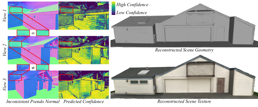
Figure 1: View-Consistent D-Normal Regularizer. Pseudo normals predicted from pretrained monocular normal estimators tend to be inconsistent across different views (left). Our method calculates a confidence map indicating the confidence of the pseudo normals (middle). The confidence is used to weigh the loss imposed on our proposed D-Normals. Our method achieves new state-of-the-art surface reconstruction results and rendering quality comparable with prior work.

1 Introduction

Multi-view stereo (MVS) is a long-standing problem that aims to create 3D surfaces of an object or scene captured from multiple viewpoints [9; 5; 24; 40]. This technique has applications in robotics, graphics, virtual reality, etc. Recently, rendering methods [48; 58; 25] have enhanced the quality of reconstructions. These approaches, often based on implicit neural representations, require extensive training time. For instance, Neuralangelo [25] uses hash encoding [32] for creating high-fidelity surfaces but requires 128 GPU hours for a single scene. On the other hand, the novel 3D Gaussian Spatting method [21] employs 3D Gaussians to render complex scenes photorealistically in real-time, offering a more efficient alternative. Consequently, many recent works attempted the utilization of Gaussian Splatting for surface reconstruction [8; 15; 44; 18]. Although they achieve success in object-level reconstruction, it is still challenging to extract a high-quality surface for large scenes. Previous works [58] improve the surface for scene-level reconstruction by incorporating geometric priors from the off-the-shelf normal estimator. However, there are two main limitations for Gaussian-based reconstruction: 1) Supervising normal rendered from Gaussian Splatting by its nature can only update the rotation parameters, hence failing to update other geometric parameters; 2) The predicted normal maps are inconsistent across multiple views, which may lead to severe reconstruction artifacts.

In this paper, we introduce a novel view-consistent Depth-Normal (D-Normal) regularizer to alleviate the above-mentioned two limitations. For the first limitation, we notice that the supervision of the Gaussian normals can only update its rotations without directly affecting its positions. Consequently, the supervision of Gaussian normals is not as effective as NeuS-based methods [48; 58; 25] whose normal is the gradient of the signed distance function (SDF) that is directly related to the position in 3D space. To solve this issue, we are inspired by the depth and normal estimation [1; 55] to introduce a D-Normal formulation, where the normal is derived from the gradient of rendered depth instead of directly blended from 3D Gaussians. Unlike existing works that obtain depth from the center position of 3D Gaussians, we compute the depth as the intersection of the ray and the compressed Gaussians. Specifically, we first make the Gaussians suitable for 3D reconstruction by applying a scale regularization similar to NeuSG [8] to compress the 3D Gaussian ellipsoids into a plane. Subsequently, the computation of the depth can be simplified to the intersection between a ray and a plane. As a result, our novel parametrization of the depth allows effective full supervision of the Gaussian geometric parameters by any data-driven monocular normal estimator.

To mitigate the inconsistent normal predictions across views, we further propose an uncertainty-aware normal regularizer as shown in Fig. 1. Particularly, we introduce a confidence term for each normal prediction. A high confidence means low uncertainty leading to enhancement of the normal regularization, and vice-versa. Typically, the predicted normal maps from different views are combined to assess the uncertainty of a specific view. However, it is challenging to find correspondence across different views. We circumvent this issue by using the rendered normal learned from multi-view normal priors since we notice that it represents an average of normal priors across views. Furthermore, the confidence term is computed as the cosine distance between the rendered and predicted normals. Although the normal supervision has made the normals more accurate, there is still a minor error leading to depth error arising from the remnant large Gaussians. We thus devise a new densification that splits large Gaussians into smaller ones to represent the surface better. Finally, we incorporate a new splitting strategy to alleviate the surface bumps caused by densification. Experiments show that our approach outperforms Gaussian-based baselines in terms of both reconstruction quality and rendering speed.

Our main contributions are summarized below:

• We formulate a novel multi-view D-Normal regularizer that enables full optimization of the Gaussian geometric parameters to achieve better surface reconstruction.

• We further design a confidence term to weigh our D-Normal regularizer to mitigate inconsistencies of normal predictions across multiple views.

• We introduce a new densification and splitting strategy to alleviate depth error towards more accurate surface modeling.

• Our method outperforms prior work in terms of reconstruction accuracy and running efficiency on the benchmarking Tank and Temples, Replica, MipNeRF360, and DTU datasets.

2 Related Work

Novel View Synthesis. The pursuit of novel view synthesis began with Soft3D [33], which integrated deep learning and volumetric ray-marching to form a continuous, differentiable density field for geometry representation [17; 41]. While effective, this approach was computationally expensive. Neural Radiance Fields (NeRF) [31] improved render quality with importance sampling and positional encoding, but the deep neural networks slowed down processing. Subsequent methods aimed to optimize both quality and speed. Techniques like position encoding and band-limited coordinate networks are combined with neural radiance fields for pre-filtered scene representation [2; 3; 27]. Innovations to speed up rendering included leveraging spatial data structures and adjusting MLP size [6; 11; 14; 16; 34; 43]. Notable examples are InstantNGP [32], which uses a hash grid and a reduced MLP for faster computation, and Plenoxels [11], which employs a sparse voxel grid to eliminate neural networks entirely. Both use Spherical Harmonics to enhance rendering. Despite these advancements, challenges remain in representing empty space and maintaining image quality with structured grids and extensive sampling. Recently, 3D Gaussian Splatting (3DGS) [21] has addressed these issues with unstructured and GPU-optimized splatting, achieving faster and higher-quality rendering without neural components. In this work, we utilize the advantage of Gaussian Splatting to perform surface reconstruction and incorporate normal priors to guide the reconstruction, especially for large indoor and outdoor scenes.

Multi-View Surface Reconstruction. Surface reconstruction is key in 3D vision. Traditional MVS methods [4; 9; 5; 24; 37; 40; 39] use feature matching for depth [4; 37] or voxel-based shapes [9; 5; 24; 40; 45]. Depth-based methods combine depth maps into point clouds, while volumetric methods estimate occupancy and color in voxel grids [9; 5; 28]. However, the finite resolution of voxel grids limits precision. Learning-based MVS modifies traditional steps such as feature matching [30; 47; 59], depth integration [36], or depth inference from images [19; 50; 60; 51; 57]. Further advancements [48; 52] integrated implicit surfaces with volume rendering, achieving detailed surface reconstructions from RGB images. These methods have been extended to large-scale reconstructions via additional regularization [58; 25]. Despite these impressive developments, efficient large-scale scene reconstruction remains a challenge. For example, Neuralangelo [25] requires 128 GPU hours for reconstructing a single scene from the Tanks and Temples Dataset [23]. To accelerate the reconstruction process, some works [15; 18] introduce the 3D Gaussian splitting technique. However, these works still fail in large-scale reconstructions. In this work, we focus on introducing normal regularization for large-scale reconstructions.

3D Gaussian Splatting. Since 3DGS [21] was introduced, it has been rapidly extended to surface reconstruction. We highlight the distinctions between our method and concurrent works SuGaR [15], 2DGS [18], NeuSG [8], and DN-Splatter [46]. In contrast to SuGaR and 2DGS with unsatisfactory performance on large-scale scenes, our method focuses on introducing normal regularization to improve large-scale reconstructions. 2DGS obtaining 2D Gaussian primitives by setting the last entry of scaling factors to zero which is hard to optimize by original Gaussian Splatting technique as noted in  [64; 18], while our method utilizes scale regularization to flatten 3D Gaussians which are easier to optimize. NeuSG utilizes both 3D Gaussian splitting and neural implicit rendering jointly and extracts the surface from an SDF network, while our approach is faster and conceptually simpler by leveraging only Gaussian splatting for surface approximation. Although normal prior is also used for indoor scenes, DN-Splatter may show severe reconstruction artifacts due to their normal supervision can only update the rotation parameters and normal maps inconsistencies across multiple views. Moreover, we do not use the ground truth depth for supervision utilized by DN-Splatter. In comparison, our work is designed to solve both limitations.

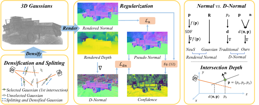
Figure 2: Overview of our VCR-GauS. During densification and splitting, our method only keeps the Gaussians at the first intersections and splits large Gaussians into smaller ones along the major principle axis. The rendered normals are supervised with pseudo normals predicted from a pretrained monocular normal estimator in $\mathcal{L}_{\text{n}}$. We further calculate an uncertainty map based on the discrepancies between the rendered and pseudo normals (cf. Eq. 12) to weigh the loss $\mathcal{L}_{\text{dn}}$ between pseudo normals and D-Normals derived from the rendered depth maps. We compare different approaches for normal calculation (Top Right) and show our intersection depth (Bottom Right).

3 Our Method

Our proposed view-consistent D-Normal regularizer efficiently reconstructs complete and detailed surfaces of scenes from multi-view images. Sec. 3.1 provides an overview of 3D Gaussian Splatting [21]. Our normal and depth formulation of 3D Gaussians is detailed in Sec. 3.2. Sec. 3.3 introduces our proposed regularizations. The densification and splitting of the Gaussian is described in Sec. 3.4. Fig. 2 depicts our whole framework.

3.1 Preliminaries: 3D Gaussian Splatting

3D Gaussian Splatting [21] is an explicit 3D scene representation with 3D Gaussians. Each Gaussian is defined by a covariance matrix $\boldsymbol{\Sigma}$ and a center point $\mathbf{p}\in\mathbb{R}^{3}$ which is the mean of the Gaussian. The 3D Gaussian distribution can be represented as:

$$G(\mathbf{x})=\exp{\{-\frac{1}{2}(\mathbf{x}-\mathbf{p})^{\top}\boldsymbol{\Sigma}^{-1}(\mathbf{x}-\mathbf{p})\}}.$$ (1)

To maintain positive semi-definiteness during optimization, the covariance matrix $\boldsymbol{\Sigma}$ is expressed as the product of a scaling matrix $\mathbf{S}$ and a rotation matrix $\mathbf{R}$:

$$\boldsymbol{\Sigma}=\mathbf{R}\mathbf{S}\mathbf{S}^{\top}\mathbf{R}^{\top},$$ (2)

where $\mathbf{S}$ is a diagonal matrix, stored by a scaling factor $\mathbf{s}\in\mathbb{R}^{3}$, and the rotation matrix $\mathbf{R}$ is represented by a quaternion $\mathbf{r}\in\mathbb{R}^{4}$.

For novel view rendering, the splatting technique [54] is applied to the Gaussians on the camera planes. Using the viewing transform matrix $\mathbf{W}$ and the Jacobian of the affine approximation of the projective transformation $\mathbf{J}$ [63], the transformed covariance matrix $\boldsymbol{\Sigma}^{\prime}$ can be determined as:

$$\boldsymbol{\Sigma}^{\prime}=\mathbf{J}\mathbf{W}\boldsymbol{\Sigma}\mathbf{W}^{\top}\mathbf{J}^{\top}.$$ (3)

A 3D Gaussian is defined by its position $\mathbf{p}$, quaternion $\mathbf{r}$, scaling factor $\mathbf{s}$, opacity $\alpha\in\mathbb{R}$, and color represented with spherical harmonics coefficients $\mathbf{H}\in\mathbb{R}^{k}$. For a given pixel, the combined color and opacity from multiple Gaussians are weighted by Eq. 1. The color blending for overlapping points is:

$$\hat{\mathbf{C}}=\sum_{i\in M}\mathbf{c}_{i}\alpha_{i}\prod_{j=1}^{i-1}(1-\alpha_{j}),$$ (4)

where $\mathbf{c}_{i}$ and $\alpha_{i}$ denote the color and density of a point, respectively.

3.2 Geometric Properties

To reconstruct the 3D surface, we introduce two geometric properties: normal and depth of a Gaussian, which are used to render the corresponding normal map and depth map for regularization.

Normal Vector. Following NeuSG [8], the normal of the Gaussian can be represented as the direction of the minimized scaling factor. The normal in the world coordinate system is defined as:

$$\mathbf{n}=\mathbf{R}[k,:]\in\mathbb{R}^{3},k=\operatorname{argmin}\left(\left[s_{1},s_{2},s_{3}\right]\right),$$ (5)

The normal n and position p are transformed into the camera coordination system with the camera extrinsic matrix, which we subsequently take as the default unless otherwise stated.

Intersection Depth. The existing work [44] obtains the depth from the center position $\textbf{p}=(p_{x},p_{y},p_{z})$ of each Gaussian in the camera coordinate system. However, this formulation is inaccurate and results in the depth from each Gaussian center being unrelated to its normal n during optimization. A more reasonable depth calculation is to compute the depth of the intersection between the Gaussian and the ray emitted from the camera center. To simplify the computation of intersection and represent the surface, we incorporate a scale regularization loss $\mathcal{L}_{\text{scale}}$ from NeuSG [8] to squeeze the 3D Gaussian ellipsoids into highly flat shapes. This loss constrains the minimum component of the scaling factor $\mathbf{s}=(s_{1},s_{2},s_{3})^{\top}\in\mathbb{R}^{3}$ for each Gaussian towards zero:

$$\mathcal{L}_{\text{s}}=\|\min(s_{1},s_{2},s_{3})\|_{1}.$$ (6)

This process effectively flattens the 3D Gaussian towards a planar shape which we represent by $(\textbf{p},\textbf{n})$. As a result, any point $\textbf{o}_{p}$ on the plane follows the incidence equation given by: $\textbf{n}\cdot(\textbf{o}_{p}-\textbf{p})=0$. We further denote any point $\textbf{o}_{l}$ on a ray that passes through the origin in 3D space as $\textbf{o}_{l}=\textbf{r}t$, where $t\in\mathbb{R}$ is the distance from the point to the origin along the ray. We set $\textbf{o}_{l}=\textbf{o}_{p}$ at the intersection of the ray with the plane, which we can then solve for the depth of the intersection along the $z$-axis as:

$$d(\mathbf{n},\mathbf{p})=\mathbf{r}_{z}*(\mathbf{n}\cdot\mathbf{p})/(\mathbf{n}\cdot\mathbf{r}),$$ (7)

where $\mathbf{r}_{z}$ is the z-value of the ray direction r. From the equation, we can see the intersection depth is related to both the position p and the normal n of the Gaussian. This not only offers more accurate depth calculation but also enables the D-Normal regularization to backpropagate its loss to all different Gaussian parameters.

3.3 View-Consistent D-Normal Regularization

We first introduce our D-Normal formulation to allow the full optimization of the Gaussian geometric parameters. We further propose a confidence term to relieve the constraint from uncertain predictions and strengthen it from certain ones to avoid the wrong guidance from the inconsistent normal priors from a pretrained monocular model across multiple views.

D-Normal Regularizer. To improve the reconstruction quality, we utilize a normal prior N predicted from a pretrained monocular deep neural network [1] to supervise the rendered normal map $\hat{\mathbf{N}}$ with L1 and cosine losses:

$$\mathcal{L}_{\text{n}}=\|\hat{\textbf{N}}-\textbf{N}\|_{1}+(1-\hat{\textbf{N}}\cdot\textbf{N}),$$ (8)

where the rendered normal map $\hat{\mathbf{N}}$ applies weighted-sum normal, different from color rendering using alpha blending. However, normal regularization alone is insufficient for surface reconstruction as compared with NeuS-based methods. As illustrated in Fig. 2, NeuS-based methods compute normals as the gradients of the SDF function calculated from input position p, and therefore the regularization of normal can affect the position directly. However, the normal is only directly related to the rotation of the Gaussian during Gaussian splitting, which means directly supervising the rendered normals cannot update the positions as shown in Fig. 2. To solve this problem and inspired by normal and depth estimation [1; 55], we propose a new depth-normal formulation. First, we render the depth map by weighted summing the depths:

$$\hat{D}={\sum_{i\in M}d_{i}\alpha_{i}\prod_{j=1}^{i-1}(1-\alpha_{j})}/{\sum_{i\in M}\alpha_{i}\prod_{j=1}^{i-1}(1-\alpha_{j})},$$ (9)

where $d_{i}$ is the intersection depth from Eq. 7. Subsequently, we convert the rendered depth $\hat{D}$ to a D-Normal $\bar{\textbf{N}}_{d}$ and use the predicted normal N by a pretrained model to supervise the depth via the D-Normal $\bar{\textbf{N}}_{d}$. In particular, the D-Normal is computed by back-projecting the depth map into point clouds $\{\textbf{d}_{k}(\textbf{n},\textbf{p})\}$ with the camera intrinsic matrix. The D-Normal $\bar{\textbf{N}}_{d}$ is then computed by the cross-product with the horizontal and vertical finite differences from the neighboring points:

$$\bar{\textbf{N}}_{d}(\textbf{n},\textbf{p})=\frac{\nabla_{v}\mathbf{d}(\textbf{n},\textbf{p})\times\nabla_{h}\mathbf{d}(\textbf{n},\textbf{p})}{|\nabla_{v}\mathbf{p}(\textbf{n},\textbf{p})\times\nabla_{h}\mathbf{d}(\textbf{n},\textbf{p})|}.$$ (10)

From this equation, we can see the D-Normal is a function of both the normal n and the position p of Gaussians. This allows the regularization on the D-Normal to optimize both normal n and position p. The D-Normal regularization is formulated as:

$$\mathcal{L}_{\text{dn}}=\|\bar{\textbf{N}}_{d}-\textbf{N}\|_{1}+(1-\bar{\textbf{N}}_{d}\cdot\textbf{N}).$$ (11)

Confidence. Although the D-Normal regularizer resolves the issue with the Gaussian position in the supervision of its normal, the normal maps predicted by a pretrained model are not always accurate. This is especially problematic when inconsistencies arise across multiple views. We thus introduce a confidence term $w$ to emphasize the regularization for high certainty areas while reducing on low certainty areas. Typically, the normals from different views are combined to assess the certainty of a specific view. However, it is challenging to find correspondence between different views. We circumvent the challenge by using the rendered normal learned from multi-view pseudo normals, which represents an average of the pseudo normals across the views. As a result, we can use the rendered normal to gauge the uncertainty of the predicted normal in the current view. Specifically, the confidence term $w$ is computed as the cosine distance between the rendered and predicted normals, i.e.:

$$w=\exp\{(\bar{\textbf{N}}_{d}\cdot\textbf{N}-1)/\gamma\},$$ (12)

where $\gamma$ is a hyper-parameter. Consequently, the view-consistent D-Normal regularizer is defined as:

$$\mathcal{L}_{\text{dn}}=w*(\|\bar{\textbf{N}}_{d}-\textbf{N}\|_{1}+(1-\bar{\textbf{N}}_{d}\cdot\textbf{N})).$$ (13)

The overall loss function combining these elements is:

$$\mathcal{L}_{\text{total}}=\mathcal{L}_{\text{RGB}}+\lambda_{1}\mathcal{L}_{\text{s}}+\lambda_{2}\mathcal{L}_{\text{n}}+\lambda_{3}\mathcal{L}_{\text{dn}},$$ (14)

with $\lambda_{1}$, $\lambda_{2}$ and $\lambda_{3}$ balancing the individual components. $\mathcal{L}_{\text{RGB}}$ includes L1 and D-SSIM losses.

3.4 Densification and Splitting

We observe that the original densification and splitting in Gaussian Splatting causes depth error as well as surface bumps and protrusions to appear. To address this issue, we further propose a new densification and splitting strategy as depicted in Fig. 2 (Bottom Left).

Densification. Although normal supervision has made the normals more accurate, there is still a minor error $\theta$ leading to depth error arising from the remnant large Gaussians since Gaussian size is not the consideration in the original “large position gradient" selection criteria for Gaussians to be densified. As illustrated in Fig. 3(a), a very small normal error at the edges can result in a significant depth error $\sin\theta\cdot r$ away from the center for larger Gaussians (top of figure). Comparatively, the depth error is small for smaller Gaussians since $r^{\prime}$ becomes relatively smaller (bottom of figure). Consequently, we subdivide the larger Gaussians into smaller Gaussians to keep the depth error small. To achieve this, we first randomly sample camera views from a cuboid that encompasses the entire scene for object-centric outdoor scenes and from the training views for indoor scenes. Since we aim to densify only the surface Gaussians, we only keep the first intersected Gaussian and discard the rest for each ray emitted from the camera. Subsequently, we densify only those with a scale above a threshold $\beta$ among the collected Gaussians.

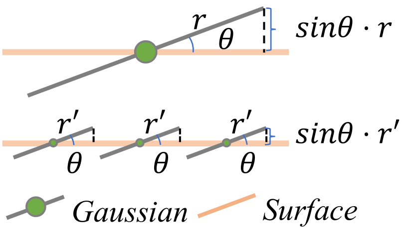
(a) Large vs. Small Gaussians

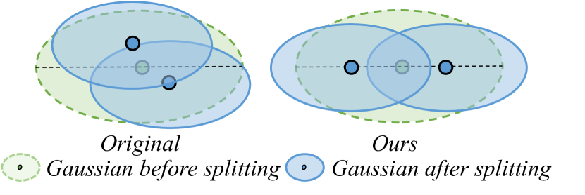
(b) Splitting Strategy

Figure 3: Illustration of the rationals behind the densification and splitting strategies. (a) Comparison between large and small Gaussians of depth errors caused by a small normal error (in side view). (b) Comparison of the original and the proposed splitting strategies (in bird-eye view).

Splitting. We notice that the Gaussians tend to protrude the ground truth surface after densification due to the clustering of many Gaussians. As also observed in Mip-Splatting [56], Gaussians splitted from the same parents tend to remain clustered with relatively stable positions due to the sampling from the same Gaussian distribution. To avoid clustering, we split the old Gaussian into two new Gaussian along the axis with the largest scale instead of using the Gaussian sampling with the position of the Gaussian as mean and the 3D scale of the Gaussian as variance. The positions of the new Gaussians evenly divide the maximum scale of the old Gaussian. Other parameters of new Gaussians are obtained following the original 3DGS. This process is shown in Fig. 3(b).

4 Experiments

Table 1: Quantitative results on the Tanks and Temples Dataset [23]. Reconstructions are evaluated with the official evaluation scripts and we report F1-score, average optimization time and FPS. Ours outperforms all 3DGS-based surface reconstruction methods by a large margin and performs better than neural implicit methods by a minor margin while optimizing significantly faster.

	NeuS-based			Gaussian-based
	NeuS	MonoSDF	Geo-Neus	SuGaR	3DGS	2DGS	Ours
Barn	0.29	0.49	0.33	0.14	0.13	0.36	0.62
Caterpillar	0.29	0.31	0.26	0.16	0.08	0.23	0.26
Courthouse	0.17	0.12	0.12	0.08	0.09	0.13	0.19
Ignatius	0.83	0.78	0.72	0.33	0.04	0.44	0.61
Meetingroom	0.24	0.23	0.20	0.15	0.01	0.16	0.19
Truck	0.45	0.42	0.45	0.26	0.19	0.26	0.52
Mean	0.38	0.39	0.35	0.19	0.09	0.30	0.40
Time	>24h	>24h	>24h	>1h	14.3 m	34.2 m	53 m
FPS	<10			-	159	68	145

We first evaluate our method on 3D surface reconstruction in Sec. 4.1. We also report the rendering results in Sec. 3. Additionally, we validate the effectiveness of the proposed techniques in Sec. 4.2.

Figure 4: Qualitative comparison on TNT dataset. From top to bottom, we show the reconstructed meshes from our method, SuGar, 2DGS, and NeuS, as well as the ground truth colored point cloud. Our method reconstructs more complete surfaces featuring smoother planar regions and finer details.

Dataset. We evaluate the performance of our method on various datasets. For surface reconstruction, we evaluate on Tanks and Temples (TNT) [23]. To further validate the effectiveness of our method, we compare with other methods on Replica [42]. Although we focus on the large-scale reconstruction, we also report our results on DTU [20], which can be seen in the supplementary. Furthermore, we evaluate the rendering results on Mip-NeRF360 [3]. For all the datasets, we use COLMAP [38] to generate a sparse point cloud for each scene as initialization.

Implementation Details. Our method is built upon the open-source 3DGS code base [21] and the intersection depth calculation is implemented with custom CUDA kernels. $\lambda_{1}$, $\lambda_{2}$, and $\lambda_{3}$ are set to $1$, $0.01$, and $0.015$, respectively. The densification threshold $\beta$ is set to $0.002$. The hyperparameter $\gamma$ is set to $0.005$. We use pretrained DSINE [1] to predict normal maps for outdoor scenes and pretrained GeoWizard [13] for indoor scenes. We also employ a semantic surface trimming approach to avoid unwanted background elements like the sky in the reconstructions for outdoor scenes, which is introduced in the supplementary material. Similar to 3DGS, we stop densification at 15k iterations and optimize all of our model parameters for 30k iterations. For mesh extraction, we adapt truncated signed distance fusion (TSDF) to fuse the rendered depth maps using Open3D [62].

4.1 Comparison

Table 2: Quantitative assessment on Replica [42]. Bold indicates the best.

	Method	F1-score	Time
Implicit	NeuS	65.12	$>$10h
	MonoSDF	81.64
Explicit	3DGS	50.79	$\leq$1h
	SuGar	63.20
	2DGS	64.36
	Ours	78.17

Surface Reconstruction. As shown in Tab. 1, our method outperforms SDF models (i.e., NeuS [48], MonoSDF [58], and Geo-NeuS [12]) on the TNT dataset, and reconstructs significantly better surfaces than explicit reconstruction methods (i.e., 3DGS [21], SuGaR [15], and 2DGS [18]). Notably, our model demonstrates exceptional efficiency, offering a reconstruction speed that is approximately 20 times faster compared to NeuS-based reconstruction methods. Compared with the concurrent work 2DGS[18], although our method is a little slower than it (about 20 minutes), it works much better (0.3 vs. 0.4). As shown in  Fig. 4, our approach better recovers planar surfaces (e.g., roof in Barn and ground in Truck) as well as finer geometry details. In addition, 2DGS renders much slower than ours (68 FPS vs. 145 FPS). On the Replica dataset shown in Tab. 2, our method is much faster than MonoSDF (10+ hours vs.  50 minutes) although showing comparable performance. Compared with explicit reconstruction methods, including 3DGS, SuGaR, and 2DGS, our method achieves significantly higher F1-score for reconstruction. Although we focus on large-scale reconstruction, we also report the results on object-level reconstruction DTU [20] (cf. supplementary).

Table 3: Quantitative results on Mip-NeRF 360 [3]. Our method achieves NVS rendering quality and speed comparable with other Gaussian-based methods.

	Outdoor Scene			Indoor Scene			FPS $\uparrow$
	PSNR $\uparrow$	SSIM $\uparrow$	LPIPS $\downarrow$	PSNR $\uparrow$	SSIM $\uparrow$	LIPPS $\downarrow$
NeRF	21.46	0.458	0.515	26.84	0.790	0.370	<10
Deep Blending	21.54	0.524	0.364	26.40	0.844	0.261
Instant NGP	22.90	0.566	0.371	29.15	0.880	0.216
MERF	23.19	0.616	0.343	27.80	0.855	0.271
MipNeRF360	24.47	0.691	0.283	31.72	0.917	0.180
Mobile-NeRF	21.95	0.470	0.470	-	-	-	<100
BakedSDF	22.47	0.585	0.349	27.06	0.836	0.258
3DGS	24.64	0.731	0.234	30.41	0.920	0.189	134
SuGaR	22.93	0.629	0.356	29.43	0.906	0.225	-
2DGS	24.21	0.709	0.276	30.10	0.913	0.211	27
Ours	24.31	0.707	0.280	30.53	0.921	0.184	128

Novel View Synthesis. Our method can reconstruct 3D surfaces and provide high-quality novel view synthesis. As shown in Tab. 3, we compare our novel view rendering results against baseline approaches on the Mip-NeRF360 dataset in this section. Remarkably, our method consistently achieves competitive novel view synthesis results compared to state-of-the-art techniques (e.g., Mip-NeRF360, 3DGS, etc.) while providing geometrically accurate surface reconstruction. Furthermore, our method renders a few times faster than the concurrent work 2DGS (128 FPS vs. 27 FPS). The reason is that our method utilizes the original and efficient Gaussian Splatting technique, while 2DGS applies a time-consuming ray-splat technique.

4.2 Ablation Studies

Table 4: Ablation on TNT [23]. Bold indicates best result.

Ablation Item	Precision $\uparrow$	Recall $\uparrow$	F-score $\uparrow$
A. w/o D-Normal	0.27	0.34	0.30
B. w/o confidence	0.36	0.37	0.36
C. w/o intersection depth	0.35	0.37	0.35
D. w/o densify and split	0.32	0.35	0.33
E. Full	0.39	0.42	0.40

We verify the effectiveness of different design choices on reconstruction quality, including regularization terms, intersection depth, and densification on the TNT dataset [23] and report the F1-score. We first examine the effect of our view-consistent D-Normal regularization. Our full model (Tab. 4 E) provides the best performance (0.40 F1-score). The performance drops 0.10 F1-score from 0.4 to 0.3 without the D-Normal regularizer (Tab. 4 A) while keeping rendered normal regularization. It proves that it is insufficent to supervise only the normal maps rendered from Gaussian Splatting. Furthermore, the result drops by 0.04 F1-score without the confidence (Tab. 4 B) and with the D-Normal regularizer. It demonstrates that confidence can mitigate the problem of inconsistency of the predicted normal maps. From Fig. 5, we can observe that disabling the confidence leads to an unsmooth surface. Both of these validate the effectiveness of the view-consistent D-Normal regularization. Additionally, the absence of intersection depth (Tab. 4 C) results in poor performance. Lastly, the performance increases from 0.33 F1-score to 0.40 with our densification and split (Tab. 4 D), proving small Gaussians represent surfaces better than large Gaussians.

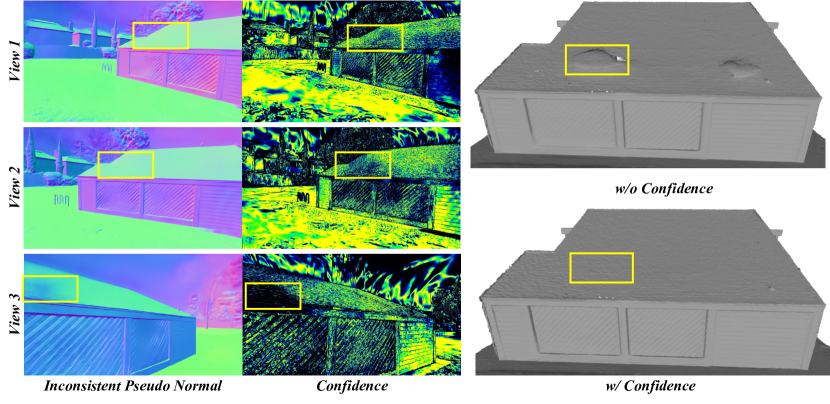
Figure 5: Qualitative ablation for the confidence. Without the confidence weight, the reconstructed surface shows protrusions caused by the inconsistent pseudo normal maps across different views.

5 Conclusion

In this work, we have introduced a view-consistent D-Normal regularizer for efficient, high-quality, and compact surface reconstruction. We formulate the D-Normal regularizer that directly couples normal with the other geometric parameters. This allows for the full update of all geometric parameters during normal regularization. We also propose a confidence term that weighs our D-Normal regularizer to mitigate inconsistencies of normal predictions across multiple views. Finally, we introduce a densification and splitting strategy to regularize the scales and distribution of 3D Gaussians for more precise surface modeling. Our evaluations on diverse datasets demonstrate that our method outperforms existing works in surface reconstruction.

Appendix A Supplemental Material

A.1 Semantic Surface Trimming

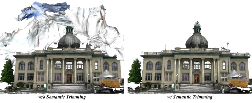
Figure 6: Qualitative ablation for the semantic trimming. The left is disabling the semantic trimming and the right is enabling the strategy. We can see that the proposed semantic trimming can prune the unwanted regions, like the sky in the left figure.

To avoid unwanted background elements like the sky in reconstructions for outdoor scenes, we employ a semantic surface trimming approach by learning a semantic field [53, 7, 49, 61] that leverages a pretrained semantic model [22, 29, 35]. Specifically, we assign each Gaussian with a learnable semantic feature. Subsequently, similar to color blending, alpha blending is applied on these features to get the pixel-level semantics. We use the predicted semantic map from Grounded-SAM [35] with cross-entropy loss to train the learnable features. After the optimization, we render the semantic map for each view and then use the semantics to mask out the background. Although we can use the predicted semantic maps from Grounded-SAM to prune the background directly, the predicted semantic maps are not always accurate and consistent across views. Our proposed method can get a more accurate semantics with noisy pseudo labels to a certain extent, which is also observed in [61].

A.2 Implementation Details

We use PyTorch 2.0.1 and CUDA 11.8. for most experiments. All experiments are conducted on an NVIDIA 3090/4090/A5000/A6000 GPU. We set most hyperparameters to the same as that used in Gaussian Splatting [21]. For outdoor scenes in the TNT dataset, we also utilize decoupled appearance modeling [26] to alleviate the exposure issue. Moreover, to remove some outlier Gaussians, we adopt a pruning technique from LightGaussian [10]. We also use a cuboid bounding box to contain the scene we need to reconstruct and we only regulate and add the new densification to Gaussians inside the box. We use the same train and test data with 2DGS on TNT, Mip-NeRF360, and DTU datasets.

Table 5: Additional ablation on TNT Dataset.

	Precision $\uparrow$	Recall $\uparrow$	F-score $\uparrow$
F. w/o semantic trimming	0.37	0.42	0.38
G. w/o scale regularization	0.35	0.38	0.36
H. Set scale $s_{3}$ zero	0.36	0.40	0.37
I. Scale Regularization	0.39	0.42	0.40

A.3 Additional Ablation Studies

We further verify the effectiveness of additional design choices on reconstruction quality. We conduct experiments on the TNT dataset [23] and report the F1-score. The quantitative result is reported in Tab. 5. We first verify the proposed semantic trimming strategy (Tab. 5 F). From the table, we can see the strategy can increase the F1-score by 0.02. We can also observe the qualitative result from Fig. 6 that the trimming strategy can prune the sky correctly. Additionally, we confirm the effectiveness of scale regularization (Tab. 5 G), which leads to an improvement of 0.04. The current work [18] sets the last item of the scale factor to zero to flatten the 3D Gaussians for surface reconstruction. Additionally, we also ablate the setting zero (Tab. 5 H) and the scale regularization (Tab. 5 I). From the table, we can see that using the scale regularization instead of setting zero can obtain a 0.03 F1-score improvement.

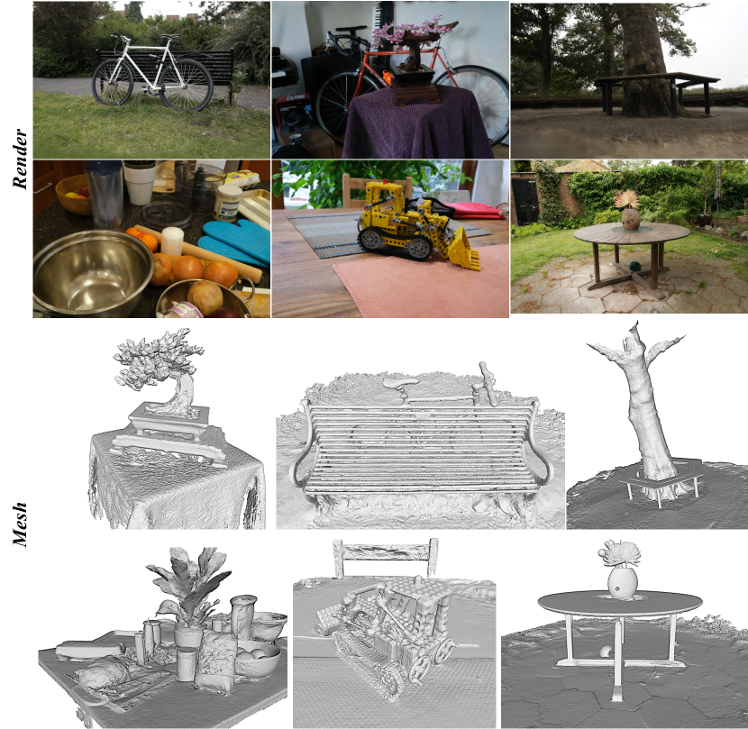
Figure 7: Qualitative results on the Mip-NeRF360 dataset. Our method reconstructs surfaces with fine geometry details and produces high-fidelity renderings on Mip-NeRF360 dataset.

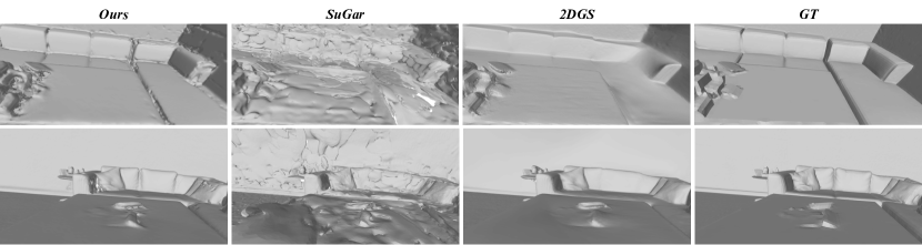
Figure 8: Qualitative results on the Replica dataset.

A.4 Additional Qualitative Results

Fig. 7 shows the rendering (top) and reconstruction (down) results on the Mip-NeRF360 [2] dataset. The rendering results on the TNT and Replica datasets are shown in Fig. 9. We also compare the qualitative results of VCR-GauS with SuGar and 2DGS, shown in Fig. 8. From the figure, we can see that our method can reconstruct both complete and high-detailed surfaces. In addition to the visualization in the form of pictures, we have also recorded a video in the supplementary material that can be downloaded and watched.

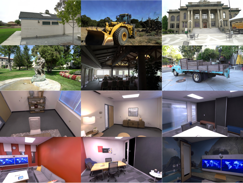
Figure 9: Qualitative rendering results on the TNT and Replica dataset.

A.5 Additional Dataset

Table 6: Quantitative comparison on the DTU Dataset [20]. We show the Chamfer distance and average optimization time.

Method			24	37	40	55	63	65	69	83	97	105	106	110	114	118	122		Mean	Time
Implicit	NeRF [31]		1.90	1.60	1.85	0.58	2.28	1.27	1.47	1.67	2.05	1.07	0.88	2.53	1.06	1.15	0.96		1.49	>12h
	VolSDF [52]		1.14	1.26	0.81	0.49	1.25	0.70	0.72	1.29	1.18	0.70	0.66	1.08	0.42	0.61	0.55		0.86	>12h
	NeuS [48]		1.00	1.37	0.93	0.43	1.10	0.65	0.57	1.48	1.09	0.83	0.52	1.20	0.35	0.49	0.54		0.84	>12h
	MonoSDF [58]		0.83	1.61	0.65	0.47	0.92	0.87	0.87	1.30	1.25	0.68	0.65	0.96	0.41	0.62	0.58		0.84	>12h
Explicit	3DGS [21]		2.14	1.53	2.08	1.68	3.49	2.21	1.43	2.07	2.22	1.75	1.79	2.55	1.53	1.52	1.50		1.96	< 1h
	SuGaR [15]		1.47	1.33	1.13	0.61	2.25	1.71	1.15	1.63	1.62	1.07	0.79	2.45	0.98	0.88	0.79		1.33	< 1h
	2DGS [18]		0.48	0.91	0.39	0.39	1.01	0.83	0.81	1.36	1.27	0.76	0.70	1.40	0.40	0.76	0.52		0.80	< 1h
	Ours		0.55	0.91	0.40	0.43	0.97	0.95	0.84	1.39	1.30	0.90	0.76	0.92	0.44	0.75	0.54		0.80	< 1h

In this section, we report the result of object-level reconstruction. Although we focus on large-scale reconstruction, we still outperform implicit (i.e., NeRF, VolSDF, NeuS, and MonoSDF) and most explicit methods (i.e., 3DGS and SuGaR) on DTU [20]. While our method is comparable with current work 2DGS on object-level reconstruction, our method is much better than it on large-scale reconstruction, as shown in Tab. 1 and Tab. 2. The qualitative results on DTU are shown in Fig. 10.

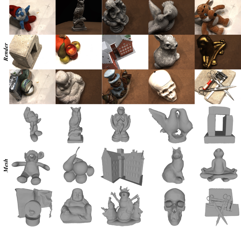
Figure 10: Qualitative results on the DTU dataset.

Appendix B Limitations

Although our method can alleviate the problem of inaccurate normal prediction from a pretrained normal estimator, especially the inconsistent normal predictions across views, it fails under the extreme case when almost all predicted normal across views are wrong. In addition, our method cannot reconstruct beyond the observed scene. Furthermore, our method cannot capture the surface of the semi-transparent object, shown in Fig. 11.

Figure 11: Illustration of limitations: Our VCR-GauS encounters difficulties in accurately reconstructing semi-transparent surfaces, such as the window depicted in Caterpillar.

References

- [1] Gwangbin Bae and Andrew J. Davison. Rethinking inductive biases for surface normal estimation. In IEEE/CVF Conference on Computer Vision and Pattern Recognition (CVPR), 2024.
- [2] Jonathan T Barron, Ben Mildenhall, Matthew Tancik, Peter Hedman, Ricardo Martin-Brualla, and Pratul P Srinivasan. Mip-nerf: A multiscale representation for anti-aliasing neural radiance fields. In Proceedings of the IEEE/CVF International Conference on Computer Vision, pages 5855–5864, 2021.
- [3] Jonathan T Barron, Ben Mildenhall, Dor Verbin, Pratul P Srinivasan, and Peter Hedman. Mip-nerf 360: Unbounded anti-aliased neural radiance fields. In Proceedings of the IEEE/CVF Conference on Computer Vision and Pattern Recognition, pages 5470–5479, 2022.
- [4] Michael Bleyer, Christoph Rhemann, and Carsten Rother. Patchmatch stereo-stereo matching with slanted support windows. In Bmvc, volume 11, pages 1–11, 2011.
- [5] Adrian Broadhurst, Tom W Drummond, and Roberto Cipolla. A probabilistic framework for space carving. In Proceedings eighth IEEE international conference on computer vision. ICCV 2001, volume 1, pages 388–393. IEEE, 2001.
- [6] Anpei Chen, Zexiang Xu, Andreas Geiger, Jingyi Yu, and Hao Su. Tensorf: Tensorial radiance fields. In European Conference on Computer Vision, pages 333–350. Springer, 2022.
- [7] Hanlin Chen, Chen Li, Mengqi Guo, Zhiwen Yan, and Gim Hee Lee. Gnesf: Generalizable neural semantic fields. In Thirty-seventh Conference on Neural Information Processing Systems, 2023.
- [8] Hanlin Chen, Chen Li, and Gim Hee Lee. Neusg: Neural implicit surface reconstruction with 3d gaussian splatting guidance. arXiv preprint arXiv:2312.00846, 2023.
- [9] Jeremy S De Bonet and Paul Viola. Poxels: Probabilistic voxelized volume reconstruction. In Proceedings of International Conference on Computer Vision (ICCV), volume 2, page 2. Citeseer, 1999.
- [10] Zhiwen Fan, Kevin Wang, Kairun Wen, Zehao Zhu, Dejia Xu, and Zhangyang Wang. Lightgaussian: Unbounded 3d gaussian compression with 15x reduction and 200+ fps, 2023.
- [11] Sara Fridovich-Keil, Alex Yu, Matthew Tancik, Qinhong Chen, Benjamin Recht, and Angjoo Kanazawa. Plenoxels: Radiance fields without neural networks. In Proceedings of the IEEE/CVF Conference on Computer Vision and Pattern Recognition, pages 5501–5510, 2022.
- [12] Qiancheng Fu, Qingshan Xu, Yew Soon Ong, and Wenbing Tao. Geo-neus: Geometry-consistent neural implicit surfaces learning for multi-view reconstruction. Advances in Neural Information Processing Systems, 35:3403–3416, 2022.
- [13] Xiao Fu, Wei Yin, Mu Hu, Kaixuan Wang, Yuexin Ma, Ping Tan, Shaojie Shen, Dahua Lin, and Xiaoxiao Long. Geowizard: Unleashing the diffusion priors for 3d geometry estimation from a single image. arXiv preprint arXiv:2403.12013, 2024.
- [14] Stephan J Garbin, Marek Kowalski, Matthew Johnson, Jamie Shotton, and Julien Valentin. Fastnerf: High-fidelity neural rendering at 200fps. In Proceedings of the IEEE/CVF International Conference on Computer Vision, pages 14346–14355, 2021.
- [15] Antoine Guédon and Vincent Lepetit. Sugar: Surface-aligned gaussian splatting for efficient 3d mesh reconstruction and high-quality mesh rendering. In IEEE/CVF Conference on Computer Vision and Pattern Recognition (CVPR), 2024.
- [16] Peter Hedman, Pratul P Srinivasan, Ben Mildenhall, Jonathan T Barron, and Paul Debevec. Baking neural radiance fields for real-time view synthesis. In Proceedings of the IEEE/CVF International Conference on Computer Vision, pages 5875–5884, 2021.
- [17] Philipp Henzler, Niloy J Mitra, and Tobias Ritschel. Escaping plato’s cave: 3d shape from adversarial rendering. In Proceedings of the IEEE/CVF International Conference on Computer Vision, pages 9984–9993, 2019.
- [18] Binbin Huang, Zehao Yu, Anpei Chen, Andreas Geiger, and Shenghua Gao. 2d gaussian splatting for geometrically accurate radiance fields. SIGGRAPH, 2024.
- [19] Po-Han Huang, Kevin Matzen, Johannes Kopf, Narendra Ahuja, and Jia-Bin Huang. Deepmvs: Learning multi-view stereopsis. In Proceedings of the IEEE Conference on Computer Vision and Pattern Recognition, pages 2821–2830, 2018.
- [20] Rasmus Jensen, Anders Dahl, George Vogiatzis, Engil Tola, and Henrik Aanæs. Large scale multi-view stereopsis evaluation. In 2014 IEEE Conference on Computer Vision and Pattern Recognition, pages 406–413. IEEE, 2014.
- [21] Bernhard Kerbl, Georgios Kopanas, Thomas Leimkühler, and George Drettakis. 3d gaussian splatting for real-time radiance field rendering. ACM Transactions on Graphics, 42(4), July 2023.
- [22] Alexander Kirillov, Eric Mintun, Nikhila Ravi, Hanzi Mao, Chloe Rolland, Laura Gustafson, Tete Xiao, Spencer Whitehead, Alexander C. Berg, Wan-Yen Lo, Piotr Dollár, and Ross Girshick. Segment anything. arXiv:2304.02643, 2023.
- [23] Arno Knapitsch, Jaesik Park, Qian-Yi Zhou, and Vladlen Koltun. Tanks and temples: Benchmarking large-scale scene reconstruction. ACM Transactions on Graphics (ToG), 36(4):1–13, 2017.
- [24] Kiriakos N Kutulakos and Steven M Seitz. A theory of shape by space carving. International journal of computer vision, 38:199–218, 2000.
- [25] Zhaoshuo Li, Thomas Müller, Alex Evans, Russell H Taylor, Mathias Unberath, Ming-Yu Liu, and Chen-Hsuan Lin. Neuralangelo: High-fidelity neural surface reconstruction. In IEEE Conference on Computer Vision and Pattern Recognition (CVPR), 2023.
- [26] Jiaqi Lin, Zhihao Li, Xiao Tang, Jianzhuang Liu, Shiyong Liu, Jiayue Liu, Yangdi Lu, Xiaofei Wu, Songcen Xu, Youliang Yan, and Wenming Yang. Vastgaussian: Vast 3d gaussians for large scene reconstruction. In CVPR, 2024.
- [27] David B Lindell, Dave Van Veen, Jeong Joon Park, and Gordon Wetzstein. Bacon: Band-limited coordinate networks for multiscale scene representation. In Proceedings of the IEEE/CVF conference on computer vision and pattern recognition, pages 16252–16262, 2022.
- [28] Shaohui Liu, Yinda Zhang, Songyou Peng, Boxin Shi, Marc Pollefeys, and Zhaopeng Cui. Dist: Rendering deep implicit signed distance function with differentiable sphere tracing. In Proceedings of the IEEE/CVF Conference on Computer Vision and Pattern Recognition, pages 2019–2028, 2020.
- [29] Shilong Liu, Zhaoyang Zeng, Tianhe Ren, Feng Li, Hao Zhang, Jie Yang, Chunyuan Li, Jianwei Yang, Hang Su, Jun Zhu, et al. Grounding dino: Marrying dino with grounded pre-training for open-set object detection. arXiv preprint arXiv:2303.05499, 2023.
- [30] Wenjie Luo, Alexander G Schwing, and Raquel Urtasun. Efficient deep learning for stereo matching. In Proceedings of the IEEE conference on computer vision and pattern recognition, pages 5695–5703, 2016.
- [31] Ben Mildenhall, Pratul Srinivasan, Matthew Tancik, Jonathan Barron, Ravi Ramamoorthi, and Ren Ng. Nerf: Representing scenes as neural radiance fields for view synthesis. In European Conference on Computer Vision, pages 405–421. Springer, 2020.
- [32] Thomas Müller, Alex Evans, Christoph Schied, and Alexander Keller. Instant neural graphics primitives with a multiresolution hash encoding. ACM Transactions on Graphics (ToG), 41(4):1–15, 2022.
- [33] Eric Penner and Li Zhang. Soft 3d reconstruction for view synthesis. ACM Transactions on Graphics (TOG), 36(6):1–11, 2017.
- [34] Christian Reiser, Songyou Peng, Yiyi Liao, and Andreas Geiger. Kilonerf: Speeding up neural radiance fields with thousands of tiny mlps. In Proceedings of the IEEE/CVF International Conference on Computer Vision, pages 14335–14345, 2021.
- [35] Tianhe Ren, Shilong Liu, Ailing Zeng, Jing Lin, Kunchang Li, He Cao, Jiayu Chen, Xinyu Huang, Yukang Chen, Feng Yan, Zhaoyang Zeng, Hao Zhang, Feng Li, Jie Yang, Hongyang Li, Qing Jiang, and Lei Zhang. Grounded sam: Assembling open-world models for diverse visual tasks, 2024.
- [36] Gernot Riegler, Ali Osman Ulusoy, Horst Bischof, and Andreas Geiger. Octnetfusion: Learning depth fusion from data. In 2017 International Conference on 3D Vision (3DV), pages 57–66. IEEE, 2017.
- [37] Johannes L Schönberger, Enliang Zheng, Jan-Michael Frahm, and Marc Pollefeys. Pixelwise view selection for unstructured multi-view stereo. In Computer Vision–ECCV 2016: 14th European Conference, Amsterdam, The Netherlands, October 11-14, 2016, Proceedings, Part III 14, pages 501–518. Springer, 2016.
- [38] Johannes Lutz Schönberger and Jan-Michael Frahm. Structure-from-motion revisited. In Conference on Computer Vision and Pattern Recognition (CVPR), 2016.
- [39] Steven M Seitz, Brian Curless, James Diebel, Daniel Scharstein, and Richard Szeliski. A comparison and evaluation of multi-view stereo reconstruction algorithms. In 2006 IEEE computer society conference on computer vision and pattern recognition (CVPR’06), volume 1, pages 519–528. IEEE, 2006.
- [40] Steven M Seitz and Charles R Dyer. Photorealistic scene reconstruction by voxel coloring. International Journal of Computer Vision, 35:151–173, 1999.
- [41] Vincent Sitzmann, Justus Thies, Felix Heide, Matthias Nießner, Gordon Wetzstein, and Michael Zollhofer. Deepvoxels: Learning persistent 3d feature embeddings. In Proceedings of the IEEE/CVF Conference on Computer Vision and Pattern Recognition, pages 2437–2446, 2019.
- [42] Julian Straub, Thomas Whelan, Lingni Ma, Yufan Chen, Erik Wijmans, Simon Green, Jakob J Engel, Raul Mur-Artal, Carl Ren, Shobhit Verma, et al. The replica dataset: A digital replica of indoor spaces. arXiv preprint arXiv:1906.05797, 2019.
- [43] Towaki Takikawa, Joey Litalien, Kangxue Yin, Karsten Kreis, Charles Loop, Derek Nowrouzezahrai, Alec Jacobson, Morgan McGuire, and Sanja Fidler. Neural geometric level of detail: Real-time rendering with implicit 3d shapes. In Proceedings of the IEEE/CVF Conference on Computer Vision and Pattern Recognition, pages 11358–11367, 2021.
- [44] Jiaxiang Tang, Jiawei Ren, Hang Zhou, Ziwei Liu, and Gang Zeng. Dreamgaussian: Generative gaussian splatting for efficient 3d content creation. arXiv preprint arXiv:2309.16653, 2023.
- [45] Shubham Tulsiani, Tinghui Zhou, Alexei A Efros, and Jitendra Malik. Multi-view supervision for single-view reconstruction via differentiable ray consistency. In Proceedings of the IEEE conference on computer vision and pattern recognition, pages 2626–2634, 2017.
- [46] Matias Turkulainen, Xuqian Ren, Iaroslav Melekhov, Otto Seiskari, Esa Rahtu, and Juho Kannala. Dn-splatter: Depth and normal priors for gaussian splatting and meshing, 2024.
- [47] Benjamin Ummenhofer, Huizhong Zhou, Jonas Uhrig, Nikolaus Mayer, Eddy Ilg, Alexey Dosovitskiy, and Thomas Brox. Demon: Depth and motion network for learning monocular stereo. In Proceedings of the IEEE conference on computer vision and pattern recognition, pages 5038–5047, 2017.
- [48] Peng Wang, Lingjie Liu, Yuan Liu, Christian Theobalt, Taku Komura, and Wenping Wang. Neus: Learning neural implicit surfaces by volume rendering for multi-view reconstruction. arXiv preprint arXiv:2106.10689, 2021.
- [49] Yunsong Wang, Hanlin Chen, and Gim Hee Lee. Gov-nesf: Generalizable open-vocabulary neural semantic fields. arXiv preprint arXiv:2404.00931, 2024.
- [50] Yao Yao, Zixin Luo, Shiwei Li, Tian Fang, and Long Quan. Mvsnet: Depth inference for unstructured multi-view stereo. In Proceedings of the European conference on computer vision (ECCV), pages 767–783, 2018.
- [51] Yao Yao, Zixin Luo, Shiwei Li, Tianwei Shen, Tian Fang, and Long Quan. Recurrent mvsnet for high-resolution multi-view stereo depth inference. In Proceedings of the IEEE/CVF conference on computer vision and pattern recognition, pages 5525–5534, 2019.
- [52] Lior Yariv, Jiatao Gu, Yoni Kasten, and Yaron Lipman. Volume rendering of neural implicit surfaces. Advances in Neural Information Processing Systems, 34:4805–4815, 2021.
- [53] Mingqiao Ye, Martin Danelljan, Fisher Yu, and Lei Ke. Gaussian grouping: Segment and edit anything in 3d scenes. arXiv preprint arXiv:2312.00732, 2023.
- [54] Wang Yifan, Felice Serena, Shihao Wu, Cengiz Öztireli, and Olga Sorkine-Hornung. Differentiable surface splatting for point-based geometry processing. ACM Transactions on Graphics (TOG), 38(6):1–14, 2019.
- [55] Wei Yin, Yifan Liu, Chunhua Shen, and Youliang Yan. Enforcing geometric constraints of virtual normal for depth prediction. In Proceedings of the IEEE/CVF international conference on computer vision, pages 5684–5693, 2019.
- [56] Zehao Yu, Anpei Chen, Binbin Huang, Torsten Sattler, and Andreas Geiger. Mip-splatting: Alias-free 3d gaussian splatting. Conference on Computer Vision and Pattern Recognition (CVPR), 2024.
- [57] Zehao Yu and Shenghua Gao. Fast-mvsnet: Sparse-to-dense multi-view stereo with learned propagation and gauss-newton refinement. In Proceedings of the IEEE/CVF Conference on Computer Vision and Pattern Recognition, pages 1949–1958, 2020.
- [58] Zehao Yu, Songyou Peng, Michael Niemeyer, Torsten Sattler, and Andreas Geiger. Monosdf: Exploring monocular geometric cues for neural implicit surface reconstruction. Advances in Neural Information Processing Systems (NeurIPS), 2022.
- [59] Sergey Zagoruyko and Nikos Komodakis. Learning to compare image patches via convolutional neural networks. In Proceedings of the IEEE conference on computer vision and pattern recognition, pages 4353–4361, 2015.
- [60] Jingyang Zhang, Yao Yao, Shiwei Li, Zixin Luo, and Tian Fang. Visibility-aware multi-view stereo network. British Machine Vision Conference (BMVC), 2020.
- [61] Shuaifeng Zhi, Tristan Laidlow, Stefan Leutenegger, and Andrew Davison. In-place scene labelling and understanding with implicit scene representation. In Proceedings of the International Conference on Computer Vision (ICCV), 2021.
- [62] Qian-Yi Zhou, Jaesik Park, and Vladlen Koltun. Open3D: A modern library for 3D data processing. arXiv:1801.09847, 2018.
- [63] Matthias Zwicker, Hanspeter Pfister, Jeroen Van Baar, and Markus Gross. Surface splatting. In Proceedings of the 28th annual conference on Computer graphics and interactive techniques, pages 371–378, 2001.
- [64] Matthias Zwicker, Jussi Rasanen, Mario Botsch, Carsten Dachsbacher, and Mark Pauly. Perspective accurate splatting. In Proceedings-Graphics Interface, pages 247–254, 2004.