Model-based Analysis of Mining Fairness in a Blockchain

Abstract

Mining fairness in blockchain refers to the equality between the computational resources invested in mining and the block rewards received. There exists a dilemma where increasing the blockchain’s transaction processing capacity damages mining fairness, consequently undermining its decentralization. This dilemma remains unresolved even with methods such as GHOST, indicating that mining fairness is an inherent bottleneck to the system’s transaction processing capacity. Despite its significance, there have been insufficient studies quantitatively analyzing mining fairness.

In this paper, we propose a method to calculate mining fairness. Initially, we approximate a complex blockchain network using a simple mathematical model, assuming that no more than two blocks are generated per round. Within this model, we quantitatively determine local mining fairness and derive several measures of global mining fairness based on local mining fairness.

We validated that our calculation method accurately computes mining fairness in networks with a small number of miners. Furthermore, we analyzed various networks from the perspective of mining fairness.

1 Introduction

Blockchain is a foundational technology primarily used in decentralized currency systems. Bitcoin[1] is a prominent example.

In blockchain systems, transactions are processed in units known as blocks. The creation of a block involves numerous hash calculations, a process referred to as mining. The nodes that perform mining are called miners. Each miner follows a fork choice rule to identify and extend the main chain. When miners successfully create a block, they are rewarded through a coinbase transaction, receiving what is known as the block reward. These block rewards are obtainable only through blocks that are part of the main chain.

Mining fairness refers to the equality between the computational resources invested in mining and the resulting block rewards. In other words, it is the equality between the proportion of hashrate and the proportion of block rewards (hereafter referred to as the block reward rate). If all blocks were incorporated into the main chain, mining fairness would be achieved because the number of blocks generated by each miner is not affected by the state of the network. However, in practice, not all blocks are included in the main chain due to blockchain forks. Forks can be classified into two types: intentional and unintentional. The latter occurs when multiple blocks are generated almost simultaneously. Mining fairness is damaged when blocks are discarded due to these forks. This paper addresses mining fairness in the context of unintentional forks.

Figure 1: Mining fairness establishes a link between transaction processing capacity and decentralization. However, even if mining fairness is enhanced by rewarding stale blocks, the ”Nothing at Stake” problem emerges, compromising security.

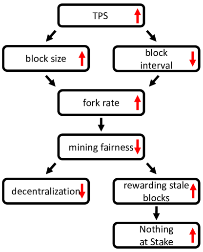
Mining fairness introduces a trade-off between the transaction processing capacity and decentralization in blockchain systems (Figure 1). We explain how increasing the system’s transaction processing capacity compromises decentralization. Transaction processing capacity depends on the number of transactions processed per block and the block generation interval. To increase this capacity, one might increase the block size and reduce the block generation interval. However, it is well-known that increasing block size and reducing block generation intervals result in a higher fork rate [2]. As previously observed, an increase in the fork rate undermines mining fairness. Reduced mining fairness means that some miner groups achieve higher profit rates than others. Consequently, miners with lower profit rates leave the system, while those with higher profit rates expand, leading to centralization and reduced decentralization.

The dilemma between transaction processing capacity and decentralization in blockchain systems arising from mining fairness has not yet been resolved. In this context, mining fairness is an inherent bottleneck for transaction processing capacity. Here, we demonstrate that the dilemma caused by mining fairness is inherent using the countermeasures adopted by Ethereum [3] (modified GHOST) as an example. Increasing the transaction processing capacity of the blockchain leads to more forks, which in turn causes two main issues. Firstly, there is an increased risk of attacks such as 51% attacks and Selfish Mining [4] [5]. Secondly, there is damage to mining fairness. Ethereum addressed the first issue by introducing GHOST. To address the latter issue of mining fairness, Ethereum partially rewards blocks that cause forks but are not incorporated into the main chain (stale blocks). However, this approach has its own problems. From another perspective, this means that even blocks that cause forks can receive block rewards, thereby reinforcing the economic incentives for attacks such as 51% attacks and Selfish Mining. This issue shares the same structure as the Nothing at Stake problem. In fact it is known that, in Ethereum, the risk of attacks that damage mining fairness, including Selfish Mining [4], increases [6] [7] [8]. This indicates that the measures taken by Ethereum do not fundamentally solve the issue of mining fairness.

From the above, analyzing mining fairness is a critical issue. Firstly, simulations are one possible method for this analysis. However, simulations are time-consuming and impractical. Consequently, alternative approaches have been explored[9, 10, 11, 12, 13, 14]. Nevertheless, existing methods do not correctly account for the damage to mining fairness caused by forks (6.1). As a result, analyses using these methods have a weak correlation with real-world systems, making meaningful discussions difficult.

In this study, we propose a model-based calculation method for quantitatively analyzing mining fairness. We approximate the blockchain network with a simplified model, assuming that each round contains at most two blocks. A round $r$ is defined as a unit of time that starts with the creation of a block at height $r$. Essentially, this means we assume that at most one fork occurs per round. This modeling approach simplifies the analysis of complex blockchain networks.

We validate the accuracy of the model-based calculation in measuring mining fairness through simulation experiments. Due to computational constraints, validation in large-scale networks is challenging. Therefore, we conduct validations in networks with a small number of miners. Our results demonstrate that the model-based calculation can measure mining fairness with high accuracy.

The model-based calculation enables efficient and comprehensive analysis of mining fairness. In this study, we analyze mining fairness using the model-based calculation. Initially, we examine mining fairness in a simple network composed of two miners. Subsequently, we investigate the impact of hashrate distribution on mining fairness. Finally, we reassess existing blockchain network improvement methods from the perspective of mining fairness.

2 Rounds

Figure 2: Rounds in the blockchain. The interval enclosed by the orange dotted line represents a single round in the blockchain.

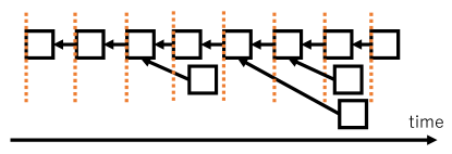
A round in a blockchain is a time interval defined from a global perspective. Specifically, round $r$ refers to the time from the first generation of a block at height $r$ until the first generation of a block at height $r+1$. The height of round $r$ is defined as $r$.

Since forks occur probabilistically within a blockchain network, the number of blocks per round is not always one. After the first block at height $r$ has been generated, another miner may generate a new block before the first block is propagated throughout the network. It should be noted that not all blocks generated in round $r$ have a height of $r$. For example, a miner unaware of the block at height $r-1$ will generate a block at height $r-1$ during round $r$ (Figure 2).

The round rate of each miner is defined as the probability that the miner initiates a round. Note that the round rate does not equal the proportion of the hashrate, due to forks.

With the introduction of rounds, we can formally define the fork rate. The fork rate is the probability that the number of blocks per round is two or more. When the number of blocks per round is two or more, the blockchain actually forks. Therefore, this definition includes the intuitive meaning of a fork.

3 Model-based calculation

3.1 Model

We approximate a complex blockchain network with a simplified model to calculate mining fairness. First, we define the set of miners as $V$, and let $N$ be the number of elements in $V$. The proportion of the hashrate of miner $i$ ($i\in V$) is denoted as $\alpha_{i}$. When a new block is generated within the network, the probability that miner $i$ generates that block is equal to the proportion of their hashrate, $\alpha_{i}$. The number of blocks generated in each round is assumed to be at most two, implying that there is at most one fork in each round.

Let $F_{ij}$ be the probability that miner $j$ generates a block that causes a fork within round $r$ started by miner $i$. After a fork occurs, as additional blocks are generated, one of the blocks will be incorporated into the main chain while the other will not. Let $W_{ij}$ be the probability that the block generated by miner $i$ is incorporated into the main chain when round $r$ starts with the block generated by miner $i$ and miner $j$ generates a block that causes the fork.

3.2 Definition of Mining Fairness

Before calculating mining fairness, we define mining fairness. In this study, mining fairness is divided into local mining fairness and global mining fairness. We define the following two measures as local mining fairness, $LF$:

$$LF_{1}(i) =r_{i}-\alpha_{i}$$ (1)

$$LF_{2}(i) =\frac{LF_{1}(i)}{\alpha_{i}}$$ (2)

Here, $r_{i}$ refers to the block reward rate of each miner. $LF_{1}$ represents the profit of each miner, while $LF_{2}$ represents the profit rate of each miner.

Next, we define global mining fairness, $GF$, using local mining fairness as follows:

$$GF_{1} =\sum_{i\in V}LF_{1}(i)\quad(LF_{1}(i)>0)$$ (3)

$$GF_{2} =\max_{i\in V}LF_{2}(i)-\min_{i\in V}LF_{2}(i)$$ (4)

$GF_{1}$ is the sum of $LF_{1}$ values that are positive. $GF_{2}$ represents the maximum difference in profit rates. Other mining fairness measures can also be defined using $LF$.

3.3 Calculation of Mining Fairness

This section demonstrates a computational method of mining fairness based on the above model. Firstly, we determine the round rate. Next, we calculate the local mining fairness $LF_{1}$, which is the difference between each miner’s block reward rate and the proportion of the hashrate. We also determine each miner’s profit rate $LF_{2}$. After calculating the local mining fairness, the global mining fairness can be easily calculated.

Let $X_{r}$ be the random variable representing the miner that generates the block starting round $r$. The following equation holds:

$$P(X_{r+1}=i)=\sum_{j\in V}\left(\alpha_{i}(1-F_{ji})+\sum_{k}\alpha_{k}F_{jk}\alpha_{i}\right)P(X_{r}=j)$$ (5)

Note that $P(X_{r+1}=i)$ depends only on $P(X_{r}=j)$. Therefore, the stochastic process ${X_{r}}{r=0}^{\infty}$ is a Markov chain. Additionally, since $F{ij}$ is less than 1 and $\alpha_{i}(1-F_{ji})+\sum_{k}\alpha_{k}F_{jk}\alpha_{i}$ is usually positive, this Markov chain is ergodic in most cases. Consequently, a unique stationary distribution exists, and the limiting distribution is the stationary distribution. we can determine the stationary distribution by iterating equation 5.

Let the limiting distribution be $\pi$. This represents the distribution of the miners generating blocks that start rounds after sufficient time has passed. Using $\pi$, the block reward rate $r_{i}$ for each miner is given by the following equation:

$$r_{i}= \pi(i)(1-\sum_{j\in V}\alpha_{j}F_{ij}+\sum_{j\in V}\alpha_{j}F_{ij}W_{ij})$$

$$+\sum_{j\in V}\pi(j)\alpha_{i}F_{ji}(1-W_{ji})$$ (6)

Thus, the $LF_{1}$ of miner $i$ is as follows:

$$LF_{1}(i)= r_{i}-\alpha_{i}$$ (7)

$$= \pi(i)(1-\sum_{j\in V}\alpha_{j}F_{ij}+\sum_{j\in V}\alpha_{j}F_{ij}W_{ij})$$

$$+\sum_{j\in V}\pi(j)\alpha_{i}F_{ji}(1-W_{ji})-\alpha_{i}$$ (8)

$LF_{2}$ can be calculated as follows:

$$LF_{2}(i)=\frac{LF_{1}(i)}{\alpha_{i}}$$ (9)

3.4 Algorithm

In this section, we describe the algorithm used in this paper to calculate mining fairness, as detailed in Section 3.3.

Algorithm 1 employs an iterative method to compute the mining fairness of each miner. The round rate calculation is performed between lines 9 and 27. Specifically, the fork rate is precomputed between lines 10 and 16. The variable loop manages the operations executed in each iteration. The calculations within the for loop from lines 20 to 26 follow the same process as described in Equation 5. Mining fairness is computed between lines 28 and 34, with the for loop calculations corresponding to Equations 8 and 9.

Algorithm 1 calculating the local mining fairness

1:the following variables are provided by the model.

2:$V$ $\triangleright$ the set of miners

3:$N$ $\triangleright$ the number of miners

4:$\alpha[N]$ $\triangleright$ the proportion of hashrate

5:$F[N][N]$ $\triangleright$ fork rate

6:$W[N][N]$ $\triangleright$ winning rate

7:

8:Our goal is to calculate the following values.

9:$\pi[N][2]$ $\triangleright$ round rate

10:$LF_{1}[N]$ $\triangleright$ $LF_{1}$

11:$LF_{2}[N]$ $\triangleright$ $LF_{2}$

12:

13:Calculating the round rate of each miner.

14:$\epsilon$ $\triangleright$ error

15:$dp[N]$ $\triangleright$ for dynamic programming

16:for $i\in V$ do

17:     $dp[i]\leftarrow 0$

18:     for $j\in V$ do

19:         $dp[i]\leftarrow\alpha_{j}F[i][j]$

20:     end for

21:end for

22:$loop\leftarrow 0$

23:while $\exists i\in Vs.t.|\pi[i][loop\ mod\ 2]-\pi[i][(loop+1)\ mod\ 2]|>\epsilon$ do

24:     $loop\leftarrow(loop+1)\ mod\ 2$

25:     for $i\in V$ do

26:         $\pi[i][(loop+1)\ mod\ 2]\leftarrow 0$

27:         for $j\in V$ do

28:              $\pi[i][(loop+1)\ mod\ 2]\leftarrow\pi[i][(loop+1)\ mod\ 2]+\alpha_{i}(1-F_{ji})\pi[j][loop]$

29:              $\pi[i][(loop+1)\ mod\ 2]\leftarrow\pi[i][(loop+1)\ mod\ 2]+dp[j]\alpha_{i}\pi[j][loop]$

30:         end for

31:     end for

32:end while

33:

34:Calculating the local fairness of each miner.

35:for $i\in V$ do

36:     $LF_{1}[i]\leftarrow\pi[i][(loop+1)\ mod\ 2]-\alpha[i]$

37:     for $j\in V$ do

38:         $LF_{1}[i]\leftarrow LF_{1}[i]+\pi(j)\alpha_{i}F_{ji}(1-W_{ji})-\pi(i)\alpha_{j}F_{ij}(1-W_{ij})$

39:     end for

40:     $LF_{2}[i]\leftarrow LF_{1}[i]/\alpha[i]$

41:end for

3.5 Parameters

3.5.1 How to determine $F_{ij}$

Let $T$ denote the average block generation interval, and let $T_{ij}$ represent the time it takes for a block generated by miner $i$ to be received by miner $j$. Then, $F_{ij}$ is defined as follows:

$$F_{ij} =\int_{0}^{T_{ij}}\frac{e^{-\frac{x}{T}}}{T}\,dx$$ (10)

$$=1-e^{-\frac{T_{ij}}{T}}$$ (11)

3.5.2 How to determine $W_{ij}$

Before explaining $W_{ij}$, it is essential to discuss chain conflicts.

Each miner constructs chains from their blocks and selects one main chain among them. The rule for selecting this chain is called the fork choice rule. In Bitcoin, the longest chain rule, which selects the longest chain, is adopted.

However, the fork choice rule alone may not uniquely determine the main chain due to forks. This situation is known as a chain tie. The rule to resolve chain ties is called the tie-breaking rule. In Bitcoin, the first-seen rule, which selects the chain learned about first, is adopted.

Practical tie-breaking rules can be broadly categorized as follows:

First-seen rule

This method selects the earliest arriving chain among the chains in a tie. It is adopted in Bitcoin.

Random rule

This method randomly selects a chain among the chains in a tie[4]. It was proposed as a countermeasure to Selfish Mining and was adopted in Ethereum.

Last-generated rule

This method selects the latest chain among the chains in a tie [15, 16]. It is a method that suppresses Selfish Mining more effectively than the random rule.

Next, we explain how to determine $W_{ij}$. $W_{ij}$ is significantly influenced by the hashrate of miners mining on the block generated by miner $i$ during a fork. Specifically, $W_{ij}$ is largely affected by the following two factors:

Tie-breaking rule

During a fork, chain ties often occur. The tie-breaking rule determines the block on which miners, other than the block generator, will mine.

Proportion of the hashrate of the block generator

The block generator mines on its own generated block regardless of the tie-breaking rule.

Other factors, such as block propagation time and the number of miners participating in the network, also influence $W_{ij}$. Refer to the validation section for details on the specific calculation methods of $W_{ij}$.

4 Validation

We validate that the model-based calculation can accurately compute mining fairness. First, we examine the assumption that the number of blocks per round is at most two from the perspective of the scale of the fork. Next, we compare the results of simulation experiments with those of the model-based calculations. Although calculating mining fairness through simulations of networks composed of many (around 100 or more) miners is excessively time-consuming, it is feasible to calculate mining fairness accurately and relatively quickly for networks with a small number of miners (2 to 10). In this study, we perform validation using networks consisting of 2 miners and 10 miners.

4.1 Considering the Scale of Forks

The model-based calculation disregards the impact of large-scale forks. Specifically, it assumes that the number of blocks per round is at most two. In this study, we investigate the effects of large-scale forks.

About the Scale of Forks First, we confirm some facts regarding fork rates. Let the hashrate of miner $i$, where $i\in V$, be $M_{i}$. Let the total network hashrate be $M_{all}$. Next, let $p$ be the probability of successfully generating a block with one hash calculation. In this case, the average number of hash calculations required to generate a block is $1/p$. Therefore, the following equation holds:

$$\frac{1}{pM_{all}}=T$$ (12)

where $T$ is the average block generation interval.

Next, let $N_{i}$ be the total number of hash calculations performed by miners who are unaware of the block generated by miner $i$. In this case, the following equation holds:

$$N_{i}=\sum_{j\in V}M_{j}T_{ij}$$ (13)

Next, let $T_{W,i}$ be the hashrate-weighted average block propagation time for the block generated by miner $i$. In this case, the following equation holds:

$$T_{W,i}=\sum_{j\in V}\alpha_{j}T_{ij}$$ (14)

Therefore, from equations 12, 13, and 14, the following equation holds:

$$pN_{i} =p\sum_{j\in V}M_{j}T_{ij}$$ (15)

$$=\sum_{j\in V}\frac{M_{j}}{M_{all}}\frac{T_{ij}}{T}$$ (16)

$$=\frac{T_{W,i}}{T}$$ (17)

Next, we examine the occurrence rate of forks by their scale. Let the random variable $C_{i}$ denote the number of blocks in the round initiated by miner $i$. In this case, the following holds:

$$P(C_{i}=1) =\sum_{j\in V}\alpha_{j}\int_{T_{ij}}^{\infty}e^{-\frac{x}{T}}dx$$ (18)

$$=\sum_{j\in V}\alpha_{j}e^{-\frac{T_{ij}}{T}}$$ (19)

$P(C_{i}=1)$ corresponds to the probability that no fork occurs. Next, the following holds:

$$P(C_{i}\neq 1) =1-P(C_{i}=1)$$ (20)

$$=1-\sum_{j\in V}\alpha_{j}e^{-\frac{T_{ij}}{T}}$$ (21)

$P(C_{i}\neq 1)$ corresponds to the probability that a fork occurs.

The probability that the number of blocks in a round will be 3 or more satisfies the following inequality:

$$P(C_{i}\geq 3) \leq\sum_{k=2}^{\infty}\binom{N_{i}}{k}p^{k}(1-p)^{N_{i}-k}$$ (22)

$$=\sum_{k=2}^{\infty}\frac{N_{i}\cdots(N_{i}-k+1)}{k!}p^{k}(1-p)^{N_{i}-k}$$ (23)

$$\leq\sum_{k=2}^{\infty}\frac{(pN_{i})^{k}}{k!}e^{-p(N_{i}-k)}$$ (24)

$$=e^{-pN_{i}}\sum_{k=2}^{\infty}\frac{(e^{p}pN_{i})^{k}}{k!}$$ (25)

$$=e^{-pN_{i}}(e^{e^{p}pN_{i}}-1-e^{p}pN_{i})$$ (26)

$$=e^{-\frac{T_{W,i}}{T}}(e^{e^{p}\frac{T_{W,i}}{T}}-1-e^{p}\frac{T_{W,i}}{T})$$ (27)

$$\xrightarrow[\frac{T_{W,i}}{T}\ \text{is constant}]{p\ \to\ 0}1-(1+\frac{T_{W,i}}{T})e^{-\frac{T_{W,i}}{T}}$$ (28)

When the number of blocks in a round is 3 or more, at least 3 hash calculations succeed before all the blocks are fully shared, thus satisfying inequality 22. Equation 27 is obtained by substituting equation 17 into equation 26.

From inequality 28, it follows that the probability that the number of blocks in a round will be 2 satisfies the following inequality:

$$P(C_{i}=2) =P(C_{i}\neq 1)-P(C_{i}\geq 3)$$ (29)

$$\geq\sum_{j\in V}\alpha_{j}(1-e^{-\frac{T_{ij}}{T}})-\left\{1-(1+\frac{T_{W,i}}{T})e^{-\frac{T_{W,i}}{T}}\right\}$$ (30)

$$=(1+\frac{T_{W,i}}{T})e^{-\frac{T_{W,i}}{T}}-\sum_{j\in V}\alpha_{j}e^{-\frac{T_{ij}}{T}}$$ (31)

Impact by Fork Scale We define the impact $I_{1}$ for rounds with one block, the impact $I_{2}$ for rounds with two blocks, and the impact $I_{3}$ for rounds with three or more blocks as follows:

$$I_{1} =e^{-\frac{d}{T}}$$ (32)

$$I_{2} =(1+\frac{d}{T})e^{-\frac{d}{T}}-\sum_{j\in V}\alpha_{j}e^{-\frac{d}{T}}$$ (33)

$$=\frac{d}{T}e^{-\frac{d}{T}}$$ (34)

$$I_{3} =1-(1+\frac{d}{T})e^{-\frac{d}{T}}$$ (35)

These definitions are obtained by substituting $T_{ij}=d$ into inequalities 19, 22, and 28. It should be noted that $I_{2}$ is defined based on the lower bound, and $I_{3}$ is defined based on the upper bound. In other words, $I_{2}$ is evaluated to be smaller, and $I_{3}$ is evaluated to be larger.

Figure 3: Comparison between $I_{3}$ and $I_{1}+I_{2}$

Figure 4: Comparison between $I_{3}$ and $I_{2}$

TABLE I: Influence of $I_{3}$ relative to $I_{1}$ and $I_{2}$.

	$d/T$
	0.01	0.1	0.5
$I_{3}/(I_{1}+I_{2})$	0.0000486868	0.00384871	0.0364743
$I_{3}/I_{2}$	0.0050167084	0.0517091	0.297442

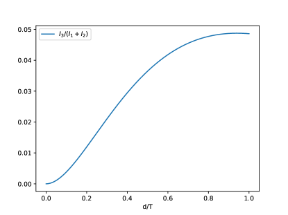
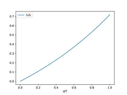
In the model-based calculation of mining fairness, we consider cases where the number of blocks per round is two or less, thereby ignoring $I_{3}$. Thus, we compare $I_{3}$ with $I_{1}$ and $I_{2}$. Figures 3 and 4 show $I_{3}/(I_{1}+I_{2})$ and $I_{3}/I_{2}$, respectively, as $d/T$ varies from $0$ to $1$. The specific numerical results are shown in Table I. From both the figures and the table, it is evident that as $d/T$ decreases, the influence of $I_{3}$ diminishes. While these figures and the table do not directly demonstrate that the model-based calculation can determine actual mining fairness, they suggest that the model-based calculation will be effective in scenarios where $d/T$ is small.

4.2 Network Composed of Two Miners

The comparison of the impact of forks by scale in Section 4.1 offers intuitive insight into how the assumption of the model affects the model-based calculation. However, it does not address how accurately the model-based calculation matches the actual numerical results of mining fairness. In this section, we validate the model-based calculation using a simple network composed of two miners.

4.2.1 Model-Based Calculation

We conduct the model-based calculation in a network composed of two miners. Following the procedure outlined in Section 3.3, we perform the calculations.

First, before the specific calculations, we provide some definitions. Let the two miners in the network be $Miner_{A}$ and $Miner_{B}$. Let the proportion of the hashrate of $Miner_{A}$ be $\alpha_{A}$ and that of $Miner_{B}$ be $\alpha_{B}$, where $\alpha_{A}+\alpha_{B}=1$. Let $T$ be the average block generation interval, and $d$ be the block propagation time. Let $\pi_{A}$ and $\pi_{B}$ be the round rates of $Miner_{A}$ and $Miner_{B}$, respectively. Next, we define $f$ as follows:

$$f =1-e^{-\frac{d}{T}}$$ (36)

This represents the probability that $Miner_{B}$ (or $Miner_{A}$) will create a fork when $Miner_{A}$ (or $Miner_{B}$) starts a round and the other miner generates the next block.

Next, we calculate the round rate. Considering that a sufficiently long time has passed, the following equation holds:

$$\pi_{B}=\pi_{A}(\alpha_{B}f\alpha_{B}+\alpha_{B}(1-f))+\pi_{B}(\alpha_{B}+\alpha_{A}f\alpha_{B})$$ (37)

$$\Rightarrow \pi_{B}(1-\alpha_{B}-\alpha_{A}f\alpha_{B})=\pi_{A}(\alpha_{B}f\alpha_{B}+\alpha_{B}(1-f))$$ (38)

$$\Rightarrow (1-\pi_{A})(1-\alpha_{B}-\alpha_{A}f\alpha_{B})=\pi_{A}(\alpha_{B}f\alpha_{B}+\alpha_{B}(1-f))$$ (39)

$$\Rightarrow \pi_{A}(f\alpha_{B}(\alpha_{B}-1-\alpha_{A})+1)=1-\alpha_{B}-\alpha_{A}f\alpha_{B}$$ (40)

$$\Rightarrow \pi_{A}(1-2\alpha_{A}\alpha_{B}f)=1-\alpha_{B}-\alpha_{A}f\alpha_{B}$$ (41)

$$\Rightarrow \pi_{A}=\alpha_{A}\frac{1-\alpha_{B}f}{1-2\alpha_{A}f\alpha_{B}}$$ (42)

Since $\pi_{A}$ has been calculated, $\pi_{B}$ can be determined as follows.

$$\pi_{B} =1-\pi_{A}$$ (43)

$$=\alpha_{B}\frac{1-\alpha_{A}f}{1-2\alpha_{A}f\alpha_{B}}$$ (44)

Next, we calculate the probability $W_{AB}$ that the block of $Miner_{A}$ is incorporated into the main chain when $Miner_{B}$ generates a block by forking immediately after $Miner_{A}$ starts a round. For simplicity, we assume that the block of $Miner_{B}$ conflicts with the chain of $Miner_{A}$. In other words, we ignore the case where the block height of $Miner_{B}$ is smaller than that of $Miner_{A}$.

$$W_{AB}= \overset{1}{\alpha_{A}}\overset{2}{\alpha_{A}}+\overset{1}{\alpha_{A}}\overset{2}{\alpha_{B}}(1-f)$$

$$+\overset{1}{\alpha_{A}}\overset{1}{\alpha_{B}}f\{\overset{2}{\alpha_{A}}\overset{3}{\alpha_{A}}+\overset{2}{\alpha_{A}}\overset{3}{\alpha_{B}}(1-f)$$

$$+\overset{2}{\alpha_{A}}\overset{2}{\alpha_{B}}f(\cdots)+\overset{2}{\alpha_{A}}\overset{2}{\alpha_{B}}f(\cdots)\}$$

$$+\overset{1}{\alpha_{A}}\overset{1}{\alpha_{B}}f\{\overset{2}{\alpha_{A}}\overset{3}{\alpha_{A}}+\overset{2}{\alpha_{A}}\overset{3}{\alpha_{B}}(1-f)$$

$$+\overset{2}{\alpha_{A}}\overset{2}{\alpha_{B}}f(\cdots)+\overset{2}{\alpha_{A}}\overset{2}{\alpha_{B}}f(\cdots)\}$$ (45)

$$= \alpha_{A}\alpha_{A}+\alpha_{A}\alpha_{B}(1-f)$$

$$+2\alpha_{A}\alpha_{B}f\{\alpha_{A}\alpha_{A}+\alpha_{A}\alpha_{B}(1-f)+2\alpha_{A}\alpha_{B}f(\cdots)\}$$ (46)

$$= \{\alpha_{A}\alpha_{A}+\alpha_{A}\alpha_{B}(1-f)\}\frac{1}{1-2\alpha_{A}\alpha_{B}f}$$ (47)

$$= \alpha_{A}\frac{1-\alpha_{B}f}{1-2\alpha_{A}\alpha_{B}f}$$ (48)

In equation 45, $\alpha_{A}$ and $\alpha_{B}$ represent the probabilities of $Miner_{A}$ and $Miner_{B}$ generating a block, respectively. The superscript numbers on $\alpha_{A}$ and $\alpha_{B}$ indicate the differences in block height from the block that initially caused the chain tie. The $W_{BA}$ can also be derived from $W_{AB}$ as follows:

$$W_{BA} =\alpha_{B}\frac{1-\alpha_{A}f}{1-2\alpha_{A}\alpha_{B}f}$$ (49)

Interestingly, the following relationships hold:

$$\pi_{A} =W_{AB}$$ (50)

$$\pi_{B} =W_{BA}$$ (51)

4.2.2 Simulation Settings

Based on the blockchain network simulator SimBlock [17], we developed an event-driven simulator composed of two miners. Our simulator is capable of simulating forks of any scale, similar to real blockchain systems.

We examined the ratios of block propagation time to average block generation interval, $d/T$, with values of $0.1$, $0.3$, and $0.5$. The block propagation time among all different miners was kept constant.

We also examined the proportion of hashrate of miner $A$, $\alpha_{A}$, with values of $0.1$ and $0.3$. The case of $0.5$ was not considered, as the mining fairness is completely maintained due to the network’s symmetry.

Each simulation consisted of 10 billion rounds.

TABLE II: Error between simulation values and the model-based calculations of $LF_{1}$.

		$d/T$
		0.1	0.3	0.5
$\alpha_{A}$	0.3	0.00059936	0.00792584	0.0203151
	0.1	0.000315594	0.0031603	0.00744887

4.2.3 Validation Results

The error between the simulation results and the model-based calculation results is shown in Table II. Here, the error is defined as the relative error as follows.

$$\frac{d(LF_{simulation},LF_{MBC})}{d(LF_{simulation,0})}$$ (52)

where $d$ is the Euclidean distance, $LF_{simulation}$ is the vector of simulated values of local mining fairness for each miner, and $LF_{MBC}$ is the vector of model-based calculated values of local mining fairness.

From the table, it can be seen that the model-based calculations can compute mining fairness with high accuracy. It can also be observed that the accuracy deteriorates as $d/T$ increases. This is likely because, as seen in 4.1, the influence of having more than three blocks per round becomes more significant as $d/T$ increases.

4.3 Network Composed of 10 Miners

In this section, we validate the model-based calculation of mining fairness in a network composed of 10 miners. Compared to a network with 2 miners, a network with 10 miners introduces additional elements such as tie-breaking rules, hashrate distribution, and block propagation time. This allows us to demonstrate that the model-based calculations function effectively even in more complex networks.

4.3.1 $W_{ij}$ in a Network Composed of Multiple Miners

In a network with more than two miners, it is necessary to consider tie-breaking rules. Here, we demonstrate how to determine $W_{ij}$ in a network with multiple miners according to different tie-breaking rules. It is assumed that all forks cause chain ties.

First-Seen Rule We assume that miner $i$ starts a round, and then miner $j$ causes a chain tie in the same round. Let $p_{i,j,k}$ be the probability that miner $k$ mines on the block generated by miner $i$. The time $T_{ij}$ it takes for the block generated by miner $i$ to reach miner $j$ is assumed to be a fixed value depending only on $i$ and $j$.

First, when $T_{ik}<T_{jk}$, regardless of the time when miner $j$ generated the block, the block generated by miner $i$ will reach miner $k$ first, hence $p_{i,j,k}=1$. Similarly, when $T_{ik}<T_{ij}+T_{jk}$, the block generated by miner $j$ will reach miner $k$ first, hence $p_{i,j,k}=0$. In other cases, the following equation holds:

$$p_{i,j,k} =\frac{\int_{T_{ik}-T_{jk}}^{T_{ij}}\frac{e^{-\frac{x}{T}}}{T}dx}{F_{ij}}$$ (53)

$$=\frac{e^{-\frac{T_{ik}-T_{jk}}{T}}-e^{-\frac{T_{ij}}{T}}}{1-e^{-\frac{T_{ij}}{T}}}$$ (54)

Equation 53 represents the probability that the block of miner $i$ reaches miner $k$ first under the condition that a chain tie occurs. Equation 54 substitutes $F_{ij}$ in equation 53 with equation 11.

From $p_{i,j,k}$, $W_{ij}$ is determined as follows:

$$W_{ij} =\sum_{k\in V}\alpha_{k}p_{i,j,k}$$ (55)

Random Rule In the random rule, mining is performed by selecting a block randomly during chain ties. The value $W_{ij}$ is given by the following equation:

$$W_{ij} =\alpha_{i}+\frac{1-\alpha_{i}-\alpha_{j}}{2}$$ (56)

Last-Generated Rule In the last-generated rule, mining is performed by selecting the most recently generated block during chain ties. The value $W_{ij}$ is given by the following equation:

$$W_{ij} =\alpha_{i}$$ (57)

Figure 5: The hashrate distribution used in the validation of the model-based calculation.

4.3.2 Simulation Settings

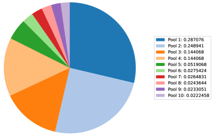
The simulator used in this validation is an extended version of a network simulator composed of two miners. The number of miners was set to 10. The hashrate distribution settings are shown in Table 5. The hashrate distribution is based on Bitcoin [18].

The ratios of the average block propagation time to the average block generation interval, $d/T$, examined in this validation are $0.01$, $0.04$, $0.07$ and $0.1$ [5, 19]. The block propagation time distribution among different miners follows an exponential distribution [2], while the block propagation time to oneself is set to 0. Additionally, the tie-breaking rules examined are the first-seen rule, random rule, and last-generated rule.

Each simulation consisted of 10 billion rounds.

TABLE III: Mean and standard deviation (SD) of error between simulation values and the model-based calculations for $d/T=0.01$ and $0.04$.

		first-seen rule		random rule		last-generated rule
		d/T
		0.01	0.04	0.01	0.04	0.01	0.04
round rate	mean	0.0000201254	0.000132747	0.0000208543	0.000134614	0.0000207662	0.000135
	SD	0.00000639285	0.0000648318	0.00000663684	0.0000664632	0.00000700959	0.0000649111
$LF_{1}$	mean	0.00891706	0.0221225	0.0153555	0.0507862	0.0214307	0.080677
	SD	0.00356624	0.0115312	0.00771275	0.0289467	0.0130309	0.0613974
$LF_{2}$	mean	0.0108707	0.0209106	0.0164265	0.0439469	0.0210495	0.0702858
	SD	0.00373994	0.00828696	0.00546804	0.0146293	0.0110262	0.0426435

TABLE IV: Mean and standard deviation (SD) of error between simulation values and the model-based calculations for $d/T=0.07$ and $0.1$.

		first-seen rule		random rule		last-generated rule
		d/T
		0.07	0.1	0.07	0.1	0.07	0.1
round rate	mean	0.000406944	0.0008385	0.0004072	0.000840025	0.000408239	0.000839217
	SD	0.000215053	0.000462696	0.000215627	0.000461556	0.000217068	0.000460759
$LF_{1}$	mean	0.0851189	0.0553571	0.0851189	0.117411	0.13679	0.188992
	SD	0.0467998	0.0293375	0.0467998	0.0630781	0.104206	0.141844
$LF_{2}$	mean	0.0737303	0.0520755,	0.0737303	0.10182	0.117051	0.159697
	SD	0.0242187	0.0205341	0.0242187	0.0328015	0.0670573	0.0871817

4.3.3 Validation Results

We conducted 50 simulation experiments for each validation target. The errors between the simulation results and the model-based calculations are shown in Tables III and IV. Here, the error is defined as the relative error previously defined. The difference from the previous validation is that the number of elements in the $LF$ vector has changed from 2 to 10 and we investigate not only the $LF$ vector but also the round rate vector.

First, we examine the round rate. It can be seen that the model-based calculations match the simulation results with high accuracy under all conditions.

Next, we look at mining fairness. From the tables, it can be seen that the model-based calculations are able to compute mining fairness with high accuracy. It can also be observed that the accuracy deteriorates as $d/T$ increases.

It is also found that the accuracy of mining fairness calculations is not as high as that of round rate calculations or mining fairness calculations in a network composed of two miners. This is because the mining fairness calculation requires $W_{ij}$.

Additionally, it is observed that the first-seen rule is more accurate than the random rule or the last-generated rule. This indicates that the calculation of $W_{ij}$ for the first-seen rule is superior. The reason for this is that the influence of the blocks up to the second one in the round is stronger in the first-seen rule.

5 Analysis

In this section, we conduct a detailed analysis of mining fairness using the model-based calculation. First, we analyze mining fairness in a simple network composed of two miners (Section 5.1). Next, we examine the impact of hashrate distribution on mining fairness (Section 5.2). Finally, we reassess existing blockchain network improvement methods from the perspective of mining fairness (Section 5.3).

5.1 Network Composed of Two Miners

In this section, we provide a thorough examination of mining fairness in a simple network that includes only two miners. Analyzing such a network offers two advantages: there is no need to consider tie-breaking rules, and it allows for a more general analysis without substituting specific values for the parameters. We investigate the properties of mining fairness using the model-based calculation in this network.

5.1.1 Analysis Subject

We analyze a network composed of two miners ($Miner_{A}$ and $Miner_{B}$). The block propagation time $d$ is fixed between all different miners. The block propagation time to itself is assumed to be 0.

5.1.2 Analysis Results

We conducted an analysis based on the model-based calculation using $W_{ij}$ (See Section 4.2), which was validated in a network composed of two miners.

Figure 6: $LF_{1}(A)$ in a network composed of two miners.

TABLE V: $LF_{1}$ when varying $d/T$ and $\alpha_{A}$

		$d/T$
		0.1	0.2	0.3	0.4	0.5
$\alpha_{A}$	0.5	0	0	0	0	0
	0.7	0.0161907	0.0312103	0.045127	0.0580053	0.0699067
	0.9	0.0133946	0.0249514	0.034909	0.0434791	0.0508486

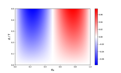
First, let’s examine the local mining fairness $LF_{1}(A)$ of $Miner_{A}$. Table V and Figure 6 illustrate $LF_{1}(A)$ with varying ratios of block propagation time to average block generation interval, $d/T$, and the proportion of hashrate of $Miner_{A}$, $\alpha_{A}$. From the figure, it is evident that as $d/T$ increases, mining fairness deteriorates.

TABLE VI: Maximum value of $LF_{1}$ and $\alpha_{A}$ at which the maximum value is achieved when $d/T$ is varied.

	$d/T$
	0.1	0.2	0.3	0.4	0.5
$LF_{1}$	0.0183165	0.0349033	0.0499354	0.0635683	0.0759402
$\alpha_{A}$	0.783959	0.779441	0.775129	0.771029	0.767144

Next, we focus on $\alpha_{A}$. By considering symmetry, we examine $\alpha_{A}$ from 0.5 to 1. When $\alpha_{A}$ is varied from 0.5 to 1, $LF_{1}$ is concave upwards. This can be attributed to the fact that as $\alpha_{A}$ increases, the power of $Miner_{A}$ to take rewards from $Miner_{B}$, but the number of blocks generated by $Miner_{B}$ decreases accordingly.

Therefore, we investigate the maximum value of $LF_{1}$ and the corresponding $\alpha_{A}$ when varying $d/T$ using ternary search. Table VI shows the results. As shown in the table, as $d/T$ increases, the maximum value of $LF_{1}$ increases, while the $\alpha_{A}$ at which this maximum value is achieved decreases.

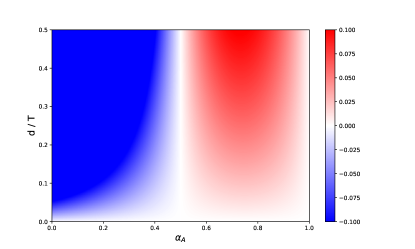
Next, we examine the local mining fairness of $Miner_{A}$, $LF_{2}(A)$. Table VII and Figure 7 show $LF_{2}(A)$ when $d/T$ and $\alpha_{A}$ are varied. From the table and figure, it is evident that as $d/T$ increases, mining fairness deteriorates.

Next, we focus on $\alpha_{A}$. Unlike $LF_{1}$, $LF_{2}$ does not exhibit symmetry. When $\alpha_{A}$ is varied from 0.0 to 0.5, $LF_{2}$ increases monotonically. When $\alpha_{A}$ is varied from 0.5 to 1, $LF_{2}$ is concave upwards. Therefore, we investigate the maximum value of $LF_{2}$ and the corresponding $\alpha_{A}$ when varying $d/T$ using ternary search. Table VIII shows the results. As shown in the table, as $d/T$ increases, the maximum value of $LF_{2}$ increases, while the $\alpha_{A}$ at which this maximum value is achieved decreases. It is also observed that the $\alpha_{A}$ at which the maximum value of $LF_{2}$ is achieved is slightly smaller than that for $LF_{1}$.

Figure 7: $LF_{2}(A)$ in a network composed of two miners.

TABLE VII: $LF_{2}$ when varying $d/T$ and $\alpha_{A}$.

		$d/T$
		0.1	0.2	0.3	0.4	0.5
$\alpha_{A}$	0.1	-0.00133946	-0.00249514	-0.0034909	-0.00434791	-0.00508486
	0.3	-0.00053969	-0.00104034	-0.00150423	-0.00193351	-0.00233022
	0.5	0	0	0	0	0
	0.7	0.000231296	0.000445862	0.000644671	0.000828646	0.000998668
	0.9	0.000148828	0.000277238	0.000277238	0.000483101	0.000564984

TABLE VIII: Maximum value of $LF_{2}$ and $\alpha_{A}$ at which the maximum value is achieved when $d/T$ is varied.

	$d/T$
	0.1	0.2	0.3	0.4	0.5
$LF_{1}$	0.0239401	0.0458883	0.0660208	0.0844949	0.101452
$\alpha_{A}$	0.74543	0.741098	0.737005	0.73315	0.729529

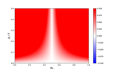
Next, we examine the global mining fairness. In a network composed of two miners, the property of $GF_{1}$ can be understood from $LF_{1}$. Therefore, we focus only on $GF_{2}$. Table IX and Figure 8 show $GF_{2}$ when varying $d/T$ and $\alpha_{A}$. It can be observed from the figure that as $d/T$ increases, mining fairness deteriorates. Next, we focus on $\alpha_{A}$. Due to symmetry, we consider the case where $\alpha_{A}$ is between 0.5 and 1. It can be seen that $GF_{2}$ increases monotonically as $\alpha_{A}$ increases.

Figure 8: $GF_{2}(A)$ in a network composed of two miners.

TABLE IX: $GF_{2}$ when varying $d/T$ and $\alpha_{A}$.

		$d/T$
		0.1	0.2	0.3	0.4	0.5
$\alpha_{A}$	0.5	0	0	0	0	0
	0.7	0.0542003	0.10448	0.151068	0.194179	0.234021
	0.9	0.134094	0.249791	0.349478	0.435274	0.509051

5.2 Impact of Hashrate Distribution

In this section, we explore how the hashrate distribution affects mining fairness. Different hashrate distributions can lead to varying degrees of mining fairness. we aim to identify patterns by analyzing these distributions.

5.2.1 Analysis Subjects

Block Propagation Time and Average Block Generation Interval We analyze the ratios of propagation time to average block generation interval, $d/T$, of 0.01, 0.04, and 0.07. The block propagation time is fixed among all different miners, and the propagation time to oneself is set to 0.

Tie-breaking Rule We analyze three tie-breaking rules: the first-seen rule, the random rule, and the last-generated rule.

(a) Bitcoin

(b) Dogecoin

(c) Bitcoin Cash

(d) Litecoin

(e) Ethereurm Classic

(f) Bitcoin SV

Figure 9: The hashrate distributions.

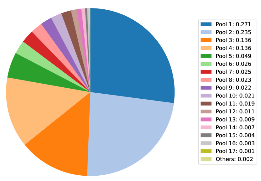
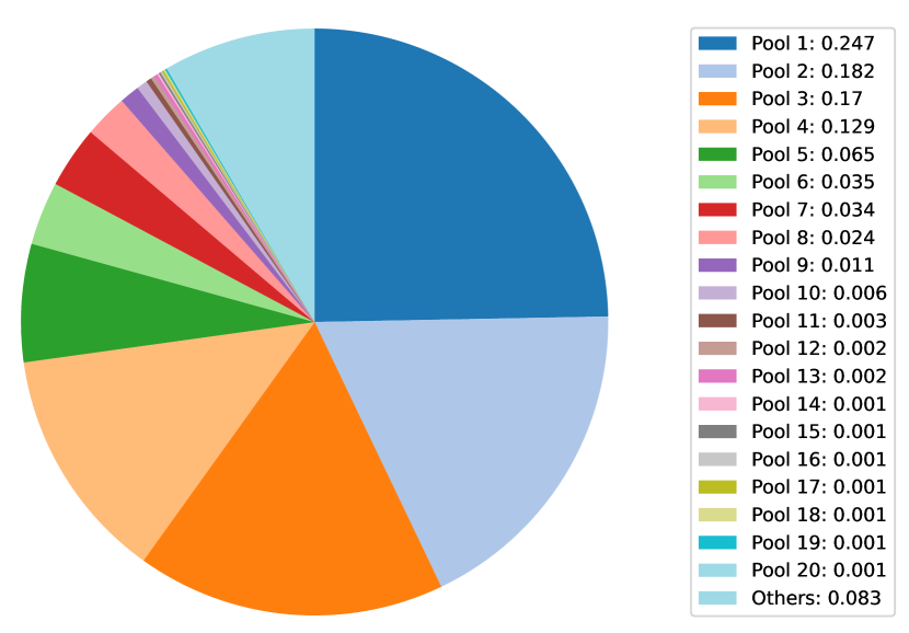
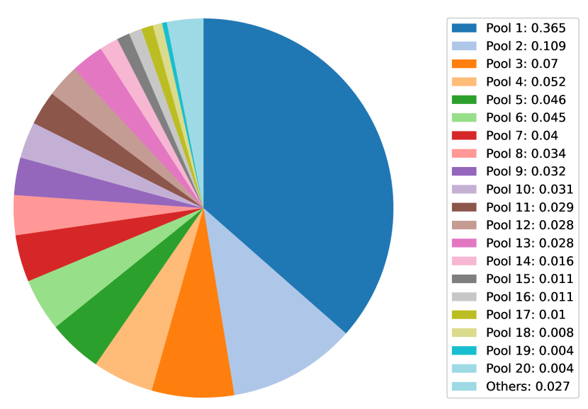
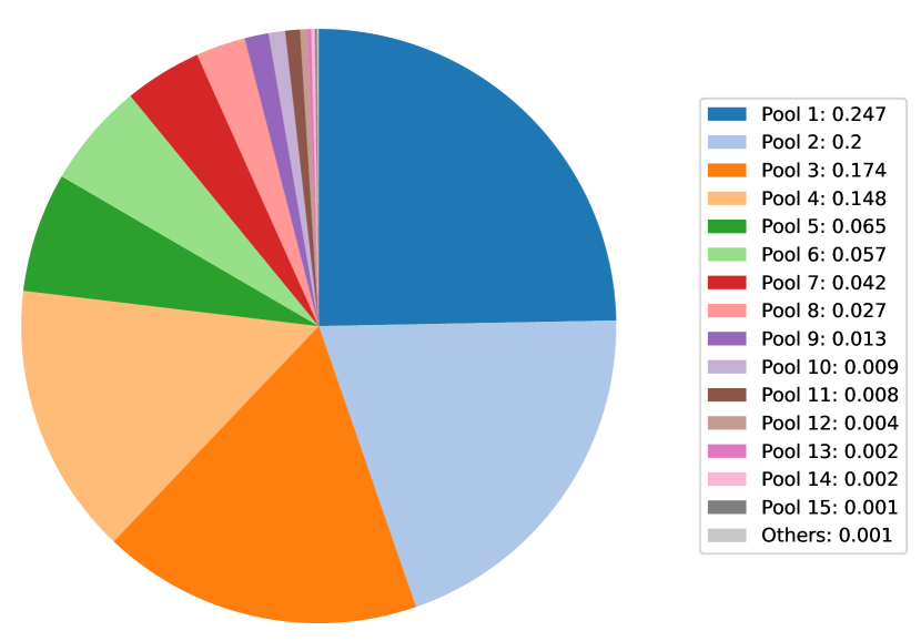
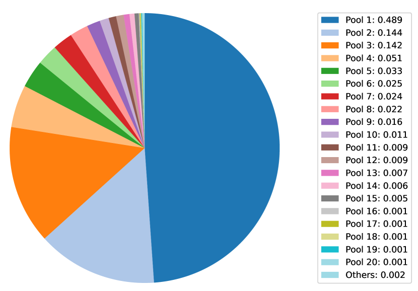
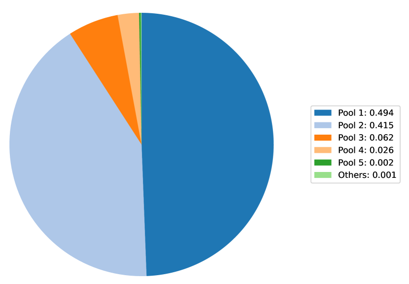
Hashrate Distribution and Number of Miners The number of miners is set to 100. We analyze six distributions of the hashrate ratio as shown in Figure 9 [18]. Specifically, we first allocate the hashrate ratios of Pools other than Others to miners. Then, the remaining hashrate ratio is evenly distributed among the remaining miners, ensuring that the total hashrate ratio of these miners equals the hashrate ratio of Others. Others corresponds to the total hashrate ratio of solo miners.

Figure 10: $LF_{2}$ with the hashrate distribution of Bitcoin and the first-seen rule.

5.2.2 Analysis Results

We conducted an analysis based on the model-based calculation using $W_{ij}$ in a network composed of 10 miners (see Section 4.3).

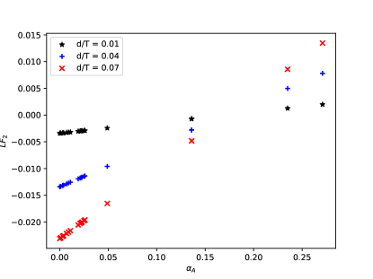
First, we confirmed that $LF_{2}$ becomes a linear function of $\alpha$. Figure 10 are scatter plots of $LF_{2}$ with the hashrate distribution of Bitcoin and the first-seen rule. From the figure, it is evident that $(\alpha,LF_{2})$ lies on a straight line regardless of the conditions. This fact is also true for any analysis subjects by the correlation coefficient, which averages 0.999995 with a standard deviation of 0.00000667953. Next, using the least squares method, we determined the slope of each line. Table X shows the results. Additionally, Table XI presents the mean, standard deviation, and coefficient of variation of the slopes for each column. From Table XI, it can be seen that the hashrate distribution has little effect on the slopes. Therefore, we assume that the slope is constant regardless of the hashrate distribution.

Next, we confirm the correlation between the slope of $LF_{2}$ and $d/T$. First, from equation 21 and fixing $d/T$, we derive the following approximate formula for the fork rate:

$$P(C_{i}\neq 1) =\sum_{j\in V}\alpha_{j}(1-e^{-\frac{T_{ij}}{T}})$$ (58)

$$=\sum_{j\in V}\alpha_{j}(1-e^{-\frac{d}{T}})$$ (59)

$$=(1-e^{-\frac{d}{T}})$$ (60)

Next, we compare the ratio of fork rates and the ratio of the slopes of $LF_{2}$ when $d/T$ is $0.01$ and $0.04$, as well as when $d/T$ is $0.01$ and $0.07$. Table XII shows the results. From the table, it is clear that the fork rate and the slope of $LF_{2}$ have a proportional relationship. As the fork rate increases with increasing $d/T$, it can be seen that the slope of $LF_{2}$ also increases with increasing $d/T$. This indicates that mining fairness is increasingly damaged as $d/T$ rises.

TABLE X: Comparison of slopes of $LF_{2}$

	first-seen rule			random rule			last-generated rule			$\Sigma_{i\in V}\alpha_{i}^{2}$
	$d/T$
	0.01	0.04	0.07	0.01	0.04	0.07	0.01	0.04	0.07
Bitcoin	0.0198907	0.0782723	0.134769	0.0198534	0.0776913	0.133039	0.019816	0.0771103	0.131308	0.171452
Dogecoin	0.0198916	0.0782865	0.134811	0.0198523	0.0776752	0.132992	0.0198131	0.0770643	0.131172	0.147123
Bitcoin Cash	0.0199034	0.0784709	0.135362	0.0198718	0.0779764	0.133884	0.0198401	0.0774819	0.132406	0.164704
Litecoin	0.0198894	0.0782515	0.134708	0.0198506	0.0776484	0.132912	0.0198118	0.0770452	0.131116	0.163495
Ethereum Classic	0.019889	0.0782462	0.134692	0.0198622	0.0778276	0.133442	0.0198353	0.077409	0.132192	0.28605
Bitcoin SV	0.0198645	0.0778646	0.133555	0.0198388	0.0774643	0.132364	0.019813	0.0770641	0.131172	0.420785

TABLE XI: Mean, standard deviation (SD), and coefficient of variation (CV) of slopes

	first-seen rule			random rule			last-generated rule
	$d/T$
	0.01	0.04	0.07	0.01	0.04	0.07	0.01	0.04	0.07
mean	0.0198881	0.078232	0.134649	0.0198548	0.0777138	0.133105	0.0198215	0.0771958	0.131561
SD	0.000011638	0.000181306	0.000540243	0.00001021106	0.000158341	0.000469727	0.0000115562	0.000178855	0.000528655
CV	0.000585178	0.00231754	0.00401221	0.000514285	0.00203749	0.00352898	0.000583015	0.0023169	0.00401833

TABLE XII: Comparison of fork rate and $LF_{2}$.

	fork rate	first-seen rule	random rule	last-generated rule
($d/T$ = 0.04) / ($d/T$ = 0.01)	3.94069	3.9336	3.91409	3.89453
($d/T$ = 0.07) / ($d/T$ = 0.01)	6.79447	6.77035	6.70392	6.63727

Next, we examine the root $\alpha_{0}$ of $LF_{2}$. First, since $LF_{2}$ can be expressed as a linear function of the proportion of hashrate $\alpha$, the following equation holds:

$$LF_{2}(i) =k(\alpha_{i}-\alpha_{0})$$ (61)

where $k$ is a constant determined by the tie-breaking rule and $d/T$.

From equation 61, $LF_{1}$ is derived as follows:

$$LF_{2}(i)\alpha_{i} =\alpha_{i}k(\alpha_{i}-\alpha_{0})$$ (62)

$$\iff LF_{1}(i) =k\alpha_{i}^{2}-k\alpha_{0}\alpha_{i}$$ (63)

By summing $LF_{1}$, we obtain:

$$\sum_{i\in V}LF_{1}(i) =\sum_{i\in V}\left(k\alpha_{i}^{2}-k\alpha_{0}\alpha_{i}\right)$$ (64)

$$\iff 0 =k\sum_{i\in V}\alpha_{i}^{2}-k\alpha_{0}\sum_{i\in V}\alpha_{i}$$ (65)

$$\iff\alpha_{0} =\sum_{i\in V}\alpha_{i}^{2}$$ (66)

Thus, $\alpha_{0}$ is equal to $\sum_{i\in V}\alpha_{i}^{2}$. It is evident from the following equation that $\sum_{i\in V}\alpha_{i}^{2}$ is related to the variance of the proportion of hashrate:

$$\sum_{i\in V}\alpha_{i}^{2} =N\left(\text{Var}[\alpha]+\frac{1}{N^{2}}\right)$$ (67)

Therefore, considering $N$ as fixed at 100, as the variance increases, $\sum_{i\in V}\alpha_{i}^{2}$ also increases, which in turn increases the root of $LF_{2}$. This implies that achieving a high profit rate becomes more difficult.

TABLE XIII: $GF_{1}$ and $GF_{2}$ for $d/T=0.01$.

	first-seen rule		random rule		last-generated rule		Variance
	$GF_{1}$	$GF_{2}$	$GF_{1}$	$GF_{2}$	$GF_{1}$	$GF_{2}$
Bitcoin	0.000833972	0.00539058	0.000832568	0.0053808	0.000831165	0.00537101	0.00161452
Dogecoin	0.000694512	0.00489436	0.000693225	0.00488519	0.000691937	0.00487602	0.00137123
Bitcoin Cash	0.00145547	0.00725821	0.00145333	0.00724673	0.0014512	0.00723525	0.00154704
Litecoin	0.000591993	0.00491319	0.000590934	0.00490398	0.000589874	0.00489477	0.00153495
Ethereum Classic	0.00197496	0.00972674	0.00197285	0.00971435	0.00197075	0.00970196	0.0027605
Bitcoin SV	0.000719277	0.00981355	0.000718751	0.00980117	0.000718225	0.00978879	0.00410785

Figure 11: $GF_{1}$ for various hashrate distribtutions.

Figure 12: $GF_{2}$ for various hashrate distribtutions.

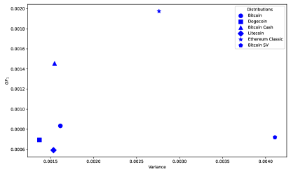
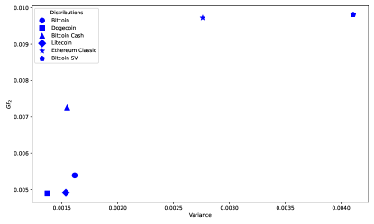
Next, we examine the relationship between variance and the global mining fairness in detail. We consider only the case where $d/T=0.01$. This is because, from the analysis of the slope of $LF_{2}$ and $d/T$ mentioned earlier, if the result for $d/T=0.01$ is understood, the results for $d/T=0.04$ and $0.07$ can also be inferred. Table XIII and Figures 11 and 12 show the global mining fairness when the hashrate distribution is changed. From the figures, it can be seen that $GF_{2}$ increases as the variance increases. A similar trend is observed for $GF_{1}$. However, in the case of Bitcoin SV, where the variance is extremely large, $GF_{1}$ takes a small value. This is because the root of $LF_{2}$ increases, resulting in a decrease in the profitability of miners with a large share of the hashrate.

5.3 Reassessing Existing Blockchain Network Improvement Methods

Despite the significance of analyzing mining fairness, existing methods for improving blockchain networks have not been evaluated from the perspective of mining fairness. Other metrics such as fork rate, stale rate, X%ile block propagation time, communication overhead, and average propagation time cannot substitute for mining fairness. For instance, even if the overall stale rate is high, mining fairness is achieved if all miners have an equal stale rate.

In this section, we re-evaluate existing methods for improving blockchain networks from the perspective of mining fairness. We also examine the relationship between block propagation time and mining fairness. Furthermore, we analyze the partial application of methods to improve blockchain networks.

We used SimBlock, a blockchain network simulator [17], to determine the block propagation time of each method. In SimBlock, miners had attributes such as region, hashrate, and neighbor nodes. There were a total of six regions. Bandwidth and latency are determined between regions. The hashrate distribution follows a normal distribution with a mean of $4\cdot 10^{8}$ (/sec) and a standard deviation of $1\cdot 10^{8}$ (/sec). Each miner had 8 outbound connections and up to 125 inbound connections. The number of miners was set to 1000, and the average block generation interval, $T$, was set to 600 seconds.

The analysis subjects are as follows:

Year 2019

SimBlock allows the setting of regional bandwidths and latencies for 2019, which we used [20]. Neighbor nodes were chosen randomly.

Year 2015

SimBlock allows the setting of regional bandwidths and latencies for 2015, which we used. Other conditions are the same as those in 2019.

Matsuura Method

The Matsuura method [21] was used for neighbor node selection. Specifically, out of 8 outbound connections, 6 were neighbor nodes within the region, and the number of inbound connections from outside the region was kept below 2. Other conditions are the same as those in 2019.

Aoki Method

An improved version of the Aoki method [22] was used for neighbor node selection. The specific improvements are as follows. The original Aoki method evaluated each neighbor node based on the time the INV message arrived. However, this method overestimates latency because the INV message size is very small, and the bandwidth impact on propagation time is minimal. In this study, each neighbor node was evaluated based on the time the block was received. This allows scoring that considers factors such as bandwidth and the number of neighboring miners besides latency. The number of neighbor nodes selected by this method, K, was set to 5, and the weight parameter, P, was set to 0.3. Other conditions are the same as those in 2019.

Compact Block Relay

The Compact Block Relay [23] was applied. SimBlock allows the setting of low-bandwidth Compact Block Relay, which we used [20].

Relay Network

A relay network was applied. The implementation was referenced from the paper by Otsuki et al. [24]. Specifically, relay servers were newly installed in each region. Communication between relay servers had their bandwidth reduced to 1/10. Additionally, relay servers propagated blocks in parallel to relay clients within the same region. Relay clients sent blocks to relay servers when they received them.

The calculation of mining fairness also takes into account tie-breaking rules. As in the previous analysis, we analyze the first-seen rule, random rule, and last-generated rule.

Figure 13: Combining blockchain network simulations and the model-based calculation.

The analysis was conducted by combining blockchain network simulations and the model-based calculations. First, we simulated the blockchain network improvement methods. Next, from these simulations, we obtained the proportion of hashrate of each miner and the block propagation time. Using the simulation results, we performed the model-based calculations to determine mining fairness (Figure 13).

To determine the block propagation time between miners, each miner generated and propagated blocks 10 times, and the average propagation time was calculated. In the case of Aoki Method, we simulated the blockchain for 10,000 blocks beforehand and then measured after changing the network topology.

Using the results obtained from the simulatons and the calculated $W_{ij}$ for a network consisting of 10 miners (see Section 4.3), we performed the model-based calculations.

In addition to the mining fairness calculation, we also calculated the hashrate-weighted average block propagation time $T_{W}$. $T_{W}$ is defined as follows:

$$T_{W}=\sum_{i\in V}\pi(i)T_{W,i}$$ (68)

Furthermore, from equation 21, the following equation holds:

$$\sum_{i\in V}\pi(i)P(C_{i}\neq 1) =\sum_{i\in V}\pi(i)\sum_{j\in V}\alpha_{j}(1-e^{-\frac{T_{ij}}{T}})$$ (69)

$$\approx\sum_{i\in V}\pi(i)\sum_{j\in V}\alpha_{j}\frac{T_{ij}}{T}$$ (70)

$$=\sum_{i\in V}\pi(i)\frac{T_{W,i}}{T}$$ (71)

$$=\frac{T_{W}}{T}$$ (72)

In other words, if $T_{ij}/T$ is sufficiently small, then $T_{W}$ is proportional to the fork rate. Therefore, by comparing $T_{W}$ and mining fairness, we can simultaneously analyze block propagation time, fork rate, and mining fairness.

TABLE XIV: Mining fairness for various methods.

	first-seen rule		random rule		last-generated rule		$T_{W}$(ms)
	$GF_{1}$	$GF_{2}$	$GF_{1}$	$GF_{2}$	$GF_{1}$	$GF_{2}$
Year 2019	0.00474988	0.0515219	0.00230566	0.0251254	0.00271252	0.0339676	2810.48
Year 2015	0.0176043	0.14418	0.00819617	0.0662684	0.0121374	0.0809427	7590.74
Matsuura method	0.00497753	0.0701467	0.00239605	0.0335915	0.00330603	0.0391697	2830.65
Aoki method	0.00306039	0.0442852	0.00151897	0.022104	0.00218897	0.0346884	1443.49
Compact Block Relay	0.00270534	0.0257198	0.00134564	0.012765	0.00139523	0.0119549	697.064
Relay Network	0.0047608	0.069336	0.0025588	0.0386536	0.00379238	0.054596	1377.98

Figure 14: $GF_{1}$ and $T_{W}$ for various methods.

Figure 15: $GF_{2}$ and $T_{W}$ for various methods.

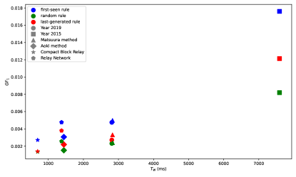
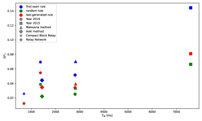
The experimental results are shown in Figures 14 and 15, and Table XIV. The correlation coefficients between $T_{W}$ and mining fairness are presented in Table XV. Table XIV shows the mining fairness for each method. Next, we focus on the relationship between $T_{W}$ and mining fairness. From Figures 14, 15, and Table XV, it is evident that there is a strong correlation between $T_{W}$ and mining fairness. However, when comparing Aoki Method and Relay Network, it is also clear that a smaller $T_{W}$ does not necessarily lead to an improvement in mining fairness. This highlights the significance of using mining fairness as an evaluation criterion, in addition to block propagation time and fork rate.

TABLE XV: Correlation coefficients between $T_{W}$ and mining fairness.

	first-seen rule	random rule	last-generated rule
$GF_{1}$	0.972241	0.965767	0.955618
$GF_{2}$	0.943214	0.897603	0.831644

Next, we analyze mining fairness in partial application. We investigate the difference in benefits between miners using the methods and those who do not. The analysis subjects are Matsuura Method, Aoki Method, Compact Block Relay, and Relay Network. Before the analysis, we define partial mining fairness ($PF$) as follows:

$$PF_{1}(W) =\sum_{i\in W}LF_{1}(i)\quad(W\subseteq V)$$ (73)

$$PF_{2}(W) =\max_{i\in W}LF_{2}(i)-\min_{i\in W}LF_{2}(i)$$ (74)

$PF_{1}$ indicates how much benefit the group of miners $W$ gains relative to the whole. $PF_{2}$ indicates the disparity of profit rates within the group of miners.

TABLE XVI: Mining fairness in partial application.

		first-seen rule		random rule		last-generated rule
		$PF_{1}$	$PF_{2}$	$PF_{1}$	$PF_{2}$	$PF_{1}$	$PF_{2}$
Matsuura method	$V^{+}$	0.000324868	0.0642711	0.000157235	0.0309625	-0.000037282	0.0454161
	$V^{-}$	-0.000324868	0.0634175	-0.000157235	0.0305188	0.000037282	0.0448585
Aoki method	$V^{+}$	0.0000664748	0.0464631	0.0000336752	0.0232355	-0.00000239572	0.0388238
	$V^{-}$	-0.0000664748	0.0451997	-0.0000336752	0.022562	0.00000239572	0.036586
Compact Block Relay	$V^{+}$	0.00119788	0.0545818	0.00059376	0.0272231	0.000991298	0.0381354
	$V^{-}$	-0.00119788	0.055761	-0.00059376	0.0276239	-0.000991298	0.0429945
Relay Network	$V^{+}$	0.00537498	0.0654808	0.002722	0.0342245	0.00495924	0.0477043
	$V^{-}$	-0.00537498	0.0662333	-0.002722	0.0330528	-0.00495924	0.0476327

Figure 16: $PF_{1}$ for various methods for various methods.

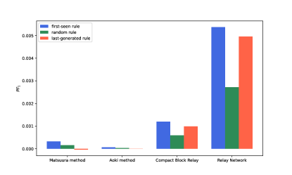
We divided the miners into two equal groups: one using a method and the other not. Let $V^{+}$ be the set of miners using a method, and $V^{-}$ be the set of miners not using the method. Table XVI and Figure 16 show the mining fairness in partial application. First, we focus on $PF_{1}$. It can be observed that there is almost no difference in $PF_{1}$ between $V^{+}$ and $V^{-}$ for both Matsuura Method and Aoki Method. This indicates that the neighbor node selection does not create a difference in $PF_{1}$ between miners using the method and those not using it. Next, it can be seen that miners using Relay Network benefit more than those using Compact Block Relay. This is believed to be due to the relay server propagating blocks faster only when the relay client generates a block. Additionally, focusing on $PF_{2}$, it is evident that there is no significant difference in the disparity within miners using the method and those not using it for all methods.

6 Discussion

6.1 Existing Analyses of Mining Fairness

Mining Fairness by Unintentional Forks Croman et al. proposed several metrics and solutions to address the scalability issues of blockchains [9]. They highlighted mining fairness as a potentially more valuable metric, despite its difficulty in measurement.

Since then, numerous studies have attempted to analyze mining fairness [10, 11, 12, 13, 14], but none have accurately captured the impact of forks on mining fairness. Consequently, existing analyses diverge from the actual values observed in blockchain networks. Below, we discuss each study in detail.

Kanda et al. introduced the concept of effective hashrate based on the idea that miners cannot contribute to the main chain until they receive the latest block [10]. They calculated the effective hashrate by multiplying the original hashrate by the ratio of the time taken to receive the block to the block generation interval. They asserted that the proportion of the effective hashrate equals the block reward rate. The problem with their calculation method is that it ignores the fact that miners can still contribute to the main chain even if they have not received the latest block. Blocks generated by miners who have not received the latest block can cause chain ties and may still be included in the main chain. Moreover, by invalidating the opponent’s block during a chain tie, miners can increase their own block reward rate.

Jiang et al. analyzed mining fairness based on a concept similar to that of Kanda et al. [11]. They calculated the average block reception time for each miner and defined the maximum difference in average block reception times as mining fairness. However, their concept of mining fairness evidently deviates from reality.

Xiao et al. proposed a model-based approach to analyze mining fairness in a blockchain network for analyzing the blockchain network connectivity [13]. The main difference between their approach and our model-based calculation is the consideration of the round rate. Hence, they assume the round rate equals the proportion of hashrate. However, the round rate is not necessarily equal to the proportion of hashrate.

Chen et al. examined the impact of forks on the hashrate distribution of blockchain networks from the perspective of mining fairness. Their analysis had two main issues. Firstly, they did not consider the impact of forks on the round rate. They assumed that the round rate equals the proportion of the hashrate, which our analysis shows is not true. Secondly, they only considered the block rewards for the miner who initiated the round and did not consider the rewards for subsequent blocks in the round.

Huang et al. compared PoW and PoS from the perspective of mining fairness [12]. They claimed that mining fairness is achieved in PoW blockchains in the sense that the block reward rate equals the proportion of the hashrate. However, this conclusion arises because they did not consider unintentional forks in PoW blockchains. They also analyzed the convergence rate in addition to the expected value of mining fairness. In this paper, we only analyzed the expected value of mining fairness.

Mining Fairness by Intentional Forks Attacks that intentionally damage mining fairness to unjustly increase block reward rates have been studied extensively [25, 4, 26, 27]. Eyal et al. proposed a mining strategy called Selfish Mining, which increases the block reward rate by intentionally causing forks [4]. They defined the success of Selfish Mining as achieving a block reward rate that exceeds the proportion of the hashrate, indicating that the local mining fairness becomes positive. Sun et al. introduced the KL divergence between the distributions of block reward rates and proportions of hashrate as a measure of the impact of Selfish Mining [28]. This concept is similar to global mining fairness. However, KL divergence measures the difference between distributions, whereas we are interested in the distribution of the difference between block reward rates and proportions of hashrate. In fact, KL divergence can be zero even when mining fairness is compromised. Thus, their definition of mining fairness has limited expressiveness. Therefore, this paper does not address the mining fairness as defined by them.

6.2 Impact of Tie-Breaking Rules on Mining Fairness

Tie-breaking rules significantly impact the probability of being included in the main chain during a fork. Our analysis indicates that the first-seen rule damages mining fairness the most. In section 5.2, we found that the last-generated rule results in the highest mining fairness. Conversely, in section 5.3, the random rule achieved the highest fairness. A more general analysis remains a subject for future work.

7 Conclusion

In this paper, we proposed a method to calculate mining fairness by approximating a complex blockchain network with a simpler network where the number of blocks per round is at most two. We also analyzed mining fairness. Specifically, we examined mining fairness in a simple network composed of two miners, the impact of the hashrate distribution on mining fairness and analyzed existing blockchain network improvement methods from the perspective of mining fairness.

References

- [1] S. Nakamoto, “Bitcoin: A peer-to-peer electronic cash system,” 2008.
- [2] C. Decker and R. Wattenhofer, “Information propagation in the bitcoin network,” in IEEE P2P 2013 Proceedings, 2013, pp. 1–10.
- [3] “Ethereum: A secure decentralised generalised transaction ledger,” https://ethereum.github.io/yellowpaper/paper.pdf.
- [4] I. Eyal and E. G. Sirer, “Majority is not enough: Bitcoin mining is vulnerable,” 2013.
- [5] A. Gervais, G. O. Karame, K. Wüst, V. Glykantzis, H. Ritzdorf, and S. Capkun, “On the security and performance of proof of work blockchains,” Proceedings of the 2016 ACM SIGSAC Conference on Computer and Communications Security, 2016.
- [6] F. Ritz and A. Zugenmaier, “The impact of uncle rewards on selfish mining in ethereum,” in 2018 IEEE European Symposium on Security and Privacy Workshops. IEEE, 2018. [Online]. Available: http://dx.doi.org/10.1109/EuroSPW.2018.00013
- [7] Y. Liu, Y. Hei, T. Xu, and J. Liu, “An evaluation of uncle block mechanism effect on ethereum selfish and stubborn mining combined with an eclipse attack,” IEEE Access, vol. 8, pp. 17 489–17 499, 2020.
- [8] S.-Y. Chang, Y. Park, S. Wuthier, and C.-W. Chen, “Uncle-block attack: Blockchain mining threat beyond block withholding for rational and uncooperative miners,” in Applied Cryptography and Network Security, R. H. Deng, V. Gauthier-Umaña, M. Ochoa, and M. Yung, Eds. Cham: Springer International Publishing, 2019, pp. 241–258.
- [9] K. Croman, C. Decker, I. Eyal, A. E. Gencer, A. Juels, A. Kosba, A. Miller, P. Saxena, E. Shi, E. Gün Sirer, D. Song, and R. Wattenhofer, “On scaling decentralized blockchains,” in Financial Cryptography and Data Security, J. Clark, S. Meiklejohn, P. Y. Ryan, D. Wallach, M. Brenner, and K. Rohloff, Eds. Berlin, Heidelberg: Springer Berlin Heidelberg, 2016, pp. 106–125.
- [10] R. Kanda and K. Shudo, “Block interval adjustment toward fair proof-of-work blockchains,” 2020 IEEE 36th International Conference on Data Engineering Workshops (ICDEW), pp. 1–6, 2020.
- [11] S. Jiang and J. Wu, “Taming propagation delay and fork rate in bitcoin mining network,” in 2021 IEEE International Conference on Blockchain (Blockchain), 2021, pp. 314–320.
- [12] Y. Huang, J. Tang, Q. Cong, A. Lim, and J. Xu, “Do the rich get richer? fairness analysis for blockchain incentives,” in Proceedings of the 2021 International Conference on Management of Data, ser. SIGMOD ’21. New York, NY, USA: Association for Computing Machinery, 2021, pp. 790–803. [Online]. Available: https://doi.org/10.1145/3448016.3457285
- [13] Y. Xiao, N. Zhang, W. Lou, and Y. T. Hou, “Modeling the impact of network connectivity on consensus security of proof-of-work blockchain,” in IEEE INFOCOM 2020 - IEEE Conference on Computer Communications, 2020, pp. 1648–1657.
- [14] C. Chen, X. Chen, J. Yu, W. Wu, and D. Wu, “Impact of temporary fork on the evolution of mining pools in blockchain networks: An evolutionary game analysis,” IEEE Transactions on Network Science and Engineering, vol. 8, no. 1, pp. 400–418, 2021.
- [15] E. Heilman, “One weird trick to stop selfish miners: Fresh bitcoins, a solution for the honest miner (poster abstract),” in Financial Cryptography and Data Security, R. Böhme, M. Brenner, T. Moore, and M. Smith, Eds. Berlin, Heidelberg: Springer Berlin Heidelberg, 2014, pp. 161–162.
- [16] A. Sakurai and K. Shudo, “Tie-breaking rule based on partial proof of work in a blockchain,” 2024.
- [17] Y. Aoki, K. Otsuki, T. Kaneko, R. Banno, and K. Shudo, “Simblock: A blockchain network simulator,” in Proc. IEEE INFOCOM 2019 - IEEE Conference on Computer Communications Workshops (INFOCOM 2019 Workshops), 2019, pp. 325–329.
- [18] “Mining pool stats,” Online, 2024, accessed: 2024-04-21. [Online]. Available: https://miningpoolstats.stream/
- [19] J. Fechner, B. Chandrasekaran, and M. X. Makkes, “Calibrating the performance and security of blockchains via information propagation delays: revisiting an old approach with a new perspective,” in Proceedings of the 37th ACM/SIGAPP Symposium on Applied Computing, ser. SAC ’22. New York, NY, USA: Association for Computing Machinery, 2022, pp. 282–289. [Online]. Available: https://doi.org/10.1145/3477314.3507003
- [20] R. Nagayama, R. Banno, and K. Shudo, “Identifying impacts of protocol and internet development on the bitcoin network,” in Proc. 25th IEEE Symposium on Computers and Communications (IEEE ISCC 2020), 2020, pp. 1–6.
- [21] H. Matsuura, Y. Goto, and H. Sao, “Region-based neighbor selection in blockchain networks,” in Proc. 2021 IEEE International Conference on Blockchain (IEEE Blockchain 2021), 2021, pp. 21–28.
- [22] Y. Aoki and K. Shudo, “Proximity neighbor selection in blockchain networks,” in Proc. 2nd IEEE Int’l Conf. on Blockchain (IEEE Blockchain 2019), 2019, pp. 52–58.
- [23] M. Corallo, “Compact block relay,” https://github.com/bitcoin/bips/blob/master/bip-0152.mediawiki, 2016, accessed: Aug. 16. 2022.
- [24] K. Otsuki, Y. Aoki, R. Banno, and K. Shudo, “Effects of a simple relay network on the bitcoin network,” in Proceedings of the 15th Asian Internet Engineering Conference, ser. AINTEC ’19. New York, NY, USA: Association for Computing Machinery, 2019, pp. 41–46. [Online]. Available: https://doi.org/10.1145/3340422.3343640
- [25] M. Rosenfeld, “Analysis of bitcoin pooled mining reward systems,” 2011.
- [26] Y. Kwon, D. Kim, Y. Son, E. Vasserman, and Y. Kim, “Be selfish and avoid dilemmas,” in Proceedings of the 2017 ACM SIGSAC Conference on Computer and Communications Security. ACM, oct 2017. [Online]. Available: https://doi.org/10.1145%2F3133956.3134019
- [27] K. Nayak, S. Kumar, A. Miller, and E. Shi, “Stubborn mining: Generalizing selfish mining and combining with an eclipse attack,” in 2016 IEEE European Symposium on Security and Privacy, 2016, pp. 305–320.
- [28] W. Sun, Z. Xu, and L. Chen, “Fairness matters: A tit-for-tat strategy against selfish mining,” Proc. VLDB Endow., vol. 15, no. 13, pp. 4048–4061, sep 2022. [Online]. Available: https://doi.org/10.14778/3565838.3565856