A quantitative dichotomy for Lyapunov exponents of non-dissipative SDEs with an application to electrodynamics

Jacob Bedrossian Department of Mathematics, University of California, Los Angeles, CA 90095, USA jacob@math.ucla.edu. Both authors were supported by NSF Award DMS-2108633.    Chi-Hao Wu Department of Mathematics, University of California, Los Angeles, CA 90095, USA chwu93@math.ucla.edu.
Abstract

In this paper we derive a quantitative dichotomy for the top Lyapunov exponent of a class of non-dissipative SDEs on a compact manifold in the small noise limit. Specifically, we prove that in this class, either the Lyapunov exponent is zero for all noise strengths, or it is positive for all noise strengths and that the decay of the exponent in the small-noise limit cannot be faster than linear in the noise parameter. As an application, we study the top Lyapunov exponent for the motion of a charged particle in randomly-fluctuating magnetic fields, which also involves an interesting geometric control problem.

1 Introduction

The aim of this paper is twofold. First, we give a quantitative dichotomy for the (top) Lyapunov exponent of non-dissipative SDEs on a compact manifold with noise parameter ϵ>0italic-ϵ0\epsilon>0. For this family of SDEs, the Lyapunov exponent is either zero for all ϵ>0italic-ϵ0\epsilon>0, or strictly positive for all ϵ>0italic-ϵ0\epsilon>0 and is bounded from below as λϵgreater-than-or-equivalent-to𝜆italic-ϵ\lambda\gtrsim\epsilon as ϵ0italic-ϵ0\epsilon\to 0. Second, as an application of our result, we study conditions under which the motion of a charged particle in stochastically fluctuating magnetic fields has a positive top Lyapunov exponent.

Throughout, we will assume (M,g)𝑀𝑔(M,g) is an n-dimensional compact, connected, smooth Riemannian manifold, unless otherwise stated. For the metric on the tangent bundle TM𝑇𝑀TM, we choose the Sasaki metric induced by g𝑔g. Let xtMsubscript𝑥𝑡𝑀x_{t}\in M be an Itô diffusion driven by smooth vector fields X0,X1,,Xrsubscript𝑋0subscript𝑋1subscript𝑋𝑟X_{0},X_{1},\dotsc,X_{r} with a small noise parameter ϵ0italic-ϵ0\epsilon\geq 0,

dxt=X0(xt)dt+ϵk=1rXk(xt)dWtk,𝑑subscript𝑥𝑡subscript𝑋0subscript𝑥𝑡𝑑𝑡italic-ϵsuperscriptsubscript𝑘1𝑟subscript𝑋𝑘subscript𝑥𝑡𝑑superscriptsubscript𝑊𝑡𝑘dx_{t}=X_{0}(x_{t})\,dt+\sqrt{\epsilon}\sum_{k=1}^{r}X_{k}(x_{t})\circ dW_{t}^{k}, (1.1)

where \circ denotes the Stratonovich formulation and {Wtk}k=1rsuperscriptsubscriptsubscriptsuperscript𝑊𝑘𝑡𝑘1𝑟\{W^{k}_{t}\}_{k=1}^{r} are i.i.d. one-dimensional Brownian motions defined on the canonical stochastic basis (Ω,𝐏,,t)Ω𝐏subscript𝑡(\Omega,\mathbf{P},\mathcal{F},\mathcal{F}_{t}). It is a standard result that the smoothness of the vector field implies that the diffusion process generates a flow of diffeomorphisms almost surely [K97]. For each ωΩ𝜔Ω\omega\in\Omega, denote ϕt,ω:MM:subscriptitalic-ϕ𝑡𝜔𝑀𝑀\phi_{t,\omega}:M\rightarrow M as the flow of diffeomorphisms associated with the noise path ω𝜔\omega; i.e.

ϕt,ω(x)=xt,subscriptitalic-ϕ𝑡𝜔𝑥subscript𝑥𝑡\phi_{t,\omega}(x)=x_{t}, (1.2)

where xtsubscript𝑥𝑡x_{t} solves (1.3). Denote Dxϕt,ωsubscript𝐷𝑥subscriptitalic-ϕ𝑡𝜔D_{x}\phi_{t,\omega} as its linearization at xM𝑥𝑀x\in M. If the Markov process (xt)subscript𝑥𝑡(x_{t}) has a unique stationary measure μ𝜇\mu and a mild integrability condition is satisfied, then the Furstenberg-Kesten theorem [FK60] guarantees a unique top Lyapunov exponent λ1subscript𝜆1\lambda_{1} and a total Lyapunov exponent λΣsubscript𝜆Σ\lambda_{\Sigma}, such that for μ×𝐏𝜇𝐏\mu\times\mathbf{P}-a.e. x𝑥x and ω𝜔\omega, the following limits hold

λ1(ϵ)subscript𝜆1italic-ϵ\displaystyle\lambda_{1}(\epsilon) =limt1tlog|Dxϕt,ω|absentsubscript𝑡1𝑡subscript𝐷𝑥subscriptitalic-ϕ𝑡𝜔\displaystyle=\lim_{t\rightarrow\infty}\frac{1}{t}\log\left|D_{x}\phi_{t,\omega}\right|
λΣ(ϵ)subscript𝜆Σitalic-ϵ\displaystyle\lambda_{\Sigma}(\epsilon) =limt1tlog|detDxϕt,ω|.absentsubscript𝑡1𝑡subscriptdetDxsubscriptitalic-ϕt𝜔\displaystyle=\lim_{t\rightarrow\infty}\frac{1}{t}\log\left|\rm{det}D_{x}\phi_{t,\omega}\right|.

See Section 2.1 for more details.

Denote 𝕊M𝕊𝑀\mathbb{S}M as the unit tangent bundle, where each fiber is the unit sphere in the tangent space,

𝕊xM={zTxM:gx(z,z)=1}.subscript𝕊𝑥𝑀conditional-set𝑧subscript𝑇𝑥𝑀subscript𝑔𝑥𝑧𝑧1\mathbb{S}_{x}M=\left\{z\in T_{x}M:g_{x}(z,z)=1\right\}.

For z𝕊xM𝑧subscript𝕊𝑥𝑀z\in\mathbb{S}_{x}M, denote

zt=Dxϕt,ω(x)z|Dxϕt,ω(x)z|.subscript𝑧𝑡subscript𝐷𝑥subscriptitalic-ϕ𝑡𝜔𝑥𝑧subscript𝐷𝑥subscriptitalic-ϕ𝑡𝜔𝑥𝑧\displaystyle z_{t}=\frac{D_{x}\phi_{t,\omega}(x)z}{\left|D_{x}\phi_{t,\omega}(x)z\right|}.

We define the projective process on the sphere bundle wt=(xt,zt)𝕊Msubscript𝑤𝑡subscript𝑥𝑡subscript𝑧𝑡𝕊𝑀w_{t}=(x_{t},z_{t})\in\mathbb{S}M, which is a standard tool in dynamical systems for studying Lyapunov exponents. The process (wt)subscript𝑤𝑡(w_{t}) is an Itô diffusion solving the following SDE:

dwt=X~0(wt)dt+ϵk=1rX~k(wt)dWtk,𝑑subscript𝑤𝑡subscript~𝑋0subscript𝑤𝑡𝑑𝑡italic-ϵsuperscriptsubscript𝑘1𝑟subscript~𝑋𝑘subscript𝑤𝑡𝑑superscriptsubscript𝑊𝑡𝑘dw_{t}=\tilde{X}_{0}(w_{t})\,dt+\sqrt{\epsilon}\sum_{k=1}^{r}\tilde{X}_{k}(w_{t})\circ dW_{t}^{k}, (1.3)

where X~ksubscript~𝑋𝑘\tilde{X}_{k}’s are defined as

X~k(w)=(Xk(x)(1zz)xXk(x)z).subscript~𝑋𝑘𝑤matrixsubscript𝑋𝑘𝑥1tensor-product𝑧𝑧subscript𝑥subscript𝑋𝑘𝑥𝑧\tilde{X}_{k}(w)=\begin{pmatrix}X_{k}(x)\\ \left(1-z\otimes z\right)\,\nabla_{x}X_{k}(x)z\end{pmatrix}. (1.4)

Throughout, we will assume that the projective process satisfies the parabolic Hörmander condition and is irreducible (see Section 2.1 for more details).

  1. (H)

    The collection {X~0;X~1,,X~r}subscript~𝑋0subscript~𝑋1subscript~𝑋𝑟\{\widetilde{X}_{0};\widetilde{X}_{1},\dotsc,\widetilde{X}_{r}\} satisfies the parabolic Hörmander condition in 𝕊M𝕊𝑀\mathbb{S}M; i.e. the Lie algebra generated by {[X~0,X~k],X~k}k=1rsuperscriptsubscriptsubscript~𝑋0subscript~𝑋𝑘subscript~𝑋𝑘𝑘1𝑟\{[\tilde{X}_{0},\tilde{X}_{k}],\tilde{X}_{k}\}_{k=1}^{r} spans the tangent space of 𝕊M𝕊𝑀\mathbb{S}M at every point.

  2. (I)

    The process wtϵsuperscriptsubscript𝑤𝑡italic-ϵw_{t}^{\epsilon} is irreducible in the sense that t>0𝑡0\exists t>0 such that w𝕊Mfor-all𝑤𝕊𝑀\forall w\in\mathbb{S}M and all open sets U𝕊M𝑈𝕊𝑀U\subseteq\mathbb{S}M,

    Pt(w,U)>0.subscript𝑃𝑡𝑤𝑈0P_{t}(w,U)>0.

Note that hypoellipticity and irreducibility of (wt)subscript𝑤𝑡(w_{t}) imply the same for (xt)subscript𝑥𝑡(x_{t}). A consequence of (H) and (I) is that the stationary measures are unique and admit smooth, strictly positive densities with respect to the Lebesgue measure; we denote ρϵsuperscript𝜌italic-ϵ\rho^{\epsilon} and fϵsuperscript𝑓italic-ϵf^{\epsilon} for the stationary densites of xtϵsuperscriptsubscript𝑥𝑡italic-ϵx_{t}^{\epsilon} and wtϵsuperscriptsubscript𝑤𝑡italic-ϵw_{t}^{\epsilon} respectively. Note that some authors take ϵitalic-ϵ\epsilon instead of ϵitalic-ϵ\sqrt{\epsilon} for the scaling of the strength of the noise; we will make corresponding adjustment when stating the related quantitative results.

The small noise asymptotics of Lyapunov exponents have been studied in several previous works. For instance, [APW86] studied a random oscillator and found λ1ϵ=O(ϵ)superscriptsubscript𝜆1italic-ϵ𝑂italic-ϵ\lambda_{1}^{\epsilon}=O(\epsilon), [BG02] studied the perturbation of a two-dimensional Hamiltonian system and found λ1ϵ=O(ϵ1/3)superscriptsubscript𝜆1italic-ϵ𝑂superscriptitalic-ϵ13\lambda_{1}^{\epsilon}=O(\epsilon^{1/3}), and [DNR11] studied the perturbation of a non-Hamiltonian system and found λ1ϵ=O(ϵ)superscriptsubscript𝜆1italic-ϵ𝑂italic-ϵ\lambda_{1}^{\epsilon}=O(\epsilon). For more work in this direction, see [AM82], [PW07], [BG01] and [S00]. The work [BBPS22] introduced a new method for estimating the Lyapunov exponents of SDEs based on regularity estimates of the projective density fϵsuperscript𝑓italic-ϵf^{\epsilon} and used the method to prove the lower bound lim infϵ0ϵ1λ=subscriptlimit-infimumitalic-ϵ0superscriptitalic-ϵ1𝜆\liminf_{\epsilon\rightarrow 0}\epsilon^{-1}\lambda=\infty for a range of SDEs, including Lorenz 96 and Galerkin truncation of the 2D Navier-Stokes equations [BPS22].

To our knowledge, there is no example in the literature of an SDE with a Lyapunov exponent that behaves as 0<λϵ0𝜆much-less-thanitalic-ϵ0<\lambda\ll\epsilon as ϵ0italic-ϵ0\epsilon\to 0. Our main theorem addresses whether or not this is possible for non-dissipative SDEs; specifically, our result excludes the possibility of superlinear decay as ϵ0italic-ϵ0\epsilon\to 0 for the class of SDE (1.1).

Theorem 1.1 (Quantitative dichotomy).

Let (M,g)𝑀𝑔(M,g), (xt)subscript𝑥𝑡(x_{t}), and (wt)subscript𝑤𝑡(w_{t}) be as above and additionally assume that the SDE is non-dissipative, i.e.

λΣ(ϵ)=0.subscript𝜆Σitalic-ϵ0\displaystyle\lambda_{\Sigma}(\epsilon)=0.

Assume (H)𝐻(H) and (I)𝐼(I) holds. For each ϵ>0italic-ϵ0\epsilon>0, denote the associated top Lyapunov exponent λ1ϵsuperscriptsubscript𝜆1italic-ϵ\lambda_{1}^{\epsilon}. Then exactly one of the following holds:

  1. 1.

    λ1ϵ>0superscriptsubscript𝜆1italic-ϵ0\lambda_{1}^{\epsilon}>0 for all ϵ>0italic-ϵ0\epsilon>0 and there exists a constant C>0𝐶0C>0 such that lim infϵ0λ1ϵϵCsubscriptlimit-infimumitalic-ϵ0superscriptsubscript𝜆1italic-ϵitalic-ϵ𝐶\liminf_{\epsilon\rightarrow 0}\frac{\lambda_{1}^{\epsilon}}{\epsilon}\geq C;

  2. 2.

    λ1ϵ=0superscriptsubscript𝜆1italic-ϵ0\lambda_{1}^{\epsilon}=0 for all ϵ>0italic-ϵ0\epsilon>0.

Another natural question is whether it is possible to introduce additional independent noise to a system with a positive Lyapunov exponent and reduce the Lyapunov exponent to zero. The following corollary is a result of the proof of Theorem 1.1 (note that no smallness assumption is made).

Corollary 1.2.

Let M𝑀M be a connected, compact, Riemannian manifold as above. Suppose the diffusion process

dxt=X0(xt)dt+k=1rXk(xt)dWtk𝑑subscript𝑥𝑡subscript𝑋0subscript𝑥𝑡𝑑𝑡superscriptsubscript𝑘1𝑟subscript𝑋𝑘subscript𝑥𝑡𝑑superscriptsubscript𝑊𝑡𝑘dx_{t}=X_{0}(x_{t})\,dt+\sum_{k=1}^{r}X_{k}(x_{t})\circ dW_{t}^{k}

satisfies the non-degeneracy conditions (H) and (I), and

dyt=X0(yt)dt+k=1rXk(yt)dWtk+Xr+1(yt)Wtr+1,𝑑subscript𝑦𝑡subscript𝑋0subscript𝑦𝑡𝑑𝑡superscriptsubscript𝑘1𝑟subscript𝑋𝑘subscript𝑦𝑡𝑑superscriptsubscript𝑊𝑡𝑘subscript𝑋𝑟1subscript𝑦𝑡superscriptsubscript𝑊𝑡𝑟1dy_{t}=X_{0}(y_{t})\,dt+\sum_{k=1}^{r}X_{k}(y_{t})\circ dW_{t}^{k}+X_{r+1}(y_{t})\circ W_{t}^{r+1},

where {Wtk}k=1r+1superscriptsubscriptsuperscriptsubscript𝑊𝑡𝑘𝑘1𝑟1\{W_{t}^{k}\}_{k=1}^{r+1} are independent Brownian motions. Denote λ1(x)subscript𝜆1𝑥\lambda_{1}(x), λ1(y)subscript𝜆1𝑦\lambda_{1}(y), λΣ(x)subscript𝜆Σ𝑥\lambda_{\Sigma}(x) and λΣ(y)subscript𝜆Σ𝑦\lambda_{\Sigma}(y), the top Lyapunov exponents and the summations of the Lyapunov exponents for xtsubscript𝑥𝑡x_{t} and ytsubscript𝑦𝑡y_{t}, respectively. Then under the assumption that λΣ(x)=λΣ(y)=0subscript𝜆Σ𝑥subscript𝜆Σ𝑦0\lambda_{\Sigma}(x)=\lambda_{\Sigma}(y)=0, we have

λ1(x)>0λ1(y)>0.formulae-sequencesubscript𝜆1𝑥0subscript𝜆1𝑦0\lambda_{1}(x)>0\quad\Rightarrow\quad\lambda_{1}(y)>0.

As an application, we study the motion of a charged particle in a fluctuating magnetic field assumed to be parallel to the z𝑧z-axis. The motion of a charged particle in a magnetic field is governed by the Lorentz force,

𝐱˙˙𝐱\displaystyle\dot{\mathbf{x}} =𝐯absent𝐯\displaystyle=\mathbf{v}
𝐯˙˙𝐯\displaystyle\dot{\mathbf{v}} =𝐯×𝐁(𝐱,𝐭),absent𝐯𝐁𝐱𝐭\displaystyle=\mathbf{v}\times\mathbf{B(\mathbf{x},t)},

where 𝐱=(x,y,z)𝐱𝑥𝑦𝑧\mathbf{x}=(x,y,z) and 𝐯=(vx,vy,vz)𝐯subscript𝑣𝑥subscript𝑣𝑦subscript𝑣𝑧\mathbf{v}=(v_{x},v_{y},v_{z}) are vectors in 3superscript3\mathbb{R}^{3} for the position and the velocity, and 𝐁𝐁\mathbf{B} is the magnetic field. Since the magnetic field is parallel to the z𝑧z axis, we consider only the planar motion in the x𝑥x-y𝑦y plane (as the motion of the particle in the z𝑧z direction is trivial). In particular, we assume

𝐁=[00B(x,y,t)],𝐁matrix00𝐵𝑥𝑦𝑡\mathbf{B}=\begin{bmatrix}0\\ 0\\ B(x,y,t)\end{bmatrix},

and consider the dynamics on the x𝑥x-y𝑦y plane; the system is then reduced to

x˙˙𝑥\displaystyle\dot{x} =vxabsentsubscript𝑣𝑥\displaystyle=v_{x}
y˙˙𝑦\displaystyle\dot{y} =vyabsentsubscript𝑣𝑦\displaystyle=v_{y}
v˙xsubscript˙𝑣𝑥\displaystyle\dot{v}_{x} =vyBabsentsubscript𝑣𝑦𝐵\displaystyle=v_{y}B
v˙ysubscript˙𝑣𝑦\displaystyle\dot{v}_{y} =vxB.absentsubscript𝑣𝑥𝐵\displaystyle=-v_{x}B.

In fact, we can reduce the system further by observing that the magnetic field does not change the kinetic energy of the particle. Hence, we an express the velocity in polar coordinates, (vx,vy)=(rcosθ,rsinθ)subscript𝑣𝑥subscript𝑣𝑦𝑟𝜃𝑟𝜃(v_{x},v_{y})=(r\cos{\theta},r\sin{\theta}) and without loss of generality assume r=1𝑟1r=1 (unit speed) to obtain the following system

x˙˙𝑥\displaystyle\dot{x} =cosθabsent𝜃\displaystyle=\cos{\theta}
y˙˙𝑦\displaystyle\dot{y} =sinθabsent𝜃\displaystyle=\sin{\theta}
θ˙˙𝜃\displaystyle\dot{\theta} =B(x,y,t).absent𝐵𝑥𝑦𝑡\displaystyle=B(x,y,t).

Using stochasticity to model a fluctuating time-inhomogeneity, our main application is the following.

Theorem 1.3.

Consider the diffusion process

dxt𝑑subscript𝑥𝑡\displaystyle dx_{t} =cosθtdtabsentsubscript𝜃𝑡𝑑𝑡\displaystyle=\cos{\theta_{t}}\,dt
dyt𝑑subscript𝑦𝑡\displaystyle dy_{t} =sinθtdtabsentsubscript𝜃𝑡𝑑𝑡\displaystyle=\sin{\theta_{t}}\,dt
dθ(t)𝑑𝜃𝑡\displaystyle d\theta(t) =dt+k=15ϵBk(xt,yt)dWtk,absent𝑑𝑡superscriptsubscript𝑘15italic-ϵsubscript𝐵𝑘subscript𝑥𝑡subscript𝑦𝑡𝑑superscriptsubscript𝑊𝑡𝑘\displaystyle=dt+\sum_{k=1}^{5}\sqrt{\epsilon}\,B_{k}(x_{t},y_{t})\circ dW_{t}^{k},

where B1=1subscript𝐵11B_{1}=1, B2=sinxsubscript𝐵2𝑥B_{2}=\sin{x}, B3=cosxsubscript𝐵3𝑥B_{3}=\cos{x}, B4=sinysubscript𝐵4𝑦B_{4}=\sin{y} and B5=cosysubscript𝐵5𝑦B_{5}=\cos{y}. Then

λ1ϵ>0ϵ>0andlim infϵ0λ1ϵϵC>0.formulae-sequencesuperscriptsubscript𝜆1italic-ϵ0formulae-sequencefor-allitalic-ϵ0andsubscriptlimit-infimumitalic-ϵ0superscriptsubscript𝜆1italic-ϵitalic-ϵ𝐶0\lambda_{1}^{\epsilon}>0\quad\forall\epsilon>0\quad\mbox{and}\quad\liminf_{\epsilon\rightarrow 0}\frac{\lambda_{1}^{\epsilon}}{\epsilon}\geq C>0.
Remark 1.4.

Note that Corollary 1.2 implies that adding more fluctuating modes to the magnetic field does not alter the result (although it may affect the constant C𝐶C).

To fit the notations for the general framework, we denote in the following sections (x1,x2,x3)=(x,y,θ)𝕋3subscript𝑥1subscript𝑥2subscript𝑥3𝑥𝑦𝜃superscript𝕋3(x_{1},x_{2},x_{3})=(x,y,\theta)\in\mathbb{T}^{3}, and (v1,v2,v3)subscript𝑣1subscript𝑣2subscript𝑣3(v_{1},v_{2},v_{3}) the projective coordinates on 𝕊3superscript𝕊3\mathbb{S}^{3}.

1.1 A remark on the à la Furstenberg invariance principle

One interesting corollary of Theorem 1.1 is that positive Lyapunov exponent can be verified for all ϵ>0italic-ϵ0\epsilon>0 by checking a condition only at ϵ=1italic-ϵ1\epsilon=1 for non-dissipative systems. Here, we outline a classical method for inferring positive Lyapunov exponents for volume-preserving SDEs. The approach, originating from Furstenberg [F63], has been adapted into different versions by various authors, with [B89, C87] being particularly relevant. The version we present here is from [C87].

Consider an SDE on an n𝑛n-dimensional connected, compact Riemannian manifold M𝑀M,

dxt=X0(xt)dt+k=1rXk(xt)dWtk.𝑑subscript𝑥𝑡subscript𝑋0subscript𝑥𝑡𝑑𝑡superscriptsubscript𝑘1𝑟subscript𝑋𝑘subscript𝑥𝑡𝑑subscriptsuperscript𝑊𝑘𝑡dx_{t}=X_{0}(x_{t})\,dt+\sum_{k=1}^{r}X_{k}(x_{t})\circ dW^{k}_{t}.

It is volume preserving if and only if divX0=divX1==divXr=0divsubscript𝑋0divsubscript𝑋1divsubscript𝑋𝑟0\mbox{div}X_{0}=\mbox{div}X_{1}=\dotsc=\mbox{div}X_{r}=0. Under the volume-preserving hypothesis, we can consider an induced process on the special linear bundle SLMM𝑆𝐿𝑀𝑀SLM\rightarrow M. For each xM𝑥𝑀x\in M, one may consider an element in SLxM𝑆subscript𝐿𝑥𝑀SL_{x}M as an ordered basis {u1,,un}TxMsubscript𝑢1subscript𝑢𝑛subscript𝑇𝑥𝑀\{u_{1},\dotsc,u_{n}\}\subseteq T_{x}M such that the parallelepiped spanned by these vectors has volume 111. The induced process on SLM𝑆𝐿𝑀SLM is

dxt𝑑subscript𝑥𝑡\displaystyle dx_{t} =X0(xt)dt+k=1rXk(xt)dWtkabsentsubscript𝑋0subscript𝑥𝑡𝑑𝑡superscriptsubscript𝑘1𝑟subscript𝑋𝑘subscript𝑥𝑡𝑑subscriptsuperscript𝑊𝑘𝑡\displaystyle=X_{0}(x_{t})\,dt+\sum_{k=1}^{r}X_{k}(x_{t})\circ dW^{k}_{t}
duj,t𝑑subscript𝑢𝑗𝑡\displaystyle du_{j,\,t} =uj,tX0(xt)dt+k=1ruj,tXk(xt)dWtkforj=1,,n,formulae-sequenceabsentsubscriptsubscript𝑢𝑗𝑡subscript𝑋0subscript𝑥𝑡𝑑𝑡superscriptsubscript𝑘1𝑟subscriptsubscript𝑢𝑗𝑡subscript𝑋𝑘subscript𝑥𝑡𝑑subscriptsuperscript𝑊𝑘𝑡for𝑗1𝑛\displaystyle=\nabla_{u_{j,\,t}}X_{0}(x_{t})\,dt+\sum_{k=1}^{r}\nabla_{u_{j,\,t}}X_{k}(x_{t})\circ dW^{k}_{t}\quad\mbox{for}\quad j=1,\dotsc,n,

where Y𝑌\nabla Y denote the covariant derivative of a smooth vector field Y𝑌Y on M𝑀M.

A sufficient condition for a positive Lyapunov exponent is given in [C87] as the following:

  1. (H1superscriptsubscript𝐻1H_{1}^{\prime})

    Liex(X0;X1,,Xr)=TxMsubscriptLie𝑥subscript𝑋0subscript𝑋1subscript𝑋𝑟subscript𝑇𝑥𝑀\mbox{Lie}_{x}(X_{0};\,X_{1},\dotsc,X_{r})=T_{x}M for all xM𝑥𝑀x\in M;

  2. (H2superscriptsubscript𝐻2H_{2}^{\prime})

    Lieu(Y0;Y1,,Yr)=TuSLMsubscriptLie𝑢subscript𝑌0subscript𝑌1subscript𝑌𝑟subscript𝑇𝑢𝑆𝐿𝑀\mbox{Lie}_{u}(Y_{0};\,Y_{1},\dotsc,Y_{r})=T_{u}SLM for some uSLM𝑢𝑆𝐿𝑀u\in SLM.

Condition (H1)superscriptsubscript𝐻1(H_{1}^{\prime}) is the standard parabolic Hörmander condition for the base process. Condition (H2)superscriptsubscript𝐻2(H_{2}^{\prime}) ensures that the support of the induced process on SLM𝑆𝐿𝑀SLM with initial u𝑢u will have a non-empty interior, which is crucial for applying Furstenberg’s argument to conclude λ1>0subscript𝜆10\lambda_{1}>0. For further details, readers can refer to [C87]. Consequently, if (1.1) satisfies conditions (H)𝐻(H), (I)𝐼(I), and (H2)superscriptsubscript𝐻2(H_{2}^{\prime}), then not only is λ1ϵ>0superscriptsubscript𝜆1italic-ϵ0\lambda_{1}^{\epsilon}>0 for all ϵ>0italic-ϵ0\epsilon>0 (already a consequence of [C87]), but we also obtain the slightly more quantitatve estimate: C>0𝐶0\exists C>0 such that

lim infϵ0λ1ϵϵC.subscriptlimit-infimumitalic-ϵ0superscriptsubscript𝜆1italic-ϵitalic-ϵ𝐶\displaystyle\liminf_{\epsilon\to 0}\frac{\lambda_{1}^{\epsilon}}{\epsilon}\geq C.

The structure of the rest of the paper is as follow: Section 2 revisits basic properties of Lyapunov exponents, provides some notes on hypoellipticity and irreducibility, and reviews certain results from [BBPS22]. The proof of Theorem 1.1 is presented in Section 3, followed by the proof of Theorem 1.3 in Section 4. A discussion on the sharpness of the decay bound in Theorem 1.1 is provided in Section A.

2 Preliminaries

2.1 Lyapunov exponents

The existence of the Lyapunov exponents is guaranteed by multiplicative ergodic theorem [B89, O68, R79, W93]; in fact, there exists an almost surely constant Lyapunov spectrum when one has ergodicity.

Theorem 2.1 (multiplicative ergodic theorem).

Let μ𝜇\mu be an ergodic stationary measure for xtsubscript𝑥𝑡x_{t} and suppose that

𝐄supt(0,1)(log+|Dxϕt,ω|+log+|(Dxϕt,ω)1|)dx<.𝐄subscriptsupremum𝑡01superscriptsubscript𝐷𝑥subscriptitalic-ϕ𝑡𝜔superscriptsuperscriptsubscript𝐷𝑥subscriptitalic-ϕ𝑡𝜔1d𝑥\displaystyle\mathbf{E}\int\sup_{t\in(0,1)}\left(\log^{+}\left|D_{x}\phi_{t,\omega}\right|+\log^{+}\left|(D_{x}\phi_{t,\omega})^{-1}\right|\right)\mathrm{d}x<\infty.

Then there is a deterministic number ld𝑙𝑑l\leq d, a ×μ𝜇\mathbb{P}\times\mu-measurably-varying, almost-surely invariant flag of linear subspaces {Fj}j=1l+1superscriptsubscriptsubscript𝐹𝑗𝑗1𝑙1\left\{F_{j}\right\}_{j=1}^{l+1} such that for almost-every (ω,x)𝜔𝑥(\omega,x),

=Fl+1(ω,x)Fl(ω,x),F1(ω,x)=TxM,\emptyset=F_{l+1}(\omega,x)\subset F_{l}(\omega,x)\dotsc,\subset F_{1}(\omega,x)=T_{x}M,

and a set of deterministic numbers <λl<<λ1subscript𝜆𝑙subscript𝜆1-\infty<\lambda_{l}<\dotsc<\lambda_{1} so that ×μ𝜇\mathbb{P}\times\mu-a.e.

λ(ω,x,v)=limtDxϕt,ωvv=λkforvFk(ω,x)Fk+1(ω,x).formulae-sequence𝜆𝜔𝑥𝑣subscript𝑡normsubscript𝐷𝑥subscriptitalic-ϕ𝑡𝜔𝑣norm𝑣subscript𝜆𝑘for𝑣subscript𝐹𝑘𝜔𝑥subscript𝐹𝑘1𝜔𝑥\lambda(\omega,x,v)=\lim_{t\rightarrow\infty}\frac{\|D_{x}\phi_{t,\omega}\,v\|}{\|v\|}=\lambda_{k}\quad\mbox{for}\quad v\in F_{k}(\omega,x)\setminus F_{k+1}(\omega,x).

Let dk=dimFk(ω,x)dimFk+1(ω,x)subscript𝑑𝑘dimsubscript𝐹𝑘𝜔𝑥dimsubscript𝐹𝑘1𝜔𝑥d_{k}=\mbox{dim}F_{k}(\omega,x)-\mbox{dim}F_{k+1}(\omega,x).

Our assumptions that M𝑀M is compact and the vector fields are smooth imply the integrability conditions required for Theorem 2.1; refer to [B89]. Here, λ1subscript𝜆1\lambda_{1} represents the top Lyapunov exponent, which quantifies the typical stability of the system. Let λΣ=k=1ldkλksubscript𝜆Σsuperscriptsubscript𝑘1𝑙subscript𝑑𝑘subscript𝜆𝑘\lambda_{\Sigma}=\sum_{k=1}^{l}d_{k}\lambda_{k} denote the sum of the Lyapunov spectrum. We define a system as non-dissipative if λΣ=0subscript𝜆Σ0\lambda_{\Sigma}=0.

Next, we review some key results from [BBPS22], where the authors proposed a Fisher information scheme for studying the small noise asymptotics of the top Lyapunov exponent. Let ρϵsuperscript𝜌italic-ϵ\rho^{\epsilon} and fϵsuperscript𝑓italic-ϵf^{\epsilon} denote the stationary density for xtϵsuperscriptsubscript𝑥𝑡italic-ϵx_{t}^{\epsilon} and wtϵsuperscriptsubscript𝑤𝑡italic-ϵw_{t}^{\epsilon}, respectively. The existence of such stationary distributions is established using the Krylov-Bogoliubov procedure, and is guaranteed when M𝑀M is compact. The uniqueness and the smoothness of the densities are deduced from irreducibility and Hörmander’s theorem, utilizing the Doob-Khasminskii theorem [DPZ96]. Under assumptions (H) and (I), the stationary densities are everywhere positive [HM15]. Define the Fisher information

FI(ρϵ)𝐹𝐼superscript𝜌italic-ϵ\displaystyle FI(\rho^{\epsilon}) =12k=1rM|Xkρϵ|2ρϵ𝑑x,absent12superscriptsubscript𝑘1𝑟subscript𝑀superscriptsuperscriptsubscript𝑋𝑘superscript𝜌italic-ϵ2superscript𝜌italic-ϵdifferential-d𝑥\displaystyle=\frac{1}{2}\sum_{k=1}^{r}\int_{M}\frac{|X_{k}^{*}\rho^{\epsilon}|^{2}}{\rho^{\epsilon}}\,dx,
FI~(fϵ)~𝐹𝐼superscript𝑓italic-ϵ\displaystyle\widetilde{FI}(f^{\epsilon}) =12k=1rSM|X~kfϵ|2fϵ𝑑w.absent12superscriptsubscript𝑘1𝑟subscript𝑆𝑀superscriptsuperscriptsubscript~𝑋𝑘superscript𝑓italic-ϵ2superscript𝑓italic-ϵdifferential-d𝑤\displaystyle=\frac{1}{2}\sum_{k=1}^{r}\int_{SM}\frac{|\widetilde{X}_{k}^{*}f^{\epsilon}|^{2}}{f^{\epsilon}}\,dw.

A key observation in [BBPS22] is the following formula relating the Lyapunov exponents to the Fisher information. This formula can be proven either through the Furstenberg-Khasminskii formula or through the relative entropy formulas in [B89].

Theorem 2.2 ([BBPS22] Proposition 3.2 (Fisher Information Identity)).

Under the assumption that (M,g)𝑀𝑔(M,g) is a connected, compact Riemannian manifold, and under the assumptions (H) and (I), the following formulas hold:

FI(ρϵ)𝐹𝐼superscript𝜌italic-ϵ\displaystyle FI(\rho^{\epsilon}) =λΣϵϵ,absentsuperscriptsubscript𝜆Σitalic-ϵitalic-ϵ\displaystyle=–\frac{\lambda_{\Sigma}^{\epsilon}}{\epsilon},
FI~(fϵ)~𝐹𝐼superscript𝑓italic-ϵ\displaystyle\widetilde{FI}(f^{\epsilon}) =nλ1ϵ2λΣϵϵ.absent𝑛superscriptsubscript𝜆1italic-ϵ2superscriptsubscript𝜆Σitalic-ϵitalic-ϵ\displaystyle=\frac{n\lambda_{1}^{\epsilon}-2\lambda_{\Sigma}^{\epsilon}}{\epsilon}.

An immediate consequence of Theorem 2.2 is an infinitesimal characterization of the positive top Lyapunov exponent. For non-dissipative systems (λΣϵ=0superscriptsubscript𝜆Σitalic-ϵ0\lambda_{\Sigma}^{\epsilon}=0), Theorem 2.2 implies

0=nλ1ϵ=ϵFI~(fϵ)X~kfϵ=0fork=1,,r.formulae-sequence0𝑛superscriptsubscript𝜆1italic-ϵitalic-ϵ~𝐹𝐼superscript𝑓italic-ϵsuperscriptsubscript~𝑋𝑘superscript𝑓italic-ϵ0for𝑘1𝑟0=n\lambda_{1}^{\epsilon}=\epsilon\widetilde{FI}(f^{\epsilon})\quad\Leftrightarrow\quad\widetilde{X}_{k}^{*}f^{\epsilon}=0\quad\mbox{for}\quad k=1,\dotsc,r.

Furthermore, if we make use of the Kolmogorov equation,

0=ϵfϵ=X~0fϵ+ϵ2k=1r(X~k)2fϵ=X~0fϵ.0superscriptsubscriptitalic-ϵsuperscript𝑓italic-ϵsuperscriptsubscript~𝑋0superscript𝑓italic-ϵitalic-ϵ2superscriptsubscript𝑘1𝑟superscriptsuperscriptsubscript~𝑋𝑘2superscript𝑓italic-ϵsuperscriptsubscript~𝑋0superscript𝑓italic-ϵ0=\mathcal{L}_{\epsilon}^{*}f^{\epsilon}=\tilde{X}_{0}^{*}f^{\epsilon}+\frac{\epsilon}{2}\sum_{k=1}^{r}\left(\tilde{X}_{k}^{*}\right)^{2}f^{\epsilon}=\tilde{X}_{0}^{*}f^{\epsilon}.

We can then combine the above to obtain

0=λ1ϵX~kfϵ=0fork=0,1,,r.formulae-sequence0superscriptsubscript𝜆1italic-ϵformulae-sequencesuperscriptsubscript~𝑋𝑘superscript𝑓italic-ϵ0for𝑘01𝑟0=\lambda_{1}^{\epsilon}\quad\Leftrightarrow\quad\widetilde{X}_{k}^{*}f^{\epsilon}=0\quad\mbox{for}\quad k=0,1,\dotsc,r. (2.1)

In other words, fϵsuperscript𝑓italic-ϵf^{\epsilon} has to be invariant under the flow generated by Xksubscript𝑋𝑘X_{k} for k=0,1,,r𝑘01𝑟k=0,1,\dotsc,r. This provides a convenient method to check the positivity of the top Lyapunov exponent; refer to Section 4. This observation also forms the core of the proof of Theorem 1.1.

An important result in [BBPS22] is the following dichotomy, which applies to (1.1):

Theorem 2.3 ([BBPS22] Proposition 6.1).

Under the assumption that (M,g)𝑀𝑔(M,g) is a connected, compact Riemannian manifold, and under the assumptions (H) and (I), the following formulas hold:

  1. 1.

    Either

    limϵ0λ1ϵϵ=;subscriptitalic-ϵ0superscriptsubscript𝜆1italic-ϵitalic-ϵ\lim_{\epsilon\rightarrow 0}\frac{\lambda_{1}^{\epsilon}}{\epsilon}=\infty;
  2. 2.

    Or the zero-noise flow wt0superscriptsubscript𝑤𝑡0w_{t}^{0} admits a stationary density f0superscript𝑓0f^{0}, and a subsequence of fϵsuperscript𝑓italic-ϵf^{\epsilon} converges to f0superscript𝑓0f^{0} in L1superscript𝐿1L^{1}.

2.2 Hypoellipticity and irreducibility of diffusion processes

In this section, we include some discussion about hypoellipticity and irreducibility of diffusion processes and its consequences.

Let us start with some general remarks on hypoellipticity and irreducibility. We introduce a more adaptable condition for hypoellipticity based on results from [OR73]. We will be working with a diffusion process on a manifold N𝑁N,

dyt=Y0(yt)dt+k=1rYk(yt)dWtk.𝑑subscript𝑦𝑡subscript𝑌0subscript𝑦𝑡𝑑𝑡superscriptsubscript𝑘1𝑟subscript𝑌𝑘subscript𝑦𝑡𝑑superscriptsubscript𝑊𝑡𝑘dy_{t}=Y_{0}(y_{t})\,dt+\sum_{k=1}^{r}Y_{k}(y_{t})\circ dW_{t}^{k}. (2.2)

In our context, N𝑁N can be either the compact base manifold M𝑀M or its sphere bundle SM𝑆𝑀SM. Let us start by listing several fundamental concepts. Let \mathcal{B} be the Borel σ𝜎\sigma-algebra, and (N,,λ)𝑁𝜆(N,\mathcal{B},\lambda) be the measure space with Riemannian volume measure λ𝜆\lambda. Denote Bb(N,)subscript𝐵𝑏𝑁B_{b}(N,\mathcal{B}) as the set of bounded Borel functions, and (N,)𝑁\mathcal{M}(N,\mathcal{B}) as the set of Borel probability measures. Let Pt(y,dz)subscript𝑃𝑡𝑦𝑑𝑧P_{t}(y,dz) be the transition kernel associated with the diffusion process. The diffusion process is linked to a Markov semigroup on bounded Borel functions Pt:Bb(N,)Bb(N,):subscript𝑃𝑡subscript𝐵𝑏𝑁subscript𝐵𝑏𝑁P_{t}:B_{b}(N,\mathcal{B})\rightarrow B_{b}(N,\mathcal{B}) given by

Ptf(y)=f(z)Pt(y,dz),subscript𝑃𝑡𝑓𝑦𝑓𝑧subscript𝑃𝑡𝑦𝑑𝑧P_{t}f(y)=\int f(z)\,P_{t}(y,\,dz),

with the corresponding dual action on the set of probability measures Pt:(N,)(N,):superscriptsubscript𝑃𝑡𝑁𝑁P_{t}^{*}:\mathcal{M}(N,\mathcal{B})\rightarrow\mathcal{M}(N,\mathcal{B}),

Ptμ(A)=Aμ(dy)Pt(y,dz).superscriptsubscript𝑃𝑡𝜇𝐴subscript𝐴𝜇𝑑𝑦subscript𝑃𝑡𝑦𝑑𝑧P_{t}^{*}\mu(A)=\int_{A}\mu(dy)\,P_{t}(y,\,dz).

For SDEs in Stratonavich form, the generator is

=Y0+121rYk2,subscript𝑌012superscriptsubscript1𝑟superscriptsubscript𝑌𝑘2\mathcal{L}=Y_{0}+\frac{1}{2}\sum_{1}^{r}Y_{k}^{2},

and the adjoint operator is

=Y0+121r(Yk)2,superscriptsuperscriptsubscript𝑌012superscriptsubscript1𝑟superscriptsuperscriptsubscript𝑌𝑘2\mathcal{L}^{*}=Y_{0}^{*}+\frac{1}{2}\sum_{1}^{r}\left(Y_{k}^{*}\right)^{2},

where Yl=YldivYlsuperscriptsubscript𝑌𝑙subscript𝑌𝑙divsubscript𝑌𝑙Y_{l}^{*}=-Y_{l}-\operatorname{div}Y_{l} for l=0,1,,r𝑙01𝑟l=0,1,\dotsc,r.

Smoothing properties of the Markov semigroups are typically obtained by using Hörmander’s hypoelliptic regularity theory (or parabolic regularity if the generator is elliptic). As mentioned in the previous section, hypoellipticity hinges on a condition known as the parabolic Hörmander condition, which concerns the vector fields {Y0;Y1,,Yr}subscript𝑌0subscript𝑌1subscript𝑌𝑟\{Y_{0};Y_{1},\dotsc,Y_{r}\}. Note that this condition is equivalent to verifying the elliptic Hörmander’s condition for {tY0,Y1,,Yr}subscript𝑡subscript𝑌0subscript𝑌1subscript𝑌𝑟\{\partial_{t}-Y_{0},\,Y_{1},\dotsc,Y_{r}\} in T×N𝑇𝑁T\times N, where T𝑇T denotes some open time interval; i.e., the Lie algebra generated by {tY0,Y1,,Yr}subscript𝑡subscript𝑌0subscript𝑌1subscript𝑌𝑟\{\partial_{t}-Y_{0},\,Y_{1},\dotsc,Y_{r}\} spans the tangent space of T×N𝑇𝑁T\times N at each point. Indeed, it is clear that we can only get the vector tsubscript𝑡\partial_{t} from tY0subscript𝑡subscript𝑌0\partial_{t}-Y_{0}; hence, in order to verify the elliptic spanning condition, we need that the Lie algebra generated by {[tY0,Yk],Yk}k=1rsuperscriptsubscriptsubscript𝑡subscript𝑌0subscript𝑌𝑘subscript𝑌𝑘𝑘1𝑟\{[\partial_{t}-Y_{0},Y_{k}],\,Y_{k}\}_{k=1}^{r} spans the tangent space of N𝑁N. However,

[tY0,Yk]=[Y0,Yk]fork=1,,r,formulae-sequencesubscript𝑡subscript𝑌0subscript𝑌𝑘subscript𝑌0subscript𝑌𝑘for𝑘1𝑟[\partial_{t}-Y_{0},Y_{k}]=-[Y_{0},Y_{k}]\quad\mbox{for}\quad k=1,\dotsc,r,

we see it is equivalent to verify the parabolic spanning condition in N𝑁N. In particular, the following are equivalent

  1. 1.

    {Y0;Y1,,Yr}subscript𝑌0subscript𝑌1subscript𝑌𝑟\{Y_{0};Y_{1},\dotsc,Y_{r}\} satisfies the parabolic Hörmander condition.

  2. 2.

    {tY0,Y1,,Yr}subscript𝑡subscript𝑌0subscript𝑌1subscript𝑌𝑟\{\partial_{t}-Y_{0},\,Y_{1},\dotsc,Y_{r}\} satisfies the elliptic Hörmander condition.

Hypoellipticity is usually checked by verifying the parabolic Hörmander condition at every point of the manifold. However, if the coefficients are analytic, then it suffices to check the conditions only on a certain subset of points; this observation is based on the following theorem:

Theorem 2.4 ([OR73] Lemma 2.8.1).

Let {Y1,,Yr}subscript𝑌1subscript𝑌𝑟\{Y_{1},\dotsc,Y_{r}\} be a collection of analytic vector fields on an open subset Ud𝑈superscript𝑑U\subseteq\mathbb{R}^{d}. If there exists x0Usubscript𝑥0𝑈x_{0}\in U such that

Liex0{Y1,,Yr}k,similar-to-or-equalssubscriptLiesubscript𝑥0subscript𝑌1subscript𝑌𝑟superscript𝑘\operatorname{Lie}_{x_{0}}\{Y_{1},\dotsc,Y_{r}\}\simeq\mathbb{R}^{k},

for some 1k<d1𝑘𝑑1\leq k<d, then there exists a neighborhood 𝒱𝒱\mathcal{V} of x0subscript𝑥0x_{0} and a k𝑘k-dimensional analytic manifold V𝑉V defined in 𝒱𝒱\mathcal{V} such that x0Vsubscript𝑥0𝑉x_{0}\in V and for all x𝑥x

Liex{Y1,,Yr}TxV,xV𝒱.formulae-sequencesubscriptLie𝑥subscript𝑌1subscript𝑌𝑟subscript𝑇𝑥𝑉for-all𝑥𝑉𝒱\operatorname{Lie}_{x}\{Y_{1},\dotsc,Y_{r}\}\subseteq T_{x}V,\quad\forall x\in V\cap\mathcal{V}.

To apply Theorem 2.4 for studying parabolic Hörmander condition in a general setting, we recall some notions in geometry for the readers’ convenience. An analytic manifold is a smooth manifold such that the transition maps are real analytic. Let {(Ui,ϕi)}iIsubscriptsubscript𝑈𝑖subscriptitalic-ϕ𝑖𝑖𝐼\{(U_{i},\,\phi_{i})\}_{i\in I} be the charts defining the smooth structure on N𝑁N for some index set I𝐼I, and let π:TNN:𝜋𝑇𝑁𝑁\pi:TN\rightarrow N be the canonical projection such that

π(p,v)=pfor(p,v)TpNandpN.formulae-sequence𝜋𝑝𝑣𝑝forformulae-sequence𝑝𝑣subscript𝑇𝑝𝑁and𝑝𝑁\pi(p,v)=p\quad\mbox{for}\quad(p,v)\in T_{p}N\quad\mbox{and}\quad p\in N.

One can define a natural smooth structure on the tangent bundle TN𝑇𝑁TN through the charts ψi:π1(U)U×n:subscript𝜓𝑖superscript𝜋1𝑈𝑈superscript𝑛\psi_{i}:\pi^{-1}(U)\rightarrow U\times\mathbb{R}^{n}

ψi:j=1nvjyj|p(y1(p),,yn(p),v1,,vn)pN.:subscript𝜓𝑖formulae-sequencemaps-toevaluated-atsuperscriptsubscript𝑗1𝑛superscript𝑣𝑗superscript𝑦𝑗𝑝superscript𝑦1𝑝superscript𝑦𝑛𝑝superscript𝑣1superscript𝑣𝑛for-all𝑝𝑁\psi_{i}:\left.\sum_{j=1}^{n}v^{j}\frac{\partial}{\partial y^{j}}\right|_{p}\mapsto(y^{1}(p),\dotsc,y^{n}(p),v^{1},\dotsc,v^{n})\quad\forall p\in N.

In this setting, a vector field Y:NTN:𝑌𝑁𝑇𝑁Y:N\rightarrow TN is a section such that πY=idN𝜋𝑌𝑖subscript𝑑𝑁\pi\circ Y=id_{N}, and it is smooth if Y𝑌Y is a smooth map between N𝑁N and TN𝑇𝑁TN. Similarly, if N𝑁N is an analytic manifold, then so is TN𝑇𝑁TN, and the notion of analytic vector fields is then defined similarly. For more details, readers can refer to [L12], [V84].

Using Lemma 2.4, a more adaptable Hörmander condition is formulated below:

  1. (H1)

    At each point yNB𝑦𝑁𝐵y\in N\setminus B, the vector fields {Y0;Y1,,Yr}subscript𝑌0subscript𝑌1subscript𝑌𝑟\{Y_{0};Y_{1},\dotsc,Y_{r}\} satisfy the parabolic Hörmander condition, where B𝐵B is a set of points which locally lies on some d1𝑑1d-1-dimensional smooth sub-manifold.

  2. (H2)

    At each point yB𝑦𝐵y\in B, there exists a local chart (φ,U)𝜑𝑈(\varphi,\,U) such that

    φ(UB)O,𝜑𝑈𝐵𝑂\varphi(U\cap B)\subseteq O,

    where O𝑂O is a d1𝑑1d-1-dimensional smooth submanifold described by the zero set of some smooth function Φ(y1,,yd)=0Φsubscript𝑦1subscript𝑦𝑑0\Phi(y_{1},\dotsc,y_{d})=0 in the local coordinate. Moreover, there exists some k=0,1,r𝑘01𝑟k=0,1\dotsc,r such that YkΦ0subscript𝑌𝑘Φ0Y_{k}\Phi\neq 0.

Corollary 2.5.

Let N𝑁N be an analytic manifold. If {Y0;Y1,,Yr}subscript𝑌0subscript𝑌1subscript𝑌𝑟\{Y_{0};Y_{1},\dotsc,Y_{r}\} is a collection of analytic vector fields on N𝑁N, then the following are equivalent:

  1. 1.

    The collection {Y0;Y1,,Yr}subscript𝑌0subscript𝑌1subscript𝑌𝑟\{Y_{0};Y_{1},\dotsc,Y_{r}\} satisfies (H1) and (H2).

  2. 2.

    The collection {Y0;Y1,,Yr}subscript𝑌0subscript𝑌1subscript𝑌𝑟\{Y_{0};Y_{1},\dotsc,Y_{r}\} satisfies the parabolic Hörmander condition.

Proof.

Parabolic Hörmander condition implies (H1) and (H2) is immediate, so we focus on the other direction. As we discussed in the beginning of this section, the collection {Y0;Y1,,Yr}subscript𝑌0subscript𝑌1subscript𝑌𝑟\{Y_{0};Y_{1},\dotsc,Y_{r}\} satisfying the parabolic Hörmander condition on N𝑁N is equivalent to {tY0,Y1,,Yr}subscript𝑡subscript𝑌0subscript𝑌1subscript𝑌𝑟\{\partial_{t}-Y_{0},Y_{1},\dotsc,Y_{r}\} satisfying the elliptic Hörmander condition on T×N𝑇𝑁T\times N. For convenience, we denote Z0=tY0subscript𝑍0subscript𝑡subscript𝑌0Z_{0}=\partial_{t}-Y_{0} znd Zk=Yksubscript𝑍𝑘subscript𝑌𝑘Z_{k}=Y_{k} for k=1,,r𝑘1𝑟k=1,\dotsc,r.

Given p0Bsubscript𝑝0𝐵p_{0}\in B, there exists a neighborhood UN𝑈𝑁U\subseteq N of p0subscript𝑝0p_{0}, and a coordinate chart ψ:T×UT×d:𝜓𝑇𝑈𝑇superscript𝑑\psi:T\times U\rightarrow T\times\mathbb{R}^{d} defined as ψ(t,p)=(t,φ(p))𝜓𝑡𝑝𝑡𝜑𝑝\psi(t,p)=(t,\varphi(p)) for (t,p)T×U𝑡𝑝𝑇𝑈(t,p)\in T\times U such that

ψ(T×{p0})T×{yφ(U):Φ(y)=0},𝜓𝑇subscript𝑝0𝑇conditional-set𝑦𝜑𝑈Φ𝑦0\psi\left(T\times\{p_{0}\}\right)\subseteq T\times\left\{y\in\varphi(U):\Phi(y)=0\right\},

where Φ:d:Φsuperscript𝑑\Phi:\mathbb{R}^{d}\rightarrow\mathbb{R} is the smooth function described in (H2). By defining Ψ:ψ(T×U):Ψ𝜓𝑇𝑈\Psi:\psi(T\times U)\rightarrow\mathbb{R} via

Ψ(t,y)=Φ(y),Ψ𝑡𝑦Φ𝑦\Psi(t,y)=\Phi(y),

we have that

T×{yφ(U):Φ(y)=0}={(t,y)ψ(T×U):Ψ(t,y)=0}.𝑇conditional-set𝑦𝜑𝑈Φ𝑦0conditional-set𝑡𝑦𝜓𝑇𝑈Ψ𝑡𝑦0T\times\left\{y\in\varphi(U):\Phi(y)=0\right\}=\left\{(t,y)\in\psi(T\times U):\Psi(t,y)=0\right\}.

Suppose by contradiction that

Lie(t0,y0){Z0,Z1,,Zr}k,1k<d+1formulae-sequencesimilar-to-or-equalssubscriptLiesubscript𝑡0subscript𝑦0subscript𝑍0subscript𝑍1subscript𝑍𝑟superscript𝑘1𝑘𝑑1\operatorname{Lie}_{(t_{0},y_{0})}\left\{Z_{0},Z_{1},\dotsc,Z_{r}\right\}\simeq\mathbb{R}^{k},\quad 1\leq k<d+1

for some (t0,y0)ψ(T×{p0})subscript𝑡0subscript𝑦0𝜓𝑇subscript𝑝0(t_{0},y_{0})\in\psi\left(T\times\{p_{0}\}\right); here, we abuse notations and use the same symbols for the vector fields in local coordinates. By Theorem 2.4, there exists a k𝑘k-dimensional analytic manifold Vψ(T×U)𝑉𝜓𝑇𝑈V\subseteq\psi\left(T\times U\right) such that (t0,y0)Vsubscript𝑡0subscript𝑦0𝑉(t_{0},y_{0})\in V, and

Lie(t,y){Z0,Z1,,Zr}T(t,y)V,(t,y)V.formulae-sequencesubscriptLie𝑡𝑦subscript𝑍0subscript𝑍1subscript𝑍𝑟subscript𝑇𝑡𝑦𝑉for-all𝑡𝑦𝑉\operatorname{Lie}_{(t,y)}\left\{Z_{0},Z_{1},\dotsc,Z_{r}\right\}\subseteq T_{(t,y)}V,\quad\forall(t,y)\in V. (2.3)

By (H2), there exists a vector field Yksubscript𝑌𝑘Y_{k}, k{0,,r}𝑘0𝑟k\in\{0,\dotsc,r\}, such that YkΦ(t0,y0)0subscript𝑌𝑘Φsubscript𝑡0subscript𝑦00Y_{k}\Phi(t_{0},y_{0})\neq 0, which further implies that

ZkΨ(t0,y0)=YkΦ(y0)0.subscript𝑍𝑘Ψsubscript𝑡0subscript𝑦0subscript𝑌𝑘Φsubscript𝑦00Z_{k}\Psi(t_{0},y_{0})=Y_{k}\Phi(y_{0})\neq 0.

Hence, the integral curve defined by the following initial value problem:

z˙(s)˙𝑧𝑠\displaystyle\dot{z}(s) =Zk(z(s)),absentsubscript𝑍𝑘𝑧𝑠\displaystyle=Z_{k}(z(s)),
z(0)𝑧0\displaystyle z(0) =(t0,y0)absentsubscript𝑡0subscript𝑦0\displaystyle=(t_{0},y_{0})

cannot lie in {Ψ(t,y)=0}Ψ𝑡𝑦0\left\{\Psi(t,y)=0\right\}; in particular, there exists ϵ1>0subscriptitalic-ϵ10\epsilon_{1}>0 such that for all 0<s<ϵ10𝑠subscriptitalic-ϵ10<s<\epsilon_{1}, z(s){Ψ(t,y)=0}𝑧𝑠Ψ𝑡𝑦0z(s)\not\in\left\{\Psi(t,y)=0\right\}. By (2.3), there exists ϵ2>0subscriptitalic-ϵ20\epsilon_{2}>0 such that for all 0<s<ϵ20𝑠subscriptitalic-ϵ20<s<\epsilon_{2}, z(s)V𝑧𝑠𝑉z(s)\in V. Hence,

z(s)V{Ψ(t,y)=0}c𝑧𝑠𝑉superscriptΨ𝑡𝑦0𝑐z(s)\in V\cap\left\{\Psi(t,y)=0\right\}^{c}

for 0<s<min{ϵ1,ϵ2}0𝑠subscriptitalic-ϵ1subscriptitalic-ϵ20<s<\min\{\epsilon_{1},\epsilon_{2}\}. However, by (H1)

Liez{Z0,Z1,,Zr}d+1z{Ψ(t,y)=0}c,formulae-sequencesimilar-to-or-equalssubscriptLie𝑧subscript𝑍0subscript𝑍1subscript𝑍𝑟superscript𝑑1for-all𝑧superscriptΨ𝑡𝑦0𝑐\operatorname{Lie}_{z}\left\{Z_{0},Z_{1},\dotsc,Z_{r}\right\}\simeq\mathbb{R}^{d+1}\quad\forall z\in\left\{\Psi(t,y)=0\right\}^{c},

this leads to a contradiction. ∎

To illustrate the use of Corollary 2.5, let us consider a family of vector fields {Y0;Y1}subscript𝑌0subscript𝑌1\{Y_{0};Y_{1}\} in 2superscript2\mathbb{R}^{2}, where Y0=ynxsubscript𝑌0superscript𝑦𝑛subscript𝑥Y_{0}=y^{n}\partial_{x} and Y1=ysubscript𝑌1subscript𝑦Y_{1}=\partial_{y} for some n𝑛n\in\mathbb{N}. A routine calculation shows that

[Y1,Y0]=nyn1x,subscript𝑌1subscript𝑌0𝑛superscript𝑦𝑛1subscript𝑥\left[Y_{1},Y_{0}\right]=ny^{n-1}\partial_{x},

and we observe that {Y1,[Y1,Y0]}subscript𝑌1subscript𝑌1subscript𝑌0\left\{Y_{1},[Y_{1},Y_{0}]\right\} spans T(x,y)2subscript𝑇𝑥𝑦superscript2T_{(x,y)}\mathbb{R}^{2} except when y=0𝑦0y=0. To explicitly verify that {Y0;Y1}subscript𝑌0subscript𝑌1\{Y_{0};Y_{1}\} satisfies the parabolic Hörmander condition in 2superscript2\mathbb{R}^{2}, one needs to compute at least n𝑛n brackets. However, by using conditions (H1) and (H2), one can see that the parabolic Hörmander condition is true immediately after computing [Y1,Y0]subscript𝑌1subscript𝑌0[Y_{1},Y_{0}]. Adopting the notation from (H1) and (H2),

B={(x,y)2:y=0},𝐵conditional-set𝑥𝑦superscript2𝑦0B=\left\{(x,y)\in\mathbb{R}^{2}:y=0\right\},

and thus B𝐵B lies within the zeroes of Φ(x,y)=yΦ𝑥𝑦𝑦\Phi(x,y)=y. Since (Y1Φ)(x,0)=10subscript𝑌1Φ𝑥010(Y_{1}\Phi)(x,0)=1\neq 0, conditions (H1) and (H2) are satisfied. Consequently, we conclude that the family {Y0;Y1}subscript𝑌0subscript𝑌1\{Y_{0};Y_{1}\} satisfies the parabolic Hörmander condition by Corollary 2.5.

Irreducibility is usually reduced to studying certain control problems via the Stroock-Varadhan support theorem [SV72]. Before we proceed, let us establish some terminologies from geometric control theory following [J97]. Given a family of vector fields \mathcal{F}, a continuous curve η:[0,t]N:𝜂0𝑡𝑁\eta:[0,t]\rightarrow N is an integral curve of \mathcal{F}, if there exists a partition 0=t0<t1<<tm=t0subscript𝑡0subscript𝑡1subscript𝑡𝑚𝑡0=t_{0}<t_{1}<\dotsc<t_{m}=t and vector fields V1,,Vmsubscript𝑉1subscript𝑉𝑚V_{1},\dotsc,V_{m} in \mathcal{F} such that

η˙(t)=Vi(η(t))forti1<t<ti,i=1,,m.formulae-sequenceformulae-sequence˙𝜂𝑡subscript𝑉𝑖𝜂𝑡forsubscript𝑡𝑖1𝑡subscript𝑡𝑖𝑖1𝑚\dot{\eta}(t)=V_{i}(\eta(t))\quad\mbox{for}\quad t_{i-1}<t<t_{i},\quad i=1,\dotsc,m.

We denote 𝒜(y,t)subscript𝒜𝑦𝑡\mathcal{A}_{\mathcal{F}}(y,t) the reachable set of \mathcal{F} with initial y𝑦y at time t𝑡t, to be the union of all the values of the integral curves of \mathcal{F} starting from y𝑦y at time t𝑡t. We also define

𝒜(y,T)=tT𝒜(y,t)and𝒜(B,t)=yB𝒜(y,t)forBN.\mathcal{A}_{\mathcal{F}}(y,\leq T)=\bigcup_{t\leq T}\mathcal{A}_{\mathcal{F}}(y,t)\quad\mbox{and}\quad\mathcal{A}_{\mathcal{F}}(B,t)=\bigcup_{y\in B}\mathcal{A}_{\mathcal{F}}(y,t)\quad\mbox{for}\quad B\subseteq N.

For the accessible set of the control problem associated with the diffusion process by the Stroock-Varadhan support theorem, we have the family of vector fields

0=Y0+𝒴and𝒴=span{Y1,,Yr}.formulae-sequencesubscript0subscript𝑌0𝒴and𝒴spansubscript𝑌1subscript𝑌𝑟\mathcal{F}_{0}=Y_{0}+\mathcal{Y}\quad\mbox{and}\quad\mathcal{Y}=\mbox{span}\{Y_{1},\dotsc,Y_{r}\}.

Let

ϕt,yα=y+0tY0(ϕs,yα)𝑑s+k=1r0tYk(ϕs,yα)αk(s)𝑑s,superscriptsubscriptitalic-ϕ𝑡𝑦𝛼𝑦superscriptsubscript0𝑡subscript𝑌0superscriptsubscriptitalic-ϕ𝑠𝑦𝛼differential-d𝑠superscriptsubscript𝑘1𝑟superscriptsubscript0𝑡subscript𝑌𝑘superscriptsubscriptitalic-ϕ𝑠𝑦𝛼subscript𝛼𝑘𝑠differential-d𝑠\phi_{t,y}^{\alpha}=y+\int_{0}^{t}Y_{0}(\phi_{s,y}^{\alpha})\,ds+\sum_{k=1}^{r}\int_{0}^{t}Y_{k}(\phi_{s,y}^{\alpha})\,\alpha_{k}(s)ds,

where α(s)=(α1,,αr):r:𝛼𝑠subscript𝛼1subscript𝛼𝑟superscript𝑟\mathbf{\alpha}(s)=(\alpha_{1},\dotsc,\alpha_{r}):\mathbb{R}\rightarrow\mathbb{R}^{r} is a piecewise constant control with finite partition. The reachable set is then

𝒜0(y,t)=αϕt,yα.subscript𝒜subscript0𝑦𝑡subscript𝛼superscriptsubscriptitalic-ϕ𝑡𝑦𝛼\mathcal{A}_{\mathcal{F}_{0}}(y,t)=\bigcup_{\alpha}\phi_{t,y}^{\alpha}.
Theorem 2.6 (Stroock-Varadhan support theorem; [SV72]).

If there exists t>0𝑡0t>0 such that

𝒜0(y,t)=NyN,formulae-sequencesubscript𝒜subscript0𝑦𝑡𝑁for-all𝑦𝑁\mathcal{A}_{\mathcal{F}_{0}}(y,t)=N\quad\forall y\in N,

then for each yN𝑦𝑁y\in N and every U𝑈U open in N𝑁N,

Pt(y,U)>0.subscript𝑃𝑡𝑦𝑈0P_{t}(y,\,U)>0.

An important consequence of {Y0;Y1,,Yr}subscript𝑌0subscript𝑌1subscript𝑌𝑟\{Y_{0};\,Y_{1},\dotsc,Y_{r}\} satisfying the parabolic Hörmander condition is that the accessible set 𝒜0(y,t)subscript𝒜subscript0𝑦𝑡\mathcal{A}_{\mathcal{F}_{0}}(y,t) has a non-empty interior for t>0𝑡0t>0; see Proposition 5.10 of [BBPS22] and Theorem 3 in Section 3.1 of [J97]. By an argument as in the proof of Theorem 13 in Section 3.4 of [J97], we then only need to check

𝒜0(y,t)¯=NyN.formulae-sequence¯subscript𝒜subscript0𝑦𝑡𝑁for-all𝑦𝑁\overline{\mathcal{A}_{\mathcal{F}_{0}}(y,t)}=N\quad\forall y\in N. (2.4)

If there are certain directions along which the speed of the process is uniformly bounded, condition (2.4) can be tricky to verify. This is the case for our charged particles example, since the magnetic field does not change the kinetic energy. To verify the irreducibility for the associated projective process, we use a two-step strategy to separate the control problems for the base manifold and the unit tangent space; see Section 4.2 for details.

3 Proof of Theorem 1.1 and Corollary 1.2

In this section, we present the proof for the quantitative dichotomy, Theorem 1.1, where uniqueness of the stationary density plays an important role.

Proof.

Regarding the dichotomy Theorem 1.1 of the parameterized SDEs, we first show that if λ1ϵ0=0superscriptsubscript𝜆1subscriptitalic-ϵ00\lambda_{1}^{\epsilon_{0}}=0 for some ϵ0>0subscriptitalic-ϵ00\epsilon_{0}>0, then λ1ϵ=0superscriptsubscript𝜆1italic-ϵ0\lambda_{1}^{\epsilon}=0 for all ϵ>0italic-ϵ0\epsilon>0. Indeed, via (2.1),

0=X~kfϵ0fork=0,1,,r.formulae-sequence0superscriptsubscript~𝑋𝑘superscript𝑓subscriptitalic-ϵ0for𝑘01𝑟0=\tilde{X}_{k}^{*}f^{\epsilon_{0}}\quad\mbox{for}\quad k=0,1,\dotsc,r.

In particular, this shows

0=X~0fϵ0+ϵ2(X~k)2fϵ0ϵ>0,formulae-sequence0superscriptsubscript~𝑋0superscript𝑓subscriptitalic-ϵ0italic-ϵ2superscriptsuperscriptsubscript~𝑋𝑘2superscript𝑓subscriptitalic-ϵ0for-allitalic-ϵ00=\tilde{X}_{0}^{*}\,f^{\epsilon_{0}}+\frac{\epsilon}{2}(\tilde{X}_{k}^{*})^{2}\,f^{\epsilon_{0}}\quad\forall\epsilon>0,

which due to unique ergodicity implies

fϵ0=fϵϵ>0.formulae-sequencesuperscript𝑓subscriptitalic-ϵ0superscript𝑓italic-ϵfor-allitalic-ϵ0f^{\epsilon_{0}}=f^{\epsilon}\quad\forall\epsilon>0.

Therefore,

X~kfϵ=X~kfϵ0=0,ϵ>0andk=0,1,,rλ1ϵ=0ϵ>0.formulae-sequencesuperscriptsubscript~𝑋𝑘superscript𝑓italic-ϵsuperscriptsubscript~𝑋𝑘superscript𝑓subscriptitalic-ϵ00formulae-sequenceitalic-ϵ0andformulae-sequence𝑘01𝑟formulae-sequencesuperscriptsubscript𝜆1italic-ϵ0for-allitalic-ϵ0\tilde{X}_{k}^{*}f^{\epsilon}=\tilde{X}_{k}^{*}f^{\epsilon_{0}}=0,\quad\epsilon>0\quad\mbox{and}\quad k=0,1,\dotsc,r\quad\Rightarrow\quad\lambda_{1}^{\epsilon}=0\quad\forall\epsilon>0.

This shows that λ1ϵ0=0superscriptsubscript𝜆1subscriptitalic-ϵ00\lambda_{1}^{\epsilon_{0}}=0 for some ϵ0>0subscriptitalic-ϵ00\epsilon_{0}>0 implies λ1ϵ=0superscriptsubscript𝜆1italic-ϵ0\lambda_{1}^{\epsilon}=0 for all ϵ>0italic-ϵ0\epsilon>0.

Now suppose λ1ϵ>0superscriptsubscript𝜆1italic-ϵ0\lambda_{1}^{\epsilon}>0 for all ϵ>0italic-ϵ0\epsilon>0, but that

lim infϵ0λ1ϵϵ=0.subscriptlimit-infimumitalic-ϵ0superscriptsubscript𝜆1italic-ϵitalic-ϵ0\liminf_{\epsilon\rightarrow 0}\frac{\lambda_{1}^{\epsilon}}{\epsilon}=0.

Then we may pick a subsequence {ϵn}nsubscriptsubscriptitalic-ϵ𝑛𝑛\{\epsilon_{n}\}_{n} such that limnϵn=0subscript𝑛subscriptitalic-ϵ𝑛0\lim_{n\rightarrow\infty}\epsilon_{n}=0, and

limnλ1ϵnϵn=0;subscript𝑛superscriptsubscript𝜆1subscriptitalic-ϵ𝑛subscriptitalic-ϵ𝑛0\lim_{n\rightarrow\infty}\frac{\lambda_{1}^{\epsilon_{n}}}{\epsilon_{n}}=0;

our goal is to show that this hypothesis will lead to λ1ϵ=0superscriptsubscript𝜆1italic-ϵ0\lambda_{1}^{\epsilon}=0 for all ϵ>0italic-ϵ0\epsilon>0, a contradiction.

By Theorem 2.2, we have

0=limndλ1ϵnϵn=limn12k=1r𝕊M|X~kfϵn|2fϵn𝑑w,0subscript𝑛𝑑superscriptsubscript𝜆1subscriptitalic-ϵ𝑛subscriptitalic-ϵ𝑛subscript𝑛12superscriptsubscript𝑘1𝑟subscript𝕊𝑀superscriptsuperscriptsubscript~𝑋𝑘superscript𝑓subscriptitalic-ϵ𝑛2superscript𝑓subscriptitalic-ϵ𝑛differential-d𝑤0=\lim_{n\rightarrow\infty}\frac{d\lambda_{1}^{\epsilon_{n}}}{\epsilon_{n}}=\lim_{n\rightarrow\infty}\frac{1}{2}\sum_{k=1}^{r}\int_{\mathbb{S}M}\frac{|\tilde{X}_{k}^{*}f^{\epsilon_{n}}|^{2}}{f^{\epsilon_{n}}}\,dw, (3.1)

which implies X~kfϵn/fϵnsuperscriptsubscript~𝑋𝑘superscript𝑓subscriptitalic-ϵ𝑛superscript𝑓subscriptitalic-ϵ𝑛\tilde{X}_{k}^{*}f^{\epsilon_{n}}/\sqrt{f^{\epsilon_{n}}} converges strongly in L2(dw)superscript𝐿2𝑑𝑤L^{2}(dw) to 00. Also, Theorem 2.3 implies that

limn𝕊M|fϵnf0|𝑑w=0,subscript𝑛subscript𝕊𝑀superscript𝑓subscriptitalic-ϵ𝑛superscript𝑓0differential-d𝑤0\lim_{n\rightarrow\infty}\int_{\mathbb{S}M}|f^{\epsilon_{n}}-f^{0}|\,dw=0,

for some invariant density of the zero-noise dynamics f0L1(dw)superscript𝑓0superscript𝐿1𝑑𝑤f^{0}\in L^{1}(dw), up to extracting a further subsequence of {fϵn}superscript𝑓subscriptitalic-ϵ𝑛\{f^{\epsilon_{n}}\}.

We claim that

X~kf0=0k=0,1,,r,formulae-sequencesuperscriptsubscript~𝑋𝑘superscript𝑓00for-all𝑘01𝑟\tilde{X}_{k}^{*}f^{0}=0\quad\forall k=0,1,\dotsc,r,

in the weak sense. For k=0𝑘0k=0, it is automatic, since f0superscript𝑓0f^{0} is a stationary density for the zero-noise flow; our focus will be on k=1,,r𝑘1𝑟k=1,\dotsc,r. Let ϕC0(SM)italic-ϕsubscriptsuperscript𝐶0𝑆𝑀\phi\in C^{\infty}_{0}(SM),

𝕊MϕX~kf0𝑑w=𝕊MϕX~k(f0fϵn)𝑑w+𝕊MϕX~kfϵn𝑑w.subscript𝕊𝑀italic-ϕsuperscriptsubscript~𝑋𝑘superscript𝑓0differential-d𝑤subscript𝕊𝑀italic-ϕsuperscriptsubscript~𝑋𝑘superscript𝑓0superscript𝑓subscriptitalic-ϵ𝑛differential-d𝑤subscript𝕊𝑀italic-ϕsuperscriptsubscript~𝑋𝑘superscript𝑓subscriptitalic-ϵ𝑛differential-d𝑤\int_{\mathbb{S}M}\phi\,\tilde{X}_{k}^{*}f^{0}\,dw=\int_{\mathbb{S}M}\phi\,\tilde{X}_{k}^{*}(f^{0}-f^{\epsilon_{n}})\,dw+\int_{\mathbb{S}M}\phi\,\tilde{X}_{k}^{*}f^{\epsilon_{n}}\,dw.

The first term goes to 00 as n𝑛n\rightarrow\infty due to the L1(dw)superscript𝐿1𝑑𝑤L^{1}(dw) convergence,

|𝕊MϕX~k(f0fϵn)𝑑w|=|𝕊MX~kϕ(f0fϵn)𝑑w|X~kϕL(dw)f0fϵnL1(dw).subscript𝕊𝑀italic-ϕsuperscriptsubscript~𝑋𝑘superscript𝑓0superscript𝑓subscriptitalic-ϵ𝑛differential-d𝑤subscript𝕊𝑀subscript~𝑋𝑘italic-ϕsuperscript𝑓0superscript𝑓subscriptitalic-ϵ𝑛differential-d𝑤subscriptnormsubscript~𝑋𝑘italic-ϕsuperscript𝐿𝑑𝑤subscriptnormsuperscript𝑓0superscript𝑓subscriptitalic-ϵ𝑛superscript𝐿1𝑑𝑤\left|\int_{\mathbb{S}M}\phi\,\tilde{X}_{k}^{*}(f^{0}-f^{\epsilon_{n}})\,dw\right|=\left|\int_{\mathbb{S}M}\tilde{X}_{k}\phi\,(f^{0}-f^{\epsilon_{n}})\,dw\right|\leq\|\tilde{X}_{k}\phi\|_{L^{\infty}(dw)}\,\|f^{0}-f^{\epsilon_{n}}\|_{L^{1}(dw)}.

For the second term.

|𝕊MϕX~kfϵn𝑑w|=|𝕊MϕfϵnX~kfϵnfϵn𝑑w|subscript𝕊𝑀italic-ϕsuperscriptsubscript~𝑋𝑘superscript𝑓subscriptitalic-ϵ𝑛differential-d𝑤subscript𝕊𝑀italic-ϕsuperscript𝑓subscriptitalic-ϵ𝑛superscriptsubscript~𝑋𝑘superscript𝑓subscriptitalic-ϵ𝑛superscript𝑓subscriptitalic-ϵ𝑛differential-d𝑤\displaystyle\left|\int_{\mathbb{S}M}\phi\,\tilde{X}_{k}^{*}f^{\epsilon_{n}}\,dw\right|=\left|\int_{\mathbb{S}M}\phi\,\sqrt{f^{\epsilon_{n}}}\,\frac{\tilde{X}_{k}^{*}f^{\epsilon_{n}}}{\sqrt{f^{\epsilon_{n}}}}\,dw\right| (𝕊Mϕ2fϵn𝑑w)1/2(𝕊M|X~kfϵn|2fϵn𝑑w)1/2absentsuperscriptsubscript𝕊𝑀superscriptitalic-ϕ2superscript𝑓subscriptitalic-ϵ𝑛differential-d𝑤12superscriptsubscript𝕊𝑀superscriptsuperscriptsubscript~𝑋𝑘superscript𝑓subscriptitalic-ϵ𝑛2superscript𝑓subscriptitalic-ϵ𝑛differential-d𝑤12\displaystyle\leq\left(\int_{\mathbb{S}M}\phi^{2}\,f^{\epsilon_{n}}dw\right)^{1/2}\,\left(\int_{\mathbb{S}M}\frac{|\tilde{X}_{k}^{*}f^{\epsilon_{n}}|^{2}}{f^{\epsilon_{n}}}\,dw\right)^{1/2}
ϕL(dw)X~kfϵn/fϵnL2(dw),absentsubscriptnormitalic-ϕsuperscript𝐿𝑑𝑤subscriptnormsuperscriptsubscript~𝑋𝑘superscript𝑓subscriptitalic-ϵ𝑛superscript𝑓subscriptitalic-ϵ𝑛superscript𝐿2𝑑𝑤\displaystyle\leq\|\phi\|_{L^{\infty}(dw)}\,\|\tilde{X}_{k}^{*}f^{\epsilon_{n}}/\sqrt{f^{\epsilon_{n}}}\|_{L^{2}(dw)},

which converges to 00 due to our hypothesis (3.1).

Finally, we demonstrate how the above leads to a contradiction. Under our hypothesis (3.1), we deduced

X~kf0=0fork=0,1,,r,formulae-sequencesuperscriptsubscript~𝑋𝑘superscript𝑓00for𝑘01𝑟\tilde{X}_{k}^{*}f^{0}=0\quad\mbox{for}\quad k=0,1,\dotsc,r,

which implies

f0=X~0f0+12k=1r(X~k)2f0=0.superscriptsuperscript𝑓0superscriptsubscript~𝑋0superscript𝑓012superscriptsubscript𝑘1𝑟superscriptsuperscriptsubscript~𝑋𝑘2superscript𝑓00\mathcal{L}^{*}f^{0}=\tilde{X}_{0}^{*}f^{0}+\frac{1}{2}\sum_{k=1}^{r}\left(\tilde{X}_{k}^{*}\right)^{2}f^{0}=0.

By unique ergodicity, this implies f1=f0superscript𝑓1superscript𝑓0f^{1}=f^{0}, and

0=FI(f0)=FI(f1),0𝐹𝐼superscript𝑓0𝐹𝐼superscript𝑓10=FI(f^{0})=FI(f^{1}),

which is a contradiction. ∎

Now we prove Corollary 1.2.

Proof.

By contradiction, we assume that λ1(x)>0subscript𝜆1𝑥0\lambda_{1}(x)>0 and λ1(y)=0subscript𝜆1𝑦0\lambda_{1}(y)=0. Denote f:𝕊M:𝑓𝕊𝑀f:\mathbb{S}M\rightarrow\mathbb{R} and g:𝕊M:𝑔𝕊𝑀g:\mathbb{S}M\rightarrow\mathbb{R} the stationary densities for the projective processes associated with xtsubscript𝑥𝑡x_{t} and ytsubscript𝑦𝑡y_{t} respectively. Using Fisher information formula, one can see that

λ1(y)=0subscript𝜆1𝑦0\displaystyle\lambda_{1}(y)=0 X~kg=0fork=0,1,,r+1.formulae-sequencesuperscriptsubscript~𝑋𝑘𝑔0for𝑘01𝑟1\displaystyle\quad\Leftrightarrow\quad\tilde{X}_{k}^{*}g=0\quad\mbox{for}\quad k=0,1,\dotsc,r+1.
X~kg=0fork=0,1,,r.formulae-sequencesuperscriptsubscript~𝑋𝑘𝑔0for𝑘01𝑟\displaystyle\quad\Rightarrow\quad\tilde{X}_{k}^{*}g=0\quad\mbox{for}\quad k=0,1,\dotsc,r.
[X~0+12k=1r(X~k)2]g=0.delimited-[]superscriptsubscript~𝑋012superscriptsubscript𝑘1𝑟superscriptsuperscriptsubscript~𝑋𝑘2𝑔0\displaystyle\quad\Rightarrow\quad\left[\tilde{X}_{0}^{*}+\frac{1}{2}\sum_{k=1}^{r}\left(\tilde{X}_{k}^{*}\right)^{2}\right]g=0.

This shows that g𝑔g solves the same Kolmogorov equation that f𝑓f solves; under assumptions (H) and (I), such density is unique, so f=g𝑓𝑔f=g. This contradicts that λ1(x)>0subscript𝜆1𝑥0\lambda_{1}(x)>0. ∎

4 An application to positive Lyapunov exponent in electrodynamics

In this section, we apply Theorem 1.1 to prove our result about the electrodynamics under fluctuating magnetic fields, Theorem 1.3. We will show that λ1ϵ>0superscriptsubscript𝜆1italic-ϵ0\lambda_{1}^{\epsilon}>0 for all ϵ>0italic-ϵ0\epsilon>0, assuming hypoellipticity and irreducibility; the verification of hypoellipticity and irreducibility is postponed to Section 4.1 and Section 4.2. As a consequence, we also get

lim infϵ0λ1ϵϵC.subscriptlimit-infimumitalic-ϵ0superscriptsubscript𝜆1italic-ϵitalic-ϵ𝐶\liminf_{\epsilon\rightarrow 0}\frac{\lambda_{1}^{\epsilon}}{\epsilon}\geq C.

A calculation shows

X~0subscript~𝑋0\displaystyle\tilde{X}_{0} =[cosx3,sinx3,1]x+[v3sinx3αv1,v3cosx3αv2,αv3)]v,\displaystyle=\begin{bmatrix}\cos{x_{3}},&\sin{x_{3}},&1\end{bmatrix}\cdot\nabla_{x}+\begin{bmatrix}-v_{3}\sin{x_{3}}-\alpha v_{1},&v_{3}\cos{x_{3}}-\alpha v_{2},&-\alpha v_{3})\end{bmatrix}\cdot\nabla_{v}, (4.1)
X~1subscript~𝑋1\displaystyle\tilde{X}_{1} =[0,0,1]x,absentmatrix001subscript𝑥\displaystyle=\begin{bmatrix}0,&0,&1\end{bmatrix}\cdot\nabla_{x}, (4.2)
X~2subscript~𝑋2\displaystyle\tilde{X}_{2} =[0,0,sinx1]x+v1cosx1[v3v1,v3v2,1(v3)2]v,absentmatrix00subscript𝑥1subscript𝑥subscript𝑣1subscript𝑥1matrixsubscript𝑣3subscript𝑣1subscript𝑣3subscript𝑣21superscriptsubscript𝑣32subscript𝑣\displaystyle=\begin{bmatrix}0,&0,&\sin{x_{1}}\end{bmatrix}\cdot\nabla_{x}+v_{1}\cos{x_{1}}\,\begin{bmatrix}-v_{3}v_{1},&-v_{3}v_{2},&1-(v_{3})^{2}\end{bmatrix}\cdot\nabla_{v}, (4.3)
X~3subscript~𝑋3\displaystyle\tilde{X}_{3} =[0,0,cosx1]xv1sinx1[v3v1,v3v2,1(v3)2]v,absentmatrix00subscript𝑥1subscript𝑥subscript𝑣1subscript𝑥1matrixsubscript𝑣3subscript𝑣1subscript𝑣3subscript𝑣21superscriptsubscript𝑣32subscript𝑣\displaystyle=\begin{bmatrix}0,&0,&\cos{x_{1}}\end{bmatrix}\cdot\nabla_{x}-v_{1}\sin{x_{1}}\,\begin{bmatrix}-v_{3}v_{1},&-v_{3}v_{2},&1-(v_{3})^{2}\end{bmatrix}\cdot\nabla_{v}, (4.4)
X~4subscript~𝑋4\displaystyle\tilde{X}_{4} =[0,0,sinx2]x+v2cosx2[v3v1,v3v2,1(v3)2]v,absentmatrix00subscript𝑥2subscript𝑥subscript𝑣2subscript𝑥2matrixsubscript𝑣3subscript𝑣1subscript𝑣3subscript𝑣21superscriptsubscript𝑣32subscript𝑣\displaystyle=\begin{bmatrix}0,&0,&\sin{x_{2}}\end{bmatrix}\cdot\nabla_{x}+v_{2}\cos{x_{2}}\,\begin{bmatrix}-v_{3}v_{1},&-v_{3}v_{2},&1-(v_{3})^{2}\end{bmatrix}\cdot\nabla_{v}, (4.5)
X~5subscript~𝑋5\displaystyle\tilde{X}_{5} =[0,0,sinx1]xv2sinx2[v3v1,v3v2,1(v3)2]v,absentmatrix00subscript𝑥1subscript𝑥subscript𝑣2subscript𝑥2matrixsubscript𝑣3subscript𝑣1subscript𝑣3subscript𝑣21superscriptsubscript𝑣32subscript𝑣\displaystyle=\begin{bmatrix}0,&0,&\sin{x_{1}}\end{bmatrix}\cdot\nabla_{x}-v_{2}\sin{x_{2}}\,\begin{bmatrix}-v_{3}v_{1},&-v_{3}v_{2},&1-(v_{3})^{2}\end{bmatrix}\cdot\nabla_{v}, (4.6)

where α=v3v1sinx3+v3v2cosx3𝛼subscript𝑣3subscript𝑣1subscript𝑥3subscript𝑣3subscript𝑣2subscript𝑥3\alpha=-v_{3}v_{1}\sin{x_{3}}+v_{3}v_{2}\cos{x_{3}}. Also, divX~0=5v3(v1sinx3v2cosx3)divsubscript~𝑋05subscript𝑣3subscript𝑣1subscript𝑥3subscript𝑣2subscript𝑥3\mbox{div}\tilde{X}_{0}=5v_{3}(v_{1}\sin{x_{3}}-v_{2}\cos{x_{3}}), divX~1=0divsubscript~𝑋10\mbox{div}\tilde{X}_{1}=0, divX~2=5v3v1cosx1divsubscript~𝑋25subscript𝑣3subscript𝑣1subscript𝑥1\mbox{div}\tilde{X}_{2}=-5v_{3}v_{1}\cos{x_{1}}, divX~3=5v3v1sinx1divsubscript~𝑋35subscript𝑣3subscript𝑣1subscript𝑥1\mbox{div}\tilde{X}_{3}=5v_{3}v_{1}\sin{x_{1}}, divX~4=5v3v2cosx2divsubscript~𝑋45subscript𝑣3subscript𝑣2subscript𝑥2\mbox{div}\tilde{X}_{4}=-5v_{3}v_{2}\cos{x_{2}} and divX~5=5v3v2sinx2divsubscript~𝑋55subscript𝑣3subscript𝑣2subscript𝑥2\mbox{div}\tilde{X}_{5}=5v_{3}v_{2}\sin{x_{2}}. By Theorem 1.1, a necessary and sufficient condition for λ1ϵ=0superscriptsubscript𝜆1italic-ϵ0\lambda_{1}^{\epsilon}=0 for ϵ>0italic-ϵ0\epsilon>0 is that

[cosx3,sinx3,1]xg+[v3sinx3αv1,v3cosx3αv2,αv3)]vg=5v3(v1sinx3v2cosx3),\begin{bmatrix}\cos{x_{3}},&\sin{x_{3}},&1\end{bmatrix}\cdot\nabla_{x}g+\begin{bmatrix}-v_{3}\sin{x_{3}}-\alpha v_{1},&v_{3}\cos{x_{3}}-\alpha v_{2},&-\alpha v_{3})\end{bmatrix}\cdot\nabla_{v}g\\ =-5v_{3}(v_{1}\sin{x_{3}}-v_{2}\cos{x_{3}}),
[0,0,1]xgmatrix001subscript𝑥𝑔\displaystyle\begin{bmatrix}0,&0,&1\end{bmatrix}\cdot\nabla_{x}g =0,absent0\displaystyle=0,
[0,0,sinx1]xg+v1cosx1[v3v1,v3v2,1(v3)2]vgmatrix00subscript𝑥1subscript𝑥𝑔subscript𝑣1subscript𝑥1matrixsubscript𝑣3subscript𝑣1subscript𝑣3subscript𝑣21superscriptsubscript𝑣32subscript𝑣𝑔\displaystyle\begin{bmatrix}0,&0,&\sin{x_{1}}\end{bmatrix}\cdot\nabla_{x}g+v_{1}\cos{x_{1}}\,\begin{bmatrix}-v_{3}v_{1},&-v_{3}v_{2},&1-(v_{3})^{2}\end{bmatrix}\cdot\nabla_{v}g =5v3v1cosx1,absent5subscript𝑣3subscript𝑣1subscript𝑥1\displaystyle=5v_{3}v_{1}\cos{x_{1}},
[0,0,cosx1]xgv1sinx1[v3v1,v3v2,1(v3)2]vgmatrix00subscript𝑥1subscript𝑥𝑔subscript𝑣1subscript𝑥1matrixsubscript𝑣3subscript𝑣1subscript𝑣3subscript𝑣21superscriptsubscript𝑣32subscript𝑣𝑔\displaystyle\begin{bmatrix}0,&0,&\cos{x_{1}}\end{bmatrix}\cdot\nabla_{x}g-v_{1}\sin{x_{1}}\,\begin{bmatrix}-v_{3}v_{1},&-v_{3}v_{2},&1-(v_{3})^{2}\end{bmatrix}\cdot\nabla_{v}g =5v3v1sinx1,absent5subscript𝑣3subscript𝑣1subscript𝑥1\displaystyle=-5v_{3}v_{1}\sin{x_{1}},
[0,0,sinx2]xg+v2cosx2[v3v1,v3v2,1(v3)2]vgmatrix00subscript𝑥2subscript𝑥𝑔subscript𝑣2subscript𝑥2matrixsubscript𝑣3subscript𝑣1subscript𝑣3subscript𝑣21superscriptsubscript𝑣32subscript𝑣𝑔\displaystyle\begin{bmatrix}0,&0,&\sin{x_{2}}\end{bmatrix}\cdot\nabla_{x}g+v_{2}\cos{x_{2}}\,\begin{bmatrix}-v_{3}v_{1},&-v_{3}v_{2},&1-(v_{3})^{2}\end{bmatrix}\cdot\nabla_{v}g =5v3v2cosx2,absent5subscript𝑣3subscript𝑣2subscript𝑥2\displaystyle=5v_{3}v_{2}\cos{x_{2}},
[0,0,sinx1]xgv2sinx2[v3v1,v3v2,1(v3)2]vgmatrix00subscript𝑥1subscript𝑥𝑔subscript𝑣2subscript𝑥2matrixsubscript𝑣3subscript𝑣1subscript𝑣3subscript𝑣21superscriptsubscript𝑣32subscript𝑣𝑔\displaystyle\begin{bmatrix}0,&0,&\sin{x_{1}}\end{bmatrix}\cdot\nabla_{x}g-v_{2}\sin{x_{2}}\,\begin{bmatrix}-v_{3}v_{1},&-v_{3}v_{2},&1-(v_{3})^{2}\end{bmatrix}\cdot\nabla_{v}g =5v3v2sinx2,absent5subscript𝑣3subscript𝑣2subscript𝑥2\displaystyle=-5v_{3}v_{2}\sin{x_{2}},

where g=logf𝑔𝑓g=\log{f} and f𝑓f is the stationary density for the projective process. The system can be further reduced to

[cosx3sinx30]xg+[v3sinx3αv1v3cosx3αv2αv3)]vg=5v3(v1sinx3v2cosx3),\begin{bmatrix}\cos{x_{3}}&\sin{x_{3}}&0\end{bmatrix}\cdot\nabla_{x}g+\begin{bmatrix}-v_{3}\sin{x_{3}}-\alpha v_{1}&v_{3}\cos{x_{3}}-\alpha v_{2}&-\alpha v_{3})\end{bmatrix}\cdot\nabla_{v}g\\ =-5v_{3}(v_{1}\sin{x_{3}}-v_{2}\cos{x_{3}}),
[001]xgmatrix001subscript𝑥𝑔\displaystyle\begin{bmatrix}0&0&1\end{bmatrix}\cdot\nabla_{x}g =0,absent0\displaystyle=0,
[v3v1v3v21(v3)2]vgmatrixsubscript𝑣3subscript𝑣1subscript𝑣3subscript𝑣21superscriptsubscript𝑣32subscript𝑣𝑔\displaystyle\begin{bmatrix}-v_{3}v_{1}&-v_{3}v_{2}&1-(v_{3})^{2}\end{bmatrix}\cdot\nabla_{v}g =5v3,absent5subscript𝑣3\displaystyle=5v_{3},

since the second equation implies x3g=0subscriptsubscript𝑥3𝑔0\partial_{x_{3}}g=0. In particular, if we take a(x3)=(0,0,x3,1/3,1/3,1/3)𝑎subscript𝑥300subscript𝑥3131313a(x_{3})=(0,0,x_{3},1/\sqrt{3},1/\sqrt{3},1/\sqrt{3}), then the equations become

[cosx3sinx30]xg+13[sinx3b(x3)cosx3b(x3)b(x3)]vg=53(cosx3sinx3),matrixsubscript𝑥3subscript𝑥30subscript𝑥𝑔13matrixsubscript𝑥3𝑏subscript𝑥3subscript𝑥3𝑏subscript𝑥3𝑏subscript𝑥3subscript𝑣𝑔53subscript𝑥3subscript𝑥3\begin{bmatrix}\cos{x_{3}}&\sin{x_{3}}&0\end{bmatrix}\cdot\nabla_{x}g+\frac{1}{\sqrt{3}}\,\begin{bmatrix}-\sin{x_{3}}-b(x_{3})&\cos{x_{3}}-b(x_{3})&-b(x_{3})\end{bmatrix}\cdot\nabla_{v}g\\ =\frac{5}{3}\,(\cos{x_{3}}-\sin{x_{3}}), (4.7)
[001]xgmatrix001subscript𝑥𝑔\displaystyle\begin{bmatrix}0&0&1\end{bmatrix}\cdot\nabla_{x}g =0,absent0\displaystyle=0, (4.8)
13[112]vg13matrix112subscript𝑣𝑔\displaystyle\frac{1}{3}\,\begin{bmatrix}-1&-1&2\end{bmatrix}\cdot\nabla_{v}g =53,absent53\displaystyle=\frac{5}{\sqrt{3}}, (4.9)

where b(x3)=(cosx3sinx3)/3𝑏subscript𝑥3subscript𝑥3subscript𝑥33b(x_{3})=(\cos{x_{3}}-\sin{x_{3}})/3; moreover,

x3g=0x3g=x3g=0(g)(a(x3))=(g)(a(0))forx3[0,2π).formulae-sequenceformulae-sequencesubscriptsubscript𝑥3𝑔0subscriptsubscript𝑥3𝑔subscriptsubscript𝑥3𝑔0𝑔𝑎subscript𝑥3𝑔𝑎0forsubscript𝑥302𝜋\displaystyle\partial_{x_{3}}g=0\quad\Rightarrow\quad\partial_{x_{3}}\nabla g=\nabla\partial_{x_{3}}g=0\quad\Rightarrow\quad(\nabla g)(a(x_{3}))=(\nabla g)(a(0))\quad\mbox{for}\quad x_{3}\in[0,2\pi).

Denote z0=(x0,y0)=(xg(a(x3)),vg(a(x3)))subscript𝑧0subscript𝑥0subscript𝑦0subscript𝑥𝑔𝑎subscript𝑥3subscript𝑣𝑔𝑎subscript𝑥3z_{0}=(x_{0},y_{0})=(\nabla_{x}g(a(x_{3})),\nabla_{v}g(a(x_{3}))) and integrate (4.7) along intervals [0,π]0𝜋[0,\pi], [π/2,π/2]𝜋2𝜋2[-\pi/2,\pi/2] and [0,π/3]0𝜋3[0,\pi/3],

[020]x0+133[422]y0matrix020subscript𝑥0133matrix422subscript𝑦0\displaystyle\begin{bmatrix}0&2&0\end{bmatrix}\cdot x_{0}+\frac{1}{3\sqrt{3}}\,\begin{bmatrix}-4&2&2\end{bmatrix}\cdot y_{0} =103absent103\displaystyle=-\frac{10}{3} (4.10)
[200]x0+133[242]y0matrix200subscript𝑥0133matrix242subscript𝑦0\displaystyle\begin{bmatrix}2&0&0\end{bmatrix}\cdot x_{0}+\frac{1}{3\sqrt{3}}\,\begin{bmatrix}-2&4&-2\end{bmatrix}\cdot y_{0} =103absent103\displaystyle=\frac{10}{3} (4.11)
12[310]x0+163[231+2313]y012matrix310subscript𝑥0163matrix2312313subscript𝑦0\displaystyle\frac{1}{2}\,\begin{bmatrix}\sqrt{3}&1&0\end{bmatrix}\cdot x_{0}+\frac{1}{6\sqrt{3}}\,\begin{bmatrix}-2-\sqrt{3}&1+2\sqrt{3}&1-\sqrt{3}\end{bmatrix}\cdot y_{0} =56(31).absent5631\displaystyle=\frac{5}{6}(\sqrt{3}-1). (4.12)

Then (4.9), (4.10), (4.11) and (4.12) shows that z0subscript𝑧0z_{0} solves a linear system Az=b𝐴𝑧𝑏Az=b, where

A=[000131323020433233233200233433233321202+3631+23631363]andb=[531031035(31)6].formulae-sequence𝐴matrix000131323020433233233200233433233321202363123631363and𝑏matrix531031035316\displaystyle A=\begin{bmatrix}0&0&0&-\frac{1}{3}&-\frac{1}{3}&\frac{2}{3}\\[5.0pt] 0&2&0&-\frac{4}{3\sqrt{3}}&\frac{2}{3\sqrt{3}}&\frac{2}{3\sqrt{3}}\\[5.0pt] 2&0&0&-\frac{2}{3\sqrt{3}}&\frac{4}{3\sqrt{3}}&-\frac{2}{3\sqrt{3}}\\[5.0pt] \frac{\sqrt{3}}{2}&\frac{1}{2}&0&-\frac{2+\sqrt{3}}{6\sqrt{3}}&\frac{1+2\sqrt{3}}{6\sqrt{3}}&\frac{1-\sqrt{3}}{6\sqrt{3}}\end{bmatrix}\quad\mbox{and}\quad b=\begin{bmatrix}\frac{5}{\sqrt{3}}\\[5.0pt] -\frac{10}{3}\\[5.0pt] \frac{10}{3}\\[5.0pt] \frac{5(\sqrt{3}-1)}{6}\end{bmatrix}.

However, using Gaussian elimination, we have the row equivalence,

[Ab]C=[0000001],similar-tomatrix𝐴𝑏𝐶matrix0000001\displaystyle\begin{bmatrix}A&b\end{bmatrix}\sim C=\begin{bmatrix}*&*&*&*&*&*&*\\[5.0pt] *&*&*&*&*&*&*\\[5.0pt] *&*&*&*&*&*&*\\[5.0pt] 0&0&0&0&0&0&1\\[5.0pt] \end{bmatrix},

where * denotes unimportant entries; this implies that the linear system Az=b𝐴𝑧𝑏Az=b is inconsistent, and therefore such z0subscript𝑧0z_{0} cannot exist, a contradiction to our hypothesis that λ1ϵ=0superscriptsubscript𝜆1italic-ϵ0\lambda_{1}^{\epsilon}=0 for ϵ>0italic-ϵ0\epsilon>0; hence, our proof is finished.

4.1 Hypoellipticity

In this section, we check the parabolic Hörmander condition (H) for the projective process wtsubscript𝑤𝑡w_{t}; the parabolic Hörmander condition for the base process xtsubscript𝑥𝑡x_{t} is clear, so we omit it. Specifically, we showed the following

Theorem 4.1.

For w𝑤w in 𝕊𝕋3𝕊superscript𝕋3\mathbb{ST}^{3} such that v3±1subscript𝑣3plus-or-minus1v_{3}\neq\pm 1, the following collection spans Tw𝕊𝕋3subscript𝑇𝑤𝕊superscript𝕋3T_{w}\mathbb{ST}^{3}

X~1,X~k,[X~1,X~0],[X~1,[X~1,X~0]],[X~k,[X~1,X~0]],[X~k,[X~1[,X~1,X~0]]],k=2,,5.\tilde{X}_{1},\,\tilde{X}_{k},\,\big{[}\tilde{X}_{1},\tilde{X}_{0}\big{]},\,\big{[}\tilde{X}_{1},[\tilde{X}_{1},\tilde{X}_{0}]\big{]},\,\big{[}\tilde{X}_{k},[\tilde{X}_{1},\tilde{X}_{0}]\big{]},\,\big{[}\tilde{X}_{k},[\tilde{X}_{1}[,\tilde{X}_{1},\tilde{X}_{0}]]\big{]},\qquad k=2,\dotsc,5.

Before we proceed, let us explain how this is enough to show hypoellipticity. To check (H1), we see that Theorem 4.1 implies that the spanning condition is checked except at

B={w𝕊𝕋3:v3=±1},𝐵conditional-set𝑤𝕊superscript𝕋3subscript𝑣3plus-or-minus1B=\left\{w\in\mathbb{ST}^{3}:v_{3}=\pm 1\right\},

and B𝐵B is contained in the hypersurfaces defined by {v1=0}subscript𝑣10\left\{v_{1}=0\right\} and {v2=0}subscript𝑣20\left\{v_{2}=0\right\}. Denote Φ1(x,v)=v1subscriptΦ1𝑥𝑣subscript𝑣1\Phi_{1}(x,v)=v_{1} and Φ2(x,v)=v2subscriptΦ2𝑥𝑣subscript𝑣2\Phi_{2}(x,v)=v_{2}. Then

X~0Φ1subscript~𝑋0subscriptΦ1\displaystyle\tilde{X}_{0}\Phi_{1} =v3sinx3αv1absentsubscript𝑣3subscript𝑥3𝛼subscript𝑣1\displaystyle=-v_{3}\sin{x_{3}}-\alpha v_{1}
X~0Φ2subscript~𝑋0subscriptΦ2\displaystyle\tilde{X}_{0}\Phi_{2} =v3cosx3αv2,absentsubscript𝑣3subscript𝑥3𝛼subscript𝑣2\displaystyle=v_{3}\cos{x_{3}}-\alpha v_{2},

where α=v3v1sinx3+v3v2cosx3𝛼subscript𝑣3subscript𝑣1subscript𝑥3subscript𝑣3subscript𝑣2subscript𝑥3\alpha=-v_{3}v_{1}\sin{x_{3}}+v_{3}v_{2}\cos{x_{3}}. In particular,

[X~0Φ1(x1,x2,x3,0,0,±1)]2+[X~0Φ2(x1,x2,x3,0,0,±1)]2=sin2x3+cos2x3=1.superscriptdelimited-[]subscript~𝑋0subscriptΦ1subscript𝑥1subscript𝑥2subscript𝑥300plus-or-minus12superscriptdelimited-[]subscript~𝑋0subscriptΦ2subscript𝑥1subscript𝑥2subscript𝑥300plus-or-minus12superscript2subscript𝑥3superscript2subscript𝑥31\left[\tilde{X}_{0}\Phi_{1}(x_{1},x_{2},x_{3},0,0,\pm 1)\right]^{2}+\left[\tilde{X}_{0}\Phi_{2}(x_{1},x_{2},x_{3},0,0,\pm 1)\right]^{2}=\sin^{2}{x_{3}}+\cos^{2}{x_{3}}=1.

This implies at least one of X~0Φ1(x1,x2,x3,0,0,±1)subscript~𝑋0subscriptΦ1subscript𝑥1subscript𝑥2subscript𝑥300plus-or-minus1\tilde{X}_{0}\Phi_{1}(x_{1},x_{2},x_{3},0,0,\pm 1) and X~0Φ2(x1,x2,x3,0,0,±1)subscript~𝑋0subscriptΦ2subscript𝑥1subscript𝑥2subscript𝑥300plus-or-minus1\tilde{X}_{0}\Phi_{2}(x_{1},x_{2},x_{3},0,0,\pm 1) is non-vanishing, which implies (H2). By Corollary 2.5, Theorem 4.1 is enough to show that the parabolic Hörmander condition holds everywhere.

4.1.1 Proof of Theorem 4.1

We verify the spanning condition for {v3±1}subscript𝑣3plus-or-minus1\{v_{3}\neq\pm 1\} by considering a moving frame (a collection of vector fields which form an orthonormal basis at each point),

e1subscript𝑒1\displaystyle e_{1} =[100]xabsentmatrix100subscript𝑥\displaystyle=\begin{bmatrix}1&0&0\end{bmatrix}\cdot\nabla_{x}
e2subscript𝑒2\displaystyle e_{2} =[010]xabsentmatrix010subscript𝑥\displaystyle=\begin{bmatrix}0&1&0\end{bmatrix}\cdot\nabla_{x}
e3subscript𝑒3\displaystyle e_{3} =[001]xabsentmatrix001subscript𝑥\displaystyle=\begin{bmatrix}0&0&1\end{bmatrix}\cdot\nabla_{x}
e4subscript𝑒4\displaystyle e_{4} =11(v3)2[v3v1v3v21(v3)2]vabsent11superscriptsubscript𝑣32matrixsubscript𝑣3subscript𝑣1subscript𝑣3subscript𝑣21superscriptsubscript𝑣32subscript𝑣\displaystyle=\frac{1}{\sqrt{1-(v_{3})^{2}}}\begin{bmatrix}-v_{3}v_{1}&-v_{3}v_{2}&1-(v_{3})^{2}\end{bmatrix}\cdot\nabla_{v}
e5subscript𝑒5\displaystyle e_{5} =11(v3)2[v2v10]v.absent11superscriptsubscript𝑣32matrixsubscript𝑣2subscript𝑣10subscript𝑣\displaystyle=\frac{1}{\sqrt{1-(v_{3})^{2}}}\begin{bmatrix}-v_{2}&v_{1}&0\end{bmatrix}\cdot\nabla_{v}.

One can see that e4subscript𝑒4e_{4} and e5subscript𝑒5e_{5} is not defined at v3=±1subscript𝑣3plus-or-minus1v_{3}=\pm 1; therefore, this moving frame is only valid for v3±1subscript𝑣3plus-or-minus1v_{3}\neq\pm 1. We record a basic formula, and the brackets of the basis.

Lemma 4.2.

Let a𝑎a, b𝑏b be smooth functions, then

[aei,bej]=(beja)ei+(aeib)ej+ab[ei,ej];𝑎subscript𝑒𝑖𝑏subscript𝑒𝑗𝑏subscript𝑒𝑗𝑎subscript𝑒𝑖𝑎subscript𝑒𝑖𝑏subscript𝑒𝑗𝑎𝑏subscript𝑒𝑖subscript𝑒𝑗\left[a\,e_{i},b\,e_{j}\right]=-\left(b\,e_{j}a\right)\,e_{i}+\left(a\,e_{i}b\right)\,e_{j}+ab\,[e_{i},e_{j}]; (4.13)

moreover,

[ei,ej]=0subscript𝑒𝑖subscript𝑒𝑗0[e_{i},e_{j}]=0

for (i,j){(4,5),(5,4)}𝑖𝑗4554(i,j)\not\in\{(4,5),(5,4)\}, and

[e4,e5]=v31(v3)2e5.subscript𝑒4subscript𝑒5subscript𝑣31superscriptsubscript𝑣32subscript𝑒5[e_{4},e_{5}]=\frac{v_{3}}{\sqrt{1-(v_{3})^{2}}}\,e_{5}.
Proof.

For (4.13), note that

[aei,bej]𝑎subscript𝑒𝑖𝑏subscript𝑒𝑗\displaystyle[a\,e_{i},b\,e_{j}] =(aeib)ej+b(aei)ej(beja)eia(bej)eiabsent𝑎subscript𝑒𝑖𝑏subscript𝑒𝑗𝑏𝑎subscript𝑒𝑖subscript𝑒𝑗𝑏subscript𝑒𝑗𝑎subscript𝑒𝑖𝑎𝑏subscript𝑒𝑗subscript𝑒𝑖\displaystyle=\left(a\,e_{i}b\right)\,e_{j}+b\left(a\,e_{i}\right)e_{j}-\left(b\,e_{j}a\right)\,e_{i}-a\left(b\,e_{j}\right)\,e_{i}
=(beja)ei+(aeib)ej+ab[ei,ej].absent𝑏subscript𝑒𝑗𝑎subscript𝑒𝑖𝑎subscript𝑒𝑖𝑏subscript𝑒𝑗𝑎𝑏subscript𝑒𝑖subscript𝑒𝑗\displaystyle=-\left(b\,e_{j}a\right)\,e_{i}+\left(a\,e_{i}b\right)\,e_{j}+ab\,[e_{i},e_{j}].

For the commutators of the basis, it is clear that [ei,ej]=0subscript𝑒𝑖subscript𝑒𝑗0[e_{i},e_{j}]=0 for (i,j)(4,5)𝑖𝑗45(i,j)\neq(4,5); for (i,j)=(4,5)𝑖𝑗45(i,j)=(4,5),

e4e5subscript𝑒4subscript𝑒5\displaystyle e_{4}\,e_{5} =[v3v1v3v21(v3)2][011(v3)2011(v3)200v3v2(1(v3)2)2v3x(1(v3)2)20]v+2nd order operatorabsentmatrixsubscript𝑣3subscript𝑣1subscript𝑣3subscript𝑣21superscriptsubscript𝑣32matrix011superscriptsubscript𝑣32011superscriptsubscript𝑣3200subscript𝑣3subscript𝑣2superscript1superscriptsubscript𝑣322subscript𝑣3superscript𝑥superscript1superscriptsubscript𝑣3220subscript𝑣2nd order operator\displaystyle=\begin{bmatrix}-v_{3}v_{1}&-v_{3}v_{2}&1-(v_{3})^{2}\end{bmatrix}\begin{bmatrix}0&\frac{1}{1-(v_{3})^{2}}&0\\[5.0pt] -\frac{1}{1-(v_{3})^{2}}&0&0\\[5.0pt] -\frac{v_{3}v_{2}}{(1-(v_{3})^{2})^{2}}&\frac{v_{3}x^{\prime}}{(1-(v_{3})^{2})^{2}}&0\end{bmatrix}\cdot\nabla_{v}+\mbox{2nd order operator}
=0+2nd order operator,absent02nd order operator\displaystyle=0+\mbox{2nd order operator},

where we write the second order term implicitly, since it will eventually be cancelled. Similarly,

e5e4subscript𝑒5subscript𝑒4\displaystyle e_{5}\,e_{4} =[v2v10][v31(v3)2000v31(v3)20v1(1(v3)2)2v2(1(v3)2)2v3(1(v3)2)]v+2nd order operatorabsentmatrixsubscript𝑣2subscript𝑣10matrixsubscript𝑣31superscriptsubscript𝑣32000subscript𝑣31superscriptsubscript𝑣320subscript𝑣1superscript1superscriptsubscript𝑣322subscript𝑣2superscript1superscriptsubscript𝑣322subscript𝑣31superscriptsubscript𝑣32subscript𝑣2nd order operator\displaystyle=\begin{bmatrix}-v_{2}&v_{1}&0\end{bmatrix}\begin{bmatrix}-\frac{v_{3}}{1-(v_{3})^{2}}&0&0\\[5.0pt] 0&-\frac{v_{3}}{1-(v_{3})^{2}}&0\\[5.0pt] -\frac{v_{1}}{(1-(v_{3})^{2})^{2}}&-\frac{v_{2}}{(1-(v_{3})^{2})^{2}}&-\frac{v_{3}}{(1-(v_{3})^{2})}\end{bmatrix}\cdot\nabla_{v}+\mbox{2nd order operator}
=v31(v3)2e5+2nd order operator.absentsubscript𝑣31superscriptsubscript𝑣32subscript𝑒52nd order operator\displaystyle=-\frac{v_{3}}{\sqrt{1-(v_{3})^{2}}}\,e_{5}+\mbox{2nd order operator}.

We can deduce our claim by combining the above two calculations. ∎

Our next step is to see how the X~ksubscript~𝑋𝑘\tilde{X}_{k}’s are represented in this frame. It is a standard linear algebra exercise, and we record the result below with details omitted.

Lemma 4.3.

For the X~ksubscript~𝑋𝑘\tilde{X}_{k}’s, we have the following representaion

X~0subscript~𝑋0\displaystyle\tilde{X}_{0} =cosx3e1+sinx3e2+e3+(v3)21(v3)2(v1sinx3v2cosx3)e4absentsubscript𝑥3subscript𝑒1subscript𝑥3subscript𝑒2subscript𝑒3superscriptsubscript𝑣321superscriptsubscript𝑣32subscript𝑣1subscript𝑥3subscript𝑣2subscript𝑥3subscript𝑒4\displaystyle=\cos{x_{3}}\,e_{1}+\sin{x_{3}}\,e_{2}+e_{3}+\frac{(v_{3})^{2}}{\sqrt{1-(v_{3})^{2}}}(v_{1}\sin{x_{3}}-v_{2}\cos{x_{3}})\,e_{4}
+v31(v3)2(v2sinx3+v1cosx3)e5,subscript𝑣31superscriptsubscript𝑣32subscript𝑣2subscript𝑥3subscript𝑣1subscript𝑥3subscript𝑒5\displaystyle\quad+\frac{v_{3}}{\sqrt{1-(v_{3})^{2}}}(v_{2}\sin{x_{3}}+v_{1}\cos{x_{3}})\,e_{5},
X~1subscript~𝑋1\displaystyle\tilde{X}_{1} =e3,absentsubscript𝑒3\displaystyle=e_{3},
X~ksubscript~𝑋𝑘\displaystyle\tilde{X}_{k} =Bke3+(v1x1Bk+v2x2Bk)e4,k=2,,5.formulae-sequenceabsentsubscript𝐵𝑘subscript𝑒3subscript𝑣1subscriptsubscript𝑥1subscript𝐵𝑘subscript𝑣2subscriptsubscript𝑥2subscript𝐵𝑘subscript𝑒4𝑘25\displaystyle=B_{k}\,e_{3}+(v_{1}\partial_{x_{1}}B_{k}+v_{2}\partial_{x_{2}}B_{k})\,e_{4},\qquad k=2,\dotsc,5.

Here, B2=sinx1subscript𝐵2subscript𝑥1B_{2}=\sin{x_{1}}, B3=cosx1subscript𝐵3subscript𝑥1B_{3}=\cos{x_{1}}, B4=sinx2subscript𝐵4subscript𝑥2B_{4}=\sin{x_{2}} and B5=cosx2subscript𝐵5subscript𝑥2B_{5}=\cos{x_{2}}.

Our strategy is to represent a collection of commutators of the vector fields X~ksubscript~𝑋𝑘\tilde{X}_{k}’s in this moving frame, and then verify the collection satisfies the spanning condition.

Lemma 4.4.

For w𝑤w in 𝕊𝕋3𝕊superscript𝕋3\mathbb{ST}^{3} such that v3±1subscript𝑣3plus-or-minus1v_{3}\neq\pm 1, the following vector fields are represented in {e1,,e5}subscript𝑒1subscript𝑒5\{e_{1},\dotsc,e_{5}\} as

X~1subscript~𝑋1\displaystyle\tilde{X}_{1} =𝐚1absentsubscript𝐚1\displaystyle=\mathbf{a}_{1}
X~ksubscript~𝑋𝑘\displaystyle\tilde{X}_{k} =𝐚kabsentsubscript𝐚𝑘\displaystyle=\mathbf{a}_{k}
[X~1,X~0]subscript~𝑋1subscript~𝑋0\displaystyle[\tilde{X}_{1},\tilde{X}_{0}] =𝐚6absentsubscript𝐚6\displaystyle=\mathbf{a}_{6}
[X~1,[X~1,X~0]]subscript~𝑋1subscript~𝑋1subscript~𝑋0\displaystyle[\tilde{X}_{1},[\tilde{X}_{1},\tilde{X}_{0}]] =𝐚7absentsubscript𝐚7\displaystyle=\mathbf{a}_{7}
[X~k,[X~1,X~0]]subscript~𝑋𝑘subscript~𝑋1subscript~𝑋0\displaystyle[\tilde{X}_{k},[\tilde{X}_{1},\tilde{X}_{0}]] =𝐚6+kabsentsubscript𝐚6𝑘\displaystyle=\mathbf{a}_{6+k}
[X~k,[X~1[,X~1,X~0]]]\displaystyle\big{[}\tilde{X}_{k},[\tilde{X}_{1}[,\tilde{X}_{1},\tilde{X}_{0}]]\big{]} =𝐚10+k,absentsubscript𝐚10𝑘\displaystyle=\mathbf{a}_{10+k},

for k=2,,5𝑘25k=2,\dotsc,5, where

𝐚1subscript𝐚1\displaystyle\mathbf{a}_{1} =[00100]absentmatrix00100\displaystyle=\begin{bmatrix}0&0&1&0&0\end{bmatrix}
𝐚ksubscript𝐚𝑘\displaystyle\mathbf{a}_{k} =[00Bkv1x1Bk+v2x2Bk0]absentmatrix00subscript𝐵𝑘subscript𝑣1subscriptsubscript𝑥1subscript𝐵𝑘subscript𝑣2subscriptsubscript𝑥2subscript𝐵𝑘0\displaystyle=\begin{bmatrix}0&0&B_{k}&v_{1}\partial_{x_{1}}B_{k}+v_{2}\partial_{x_{2}}B_{k}&0\end{bmatrix}
𝐚6subscript𝐚6\displaystyle\mathbf{a}_{6} =[sinx3cosx30(v3)21(v3)2(v1cosx3+v2sinx3)v31(v3)2(v2cosx3+v1sinx3)]absentmatrixsubscript𝑥3subscript𝑥30superscriptsubscript𝑣321superscriptsubscript𝑣32subscript𝑣1subscript𝑥3subscript𝑣2subscript𝑥3subscript𝑣31superscriptsubscript𝑣32subscript𝑣2subscript𝑥3subscript𝑣1subscript𝑥3\displaystyle=\begin{bmatrix}-\sin{x_{3}}&\cos{x_{3}}&0&\frac{(v_{3})^{2}}{\sqrt{1-(v_{3})^{2}}}(v_{1}\cos{x_{3}}+v_{2}\sin{x_{3}})&-\frac{v_{3}}{\sqrt{1-(v_{3})^{2}}}(-v_{2}\cos{x_{3}}+v_{1}\sin{x_{3}})\end{bmatrix}
𝐚7subscript𝐚7\displaystyle\mathbf{a}_{7} =[cosx3sinx30(v3)21(v3)2(v1sinx3v2cosx3)v31(v3)2(v2sinx3+v1cosx3)]absentmatrixsubscript𝑥3subscript𝑥30superscriptsubscript𝑣321superscriptsubscript𝑣32subscript𝑣1subscript𝑥3subscript𝑣2subscript𝑥3subscript𝑣31superscriptsubscript𝑣32subscript𝑣2subscript𝑥3subscript𝑣1subscript𝑥3\displaystyle=\begin{bmatrix}-\cos{x_{3}}&-\sin{x_{3}}&0&-\frac{(v_{3})^{2}}{\sqrt{1-(v_{3})^{2}}}(v_{1}\sin{x_{3}}-v_{2}\cos{x_{3}})&-\frac{v_{3}}{\sqrt{1-(v_{3})^{2}}}(v_{2}\sin{x_{3}}+v_{1}\cos{x_{3}})\end{bmatrix}
𝐚6+ksubscript𝐚6𝑘\displaystyle\mathbf{a}_{6+k} =ak𝐚7+[00bkck(v1x1Bk+v2x2Bk)11(v3)2(v2cosx3v1sinx3)]absentsubscript𝑎𝑘subscript𝐚7matrix00subscript𝑏𝑘subscript𝑐𝑘subscript𝑣1subscriptsubscript𝑥1subscript𝐵𝑘subscript𝑣2subscriptsubscript𝑥2subscript𝐵𝑘11superscriptsubscript𝑣32subscript𝑣2subscript𝑥3subscript𝑣1subscript𝑥3\displaystyle=a_{k}\,\mathbf{a}_{7}+\begin{bmatrix}0&0&b_{k}&c_{k}&(v_{1}\partial_{x_{1}}B_{k}+v_{2}\partial_{x_{2}}B_{k})\,\frac{1}{1-(v_{3})^{2}}\,(v_{2}\cos{x_{3}}-v_{1}\sin{x_{3}})\end{bmatrix}
𝐚10+ksubscript𝐚10𝑘\displaystyle\mathbf{a}_{10+k} =ak𝐚6+[00bkck(v1x1Bk+v2x2Bk)11(v3)2(v1cosx3+v2sinx3)],absentsuperscriptsubscript𝑎𝑘subscript𝐚6matrix00superscriptsubscript𝑏𝑘superscriptsubscript𝑐𝑘subscript𝑣1subscriptsubscript𝑥1subscript𝐵𝑘subscript𝑣2subscriptsubscript𝑥2subscript𝐵𝑘11superscriptsubscript𝑣32subscript𝑣1subscript𝑥3subscript𝑣2subscript𝑥3\displaystyle=a_{k}^{\prime}\,\mathbf{a}_{6}+\begin{bmatrix}0&0&b_{k}^{\prime}&c_{k}^{\prime}&-(v_{1}\partial_{x_{1}}B_{k}+v_{2}\partial_{x_{2}}B_{k})\,\frac{1}{1-(v_{3})^{2}}\,(v_{1}\cos{x_{3}}+v_{2}\sin{x_{3}})\end{bmatrix},

and aksubscript𝑎𝑘a_{k}, bksubscript𝑏𝑘b_{k}, cksubscript𝑐𝑘c_{k}, aksuperscriptsubscript𝑎𝑘a_{k}^{\prime}, bksuperscriptsubscript𝑏𝑘b_{k}^{\prime}, cksuperscriptsubscript𝑐𝑘c_{k}^{\prime} are smooth functions.

Proof.

The representations of X~1,X~2,,X~5subscript~𝑋1subscript~𝑋2subscript~𝑋5\tilde{X}_{1},\tilde{X}_{2},\dotsc,\tilde{X}_{5} follow directly from Lemma 4.3. We start with 𝐚6subscript𝐚6\mathbf{a}_{6},

[X~1,X~0]subscript~𝑋1subscript~𝑋0\displaystyle[\tilde{X}_{1},\tilde{X}_{0}] =[e3,cosx3e1+sinx3e2+e3\displaystyle=[e_{3},\cos{x_{3}}\,e_{1}+\sin{x_{3}}\,e_{2}+e_{3}
+(v3)21(v3)2(v1sinx3v2cosx3)e4+v31(v3)2(v2sinx3+v1cosx3)e5],\displaystyle\quad+\frac{(v_{3})^{2}}{\sqrt{1-(v_{3})^{2}}}(v_{1}\sin{x_{3}}-v_{2}\cos{x_{3}})\,e_{4}+\frac{v_{3}}{\sqrt{1-(v_{3})^{2}}}(v_{2}\sin{x_{3}}+v_{1}\cos{x_{3}})\,e_{5}],

which simplifies to

[X~1,X~0]subscript~𝑋1subscript~𝑋0\displaystyle[\tilde{X}_{1},\tilde{X}_{0}] =sinx3e1+cosx3e2+(v3)21(v3)2(v1cosx3+v2sinx3)e4absentsubscript𝑥3subscript𝑒1subscript𝑥3subscript𝑒2superscriptsubscript𝑣321superscriptsubscript𝑣32subscript𝑣1subscript𝑥3subscript𝑣2subscript𝑥3subscript𝑒4\displaystyle=-\sin{x_{3}}e_{1}+\cos{x_{3}}e_{2}+\frac{(v_{3})^{2}}{\sqrt{1-(v_{3})^{2}}}(v_{1}\cos{x_{3}}+v_{2}\sin{x_{3}})\,e_{4}
+v31(v3)2(v2cosx3v1sinx3)e5;subscript𝑣31superscriptsubscript𝑣32subscript𝑣2subscript𝑥3subscript𝑣1subscript𝑥3subscript𝑒5\displaystyle\quad+\frac{v_{3}}{\sqrt{1-(v_{3})^{2}}}(v_{2}\cos{x_{3}}-v_{1}\sin{x_{3}})\,e_{5};

this gives 𝐚6subscript𝐚6\mathbf{a}_{6}. The calculation of 𝐚7subscript𝐚7\mathbf{a}_{7} can be done similarly.

Now, we compute 𝐚6+ksubscript𝐚6𝑘\mathbf{a}_{6+k} for k=2,,5𝑘25k=2,\dotsc,5. Due to bilinearity of the Lie bracket, we have

[X~k,[X~1,X~0]]=[Bke3,[X~1,X~0]]+[(v1x1Bk+v2x2Bk)e4,[X~1,X~0]].subscript~𝑋𝑘subscript~𝑋1subscript~𝑋0subscript𝐵𝑘subscript𝑒3subscript~𝑋1subscript~𝑋0subscript𝑣1subscriptsubscript𝑥1subscript𝐵𝑘subscript𝑣2subscriptsubscript𝑥2subscript𝐵𝑘subscript𝑒4subscript~𝑋1subscript~𝑋0[\tilde{X}_{k},[\tilde{X}_{1},\tilde{X}_{0}]]=[B_{k}e_{3},[\tilde{X}_{1},\tilde{X}_{0}]]+[(v_{1}\partial_{x_{1}}B_{k}+v_{2}\partial_{x_{2}}B_{k})e_{4},[\tilde{X}_{1},\tilde{X}_{0}]].

We compute each term seperately; starting with

[Bke3,[X~1,X~0]]=(Bkcosx3e1+x1Bksinx3e3)+(Bksinx3e1x2Bkcosx3e3)+Bk(v3)21(v3)2(v1sinx3+v2cosx3)e4+Bkv31(v3)2(v2sinx3v1cosx3)e5,subscript𝐵𝑘subscript𝑒3subscript~𝑋1subscript~𝑋0subscript𝐵𝑘subscript𝑥3subscript𝑒1subscriptsubscript𝑥1subscript𝐵𝑘subscript𝑥3subscript𝑒3subscript𝐵𝑘subscript𝑥3subscript𝑒1subscriptsubscript𝑥2subscript𝐵𝑘subscript𝑥3subscript𝑒3subscript𝐵𝑘superscriptsubscript𝑣321superscriptsubscript𝑣32subscript𝑣1subscript𝑥3subscript𝑣2subscript𝑥3subscript𝑒4subscript𝐵𝑘subscript𝑣31superscriptsubscript𝑣32subscript𝑣2subscript𝑥3subscript𝑣1subscript𝑥3subscript𝑒5\big{[}B_{k}e_{3},\,[\tilde{X}_{1},\tilde{X}_{0}]\big{]}=(-B_{k}\cos{x_{3}}\,e_{1}+\partial_{x_{1}}B_{k}\,\sin{x_{3}}\,e_{3})+(-B_{k}\,\sin{x_{3}}\,e_{1}-\partial_{x_{2}}B_{k}\,\cos{x_{3}}\,e_{3})\\ +B_{k}\frac{(v_{3})^{2}}{\sqrt{1-(v_{3})^{2}}}\,(-v_{1}\sin{x_{3}}+v_{2}\cos{x_{3}})\,e_{4}+B_{k}\frac{v_{3}}{\sqrt{1-(v_{3})^{2}}}\,(-v_{2}\sin{x_{3}}-v_{1}\cos{x_{3}})\,e_{5},

which reduces to

[Bke3,[X~1,X~0]]=Bk[X~1,[X~1,X~0]]+(xBksinx3yBkcosx3)X~1.subscript𝐵𝑘subscript𝑒3subscript~𝑋1subscript~𝑋0subscript𝐵𝑘subscript~𝑋1subscript~𝑋1subscript~𝑋0subscript𝑥subscript𝐵𝑘subscript𝑥3subscript𝑦subscript𝐵𝑘subscript𝑥3subscript~𝑋1\big{[}B_{k}e_{3},\,[\tilde{X}_{1},\tilde{X}_{0}]\big{]}=B_{k}\big{[}\tilde{X}_{1},\,[\tilde{X}_{1},\tilde{X}_{0}]\big{]}+(\partial_{x}B_{k}\sin{x_{3}}-\partial_{y}B_{k}\cos{x_{3}})\,\tilde{X}_{1}.

Then we consider

[(v1x1Bk+v2x2Bk)e4,[X~1,X~0]]=[(v1x1Bk+v2x2Bk)e4,[X~1,X~0]v31(v3)2(v2cosx3v1sinx3)e5]+[(v1x1Bk+v2x2Bk)e4,v31(v3)2(v2cosx3v1sinx3)e5].subscript𝑣1subscriptsubscript𝑥1subscript𝐵𝑘subscript𝑣2subscriptsubscript𝑥2subscript𝐵𝑘subscript𝑒4subscript~𝑋1subscript~𝑋0subscript𝑣1subscriptsubscript𝑥1subscript𝐵𝑘subscript𝑣2subscriptsubscript𝑥2subscript𝐵𝑘subscript𝑒4subscript~𝑋1subscript~𝑋0subscript𝑣31superscriptsubscript𝑣32subscript𝑣2subscript𝑥3subscript𝑣1subscript𝑥3subscript𝑒5subscript𝑣1subscriptsubscript𝑥1subscript𝐵𝑘subscript𝑣2subscriptsubscript𝑥2subscript𝐵𝑘subscript𝑒4subscript𝑣31superscriptsubscript𝑣32subscript𝑣2subscript𝑥3subscript𝑣1subscript𝑥3subscript𝑒5\big{[}(v_{1}\partial_{x_{1}}B_{k}+v_{2}\partial_{x_{2}}B_{k})\,e_{4},[\tilde{X}_{1},\tilde{X}_{0}]\big{]}\\ =\big{[}(v_{1}\partial_{x_{1}}B_{k}+v_{2}\partial_{x_{2}}B_{k})\,e_{4},[\tilde{X}_{1},\tilde{X}_{0}]-\frac{v_{3}}{\sqrt{1-(v_{3})^{2}}}\,(v_{2}\cos{x_{3}}-v_{1}\sin{x_{3}})\,e_{5}\big{]}\\ +\big{[}(v_{1}\partial_{x_{1}}B_{k}+v_{2}\partial_{x_{2}}B_{k})\,e_{4},\,\frac{v_{3}}{\sqrt{1-(v_{3})^{2}}}\,(v_{2}\cos{x_{3}}-v_{1}\sin{x_{3}})\,e_{5}\big{]}.

Since

[X~1,X~0]v31(v3)2(v2cosx3v1sinx3)e5subscript~𝑋1subscript~𝑋0subscript𝑣31superscriptsubscript𝑣32subscript𝑣2subscript𝑥3subscript𝑣1subscript𝑥3subscript𝑒5[\tilde{X}_{1},\tilde{X}_{0}]-\frac{v_{3}}{\sqrt{1-(v_{3})^{2}}}\,(v_{2}\cos{x_{3}}-v_{1}\sin{x_{3}})\,e_{5}

has zero component in the direction e5subscript𝑒5e_{5}, one can see that

[(v1x1Bk+v2x2Bk)e4,[X~1,X~0]v31(v3)2(v2cosx3v1sinx3)e5]=αe4,subscript𝑣1subscriptsubscript𝑥1subscript𝐵𝑘subscript𝑣2subscriptsubscript𝑥2subscript𝐵𝑘subscript𝑒4subscript~𝑋1subscript~𝑋0subscript𝑣31superscriptsubscript𝑣32subscript𝑣2subscript𝑥3subscript𝑣1subscript𝑥3subscript𝑒5𝛼subscript𝑒4\big{[}(v_{1}\partial_{x_{1}}B_{k}+v_{2}\partial_{x_{2}}B_{k})\,e_{4},\,[\tilde{X}_{1},\tilde{X}_{0}]-\frac{v_{3}}{\sqrt{1-(v_{3})^{2}}}\,(v_{2}\cos{x_{3}}-v_{1}\sin{x_{3}})\,e_{5}\big{]}=\alpha\,e_{4},

where α𝛼\alpha is a smooth function. For the second term,

[(v1x1Bk+v2x2Bk)e4,v31(v3)2(v2cosx3v1sinx3)e5]=α′′e4+α′′′e5+α′′′′[e4,e5],subscript𝑣1subscriptsubscript𝑥1subscript𝐵𝑘subscript𝑣2subscriptsubscript𝑥2subscript𝐵𝑘subscript𝑒4subscript𝑣31superscriptsubscript𝑣32subscript𝑣2subscript𝑥3subscript𝑣1subscript𝑥3subscript𝑒5superscript𝛼′′subscript𝑒4superscript𝛼′′′subscript𝑒5superscript𝛼′′′′subscript𝑒4subscript𝑒5\big{[}(v_{1}\partial_{x_{1}}B_{k}+v_{2}\partial_{x_{2}}B_{k})\,e_{4},\,\frac{v_{3}}{\sqrt{1-(v_{3})^{2}}}\,(v_{2}\cos{x_{3}}-v_{1}\sin{x_{3}})\,e_{5}\big{]}=\alpha^{\prime\prime}\,e_{4}+\alpha^{\prime\prime\prime}\,e_{5}+\alpha^{\prime\prime\prime\prime}\,[e_{4},e_{5}],

where

α′′′superscript𝛼′′′\displaystyle\alpha^{\prime\prime\prime} =(v1x1Bk+v2x2Bk)e4(v31(v3)2(v2cosx3v1sinx3))absentsubscript𝑣1subscriptsubscript𝑥1subscript𝐵𝑘subscript𝑣2subscriptsubscript𝑥2subscript𝐵𝑘subscript𝑒4subscript𝑣31superscriptsubscript𝑣32subscript𝑣2subscript𝑥3subscript𝑣1subscript𝑥3\displaystyle=(v_{1}\partial_{x_{1}}B_{k}+v_{2}\partial_{x_{2}}B_{k})\,e_{4}\left(\frac{v_{3}}{\sqrt{1-(v_{3})^{2}}}(v_{2}\cos{x_{3}-v_{1}\sin{x_{3}}})\right)
α′′′′superscript𝛼′′′′\displaystyle\alpha^{\prime\prime\prime\prime} =(v1x1Bk+v2x2Bk)v31(v3)2(v2cosx3v1sinx3),absentsubscript𝑣1subscriptsubscript𝑥1subscript𝐵𝑘subscript𝑣2subscriptsubscript𝑥2subscript𝐵𝑘subscript𝑣31superscriptsubscript𝑣32subscript𝑣2subscript𝑥3subscript𝑣1subscript𝑥3\displaystyle=(v_{1}\partial_{x_{1}}B_{k}+v_{2}\partial_{x_{2}}B_{k})\frac{v_{3}}{\sqrt{1-(v_{3})^{2}}}\,(v_{2}\cos{x_{3}}-v_{1}\sin{x_{3}}),

and e4subscript𝑒4e_{4} denotes the directional derivative. One can show

α′′′e5=(v1x1Bk+v2x2Bk)(v2cosx3v1sinx3)e5,superscript𝛼′′′subscript𝑒5subscript𝑣1subscriptsubscript𝑥1subscript𝐵𝑘subscript𝑣2subscriptsubscript𝑥2subscript𝐵𝑘subscript𝑣2subscript𝑥3subscript𝑣1subscript𝑥3subscript𝑒5\alpha^{\prime\prime\prime}e_{5}=(v_{1}\partial_{x_{1}}B_{k}+v_{2}\partial_{x_{2}}B_{k})(v_{2}\cos{x_{3}}-v_{1}\sin{x_{3}})\,e_{5},

and

α′′′′[e4,e5]superscript𝛼′′′′subscript𝑒4subscript𝑒5\displaystyle\alpha^{\prime\prime\prime\prime}\,[e_{4},e_{5}] =(v1x1Bk+v2x2Bk)v31(v3)2(v2cosx3v1sinx3)v31(v3)2e5absentsubscript𝑣1subscriptsubscript𝑥1subscript𝐵𝑘subscript𝑣2subscriptsubscript𝑥2subscript𝐵𝑘subscript𝑣31superscriptsubscript𝑣32subscript𝑣2subscript𝑥3subscript𝑣1subscript𝑥3subscript𝑣31superscriptsubscript𝑣32subscript𝑒5\displaystyle=(v_{1}\partial_{x_{1}}B_{k}+v_{2}\partial_{x_{2}}B_{k})\frac{v_{3}}{\sqrt{1-(v_{3})^{2}}}\,(v_{2}\cos{x_{3}}-v_{1}\sin{x_{3}})\frac{v_{3}}{\sqrt{1-(v_{3})^{2}}}\,e_{5}
=(v1x1Bk+v2x2Bk)(v2cosx3v1sinx3)(v3)21(v3)2e5,absentsubscript𝑣1subscriptsubscript𝑥1subscript𝐵𝑘subscript𝑣2subscriptsubscript𝑥2subscript𝐵𝑘subscript𝑣2subscript𝑥3subscript𝑣1subscript𝑥3superscriptsubscript𝑣321superscriptsubscript𝑣32subscript𝑒5\displaystyle=(v_{1}\partial_{x_{1}}B_{k}+v_{2}\partial_{x_{2}}B_{k})(v_{2}\cos{x_{3}}-v_{1}\sin{x_{3}})\frac{(v_{3})^{2}}{1-(v_{3})^{2}}\,e_{5},

which we can substitute back into the above to get

[(v1x1Bk+v2x2Bk)e4,v31(v3)2(v2cosx3v1sinx3)e5]=α′′e4+(v1x1Bk+v2x2Bk)(v2cosx3v1sinx3)11(v3)2e5.subscript𝑣1subscriptsubscript𝑥1subscript𝐵𝑘subscript𝑣2subscriptsubscript𝑥2subscript𝐵𝑘subscript𝑒4subscript𝑣31superscriptsubscript𝑣32subscript𝑣2subscript𝑥3subscript𝑣1subscript𝑥3subscript𝑒5superscript𝛼′′subscript𝑒4subscript𝑣1subscriptsubscript𝑥1subscript𝐵𝑘subscript𝑣2subscriptsubscript𝑥2subscript𝐵𝑘subscript𝑣2subscript𝑥3subscript𝑣1subscript𝑥311superscriptsubscript𝑣32subscript𝑒5\big{[}(v_{1}\partial_{x_{1}}B_{k}+v_{2}\partial_{x_{2}}B_{k})\,e_{4},\,\frac{v_{3}}{\sqrt{1-(v_{3})^{2}}}\,(v_{2}\cos{x_{3}}-v_{1}\sin{x_{3}})\,e_{5}\big{]}=\alpha^{\prime\prime}\,e_{4}\\ +(v_{1}\partial_{x_{1}}B_{k}+v_{2}\partial_{x_{2}}B_{k})(v_{2}\cos{x_{3}}-v_{1}\sin{x_{3}})\frac{1}{1-(v_{3})^{2}}\,e_{5}.

Therefore, we have

[X~k,[X~1,X~0]]=Bk[X~1,[X~1,X~0]]+(xBksinx3yBkcosx3)X~1+α′′e4+(v1x1Bk+v2x2Bk)(v2cosx3v1sinx3)11(v3)2e5,subscript~𝑋𝑘subscript~𝑋1subscript~𝑋0subscript𝐵𝑘subscript~𝑋1subscript~𝑋1subscript~𝑋0subscript𝑥subscript𝐵𝑘subscript𝑥3subscript𝑦subscript𝐵𝑘subscript𝑥3subscript~𝑋1superscript𝛼′′subscript𝑒4subscript𝑣1subscriptsubscript𝑥1subscript𝐵𝑘subscript𝑣2subscriptsubscript𝑥2subscript𝐵𝑘subscript𝑣2subscript𝑥3subscript𝑣1subscript𝑥311superscriptsubscript𝑣32subscript𝑒5[\tilde{X}_{k},[\tilde{X}_{1},\tilde{X}_{0}]]=B_{k}\big{[}\tilde{X}_{1},\,[\tilde{X}_{1},\tilde{X}_{0}]\big{]}+(\partial_{x}B_{k}\sin{x_{3}}-\partial_{y}B_{k}\cos{x_{3}})\,\tilde{X}_{1}+\alpha^{\prime\prime}\,e_{4}\\ +(v_{1}\partial_{x_{1}}B_{k}+v_{2}\partial_{x_{2}}B_{k})(v_{2}\cos{x_{3}}-v_{1}\sin{x_{3}})\frac{1}{1-(v_{3})^{2}}\,e_{5},

which shows our claim for 𝐚6+ksubscript𝐚6𝑘\mathbf{a}_{6+k} where k=2,,5𝑘25k=2,\dotsc,5. The calculation for 𝐚10+ksubscript𝐚10𝑘\mathbf{a}_{10+k} where k=2,,5𝑘25k=2,\dotsc,5 can be done similarly. ∎

Finally, we are in the position to verify Theorem 4.1; we show the collection in the previous lemma gives a spanning set of the tangent space in {v3±1}subscript𝑣3plus-or-minus1\{v_{3}\neq\pm 1\}.

Proof.

Our goal is to show that {𝐚1,𝐚2,,𝐚15}subscript𝐚1subscript𝐚2subscript𝐚15\{\mathbf{a}_{1},\mathbf{a}_{2},\dotsc,\mathbf{a}_{15}\} spans 5superscript5\mathbb{R}^{5} when v3±1subscript𝑣3plus-or-minus1v_{3}\neq\pm 1. First of all, we observe that

𝐚k,4=v1x1Bk+v2x2Bkfork=2,,5formulae-sequencesubscript𝐚𝑘4subscript𝑣1subscriptsubscript𝑥1subscript𝐵𝑘subscript𝑣2subscriptsubscript𝑥2subscript𝐵𝑘for𝑘25\mathbf{a}_{k,4}=v_{1}\partial_{x_{1}}B_{k}+v_{2}\partial_{x_{2}}B_{k}\quad\mbox{for}\quad k=2,\dotsc,5

cannot all vanish at the same time. Indeed,

𝐚2,4=v1cosx1,𝐚3,4=v1sinx1,𝐚4,4=v2cosx2and𝐚5,4=v2sinx2,formulae-sequencesubscript𝐚24subscript𝑣1subscript𝑥1formulae-sequencesubscript𝐚34subscript𝑣1subscript𝑥1formulae-sequencesubscript𝐚44subscript𝑣2subscript𝑥2andsubscript𝐚54subscript𝑣2subscript𝑥2\mathbf{a}_{2,4}=v_{1}\cos{x_{1}},\quad\mathbf{a}_{3,4}=-v_{1}\sin{x_{1}},\quad\mathbf{a}_{4,4}=v_{2}\cos{x_{2}}\quad\mbox{and}\quad\mathbf{a}_{5,4}=-v_{2}\sin{x_{2}},

and we know v1subscript𝑣1v_{1} and v2subscript𝑣2v_{2} cannot vanish at the same time, since (v1)2+(v2)2=1(v3)2>0superscriptsubscript𝑣12superscriptsubscript𝑣221superscriptsubscript𝑣320(v_{1})^{2}+(v_{2})^{2}=1-(v_{3})^{2}>0; hence, we may pick some k1{2,,5}subscript𝑘125k_{1}\in\{2,\dotsc,5\} such that 𝐚k1,40subscript𝐚subscript𝑘140\mathbf{a}_{k_{1},4}\neq 0.

Next, denote

𝐛6+k=𝐚6+kak𝐚7and𝐛10+k=𝐚10+kak𝐚6formulae-sequencesubscript𝐛6𝑘subscript𝐚6𝑘subscript𝑎𝑘subscript𝐚7andsubscript𝐛10𝑘subscript𝐚10𝑘subscript𝑎𝑘subscript𝐚6\mathbf{b}_{6+k}=\mathbf{a}_{6+k}-a_{k}\,\mathbf{a}_{7}\quad\mbox{and}\quad\mathbf{b}_{10+k}=\mathbf{a}_{10+k}-a_{k}\,\mathbf{a}_{6}

for k=2,,5𝑘25k=2,\dotsc,5; our goal is to show that there exists 𝐛k2subscript𝐛subscript𝑘2\mathbf{b}_{k_{2}} in {𝐛8,𝐛9,,𝐛15}subscript𝐛8subscript𝐛9subscript𝐛15\{\mathbf{b}_{8},\mathbf{b}_{9},\dotsc,\mathbf{b}_{15}\} such that 𝐛k2,5subscript𝐛subscript𝑘25\mathbf{b}_{k_{2},5} does not vanish. This reduces to showing that

v2cosx3v1sinx3andv1cosx3+v2sinx3subscript𝑣2subscript𝑥3subscript𝑣1subscript𝑥3andsubscript𝑣1subscript𝑥3subscript𝑣2subscript𝑥3v_{2}\cos{x_{3}}-v_{1}\sin{x_{3}}\quad\mbox{and}\quad v_{1}\cos{x_{3}}+v_{2}\sin{x_{3}}

cannot vanish at the same time. By contradiction, we suppose otherwise, and we may without loss of generality assume cosx3subscript𝑥3\cos{x_{3}} and v1subscript𝑣1v_{1} are not zero. Then

v2cosx3v1sinx3=v1cosx3+v2sinx3=0v2v1=tanx3=v1v2.formulae-sequencesubscript𝑣2subscript𝑥3subscript𝑣1subscript𝑥3subscript𝑣1subscript𝑥3subscript𝑣2subscript𝑥30subscript𝑣2subscript𝑣1subscript𝑥3subscript𝑣1subscript𝑣2v_{2}\cos{x_{3}}-v_{1}\sin{x_{3}}=v_{1}\cos{x_{3}}+v_{2}\sin{x_{3}}=0\quad\Rightarrow\quad\frac{v_{2}}{v_{1}}=\tan{x_{3}}=-\frac{v_{1}}{v_{2}}.

Also, v1cosx3+v2sinx3=0subscript𝑣1subscript𝑥3subscript𝑣2subscript𝑥30v_{1}\cos{x_{3}}+v_{2}\sin{x_{3}}=0 implies that sinx3subscript𝑥3\sin{x_{3}} and v2subscript𝑣2v_{2} are also non-vanishing under our hypothesis. We then deduce

v2v1=v1v2(v1)2=(v2)2,formulae-sequencesubscript𝑣2subscript𝑣1subscript𝑣1subscript𝑣2superscriptsubscript𝑣12superscriptsubscript𝑣22\frac{v_{2}}{v_{1}}=-\frac{v_{1}}{v_{2}}\quad\Rightarrow\quad-(v_{1})^{2}=(v_{2})^{2},

which is possible if and only if v1=v2=0subscript𝑣1subscript𝑣20v_{1}=v_{2}=0; this is a contradiction, since (v1)2+(v2)2=1(v3)2>0superscriptsubscript𝑣12superscriptsubscript𝑣221superscriptsubscript𝑣320(v_{1})^{2}+(v_{2})^{2}=1-(v_{3})^{2}>0. Hence, we may pick k2=6+k1subscript𝑘26subscript𝑘1k_{2}=6+k_{1} if v2cosx3v1sinx30subscript𝑣2subscript𝑥3subscript𝑣1subscript𝑥30v_{2}\cos{x_{3}}-v_{1}\sin{x_{3}}\neq 0 or k2=10+k1subscript𝑘210subscript𝑘1k_{2}=10+k_{1} if v1cosx3+v2sinx30subscript𝑣1subscript𝑥3subscript𝑣2subscript𝑥30v_{1}\cos{x_{3}}+v_{2}\sin{x_{3}}\neq 0.

Finally, we conclude that {𝐚1,𝐚k1,𝐚6,𝐚7,𝐚k2}subscript𝐚1subscript𝐚subscript𝑘1subscript𝐚6subscript𝐚7subscript𝐚subscript𝑘2\{\mathbf{a}_{1},\mathbf{a}_{k_{1}},\mathbf{a}_{6},\mathbf{a}_{7},\mathbf{a}_{k_{2}}\} spans 5superscript5\mathbb{R}^{5}. Indeed, by putting these vectors together, we obtain a matrix

[𝐚1𝐚k1𝐚6𝐚7𝐚k2],matrixsubscript𝐚1subscript𝐚subscript𝑘1subscript𝐚6subscript𝐚7subscript𝐚subscript𝑘2\begin{bmatrix}---&\mathbf{a}_{1}&---\\[3.0pt] ---&\mathbf{a}_{k_{1}}&---\\[3.0pt] ---&\mathbf{a}_{6}&---\\[3.0pt] ---&\mathbf{a}_{7}&---\\[3.0pt] ---&\mathbf{a}_{k_{2}}&---\end{bmatrix},

which is row equivalent to

[0010000α0sinx3cosx30cosx3sinx3000β],matrix0010000𝛼0subscript𝑥3subscript𝑥30subscript𝑥3subscript𝑥3000𝛽\begin{bmatrix}0&0&1&0&0\\[3.0pt] 0&0&*&\alpha&0\\[3.0pt] -\sin{x_{3}}&\phantom{-}\cos{x_{3}}&0&*&*\\[3.0pt] -\cos{x_{3}}&-\sin{x_{3}}&0&*&*\\[3.0pt] 0&0&*&*&\beta\end{bmatrix},

where * are the unimportant entries, and α𝛼\alpha, β𝛽\beta are non-zero. It is clear that the matrix is row equivalent to the block matrix,

[sinx3cosx3000cosx3sinx300000100000α00000β],matrixsubscript𝑥3subscript𝑥3000subscript𝑥3subscript𝑥300000100000𝛼00000𝛽\begin{bmatrix}-\sin{x_{3}}&\phantom{-}\cos{x_{3}}&0&0&0\\[3.0pt] -\cos{x_{3}}&-\sin{x_{3}}&0&0&0\\[3.0pt] 0&0&1&0&0\\[3.0pt] 0&0&0&\alpha&0\\[3.0pt] 0&0&0&0&\beta\end{bmatrix},

where the first block is an orthogonal matrix, and the second block is of full rank. So the entire matrix is of full rank, and the proof is completed. ∎

4.2 Irreducibility

In this section, we verify the irreducibility for the projective process wtsubscript𝑤𝑡w_{t}. In the following, we will use subscripts such as x𝑥x and v𝑣v to denote the associated components of a given position or vector field.

Recall that for a given family of vector fields \mathcal{F}, a continuous curve η:[0,t]N:𝜂0𝑡𝑁\eta:[0,t]\rightarrow N is an integral curve of \mathcal{F} if there is a partition 0=t0<t1<<tm=t0subscript𝑡0subscript𝑡1subscript𝑡𝑚𝑡0=t_{0}<t_{1}<\dotsc<t_{m}=t and vector fields V1,,Vmsubscript𝑉1subscript𝑉𝑚V_{1},\dotsc,V_{m} in \mathcal{F} such that

η˙(t)=Vi(η(t))forti1<t<ti,i=1,,m.formulae-sequenceformulae-sequence˙𝜂𝑡subscript𝑉𝑖𝜂𝑡forsubscript𝑡𝑖1𝑡subscript𝑡𝑖𝑖1𝑚\dot{\eta}(t)=V_{i}(\eta(t))\quad\mbox{for}\quad t_{i-1}<t<t_{i},\quad i=1,\dotsc,m.

In the following, we will construct our control scheme iteratively: hence, it is convenient to define the extension of an integral curve. We say an integral curve η~:[0,t]N:~𝜂0superscript𝑡𝑁\tilde{\eta}:[0,t^{\prime}]\rightarrow N is an extension of η:[0,t]N:𝜂0𝑡𝑁\eta:[0,t]\rightarrow N, if

  1. 1.

    [0,t][0,t]0𝑡0superscript𝑡[0,t]\subseteq[0,t^{\prime}]

  2. 2.

    η~|[0,t]=ηevaluated-at~𝜂0𝑡𝜂\left.\tilde{\eta}\right|_{[0,t]}=\eta

  3. 3.

    η~|[t,t]evaluated-at~𝜂𝑡superscript𝑡\left.\tilde{\eta}\right|_{[t,t^{\prime}]} is an integral curve of \mathcal{F}.

To simplify our notation, we often just use the same notation for the extension and the original function, when it is clear from the context.

Let us start with the control problem for the base process xtsubscript𝑥𝑡x_{t}. An important point is that we only need X0subscript𝑋0X_{0} and X1subscript𝑋1X_{1} to get the irreducibility of the base process.

Theorem 4.5.

Let =X0+spanX1superscriptsubscript𝑋0spansubscript𝑋1\mathcal{F}^{\prime}=X_{0}+\operatorname{span}{X_{1}}. There exists T1>0subscript𝑇10T_{1}>0 such that

𝒜(x,T1)¯=𝕋3x𝕋3.formulae-sequence¯subscript𝒜superscriptsuperscript𝑥subscript𝑇1superscript𝕋3for-allsuperscript𝑥superscript𝕋3\overline{\mathcal{A}_{\mathcal{F}^{\prime}}(x^{\prime},T_{1})}=\mathbb{T}^{3}\quad\forall x^{\prime}\in\mathbb{T}^{3}. (4.14)

Moreover, given an open neighborhood V𝑉V of (x1,x2)superscriptsubscript𝑥1superscriptsubscript𝑥2\left(x_{1}^{\prime},x_{2}^{\prime}\right) in 𝕋2superscript𝕋2\mathbb{T}^{2} and t0𝑡0t\geq 0,

{(ϕt1,ϕt2)V:ϕt=(ϕt1,ϕt2,ϕt3) is an integral curve of  with initial x}¯,¯conditional-setsuperscriptsubscriptitalic-ϕ𝑡1superscriptsubscriptitalic-ϕ𝑡2𝑉ϕt=(ϕt1,ϕt2,ϕt3) is an integral curve of  with initial x\overline{\left\{(\phi_{t}^{1},\,\phi_{t}^{2})\in V:\mbox{$\phi_{t}=\left(\phi_{t}^{1},\,\phi_{t}^{2},\,\phi_{t}^{3}\right)$ is an integral curve of $\mathcal{F}^{\prime}$ with initial $x^{\prime}$}\right\}}\neq\emptyset, (4.15)

i.e., we can fix the position in (x1,x2)subscript𝑥1subscript𝑥2(x_{1},x_{2}) around its initial.

Proof.

Given a initial xsuperscript𝑥x^{\prime} and c0𝑐0c\neq 0, a straightforward calculation shows the integral curve of

ϕt=x+0tX0(ϕs)𝑑s+0t(1+c)X1(ϕs)𝑑s.subscriptitalic-ϕ𝑡superscript𝑥superscriptsubscript0𝑡subscript𝑋0subscriptitalic-ϕ𝑠differential-d𝑠superscriptsubscript0𝑡1𝑐subscript𝑋1subscriptitalic-ϕ𝑠differential-d𝑠\phi_{t}=x^{\prime}+\int_{0}^{t}X_{0}(\phi_{s})\,ds+\int_{0}^{t}(-1+c)X_{1}(\phi_{s})\,ds.

is

ϕt1superscriptsubscriptitalic-ϕ𝑡1\displaystyle\phi_{t}^{1} =x11csin(x3)+1csin(x3+ct)absentsuperscriptsubscript𝑥11𝑐superscriptsubscript𝑥31𝑐superscriptsubscript𝑥3𝑐𝑡\displaystyle=x_{1}^{\prime}-\frac{1}{c}\sin{(x_{3}^{\prime})}+\frac{1}{c}\sin{(x_{3}^{\prime}+ct)}
ϕt2superscriptsubscriptitalic-ϕ𝑡2\displaystyle\phi_{t}^{2} =x2+1ccos(x3)1ccos(x3+ct)absentsuperscriptsubscript𝑥21𝑐superscriptsubscript𝑥31𝑐superscriptsubscript𝑥3𝑐𝑡\displaystyle=x_{2}^{\prime}+\frac{1}{c}\cos{(x_{3}^{\prime})}-\frac{1}{c}\cos{(x_{3}^{\prime}+ct)}
ϕt3superscriptsubscriptitalic-ϕ𝑡3\displaystyle\phi_{t}^{3} =x3+ct.absentsuperscriptsubscript𝑥3𝑐𝑡\displaystyle=x_{3}^{\prime}+ct.

One can observe that the trajectory of (ϕt1,ϕt2)superscriptsubscriptitalic-ϕ𝑡1superscriptsubscriptitalic-ϕ𝑡2\left(\phi_{t}^{1},\,\phi_{t}^{2}\right) forms a circle passing through (x1,x2)superscriptsubscript𝑥1superscriptsubscript𝑥2(x_{1}^{\prime},x_{2}^{\prime}) with radius 1/c1𝑐1/c and center (x1sin(x3)/c,x2+cos(x3)/c)superscriptsubscript𝑥1superscriptsubscript𝑥3𝑐superscriptsubscript𝑥2superscriptsubscript𝑥3𝑐(x_{1}^{\prime}-\sin(x_{3}^{\prime})/c,\,x_{2}^{\prime}+\cos(x_{3}^{\prime})/c). By adjusting c𝑐c, we may join any two points in the x1subscript𝑥1x_{1}-x2subscript𝑥2x_{2} plane by such circle. In particular, there exists T1superscriptsubscript𝑇1T_{1}^{\prime} such that

{(ϕt1,ϕt2)𝕋2:ϕt=(ϕt1,ϕt2,ϕt3) is an integral curve of  with initial xtT1}¯=𝕋2.¯conditional-setsuperscriptsubscriptitalic-ϕ𝑡1superscriptsubscriptitalic-ϕ𝑡2superscript𝕋2ϕt=(ϕt1,ϕt2,ϕt3) is an integral curve of  with initial xtT1superscript𝕋2\overline{\left\{\left(\phi_{t}^{1},\phi_{t}^{2}\right)\in\mathbb{T}^{2}:\mbox{$\phi_{t}=\left(\phi_{t}^{1},\phi_{t}^{2},\phi_{t}^{3}\right)$ is an integral curve of $\mathcal{F}^{\prime}$ with initial $x^{\prime}$, $t\leq T_{1}^{\prime}$}\right\}}=\mathbb{T}^{2}.

Note also that by picking c1much-greater-than𝑐1c\gg 1 we can trap (ϕt1,ϕt2)superscriptsubscriptitalic-ϕ𝑡1superscriptsubscriptitalic-ϕ𝑡2\left(\phi_{t}^{1},\,\phi_{t}^{2}\right) in any open neighborhood of its initial position (x1,x2)superscriptsubscript𝑥1superscriptsubscript𝑥2\left(x_{1}^{\prime},\,x_{2}^{\prime}\right), so (4.15) is proved.

Finally, we deduce the controllability of xtsubscript𝑥𝑡x_{t}. Let T1>T1subscript𝑇1superscriptsubscript𝑇1T_{1}>T_{1}^{\prime}. Fix U𝑈U a target open set, U~~𝑈\tilde{U} a open subset of U𝑈U, and ϵ>0italic-ϵ0\epsilon>0 such that

𝒜X0(U~,ϵ)U.subscript𝒜subscript𝑋0~𝑈italic-ϵ𝑈\mathcal{A}_{X_{0}}(\tilde{U},\epsilon)\subset U.

We may without loss of generality assume U=I1×I2×I3𝑈subscript𝐼1subscript𝐼2subscript𝐼3U=I_{1}\times I_{2}\times I_{3}, and U~=I~1×I~2×I~3~𝑈subscript~𝐼1subscript~𝐼2subscript~𝐼3\tilde{U}=\tilde{I}_{1}\times\tilde{I}_{2}\times\tilde{I}_{3}, where Iksubscript𝐼𝑘I_{k} and I~ksubscript~𝐼𝑘\tilde{I}_{k} are open sets in 𝕋𝕋\mathbb{T} for k=1,2,3𝑘123k=1,2,3. We follow the steps below to obtain (4.14); some pictures explaining the strategy are in Figure 1.

  1. 1.

    Construct an integral curve ψ:[0,t]𝕋3:𝜓0𝑡superscript𝕋3\psi:[0,t]\rightarrow\mathbb{T}^{3} of superscript\mathcal{F}^{\prime} such that (ψt1,ψt2)I~1×I~2superscriptsubscript𝜓𝑡1superscriptsubscript𝜓𝑡2subscript~𝐼1subscript~𝐼2\left(\psi_{t}^{1},\psi_{t}^{2}\right)\in\tilde{I}_{1}\times\tilde{I}_{2}.

  2. 2.

    Extend ψ𝜓\psi to an integral curve ψ:[0,T1ϵ]𝕋3:𝜓0subscript𝑇1italic-ϵsuperscript𝕋3\psi:[0,T_{1}-\epsilon]\rightarrow\mathbb{T}^{3} of superscript\mathcal{F}^{\prime} such that (ψT1ϵ1,ψT1ϵ2)I~1×I~2superscriptsubscript𝜓subscript𝑇1italic-ϵ1superscriptsubscript𝜓subscript𝑇1italic-ϵ2subscript~𝐼1subscript~𝐼2\left(\psi_{T_{1}-\epsilon}^{1},\psi_{T_{1}-\epsilon}^{2}\right)\in\tilde{I}_{1}\times\tilde{I}_{2}.

  3. 3.

    Extend ψ𝜓\psi to an integral curve ψ:[0,T1ϵ+γ1]𝕋3:𝜓0subscript𝑇1italic-ϵsuperscript𝛾1superscript𝕋3\psi:[0,T_{1}-\epsilon+\gamma^{-1}]\rightarrow\mathbb{T}^{3} such that

    ψT1ϵ+γ1=ψT1ϵ+01/γX0(ψs)𝑑s+01/γγcX1(ψs)𝑑ssubscript𝜓subscript𝑇1italic-ϵsuperscript𝛾1subscript𝜓subscript𝑇1italic-ϵsuperscriptsubscript01𝛾subscript𝑋0subscript𝜓𝑠differential-d𝑠superscriptsubscript01𝛾𝛾superscript𝑐subscript𝑋1subscript𝜓𝑠differential-d𝑠\psi_{T_{1}-\epsilon+\gamma^{-1}}=\psi_{T_{1}-\epsilon}+\int_{0}^{1/\gamma}X_{0}(\psi_{s})\,ds+\int_{0}^{1/\gamma}\gamma c^{\prime}X_{1}(\psi_{s})\,ds

    for some γ1much-greater-than𝛾1\gamma\gg 1 and suitable csuperscript𝑐c^{\prime}, so that ψT1ϵ+γ1U~subscript𝜓subscript𝑇1italic-ϵsuperscript𝛾1~𝑈\psi_{T_{1}-\epsilon+\gamma^{-1}}\in\tilde{U}.

  4. 4.

    Finally, extend ψ𝜓\psi to an integral curve ψ:[0,T1]𝕋3:𝜓0subscript𝑇1superscript𝕋3\psi:[0,T_{1}]\rightarrow\mathbb{T}^{3} of superscript\mathcal{F}^{\prime} such that

    ψT1=ψT1ϵ+1/γ+0ϵ1/γX0(ψs)𝑑s.subscript𝜓subscript𝑇1subscript𝜓subscript𝑇1italic-ϵ1𝛾superscriptsubscript0italic-ϵ1𝛾subscript𝑋0subscript𝜓𝑠differential-d𝑠\psi_{T_{1}}=\psi_{T_{1}-\epsilon+1/\gamma}+\int_{0}^{\epsilon-1/\gamma}X_{0}(\psi_{s})\,ds.

    Due to our choice of ϵitalic-ϵ\epsilon, and the fact that ψT1ϵ+1/γU~subscript𝜓subscript𝑇1italic-ϵ1𝛾~𝑈\psi_{T_{1}-\epsilon+1/\gamma}\in\tilde{U}, we have ψT1Usubscript𝜓subscript𝑇1𝑈\psi_{T_{1}}\in U.

This concludes the proof of Theorem 4.5. ∎
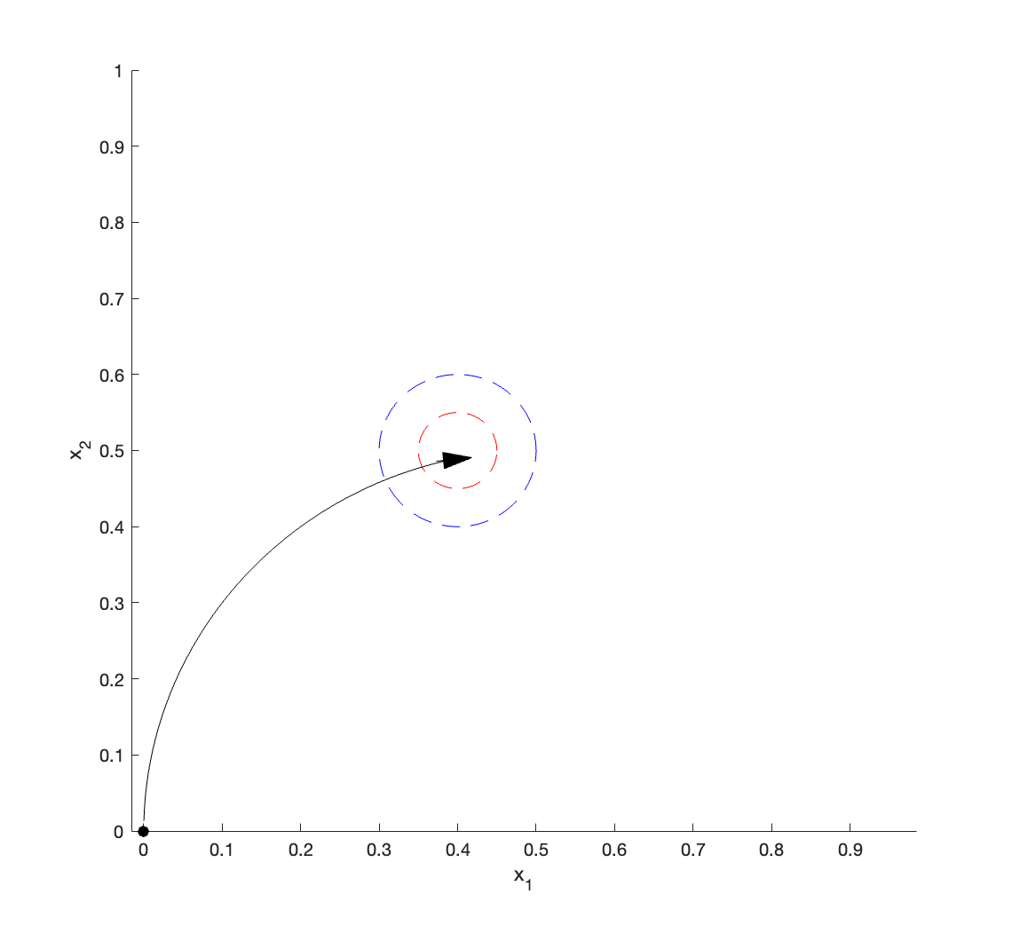
Refer to caption
(a) Step 1: (x1,x2)subscript𝑥1subscript𝑥2(x_{1},\,x_{2}) move to the red neighborhood
Refer to caption
(b) Step 2: (x1,x2)subscript𝑥1subscript𝑥2(x_{1},\,x_{2}) idle inside the red neighborhood.
Refer to caption
(c) Step 3: (x1,x2)subscript𝑥1subscript𝑥2(x_{1},\,x_{2}) drift inside the blue neighborhood.
Refer to caption
(d) Step 3: x3subscript𝑥3x_{3} move to the red neighborhood.
Refer to caption
(e) Step 4: (x1,x2)subscript𝑥1subscript𝑥2(x_{1},\,x_{2}) drift inside the blue neighborhood.
Refer to caption
(f) Step 4: x3subscript𝑥3x_{3} drift inside the blue neighborhood.
Figure 1: In these pictures, the blue region represents the target neighborhood, the red region represents the smaller neighborhood inside, and the black line represents the trajectory.

To control the projective process, our strategy is to split the control problem into two parts, one on the unit sphere, and the other one on the base manifold. To coordinate the two control problems, we use the topological property of the even-dimensional sphere, hairy ball theorem. First, we move the component on the sphere to the points where xX0vsubscript𝑥subscript𝑋0𝑣\nabla_{x}X_{0}v vanishes. Second, we use X0subscript𝑋0X_{0} and X1subscript𝑋1X_{1} to achieve the control in the (x1,x2)subscript𝑥1subscript𝑥2(x_{1},x_{2}) component of the base manifold. Finally, we finish the control problem on the sphere and the x3subscript𝑥3x_{3} component of the base manifold to close the argument.

Let us make a few observations. Before projecting onto the tangent plane of Sx𝕋3subscript𝑆𝑥superscript𝕋3S_{x}\mathbb{T}^{3}, the v𝑣v-component of X~0subscript~𝑋0\tilde{X}_{0} is

xX0v=[v3sinx3v3cosx30].subscript𝑥subscript𝑋0𝑣matrixsubscript𝑣3subscript𝑥3subscript𝑣3subscript𝑥30\nabla_{x}X_{0}\,v=\begin{bmatrix}-v_{3}\sin{x_{3}}&v_{3}\cos{x_{3}}&0\end{bmatrix}.

Using the diffusion vector field X~1subscript~𝑋1\tilde{X}_{1}, we can move instantaneously along the x3subscript𝑥3x_{3}-direction; therefore it makes sense to consider the following auxilliary vector fields by letting x3subscript𝑥3x_{3} be 00, π/2𝜋2\pi/2, π𝜋\pi and 3π/23𝜋23\pi/2,

Y0,1subscript𝑌01\displaystyle Y_{0,1} (1Πv)xX0(x1,x2,0)v=(1Πv)[0v30],absent1subscriptΠ𝑣subscript𝑥subscript𝑋0subscript𝑥1subscript𝑥20𝑣1subscriptΠ𝑣matrix0subscript𝑣30\displaystyle\coloneqq\left(1-\Pi_{v}\right)\nabla_{x}X_{0}(x_{1},x_{2},0)v=\left(1-\Pi_{v}\right)\begin{bmatrix}\phantom{-}0&\phantom{-}v_{3}&0\end{bmatrix},
Y0,2subscript𝑌02\displaystyle Y_{0,2} (1Πv)xX0(x1,x2,π/2)v=(1Πv)[v300],absent1subscriptΠ𝑣subscript𝑥subscript𝑋0subscript𝑥1subscript𝑥2𝜋2𝑣1subscriptΠ𝑣matrixsubscript𝑣300\displaystyle\coloneqq\left(1-\Pi_{v}\right)\nabla_{x}X_{0}(x_{1},x_{2},\pi/2)v=\left(1-\Pi_{v}\right)\begin{bmatrix}-v_{3}&\phantom{-}0&0\end{bmatrix},
Y0,3subscript𝑌03\displaystyle Y_{0,3} (1Πv)xX0(x1,x2,π)v=(1Πv)[0v30],absent1subscriptΠ𝑣subscript𝑥subscript𝑋0subscript𝑥1subscript𝑥2𝜋𝑣1subscriptΠ𝑣matrix0subscript𝑣30\displaystyle\coloneqq\left(1-\Pi_{v}\right)\nabla_{x}X_{0}(x_{1},x_{2},\pi)v=\left(1-\Pi_{v}\right)\begin{bmatrix}\phantom{-}0&-v_{3}&0\end{bmatrix},
Y0,4subscript𝑌04\displaystyle Y_{0,4} (1Πv)xX0(x1,x2,3π/2)v=(1Πv)[v300].absent1subscriptΠ𝑣subscript𝑥subscript𝑋0subscript𝑥1subscript𝑥23𝜋2𝑣1subscriptΠ𝑣matrixsubscript𝑣300\displaystyle\coloneqq\left(1-\Pi_{v}\right)\nabla_{x}X_{0}(x_{1},x_{2},3\pi/2)v=\left(1-\Pi_{v}\right)\begin{bmatrix}\phantom{-}v_{3}&\phantom{-}0&0\end{bmatrix}.

One can see that these vector fields vanish when v3=0subscript𝑣30v_{3}=0, and they allow us to move in the directions transversal to v3subscript𝑣3v_{3}-direction when v30subscript𝑣30v_{3}\neq 0. Next, we obtain from the v𝑣v-component of the diffusion vector fields,

Y1subscript𝑌1\displaystyle Y_{1} =v1[v3v1v3v21(v3)2],absentsubscript𝑣1matrixsubscript𝑣3subscript𝑣1subscript𝑣3subscript𝑣21superscriptsubscript𝑣32\displaystyle=v_{1}\,\begin{bmatrix}-v_{3}v_{1}&-v_{3}v_{2}&1-(v_{3})^{2}\end{bmatrix},
Y2subscript𝑌2\displaystyle Y_{2} =v2[v3v1v3v21(v3)2].absentsubscript𝑣2matrixsubscript𝑣3subscript𝑣1subscript𝑣3subscript𝑣21superscriptsubscript𝑣32\displaystyle=v_{2}\,\begin{bmatrix}-v_{3}v_{1}&-v_{3}v_{2}&1-(v_{3})^{2}\end{bmatrix}.

Define the auxiliary vector fields 𝒢=k=14Y0,kspan{Y1,Y2}𝒢superscriptsubscript𝑘14subscript𝑌0𝑘spansubscript𝑌1subscript𝑌2\mathcal{G}=\cup_{k=1}^{4}Y_{0,k}\,\cup\,\mbox{span}\left\{Y_{1},Y_{2}\right\} on 𝕊2superscript𝕊2\mathbb{S}^{2}. An important observation is

Theorem 4.6.

There exists T>0𝑇0T>0 such that

{v3=0}𝒜𝒢(v,T)v𝕊2.\{v_{3}=0\}\subseteq\mathcal{A}_{\mathcal{G}}(v,\leq T)\quad\forall v\in\mathbb{S}^{2}.

Moreover, ϵ>0for-allitalic-ϵ0\forall\epsilon>0

𝒜𝒢({v3=0},ϵ)¯=𝕊2.\overline{\mathcal{A}_{\mathcal{G}}(\{v_{3}=0\},\leq\epsilon)}=\mathbb{S}^{2}.

The control problem of the auxiliary family 𝒢𝒢\mathcal{G} is closely related to projective irreducibility. First, we show that we can approximate the integral curves of 𝒢𝒢\mathcal{G} arbitrarily well with the v𝑣v-component of vector fields in =X~0+𝒳~subscript~𝑋0~𝒳\mathcal{F}=\tilde{X}_{0}+\tilde{\mathcal{X}}.

Theorem 4.7.

Let w=(x,v)superscript𝑤superscript𝑥superscript𝑣w^{\prime}=(x^{\prime},v^{\prime}), w′′=(x′′,v′′)𝕊𝕋3superscript𝑤′′superscript𝑥′′superscript𝑣′′𝕊superscript𝕋3w^{\prime\prime}=(x^{\prime\prime},v^{\prime\prime})\in\mathbb{S}\mathbb{T}^{3}. Let

φtsubscript𝜑𝑡\displaystyle\varphi_{t} =v+0tY(φs)𝑑sforY{Y0,1,Y0,2,Y0,3,Y0,4}formulae-sequenceabsentsuperscript𝑣superscriptsubscript0𝑡𝑌subscript𝜑𝑠differential-d𝑠for𝑌subscript𝑌01subscript𝑌02subscript𝑌03subscript𝑌04\displaystyle=v^{\prime}+\int_{0}^{t}Y(\varphi_{s})\,ds\quad\mbox{for}\quad Y\in\{Y_{0,1},\,Y_{0,2},\,Y_{0,3},\,Y_{0,4}\}
ϕt/γsubscriptitalic-ϕ𝑡𝛾\displaystyle\phi_{t/\gamma} =v+0t/γγY(ϕs)𝑑sforYspan{Y1,Y2},γ.formulae-sequenceabsentsuperscript𝑣superscriptsubscript0𝑡𝛾𝛾𝑌subscriptitalic-ϕ𝑠differential-d𝑠forformulae-sequence𝑌spansubscript𝑌1subscript𝑌2𝛾\displaystyle=v^{\prime}+\int_{0}^{t/\gamma}\gamma Y(\phi_{s})\,ds\quad\mbox{for}\quad Y\in\mbox{span}\{Y_{1},Y_{2}\},\quad\gamma\in\mathbb{R}.

Denote M𝑀M and L𝐿L constants depending on the sup-norm and the Lipschitz constant of the vector fields. Then for all 0<δ10𝛿much-less-than10<\delta\ll 1, there exist controls α𝛼\alpha and β𝛽\beta such that ψt+δα(w′′)superscriptsubscript𝜓𝑡𝛿𝛼superscript𝑤′′\psi_{t+\delta}^{\alpha}(w^{\prime\prime}) and ψt/γβ(w′′)superscriptsubscript𝜓𝑡𝛾𝛽superscript𝑤′′\psi_{t/\gamma}^{\beta}(w^{\prime\prime}) are the integral curves of \mathcal{F} with initial w′′superscript𝑤′′w^{\prime\prime} under the controls α𝛼\alpha and β𝛽\beta respectively, and

|(ψt+δα,4,ψt+δα,5,ψt+δα,6)φt|superscriptsubscript𝜓𝑡𝛿𝛼4superscriptsubscript𝜓𝑡𝛿𝛼5superscriptsubscript𝜓𝑡𝛿𝛼6subscript𝜑𝑡\displaystyle\left|\left(\psi_{t+\delta}^{\alpha,4},\,\psi_{t+\delta}^{\alpha,5},\,\psi_{t+\delta}^{\alpha,6}\right)-\varphi_{t}\right| (|v′′v|+δM)eLtabsentsuperscript𝑣′′superscript𝑣𝛿𝑀superscript𝑒𝐿𝑡\displaystyle\leq\left(\left|v^{\prime\prime}-v^{\prime}\right|+\delta M\right)e^{Lt} (4.16)
|(ψt/γβ,4,ψt/γβ,5,ψt/γβ,6)ϕt/γ|superscriptsubscript𝜓𝑡𝛾𝛽4superscriptsubscript𝜓𝑡𝛾𝛽5superscriptsubscript𝜓𝑡𝛾𝛽6subscriptitalic-ϕ𝑡𝛾\displaystyle\left|\left(\psi_{t/\gamma}^{\beta,4},\,\psi_{t/\gamma}^{\beta,5},\,\psi_{t/\gamma}^{\beta,6}\right)-\phi_{t/\gamma}\right| (Mtγ+|vv′′|)e2Lt.absent𝑀𝑡𝛾superscript𝑣superscript𝑣′′superscript𝑒2𝐿𝑡\displaystyle\leq\left(\frac{Mt}{\gamma}+|v^{\prime}-v^{\prime\prime}|\right)e^{2Lt}. (4.17)
Proof.

If Y{Y0,1,Y0,2,Y0,3,Y0,4}𝑌subscript𝑌01subscript𝑌02subscript𝑌03subscript𝑌04Y\in\{Y_{0,1},\,Y_{0,2},\,Y_{0,3},\,Y_{0,4}\}, we may consider Y=Y0,1𝑌subscript𝑌01Y=Y_{0,1} without loss of generality. We pick the control α=(α1,,α5):[0,)5:𝛼superscript𝛼1superscript𝛼50superscript5\alpha=(\alpha^{1},\dotsc,\alpha^{5}):[0,\infty)\rightarrow\mathbb{R}^{5},

α(s)=(1+x3′′δ)𝐞1χ[0,δ)(s)𝐞1χ[δ,)(s)𝛼𝑠1superscriptsubscript𝑥3′′𝛿subscript𝐞1subscript𝜒0𝛿𝑠subscript𝐞1subscript𝜒𝛿𝑠\alpha(s)=-(1+\frac{x_{3}^{\prime\prime}}{\delta})\mathbf{e}_{1}\chi_{[0,\delta)}(s)-\mathbf{e}_{1}\chi_{[\delta,\infty)}(s)

where 𝐞15subscript𝐞1superscript5\mathbf{e}_{1}\in\mathbb{R}^{5} is the unit vector in the first entry; this control moves the x3subscript𝑥3x_{3} component from x3′′superscriptsubscript𝑥3′′x_{3}^{\prime\prime} to 00 within time δ𝛿\delta, and then fixes the x3subscript𝑥3x_{3} component after time δ𝛿\delta. Let

ψt+δα(w′′)superscriptsubscript𝜓𝑡𝛿𝛼superscript𝑤′′\displaystyle\psi_{t+\delta}^{\alpha}(w^{\prime\prime}) =w′′+0t+δX~0(ψsα(w′′))𝑑s+0t+δX~1(ψsα(w′′))α1(s)𝑑sabsentsuperscript𝑤′′superscriptsubscript0𝑡𝛿subscript~𝑋0superscriptsubscript𝜓𝑠𝛼superscript𝑤′′differential-d𝑠superscriptsubscript0𝑡𝛿subscript~𝑋1superscriptsubscript𝜓𝑠𝛼superscript𝑤′′superscript𝛼1𝑠differential-d𝑠\displaystyle=w^{\prime\prime}+\int_{0}^{t+\delta}\tilde{X}_{0}(\psi_{s}^{\alpha}(w^{\prime\prime}))\,ds+\int_{0}^{t+\delta}\tilde{X}_{1}(\psi_{s}^{\alpha}(w^{\prime\prime}))\,\alpha^{1}(s)ds
ψ~tsubscript~𝜓𝑡\displaystyle\tilde{\psi}_{t} =ψδα(w′′)+0tX~0(ψ~s)𝑑s0tX~1(ψ~s)𝑑sabsentsuperscriptsubscript𝜓𝛿𝛼superscript𝑤′′superscriptsubscript0𝑡subscript~𝑋0subscript~𝜓𝑠differential-d𝑠superscriptsubscript0𝑡subscript~𝑋1subscript~𝜓𝑠differential-d𝑠\displaystyle=\psi_{\delta}^{\alpha}(w^{\prime\prime})+\int_{0}^{t}\tilde{X}_{0}(\tilde{\psi}_{s})\,ds-\int_{0}^{t}\tilde{X}_{1}(\tilde{\psi}_{s})\,ds
φt(v)subscript𝜑𝑡superscript𝑣\displaystyle\varphi_{t}(v^{\prime}) =v+0tY0,1(φs(v))𝑑s,absentsuperscript𝑣superscriptsubscript0𝑡subscript𝑌01subscript𝜑𝑠superscript𝑣differential-d𝑠\displaystyle=v^{\prime}+\int_{0}^{t}Y_{0,1}(\varphi_{s}(v^{\prime}))\,ds,

where ψα(w′′)superscriptsubscript𝜓𝛼superscript𝑤′′\psi_{\cdot}^{\alpha}(w^{\prime\prime}) is the trajectory under the control α𝛼\alpha with initial w′′superscript𝑤′′w^{\prime\prime}, ψ~subscript~𝜓\tilde{\psi}_{\cdot} is an auxiliary trajectory for estimation, and φ(v)subscript𝜑superscript𝑣\varphi_{\cdot}(v^{\prime}) is the trajectory we aim to approximate. We have

(ψ~t4,ψ~t5,ψ~t6)φt=(ψδα,4(w′′),ψδα,6(w′′),ψδα,6(w′′))v+0tY0,1(ψ~s)𝑑s0tY0,1(φs)𝑑s,superscriptsubscript~𝜓𝑡4superscriptsubscript~𝜓𝑡5superscriptsubscript~𝜓𝑡6subscript𝜑𝑡superscriptsubscript𝜓𝛿𝛼4superscript𝑤′′superscriptsubscript𝜓𝛿𝛼6superscript𝑤′′superscriptsubscript𝜓𝛿𝛼6superscript𝑤′′superscript𝑣superscriptsubscript0𝑡subscript𝑌01subscript~𝜓𝑠differential-d𝑠superscriptsubscript0𝑡subscript𝑌01subscript𝜑𝑠differential-d𝑠\left(\tilde{\psi}_{t}^{4},\,\tilde{\psi}_{t}^{5},\,\tilde{\psi}_{t}^{6}\right)-\varphi_{t}=\left(\psi_{\delta}^{\alpha,4}(w^{\prime\prime}),\,\psi_{\delta}^{\alpha,6}(w^{\prime\prime}),\,\psi_{\delta}^{\alpha,6}(w^{\prime\prime})\right)-v^{\prime}+\int_{0}^{t}Y_{0,1}(\tilde{\psi}_{s})\,ds-\int_{0}^{t}Y_{0,1}(\varphi_{s})\,ds,

which by Grönwall inequality implies

|(ψ~t4,ψ~t5,ψ~t6)φt|superscriptsubscript~𝜓𝑡4superscriptsubscript~𝜓𝑡5superscriptsubscript~𝜓𝑡6subscript𝜑𝑡\displaystyle\left|\left(\tilde{\psi}_{t}^{4},\,\tilde{\psi}_{t}^{5},\,\tilde{\psi}_{t}^{6}\right)-\varphi_{t}\right| |(ψδα,4(w′′),ψδα,5(w′′),ψδα,6(w′′))v|eLtabsentsuperscriptsubscript𝜓𝛿𝛼4superscript𝑤′′superscriptsubscript𝜓𝛿𝛼5superscript𝑤′′superscriptsubscript𝜓𝛿𝛼6superscript𝑤′′superscript𝑣superscript𝑒𝐿𝑡\displaystyle\leq\left|\left(\psi_{\delta}^{\alpha,4}(w^{\prime\prime}),\,\psi_{\delta}^{\alpha,5}(w^{\prime\prime}),\,\psi_{\delta}^{\alpha,6}(w^{\prime\prime})\right)-v^{\prime}\right|e^{Lt} (4.18)
(|v′′v|+|0δX~0(ψsα(w′′))𝑑s|)eLt,absentsuperscript𝑣′′superscript𝑣superscriptsubscript0𝛿subscript~𝑋0superscriptsubscript𝜓𝑠𝛼superscript𝑤′′differential-d𝑠superscript𝑒𝐿𝑡\displaystyle\leq\left(\left|v^{\prime\prime}-v^{\prime}\right|+\left|\int_{0}^{\delta}\tilde{X}_{0}(\psi_{s}^{\alpha}(w^{\prime\prime}))\,ds\right|\right)e^{Lt}, (4.19)

where L𝐿L depends on the Lipschitz constant of the vector fields, and the integral involving X~1subscript~𝑋1\tilde{X}_{1} vanishes due to (X~14,X~15,X~16)=0superscriptsubscript~𝑋14superscriptsubscript~𝑋15superscriptsubscript~𝑋160(\tilde{X}_{1}^{4},\tilde{X}_{1}^{5},\tilde{X}_{1}^{6})=0. Also, we have

ψt+δα(w′′)=ψ~tsuperscriptsubscript𝜓𝑡𝛿𝛼superscript𝑤′′subscript~𝜓𝑡\psi_{t+\delta}^{\alpha}(w^{\prime\prime})=\tilde{\psi}_{t} (4.20)

by construction. Combining (4.19) and (4.20),

|(ψt+δα,4,ψt+δα,5,ψt+δα,6)φt|superscriptsubscript𝜓𝑡𝛿𝛼4superscriptsubscript𝜓𝑡𝛿𝛼5superscriptsubscript𝜓𝑡𝛿𝛼6subscript𝜑𝑡\displaystyle\left|\left(\psi_{t+\delta}^{\alpha,4},\,\psi_{t+\delta}^{\alpha,5},\,\psi_{t+\delta}^{\alpha,6}\right)-\varphi_{t}\right| =|(ψ~t4,ψ~t5,ψ~t6)φt|absentsuperscriptsubscript~𝜓𝑡4superscriptsubscript~𝜓𝑡5superscriptsubscript~𝜓𝑡6subscript𝜑𝑡\displaystyle=\left|\left(\tilde{\psi}_{t}^{4},\,\tilde{\psi}_{t}^{5},\,\tilde{\psi}_{t}^{6}\right)-\varphi_{t}\right|
(|v′′v|+|0δX~0(ψsα(w′′))𝑑s|)eLt(|v′′v|+δM)eLt,absentsuperscript𝑣′′superscript𝑣superscriptsubscript0𝛿subscript~𝑋0superscriptsubscript𝜓𝑠𝛼superscript𝑤′′differential-d𝑠superscript𝑒𝐿𝑡superscript𝑣′′superscript𝑣𝛿𝑀superscript𝑒𝐿𝑡\displaystyle\leq\left(\left|v^{\prime\prime}-v^{\prime}\right|+\left|\int_{0}^{\delta}\tilde{X}_{0}(\psi_{s}^{\alpha}(w^{\prime\prime}))\,ds\right|\right)e^{Lt}\leq\left(\left|v^{\prime\prime}-v^{\prime}\right|+\delta M\right)e^{Lt},

where M𝑀M depends on the sup norm of the vector fields; this shows (4.16).

If Y{Y1,Y2}𝑌subscript𝑌1subscript𝑌2Y\in\{Y_{1},Y_{2}\}, we may consider Y=Y1𝑌subscript𝑌1Y=Y_{1} without loss of generality. At least one of cos2x1′′superscript2superscriptsubscript𝑥1′′\cos^{2}{x_{1}^{\prime\prime}} and sin2x1′′superscript2superscriptsubscript𝑥1′′\sin^{2}{x_{1}^{\prime\prime}} is greater than or equal to 1/2121/2. For definiteness, we assume |cosx1′′|cos2(x1′′)1/2superscriptsubscript𝑥1′′superscript2superscriptsubscript𝑥1′′12\left|\cos{x_{1}^{\prime\prime}}\right|\geq\cos^{2}({x_{1}^{\prime\prime}})\neq 1/2. Given γ>0𝛾0\gamma>0, we pick the control β=(β1,,β5):[0,)5:𝛽superscript𝛽1superscript𝛽50superscript5\beta=(\beta^{1},\dotsc,\beta^{5}):[0,\infty)\rightarrow\mathbb{R}^{5},

β(s)=γcosx1′′𝐞𝟐,𝛽𝑠𝛾superscriptsubscript𝑥1′′subscript𝐞2\beta(s)=\frac{\gamma}{\cos{x_{1}^{\prime\prime}}}\mathbf{e_{2}},

where 𝐞25subscript𝐞2superscript5\mathbf{e}_{2}\in\mathbb{R}^{5} is the unit vector in the second entry. We then consider the following

ψt/γβsuperscriptsubscript𝜓𝑡𝛾𝛽\displaystyle\psi_{t/\gamma}^{\beta} =w′′+0t/γX~0(ψsβ)𝑑s+0t/γγcosx1′′X~2(ψsβ)𝑑sabsentsuperscript𝑤′′superscriptsubscript0𝑡𝛾subscript~𝑋0superscriptsubscript𝜓𝑠𝛽differential-d𝑠superscriptsubscript0𝑡𝛾𝛾superscriptsubscript𝑥1′′subscript~𝑋2superscriptsubscript𝜓𝑠𝛽differential-d𝑠\displaystyle=w^{\prime\prime}+\int_{0}^{t/\gamma}\tilde{X}_{0}(\psi_{s}^{\beta})\,ds+\int_{0}^{t/\gamma}\frac{\gamma}{\cos{x_{1}^{\prime\prime}}}\tilde{X}_{2}(\psi_{s}^{\beta})\,ds
ψ~t/γsubscript~𝜓𝑡𝛾\displaystyle\tilde{\psi}_{t/\gamma} =w′′+0t/γγcosx1′′X~2(ψ~s)𝑑sabsentsuperscript𝑤′′superscriptsubscript0𝑡𝛾𝛾superscriptsubscript𝑥1′′subscript~𝑋2subscript~𝜓𝑠differential-d𝑠\displaystyle=w^{\prime\prime}+\int_{0}^{t/\gamma}\frac{\gamma}{\cos{x_{1}^{\prime\prime}}}\tilde{X}_{2}(\tilde{\psi}_{s})\,ds
ϕt/γsubscriptitalic-ϕ𝑡𝛾\displaystyle\phi_{t/\gamma} =v+0t/γγY1(ϕs)𝑑s,absentsuperscript𝑣superscriptsubscript0𝑡𝛾𝛾subscript𝑌1subscriptitalic-ϕ𝑠differential-d𝑠\displaystyle=v^{\prime}+\int_{0}^{t/\gamma}\gamma Y_{1}(\phi_{s})\,ds,

where ψ/γβsuperscriptsubscript𝜓absent𝛾𝛽\psi_{\cdot/\gamma}^{\beta} is the trajectory under the control β𝛽\beta with initial w′′superscript𝑤′′w^{\prime\prime}, ψ~/γsubscript~𝜓absent𝛾\tilde{\psi}_{\cdot/\gamma} is an auxiliary trajectory for estimation, and ϕ/γsubscriptitalic-ϕabsent𝛾\phi_{\cdot/\gamma} is the trajectory we aim to approximate.

ψt/γβψ~t/γ=0t/γX~0(ψsβ)𝑑s+0t/γγcosx1′′X~2(ψsβ)𝑑s0t/γγcosx1′′X~2(ψ~s)𝑑s,superscriptsubscript𝜓𝑡𝛾𝛽subscript~𝜓𝑡𝛾superscriptsubscript0𝑡𝛾subscript~𝑋0superscriptsubscript𝜓𝑠𝛽differential-d𝑠superscriptsubscript0𝑡𝛾𝛾superscriptsubscript𝑥1′′subscript~𝑋2superscriptsubscript𝜓𝑠𝛽differential-d𝑠superscriptsubscript0𝑡𝛾𝛾superscriptsubscript𝑥1′′subscript~𝑋2subscript~𝜓𝑠differential-d𝑠\psi_{t/\gamma}^{\beta}-\tilde{\psi}_{t/\gamma}=\int_{0}^{t/\gamma}\tilde{X}_{0}(\psi_{s}^{\beta})\,ds+\int_{0}^{t/\gamma}\frac{\gamma}{\cos{x_{1}^{\prime\prime}}}\tilde{X}_{2}(\psi_{s}^{\beta})\,ds-\int_{0}^{t/\gamma}\frac{\gamma}{\cos{x_{1}^{\prime\prime}}}\tilde{X}_{2}(\tilde{\psi}_{s})\,ds,

which we may apply Grönwall inequality to get

|ψt/γβψ~t/γ|MtγeLt/|cosx1′′|.superscriptsubscript𝜓𝑡𝛾𝛽subscript~𝜓𝑡𝛾𝑀𝑡𝛾superscript𝑒𝐿𝑡superscriptsubscript𝑥1′′\left|\psi_{t/\gamma}^{\beta}-\tilde{\psi}_{t/\gamma}\right|\leq\frac{Mt}{\gamma}e^{Lt/|\cos{x_{1}^{\prime\prime}}|}. (4.21)

Also,

(ψ~t/γ,v4,ψ~t/γ,v5,ψ~t/γ,v6)superscriptsubscript~𝜓𝑡𝛾𝑣4superscriptsubscript~𝜓𝑡𝛾𝑣5superscriptsubscript~𝜓𝑡𝛾𝑣6\displaystyle\left(\tilde{\psi}_{t/\gamma,v}^{4},\,\tilde{\psi}_{t/\gamma,v}^{5},\,\tilde{\psi}_{t/\gamma,v}^{6}\right) ϕt/γ=v′′v+0t/γγcosx1′′(X~24,X~25,X~26)(ψ~s)𝑑s0t/γγY1(ϕs)𝑑ssubscriptitalic-ϕ𝑡𝛾superscript𝑣′′superscript𝑣superscriptsubscript0𝑡𝛾𝛾superscriptsubscript𝑥1′′superscriptsubscript~𝑋24superscriptsubscript~𝑋25superscriptsubscript~𝑋26subscript~𝜓𝑠differential-d𝑠superscriptsubscript0𝑡𝛾𝛾subscript𝑌1subscriptitalic-ϕ𝑠differential-d𝑠\displaystyle-\phi_{t/\gamma}=v^{\prime\prime}-v^{\prime}+\int_{0}^{t/\gamma}\frac{\gamma}{\cos{x_{1}^{\prime\prime}}}\left(\tilde{X}_{2}^{4},\,\tilde{X}_{2}^{5},\,\tilde{X}_{2}^{6}\right)(\tilde{\psi}_{s})\,ds-\int_{0}^{t/\gamma}\gamma Y_{1}(\phi_{s})\,ds
=v′′v+0t/γcosψ~s1cosx1′′γY1((ψ~t/γ,v4,ψ~t/γ,v5,ψ~t/γ,v6))𝑑s0t/γγY1(ϕs)𝑑sabsentsuperscript𝑣′′superscript𝑣superscriptsubscript0𝑡𝛾superscriptsubscript~𝜓𝑠1superscriptsubscript𝑥1′′𝛾subscript𝑌1superscriptsubscript~𝜓𝑡𝛾𝑣4superscriptsubscript~𝜓𝑡𝛾𝑣5superscriptsubscript~𝜓𝑡𝛾𝑣6differential-d𝑠superscriptsubscript0𝑡𝛾𝛾subscript𝑌1subscriptitalic-ϕ𝑠differential-d𝑠\displaystyle=v^{\prime\prime}-v^{\prime}+\int_{0}^{t/\gamma}\frac{\cos{\tilde{\psi}_{s}^{1}}}{\cos{x_{1}^{\prime\prime}}}\gamma Y_{1}\left((\tilde{\psi}_{t/\gamma,v}^{4},\,\tilde{\psi}_{t/\gamma,v}^{5},\,\tilde{\psi}_{t/\gamma,v}^{6})\right)\,ds-\int_{0}^{t/\gamma}\gamma Y_{1}(\phi_{s})\,ds
=v′′v+0t/γγ[Y1((ψ~t/γ,v4,ψ~t/γ,v5,ψ~t/γ,v6))Y1(ϕs)]𝑑s,absentsuperscript𝑣′′superscript𝑣superscriptsubscript0𝑡𝛾𝛾delimited-[]subscript𝑌1superscriptsubscript~𝜓𝑡𝛾𝑣4superscriptsubscript~𝜓𝑡𝛾𝑣5superscriptsubscript~𝜓𝑡𝛾𝑣6subscript𝑌1subscriptitalic-ϕ𝑠differential-d𝑠\displaystyle=v^{\prime\prime}-v^{\prime}+\int_{0}^{t/\gamma}\gamma\left[Y_{1}\left((\tilde{\psi}_{t/\gamma,v}^{4},\,\tilde{\psi}_{t/\gamma,v}^{5},\,\tilde{\psi}_{t/\gamma,v}^{6})\right)-Y_{1}(\phi_{s})\right]\,ds,

where the last equality is due to the x1subscript𝑥1x_{1}-component of X~2subscript~𝑋2\tilde{X}_{2} is zero, and so ψ~s1=x1′′superscriptsubscript~𝜓𝑠1superscriptsubscript𝑥1′′\tilde{\psi}_{s}^{1}=x_{1}^{\prime\prime}. Again, by Grönwall inequality

|(ψ~t/γ,v4,ψ~t/γ,v5,ψ~t/γ,v6)ϕt/γ||vv′′|eLt.superscriptsubscript~𝜓𝑡𝛾𝑣4superscriptsubscript~𝜓𝑡𝛾𝑣5superscriptsubscript~𝜓𝑡𝛾𝑣6subscriptitalic-ϕ𝑡𝛾superscript𝑣superscript𝑣′′superscript𝑒𝐿𝑡\left|\left(\tilde{\psi}_{t/\gamma,v}^{4},\,\tilde{\psi}_{t/\gamma,v}^{5},\,\tilde{\psi}_{t/\gamma,v}^{6}\right)-\phi_{t/\gamma}\right|\leq|v^{\prime}-v^{\prime\prime}|e^{Lt}. (4.22)

Combining (4.21) and (4.22), we have

|(ψt/γβ,4,ψt/γβ,5,ψt/γβ,6)ϕt/γ|superscriptsubscript𝜓𝑡𝛾𝛽4superscriptsubscript𝜓𝑡𝛾𝛽5superscriptsubscript𝜓𝑡𝛾𝛽6subscriptitalic-ϕ𝑡𝛾\displaystyle\left|\left(\psi_{t/\gamma}^{\beta,4},\,\psi_{t/\gamma}^{\beta,5},\,\psi_{t/\gamma}^{\beta,6}\right)-\phi_{t/\gamma}\right| |ψt/γβψ~t/γ|+|(ψ~t/γ,v4,ψ~t/γ,v5,ψ~t/γ,v6)ϕt/γ|absentsuperscriptsubscript𝜓𝑡𝛾𝛽subscript~𝜓𝑡𝛾superscriptsubscript~𝜓𝑡𝛾𝑣4superscriptsubscript~𝜓𝑡𝛾𝑣5superscriptsubscript~𝜓𝑡𝛾𝑣6subscriptitalic-ϕ𝑡𝛾\displaystyle\leq\left|\psi_{t/\gamma}^{\beta}-\tilde{\psi}_{t/\gamma}\right|+\left|\left(\tilde{\psi}_{t/\gamma,v}^{4},\,\tilde{\psi}_{t/\gamma,v}^{5},\,\tilde{\psi}_{t/\gamma,v}^{6}\right)-\phi_{t/\gamma}\right|
MtγeLt/|cosx1′′|+|vv′′|eLtabsent𝑀𝑡𝛾superscript𝑒𝐿𝑡superscriptsubscript𝑥1′′superscript𝑣superscript𝑣′′superscript𝑒𝐿𝑡\displaystyle\leq\frac{Mt}{\gamma}e^{Lt/|\cos{x}_{1}^{\prime\prime}|}+|v^{\prime}-v^{\prime\prime}|e^{Lt}
(Mtγ+|vv′′|)eLt/|cosx1′′|absent𝑀𝑡𝛾superscript𝑣superscript𝑣′′superscript𝑒𝐿𝑡superscriptsubscript𝑥1′′\displaystyle\leq\left(\frac{Mt}{\gamma}+|v^{\prime}-v^{\prime\prime}|\right)e^{Lt/|\cos{x}_{1}^{\prime\prime}|}
(Mtγ+|vv′′|)e2Lt.absent𝑀𝑡𝛾superscript𝑣superscript𝑣′′superscript𝑒2𝐿𝑡\displaystyle\leq\left(\frac{Mt}{\gamma}+|v^{\prime}-v^{\prime\prime}|\right)e^{2Lt}.

As a corollary, we have the integral curves of 𝒢𝒢\mathcal{G} can be approximated arbitrarily well by the projection of integral curves of \mathcal{F} on to 𝕊2superscript𝕊2\mathbb{S}^{2}.

Corollary 4.8.

Let φ:[0,T]𝕊2:subscript𝜑0𝑇superscript𝕊2\varphi_{\cdot}:[0,\,T]\rightarrow\mathbb{S}^{2} be an integral curve of 𝒢𝒢\mathcal{G} with initial vsuperscript𝑣v^{\prime}, and U𝑈U be an open neighborhood of φTsubscript𝜑𝑇\varphi_{T} in 𝕊2superscript𝕊2\mathbb{S}^{2}. Let x𝕋3superscript𝑥superscript𝕋3x^{\prime}\in\mathbb{T}^{3} and w=(x,v)superscript𝑤superscript𝑥superscript𝑣w^{\prime}=(x^{\prime},v^{\prime}). Then for all δ>0𝛿0\delta>0, there exists 0<TT+δ0superscript𝑇𝑇𝛿0<T^{\prime}\leq T+\delta, and an integral curve of \mathcal{F}, ψ:[0,T]𝕊𝕋3:𝜓0superscript𝑇𝕊superscript𝕋3\psi:[0,\,T^{\prime}]\rightarrow\mathbb{ST}^{3}, such that

  • ψ0=wsubscript𝜓0superscript𝑤\psi_{0}=w^{\prime},

  • (ψT4,ψT5,ψT6)Usuperscriptsubscript𝜓superscript𝑇4superscriptsubscript𝜓superscript𝑇5superscriptsubscript𝜓superscript𝑇6𝑈\left(\psi_{T^{\prime}}^{4},\,\psi_{T^{\prime}}^{5},\,\psi_{T^{\prime}}^{6}\right)\in U.

Proof.

Let 0=t0<t1<<tn=T0subscript𝑡0subscript𝑡1subscript𝑡𝑛𝑇0=t_{0}<t_{1}<\dotsc<t_{n}=T be the partition such that for m=1,,n𝑚1𝑛m=1,\dotsc,n

φ˙t=Ykm(φt)fortm1<t<tm,formulae-sequencesubscript˙𝜑𝑡subscript𝑌subscript𝑘𝑚subscript𝜑𝑡forsubscript𝑡𝑚1𝑡subscript𝑡𝑚\dot{\varphi}_{t}=Y_{k_{m}}(\varphi_{t})\quad\mbox{for}\quad t_{m-1}<t<t_{m},

and some Ykm𝒢subscript𝑌subscript𝑘𝑚𝒢Y_{k_{m}}\in\mathcal{G}. Given ϵ>0italic-ϵ0\epsilon>0, we will prove by induction on n𝑛n that there exist 0<TT+δ0superscript𝑇𝑇𝛿0<T^{\prime}\leq T+\delta and an integral curve ψ𝜓\psi of \mathcal{F} such that

|(ψT4,ψT5,ψT6)φtn|<ϵ.superscriptsubscript𝜓superscript𝑇4superscriptsubscript𝜓superscript𝑇5superscriptsubscript𝜓superscript𝑇6subscript𝜑subscript𝑡𝑛italic-ϵ\left|\left(\psi_{T^{\prime}}^{4},\,\psi_{T^{\prime}}^{5},\,\psi_{T^{\prime}}^{6}\right)-\varphi_{t_{n}}\right|<\epsilon. (4.23)

When n=1𝑛1n=1, there are two cases. For the first case,

φt1=v+0t1Yk1(φs)𝑑s,Yk1{Y0,1,Y0,2,Y0,3,Y0,4},formulae-sequencesubscript𝜑subscript𝑡1superscript𝑣superscriptsubscript0subscript𝑡1subscript𝑌subscript𝑘1subscript𝜑𝑠differential-d𝑠subscript𝑌subscript𝑘1subscript𝑌01subscript𝑌02subscript𝑌03subscript𝑌04\varphi_{t_{1}}=v^{\prime}+\int_{0}^{t_{1}}Y_{k_{1}}(\varphi_{s})\,ds,\qquad Y_{k_{1}}\in\left\{Y_{0,1},\,Y_{0,2},\,Y_{0,3},\,Y_{0,4}\right\},

then we can apply Theorem 4.7 and the fact that (ψ04,ψ05,ψ06)=vsuperscriptsubscript𝜓04superscriptsubscript𝜓05superscriptsubscript𝜓06superscript𝑣\left(\psi_{0}^{4},\,\psi_{0}^{5},\,\psi_{0}^{6}\right)=v^{\prime} to get a control α𝛼\alpha such that

|(ψt1+δα,4,ψt1+δα,5,ψt1+δα,6)φt1|δMeLt1,superscriptsubscript𝜓subscript𝑡1𝛿𝛼4superscriptsubscript𝜓subscript𝑡1𝛿𝛼5superscriptsubscript𝜓subscript𝑡1𝛿𝛼6subscript𝜑subscript𝑡1𝛿𝑀superscript𝑒𝐿subscript𝑡1\left|\left(\psi_{t_{1}+\delta}^{\alpha,4},\,\psi_{t_{1}+\delta}^{\alpha,5},\,\psi_{t_{1}+\delta}^{\alpha,6}\right)-\varphi_{t_{1}}\right|\leq\delta Me^{Lt_{1}},

where δ>0𝛿0\delta>0 can be arbitrarily small, and the claim is satisfied by taking δ=ϵM1eLt1𝛿italic-ϵsuperscript𝑀1superscript𝑒𝐿subscript𝑡1\delta=\epsilon M^{-1}e^{-Lt_{1}}. For the second case

φt1=v+0t1cYk1(φs)𝑑s,candYk1{Y1,Y2},formulae-sequencesubscript𝜑subscript𝑡1superscript𝑣superscriptsubscript0subscript𝑡1𝑐subscript𝑌subscript𝑘1subscript𝜑𝑠differential-d𝑠formulae-sequence𝑐andsubscript𝑌subscript𝑘1subscript𝑌1subscript𝑌2\varphi_{t_{1}}=v^{\prime}+\int_{0}^{t_{1}}cY_{k_{1}}(\varphi_{s})\,ds,\qquad c\in\mathbb{R}\quad\mbox{and}\quad Y_{k_{1}}\in\left\{Y_{1},\,Y_{2}\right\},

and for γ1much-greater-than𝛾1\gamma\gg 1 we can consider the accelerated version of the integral curve,

ϕt1/γ=v+0t1/γγcYk1(ϕs)𝑑s.subscriptitalic-ϕsubscript𝑡1𝛾superscript𝑣superscriptsubscript0subscript𝑡1𝛾𝛾𝑐subscript𝑌subscript𝑘1subscriptitalic-ϕ𝑠differential-d𝑠\phi_{t_{1}/\gamma}=v^{\prime}+\int_{0}^{t_{1}/\gamma}\gamma cY_{k_{1}}(\phi_{s})\,ds.

Then we can apply Theorem 4.7 and the fact that (ψ04,ψ05,ψ06)=vsuperscriptsubscript𝜓04superscriptsubscript𝜓05superscriptsubscript𝜓06superscript𝑣\left(\psi_{0}^{4},\,\psi_{0}^{5},\,\psi_{0}^{6}\right)=v^{\prime} to get a control β𝛽\beta such that

|(ψt1/γβ,4,ψt1/γβ,5,ψt1/γβ,6)ϕt1/γ|Mt1γe2Lt1,superscriptsubscript𝜓subscript𝑡1𝛾𝛽4superscriptsubscript𝜓subscript𝑡1𝛾𝛽5superscriptsubscript𝜓subscript𝑡1𝛾𝛽6subscriptitalic-ϕsubscript𝑡1𝛾𝑀subscript𝑡1𝛾superscript𝑒2𝐿subscript𝑡1\left|\left(\psi_{t_{1}/\gamma}^{\beta,4},\,\psi_{t_{1}/\gamma}^{\beta,5},\,\psi_{t_{1}/\gamma}^{\beta,6}\right)-\phi_{t_{1}/\gamma}\right|\leq\frac{Mt_{1}}{\gamma}e^{2Lt_{1}},

where γ>0𝛾0\gamma>0 can be arbitrarily large, and the claim is satisfied by taking γ=ϵ1Mt1exp(2Lt1)𝛾superscriptitalic-ϵ1𝑀subscript𝑡12𝐿subscript𝑡1\gamma=\epsilon^{-1}Mt_{1}\exp{(2Lt_{1})}. Therefore, the base case is proved.

Now, assume the hypothesis is true for n=l𝑛𝑙n=l, so there exists T′′>0superscript𝑇′′0T^{\prime\prime}>0 such that

|(ψT′′4,ψT′′5,ψT′′6)φtl|<ϵ;superscriptsubscript𝜓superscript𝑇′′4superscriptsubscript𝜓superscript𝑇′′5superscriptsubscript𝜓superscript𝑇′′6subscript𝜑subscript𝑡𝑙italic-ϵ\left|\left(\psi_{T^{\prime\prime}}^{4},\,\psi_{T^{\prime\prime}}^{5},\,\psi_{T^{\prime\prime}}^{6}\right)-\varphi_{t_{l}}\right|<\epsilon;

we will prove that it is also true for n=l+1𝑛𝑙1n=l+1. By taking (ψT′′4,ψT′′5,ψT′′6)superscriptsubscript𝜓superscript𝑇′′4superscriptsubscript𝜓superscript𝑇′′5superscriptsubscript𝜓superscript𝑇′′6\left(\psi_{T^{\prime\prime}}^{4},\,\psi_{T^{\prime\prime}}^{5},\,\psi_{T^{\prime\prime}}^{6}\right) and φtlsubscript𝜑subscript𝑡𝑙\varphi_{t_{l}} as our new initial conditions, we apply Theorem 4.7 to extend ψ𝜓\psi to get either

|(ψT′′+δ4,ψT′′+δ5,ψT′′+δ6)φtl+1|(|(ψT′′4,ψT′′5,ψT′′6)φtl|+δM)eL(tl+1tl)superscriptsubscript𝜓superscript𝑇′′𝛿4superscriptsubscript𝜓superscript𝑇′′𝛿5superscriptsubscript𝜓superscript𝑇′′𝛿6subscript𝜑subscript𝑡𝑙1superscriptsubscript𝜓superscript𝑇′′4superscriptsubscript𝜓superscript𝑇′′5superscriptsubscript𝜓superscript𝑇′′6subscript𝜑subscript𝑡𝑙𝛿𝑀superscript𝑒𝐿subscript𝑡𝑙1subscript𝑡𝑙\left|\left(\psi_{T^{\prime\prime}+\delta}^{4},\,\psi_{T^{\prime\prime}+\delta}^{5},\,\psi_{T^{\prime\prime}+\delta}^{6}\right)-\varphi_{t_{l+1}}\right|\leq\left(\left|\left(\psi_{T^{\prime\prime}}^{4},\,\psi_{T^{\prime\prime}}^{5},\,\psi_{T^{\prime\prime}}^{6}\right)-\varphi_{t_{l}}\right|+\delta M\right)e^{L(t_{l+1}-t_{l})}

for δ>0𝛿0\delta>0 arbitrarily small, or

|(ψT′′+(tl+1tl)/γ4,ψT′′+(tl+1tl)/γ5,ψT′′+(tl+1tl)/γ6)ϕtl+1|(|(ψT′′4,ψT′′5,ψT′′6)φtl|+M(tl+1tl)γ)e2L(tl+1tl)superscriptsubscript𝜓superscript𝑇′′subscript𝑡𝑙1subscript𝑡𝑙𝛾4superscriptsubscript𝜓superscript𝑇′′subscript𝑡𝑙1subscript𝑡𝑙𝛾5superscriptsubscript𝜓superscript𝑇′′subscript𝑡𝑙1subscript𝑡𝑙𝛾6subscriptitalic-ϕsubscript𝑡𝑙1superscriptsubscript𝜓superscript𝑇′′4superscriptsubscript𝜓superscript𝑇′′5superscriptsubscript𝜓superscript𝑇′′6subscript𝜑subscript𝑡𝑙𝑀subscript𝑡𝑙1subscript𝑡𝑙𝛾superscript𝑒2𝐿subscript𝑡𝑙1subscript𝑡𝑙\left|\left(\psi_{T^{\prime\prime}+(t_{l+1}-t_{l})/\gamma}^{4},\,\psi_{T^{\prime\prime}+(t_{l+1}-t_{l})/\gamma}^{5},\,\psi_{T^{\prime\prime}+(t_{l+1}-t_{l})/\gamma}^{6}\right)-\phi_{t_{l+1}}\right|\\[3.0pt] \leq\left(\left|\left(\psi_{T^{\prime\prime}}^{4},\,\psi_{T^{\prime\prime}}^{5},\,\psi_{T^{\prime\prime}}^{6}\right)-\varphi_{t_{l}}\right|+\frac{M(t_{l+1}-t_{l})}{\gamma}\right)e^{2L(t_{l+1}-t_{l})}

for γ>0𝛾0\gamma>0 arbitrarily large. This concludes our proof. ∎

As a consequence, we have the controllability for the projective process. Let us see how it is done before we move on to prove theorem 4.5.

Theorem 4.9.

There exists T>0superscript𝑇0T^{\prime}>0 such that

𝒜(w,T)¯=𝕊𝕋3.¯subscript𝒜𝑤superscript𝑇𝕊superscript𝕋3\overline{\mathcal{A}_{\mathcal{F}}(w,T^{\prime})}=\mathbb{ST}^{3}.
Proof.

Suppose we want to obtain a control to go from w=(x,v)superscript𝑤superscript𝑥superscript𝑣w^{\prime}=(x^{\prime},\,v^{\prime}) to a neighborhood U𝑈U of w′′=(x′′,v′′)superscript𝑤′′superscript𝑥′′superscript𝑣′′w^{\prime\prime}=(x^{\prime\prime},\,v^{\prime\prime}); we may assume that U𝑈U is of the form U=(I1××I6)𝕋3×𝕊2𝑈subscript𝐼1subscript𝐼6superscript𝕋3superscript𝕊2U=\left(I_{1}\times\dotsc\times I_{6}\right)\,\cap\,\mathbb{T}^{3}\times\mathbb{S}^{2}, where Iksubscript𝐼𝑘I_{k}’s are open intervals for k=1,,6𝑘16k=1,\dotsc,6. By Theorem 4.6, there exists an integral curve of 𝒢𝒢\mathcal{G} with the partition 0=t0<t1<<tm=T10subscript𝑡0subscript𝑡1subscript𝑡𝑚subscript𝑇10=t_{0}<t_{1}<\dotsc<t_{m}=T_{1} such that

ϕ0=v,ϕT1(I4×I5×I6)𝕊2andϕT1ϵ1{v3=0},formulae-sequencesubscriptitalic-ϕ0superscript𝑣formulae-sequencesubscriptitalic-ϕsubscript𝑇1subscript𝐼4subscript𝐼5subscript𝐼6superscript𝕊2andsubscriptitalic-ϕsubscript𝑇1subscriptitalic-ϵ1subscript𝑣30\phi_{0}=v^{\prime},\quad\phi_{T_{1}}\in\left(I_{4}\times I_{5}\times I_{6}\right)\cap\mathbb{S}^{2}\quad\mbox{and}\quad\phi_{T_{1}-\epsilon_{1}}\in\{v_{3}=0\},

where ϵ1>0subscriptitalic-ϵ10\epsilon_{1}>0 can be arbitrarily small. By definition,

ϕ˙t=Yi𝒢forti1<t<ti,i=1,,m,formulae-sequencesubscript˙italic-ϕ𝑡subscript𝑌𝑖𝒢forsubscript𝑡𝑖1𝑡subscript𝑡𝑖𝑖1𝑚\dot{\phi}_{t}=Y_{i}\in\mathcal{G}\quad\mbox{for}\quad t_{i-1}<t<t_{i},\quad i=1,\dotsc,m,

and we can apply Corollary 4.8 to get an integral curve φ=(φ1,φ2,,φ6):[0,T2]𝕊𝕋3:𝜑superscript𝜑1superscript𝜑2superscript𝜑60subscript𝑇2𝕊superscript𝕋3\varphi=(\varphi^{1},\,\varphi^{2},\dotsc,\varphi^{6}):[0,\,T_{2}]\rightarrow\mathbb{ST}^{3} of ~~\tilde{\mathcal{F}} such that

  • (φ04,φ05,φ06)=vsuperscriptsubscript𝜑04superscriptsubscript𝜑05superscriptsubscript𝜑06superscript𝑣\left(\varphi_{0}^{4},\,\varphi_{0}^{5},\,\varphi_{0}^{6}\right)=v^{\prime}.

  • (φT24,φT25,φT26)(I4×I5×I6)𝕊2superscriptsubscript𝜑subscript𝑇24superscriptsubscript𝜑subscript𝑇25superscriptsubscript𝜑subscript𝑇26subscript𝐼4subscript𝐼5subscript𝐼6superscript𝕊2\left(\varphi_{T_{2}}^{4},\,\varphi_{T_{2}}^{5},\,\varphi_{T_{2}}^{6}\right)\in\left(I_{4}\times I_{5}\times I_{6}\right)\cap\mathbb{S}^{2}.

  • (φT2ϵ24,φT2ϵ25,φT2ϵ26){v3=0}superscriptsubscript𝜑subscript𝑇2subscriptitalic-ϵ24superscriptsubscript𝜑subscript𝑇2subscriptitalic-ϵ25superscriptsubscript𝜑subscript𝑇2subscriptitalic-ϵ26subscript𝑣30\left(\varphi_{T_{2}-\epsilon_{2}}^{4},\,\varphi_{T_{2}-\epsilon_{2}}^{5},\,\varphi_{T_{2}-\epsilon_{2}}^{6}\right)\in\{v_{3}=0\}, where ϵ2subscriptitalic-ϵ2\epsilon_{2} is a small positive number depending on ϵ1subscriptitalic-ϵ1\epsilon_{1}.

It is possible to achieve the third bullet point, since we can pick ϕitalic-ϕ\phi so that ϕu{v3>0}subscriptitalic-ϕ𝑢subscript𝑣30\phi_{u}\in\{v_{3}>0\} and ϕu{v3<0}subscriptitalic-ϕsuperscript𝑢subscript𝑣30\phi_{u^{\prime}}\in\{v_{3}<0\} for some u<T1ϵ1<u𝑢subscript𝑇1subscriptitalic-ϵ1superscript𝑢u<T_{1}-\epsilon_{1}<u^{\prime}. By approximating ϕitalic-ϕ\phi well enough, φ𝜑\varphi will have to cross {v3=0}subscript𝑣30\{v_{3}=0\} by continuity.

Now, observe that both

(X~04,X~05,X~06)=(X~14,X~15,X~16)=0superscriptsubscript~𝑋04superscriptsubscript~𝑋05superscriptsubscript~𝑋06superscriptsubscript~𝑋14superscriptsubscript~𝑋15superscriptsubscript~𝑋160\left(\tilde{X}_{0}^{4},\,\tilde{X}_{0}^{5},\,\tilde{X}_{0}^{6}\right)=\left(\tilde{X}_{1}^{4},\,\tilde{X}_{1}^{5},\,\tilde{X}_{1}^{6}\right)=0

for {(x,v)𝕋3×𝕊2:v3=0}conditional-set𝑥𝑣superscript𝕋3superscript𝕊2subscript𝑣30\left\{(x,v)\in\mathbb{T}^{3}\times\mathbb{S}^{2}:v_{3}=0\right\}; hence, we can use X~0subscript~𝑋0\tilde{X}_{0} and X~1subscript~𝑋1\tilde{X}_{1} to control the position in the x𝑥x-direction without changing the position in v𝑣v-direction, once we are in {(x,v)𝕋3×𝕊2:v3=0}conditional-set𝑥𝑣superscript𝕋3superscript𝕊2subscript𝑣30\left\{(x,v)\in\mathbb{T}^{3}\times\mathbb{S}^{2}:v_{3}=0\right\}. By Theorem 4.5, we construct an integral curve φ~:[0,T3+T2ϵ2]𝕊𝕋3:~𝜑0subscript𝑇3subscript𝑇2subscriptitalic-ϵ2𝕊superscript𝕋3\tilde{\varphi}:[0,\,T_{3}+T_{2}-\epsilon_{2}]\rightarrow\mathbb{ST}^{3} such that

  • φ~t=φtsubscript~𝜑𝑡subscript𝜑𝑡\tilde{\varphi}_{t}=\varphi_{t} for 0tT2ϵ20𝑡subscript𝑇2subscriptitalic-ϵ20\leq t\leq T_{2}-\epsilon_{2}.

  • (φ~t4,φ~t5,φ~t6)=(φ~T2ϵ24,φ~T2ϵ25,φ~T2ϵ26)superscriptsubscript~𝜑𝑡4superscriptsubscript~𝜑𝑡5superscriptsubscript~𝜑𝑡6superscriptsubscript~𝜑subscript𝑇2subscriptitalic-ϵ24superscriptsubscript~𝜑subscript𝑇2subscriptitalic-ϵ25superscriptsubscript~𝜑subscript𝑇2subscriptitalic-ϵ26\left(\tilde{\varphi}_{t}^{4},\,\tilde{\varphi}_{t}^{5},\,\tilde{\varphi}_{t}^{6}\right)=\left(\tilde{\varphi}_{T_{2}-\epsilon_{2}}^{4},\,\tilde{\varphi}_{T_{2}-\epsilon_{2}}^{5},\,\tilde{\varphi}_{T_{2}-\epsilon_{2}}^{6}\right) for T2ϵ2tT3+T2ϵ2subscript𝑇2subscriptitalic-ϵ2𝑡subscript𝑇3subscript𝑇2subscriptitalic-ϵ2T_{2}-\epsilon_{2}\leq t\leq T_{3}+T_{2}-\epsilon_{2}.

  • (φ~T3+T2ϵ21,φ~T3+T2ϵ22,φ~T3+T2ϵ23)I1×I2×I3superscriptsubscript~𝜑subscript𝑇3subscript𝑇2subscriptitalic-ϵ21superscriptsubscript~𝜑subscript𝑇3subscript𝑇2subscriptitalic-ϵ22superscriptsubscript~𝜑subscript𝑇3subscript𝑇2subscriptitalic-ϵ23subscript𝐼1subscript𝐼2subscript𝐼3\left(\tilde{\varphi}_{T_{3}+T_{2}-\epsilon_{2}}^{1},\,\tilde{\varphi}_{T_{3}+T_{2}-\epsilon_{2}}^{2},\,\tilde{\varphi}_{T_{3}+T_{2}-\epsilon_{2}}^{3}\right)\in I_{1}\times I_{2}\times I_{3}.

To finish our proof, first observe that there exists 0<ϵ3<ϵ20subscriptitalic-ϵ3subscriptitalic-ϵ20<\epsilon_{3}<\epsilon_{2} and open neighborhood U~~𝑈\tilde{U} of φ~T1+T2ϵ2subscript~𝜑subscript𝑇1subscript𝑇2subscriptitalic-ϵ2\tilde{\varphi}_{T_{1}+T_{2}-\epsilon_{2}} such that

𝒜X~0(U~,ϵ3)U.\mathcal{A}_{\tilde{X}_{0}}(\tilde{U},\leq\epsilon_{3})\subset U.

Again, we may assume U~~𝑈\tilde{U} is of the form U~=(I~1××I~6)𝕋3×𝕊2~𝑈subscript~𝐼1subscript~𝐼6superscript𝕋3superscript𝕊2\tilde{U}=(\tilde{I}_{1}\times\dotsc\times\tilde{I}_{6})\,\cap\,\mathbb{T}^{3}\times\mathbb{S}^{2}, where I~ksubscript~𝐼𝑘\tilde{I}_{k}’s are open intervals for k=1,,6𝑘16k=1,\dotsc,6. We extend our integral curve to φ~:[0,T3+T2]𝕊𝕋3:~𝜑0subscript𝑇3subscript𝑇2𝕊superscript𝕋3\tilde{\varphi}:[0,\,T_{3}+T_{2}]\rightarrow\mathbb{ST}^{3} in the following steps:

  1. 1.

    If necessary, use Theorem 4.5 to obtain a control such that

    (φ~T3+T2ϵ31,φ~T3+T2ϵ32)I~1×I~2andφ~T3+T2ϵ2k=φ~T3+T2ϵ3kfork=4,5,6.formulae-sequencesuperscriptsubscript~𝜑subscript𝑇3subscript𝑇2subscriptitalic-ϵ31superscriptsubscript~𝜑subscript𝑇3subscript𝑇2subscriptitalic-ϵ32subscript~𝐼1subscript~𝐼2andformulae-sequencesuperscriptsubscript~𝜑subscript𝑇3subscript𝑇2subscriptitalic-ϵ2𝑘superscriptsubscript~𝜑subscript𝑇3subscript𝑇2subscriptitalic-ϵ3𝑘for𝑘456\left(\tilde{\varphi}_{T_{3}+T_{2}-\epsilon_{3}}^{1},\,\tilde{\varphi}_{T_{3}+T_{2}-\epsilon_{3}}^{2}\right)\in\tilde{I}_{1}\times\tilde{I}_{2}\quad\mbox{and}\quad\tilde{\varphi}_{T_{3}+T_{2}-\epsilon_{2}}^{k}=\tilde{\varphi}_{T_{3}+T_{2}-\epsilon_{3}}^{k}\quad\mbox{for}\quad k=4,5,6.
  2. 2.

    By Theorem 4.6 and Theorem 4.7, there exists some k{2,3,4,5}𝑘2345k\in\{2,3,4,5\} and some γ1much-greater-than𝛾1\gamma\gg 1 such that

    φ~T3+T2ϵ3+γ1=φ~T3+T2ϵ3+T3+T2ϵ3T3+T2ϵ3+1/γX~0(φ~s)±γX~k(φ~s)ds,subscript~𝜑subscript𝑇3subscript𝑇2subscriptitalic-ϵ3superscript𝛾1plus-or-minussubscript~𝜑subscript𝑇3subscript𝑇2subscriptitalic-ϵ3superscriptsubscriptsubscript𝑇3subscript𝑇2subscriptitalic-ϵ3subscript𝑇3subscript𝑇2subscriptitalic-ϵ31𝛾subscript~𝑋0subscript~𝜑𝑠𝛾subscript~𝑋𝑘subscript~𝜑𝑠𝑑𝑠\tilde{\varphi}_{T_{3}+T_{2}-\epsilon_{3}+\gamma^{-1}}=\tilde{\varphi}_{T_{3}+T_{2}-\epsilon_{3}}+\int_{T_{3}+T_{2}-\epsilon_{3}}^{T_{3}+T_{2}-\epsilon_{3}+1/\gamma}\tilde{X}_{0}(\tilde{\varphi}_{s})\pm\gamma\tilde{X}_{k}(\tilde{\varphi}_{s})\,ds,

    T3+T2ϵ3+γ1<T3+T2subscript𝑇3subscript𝑇2subscriptitalic-ϵ3superscript𝛾1subscript𝑇3subscript𝑇2T_{3}+T_{2}-\epsilon_{3}+\gamma^{-1}<T_{3}+T_{2}, and

    (φ~T3+T2ϵ3+γ14,φ~T3+T2ϵ3+γ15,φ~T3+T2ϵ3+γ16)I~4×I~5×I~6;superscriptsubscript~𝜑subscript𝑇3subscript𝑇2subscriptitalic-ϵ3superscript𝛾14superscriptsubscript~𝜑subscript𝑇3subscript𝑇2subscriptitalic-ϵ3superscript𝛾15superscriptsubscript~𝜑subscript𝑇3subscript𝑇2subscriptitalic-ϵ3superscript𝛾16subscript~𝐼4subscript~𝐼5subscript~𝐼6(\tilde{\varphi}_{T_{3}+T_{2}-\epsilon_{3}+\gamma^{-1}}^{4},\,\tilde{\varphi}_{T_{3}+T_{2}-\epsilon_{3}+\gamma^{-1}}^{5},\,\tilde{\varphi}_{T_{3}+T_{2}-\epsilon_{3}+\gamma^{-1}}^{6})\in\tilde{I}_{4}\times\tilde{I}_{5}\times\tilde{I}_{6};

    the sign in front of X~ksubscript~𝑋𝑘\tilde{X}_{k} depends on the direction we are moving.

  3. 3.

    Pick some γ~1much-greater-than~𝛾1\tilde{\gamma}\gg 1 such that

    φ~T3+T2ϵ3+γ1+γ~1=φ~T3+T2ϵ3+γ1+T3+T2ϵ3+1/γT3+T2ϵ3+1/γ+1/γ~X~0(φ~s)+γ~X~1(φ~s)ds,subscript~𝜑subscript𝑇3subscript𝑇2subscriptitalic-ϵ3superscript𝛾1superscript~𝛾1subscript~𝜑subscript𝑇3subscript𝑇2subscriptitalic-ϵ3superscript𝛾1superscriptsubscriptsubscript𝑇3subscript𝑇2subscriptitalic-ϵ31𝛾subscript𝑇3subscript𝑇2subscriptitalic-ϵ31𝛾1~𝛾subscript~𝑋0subscript~𝜑𝑠~𝛾subscript~𝑋1subscript~𝜑𝑠𝑑𝑠\tilde{\varphi}_{T_{3}+T_{2}-\epsilon_{3}+\gamma^{-1}+\tilde{\gamma}^{-1}}=\tilde{\varphi}_{T_{3}+T_{2}-\epsilon_{3}+\gamma^{-1}}+\int_{T_{3}+T_{2}-\epsilon_{3}+1/\gamma}^{T_{3}+T_{2}-\epsilon_{3}+1/\gamma+1/\tilde{\gamma}}\tilde{X}_{0}(\tilde{\varphi}_{s})+\tilde{\gamma}\tilde{X}_{1}(\tilde{\varphi}_{s})\,ds,

    T3+T2ϵ3+γ1+γ~1<T3+T2subscript𝑇3subscript𝑇2subscriptitalic-ϵ3superscript𝛾1superscript~𝛾1subscript𝑇3subscript𝑇2T_{3}+T_{2}-\epsilon_{3}+\gamma^{-1}+\tilde{\gamma}^{-1}<T_{3}+T_{2} and φ~T3+T2ϵ3+γ1+γ~1U~subscript~𝜑subscript𝑇3subscript𝑇2subscriptitalic-ϵ3superscript𝛾1superscript~𝛾1~𝑈\tilde{\varphi}_{T_{3}+T_{2}-\epsilon_{3}+\gamma^{-1}+\tilde{\gamma}^{-1}}\in\tilde{U}.

  4. 4.

    Finally, consider

    φ~T3+T2=φ~T3+T2ϵ3+γ1+γ~1+T3+T2ϵ3+1/γ+1/γ~T3+T2X~0(φ~s)𝑑s;subscript~𝜑subscript𝑇3subscript𝑇2subscript~𝜑subscript𝑇3subscript𝑇2subscriptitalic-ϵ3superscript𝛾1superscript~𝛾1superscriptsubscriptsubscript𝑇3subscript𝑇2subscriptitalic-ϵ31𝛾1~𝛾subscript𝑇3subscript𝑇2subscript~𝑋0subscript~𝜑𝑠differential-d𝑠\tilde{\varphi}_{T_{3}+T_{2}}=\tilde{\varphi}_{T_{3}+T_{2}-\epsilon_{3}+\gamma^{-1}+\tilde{\gamma}^{-1}}+\int_{T_{3}+T_{2}-\epsilon_{3}+1/\gamma+1/\tilde{\gamma}}^{T_{3}+T_{2}}\tilde{X}_{0}(\tilde{\varphi}_{s})\,ds;

    due to the way we pick ϵ3subscriptitalic-ϵ3\epsilon_{3}, we have φ~T3+T2Usubscript~𝜑subscript𝑇3subscript𝑇2𝑈\tilde{\varphi}_{T_{3}+T_{2}}\in U.

We break the proof of Theorem 4.6 into several lemmas. First, we observe that

N0={v3=0},N1={v1=0}andN2={v2=0}formulae-sequencesubscript𝑁0subscript𝑣30formulae-sequencesubscript𝑁1subscript𝑣10andsubscript𝑁2subscript𝑣20N_{0}=\{v_{3}=0\},\quad N_{1}=\{v_{1}=0\}\quad\mbox{and}\quad N_{2}=\{v_{2}=0\}

are the sets where the vector fields Y0,subscript𝑌0Y_{0,\cdot}, Y1subscript𝑌1Y_{1} and Y2subscript𝑌2Y_{2} vanish respectively.

Lemma 4.10.

The non-trivial orbits of Y1subscript𝑌1Y_{1} and Y2subscript𝑌2Y_{2} cover 𝕊2{v3=±1}superscript𝕊2subscript𝑣3plus-or-minus1\mathbb{S}^{2}\setminus\{v_{3}=\pm 1\},

𝕊2{v3=±1}=k=12{(v,t)𝕊2×:Yk(v)0}etYk(v),superscript𝕊2subscript𝑣3plus-or-minus1superscriptsubscript𝑘12subscriptconditional-set𝑣𝑡superscript𝕊2subscript𝑌𝑘𝑣0superscript𝑒𝑡subscript𝑌𝑘𝑣\mathbb{S}^{2}\setminus\{v_{3}=\pm 1\}=\bigcup_{k=1}^{2}\bigcup_{\left\{(v,t)\in\mathbb{S}^{2}\times\mathbb{R}:Y_{k}(v)\neq 0\right\}}e^{tY_{k}}(v),

and every non-trivial orbit of Y1subscript𝑌1Y_{1} and Y2subscript𝑌2Y_{2} intersects N0subscript𝑁0N_{0},

tetYk(v)N0,v{v𝕊2:Yk(v)0},k=1,2.formulae-sequencesubscript𝑡superscript𝑒𝑡subscript𝑌𝑘𝑣subscript𝑁0formulae-sequence𝑣conditional-set𝑣superscript𝕊2subscript𝑌𝑘𝑣0𝑘12\bigcup_{t\in\mathbb{R}}e^{tY_{k}}(v)\cap N_{0}\neq\emptyset,\quad v\in\left\{v\in\mathbb{S}^{2}:Y_{k}(v)\neq 0\right\},\,k=1,2.
Proof.

By symmetry, we may focus on studying the orbits of Y1subscript𝑌1Y_{1}. The orbits of Y1subscript𝑌1Y_{1} are partitioned into three parts,

N1,={v1<0},N1={v1=0}andN1,+={v1>0}.formulae-sequencesubscript𝑁1subscript𝑣10formulae-sequencesubscript𝑁1subscript𝑣10andsubscript𝑁1subscript𝑣10N_{1,-}=\{v_{1}<0\},\quad N_{1}=\{v_{1}=0\}\quad\mbox{and}\quad N_{1,+}=\{v_{1}>0\}.

The orbits in N1subscript𝑁1N_{1} are trivial, and the orbits in N1,subscript𝑁1N_{1,-} and N1,+subscript𝑁1N_{1,+} are symmetric; therefore, we can focus on analyzing N1,+subscript𝑁1N_{1,+}. In particular, we study the projected orbits to the (v1,v3)subscript𝑣1subscript𝑣3(v_{1},v_{3})-plane,

dv1dt𝑑subscript𝑣1𝑑𝑡\displaystyle\frac{dv_{1}}{dt} =v3(v1)2absentsubscript𝑣3superscriptsubscript𝑣12\displaystyle=-v_{3}(v_{1})^{2} (4.24)
dv3dt𝑑subscript𝑣3𝑑𝑡\displaystyle\frac{dv_{3}}{dt} =v1(1(v3)2).absentsubscript𝑣11superscriptsubscript𝑣32\displaystyle=v_{1}\left(1-(v_{3})^{2}\right). (4.25)

We include a picture of the vector field in Figure 2 for reference.
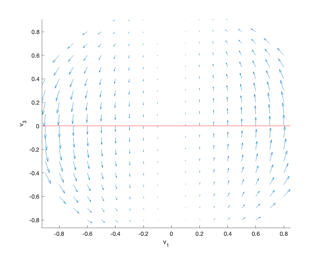
Refer to caption
Figure 2: A picture for the vector field (v3(v1)2,v1(1(v3))2)subscript𝑣3superscriptsubscript𝑣12subscript𝑣1superscript1subscript𝑣32(-v_{3}(v_{1})^{2},\,v_{1}(1-(v_{3}))^{2}).

To show that every orbit in N1,+subscript𝑁1N_{1},+ must pass through the equator N0subscript𝑁0N_{0}. Indeed,

d2v3dt2superscript𝑑2subscript𝑣3𝑑superscript𝑡2\displaystyle\frac{d^{2}v_{3}}{dt^{2}} =v3(v1)2(1(v3)2)2(v1)2v3(1(v3)2)absentsubscript𝑣3superscriptsubscript𝑣121superscriptsubscript𝑣322superscriptsubscript𝑣12subscript𝑣31superscriptsubscript𝑣32\displaystyle=-v_{3}(v_{1})^{2}(1-(v_{3})^{2})-2(v_{1})^{2}v_{3}(1-(v_{3})^{2})
=3(v1)2v3(1(v3)2),absent3superscriptsubscript𝑣12subscript𝑣31superscriptsubscript𝑣32\displaystyle=-3(v_{1})^{2}v_{3}(1-(v_{3})^{2}),

which is positive when v3<0subscript𝑣30v_{3}<0, zero when v3=0subscript𝑣30v_{3}=0 and negative when v3>0subscript𝑣30v_{3}>0; this suggests the system is accelerating upward in the lower half, and accelerating downward in the upper half. This and the fact that

dv3dt=v1(1(v3)2)>0inN1,+formulae-sequence𝑑subscript𝑣3𝑑𝑡subscript𝑣11superscriptsubscript𝑣320insubscript𝑁1\frac{dv_{3}}{dt}=v_{1}(1-(v_{3})^{2})>0\quad\mbox{in}\quad N_{1,+}

imply every orbit in N1,+subscript𝑁1N_{1,+} passes through N0subscript𝑁0N_{0}. ∎

Another thing we need is an estimate of how far right one can be when we reach N0subscript𝑁0N_{0}, if we start the system from, say, (v1,ϵ)N1,+subscript𝑣1italic-ϵsubscript𝑁1(v_{1},-\epsilon)\in N_{1,+}. Let t𝑡t be the time at which the system hits N0subscript𝑁0N_{0}. Then

0=v3(t)0subscript𝑣3𝑡\displaystyle 0=v_{3}(t) =ϵ+0tv1(s)(1(v3(s))2)𝑑sabsentitalic-ϵsuperscriptsubscript0𝑡subscript𝑣1𝑠1superscriptsubscript𝑣3𝑠2differential-d𝑠\displaystyle=-\epsilon+\int_{0}^{t}v_{1}(s)(1-(v_{3}(s))^{2})\,ds
ϵ+0tv1(0)(1ϵ2)𝑑s=ϵ+v1(0)(1ϵ2)t,absentitalic-ϵsuperscriptsubscript0𝑡subscript𝑣101superscriptitalic-ϵ2differential-d𝑠italic-ϵsubscript𝑣101superscriptitalic-ϵ2𝑡\displaystyle\leq-\epsilon+\int_{0}^{t}v_{1}(0)(1-\epsilon^{2})\,ds=-\epsilon+v_{1}(0)(1-\epsilon^{2})t,

where we used the fact that the system is accelerating upward in the lower part of N1,+subscript𝑁1N_{1,+}. This gives an upper bound for t𝑡t,

tϵv1(0)(1ϵ2).𝑡italic-ϵsubscript𝑣101superscriptitalic-ϵ2t\leq\frac{\epsilon}{v_{1}(0)(1-\epsilon^{2})}.

For v1(t)subscript𝑣1𝑡v_{1}(t), we have

v1(t)subscript𝑣1𝑡\displaystyle v_{1}(t) =v1(0)+0tv3(s)(v1(s))2dsabsentsubscript𝑣10superscriptsubscript0𝑡subscript𝑣3𝑠superscriptsubscript𝑣1𝑠2𝑑𝑠\displaystyle=v_{1}(0)+\int_{0}^{t}-v_{3}(s)(v_{1}(s))^{2}\,ds
v1(0)+0tϵ(v1(s))2𝑑sabsentsubscript𝑣10superscriptsubscript0𝑡italic-ϵsuperscriptsubscript𝑣1𝑠2differential-d𝑠\displaystyle\leq v_{1}(0)+\int_{0}^{t}\epsilon(v_{1}(s))^{2}\,ds
v1(0)+ϵtv1(0)+ϵ2v1(0)(1ϵ2).absentsubscript𝑣10italic-ϵ𝑡subscript𝑣10superscriptitalic-ϵ2subscript𝑣101superscriptitalic-ϵ2\displaystyle\leq v_{1}(0)+\epsilon t\leq v_{1}(0)+\frac{\epsilon^{2}}{v_{1}(0)(1-\epsilon^{2})}.

In particular, if we take (v1(0),v3(0))=(ϵ,ϵ)subscript𝑣10subscript𝑣30italic-ϵitalic-ϵ(v_{1}(0),v_{3}(0))=(\epsilon,-\epsilon), then

v1(t)ϵ+ϵ2ϵ(1ϵ2)<3ϵ,subscript𝑣1𝑡italic-ϵsuperscriptitalic-ϵ2italic-ϵ1superscriptitalic-ϵ23italic-ϵv_{1}(t)\leq\epsilon+\frac{\epsilon^{2}}{\epsilon(1-\epsilon^{2})}<3\epsilon, (4.26)

where the last inequality is true if we take for example ϵ2<1/2superscriptitalic-ϵ212\epsilon^{2}<1/2. Estimate (4.26) gives the following lemma.

Lemma 4.11.

Let 𝒢=span{Y1,Y2}superscript𝒢spansubscript𝑌1subscript𝑌2\mathcal{G}^{\prime}=\mbox{span}\{Y_{1},Y_{2}\}. For all t>0𝑡0t>0 and ϵ<1/9italic-ϵ19\epsilon<1/9,

N0𝒜𝒢({v3=±ϵ},t).N_{0}\subset\mathcal{A}_{\mathcal{G}^{\prime}}(\{v_{3}=\pm\epsilon\},\,\leq t).

Now we are ready to prove theorem 4.5. The main idea is to use Y0,subscript𝑌0Y_{0,\cdot} to go across orbits of Y1subscript𝑌1Y_{1} and Y2subscript𝑌2Y_{2} in a subset of S2superscript𝑆2S^{2}, then use Y1subscript𝑌1Y_{1} and Y2subscript𝑌2Y_{2} to move instantaneously within their orbits.

Proof.

Let Sϵ,±subscript𝑆italic-ϵplus-or-minusS_{\epsilon,\pm} be the stripes where ϵitalic-ϵ\epsilon will be determined later,

Sϵ,+=𝕊2{ϵv31ϵ}andSϵ,=𝕊2{1+ϵv3ϵ}.formulae-sequencesubscript𝑆italic-ϵsuperscript𝕊2italic-ϵsubscript𝑣31italic-ϵandsubscript𝑆italic-ϵsuperscript𝕊21italic-ϵsubscript𝑣3italic-ϵS_{\epsilon,+}=\mathbb{S}^{2}\cap\{\epsilon\leq v_{3}\leq 1-\epsilon\}\quad\mbox{and}\quad S_{\epsilon,-}=\mathbb{S}^{2}\cap\{-1+\epsilon\leq v_{3}\leq-\epsilon\}.

First, we show that there exists t1>0subscript𝑡10t_{1}>0 such that

Sϵ,+𝒜𝒢(v,t1)vSϵ,+andSϵ,𝒜𝒢(v,t1)vSϵ,.S_{\epsilon,+}\subseteq\mathcal{A}_{\mathcal{G}}\left(v,\,\leq t_{1}\right)\quad\forall v\in S_{\epsilon,+}\quad\mbox{and}\quad S_{\epsilon,-}\subseteq\mathcal{A}_{\mathcal{G}}\left(v,\,\leq t_{1}\right)\quad\forall v\in S_{\epsilon,-}. (4.27)

By symmetry, we focus on studying Sϵ,+subscript𝑆italic-ϵS_{\epsilon,+}. A few properties of the collection 𝒢𝒢\mathcal{G}:

  • Y0,1=Y0,3subscript𝑌01subscript𝑌03Y_{0,1}=-Y_{0,3} and Y0,2=Y0,4subscript𝑌02subscript𝑌04Y_{0,2}=-Y_{0,4}

  • For all vSϵ,+𝑣subscript𝑆italic-ϵv\in S_{\epsilon,+}, span{Y0,k,Yl}=Tv𝕊2subscript𝑌0𝑘subscript𝑌𝑙subscript𝑇𝑣superscript𝕊2\{Y_{0,k},\,Y_{l}\}=T_{v}\mathbb{S}^{2} for some (k,l){(1,1),(1,2),(2,1),(2,2)}𝑘𝑙11122122(k,l)\in\{(1,1),(1,2),(2,1),(2,2)\}.

Given vSϵ,+𝑣subscript𝑆italic-ϵv\in S_{\epsilon,+}, suppose span{Y0,k,Yl}=Tv𝕊2subscript𝑌0𝑘subscript𝑌𝑙subscript𝑇𝑣superscript𝕊2\{Y_{0,k},\,Y_{l}\}=T_{v}\mathbb{S}^{2}. For some neighborhood U𝑈U of 00 in 2superscript2\mathbb{R}^{2}, we may consider g:USϵ,+:𝑔𝑈subscript𝑆italic-ϵg:U\rightarrow S_{\epsilon,+}, defined as

g(t1,t2)=et2Ylet1Y0,k(v),𝑔subscript𝑡1subscript𝑡2superscript𝑒subscript𝑡2subscript𝑌𝑙superscript𝑒subscript𝑡1subscript𝑌0𝑘𝑣g(t_{1},t_{2})=e^{t_{2}Y_{l}}\circ e^{t_{1}Y_{0,k}}(v),

where the exponential denote the flow generated by the vector field. One can see that g(0,0)=v𝑔00𝑣g(0,0)=v, and by letting

φt(v)subscript𝜑𝑡𝑣\displaystyle\varphi_{t}(v) =v+0tY0,k(φs(v))𝑑sabsent𝑣superscriptsubscript0𝑡subscript𝑌0𝑘subscript𝜑𝑠𝑣differential-d𝑠\displaystyle=v+\int_{0}^{t}Y_{0,k}(\varphi_{s}(v))\,ds
ψt(v)subscript𝜓𝑡superscript𝑣\displaystyle\psi_{t}(v^{\prime}) =v+0tYl(ψs(v))𝑑s,absentsuperscript𝑣superscriptsubscript0𝑡subscript𝑌𝑙subscript𝜓𝑠superscript𝑣differential-d𝑠\displaystyle=v^{\prime}+\int_{0}^{t}Y_{l}(\psi_{s}(v^{\prime}))\,ds,

we have

g(t1,t2)=φt1(v)+0t2Yl(ψs(φt1(v)))𝑑s.𝑔subscript𝑡1subscript𝑡2subscript𝜑subscript𝑡1𝑣superscriptsubscript0subscript𝑡2subscript𝑌𝑙subscript𝜓𝑠subscript𝜑subscript𝑡1𝑣differential-d𝑠g(t_{1},t_{2})=\varphi_{t_{1}}(v)+\int_{0}^{t_{2}}Y_{l}(\psi_{s}(\varphi_{t_{1}}(v)))\,ds.

In particular,

t1g(0,0)subscriptsubscript𝑡1𝑔00\displaystyle\partial_{t_{1}}g(0,0) =φt1˙(v)+0t2(Ylφs)φt1˙(v)𝑑s|(t1,t2)=(0,0)=Y0,k(v)absent˙subscript𝜑subscript𝑡1𝑣evaluated-atsuperscriptsubscript0subscript𝑡2subscript𝑌𝑙subscript𝜑𝑠˙subscript𝜑subscript𝑡1𝑣differential-d𝑠subscript𝑡1subscript𝑡200subscript𝑌0𝑘𝑣\displaystyle=\left.\dot{\varphi_{t_{1}}}(v)+\int_{0}^{t_{2}}\nabla\left(Y_{l}\circ\varphi_{s}\right)\cdot\dot{\varphi_{t_{1}}}(v)\,ds\right|_{(t_{1},t_{2})=(0,0)}=Y_{0,k}(v)
t2g(0,0)subscriptsubscript𝑡2𝑔00\displaystyle\partial_{t_{2}}g(0,0) =Yl(v),absentsubscript𝑌𝑙𝑣\displaystyle=Y_{l}(v),

and the two vectors are linearly independent; hence, by inverse function theorem, there exists a neighborhood U~~𝑈\tilde{U} of 00 such that U~U~𝑈𝑈\tilde{U}\subseteq U and g:U~g(U~):𝑔~𝑈𝑔~𝑈g:\tilde{U}\rightarrow g(\tilde{U}) is a diffeomorphism. Define

t(v)=2max{|t1|,|t2|}(t1,t2)U~.t(v)=2\max\{|t_{1}|,|t_{2}|\}_{(t_{1},t_{2})\in\tilde{U}}.

Since Y0,ksubscript𝑌0𝑘Y_{0,k} and Y0,ksubscript𝑌0𝑘-Y_{0,k} are both in 𝒢𝒢\mathcal{G}, the above discussion implies that

g(U~)𝒜𝒢(v,t(v)).g(\tilde{U})\subseteq\mathcal{A}_{\mathcal{G}}\left(v,\leq t(v)\right).

For each vSϵ,+𝑣subscript𝑆italic-ϵv\in S_{\epsilon,+}, there exists a neighborhood of 00, Uv2subscript𝑈𝑣superscript2U_{v}\subseteq\mathbb{R}^{2}, and a diffeomorphism gv:Uvgv(Uv):subscript𝑔𝑣subscript𝑈𝑣subscript𝑔𝑣subscript𝑈𝑣g_{v}:U_{v}\rightarrow g_{v}(U_{v}) such that v=g(0,0)𝑣𝑔00v=g(0,0). Since Sϵ,+subscript𝑆italic-ϵS_{\epsilon,+} is compact, we may cover it with finitely many open neighborhood {gvi(Uvi)}i=1Nsuperscriptsubscriptsubscript𝑔subscript𝑣𝑖subscript𝑈subscript𝑣𝑖𝑖1𝑁\{g_{v_{i}}(U_{v_{i}})\}_{i=1}^{N}, and this shows

Sϵ,+𝒜𝒢(v,i=1Nt(vi))vSϵ,+.S_{\epsilon,+}\subseteq\mathcal{A}_{\mathcal{G}}\left(v,\leq\sum_{i=1}^{N}t(v_{i})\right)\quad\forall v\in S_{\epsilon,+}.

Denote

S+={v𝕊2:v30}andS={v𝕊2:v30}.formulae-sequencesubscript𝑆conditional-set𝑣superscript𝕊2subscript𝑣30andsubscript𝑆conditional-set𝑣superscript𝕊2subscript𝑣30S_{+}=\{v\in\mathbb{S}^{2}:v_{3}\geq 0\}\quad\mbox{and}\quad S_{-}=\{v\in\mathbb{S}^{2}:v_{3}\leq 0\}.

Next, we show that by picking ϵ1much-less-thanitalic-ϵ1\epsilon\ll 1 there exists t2>0subscript𝑡20t_{2}>0 such that

Sϵ,+𝒜𝒢(v,t2)vS+andSϵ,𝒜𝒢(v,t2)vS.S_{\epsilon,+}\cap\mathcal{A}_{\mathcal{G}}\left(v,\,\leq t_{2}\right)\neq\emptyset\quad\forall v\in S_{+}\quad\mbox{and}\quad S_{\epsilon,-}\cap\mathcal{A}_{\mathcal{G}}\left(v,\,\leq t_{2}\right)\neq\emptyset\quad\forall v\in S_{-}. (4.28)

By symmetry, we focus on studying S+subscript𝑆S_{+}. We observe that if 1ϵ<v3<11italic-ϵsubscript𝑣311-\epsilon<v_{3}<1, then by Lemma 4.10, for any δ>0𝛿0\delta>0

N0𝒜𝒢(v,δ)v{vS+:1ϵ<v3<1};N_{0}\cap\mathcal{A}_{\mathcal{G}}\left(v,\,\leq\delta\right)\neq\emptyset\quad\forall v\in\{v\in S_{+}:1-\epsilon<v_{3}<1\};

moreover, since the integral curves are continuous, it also implies

Sϵ,+𝒜𝒢(v,δ)v{vS+:1ϵ<v3<1}.S_{\epsilon,+}\cap\mathcal{A}_{\mathcal{G}}\left(v,\,\leq\delta\right)\neq\emptyset\quad\forall v\in\{v\in S_{+}:1-\epsilon<v_{3}<1\}.

If 0v3<ϵ0subscript𝑣3italic-ϵ0\leq v_{3}<\epsilon, we may without loss of generality assume v3=0subscript𝑣30v_{3}=0 due to Lemma 4.10. Then by picking ϵ<1/9italic-ϵ19\epsilon<1/9, we may apply Lemma 4.11 to conclude for all δ>0𝛿0\delta>0

Sϵ,+𝒜𝒢(v,δ)v{vS+:0v3<ϵ}.S_{\epsilon,+}\cap\mathcal{A}_{\mathcal{G}}\left(v,\,\leq\delta\right)\neq\emptyset\quad\forall v\in\{v\in S_{+}:0\leq v_{3}<\epsilon\}.

If v3=1subscript𝑣31v_{3}=1, since Y0,10subscript𝑌010Y_{0,1}\neq 0 at (0,0,1)S+001subscript𝑆(0,0,1)\in S_{+}, there exists some t2>0superscriptsubscript𝑡20t_{2}^{\prime}>0 such that

v=et2Y0,1(0,0,1)(0,0,1),superscript𝑣superscript𝑒superscriptsubscript𝑡2subscript𝑌01001001v^{\prime}=e^{t_{2}^{\prime}Y_{0,1}}(0,0,1)\neq(0,0,1),

and the previous two cases apply to vsuperscript𝑣v^{\prime}. In conclusion, we may take t2=t2+δsubscript𝑡2superscriptsubscript𝑡2𝛿t_{2}=t_{2}^{\prime}+\delta for arbitrary δ>0𝛿0\delta>0, and ϵ<1/9italic-ϵ19\epsilon<1/9 so that

Sϵ,+𝒜𝒢(v,t2)vS+.S_{\epsilon,+}\cap\mathcal{A}_{\mathcal{G}}\left(v,\,\leq t_{2}\right)\neq\emptyset\quad\forall v\in S_{+}.

Finally, by combining (4.27) and (4.28), we obtain

Sϵ,+𝒜𝒢(v,t1+t2)vS+andSϵ,𝒜𝒢(v,t1+t2)vS.S_{\epsilon,+}\subseteq\mathcal{A}_{\mathcal{G}}\left(v,\,\leq t_{1}+t_{2}\right)\quad\forall v\in S_{+}\quad\mbox{and}\quad S_{\epsilon,-}\subseteq\mathcal{A}_{\mathcal{G}}\left(v,\,\leq t_{1}+t_{2}\right)\quad\forall v\in S_{-}. (4.29)

By Lemma 4.11, (4.29) further implies for all δ>0𝛿0\delta>0,

N0𝒜𝒢(v,t1+t2+δ)v𝕊2.N_{0}\subseteq\mathcal{A}_{\mathcal{G}}\left(v,\,\leq t_{1}+t_{2}+\delta\right)\quad\forall v\in\mathbb{S}^{2}. (4.30)

By Lemma 4.10, (4.30) implies 𝒜𝒢(v,t1+t2+δ)\mathcal{A}_{\mathcal{G}}\left(v,\,\leq t_{1}+t_{2}+\delta\right) is dense in 𝕊2superscript𝕊2\mathbb{S}^{2} for all v𝑣v in 𝕊2superscript𝕊2\mathbb{S}^{2}. ∎

Appendix A Optimality for the decay bound in Theorem 1.1

In the following examples, we investigate the sharpness of the decay bound obtained in Theorem 1.1. The first example shows that the linear decay obtained in Theorem 1.1 is optimal in general. The second example shows that there are cases with sublinear decay. We consider diffusion processes on M=𝕋2𝑀superscript𝕋2M=\mathbb{T}^{2} with Euclidean metric.

Example A.1.

Let M=𝕋2𝑀superscript𝕋2M=\mathbb{T}^{2}. Consider the process

dxtϵ=ϵk=14Xk(xtϵ)dWk,𝑑superscriptsubscript𝑥𝑡italic-ϵitalic-ϵsuperscriptsubscript𝑘14subscript𝑋𝑘superscriptsubscript𝑥𝑡italic-ϵ𝑑subscript𝑊𝑘dx_{t}^{\epsilon}=\sqrt{\epsilon}\sum_{k=1}^{4}X_{k}(x_{t}^{\epsilon})\circ dW_{k},

where

X1=(10),X2=(01),X3=(sinx20)andX4=(0sinx1).formulae-sequencesubscript𝑋1matrix10formulae-sequencesubscript𝑋2matrix01formulae-sequencesubscript𝑋3matrixsubscript𝑥20andsubscript𝑋4matrix0subscript𝑥1X_{1}=\begin{pmatrix}1\\ 0\end{pmatrix},\quad X_{2}=\begin{pmatrix}0\\ 1\end{pmatrix},\quad X_{3}=\begin{pmatrix}\sin{x_{2}}\\ 0\end{pmatrix}\quad\mbox{and}\quad X_{4}=\begin{pmatrix}0\\ \sin{x_{1}}\end{pmatrix}.

A straightforward calculation shows it is associated with the projective process

dwtϵ=ϵk=14X~k(wtϵ)dWk,𝑑superscriptsubscript𝑤𝑡italic-ϵitalic-ϵsuperscriptsubscript𝑘14subscript~𝑋𝑘superscriptsubscript𝑤𝑡italic-ϵ𝑑subscript𝑊𝑘dw_{t}^{\epsilon}=\sqrt{\epsilon}\sum_{k=1}^{4}\tilde{X}_{k}(w_{t}^{\epsilon})\circ dW_{k},

where

X~1=(1000),X~2=(0100),X~3=(sinx20(1v12)v2cosx2v1v22cosx2)andX~4=(0sinx1v12v2cosx1v1(1v22)cosx1)formulae-sequencesubscript~𝑋1matrix1000formulae-sequencesubscript~𝑋2matrix0100formulae-sequencesubscript~𝑋3matrixsubscript𝑥201superscriptsubscript𝑣12subscript𝑣2subscript𝑥2subscript𝑣1superscriptsubscript𝑣22subscript𝑥2andsubscript~𝑋4matrix0subscript𝑥1superscriptsubscript𝑣12subscript𝑣2subscript𝑥1subscript𝑣11superscriptsubscript𝑣22subscript𝑥1\tilde{X}_{1}=\begin{pmatrix}1\\ 0\\ 0\\ 0\end{pmatrix},\quad\tilde{X}_{2}=\begin{pmatrix}0\\ 1\\ 0\\ 0\end{pmatrix},\quad\tilde{X}_{3}=\begin{pmatrix}\sin{x_{2}}\\ 0\\ (1-v_{1}^{2})v_{2}\cos{x_{2}}\\ -v_{1}v_{2}^{2}\cos{x_{2}}\end{pmatrix}\quad\mbox{and}\quad\tilde{X}_{4}=\begin{pmatrix}0\\ \sin{x_{1}}\\ -v_{1}^{2}v_{2}\cos{x_{1}}\\ v_{1}(1-v_{2}^{2})\cos{x_{1}}\end{pmatrix}

and we have divX~1=divX~2=0divsubscript~𝑋1divsubscript~𝑋20\mbox{div}\tilde{X}_{1}=\mbox{div}\tilde{X}_{2}=0, divX~3=4v1v2cosx2divsubscript~𝑋34subscript𝑣1subscript𝑣2subscript𝑥2\mbox{div}\tilde{X}_{3}=-4v_{1}v_{2}\cos{x_{2}} and divX~4=4v1v2cosx1divsubscript~𝑋44subscript𝑣1subscript𝑣2subscript𝑥1\mbox{div}\tilde{X}_{4}=-4v_{1}v_{2}\cos{x_{1}}. One can check that the processes are hypoelliptic and irreducible.

First, we show that λ1ϵsuperscriptsubscript𝜆1italic-ϵ\lambda_{1}^{\epsilon} decays exactly linearly as ϵ0italic-ϵ0\epsilon\rightarrow 0, and therefore our bound cannot be improved in general. Indeed,

0=~fϵ=ϵk(X~k)2fϵ=ϵ~1fϵfϵ=f1,formulae-sequence0superscript~superscript𝑓italic-ϵitalic-ϵsubscript𝑘superscriptsuperscriptsubscript~𝑋𝑘2superscript𝑓italic-ϵitalic-ϵsuperscriptsubscript~1superscript𝑓italic-ϵsuperscript𝑓italic-ϵsuperscript𝑓10=\tilde{\mathcal{L}}^{*}f^{\epsilon}=\epsilon\sum_{k}\left(\tilde{X}_{k}^{*}\right)^{2}f^{\epsilon}=\epsilon\tilde{\mathcal{L}}_{1}^{*}f^{\epsilon}\quad\Rightarrow\quad f^{\epsilon}=f^{1},

where we used the unique ergodicity. This implies

dλ1ϵ=ϵ2k=1r|X~kfϵ|2fϵ𝑑w=ϵ2k=1r|X~kf1|2f1𝑑w.𝑑superscriptsubscript𝜆1italic-ϵitalic-ϵ2superscriptsubscript𝑘1𝑟superscriptsuperscriptsubscript~𝑋𝑘superscript𝑓italic-ϵ2superscript𝑓italic-ϵdifferential-d𝑤italic-ϵ2superscriptsubscript𝑘1𝑟superscriptsuperscriptsubscript~𝑋𝑘superscript𝑓12superscript𝑓1differential-d𝑤d\lambda_{1}^{\epsilon}=\frac{\epsilon}{2}\sum_{k=1}^{r}\int\frac{|\tilde{X}_{k}^{*}f^{\epsilon}|^{2}}{f^{\epsilon}}\,dw=\frac{\epsilon}{2}\sum_{k=1}^{r}\int\frac{|\tilde{X}_{k}^{*}f^{1}|^{2}}{f^{1}}\,dw.

Next, we show that λ1ϵ>0superscriptsubscript𝜆1italic-ϵ0\lambda_{1}^{\epsilon}>0 for ϵ>0italic-ϵ0\epsilon>0. Denote gϵ=logfϵsuperscript𝑔italic-ϵsuperscript𝑓italic-ϵg^{\epsilon}=\log{f^{\epsilon}}. By contradiction, we assume λ1ϵ=0superscriptsubscript𝜆1italic-ϵ0\lambda_{1}^{\epsilon}=0 and therefore by (2.1),

X~kf=0fork=1,,4X~kg=divX~kfork=1,,4,formulae-sequencesuperscriptsubscript~𝑋𝑘𝑓0forformulae-sequence𝑘14formulae-sequencesubscript~𝑋𝑘𝑔divsubscript~𝑋𝑘for𝑘14\tilde{X}_{k}^{*}f=0\quad\mbox{for}\quad k=1,\dotsc,4\quad\Leftrightarrow\quad-\tilde{X}_{k}g=\mbox{div}\tilde{X}_{k}\quad\mbox{for}\quad k=1,\dotsc,4, (A.1)

where f𝑓f is the stationary density for wtϵsuperscriptsubscript𝑤𝑡italic-ϵw_{t}^{\epsilon}. Using (A.1) for k=1,2𝑘12k=1,2, we have g𝑔g is independent of x1subscript𝑥1x_{1} and x2subscript𝑥2x_{2}, and therefore

g=(00vg)andxkg=xkg=0fork=1,2.formulae-sequenceformulae-sequence𝑔matrix00subscript𝑣𝑔andsubscriptsubscript𝑥𝑘𝑔subscriptsubscript𝑥𝑘𝑔0for𝑘12\nabla g=\begin{pmatrix}0\\ 0\\ \nabla_{v}g\end{pmatrix}\quad\mbox{and}\quad\partial_{x_{k}}\nabla g=\nabla\partial_{x_{k}}g=0\quad\mbox{for}\quad k=1,2. (A.2)

Now, consider (A.1) for k=3𝑘3k=3, we have

((1v12)v2cosx2v1v22cosx2)vg=divX~3=0for(x,v)=(0,π2,22,22);formulae-sequencematrix1superscriptsubscript𝑣12subscript𝑣2subscript𝑥2subscript𝑣1superscriptsubscript𝑣22subscript𝑥2subscript𝑣𝑔divsubscript~𝑋30for𝑥𝑣0𝜋22222-\begin{pmatrix}(1-v_{1}^{2})v_{2}\cos{x_{2}}&-v_{1}v_{2}^{2}\cos{x_{2}}\end{pmatrix}\cdot\nabla_{v}g=\mbox{div}\tilde{X}_{3}=0\quad\mbox{for}\quad(x,v)=\left(0,\,\frac{\pi}{2},\,\frac{\sqrt{2}}{2},\,\frac{\sqrt{2}}{2}\right);

this in particular implies vg(0,π/2,2/2,2/2)=c(v1,v2)tsubscript𝑣𝑔0𝜋22222𝑐superscriptsubscript𝑣1subscript𝑣2𝑡\nabla_{v}g(0,\pi/2,\sqrt{2}/2,\sqrt{2}/2)=c(v_{1},\,v_{2})^{t} for some constant c𝑐c. However, this is absurd, since (A.2) would imply

vg=c(v1v2)for(x,v)=(0,x2,22,22),formulae-sequencesubscript𝑣𝑔𝑐matrixsubscript𝑣1subscript𝑣2for𝑥𝑣0subscript𝑥22222\nabla_{v}g=c\begin{pmatrix}v_{1}\\ v_{2}\end{pmatrix}\quad\mbox{for}\quad(x,v)=\left(0,\,x_{2},\,\frac{\sqrt{2}}{2},\,\frac{\sqrt{2}}{2}\right),

where x2subscript𝑥2x_{2} can be arbitrary. We may consider for instance x2=0subscript𝑥20x_{2}=0 to see (A.1) can not hold, since

divX~3=2,divsubscript~𝑋32\operatorname{div}\tilde{X}_{3}=-2,

which is not equal to

X~3g=24(11)22c(11)=0.subscript~𝑋3𝑔24matrix1122𝑐matrix110-\tilde{X}_{3}g=-\frac{\sqrt{2}}{4}\begin{pmatrix}1&-1\end{pmatrix}\cdot\frac{\sqrt{2}}{2}c\begin{pmatrix}1\\[3.0pt] 1\end{pmatrix}=0.

This is a contradction.

Example A.2.

This example is meant to explain why it is impossible to obtain an upper bound for

lim infϵ0λ1ϵϵ.subscriptlimit-infimumitalic-ϵ0superscriptsubscript𝜆1italic-ϵitalic-ϵ\liminf_{\epsilon\rightarrow 0}\frac{\lambda_{1}^{\epsilon}}{\epsilon}.

Let M=𝕋2𝑀superscript𝕋2M=\mathbb{T}^{2}. Consider the process

dxtϵ=X0(xtϵ)dt+ϵk=14Xk(xtϵ)dWk,𝑑superscriptsubscript𝑥𝑡italic-ϵsubscript𝑋0superscriptsubscript𝑥𝑡italic-ϵ𝑑𝑡italic-ϵsuperscriptsubscript𝑘14subscript𝑋𝑘superscriptsubscript𝑥𝑡italic-ϵ𝑑subscript𝑊𝑘dx_{t}^{\epsilon}=X_{0}(x_{t}^{\epsilon})\,dt+\sqrt{\epsilon}\sum_{k=1}^{4}X_{k}(x_{t}^{\epsilon})\circ dW_{k},

where Xksubscript𝑋𝑘X_{k} are the same as in Example A.1, and X0=X3subscript𝑋0subscript𝑋3X_{0}=X_{3}; the process is again elliptic and irreducible. By the results in [BBPS22], the shearing in the deterministic dynamics implies

lim infϵ0λ1ϵϵ=.subscriptlimit-infimumitalic-ϵ0superscriptsubscript𝜆1italic-ϵitalic-ϵ\liminf_{\epsilon\rightarrow 0}\frac{\lambda_{1}^{\epsilon}}{\epsilon}=\infty.

References