Blinding scheme for the scale-dependence bias signature of local primordial non-Gaussianity for DESI 2024
Abstract
The next generation of spectroscopic surveys is expected to achieve an unprecedented level of accuracy in the measurement of cosmological parameters. To avoid confirmation bias and thereby improve the reliability of these results, blinding procedures become a standard practice in the cosmological analyses of such surveys. Blinding is especially crucial when the impact of observational systematics is important relative to the cosmological signal, and a detection of that signal would have significant implications. This is the case for local primordial non-gaussianity, as probed by the scale-dependent bias of the galaxy power spectrum at large scales that are heavily sensitive to the dependence of the target selection on the imaging quality, known as imaging systematics. We propose a blinding method for the scale-dependent bias signature of local primordial non-gaussianity at the density field level which consists in generating a set of weights for the data that replicate the scale-dependent bias. The applied blinding is predictable, and can be straightforwardly combined with other catalog-level blinding procedures that have been designed for the baryon acoustic oscillation and redshift space distortion signals. The procedure is validated through simulations that replicate data from the first year of observation of the Dark Energy Spectroscopic Instrument, but may find applications to other upcoming spectroscopic surveys.
1 Introduction
In addition to providing tight constraints on the Universe expansion history, one of the major roles of current [1, 2] or future spectroscopic surveys [3, 4] is to provide an accurate measurement of the amount of primordial non-gaussianity (PNG) generated during inflation. In particular, these surveys will be focused on the well-known local PNG parameterized by [5] such that the primordial gravitational potential field reads
| (1.1) |
where is the Gaussian primordial potential field. A detection of would immediately rule out single field slow-roll inflation [6] as a valid paradigm to describe the early Universe.
Currently, the best constraints on local PNG are obtained from Planck data: [7]. To circumvent the cosmic variance limit of CMB observations, spectroscopic surveys use the enormous statistical power in the 3D galaxy clustering, probing a large volume of the Universe. A promising approach to constrain local PNG is through detecting the tiny imprint it leaves on the galaxy power spectrum at large scales, known as the scale-dependent bias on large scales [8, 9]. With this method, the best measurement leads to [10, 11, 12] and is obtained with the quasars of the extended Baryon Oscillation Spectroscopic Survey (eBOSS) [13].
Current spectroscopic surveys, as the Dark Energy Spectroscopic Instrument (DESI) [1, 14] or Euclid [2], are expected to constrain local PNG with similar accuracy to Planck. At the same time, future surveys are expected to reach a sensitivity of order unity [15], requiring robust and confirmation bias-free analyses.
Besides, the large-scale modes of the power spectrum used in the scale-dependent bias measurement may be strongly impacted by angular modes resulting from the dependence of the target selection to the imaging quality [16]. This dependence, known as imaging systematics, was the object of many studies carried out for the Sloan Digital Sky Survey (SDSS) [17, 18, 19, 20, 21, 22, 23, 24], the Dark Energy Survey (DES) [25, 26, 27, 28, 29], or more recently to prepare the upcoming DESI clustering analysis [30, 31, 32]. Correction schemes mostly rely on template fitting methods which need to be carefully calibrated to mitigate imaging systematics while avoiding overfitting. Overfitting indeed leads to a deficit of power at large scales that biases the analysis [33, 34]. Unfortunately, the efficiency of the systematic mitigation is typically validated on the actual data through several summary statistics, including the power spectrum itself, such that one may be influenced by previous detection (or non-detection) of PNG when tuning the systematic corrections, resulting in an important confirmation bias.
Similarly to the seminal blinding method for the baryon acoustic oscillation (BAO) and redshift-space distortion (RSD) analyses [35], we propose here a method that introduces at the catalog level a fake signal mimicking the scale-dependent bias that allows us to investigate the large scales of the power spectrum while protecting ourselves from confirmation bias. Section 2 describes the blinding scheme. Then, in Section 3, we validate the impact of this method on the power spectrum. In Section 4, we perform realistic tests with non-zero PNG simulations and validate the combination of the blinding method with the imaging systematic mitigation. We conclude in Section 5.
2 Theoretical description
In the following section we first introduce the signature of local PNG that we aim at blinding. We then describe the blinding scheme and its practical implementation, noting a shot noise correction is required to remove the sensitivity of the blinding scheme with the the tracer density.
2.1 Scale-dependent bias
Local primordial non-gaussianity leaves an imprint on the tracer power spectrum at large scales known as the scale-dependent bias [8, 9]:
| (2.1) |
where is the linear matter power spectrum, is a transfer function connecting the primordial gravitational field to the matter density perturbation such that
| (2.2) |
is the linear bias of the tracer and is the PNG bias given the response to the presence of local PNG of the tracer.
The transfer function can be computed directly as111We use CLASS [36] wrapped by https://github.com/cosmodesi/cosmoprimo:
| (2.3) |
where the primordial potential222 is normalized to to match the usual definition of [9]. power spectrum is defined as:
| (2.4) |
with is the spectral index and the amplitude of the initial power spectrum at . is the linear matter power spectrum such that has the famous scale dependency: [8].
The PNG bias can be expressed as with [9] (universal mass function) for tracers whose halo occupation distribution depends only on mass, although the pertinence of this description is currently discussed [37, 38, 39]. Since and are fully degenerate, in the following we assume the universal mass function to fix and we express the blinding amplitude in terms of .
2.2 Blinding scheme
2.2.1 Mimicking the scale-dependent bias
Our proposed blinding consists in adding a fake signal to the galaxy catalog, such that the measured power spectrum matches the large scale-dependent bias given in Eq. 2.1 for a specific value of , which we dub . This value is fixed randomly and is to remain unknown for all the data consistency tests performed during the analysis. Hence, the expected amount of PNG on the blinded data (assuming the chosen for the blinding is the true one) is where is the true value of the underlying cosmology and a random, fixed and unknown value.
Analyses of current spectroscopic surveys traditionally weight the data to correct for several observational effects as the completeness of the observations, the imaging dependence of the target selection or even the spectroscopic efficiency, see [40] for the description of the weights used in DESI. We alter the measured power spectrum at large scales by including in the catalog an additional set of weights, multiplied by the traditional ones to make them indistinguishable, such that , where is the galaxy density field and is the real space density field. The proposed weights are
| (2.5) |
where is the Fourier transform of
| (2.6) |
and is an estimate of . The quantities , and are computed at the effective redshift of the data (see, for instance, Eq. (3.5) of [12]). A wrong effective redshift will increase or decrease the real amount of added fake signal, such that the apparent value of will be slightly different. Note that a wrong bias will also alter the estimation of the real space density field. However all of these impacts will be neglected in the following, since we will use the correct effective redshift. Let us now detail the implementation of this blinding scheme.
2.2.2 Computing blinding weights
The real space density field in Eq. 2.6 is estimated by performing a reconstruction process, see [41] for a complete description. First, the density field is built by painting the particles (data and randoms) on a grid using the cloud-in-cell (CIC) assignment scheme. The smoothed Fourier-space density field is obtained with a Fast Fourier Transform (FFT) and a product with the Gaussian kernel
| (2.7) |
RSD displacements are then estimated from , assuming a fiducial bias and growth rate with the iterative FFT reconstruction algorithm [42] implemented in pyrecon333https://github.com/cosmodesi/pyrecon/tree/mpi. This branch is an MPI implementation and this is the only difference with the main branch.. Data particles are shifted back by the opposite of the RSD displacements, painted on a new grid, which is again Fourier-transformed, divided by and multiplied by another smoothing kernel to obtain an estimate of .
Finally, is read at the galaxy positions with the CIC scheme from the FFT of .
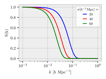
Since we only need to reconstruct the real-space density field at large scales (where PNG matters), we use a large smoothing radius . The corresponding kernel is displayed in Figure 1 for several values of . The larger the smoothing parameter, the more the fluctuations of the reconstructed density field on small scales (large ) is suppressed. The smoothing parameter allows us to control which scales will be affected by this blinding scheme, thereby preventing the BAO or RSD scales from being contaminated by these additional weights. While, the smoothing parameter controls the scale where the reconstruction is effective, see Eq. 2.12. More details on the effect of smoothing will be given in Section 3.4.
2.2.3 From galaxy catalog to the FKP field
Let us now describe the impact of the blinding weights obtained above on the estimated galaxy power spectrum. The FKP field [43], including the blinding weights above, reads:
| (2.8) | ||||
where we used the usual notation: and (resp. ) is the galaxy (resp. randoms) density. The randoms samples the survey geometry, more specifically the survey selection function , which is the ensemble average of the galaxy density: .
In Eq. 2.8, the term can be neglected since it is a second-order term in . As described in Appendix A, this assumption can be avoided by weighting the randoms instead of the data, though our tests have shown no practical difference.
One can also remark that, under this approximation, the expected value of is unchanged with the blinding scheme applied to the data. Indeed, the expected value reads:
| (2.9) | ||||
where as the result of the application of the linear operator to , of zero ensemble average.
This provides a simple way to test this approximation by computing the change in , which corresponds to the change in mean data weights. This change is minimal, typically about ; see for instance the data blinding weights displayed in Figure 9.
2.3 Shot noise correction
2.3.1 Power spectrum with the blinding scheme
Applying the blinding weights Eq. 2.5, the Fourier-space density field becomes where is the density field in redshift space and is the estimation of the field in real space. The associated power spectrum is, in the linear regime:
| (2.10) |
where is the shot noise.
Noting that, as described in Section 2.2.2, is an estimate of the reconstructed real space density field using a smoothing kernel , and then smoothed by , we find that and , in the linear regime, are
| (2.11) | ||||
| (2.12) |
2.3.2 Shot noise contribution
The shot noise terms (1/) in Eq. 2.11 and in Eq. 2.12 yield an extra contribution to the estimated power spectrum. In addition, shot noise varies with the local average density , i.e. the survey selection function. In particular, , and hence the shot noise, typically varies with the redshift and across the footprint due to the imaging dependence of the target selection444See, for instance, Figure 11 for a survey selection function.. The varying shot noise may then lead to different apparent values as a function of the redshift bin considered for the power spectrum estimation, preventing us from dedicated study, including internal consistency check on the blinded catalog, such as splitting the sample into several redshift bins. It is therefore crucial to correct for this shot noise effect.
To effectively treat this contribution, let us find to recover the expected value of the additional PNG power without the undesired shot noise term:
| (2.14) |
where (resp. ) corresponds to the zero shot noise part () of Eq. 2.11 (resp. Eq. 2.12). Solving the second-degree polynomial of Eq. 2.14 gives:
| (2.15) |
where the choice of the positive or negative solution of Eq. 2.15 will be discussed in Section 2.3.3.
The new parameter depends on both and via the shot noise term in and . To ensure that the amplitude of the PNG signal generated by the blinding scheme in the power spectrum does not depend on the local survey selection function, we want to keep the dependence on in and then for simplicity remove the dependence on . Hence, we choose a value of where the equality given in Eq. 2.14 holds and propose new, corrected, weights:
| (2.16) |
still with the Fourier transform of Eq. 2.6 and the corrective factor to suppress the shot noise contribution.
2.3.3 Positive or negative solution?
The reduced discriminant of Eq. 2.14 is always positive, as displayed in Figure 2, such that Eq. 2.14 has two real solutions.
When , it is clear with Eq. 2.6 that we need to choose the positive solution in Eq. 2.15 to have positive and mimic the positive behavior of local PNG. The choice of the solution in Eq. 2.15 for , is motivated to have a corrective factor () that is in , since is always positive by definition. We want to do not change the sign of the blinding signal and to reduce the amount of the blinding signal in presence of shot noise, see Eq. 2.10. This corrective factor is plotted in Figure 2 for different values of and for different values of shot noises. One can check that the corrective factors for the positive solution (blue/violet lines) are in for a reasonable value of as a function of the value of , while the corrective factors for negative solution (orange lines) do not respect this requirement.
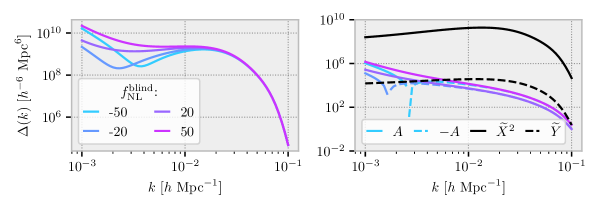
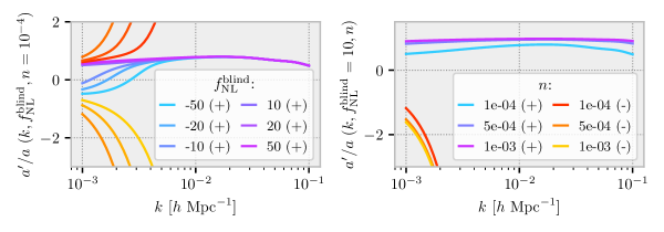
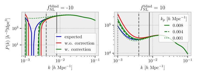
As explained in Section 2.3.2, we fix the corrective factor at a chosen value to be in for the considered range of blinding. This choice follows from the numerical study in Eq. 2.15 and the fact that in the following, we will limit our study to . Note that we expect to use a smaller range during the random choice of the blinding value since, for the upcoming DESI study with the first data release, a statistical precision of is expected, such that a lower range of blinding value will be used. Hence, when , we choose in order to de-bias the PNG signal at scales of interest. To avoid potential zero-crossing of the power spectrum when is negative, we choose a slightly higher value of . We use in all cases. The impact of the choice of on the theoretical description of the power spectrum given by Eq. 2.10 is shown in Figure 3. Note that the -range on which the scale-dependent bias will be fitted with the first data release of DESI will not include modes below .
2.4 Shot noise with data weights
For the shot noise correction to work, we need an appropriate estimate of the shot noise. We suggest using the same estimation as used in the power spectrum estimation555https://pypower.readthedocs.io/en/latest/api/api.html#pypower.fft_power.normalization, that is, in each cell of volume centered around the position :
| (2.17) |
where (resp. ) represents the weights of the data (resp. randoms).
The denominator is an estimation of the integral . We use instead of as the latter estimate is biased due to shot noise, which the former avoids under the assumption that data and randoms are uncorrelated.
2.5 Implementation
This method is implemented in mockfactory666https://github.com/cosmodesi/mockfactory/blob/main/mockfactory/blinding/catalog.py which is an MPI-parallel Python package that bundles utility functions to transform a cubic box simulation to a realistic observation mock, in particular, to reproduce the DESI observation. Although the official DESI blinding pipeline [45] does not use it, mockfactory also offers an implementation of the BAO and RSD blinding described in [35] under the same MPI framework.
3 Validation with Mocks
In this section we use simulations to validate the blinding scheme derived in the previous section. In particular, we first validate the theoretical description of the shot noise contribution, and then the proposed correction to remove this contribution from the blinding scheme. Finally, we emphasize the scales where the blinding scheme is effective and check the distribution of the blinding weights.
3.1 Mocks
To validate the PNG blinding scheme we use a FastPM [46] simulation generated to validate the DESI PNG analysis777We used the python version of FastPM: https://github.com/echaussidon/fastpm-python. We followed the parametrization of [47]. This simulation is a box of Gpc side length with 6000 meshes per side, i.e., particles leading to a dark matter particle mass of about M⊙. The initial dark matter field was generated at following the Planck18 cosmology [48] and using the "unitary method", which sets the initial white noise used to generate the initial density field to one, thus reducing the cosmological variance in the simulation [49]. Then, the particles evolved up to within 40 time steps. In the following, we use the snapshot .
From this snapshot, the halos are extracted with the popular Friend-of-Friend algorithm [50, 51] with a linking length of 0.2 times the mean interparticle distance. In particular, we use a slightly improved version of the MPI code [52]. Then, to emulate the linear bias of the eBOSS quasars sample observed in [53], we select all halos with a mass larger than , which corresponds to at least 178 dark matter particles.
Within this large box, the density of objects is . This full sample will also be denoted as a high-density sample. Two additional subsamples from this full sample are drawn to test the shot noise correction. The first one, of intermediate density, is obtained via a subsampling, yielding . The second one, of low density, is obtained by a subsampling, corresponding to . The shot noise is expected to be negligible in the high-density sample, while the low-density sample represents the typical density of the DESI QSO [54, 55, 56], where the shot noise cannot be neglected.
The power spectrum is measured with pypower888https://github.com/cosmodesi/pypower that implements the optimal FFT-based estimator of [57].
3.2 Model vs. mocks without shot noise corrective factor
Let us first apply the blinding scheme without adding the shot noise correction factor and validate the theoretical description given by Eq. 2.10. The blinded power spectra with different values of are displayed in Figure 4 for the high-density sample (left) and the low-density sample (right).
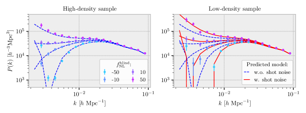
The blue dashed lines are the expected power spectra for the corresponding values (with a linear bias adjusted by eye) from Eq. 2.10 in the limit i.e. without the shot noise contribution. This is what the blinding should reproduce. The red lines correspond to Eq. 2.10 with the shot noise contribution. On the left, the blinding scheme is applied to a high-density sample where the shot noise can be neglected, and we do not display the corresponding red lines since they overlap almost perfectly with the blue lines. The blinding scheme is correctly described in this high-density configuration without the shot noise correction.
For the low-density sample (right), the blinding scheme’s impact on the power spectrum is accurately described only when the shot noise correction is included in the model prediction. Once the blinding applied, the blinded data will be fitted with the theory given in Eq. 2.1 without any shot noise correction such that not applying the correction at the blinding level yields a larger PNG signal. Hence, a coherent analysis of data split by their magnitudes or redshifts is made impossible if the shot noise varies across the survey since the blinding is applied only once to the entire sample.
3.3 Validation of the shot noise correction factor
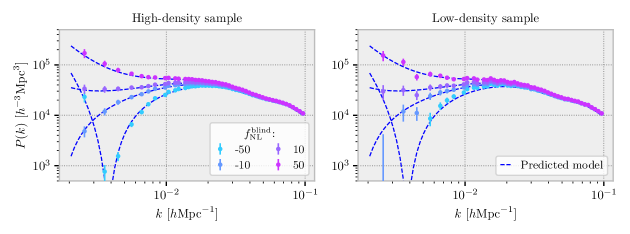
Let us test the final blinding scheme, which includes the shot noise correction factor. The blinded power spectra are shown in Figure 5 for high and low-density samples. Here, the predicted models are the power spectrum with the large scale-dependent bias given in Eq. 2.1 for (with a linear bias adjusted by eye). The blinding procedure recovers the desired shape of the power spectrum on large scales. In particular, the shot noise correction, given our choice of , works as expected up to the minimal scale of the fitting range i.e. .
One can validate this implementation by fitting the effective PNG signal introduced by the blinding scheme. We use the same parametrization as in the latest eBOSS measurement [10, 11, 12] where the power spectrum is expended on Legendre multipoles
| (3.1) |
with a simple model including the Kaiser effect, a damping factor for small scales, the scale-dependent bias, and a shot noise contribution:
| (3.2) |
The fits are performed with iminuit [58], and posterior samples are drawn with the zeus sampler [59, 60] wrapped into the desilike999https://github.com/cosmodesi/desilike framework101010A simple example of this model in this framework is given here:https://github.com/echaussidon/desilike/blob/main/nb/png_examples.ipynb. We fit only the monopole and the quadrupole for with a binning width of . The impact of the blinding scheme on the high-order multipoles is shown in Appendix B. We fix with the universal mass function assumption . Finally, the power spectrum covariance is computed analytically in the Gaussian approximation without window effect taking into account the DESI DR1 QSO number density, volume and linear bias.
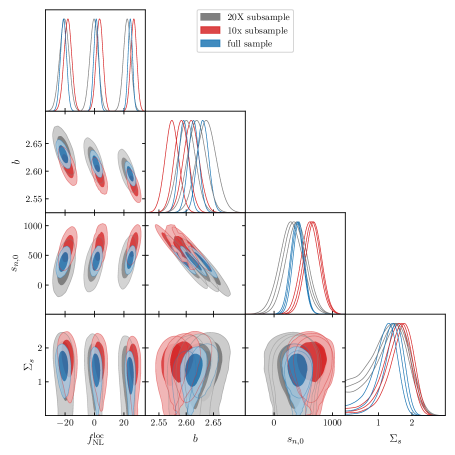
We fit the high-density sample (full sample) and the low-density sample ( subsampling), as well as the intermediate-density sample ( subsampling). The posteriors of are displayed in Figure 6 and the best-fit values with the errors from the posteriors for and in Figure 7. Note that, as expected, the errors decrease with the density of the sample.
As illustrated in Figure 6, fitted are consistent with input value for all density samples.


3.4 Blinded range of scales
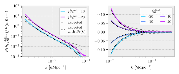
As illustrated in Figure 7, there is a shift in the measured bias as a function of the value. This discrepancy can be understood by examining the ratio between the blind and non-blind power spectrum monopoles displayed in Figure 8. The scale-dependent bias generated by the blinding scheme, given in Eq. 2.10 is altered by that erases the small scales. The measured ’high’- PNG signal is therefore damped by the kernel , as explained in Section 2.2.1.
The dashed lines in Figure 8 are the theoretical prediction without and the black dotted lines are the theoretical prediction () multiplied by . Note that this an approximation since also has a square contribution111111See the right term in Eq. 2.10. leading to the small discrepancy at between the prediction (black dotted lines) and the measured blinding power spectrum (colored lines). Hence, the blinding scheme slightly changes the amplitude of the power spectrum leading to a smaller effective bias.
The contribution of is not included in the fitted model used in Section 3.3, thereby explaining the different bias values displayed in Figure 6. This is not considered as an issue, as the galaxy bias is typically marginalized over, and the blinding scheme simulates the correct value of within error bars.
Another crucial point is the impact of the blinding is then negligible beyond , which should reduce its impact on BAO or RSD measurements, as demonstrated in Appendix C.
3.5 Distribution of blinding weights
Since this blinding scheme relies on applying additional weights to the data catalog, the variations in these weights must be small enough compared to those of other typical weights (e.g. to correct for observational systematics) to not provoke accidental unblinding.
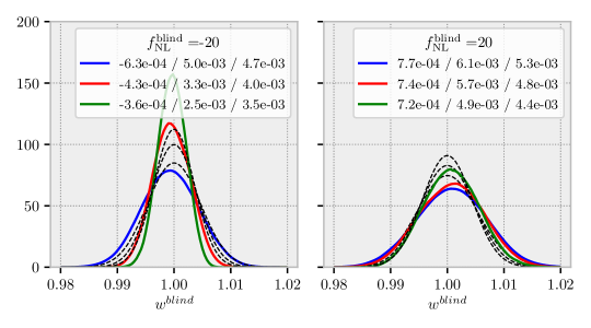
The expected standard deviation of the blinding weights, see Eq. 2.16, for constant density is
| (3.3) | ||||
where in the last equation we have approximated the contribution of to , in order to perform the integration.
Since the simulation box size is of finite size, the integration has to be performed only from with the box size to the Nyquist frequency.121212In fact, does not really matter since the integrand goes to really quickly for high .
Figure 9 shows the dispersion of the blinding weights for the corresponding values of ( on the left and on the right) for the different density samples. Note that the high density sample has a larger dispersion in blinding weights. This is expected since is bigger for higher density sample as displayed in the lower right panel of Figure 2.
For each configuration, the shift and standard deviation measured from the mocks and as predicted from Eq. 3.3 are given in the legend. The blinding weights have tiny offset (less than ) and very small standard deviation (less than ) such that they can be discreetly mixed with other weights without breaking the blinding procedure. Indeed, for comparison, realistic photometric systematic weights for DESI DR1 data have a standard deviation of , see [40].
4 Test with realistic cutsky mocks
The ultimate aim of this blinding procedure is to perform systematic and consistency tests on the data without any confirmation bias. Therefore, we have to check whether this method works also in the case of non-zero underlying PNG and if the added fake signal is insensitive to large angular scale imaging systematics and their mitigation. In the following, the blinding scheme is tested with realistic simulations that mimic the DESI DR1 QSO sample.
4.1 Realistic cutsky mocks
To build a more realistic simulation, the cubic box is transformed into a cutsky geometry where the density, the redshift distribution, the sky mask, as well as the completeness are matched to the expected DESI QSO DR1 sample [56]. All of these steps were performed with mockfactory. Note that despite the large size of this box (), one can only emulate either the North Galatic Cap (NGC) or the South Galactic Cap (SGC) of the DESI Survey. In the following, we decide to emulate the SGC part of the survey.
As mentioned above, the DESI QSO density corresponds to that of the low-density sample. Hence, 16 different subsamples can be extracted from the full sample. Although they are not entirely independent, we use the average on these 16 subsamples to reduce shot noise.
In the following, instead of using the analytical Gaussian approximation for the covariance matrix, we estimate it from 1000 EZMock fast simulations that match the DESI QSO DR1 SGC sample in the same manner as the cutsky FastPM. These EZMocks generated for DESI are very similar to the ones described in [61] (see [62] for an assessment of the covariance matrix from EZMocks).
Additionally, to account for the effect of the survey mask in the measured power spectra, all the fits are performed by convolving the theoretical power spectrum by the corresponding window function as explained in [63]. The window functions are also computed with pypower. We do not account for the negligible global integral constraint for this test.
4.2 Blinding with non-zero PNG simulations
First, we test the blinding procedure in the presence of a non-zero PNG signal. Similarly to the FastPM simulation described in Section 3.1, we have also produced one simulation with , from which 16 subsamples matching the DESI QSO DR1 SGC are extracted following the procedure described above. This simulation was produced with the same initial conditions, i.e., using the same initial density field, that is rescaled for the PNG case, to generate the initial particle distribution, see [64]. The fits are performed on the mean of these 16 subsamples without rescaling the mock-based covariance matrix.
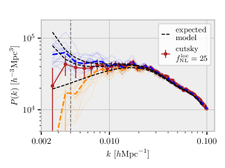
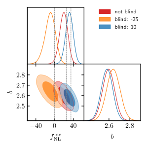
The DR1 SGC power spectra for the non-blinded case and blinding values of and the corresponding posteriors are displayed in Figure 10. The best-fit values are (non-blinded), (blinded + 10) and (blinded - 25) where the errors are the credible intervals. Note that the errors are smaller than expected for the real DESI analysis since the value of is computed with , see [9]. We mostly recover the expected behavior for the blinded power spectra down to the scale of interest (). Note that there is some small difference between the non-blinded power spectrum and the model, which is propagated to the blinded cases.
This difference in the non-blinded case is from the fact that halos in our FastPM simulations are extracted with a FoF halo finder which is known to produce halos that are not correctly described by the universal relation used for , see [65, 66] for an extensive study. One explanation could be that FoF algorithm creates non-spherical halos, while the universal relation for is derived from only spherical halos. This discrepancy will not impact our study since our simulation with has just a lower apparent amount of PNG signal.
4.3 Blinding with a mispecified survey selection function (remaining systematics)
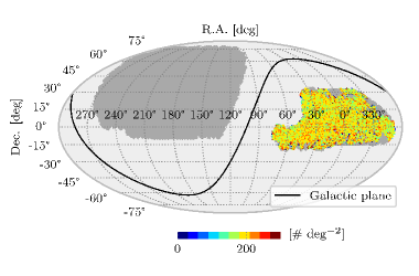
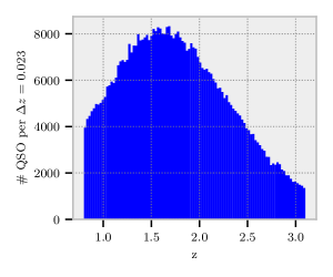
The ultimate test is to ensure that the blinding scheme is not altered by the presence of imaging systematics and by the mitigation applied for the correction. For this purpose, each subsample is contaminated by realistic imaging systematics. The footprint and the redshift distribution of one of this subsample are shown in Figure 11. Based on the density fluctuation in the sky observed in the DESI DR1 sample, we start with a subsample with a higher density than observed and we remove real objects in each pixel on the sky to match the density fluctuation at HEALPix [67] level with . We then apply the blinding scheme, and finally the imaging systematics are corrected either with the inverse of the contamination or with regressis131313https://github.com/echaussidon/regressis [32]. The measured value of is expected to recover the input .
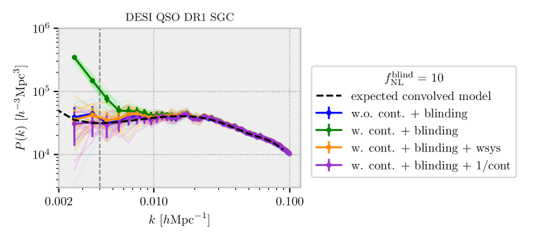
The means of the 16 subsamples of the power spectra for the different cases are shown in Figure 12. Note the importance of the imaging systematic mitigation in extracting the PNG signal.
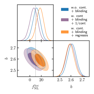
posteriors, for the mean of the 16 subsamples, are displayed in Figure 13. Here, we use the covariance matrix from the DR1 footprint instead of the one from the SGC footprint to reflect DR1 uncertainty. Note that in the fits we used since this is the value used during the blinding step. However, in the case of the QSO, one certainly wants to use instead of [9] during the fit, such that the expected errors with DESI DR1 will be a little bit larger than these ones. We recover the input blinding value well within the DR1 uncertainty both if no contamination is applied and including the imaging systematics, with the exact inverse correction. In the latter case, we obtain a slightly lower value of . The correction with regressis is slightly farther off (), but no fine-tuning of regressis was performed at this stage such that the imaging weights computed here are not optimal.
5 Conclusion
We have developed a method to blind the PNG signal that manifests as a large scale-dependent bias in the power spectrum. The proposed blinding scheme provides a set of weights to be applied to the data or the randoms such that the density field is altered at large scales to mimic a chosen scale-dependent bias. In particular, we have shown how shot noise propagates into our blinding scheme and how we can correct for it. This correction is significant and ensures a consistent fake PNG signal within a sample with varying density. We have also verified (in Appendix C) that the addition of this blinding does neither alter the measurement of the BAO and RSD parameters at the statistical accuracy of DR1 measurements nor alter the blinding setup for BAO and RSD.
As a result, this blinding was introduced into DESI’s clustering analysis pipeline, and since forecasts predict a sensitivity on of to at of confidence level with the DR1 data, we drew a single blinded random value for all the DESI tracers [45].
Although it was not the purpose here, the blinding scheme proposed could be tested and adapted to work for any other promising summary statistics as the CMB lensing [33], skew spectra [68, 69] or bispectrum [70]. Note that this blinding scheme will only alter the scale-dependent bias and is not able to blind the PNG signal coming from the matter density field. This is particularly relevant since, for instance, CMB lensing is not sensitive to the same systematics as the galaxy power spectrum and can help to provide an unbiased measurement. Finally, we emphasize also that this method can be easily adapted to any search of signal that changes the bias, for instance, the detection of relativistic contributions to galaxy clustering [71].
Data Availability
The blinding scheme is publicly available here: https://github.com/cosmodesi/mockfactory, as well as all the other tools mentioned in this article: https://github.com/cosmodesi/. All the material needed to reproduce all the figures of this publication is available here: https://doi.org/10.5281/zenodo.11270652.
Acknowledgments
This material is based upon work supported by the U.S. Department of Energy (DOE), Office of Science, Office of High-Energy Physics, under Contract No. DE–AC02–05CH11231, and by the National Energy Research Scientific Computing Center, a DOE Office of Science User Facility under the same contract. Additional support for DESI was provided by the U.S. National Science Foundation (NSF), Division of Astronomical Sciences under Contract No. AST-0950945 to the NSF’s National Optical-Infrared Astronomy Research Laboratory; the Science and Technology Facilities Council of the United Kingdom; the Gordon and Betty Moore Foundation; the Heising-Simons Foundation; the French Alternative Energies and Atomic Energy Commission (CEA); the National Council of Science and Technology of Mexico (CONACYT); the Ministry of Science and Innovation of Spain (MICINN), and by the DESI Member Institutions: https://www.desi.lbl.gov/collaborating-institutions. Any opinions, findings, and conclusions or recommendations expressed in this material are those of the author(s) and do not necessarily reflect the views of the U. S. National Science Foundation, the U. S. Department of Energy, or any of the listed funding agencies.
The authors are honored to be permitted to conduct scientific research on Iolkam Du’ag (Kitt Peak), a mountain with particular significance to the Tohono O’odham Nation.
References
- [1] DESI Collaboration, A. Aghamousa, J. Aguilar, S. Ahlen, S. Alam, L. E. Allen et al., The DESI Experiment Part I: Science,Targeting, and Survey Design, arXiv e-prints (2016) [1611.00036].
- [2] R. Scaramella, J. Amiaux, Y. Mellier, C. Burigana, C. S. Carvalho, J. C. Cuillandre et al., Euclid preparation: I. the Euclid Wide Survey, Astronomy and Astrophysics 662 (2022) [2108.01201].
- [3] O. Doré, J. Bock, M. Ashby, P. Capak, A. Cooray, R. de Putter et al., Cosmology with the SPHEREX All-Sky Spectral Survey, arXiv e-prints (2014) [1412.4872].
- [4] S. Ferraro, M. J. Wilson, M. Abidi, D. Alonso, B. Ansarinejad, R. Armstrong et al., Inflation and Dark Energy from spectroscopy at , arXiv e-prints (2019) [1903.09208].
- [5] E. Komatsu and D. N. Spergel, Acoustic signatures in the primary microwave background bispectrum, Physical Review D - Particles, Fields, Gravitation and Cosmology 63 (2001) 13 [astro-ph/0005036].
- [6] P. Creminelli and M. Zaldarriaga, A single-field consistency relation for the three-point function, Journal of Cosmology and Astroparticle Physics (2004) 101 [astro-ph/0407059].
- [7] Planck Collaboration, Y. Akrami, F. Arroja, M. Ashdown, J. Aumont, C. Baccigalupi et al., Planck 2018 results: IX. Constraints on primordial non-Gaussianity, Astronomy and Astrophysics 641 (2020) 24 [1905.05697].
- [8] N. Dalal, O. Doré, D. Huterer and A. Shirokov, Imprints of primordial non-Gaussianities on large-scale structure: Scale-dependent bias and abundance of virialized objects, Physical Review D - Particles, Fields, Gravitation and Cosmology 77 (2008) 1 [0710.4560].
- [9] A. Slosar, C. Hirata, U. Seljak, S. Ho and N. Padmanabhan, Constraints on local primordial non-Gaussianity from large scale structure, Journal of Cosmology and Astroparticle Physics 2008 (2008) [0805.3580].
- [10] E. Castorina, N. Hand, U. Seljak, F. Beutler, C. H. Chuang, C. Zhao et al., Redshift-weighted constraints on primordial non-Gaussianity from the clustering of the eBOSS DR14 quasars in Fourier space, Journal of Cosmology and Astroparticle Physics 2019 (2019) [1904.08859].
- [11] E.-M. Mueller, M. Rezaie, W. J. Percival, A. J. Ross, R. Ruggeri, H.-J. Seo et al., Primordial non-Gaussianity from the completed SDSS-IV extended Baryon Oscillation Spectroscopic Survey II: measurements in Fourier space with optimal weights, Monthly Notices of the Royal Astronomical Society 514 (2022) 3396 [2106.13725].
- [12] M. S. Cagliari, E. Castorina, M. Bonici and D. Bianchi, Optimal constraints on Primordial non-Gaussianity with the eBOSS DR16 quasars in Fourier space, arXiv e-prints (2023) [2309.15814].
- [13] A. D. Myers, N. Palanque-Delabrouille, A. Prakash, I. Pâris, C. Yeche, K. S. Dawson et al., The SDSS-IV extended Baryon oscillation spectroscopic survey: Quasar target selection, The Astrophysical Journal, Supplement Series 221 (2015) 27 [1508.04472].
- [14] DESI Collaboration, B. Abareshi, J. Aguilar, S. Ahlen, S. Alam, D. M. Alexander et al., Overview of the Instrumentation for the Dark Energy Spectroscopic Instrument, The Astronomical Journal 164 (2022) 207 [2205.10939].
- [15] C. Heinrich, O. Dore and E. Krause, Measuring with the SPHEREx Multi-tracer Redshift Space Bispectrum, arXiv e-prints (2023) [2311.13082].
- [16] M. Rezaie, A. J. Ross, H.-J. Seo, E.-M. Mueller, W. J. Percival, G. Merz et al., Primordial non-gaussianity from the completed SDSS-IV extended baryon oscillation spectroscopic survey I: Catalogue preparation and systematic mitigation, Monthly Notices of the Royal Astronomical Society 000 (2021) 1 [2106.13724].
- [17] A. D. Myers, R. J. Brunner, G. T. Richards, R. C. Nichol, D. P. Schneider, D. E. Vanden Berk et al., First Measurement of the Clustering Evolution of Photometrically Classified Quasars, The Astrophysical Journal 638 (2006) 622 [astro-ph/0510371].
- [18] A. J. Ross, S. Ho, A. J. Cuesta, R. Tojeiro, W. J. Percival, D. Wake et al., Ameliorating systematic uncertainties in the angular clustering of galaxies: A study using the SDSS-III, Monthly Notices of the Royal Astronomical Society 417 (2011) 1350 [1105.2320].
- [19] A. J. Ross, F. Beutler, C. H. Chuang, M. Pellejero-Ibanez, H. J. Seo, M. Vargas-Magaña et al., The clustering of galaxies in the completed SDSS-III Baryon Oscillation Spectroscopic Survey: Observational systematics and baryon acoustic oscillations in the correlation function, Monthly Notices of the Royal Astronomical Society 464 (2017) 1168 [1607.03145].
- [20] A. J. Ross, J. Bautista, R. Tojeiro, S. Alam, S. Bailey, E. Burtin et al., The completed SDSS-IV extended baryon oscillation spectroscopic survey: Large-scale structure catalogues for cosmological analysis, Monthly Notices of the Royal Astronomical Society 498 (2020) 2354 [2007.09000].
- [21] S. Ho, A. Cuesta, H. J. Seo, R. De Putter, A. J. Ross, M. White et al., Clustering of sloan digital sky survey III photometric luminous galaxies: The measurement, systematics, and cosmological implications, The Astrophysical Journal 761 (2012) 14 [1201.2137].
- [22] B. Kalus, W. J. Percival, D. J. Bacon, E. M. Mueller, L. Samushia, L. Verde et al., A map-based method for eliminating systematic modes from galaxy clustering power spectra with application to BOSS, Monthly Notices of the Royal Astronomical Society 482 (2019) 453 [1806.02789].
- [23] A. Raichoor, A. De Mattia, A. J. Ross, C. Zhao, S. Alam, S. Avila et al., The completed SDSS-IV extended Baryon Oscillation Spectroscopic Survey: Large-scale structure catalogues and measurement of the isotropic BAO between redshift 0.6 and 1.1 for the Emission Line Galaxy Sample, Monthly Notices of the Royal Astronomical Society 500 (2021) 3254 [2007.09007].
- [24] H. Kong, K. J. Burleigh, A. Ross, J. Moustakas, C. H. Chuang, J. Comparat et al., Removing imaging systematics from galaxy clustering measurements with Obiwan: Application to the SDSS-IV extended Baryon Oscillation Spectroscopic Survey emission-line galaxy sample, Monthly Notices of the Royal Astronomical Society 499 (2020) 3943 [2007.08992].
- [25] B. Leistedt, H. V. Peiris, F. Elsner, A. Benoit-Lévy, A. Amara, A. H. Bauer et al., Mapping and simulating systematics due to spatially-varying observing conditions in DES Science Verification data, The Astrophysical Journal Supplement Series 226 (2016) 24 [1507.05647].
- [26] E. Suchyta, E. M. Huff, J. Aleksić, P. Melchior, S. Jouvel, N. MacCrann et al., No galaxy left behind: Accurate measurements with the faintest objects in the Dark Energy Survey, Monthly Notices of the Royal Astronomical Society 457 (2016) 786 [1507.08336].
- [27] J. Elvin-Poole, M. Crocce, A. J. Ross, T. Giannantonio, E. Rozo, E. S. Rykoff et al., Dark Energy Survey year 1 results: Galaxy clustering for combined probes, Physical Review D 98 (2018) 61 [1708.01536].
- [28] N. Weaverdyck and D. Huterer, Mitigating contamination in LSS surveys: a comparison of methods, Monthly Notices of the Royal Astronomical Society 503 (2021) 5061 [2007.14499].
- [29] S. Everett, B. Yanny, N. Kuropatkin, E. M. Huff, Y. Zhang, J. Myles et al., Dark Energy Survey Year 3 Results: Measuring the Survey Transfer Function with Balrog, The Astrophysical Journal Supplement Series 258 (2022) 15 [2012.12825].
- [30] E. Kitanidis, M. White, Y. Feng, D. Schlegel, J. Guy, A. Dey et al., Imaging systematics and clustering of DESI main targets, Monthly Notices of the Royal Astronomical Society 496 (2020) 2262 [1911.05714].
- [31] M. Rezaie, H. J. Seo, A. J. Ross and R. C. Bunescu, Improving galaxy clustering measurements with deep learning: Analysis of the DECaLS DR7 data, Monthly Notices of the Royal Astronomical Society 495 (2020) 1613 [1907.11355].
- [32] E. Chaussidon, C. Yèche, N. Palanque-Delabrouille, A. De Mattia, A. D. Myers, M. Rezaie et al., Angular clustering properties of the DESI QSO target selection using DR9 Legacy Imaging Surveys, Monthly Notices of the Royal Astronomical Society 509 (2022) 3904 [2108.03640].
- [33] A. Krolewski, W. J. Percival, S. Ferraro, E. Chaussidon, M. Rezaie, J. N. Aguilar et al., Constraining primordial non-Gaussianity from DESI quasar targets and Planck CMB lensing, Journal of Cosmology and Astroparticle Physics 2024 (2024) 021 [2305.07650].
- [34] M. Rezaie, A. J. Ross, H.-J. Seo, H. Kong, A. Porredon, L. Samushia et al., Local primordial non-Gaussianity from the large-scale clustering of photometric DESI luminous red galaxies, Monthly Notices of the Royal Astronomical Society (2024) [2307.01753].
- [35] S. Brieden, H. Gil-Marín, L. Verde and J. L. Bernal, Blind observers of the sky, Journal of Cosmology and Astroparticle Physics 2020 (2020) 052 [2006.10857].
- [36] D. Blas, J. Lesgourgues and T. Tram, The Cosmic Linear Anisotropy Solving System (CLASS). Part II: Approximation schemes, Journal of Cosmology and Astroparticle Physics 2011 (2011) [1104.2933].
- [37] A. Barreira, Can we actually constrain using the scale-dependent bias effect? An illustration of the impact of galaxy bias uncertainties using the BOSS DR12 galaxy power spectrum, Journal of Cosmology and Astroparticle Physics 2022 (2022) [2205.05673].
- [38] E. Fondi, L. Verde, F. Villaescusa-Navarro, M. Baldi, W. R. Coulton, G. Jung et al., Taming assembly bias for primordial non-Gaussianity, Journal of Cosmology and Astroparticle Physics 2024 (2024) [2311.10088].
- [39] J. M. Sullivan, T. Prijon and U. Seljak, Learning to concentrate: multi-tracer forecasts on local primordial non-Gaussianity with machine-learned bias, Journal of Cosmology and Astroparticle Physics 2023 (2023) 004 [2303.08901].
- [40] A. J. Ross, J. Aguilar, S. Ahlen, S. Alam, A. Anand, S. Bailey et al., The Construction of Large-scale Structure Catalogs for the Dark Energy Spectroscopic Instrument, arXiv e-prints (2024) [2405.16593].
- [41] E. Paillas, Z. Ding, X. Chen, H. Seo, N. Padmanabhan, A. de Mattia et al., Optimal Reconstruction of Baryon Acoustic Oscillations for DESI 2024, arXiv e-prints 39 (2024) 42 [2404.03005].
- [42] A. Burden, W. J. Percival and C. Howlett, Reconstruction in Fourier space, Monthly Notices of the Royal Astronomical Society 453 (2015) 456 [1504.02591].
- [43] H. A. Feldman, N. Kaiser and J. A. Peacock, Power-spectrum analysis of three-dimensional redshift surveys, The Astrophysical Journal 426 (1994) 23 [astro-ph/9304022].
- [44] A. Smith, A. de Mattia, E. Burtin, C. H. Chuang and C. Zhao, Reducing the variance of redshift space distortion measurements from mock galaxy catalogues with different lines of sight, Monthly Notices of the Royal Astronomical Society 500 (2021) 259 [2007.11417].
- [45] U. Andrade, J. Mena-Fernández, H. Awan, A. J. Ross, S. Brieden, J. Pan et al., Validating the Galaxy and Quasar Catalog-Level Blinding Scheme for the DESI 2024 analysis, arXiv e-prints (2024) [2404.07282].
- [46] Y. Feng, M. Y. Chu, U. Seljak and P. McDonald, FastPM: A new scheme for fast simulations of dark matter and haloes, Monthly Notices of the Royal Astronomical Society 463 (2016) 2273 [1603.00476].
- [47] Z. Ding, C.-H. Chuang, Y. Yu, L. H. Garrison, A. E. Bayer, Y. Feng et al., The DESI -body Simulation Project II: Suppressing Sample Variance with Fast Simulations, Monthly Notices of the Royal Astronomical Society 000 (2022) 1 [2202.06074].
- [48] Planck Collaboration, N. Aghanim, Y. Akrami, M. Ashdown, J. Aumont, C. Baccigalupi et al., Planck 2018 results: VI. Cosmological parameters, Astronomy and Astrophysics 641 (2020) [1807.06209].
- [49] R. E. Angulo and A. Pontzen, Cosmological N-body simulations with suppressed variance, Monthly Notices of the Royal Astronomical Society: Letters 462 (2016) L1 [1603.05253].
- [50] J. P. Huchra and M. J. Geller, Groups of galaxies. I - Nearby groups, The Astrophysical Journal 257 (1982) 423.
- [51] W. H. Press and M. Davis, How to identify and weigh virialized clusters of galaxies in a complete redshift catalog, The Astrophysical Journal 259 (1982) 449.
- [52] Y. Feng and C. Modi, A fast algorithm for identifying friends-of-friends halos, Astronomy and Computing 20 (2017) 44 [1607.03224].
- [53] P. Laurent, S. Eftekharzadeh, J. M. L. Goff, A. Myers, E. Burtin, M. White et al., Clustering of quasars in SDSS-IV eBOSS: Study of potential systematics and bias determination, Journal of Cosmology and Astroparticle Physics 2017 (2017) 017 [1705.04718].
- [54] A. G. Adame, J. Aguilar, S. Ahlen, S. Alam, G. Aldering, D. M. Alexander et al., Validation of the Scientific Program for the Dark Energy Spectroscopic Instrument, The Astronomical Journal 167 (2024) 62 [2306.06307v1].
- [55] DESI Collaboration, A. G. Adame, J. Aguilar, S. Ahlen, S. Alam, G. Aldering et al., The Early Data Release of the Dark Energy Spectroscopic Instrument, arXiv e-prints 46 (2023) 40 [2306.06308v1].
- [56] E. Chaussidon, C. Yèche, N. Palanque-Delabrouille, D. M. Alexander, J. Yang, S. Ahlen et al., Target Selection and Validation of DESI Quasars, The Astrophysical Journal 944 (2023) 107 [2208.08511].
- [57] N. Hand, Y. Li, Z. Slepian and U. Seljak, An optimal FFT-based anisotropic power spectrum estimator, Journal of Cosmology and Astroparticle Physics 2017 (2017) [1704.02357].
- [58] H. Dembinski, P. Ongmongkolkul and E. Al., scikit-hep/iminuit, 2020. 10.5281/zenodo.4310361.
- [59] M. Karamanis and F. Beutler, Ensemble slice sampling: Parallel, black-box and gradient-free inference for correlated & multimodal distributions, Statistics and Computing 31 (2021) [2002.06212].
- [60] M. Karamanis, F. Beutler and J. A. Peacock, Zeus: A python implementation of ensemble slice sampling for efficient Bayesian parameter inference, Monthly Notices of the Royal Astronomical Society 508 (2021) 3589 [2105.03468].
- [61] C. Zhao, C.-H. Chuang, J. Bautista, A. de Mattia, A. Raichoor, A. J. Ross et al., The completed SDSS-IV extended Baryon Oscillation Spectroscopic Survey: 1000 multi-tracer mock catalogues with redshift evolution and systematics for galaxies and quasars of the final data release, Monthly Notices of the Royal Astronomical Society 503 (2021) 1149 [2007.08997].
- [62] T. Zhang, C. H. Chuang, R. H. Wechsler, S. Alam, J. DeRose, Y. Feng et al., Covariance matrices for variance-suppressed simulations, Monthly Notices of the Royal Astronomical Society 518 (2023) 3737 [2112.10845].
- [63] F. Beutler and P. McDonald, Unified galaxy power spectrum measurements from 6dFGS, BOSS, and eBOSS, Journal of Cosmology and Astroparticle Physics 2021 (2021) [2106.06324].
- [64] R. E. Angulo and O. Hahn, Large-scale dark matter simulations, Living Reviews in Computational Astrophysics 8 (2022) [2112.05165].
- [65] V. Desjacques, U. Seljak and I. T. Iliev, Scale-dependent bias induced by local non-Gaussianity: A comparison to N-body simulations, Monthly Notices of the Royal Astronomical Society 396 (2009) 85 [0811.2748].
- [66] M. Biagetti, T. Lazeyras, T. Baldauf, V. Desjacques and F. Schmidt, Verifying the consistency relation for the scale-dependent bias from local primordial non-Gaussianity, Monthly Notices of the Royal Astronomical Society 468 (2017) 3277 [1611.04901].
- [67] K. M. Gorski, E. Hivon, A. J. Banday, B. D. Wandelt, F. K. Hansen, M. Reinecke et al., HEALPix: A Framework for High-Resolution Discretization and Fast Analysis of Data Distributed on the Sphere, The Astrophysical Journal 622 (2005) 759 [astro-ph/0409513].
- [68] A. M. Dizgah, H. Lee, M. Schmittfull and C. Dvorkin, Capturing non-Gaussianity of the large-scale structure with weighted skew-spectra, Journal of Cosmology and Astroparticle Physics 2020 (2020) [1911.05763].
- [69] J.-P. Dai and J.-Q. Xia, Constraints on Primordial Non-Gaussianity Using the Multitracer Technique for Skew Spectra, The Astrophysical Journal 905 (2020) 127 [2008.02970].
- [70] D. Jeong and E. Komatsu, Primordial non-gaussianity, scale-dependent bias, and the bispectrum of galaxies, The Astrophysical Journal 703 (2009) 1230 [0904.0497].
- [71] F. Beutler and E. Di Dio, Modeling relativistic contributions to the halo power spectrum dipole, Journal of Cosmology and Astroparticle Physics 2020 (2020) [2004.08014].
- [72] N. A. Maksimova, L. H. Garrison, D. J. Eisenstein, B. Hadzhiyska, S. Bose and T. P. Satterthwaite, AbacusSummit: a massive set of high-accuracy, high-resolution N-body simulations, Monthly Notices of the Royal Astronomical Society 508 (2021) 4017 [2110.11398].
- [73] L. H. Garrison, D. J. Eisenstein, D. Ferrer, N. A. Maksimova and P. A. Pinto, The abacus cosmological N-body code, Monthly Notices of the Royal Astronomical Society 508 (2021) 575.
- [74] R. Zhou, B. Dey, J. A. Newman, D. J. Eisenstein, K. Dawson, S. Bailey et al., Target Selection and Validation of DESI Luminous Red Galaxies, The Astronomical Journal 165 (2023) 58 [2208.08515].
- [75] D. Wadekar and R. Scoccimarro, Galaxy power spectrum multipoles covariance in perturbation theory, Physical Review D 102 (2020) [1910.02914].
- [76] Y. Kobayashi, Fast computation of the non-Gaussian covariance of redshift-space galaxy power spectrum multipoles, Physical Review D 108 (2023) [2308.08593].
- [77] O. Alves, Analytical covariance matrices of DESI galaxy power spectrum multipoles, in prep (2024) .
- [78] S. F. Chen, Z. Vlah and M. White, Consistent modeling of velocity statistics and redshift-space distortions in one-loop perturbation theory, Journal of Cosmology and Astroparticle Physics 2020 (2020) [2005.00523].
- [79] S. F. Chen, Z. Vlah, E. Castorina and M. White, Redshift-space distortions in Lagrangian perturbation theory, Journal of Cosmology and Astroparticle Physics 2021 (2021) [2012.04636].
- [80] C. Alcock and B. Paczynski, An evolution free test for non-zero cosmological constant, Nature 281 (1979) .
- [81] M. Maus, S. Chen, M. White, J. Aguilar, S. Ahlen, A. Aviles et al., An analysis of parameter compression and full-modeling techniques with Velocileptors for DESI 2024 and beyond, arXiv e-prints (2024) [2404.07312].
- [82] S. Brieden, H. Gil-Marín and L. Verde, ShapeFit: Extracting the power spectrum shape information in galaxy surveys beyond BAO and RSD, Journal of Cosmology and Astroparticle Physics 2021 (2021) [2106.07641].
- [83] D. Foreman-Mackey, D. W. Hogg, D. Lang and J. Goodman, emcee : The MCMC Hammer, Publications of the Astronomical Society of the Pacific 125 (2013) 306 [1202.3665].
- [84] S. Brieden, H. Gil-Marín and L. Verde, Model-independent versus model-dependent interpretation of the SDSS-III BOSS power spectrum: Bridging the divide, Physical Review D 104 (2021) [2106.11931].
Appendix A Weights applied on data or randoms?
Blinding weights can be applied either on the data: or on the randoms: . For the latter configuration, the FKP field reads
| (A.1) | ||||
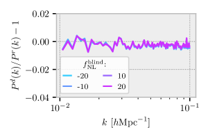
To recover the expected FKP field in Eq. 2.8, we have neglected the contribution of that does not appear in Eq. A.1. The difference between the two cases is negligible, as shown in the Figure 14 for the low-density subsample, where the difference is expected to be the highest.
To keep the definition of randoms as sampling the survey selection function141414Then randoms are the same for blind and non-blind data., with as little correlation as possible, we decided to apply the blinding weights to the data.
Appendix B Impact of blinding scheme on the quadrupole and hexadecapole
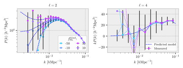
As described in Eq. 2.10, the blinding scheme is expected to modify the quadrupole (). However, the hexadecapole () in the linear regime is and does not depend on the bias such that the blinding procedure should not modify it.
The quadrupole and hexadecapole for multiple values of and for the high-density sample are displayed in Figure 15. We recover the expected behavior for both quadrupole and hexadecapole. Note that the statistical power at large scales for the hexadecapole is very weak and our measurements match well enough the expected theoretical prediction without PNG signal.
Appendix C Impact on the BAO / RSD measurement
As explained in Section 3.4, the window function related to the reconstruction prevents small scales from being impacted by the PNG blinding scheme. Hence, we quantify here the impact of this blinding scheme on the BAO/RSD measurement and how it can be incorporated with the BAO and the RSD blinding given in [35]. In this section, we are using the DESI blinding pipeline described in [45]151515https://github.com/desihub/LSS/blob/main/scripts/main/apply_blinding_main_fromfile_fcomp.py.
For this test, we used the 25 mock catalogs from the AbacasSummit N-body simulations [72, 73] that are transformed into light-cone to mimic the DESI DR1 Luminous Red Galaxy sample (LRG) [74] and use the full redshift range (). The associated covariance with this sample is produced by TheCov161616https://github.com/cosmodesi/thecov [75, 76, 77]. We use the monopole, quadrupole and hexadecapole for with a binning of .
We perform a standard full shape analysis using the 1-loop power spectrum computed by velocileptors171717https://github.com/sfschen/velocileptors [78, 79]. As usual, we parameterize the Alcock-Paczynski (AP) effect [80] with such that the power spectrum in the true cosmological coordinates is related to the power spectrum in observable coordinates by
| (C.1) |
with and the shifts along and perpendicular to the line-of-sight, respectively. We denote the value of in the fiducial cosmology used to transform redshift into distances. See, for instance, [81] for a complete description.
In addition to the AP parameters , we also fit the growth rate via and the ShapeFit parameter . The parameter is extracted thanks to the RSD terms. The ShapeFit parameter was introduced by [82] in order to collect additional information thanks to the shape of the power spectrum. It modifies the linear power spectrum as
| (C.2) |
where we use [82] and is the pivot scale. is the linear power spectrum of the fiducial theory that is fixed during all the fit.
We test several different blinding configurations based on two BAO/RSD blinding configurations181818See [45] for a description of the BAO/RSD blinding values.: blind-1 and blind-2 , for which we test a PNG blinding value of . For comparison, we also test, for the same PNG blinding value, a configuration without the BAO/RSD blinding.
The posteriors are drawn from the mean power spectrum of the 25 mocks to reduce the cosmic variance, but we use the covariance for the DR1 sample. They are obtained with emcee [83] and displayed in Figure 16. Note that we have a larger value of than expected due to wrong velocities for this version of simulation. This was corrected in the latter versions, however it will not impact the discussion here. Adding the PNG blinding appears to have no impact on the BAO/RSD parameters and slightly impacts the ShapeFit parameter , as already noticed with simulations with PNG signal [84] since the PNG blinding changes the large-scale slope of the power spectrum.
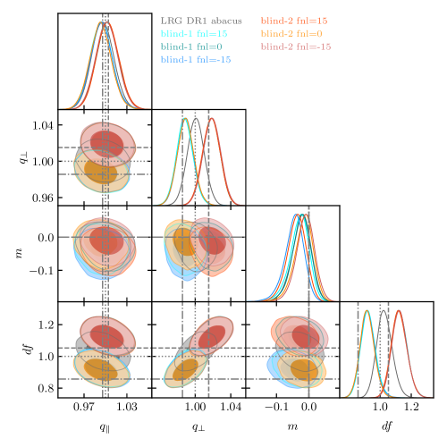
To quantify the deviation, the ratios between the parameters measured with the different blinded configurations and with the non-blinded case are plotted in Figure 17. The parameters are computed as the mean in the MCMC chains, while the errors are the credible interval from the chains in the blinded cases. The gray lines are the ratios between the expected value from the blinding and those measured in the non-blinded case.
We note that the PNG blinding scheme, as expected, does not impact the scales where the BAO and RSD parameters are measured and, therefore, can be included without biasing the further analysis of these measurements. The discrepancy on is expected, as explained in [84]. It is not a major issue however, as shifts remain below the statistical uncertainty, and the blinding procedure primarily aims at hiding and .

Appendix D Author Affiliations
1Lawrence Berkeley National Laboratory, 1 Cyclotron Road, Berkeley, CA 94720, USA
2IRFU, CEA, Université Paris-Saclay, F-91191 Gif-sur-Yvette, France
3Physics Dept., Boston University, 590 Commonwealth Avenue, Boston, MA 02215, USA
4Department of Physics & Astronomy, University College London, Gower Street, London, WC1E 6BT, UK
5Institute for Computational Cosmology, Department of Physics, Durham University, South Road, Durham DH1 3LE, UK
6Instituto de Física, Universidad Nacional Autónoma de México, Cd. de México C.P. 04510, México
7Kavli Institute for Particle Astrophysics and Cosmology, Stanford University, Menlo Park, CA 94305, USA
8SLAC National Accelerator Laboratory, Menlo Park, CA 94305, USA
9Institut d’Estudis Espacials de Catalunya (IEEC), 08034 Barcelona, Spain
10Institute of Cosmology and Gravitation, University of Portsmouth, Dennis Sciama Building, Portsmouth, PO1 3FX, UK
11Institute of Space Sciences, ICE-CSIC, Campus UAB, Carrer de Can Magrans s/n, 08913 Bellaterra, Barcelona, Spain
12School of Mathematics and Physics, University of Queensland, 4072, Australia
13Sorbonne Université, CNRS/IN2P3, Laboratoire de Physique Nucléaire et de Hautes Energies (LPNHE), FR-75005 Paris, France
14Departament de Física, Serra Húnter, Universitat Autònoma de Barcelona, 08193 Bellaterra (Barcelona), Spain
15Institut de Física d’Altes Energies (IFAE), The Barcelona Institute of Science and Technology, Campus UAB, 08193 Bellaterra Barcelona, Spain
16NSF NOIRLab, 950 N. Cherry Ave., Tucson, AZ 85719, USA
17Institució Catalana de Recerca i Estudis Avançats, Passeig de Lluís Companys, 23, 08010 Barcelona, Spain
18Departamento de Física, Universidad de Guanajuato - DCI, C.P. 37150, Leon, Guanajuato, México
19Instituto Avanzado de Cosmología A. C., San Marcos 11 - Atenas 202. Magdalena Contreras, 10720. Ciudad de México, México
20Department of Physics and Astronomy, University of Waterloo, 200 University Ave W, Waterloo, ON N2L 3G1, Canada
21Perimeter Institute for Theoretical Physics, 31 Caroline St. North, Waterloo, ON N2L 2Y5, Canada
22Waterloo Centre for Astrophysics, University of Waterloo, 200 University Ave W, Waterloo, ON N2L 3G1, Canada
23Instituto de Astrofísica de Andalucía (CSIC), Glorieta de la Astronomía, s/n, E-18008 Granada, Spain
24Center for Cosmology and AstroParticle Physics, The Ohio State University, 191 West Woodruff Avenue, Columbus, OH 43210, USA
25Department of Astronomy, The Ohio State University, 4055 McPherson Laboratory, 140 W 18th Avenue, Columbus, OH 43210, USA
26The Ohio State University, Columbus, 43210 OH, USA
27Department of Physics and Astronomy, Sejong University, Seoul, 143-747, Korea
28CIEMAT, Avenida Complutense 40, E-28040 Madrid, Spain
29Department of Physics, University of Michigan, Ann Arbor, MI 48109, USA
30University of Michigan, Ann Arbor, MI 48109, USA
31Department of Physics & Astronomy, Ohio University, Athens, OH 45701, USA
32National Astronomical Observatories, Chinese Academy of Sciences, A20 Datun Rd., Chaoyang District, Beijing, 100012, P.R. China