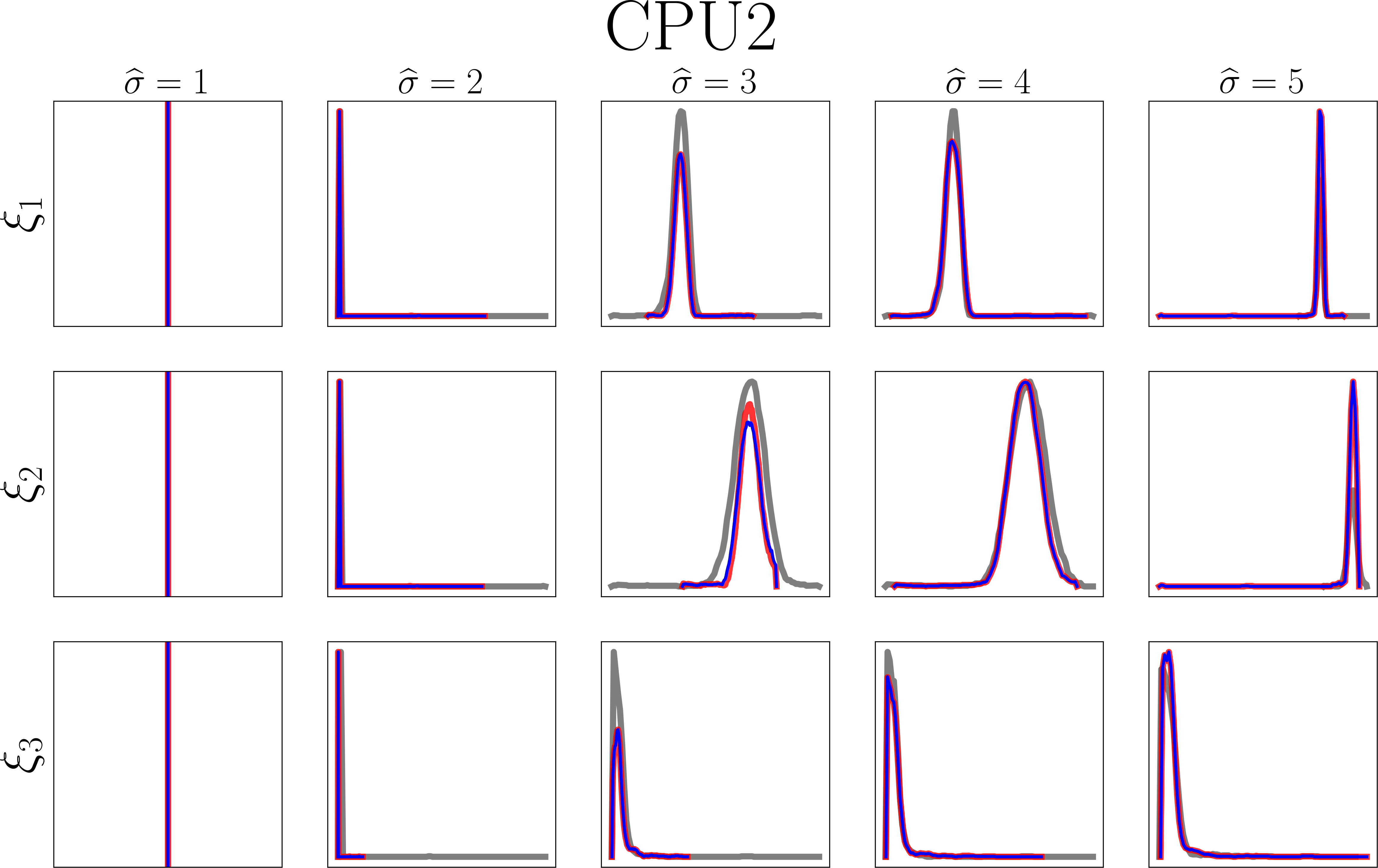
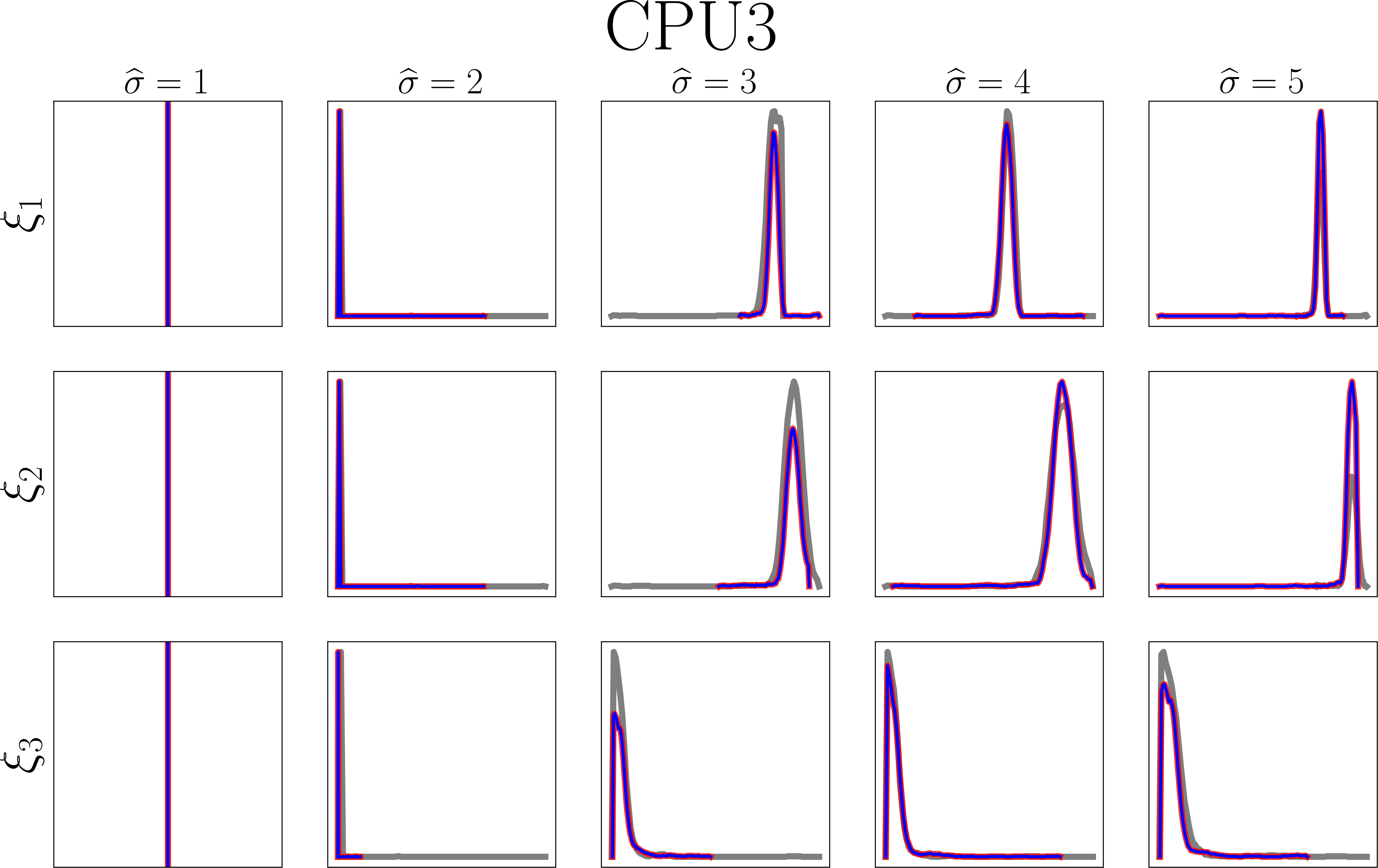
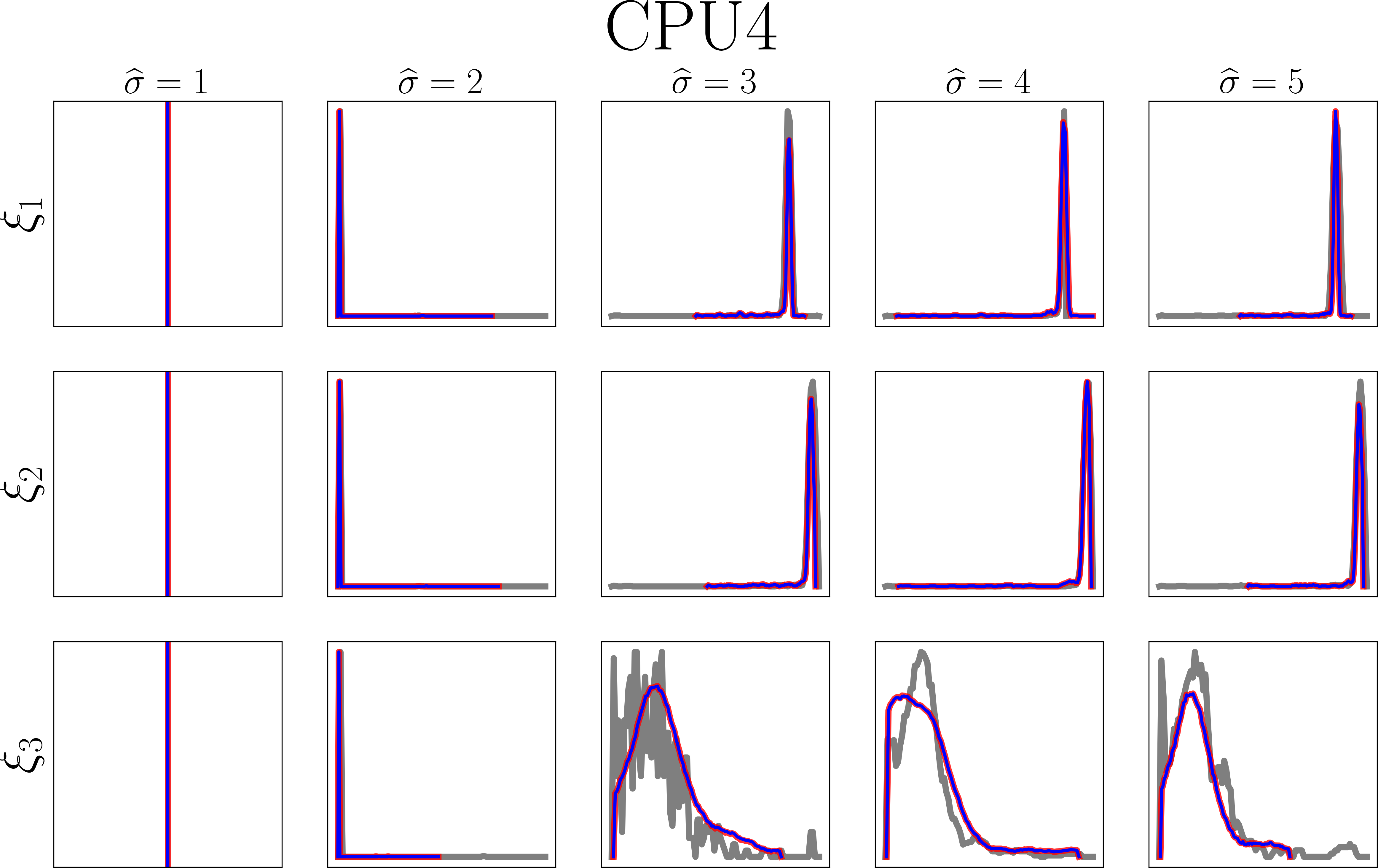
Stochastic Learning of Computational Resource Usage as
Graph Structured Multimarginal Schrödinger Bridge

Georgiy A. Bondar, Robert Gifford, Linh Thi Xuan Phan, Abhishek Halder Georgiy A. Bondar is with the Department of Applied Mathematics, University of California, Santa Cruz, CA 95064, USA, gbondar@ucsc.edu.Robert Gifford and Linh Thi Xuan Phan are with the Department of Computer and Information Science, University of Pennsylvania, Philadelphia, PA 19104, USA, {rgif,linhphan}@seas.upenn.edu.Abhishek Halder (corresponding author) is with the Department of Aerospace Engineering, Iowa State University, Ames, IA 50011, USA, ahalder@iastate.edu.This research was supported by NSF awards 2112755, 2111688 and 1750158.
Abstract

We propose to learn the time-varying stochastic computational resource usage of software as a graph structured Schrödinger bridge problem. In general, learning the computational resource usage from data is challenging because resources such as the number of CPU instructions and the number of last level cache requests are both time-varying and statistically correlated. Our proposed method enables learning the joint time-varying stochasticity in computational resource usage from the measured profile snapshots in a nonparametric manner. The method can be used to predict the most-likely time-varying distribution of computational resource availability at a desired time. We provide detailed algorithms for stochastic learning in both single and multi-core cases, discuss the convergence guarantees, computational complexities, and demonstrate their practical use in two case studies: a single-core nonlinear model predictive controller, and a synthetic multi-core software.

Keywords: Multimarginal Schrödinger bridge, stochastic learning, computational resource, multi-core hardware.

I Introduction

Compute-intensive software, including control software, often operate in hardware platforms that are different from where their performance were verified. This could be because of hardware up/downgrades in response to evolving project needs, technology progress and such. A natural question, then, is whether there could be a principled way to learn the stochastic dynamical nature of computational resource availability such as processor, memory bandwidth and last level shared cache (LLC). Such learning could then be leveraged to design dynamic scheduling algorithms by predicting, for example, the most likely joint computational resource that will be available at a future time. In this work, we propose such a stochastic learning framework for both single and multi-core platforms.

In the real-time systems community, it is well-known [1] that due to hardware-level stochasticity, multiple executions of the same software on the same hardware with identical initial conditions and parameters, result in different execution times. A common way to account for this is to analyze some lumped variable such as (worst-case or probabilistic) execution time [2, 3, 4] for a given software-hardware combination. In contrast, the ability to directly learn in the joint space of LLC, processor and memory availability, could enable the design of more fine-grained dynamic resource schedulers. This is of particular interest in safety-critical controlled cyber-physical systems that operate in resource-constrained environments because high performance controllers (e.g., MPC) are more compute-intensive and have more pronounced stochasticity than computationally benign controllers (e.g., PID).

Learning in the joint space, however, is technically challenging because variables such as processor availability, LLC and memory bandwidth are not only statistically correlated, but their correlations also change over time, i.e., they cannot be assumed as (neither strict nor wide-sense) stationary stochastic processes for learning purposes. It is also impractical to fit parametric statistical models such as a Markov chain by gridding the multi-dimensional space of computational resource state since the resource state space is not countable. In this work, we leverage the recent progress in multimarginal Schrödinger bridges to show the feasibility of nonparametric joint stochastic learning of computational resource usage from hardware-software profile data.

Related work

Multimarginal Schrödinger bridge problems (MSBPs) are entropy regularized variants of the multimarginal optimal mass transport (MOMT) problems [5, 6]. The latter has been applied to learning and inference problems in chemical physics [7, 8], team matching [9], fluid dynamics [10] and risk management [11]. For recent applications of MSBPs to learning and tracking problems, see e.g., [12, 13, 14]. The MSBPs can also be seen as generalized variants of the classical (a.k.a. bimarginal) Schrödinger bridge problems (SBPs) which we will explain in Sec. IV-A. In the control literature, there are growing works on the stochastic optimal control interpretations [15, 16], generalizations [17, 18, 19] and applications [20, 21, 22] of the SBPs.

Prior work has applied machine learning to performance prediction and workload modeling, especially in data center and cloud environments; see e.g., the surveys in [23, 24] and references therein. Unlike our work, these solutions focus on predicting coarse-grained characteristics – such as request rates, CPU utilization, memory and disk I/O usages, bandwidth, or energy consumption – and they do not consider the interdependent relationship among shared resources. In real-time and embedded systems, learning techniques have been used for estimating timing behaviors [25, 26, 27]; however, existing work focuses on the worst-case or probabilistic execution time of the entire software, rather than the dynamic resource usage patterns during an execution of the software. To our best knowledge, our work is the first to use learning for predicting the stochastic dynamical run-time behavior of computational resource usage that jointly considers interdependent resources on multi-core platforms (such as CPU, cache and memory bandwidth) as well as multi-threaded applications.

Contributions

This work builds on our preliminary work [28] but significantly extends the same by considering multi-core resources and more general graph structures than path tree. The specific contributions are threefold:

  • Mathematical formulations for the stochastic learning of computational resource usage as graph-structured MSBPs where the graph structures arise from single or multi-core computational platforms. These formulations are motivated by maximum likelihood interpretations in the path space.

  • Numerical algorithms for solving the proposed graph-stuctured MSBPs. We show that unlike generic graph structures, the MSBPs induced by single or multi-core computational resource usage lead to structured tensor optimization problems that can be leveraged to reduce the learning algorithms’ computational complexity from exponential to linear in number of observations.

  • Numerical experiments to illustrate the proposed learning framework. This includes a single-core MPC benchmark, and a synthetic multi-core software benchmark.

Organization

In Sec. II, we set up basic notations and background ideas to be used throughout this work. Sec. III outlines the overall problem formulation. Expanding on the same, Sec. IV explains the maximum likelihood interpretations motivating the ideas, and then gives mathematically precise formulations for single core (Sec. IV-C) and multi-core (Sec. IV-D, IV-E) CPU usages. Sec. V details the proposed algorithms and their computational complexities for solving the formulations in Sec. IV. In particular, algorithmic specifics for Sec. IV-C are in Sec. V-A, those for Sec. IV-D are in V-B, and those for Sec. IV-E are in Sec. V-C. Numerical experiments highlighting the efficacy of the proposed method are detailed in Sec. VI for both single and multi-core CPUs. Sec. VII concludes the paper. Proofs are given in the Appendix.

II Preliminaries

In this Section, we fix notations and background ideas that will be used subsequently.

Sets. For any natural number ν𝜈\nu, we use the finite set notation ν:={1,2,,ν}\llbracket\nu\rrbracket:=\{1,2,\ldots,\nu\}. We denote the cardinality of set 𝒮𝒮\mathcal{S} as |𝒮|𝒮|\mathcal{S}|. We will use the following.

Lemma 1.

[29, Thm. 19.2] Given finite sets 𝒮1𝒮2subscript𝒮1subscript𝒮2\mathcal{S}_{1}\subseteq\mathcal{S}_{2} with |𝒮1|=ν1subscript𝒮1subscript𝜈1|\mathcal{S}_{1}|=\nu_{1} and |𝒮2|=ν2subscript𝒮2subscript𝜈2|\mathcal{S}_{2}|=\nu_{2}, we have |𝒮2𝒮1|=ν2ν1subscript𝒮2subscript𝒮1subscript𝜈2subscript𝜈1|\mathcal{S}_{2}\setminus\mathcal{S}_{1}|=\nu_{2}-\nu_{1}.

Vectors, matrices, tensors. We use unboldfaced (resp. boldfaced) small letters to denote scalars (resp. vectors). Unboldfaced capital letters denote matrices and bold capital letters denote tensors of order three or more. We occasionally make exceptions for standard notations such as (2)-(3).

We use square braces to denote the components. For example, [𝑿i1,,ir]delimited-[]subscript𝑿subscript𝑖1subscript𝑖𝑟\left[\bm{X}_{i_{1},\ldots,i_{r}}\right] denotes the (i1,,ir)subscript𝑖1subscript𝑖𝑟(i_{1},\ldots,i_{r})th component of an order r𝑟r tensor 𝑿𝑿\bm{X}, where (i1,,ir)rsubscript𝑖1subscript𝑖𝑟superscript𝑟(i_{1},\ldots,i_{r})\in\mathbb{N}^{r}. We use the r𝑟r fold tensor product space notation (d)r:=ddrtimesassignsuperscriptsuperscript𝑑tensor-productabsent𝑟subscripttensor-productsuperscript𝑑superscript𝑑𝑟times\left(\mathbb{R}^{d}\right)^{\otimes r}:=\underbrace{\mathbb{R}^{d}\otimes\ldots\otimes\mathbb{R}^{d}}_{r\;\text{times}}.

For two given tensors 𝑿,𝒀𝑿𝒀\bm{X},\bm{Y} of order r𝑟r, their Hilbert-Schmidt inner product is

𝑿,𝒀:=i1,,ir[𝑿i1,,ir][𝒀i1,,ir].assign𝑿𝒀subscriptsubscript𝑖1subscript𝑖𝑟delimited-[]subscript𝑿subscript𝑖1subscript𝑖𝑟delimited-[]subscript𝒀subscript𝑖1subscript𝑖𝑟\displaystyle\langle\bm{X},\bm{Y}\rangle:=\sum_{i_{1},\ldots,i_{r}}\left[\bm{X}_{i_{1},\ldots,i_{r}}\right]\left[\bm{Y}_{i_{1},\ldots,i_{r}}\right]. (1)

The operators exp()\exp(\cdot), log()\log(\cdot), direct-product\odot and \oslash are all understood elementwise, i.e., denote elementwise exponential, logarithm, multiplication and division, respectively. Vector or matrix transposition is denoted by the superscript . We use diag(𝒗)diag𝒗{\rm{diag}}(\bm{v}) to denote a diagonal matrix with entries of vector 𝒗𝒗\bm{v} along its main diagonal, and 𝟏1\bm{1} to denote all ones column vector of suitable length.

Probability. A probability measure μ𝜇\mu over some Polish space 𝒳𝒳\mathcal{X} satisfies 𝒳dμ=1subscript𝒳differential-d𝜇1\int_{\mathcal{X}}{\rm{d}}\mu=1. For a pair of probability measures μ,ν𝜇𝜈\mu,\nu defined over two Polish spaces 𝒳,𝒴𝒳𝒴\mathcal{X},\mathcal{Y} respectively, their product measure is μνtensor-product𝜇𝜈\mu\otimes\nu, and 𝒳×𝒴d(μν)=1subscript𝒳𝒴dtensor-product𝜇𝜈1\int_{\mathcal{X}\times\mathcal{Y}}{\rm{d}}\left(\mu\otimes\nu\right)=1.

The entropy of a probability measure μ𝜇\mu is logμdμ𝜇d𝜇-\int\log\mu{\rm{d}}\mu. The relative entropy or Kullback-Leibler divergence DKL()D_{\rm{KL}}(\cdot\|\cdot) between two probability measures μ𝜇\mu and ν𝜈\nu is

DKL(μν):={logdμdνdμifμν,+otherwise,assignsubscript𝐷KLconditional𝜇𝜈casesd𝜇d𝜈d𝜇much-less-thanif𝜇𝜈otherwise,\displaystyle D_{\rm{KL}}(\mu\|\nu):=\begin{cases}\int\log\frac{{\rm{d}}\mu}{{\rm{d}}\nu}{\rm{d}}\mu&\text{if}\quad\mu\ll\nu,\\ +\infty&\text{otherwise,}\end{cases} (2)

where dμdνd𝜇d𝜈\frac{{\rm{d}}\mu}{{\rm{d}}\nu} denotes the Radon-Nikodym derivative, and μνmuch-less-than𝜇𝜈\mu\ll\nu is a shorthand for “μ𝜇\mu is absolutely continuous w.r.t. ν𝜈\nu”.

The Wasserstein distance W𝑊W between two probability measures μ,ν𝜇𝜈\mu,\nu, supported respectively on 𝒳,𝒴d𝒳𝒴superscript𝑑\mathcal{X},\mathcal{Y}\subseteq\mathbb{R}^{d}, is

W(μ,ν):=(infπΠ(μ,ν)𝒳×𝒴𝒙𝒚22dπ(𝒙,𝒚))12,assign𝑊𝜇𝜈superscript𝜋Π𝜇𝜈infimumsubscript𝒳𝒴superscriptsubscriptnorm𝒙𝒚22differential-d𝜋𝒙𝒚12\displaystyle W\left(\mu,\nu\right):=\left(\underset{\pi\in\Pi(\mu,\nu)}{\inf}\int_{\mathcal{X}\times\mathcal{Y}}\|\bm{x}-\bm{y}\|_{2}^{2}\>{\rm{d}}\pi(\bm{x},\bm{y})\right)^{\frac{1}{2}}, (3)

where the infimum in (3) is over all joint couplings of μ,ν𝜇𝜈\mu,\nu, i.e., Π(μ,ν):={probability measuresπ𝒴dπ=μ,𝒳dπ=ν}assignΠ𝜇𝜈conditional-setprobability measures𝜋formulae-sequencesubscript𝒴differential-d𝜋𝜇subscript𝒳differential-d𝜋𝜈\Pi(\mu,\nu):=\{\text{probability measures}\,\pi\mid\int_{\mathcal{Y}}{\rm{d}}\pi=\mu,\int_{\mathcal{X}}{\rm{d}}\pi=\nu\}. Unlike the Kullback-Leibler divergence (2), the Wasserstein distance (3) is a metric on the space of probability measures.

Hilbert projective metric. The Hilbert projective metric [30, 31, 32] dH(𝒖,𝒗)subscript𝑑H𝒖𝒗d_{\rm{H}}\left(\bm{u},\bm{v}\right) between 𝒖,𝒗>0n𝒖𝒗subscriptsuperscript𝑛absent0\bm{u},\bm{v}\in\mathbb{R}^{n}_{>0} (positive orthant) is

dH(𝒖,𝒗)=log(maxi=1,,nui/vimini=1,,nui/vi).subscript𝑑H𝒖𝒗subscript𝑖1𝑛subscript𝑢𝑖subscript𝑣𝑖subscript𝑖1𝑛subscript𝑢𝑖subscript𝑣𝑖\displaystyle d_{\rm{H}}\left(\bm{u},\bm{v}\right)=\log\left(\dfrac{\max_{i=1,\ldots,n}u_{i}/v_{i}}{\min_{i=1,\ldots,n}u_{i}/v_{i}}\right). (4)

The convergence plots w.r.t. Hilbert metric for our numerical experiments will be given in Sec. VI.

The formula (4) is a special case of the general definition of Hilbert metric dHsubscript𝑑Hd_{\rm{H}} between any two elements of a pointed***A cone 𝒦𝒦\mathcal{K} is pointed if 𝒦𝒦={0}\mathcal{K}\cap-\mathcal{K}=\{0\}. convex cone 𝒦𝒦\mathcal{K} in a real vector space:

dH(u,v)=log(inf{λ0λvu}sup{λ0uλv})u,v𝒦.formulae-sequencesubscript𝑑H𝑢𝑣infimumconditional-set𝜆0𝜆𝑣𝑢supremumconditional-set𝜆0𝑢𝜆𝑣for-all𝑢𝑣𝒦\displaystyle d_{\rm{H}}(u,v)=\log\left(\dfrac{\inf\{\lambda\geq 0\mid\lambda v\geq u\}}{\sup\{\lambda\geq 0\mid u\geq\lambda v\}}\right)\quad\forall u,v\in\mathcal{K}. (5)

Note that (5) reduces to (4) for 𝒦>0n𝒦subscriptsuperscript𝑛absent0\mathcal{K}\equiv\mathbb{R}^{n}_{>0}.

III Stochastic Learning of Computational Resource

We collect distributional data for the computational resource availability state thought of as a continuous-time stochastic process over time τ[0,t]𝜏0𝑡\tau\in[0,t]. In what follows, we will make these ideas precise. For now, let us begin by assuming that the data are collected at s,s2formulae-sequence𝑠𝑠2s\in\mathbb{N},s\geq 2 snapshots

τ10<τ2<<τs1<τst.subscript𝜏10subscript𝜏2subscript𝜏𝑠1subscript𝜏𝑠𝑡\displaystyle\tau_{1}\equiv 0<\tau_{2}<\ldots<\tau_{s-1}<\tau_{s}\equiv t. (6)

Define the snapshot index set s:={1,2,,s}\llbracket s\rrbracket:=\{1,2,\ldots,s\}.

We consider multi-core computing hardware with J𝐽J\in\mathbb{N} cores, and define the core index set J:={1,2,,J}\llbracket J\rrbracket:=\{1,2,\ldots,J\}. For jJj\in\llbracket J\rrbracket and for a given time horizon of interest [0,t]0𝑡[0,t], we think of the computational resource state vector 𝝃j(τ)superscript𝝃𝑗𝜏\bm{\xi}^{j}(\tau), 0τt0𝜏𝑡0\leq\tau\leq t, as a continuous time dsuperscript𝑑\mathbb{R}^{d}-valued stochastic process.

For each jJj\in\llbracket J\rrbracket, a (random) vectorial sample path 𝝃j(τ)superscript𝝃𝑗𝜏\bm{\xi}^{j}(\tau) is referred to as a profile. For the single core (J=1𝐽1J=1) case, we drop the core index superscript j𝑗j and simply denote the sample path or profile as 𝝃(τ)𝝃𝜏\bm{\xi}(\tau).

As a concrete example, consider the case 𝝃j3superscript𝝃𝑗superscript3\bm{\xi}^{j}\in\mathbb{R}^{3} jJ\forall j\in\llbracket J\rrbracket, with the components of 𝝃jsuperscript𝝃𝑗\bm{\xi}^{j} as

(ξ1jξ2jξ3j)=(instructions retiredLLC requestsLLC misses)jJ.\displaystyle\begin{pmatrix}\xi_{1}^{j}\\ \xi_{2}^{j}\\ \xi_{3}^{j}\end{pmatrix}=\begin{pmatrix}\text{instructions retired}\\ \text{LLC requests}\\ \text{LLC misses}\end{pmatrix}\>\forall j\in\llbracket J\rrbracket. (7)

In this example, the three elements of 𝝃jsuperscript𝝃𝑗\bm{\xi}^{j} denote the number of CPU instructions, the number of LLC requests, and the number of LLC misses in the last time unit (e.g., in the last 10 ms if the profiling frequency is 100 Hz), respectively, in the core jJj\in\llbracket J\rrbracket. We will use this specific 𝝃j3superscript𝝃𝑗superscript3\bm{\xi}^{j}\in\mathbb{R}^{3} in our numerical experiments (both single and multi-core). However, we will develop the proposed stochastic learning framework for generic 𝝃jdsuperscript𝝃𝑗superscript𝑑\bm{\xi}^{j}\in\mathbb{R}^{d}. This will allow generalizability in the sense that the proposed method can be adapted to an application at hand with a custom definition of the d𝑑d\in\mathbb{N} components of the stochastic state 𝝃jsuperscript𝝃𝑗\bm{\xi}^{j}.

Refer to caption
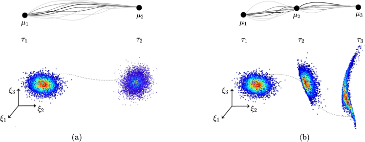
Figure 1: (a) The classical (bimarginal) SBP computes the most likely measure-valued curve connecting two given probability measures μ1,μ2subscript𝜇1subscript𝜇2\mu_{1},\mu_{2} at times τ1,τ2subscript𝜏1subscript𝜏2\tau_{1},\tau_{2} respectively. (b) The MSBP computes the most likely measure-valued curve connecting multiple, here three given probability measures μ1,μ2,μ3subscript𝜇1subscript𝜇2subscript𝜇3\mu_{1},\mu_{2},\mu_{3} at times τ1,τ2,τ3subscript𝜏1subscript𝜏2subscript𝜏3\tau_{1},\tau_{2},\tau_{3} respectively. In both subfigures, the feasible measured-valued curves are shown in the top with darker (resp. lighter) hues for higher (resp. lower) probability. The given measures are shown in the bottom as colored scatter plots (red = high probability, blue = low probability) in the ground coordinates (ξ1,ξ2,ξ3)3superscriptsubscript𝜉1subscript𝜉2subscript𝜉3topsuperscript3(\xi_{1},\xi_{2},\xi_{3})^{\top}\in\mathbb{R}^{3}.

The distributional (i.e., measure-valued) observations collected at instances (6) comprise a sequence of joint state probability distributions or measures {μσj}(j,σ)J×ssubscriptsuperscriptsubscript𝜇𝜎𝑗𝑗𝜎delimited-⟦⟧𝐽delimited-⟦⟧𝑠\{\mu_{\sigma}^{j}\}_{(j,\sigma)\in\llbracket J\rrbracket\times\llbracket s\rrbracket}, i.e.,

𝝃j(τσ)μσj,dμσj(𝝃j(τσ))=1(j,σ)J×s.\displaystyle\bm{\xi}^{j}\left(\tau_{\sigma}\right)\sim\mu_{\sigma}^{j},\int\mathrm{d}\mu_{\sigma}^{j}\left(\bm{\xi}^{j}\left(\tau_{\sigma}\right)\right)=1\quad\forall(j,\sigma)\in\llbracket J\rrbracket\times\llbracket s\rrbracket. (8)

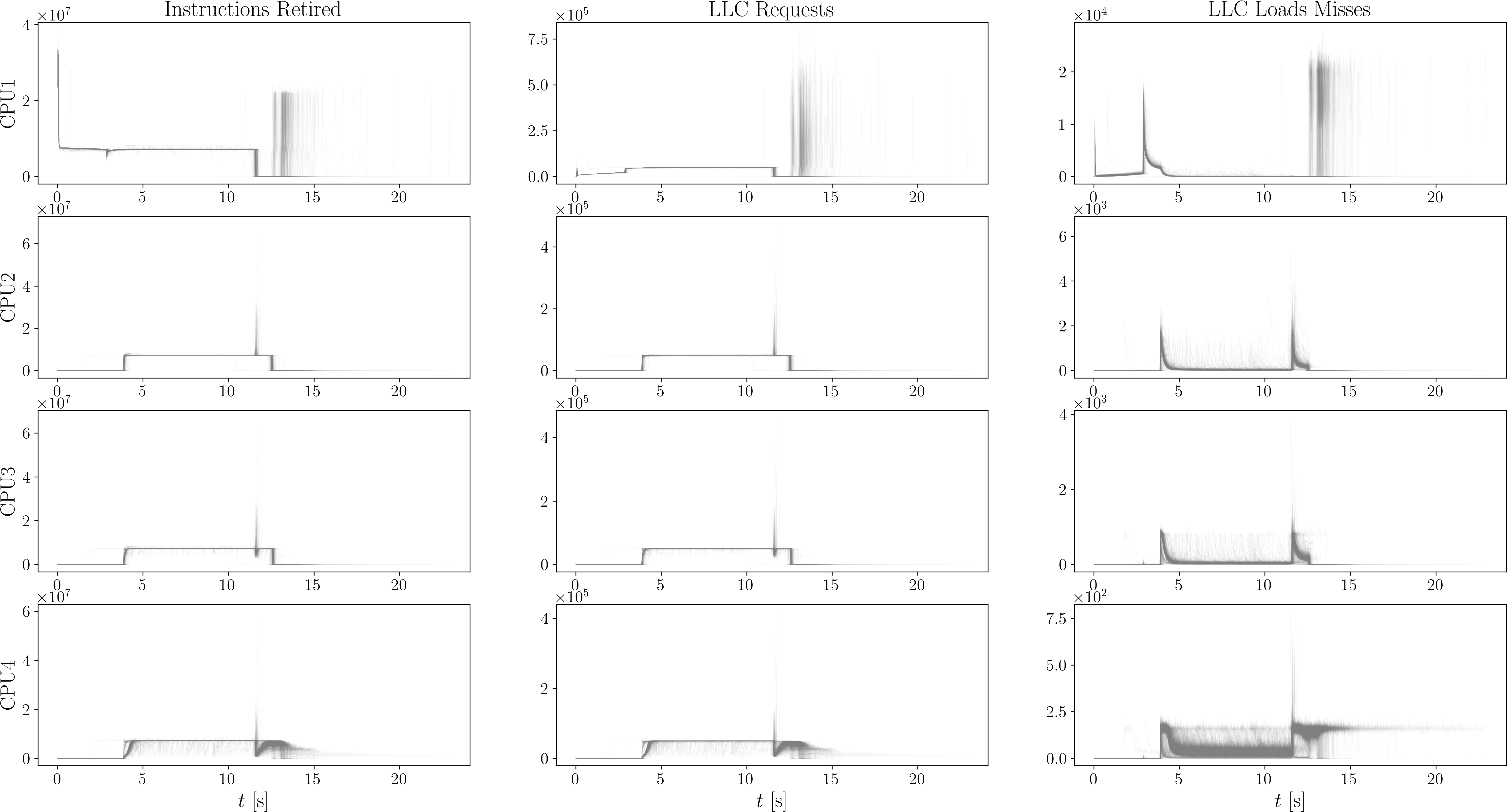
In this work, we are interested in learning the hardware-level stochasticity, i.e., the stochasticity in the state 𝝃jsuperscript𝝃𝑗\bm{\xi}^{j} arises from dynamic resource variability. In other words, repeated execution of the same (e.g., control) software with the same initial condition and same parameters result in different profiles 𝝃j(τ)superscript𝝃𝑗𝜏\bm{\xi}^{j}(\tau), (j,σ)J×s(j,\sigma)\in\llbracket J\rrbracket\times\llbracket s\rrbracket, 0τt0𝜏𝑡0\leq\tau\leq t. See Fig. 5 and Fig. 9 as exemplar single core and multi-core profiles, respectively.

Intuitively, when the hardware-level stochasticity is negligible, then the distributions μσjsuperscriptsubscript𝜇𝜎𝑗\mu_{\sigma}^{j} will be approximately Dirac deltas supported on the graph of a single path. When the stochastic variability is significant, μσjsuperscriptsubscript𝜇𝜎𝑗\mu_{\sigma}^{j} will have significant dispersion.

In practice, the probability measures {μσj}(j,σ)J×ssubscriptsuperscriptsubscript𝜇𝜎𝑗𝑗𝜎delimited-⟦⟧𝐽delimited-⟦⟧𝑠\{\mu_{\sigma}^{j}\}_{(j,\sigma)\in\llbracket J\rrbracket\times\llbracket s\rrbracket} are only available empirically from a fixed, say n𝑛n\in\mathbb{N} profiles. Let the sample or profile index ini\in\llbracket n\rrbracket. We accordingly set

μσj:=1ni=1nδ(𝝃j𝝃i,j(τσ))(j,σ)J×s\displaystyle\mu_{\sigma}^{j}:=\frac{1}{n}\sum_{i=1}^{n}\delta\left(\bm{\xi}^{j}-\bm{\xi}^{i,j}\left(\tau_{\sigma}\right)\right)\>\forall(j,\sigma)\in\llbracket J\rrbracket\times\llbracket s\rrbracket (9)

where δ(𝝃j𝝃i,j(τσ))𝛿superscript𝝃𝑗superscript𝝃𝑖𝑗subscript𝜏𝜎\delta\left(\bm{\xi}^{j}-\bm{\xi}^{i,j}\left(\tau_{\sigma}\right)\right) denotes the Dirac delta at the i𝑖ith sample location 𝝃i,j(τσ)dsuperscript𝝃𝑖𝑗subscript𝜏𝜎superscript𝑑\bm{\xi}^{i,j}\left(\tau_{\sigma}\right)\in\mathbb{R}^{d} for a fixed index pair (j,σ)J×s(j,\sigma)\in\llbracket J\rrbracket\times\llbracket s\rrbracket. For any fixed pair (j,σ)J×s(j,\sigma)\in\llbracket J\rrbracket\times\llbracket s\rrbracket, the finite set {𝝃i,j(τσ)}i=1nsuperscriptsubscriptsuperscript𝝃𝑖𝑗subscript𝜏𝜎𝑖1𝑛\{\bm{\xi}^{i,j}\left(\tau_{\sigma}\right)\}_{i=1}^{n} is a scattered point cloud.

With the basic notations in place, the informal statement for our stochastic learning problem is as follows.
Most likely distributional learning problem (informal). Given distributional snapshots (8), predict the most likely distribution of the computational resource state

𝝃j(τ)μτj,jJ,for anyτ[0,t].\displaystyle\bm{\xi}^{j}\left({\tau}\right)\sim\mu_{\tau}^{j},\;j\in\llbracket J\rrbracket,\;\text{for any}\>\tau\in[0,t]. (10)

In the next section, we will formalize this problem statement and discuss the related information graph structures.

IV MSBP and Graph Structures

To motivate the mathematical formulation, we start by outlining the classical (bimarginal) SBP in Sec. IV-A. Then in Sec. IV-B, we make the informal statement mentioned at the end of the previous Section rigorous using the framework of large deviation principle [33]. The resulting MSBP formulation takes the form of a maximum likelihood problem in the space of probability measure-valued curves, generalizing a similar formulation for the classical SBP.

We then consider specific cases of this MSBP formulation which result from the information graph structures induced by the stochastic profiles in single and multi-core computing hardware. In particular, Sec. IV-C details MSBP over a path tree which is the information graph structure that arises in the single core profiling. For the multi-core case, we discuss two different information graph structures in Sec. IV-D and IV-E.

IV-A Classical SBP and its Maximum Likelihood Iterpretation

In 1931-32, Erwin Schrödinger formulated what is now called the classical SBP, in two works: one written in German [34] and another in French [35]. For a relatively recent survey, see [36]. The classical SBP corresponds to the bimarginal (i.e., s=2𝑠2s=2) maximum likelihood problem: its solution finds the most likely measure-valued curve μτsubscript𝜇𝜏\mu_{\tau} where τ[0,t]𝜏0𝑡\tau\in[0,t] connecting the given endpoint measures μ1,μ2subscript𝜇1subscript𝜇2\mu_{1},\mu_{2} at τ1=0subscript𝜏10\tau_{1}=0 and τ2=tsubscript𝜏2𝑡\tau_{2}=t with respective supports over subsets of dsuperscript𝑑\mathbb{R}^{d}. See Fig. 1(a).

The classical SBP formulation proceeds as follows. Let 𝒳1,𝒳2dsubscript𝒳1subscript𝒳2superscript𝑑\mathcal{X}_{1},\mathcal{X}_{2}\subseteq\mathbb{R}^{d} be the supports of the given endpoint measures μ1,μ2subscript𝜇1subscript𝜇2\mu_{1},\mu_{2}, respectively. Letting 𝓧:=𝒳1×𝒳2d×dassign𝓧subscript𝒳1subscript𝒳2superscript𝑑superscript𝑑\bm{\mathcal{X}}:=\mathcal{X}_{1}\times\mathcal{X}_{2}\subseteq\mathbb{R}^{d}\times\mathbb{R}^{d}, we define a symmetric ground cost C:𝓧0:𝐶maps-to𝓧subscriptabsent0C:\bm{\mathcal{X}}\mapsto\mathbb{R}_{\geq 0}, i.e., C(𝝃(τ1),𝝃(τ2))𝐶𝝃subscript𝜏1𝝃subscript𝜏2C(\bm{\xi}(\tau_{1}),\bm{\xi}(\tau_{2})) is a distance between the random vectors 𝝃(τ1),𝝃(τ2)𝝃subscript𝜏1𝝃subscript𝜏2\bm{\xi}(\tau_{1}),\bm{\xi}(\tau_{2}). Let (𝓧)𝓧\mathcal{M}\left(\bm{\mathcal{X}}\right) denote the manifold of joint probability measures on the product space 𝓧𝓧\bm{\mathcal{X}}. For fixed but not necessarily small ε>0𝜀0\varepsilon>0, the classical SBP is an infinite dimensional convex problem:

min𝑴(𝓧)𝓧{C(𝝃(τ1),𝝃(τ2))+εlog𝑴(𝝃(τ1),𝝃(τ2))}𝑴𝓧subscript𝓧𝐶𝝃subscript𝜏1𝝃subscript𝜏2𝜀𝑴𝝃subscript𝜏1𝝃subscript𝜏2\displaystyle\underset{\bm{M}\in\mathcal{M}\left(\bm{\mathcal{X}}\right)}{\min}\!\int_{\bm{\mathcal{X}}}\!\big{\{}C\left(\bm{\xi}(\tau_{1}),\bm{\xi}(\tau_{2})\right)+\varepsilon\log\bm{M}\!\left(\bm{\xi}(\tau_{1}),\bm{\xi}(\tau_{2})\right)\!\!\big{\}}
d𝑴(𝝃(τ1),𝝃(τ2))d𝑴𝝃subscript𝜏1𝝃subscript𝜏2\displaystyle\qquad\qquad\qquad\qquad\qquad\qquad\qquad{\rm{d}}\bm{M}\!\left(\bm{\xi}(\tau_{1}),\bm{\xi}(\tau_{2})\right) (11a)
subject to𝒳2d𝑴(𝝃(τ1),𝝃(τ2))=μ1,subject tosubscriptsubscript𝒳2differential-d𝑴𝝃subscript𝜏1𝝃subscript𝜏2subscript𝜇1\displaystyle\text{subject to}\int_{\mathcal{X}_{2}}{\rm{d}}\bm{M}\!\left(\bm{\xi}(\tau_{1}),\bm{\xi}(\tau_{2})\right)=\mu_{1}, (11b)
𝒳1d𝑴(𝝃(τ1),𝝃(τ2))=μ2.subscriptsubscript𝒳1differential-d𝑴𝝃subscript𝜏1𝝃subscript𝜏2subscript𝜇2\displaystyle\qquad\qquad\int_{\mathcal{X}_{1}}{\rm{d}}\bm{M}\!\left(\bm{\xi}(\tau_{1}),\bm{\xi}(\tau_{2})\right)=\mu_{2}. (11c)

In words, (11) seeks to compute a joint probability measure that minimizes the entropy-regularized transportation cost (11a) subject to prescribed marginal constraints (11b)-(11c).

Notice that (𝓧)𝓧\mathcal{M}(\bm{\mathcal{X}}) is a convex set. The objective (11a) is strictly convex in 𝑴𝑴\bm{M}, thanks to the ε𝜀\varepsilon-regularized negative entropy term 𝓧εlog𝑴d𝑴subscript𝓧𝜀𝑴d𝑴\int_{\bm{\mathcal{X}}}\varepsilon\log\bm{M}\>{\rm{d}}\bm{M}. The constraints (11b)-(11c) are linear.

To clarify the maximum likelihood interpretation of (11), let 𝒞([τ1,τ2],d)𝒞subscript𝜏1subscript𝜏2superscript𝑑\mathcal{C}\left([\tau_{1},\tau_{2}],\mathbb{R}^{d}\right) denote the collection of continuous functions on the time interval [τ1,τ2]subscript𝜏1subscript𝜏2[\tau_{1},\tau_{2}] taking values in dsuperscript𝑑\mathbb{R}^{d}. Let Π(μ1,μ2)Πsubscript𝜇1subscript𝜇2\Pi(\mu_{1},\mu_{2}) be the collection of all path measures on 𝒞([τ1,τ2],d)𝒞subscript𝜏1subscript𝜏2superscript𝑑\mathcal{C}\left([\tau_{1},\tau_{2}],\mathbb{R}^{d}\right) with time τ1subscript𝜏1\tau_{1} marginal μ1subscript𝜇1\mu_{1}, and time τ2subscript𝜏2\tau_{2} marginal μ2subscript𝜇2\mu_{2}. Given a symmetric ground cost (e.g., Euclidean distance) C:𝒳1×𝒳20:𝐶maps-tosubscript𝒳1subscript𝒳2subscriptabsent0C:\mathcal{X}_{1}\times\mathcal{X}_{2}\mapsto\mathbb{R}_{\geq 0}, let

K(,):=exp(C(,)ε),assign𝐾𝐶𝜀\displaystyle K(\cdot,\cdot):=\exp\left(-\dfrac{C(\cdot,\cdot)}{\varepsilon}\right), (12)

and consider the bimarginal Gibbs kernel

K(𝝃(τ1),𝝃(τ2))μ1μ2.tensor-product𝐾𝝃subscript𝜏1𝝃subscript𝜏2subscript𝜇1subscript𝜇2\displaystyle K\left(\bm{\xi}(\tau_{1}),\bm{\xi}(\tau_{2})\right)\mu_{1}\otimes\mu_{2}. (13)

Recall that the minimizer of problem (11) is an optimal coupling 𝑴opt(𝓧)subscript𝑴opt𝓧\bm{M}_{\rm{opt}}\in\mathcal{M}\left(\bm{\mathcal{X}}\right). Proposition 1 next formalizes why the solution of (11) corresponds to the most likely measure-valued path (Fig. 1(a)) consistent with the observed measure-valued snapshots μ1,μ2subscript𝜇1subscript𝜇2\mu_{1},\mu_{2}. Its proof uses Sanov’s theorem [37]; for details we refer the readers to the references below.

Proposition 1.

([38, Sec. II],[39, Sec. 2.1]) The optimal coupling 𝐌opt(𝓧)subscript𝐌opt𝓧\bm{M}_{\rm{opt}}\in\mathcal{M}\left(\bm{\mathcal{X}}\right) in (11) corresponds to the optimal measure-valued path πoptΠ(μ1,μ2)subscript𝜋optΠsubscript𝜇1subscript𝜇2\pi_{\rm{opt}}\in\Pi(\mu_{1},\mu_{2}) solving the (scaled) relative entropy minimization problem:

minπΠ(μ1,μ2)εDKL(πK(𝝃(τ1),𝝃(τ2))μ1μ2).𝜋Πsubscript𝜇1subscript𝜇2𝜀subscript𝐷KLconditional𝜋tensor-product𝐾𝝃subscript𝜏1𝝃subscript𝜏2subscript𝜇1subscript𝜇2\displaystyle\underset{\pi\in\Pi(\mu_{1},\mu_{2})}{\min}\varepsilon D_{\rm{KL}}\left(\pi\|K\left(\bm{\xi}(\tau_{1}),\bm{\xi}(\tau_{2})\right)\mu_{1}\otimes\mu_{2}\right). (14)
Remark 1.

(Existence-uniqueness of the solution for (14)) Under the stated assumptions on the ground cost C𝐶C, the existence of minimizer for (14) is guaranteed [40, 41]. The uniqueness of the minimizer follows from strict convexity of the map πDKL(πν)maps-to𝜋subscript𝐷KLconditional𝜋𝜈\pi\mapsto D_{\rm{KL}}(\pi\|\nu) for fixed ν𝜈\nu.

Remark 2.

Intuitively, Proposition 1 links the solution of a static optimization problem (11) with that of a dynamic optimization problem (14) in the sense that the minimization in (14) is performed over all continuous measure-valued curves connecting the endpoints μ1,μ2subscript𝜇1subscript𝜇2\mu_{1},\mu_{2}.

Our setting in (10) requires generalizing these ideas for the multimarginal (s2𝑠2s\geq 2) case discussed next.

IV-B MSBP Formulation

In the single core (J=1)𝐽1(J=1) case, Fig. 1(b) illustrates how the MSBP of our interest generalizes the classical a.k.a. bimarginal SBP in Fig. 1(a).

In general, for any J𝐽J\in\mathbb{N}, we start by defining

𝒳σj:=support(μσj)d(j,σ)J×s,\displaystyle\mathcal{X}_{\sigma}^{j}:={\rm{support}}\left(\mu_{\sigma}^{j}\right)\subseteq\mathbb{R}^{d}\quad\forall(j,\sigma)\in\llbracket J\rrbracket\times\llbracket s\rrbracket, (15)

the Cartesian product

𝓧:=(j,σ)J×s𝒳σj(d)Js,assign𝓧subscriptproduct𝑗𝜎delimited-⟦⟧𝐽delimited-⟦⟧𝑠superscriptsubscript𝒳𝜎𝑗superscriptsuperscript𝑑tensor-productabsent𝐽𝑠\displaystyle\bm{\mathcal{X}}:=\prod_{(j,\sigma)\in\llbracket J\rrbracket\times\llbracket s\rrbracket}\mathcal{X}_{\sigma}^{j}\subseteq\left(\mathbb{R}^{d}\right)^{\otimes Js}, (16)

and a ground cost 𝑪:𝓧0:𝑪maps-to𝓧subscriptabsent0\bm{C}:\bm{\mathcal{X}}\mapsto\mathbb{R}_{\geq 0}.

Let (𝓧)𝓧\mathcal{M}\left(\bm{\mathcal{X}}\right) denote the manifold of probability measures on 𝓧𝓧\bm{\mathcal{X}}, and for a fixed pair (j,σ)J×s(j,\sigma)\in\llbracket J\rrbracket\times\llbracket s\rrbracket, let

𝓧(j,σ)subscript𝓧𝑗𝜎\displaystyle\bm{\mathcal{X}}_{(-j,-\sigma)} :=(a,b)J×s(j,σ)𝒳ba.assignabsentsubscriptproduct𝑎𝑏delimited-⟦⟧𝐽delimited-⟦⟧𝑠𝑗𝜎subscriptsuperscript𝒳𝑎𝑏\displaystyle:=\prod_{(a,b)\in\llbracket J\rrbracket\times\llbracket s\rrbracket\setminus(j,\sigma)}\mathcal{X}^{a}_{b}. (17)

For a fixed ε>0𝜀0\varepsilon>0, the multimarginal Schrödinger bridge problem (MSBP), generalizes the bimarginal problem (11) as

min𝑴(𝓧)𝓧{𝑪(𝝃1(τ1),,𝝃J(τs))\displaystyle\underset{\bm{M}\in\mathcal{M}\left(\bm{\mathcal{X}}\right)}{\min}\int_{\bm{\mathcal{X}}}\big{\{}\bm{C}\left(\bm{\xi}^{1}(\tau_{1}),\ldots,\bm{\xi}^{J}(\tau_{s})\right)
+εlog𝑴(𝝃1(τ1),,𝝃J(τs))}d𝑴(𝝃1(τ1),,𝝃J(τs))\displaystyle+\varepsilon\log\bm{M}\left(\bm{\xi}^{1}(\tau_{1}),\ldots,\bm{\xi}^{J}(\tau_{s})\right)\}{\rm{d}}\bm{M}\left(\bm{\xi}^{1}(\tau_{1}),\ldots,\bm{\xi}^{J}(\tau_{s})\right) (18a)
subject to𝓧(j,σ)d𝑴(𝝃1(τ1),,𝝃J(τs))=μσjsubject tosubscriptsubscript𝓧𝑗𝜎differential-d𝑴superscript𝝃1subscript𝜏1superscript𝝃𝐽subscript𝜏𝑠subscriptsuperscript𝜇𝑗𝜎\displaystyle\text{subject to}\int_{\bm{\mathcal{X}}_{(-j,-\sigma)}}{\rm{d}}\bm{M}\left(\bm{\xi}^{1}(\tau_{1}),\ldots,\bm{\xi}^{J}(\tau_{s})\right)=\mu^{j}_{\sigma}
(j,σ)J×s.\displaystyle\qquad\qquad\qquad\qquad\qquad\qquad\forall(j,\sigma)\in\llbracket J\rrbracket\times\llbracket s\rrbracket. (18b)

The maximum likelihood interpretation for the bimarginal problem given in Proposition 1 generalizes for MSBP (18) as stated next in Proposition 2. Similar to the case in Proposition 1, its proof is by direct computation and omitted.

Proposition 2.

Given the sets (15), (16), ground cost 𝐂:𝓧0:𝐂maps-to𝓧subscriptabsent0\bm{C}:\bm{\mathcal{X}}\mapsto\mathbb{R}_{\geq 0} and fixed ε>0𝜀0\varepsilon>0, define

𝑲(𝝃1(τ1),,𝝃J(τs)):=exp(𝑪(𝝃1(τ1),,𝝃J(τs))ε),assign𝑲superscript𝝃1subscript𝜏1superscript𝝃𝐽subscript𝜏𝑠𝑪superscript𝝃1subscript𝜏1superscript𝝃𝐽subscript𝜏𝑠𝜀\displaystyle\bm{K}\left(\bm{\xi}^{1}(\tau_{1}),\ldots,\bm{\xi}^{J}(\tau_{s})\right):=\exp\left(-\dfrac{\bm{C}\left(\bm{\xi}^{1}(\tau_{1}),\ldots,\bm{\xi}^{J}(\tau_{s})\right)}{\varepsilon}\right), (19)

and the multimarginal Gibbs kernel

𝑲(𝝃1(τ1),,𝝃J(τs))μ11μsJ.tensor-product𝑲superscript𝝃1subscript𝜏1superscript𝝃𝐽subscript𝜏𝑠superscriptsubscript𝜇11subscriptsuperscript𝜇𝐽𝑠\displaystyle\bm{K}\left(\bm{\xi}^{1}\left(\tau_{1}\right),\ldots,\bm{\xi}^{J}\left(\tau_{s}\right)\right)\mu_{1}^{1}\otimes\ldots\otimes\mu^{J}_{s}. (20)

Let Π(μ11,,μsJ)Πsubscriptsuperscript𝜇11superscriptsubscript𝜇𝑠𝐽\Pi\left(\mu^{1}_{1},\ldots,\mu_{s}^{J}\right) denote the collection of measure-valued paths on 𝒞([τ1,τs],d)𝒞subscript𝜏1subscript𝜏𝑠superscript𝑑\mathcal{C}\left([\tau_{1},\tau_{s}],\mathbb{R}^{d}\right) with (j,σ)𝑗𝜎(j,\sigma) marginal μσjsuperscriptsubscript𝜇𝜎𝑗\mu_{\sigma}^{j} (j,σ)J×s\forall(j,\sigma)\in\llbracket J\rrbracket\times\llbracket s\rrbracket. Then the optimal coupling 𝐌opt(𝓧)subscript𝐌opt𝓧\bm{M}_{\rm{opt}}\in\mathcal{M}\left(\bm{\mathcal{X}}\right) in (18) corresponds to the optimal measure-valued path πoptΠ(μ11,,μsJ)subscript𝜋optΠsubscriptsuperscript𝜇11superscriptsubscript𝜇𝑠𝐽\pi_{\rm{opt}}\in\Pi\left(\mu^{1}_{1},\ldots,\mu_{s}^{J}\right) solving the (scaled) relative entropy minimization problem:

minπΠ(μ11,,μsJ)εDKL(π𝑲(𝝃1(τ1),,𝝃J(τs))μ11μsJ).𝜋Πsubscriptsuperscript𝜇11superscriptsubscript𝜇𝑠𝐽𝜀subscript𝐷KLconditional𝜋tensor-product𝑲superscript𝝃1subscript𝜏1superscript𝝃𝐽subscript𝜏𝑠subscriptsuperscript𝜇11subscriptsuperscript𝜇𝐽𝑠\displaystyle\underset{\pi\in\Pi(\mu^{1}_{1},\ldots,\mu_{s}^{J})}{\min}\varepsilon D_{\rm{KL}}\left(\pi\|\bm{K}\left(\bm{\xi}^{1}(\tau_{1}),\ldots,\bm{\xi}^{J}(\tau_{s})\right)\mu^{1}_{1}\otimes\ldots\otimes\mu^{J}_{s}\right). (21)

The existence-uniqueness of the minimizer for (21), and thus for (18), follows from the same strict convexity argument as in Remark 1.

Motivated by the maximum likelihood interpretation (21) for (18), we propose to solve (18) for learning the stochastic computational resource state (10). The minimizer of (18), 𝑴opt(𝝃1(τ1),,𝝃J(τs))superscript𝑴optsuperscript𝝃1subscript𝜏1superscript𝝃𝐽subscript𝜏𝑠\bm{M}^{\rm{opt}}\left(\bm{\xi}^{1}(\tau_{1}),\ldots,\bm{\xi}^{J}(\tau_{s})\right) can be used to compute the optimal bimarginal probability mass transport plans between any (j1,σ1),(j2,σ2)J×s(j_{1},\sigma_{1}),(j_{2},\sigma_{2})\in\llbracket J\rrbracket\times\llbracket s\rrbracket, expressed as the bimarginal analogue of (18b):

𝓧(j1,j2,σ1,σ2)d𝑴opt(𝝃1(τ1),,𝝃J(τs))subscriptsubscript𝓧subscript𝑗1subscript𝑗2subscript𝜎1subscript𝜎2differential-dsuperscript𝑴optsuperscript𝝃1subscript𝜏1superscript𝝃𝐽subscript𝜏𝑠\int_{\bm{\mathcal{X}}_{(-j_{1},-j_{2},-\sigma_{1},-\sigma_{2})}}{\rm{d}}\bm{M}^{\rm{opt}}\left(\bm{\xi}^{1}(\tau_{1}),\ldots,\bm{\xi}^{J}(\tau_{s})\right) (22)

where

𝓧(j1,j2,σ1,σ2):=(a,b)J×s{(j1,σ1)(j2,σ2)}𝒳ba.assignsubscript𝓧subscript𝑗1subscript𝑗2subscript𝜎1subscript𝜎2subscriptproduct𝑎𝑏delimited-⟦⟧𝐽delimited-⟦⟧𝑠subscript𝑗1subscript𝜎1subscript𝑗2subscript𝜎2subscriptsuperscript𝒳𝑎𝑏\bm{\mathcal{X}}_{(-j_{1},-j_{2},-\sigma_{1},-\sigma_{2})}:=\prod_{(a,b)\in\llbracket J\rrbracket\times\llbracket s\rrbracket\setminus\{(j_{1},\sigma_{1})\cup(j_{2},\sigma_{2})\}}\mathcal{X}^{a}_{b}.

The coupling (22) will find use in implementing our multimarginal Sinkhorn recursions in Sec. V.

We next discuss the discrete formulations of (18) that arise from the information graph structures in single and multi-core computing hardware for finite scattered data {𝝃i,j(τσ)}i=1nsuperscriptsubscriptsuperscript𝝃𝑖𝑗subscript𝜏𝜎𝑖1𝑛\{\bm{\xi}^{i,j}(\tau_{\sigma})\}_{i=1}^{n} and {μσj}(j,σ)J×ssubscriptsuperscriptsubscript𝜇𝜎𝑗𝑗𝜎delimited-⟦⟧𝐽delimited-⟦⟧𝑠\{\mu_{\sigma}^{j}\}_{(j,\sigma)\in\llbracket J\rrbracket\times\llbracket s\rrbracket} as in (9). We will see that the corresponding formulations lead to strictly convex problems over finite dimensional nonnegative tensors. To reduce the notational overload, we use the same boldfaced symbols for the continuous and discrete version of the tensors.

IV-C Path Structured MSBP

Refer to caption
Figure 2: The path tree for sequentially observed {μσ}σssubscriptsubscript𝜇𝜎𝜎delimited-⟦⟧𝑠\{\mu_{\sigma}\}_{\sigma\in\llbracket s\rrbracket}.

For single core (J=1𝐽1J=1) computing hardware, the stochastic process 𝝃(τ)𝝃𝜏\bm{\xi}(\tau) is indexed only by time τ[0,t]𝜏0𝑡\tau\in[0,t]. So the information graph structure is also induced by time, i.e., by sequential in time measure-valued observations {μσ}σssubscriptsubscript𝜇𝜎𝜎delimited-⟦⟧𝑠\{\mu_{\sigma}\}_{\sigma\in\llbracket s\rrbracket}. In other words, the information graph in this case is a path tree shown in Fig. 2. We refer to an MSBP specialized to such path tree as the path structured MSBP.

Thanks to the path tree structure, the ground cost 𝑪𝑪\bm{C} in this case can be written as

𝑪(𝝃(τ1),,𝝃(τs))=σ=1s1cσ(𝝃(τσ),𝝃(τσ+1))𝑪𝝃subscript𝜏1𝝃subscript𝜏𝑠superscriptsubscript𝜎1𝑠1subscript𝑐𝜎𝝃subscript𝜏𝜎𝝃subscript𝜏𝜎1\displaystyle\bm{C}\!\left(\bm{\xi}(\tau_{1}),\ldots,\bm{\xi}(\tau_{s})\right)=\sum_{\sigma=1}^{s-1}c_{\sigma}\left(\bm{\xi}(\tau_{\sigma}),\bm{\xi}(\tau_{\sigma+1})\right) (23)

where we choose the squared Euclidean distance sequential cost between two consecutive snapshot indices, i.e., cσ(,):=22c_{\sigma}(\cdot,\cdot):=\|\cdot-\cdot\|_{2}^{2} σs\forall\sigma\in\llbracket s\rrbracket.

To formulate the discrete version of the corresponding MSBP, notice that the ground cost in (18a), in general, is an order s𝑠s tensor 𝑪(n)0s𝑪subscriptsuperscriptsuperscript𝑛tensor-productabsent𝑠absent0\bm{C}\in\left(\mathbb{R}^{n}\right)^{\otimes s}_{\geq 0} having components

[𝑪i1,,is]=𝑪(𝝃i1,,𝝃is)delimited-[]subscript𝑪subscript𝑖1subscript𝑖𝑠𝑪subscript𝝃subscript𝑖1subscript𝝃subscript𝑖𝑠\displaystyle\left[\bm{C}_{i_{1},\ldots,i_{s}}\right]=\bm{C}\left(\bm{\xi}_{i_{1}},\ldots,\bm{\xi}_{i_{s}}\right) (24)

that encodes the cost of transporting unit amount of mass for an s𝑠s tuple (i1,,is)subscript𝑖1subscript𝑖𝑠(i_{1},\ldots,i_{s}). However, the path structured cost (23) implies that the s𝑠s tuple in (24) equals to σ=1s1cσ(𝝃iσ,𝝃iσ+1)superscriptsubscript𝜎1𝑠1subscript𝑐𝜎subscript𝝃subscript𝑖𝜎subscript𝝃subscript𝑖𝜎1\sum_{\sigma=1}^{s-1}c_{\sigma}\left(\bm{\xi}_{i_{\sigma}},\bm{\xi}_{i_{\sigma+1}}\right), which is a sum of suitable elements of s1𝑠1s-1 different (in our case, Euclidean) distance matrices.

The discrete mass tensor 𝑴(n)0s𝑴subscriptsuperscriptsuperscript𝑛tensor-productabsent𝑠absent0\bm{M}\in\left(\mathbb{R}^{n}\right)^{\otimes s}_{\geq 0} has components

[𝑴i1,,is]=𝑴(𝝃i1,,𝝃is),delimited-[]subscript𝑴subscript𝑖1subscript𝑖𝑠𝑴subscript𝝃subscript𝑖1subscript𝝃subscript𝑖𝑠\displaystyle\left[\bm{M}_{i_{1},\ldots,i_{s}}\right]=\bm{M}\left(\bm{\xi}_{i_{1}},\ldots,\bm{\xi}_{i_{s}}\right), (25)

where [𝑴i1,,is]delimited-[]subscript𝑴subscript𝑖1subscript𝑖𝑠\left[\bm{M}_{i_{1},\ldots,i_{s}}\right] denotes the amount of transported mass for an s𝑠s tuple (i1,,is)subscript𝑖1subscript𝑖𝑠(i_{1},\ldots,i_{s}).

Furthermore, for path structured MSBP, we can drop the core index superscript j𝑗j to simplify constraints (18b) as

𝓧σd𝑴(𝝃(τ1),,𝝃(τs))=μσσs.\displaystyle\int_{\bm{\mathcal{X}}_{-\sigma}}{\rm{d}}\bm{M}\left(\bm{\xi}(\tau_{1}),\ldots,\bm{\xi}(\tau_{s})\right)=\mu_{\sigma}\quad\forall\sigma\in\llbracket s\rrbracket. (26)

In the discrete version, the empirical marginals 𝝁σ0nsubscript𝝁𝜎subscriptsuperscript𝑛absent0\bm{\mu}_{\sigma}\in\mathbb{R}^{n}_{\geq 0} are supported on the finite sets {𝝃i(τσ)}i=1nsuperscriptsubscriptsuperscript𝝃𝑖subscript𝜏𝜎𝑖1𝑛\{\bm{\xi}^{i}(\tau_{\sigma})\}_{i=1}^{n} σs\forall\sigma\in\llbracket s\rrbracket. Then, the LHS of the constraints (26) are projections of the mass tensor (25) on the σ𝜎\sigmath marginal 𝝁σsubscript𝝁𝜎\bm{\mu}_{\sigma} σs\forall\sigma\in\llbracket s\rrbracket. We denote this projection as projσ(𝑴)subscriptproj𝜎𝑴\operatorname*{proj}_{\sigma}(\bm{M}), which is a mapping projσ:(n)0s0n:subscriptproj𝜎maps-tosubscriptsuperscriptsuperscript𝑛tensor-productabsent𝑠absent0subscriptsuperscript𝑛absent0\operatorname*{proj}_{\sigma}:\left(\mathbb{R}^{n}\right)^{\otimes s}_{\geq 0}\mapsto\mathbb{R}^{n}_{\geq 0}, and is given componentwise as

[projσ(𝑴)r]=i1,,iσ1,iσ+1,,is𝑴i1,,iσ1,r,iσ+1,,is.delimited-[]subscriptproj𝜎subscript𝑴𝑟subscriptsubscript𝑖1subscript𝑖𝜎1subscript𝑖𝜎1subscript𝑖𝑠subscript𝑴subscript𝑖1subscript𝑖𝜎1𝑟subscript𝑖𝜎1subscript𝑖𝑠\displaystyle\Big{[}{\rm{proj}}_{\sigma}\!\left(\bm{M}\right)_{r}\!\Big{]}\!\!=\!\!\!\!\sum_{i_{1},\ldots,i_{\sigma-1},i_{\sigma+1},\ldots,i_{s}}\!\!\!\!\!\!\!\!\bm{M}_{i_{1},\ldots,i_{\sigma-1},r,i_{\sigma+1},\ldots,i_{s}}. (27)

Similarly, the discrete version of (22) in the path structured case, is the projection of 𝑴(n)0s𝑴subscriptsuperscriptsuperscript𝑛tensor-productabsent𝑠absent0\bm{M}\in\left(\mathbb{R}^{n}\right)^{\otimes s}_{\geq 0} on the (σ1,σ2)subscript𝜎1subscript𝜎2(\sigma_{1},\sigma_{2})th marginal denoted as projσ1,σ2(𝑴)subscriptprojsubscript𝜎1subscript𝜎2𝑴\operatorname*{proj}_{\sigma_{1},\sigma_{2}}(\bm{M}), i.e., projσ1,σ2:(n)0s0n×n:subscriptprojsubscript𝜎1subscript𝜎2maps-tosubscriptsuperscriptsuperscript𝑛tensor-productabsent𝑠absent0subscriptsuperscript𝑛𝑛absent0\operatorname*{proj}_{\sigma_{1},\sigma_{2}}:\left(\mathbb{R}^{n}\right)^{\otimes s}_{\geq 0}\mapsto\mathbb{R}^{n\times n}_{\geq 0}, and is given componentwise as

[projσ1,σ2(𝑴)r,]delimited-[]subscriptprojsubscript𝜎1subscript𝜎2subscript𝑴𝑟\displaystyle\left[{\rm{proj}}_{\sigma_{1},\sigma_{2}}\!\left(\bm{M}\right)_{r,\ell}\!\right]
=iσσs{σ1,σ2}𝑴i1,,iσ11,r,iσ1+1,,iσ21,,iσ2+1,,is.absentsubscriptconditionalsubscript𝑖𝜎𝜎delimited-⟦⟧𝑠subscript𝜎1subscript𝜎2subscript𝑴subscript𝑖1subscript𝑖subscript𝜎11𝑟subscript𝑖subscript𝜎11subscript𝑖subscript𝜎21subscript𝑖subscript𝜎21subscript𝑖𝑠\displaystyle=\!\!\!\!\sum_{i_{\sigma}\mid\sigma\in\llbracket s\rrbracket\setminus\{\sigma_{1},\sigma_{2}\}}\!\!\!\!\!\!\!\!\bm{M}_{i_{1},\ldots,i_{\sigma_{1}-1},r,i_{\sigma_{1}+1},\ldots,i_{\sigma_{2}-1},\ell,i_{\sigma_{2}+1},\ldots,i_{s}}. (28)

Then, the discrete path structured version of (18) becomes

min𝑴(n)0s𝑪+εlog𝑴,𝑴𝑴subscriptsuperscriptsuperscript𝑛tensor-productabsent𝑠absent0𝑪𝜀𝑴𝑴\displaystyle\underset{\bm{M}\in\left(\mathbb{R}^{n}\right)^{\otimes s}_{\geq 0}}{\min}~{}\langle\bm{C}+\varepsilon\log\bm{M},\bm{M}\rangle (29a)
subject toprojσ(𝑴)=𝝁σσs.\displaystyle\text{subject to}~{}~{}{\rm{proj}}_{\sigma}\left(\bm{M}\right)=\bm{\mu}_{\sigma}\quad\forall\sigma\in\llbracket s\rrbracket. (29b)

Notice that (29) is a strictly convex problem in nssuperscript𝑛𝑠n^{s} decision variables, and is computationally intractable in general. In Sec. V, we will design algorithms to solve them efficiently.

IV-D Barycentric MSBP
Refer to caption
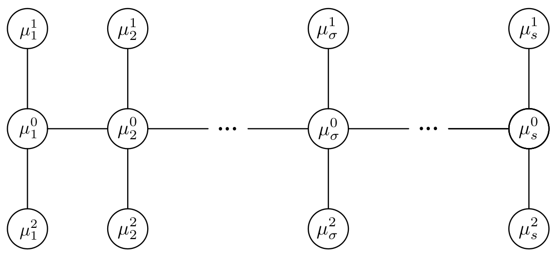
Figure 3: The tree graph for barycentric MSBP (Sec. IV-D) with measures {μσj}(j,σ)({0}J)×s\{\mu_{\sigma}^{j}\}_{(j,\sigma)\in\left(\{0\}\cup\llbracket J\rrbracket\right)\times\llbracket s\rrbracket}, where J=2𝐽2J=2.

For multi-core (J>1𝐽1J>1) computing hardware, the stochastic process 𝝃j(τ)superscript𝝃𝑗𝜏\bm{\xi}^{j}(\tau) is indexed by both time τ[0,t]𝜏0𝑡\tau\in[0,t] and CPU core jJj\in\llbracket J\rrbracket. Thus, the information graph structure is induced jointly by time and cores, i.e., by measure-valued observations {μσj}(j,σ)J×ssubscriptsuperscriptsubscript𝜇𝜎𝑗𝑗𝜎delimited-⟦⟧𝐽delimited-⟦⟧𝑠\{\mu_{\sigma}^{j}\}_{(j,\sigma)\in\llbracket J\rrbracket\times\llbracket s\rrbracket}. Unlike Sec. IV-C, we now have J𝐽J measure-valued snapshots at each time index. To account for this, we propose two different MSBP formulations, the first of which termed barycentric MSBP is discussed next.

The main idea behind our proposed barycentric MSBP formulation is to imagine a phantom CPU core whose statistics is the average (i.e., barycenter) of the measure-valued snapshots for all cores at any fixed time index σs\sigma\in\llbracket s\rrbracket. Accordingly, in this formulation, we consider the core index j{0}Jj\in\{0\}\cup\llbracket J\rrbracket where j=0𝑗0j=0 refers to the phantom barycentric CPU. The corresponding graph structure for J=2𝐽2J=2 is shown in Fig. 3. While a barycentric graph as in Fig. 3 is more general than the path tree as in Fig. 2, we note that the treewidth [42, p. 354-355] for barycentric graphs equals unity as in the path tree case. It is known that the computational complexity for graph-structured MSBP problems grow with the treewidth [43, 44]. We will discuss the specific complexity for the proposed algorithms in Sec. V.

The barycentric graph structure implies that (24) is no longer equal to σ=1s1cσ(𝝃iσ,𝝃iσ+1)superscriptsubscript𝜎1𝑠1subscript𝑐𝜎subscript𝝃subscript𝑖𝜎subscript𝝃subscript𝑖𝜎1\sum_{\sigma=1}^{s-1}c_{\sigma}\left(\bm{\xi}_{i_{\sigma}},\bm{\xi}_{i_{\sigma+1}}\right) as in Sec. IV-C, but instead becomes a sum of two types of ground transport costs, viz. the cost of transport between consecutive-in-time barycenters and the cost of transport between barycentric and actual CPU cores. Denoting the barycentric random vectors as {𝝃0(τσ)}σssubscriptsuperscript𝝃0subscript𝜏𝜎𝜎delimited-⟦⟧𝑠\{\bm{\xi}^{0}(\tau_{\sigma})\}_{\sigma\in\llbracket s\rrbracket}, and letting cj,σ(,)subscript𝑐𝑗𝜎c_{j,\sigma}(\cdot,\cdot) be the corresponding ground transport costs for all j{0}×Jj\in\{0\}\times\llbracket J\rrbracket, the cost (24) for barycentric MSBP equals

σ=1s1c0,σ(𝝃iσ0,𝝃iσ+10)+σ=1sj=1Jcj,σ(𝝃iσj,𝝃iσ0).superscriptsubscript𝜎1𝑠1subscript𝑐0𝜎superscriptsubscript𝝃subscript𝑖𝜎0subscriptsuperscript𝝃0subscript𝑖𝜎1superscriptsubscript𝜎1𝑠superscriptsubscript𝑗1𝐽subscript𝑐𝑗𝜎subscriptsuperscript𝝃𝑗subscript𝑖𝜎subscriptsuperscript𝝃0subscript𝑖𝜎\sum_{\sigma=1}^{s-1}c_{0,\sigma}\left(\bm{\xi}_{i_{\sigma}}^{0},\bm{\xi}^{0}_{i_{\sigma+1}}\right)+\sum_{\sigma=1}^{s}\sum_{j=1}^{J}c_{j,\sigma}\left(\bm{\xi}^{j}_{i_{\sigma}},\bm{\xi}^{0}_{i_{\sigma}}\right).

Similar ideas appeared in [12, Sec. 3.3] in a different context.

Defining the barycentric index set

ΛBC:=({0}J)×s,\displaystyle\Lambda_{\rm{BC}}:=(\{0\}\cup\llbracket J\rrbracket)\times\llbracket s\rrbracket, (30)

we note that |ΛBC|=(J+1)ssubscriptΛBC𝐽1𝑠|\Lambda_{\rm{BC}}|=(J+1)s, and thus for the barycentric MSBP, the tensors 𝑪,𝑴(n)0(J+1)s𝑪𝑴subscriptsuperscriptsuperscript𝑛tensor-productabsent𝐽1𝑠absent0\bm{C},\bm{M}\in\left(\mathbb{R}^{n}\right)^{\otimes(J+1)s}_{\geq 0}. In summary, the proposed barycentric MSBP is

min𝑴(n)0(J+1)s𝑪+εlog𝑴,𝑴𝑴subscriptsuperscriptsuperscript𝑛tensor-productabsent𝐽1𝑠absent0𝑪𝜀𝑴𝑴\displaystyle\underset{\bm{M}\in\left(\mathbb{R}^{n}\right)^{\otimes(J+1)s}_{\geq 0}}{\min}~{}\langle\bm{C}+\varepsilon\log\bm{M},\bm{M}\rangle (31a)
subject toproj(j,σ)(𝑴)=𝝁σj(j,σ)ΛBC.formulae-sequencesubject tosubscriptproj𝑗𝜎𝑴superscriptsubscript𝝁𝜎𝑗for-all𝑗𝜎subscriptΛBC\displaystyle\text{subject to}~{}~{}{\rm{proj}}_{(j,\sigma)}\left(\bm{M}\right)=\bm{\mu}_{\sigma}^{j}\quad\forall(j,\sigma)\in\Lambda_{\rm{BC}}. (31b)

In Sec. V-B, we will discuss the computation of projections (18b) and (22) for the minimizer of (31).

IV-E Series-Parallel Graph Structured MSBP
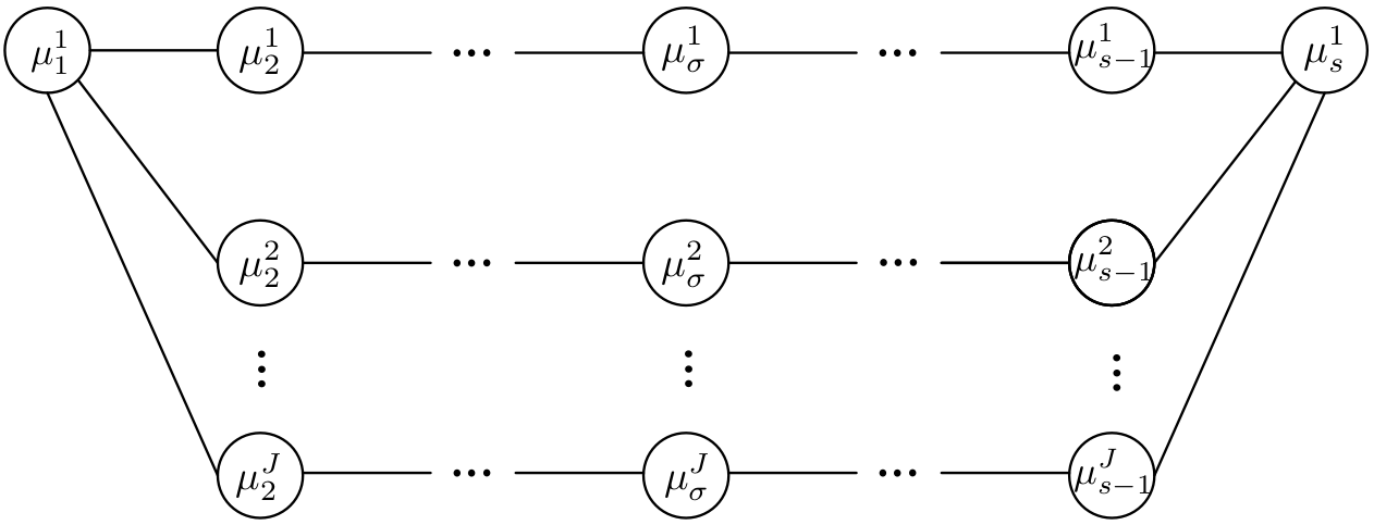
Refer to caption
Figure 4: The graph for series-parallel graph-structured MSBP (Sec. IV-E) with J𝐽J parallel paths of length s𝑠s.

Different from the barycentric MSBP in Sec. IV-D, we now propose another MSBP formulation for the multi-core (J>1𝐽1J>1) case, based on the series-parallel information graph structure in Fig. 4.

This series-parallel graph structured MSBP is motivated by the observation that many software on multi-core computing hardware have notions of input and output terminals. In such applications, the input and output of the computational task are aggregated to a single core. Thus, the information graph structure is induced by measure-valued observations {μσj}(j,σ)subscriptsuperscriptsubscript𝜇𝜎𝑗𝑗𝜎\{\mu_{\sigma}^{j}\}_{(j,\sigma)} where the tuple (j,σ)𝑗𝜎(j,\sigma) belongs to the index set

ΛSP:=(J×s)((J{1})×{1,s}).\displaystyle\Lambda_{\rm{SP}}:=\left(\llbracket J\rrbracket\times\llbracket s\rrbracket\right)\setminus\left(\left(\llbracket J\rrbracket\setminus\{1\}\right)\times\{1,s\}\right). (32)

Although the series-parallel graph in Fig. 4 is not a tree, it has treewidth at most two. So such MSBPs remain computationally tractable as before (see details in Sec. V).

Unlike the formulation in Sec. IV-D, the series-parallel graph structured MSBP formulation does not involve any phantom CPU core. From Fig. 4, the cost (24) now equals

j=1J{cj,1(𝝃i1j,𝝃i2j)+cj,s1(𝝃is1j,𝝃isj)}superscriptsubscript𝑗1𝐽subscript𝑐𝑗1superscriptsubscript𝝃subscript𝑖1𝑗superscriptsubscript𝝃subscript𝑖2𝑗subscript𝑐𝑗𝑠1superscriptsubscript𝝃subscript𝑖𝑠1𝑗superscriptsubscript𝝃subscript𝑖𝑠𝑗\displaystyle\sum_{j=1}^{J}\bigg{\{}c_{j,1}\left(\bm{\xi}_{i_{1}}^{j},\bm{\xi}_{i_{2}}^{j}\right)+c_{j,s-1}\left(\bm{\xi}_{i_{s-1}}^{j},\bm{\xi}_{i_{s}}^{j}\right)\bigg{\}}
+σ=2s1j=1Jcj,σ(𝝃iσj,𝝃iσ+1j).superscriptsubscript𝜎2𝑠1superscriptsubscript𝑗1𝐽subscript𝑐𝑗𝜎superscriptsubscript𝝃subscript𝑖𝜎𝑗superscriptsubscript𝝃subscript𝑖𝜎1𝑗\displaystyle\qquad+\sum_{\sigma=2}^{s-1}\sum_{j=1}^{J}c_{j,\sigma}\left(\bm{\xi}_{i_{\sigma}}^{j},\bm{\xi}_{i_{\sigma+1}}^{j}\right).

By Lemma 1, we find |ΛSP|=J(s2)+2subscriptΛSP𝐽𝑠22|\Lambda_{\rm{SP}}|=J(s-2)+2, and hence for the series-parallel graph structured MSBP, the tensors 𝑪,𝑴(n)0J(s2)+2𝑪𝑴subscriptsuperscriptsuperscript𝑛tensor-productabsent𝐽𝑠22absent0\bm{C},\bm{M}\in\left(\mathbb{R}^{n}\right)^{\otimes J(s-2)+2}_{\geq 0}. In summary, the proposed series-parallel graph-structured MSBP is

min𝑴(n)0(J(s2)+2)𝑪+εlog𝑴,𝑴𝑴subscriptsuperscriptsuperscript𝑛tensor-productabsent𝐽𝑠22absent0𝑪𝜀𝑴𝑴\displaystyle\underset{\bm{M}\in\left(\mathbb{R}^{n}\right)^{\otimes(J(s-2)+2)}_{\geq 0}}{\min}~{}\langle\bm{C}+\varepsilon\log\bm{M},\bm{M}\rangle (33a)
subject toproj(j,σ)(𝑴)=𝝁σj(j,σ)ΛSP.formulae-sequencesubject tosubscriptproj𝑗𝜎𝑴superscriptsubscript𝝁𝜎𝑗for-all𝑗𝜎subscriptΛSP\displaystyle\text{subject to}~{}~{}{\rm{proj}}_{(j,\sigma)}\left(\bm{M}\right)=\bm{\mu}_{\sigma}^{j}\quad\forall(j,\sigma)\in\Lambda_{\rm{SP}}. (33b)

In Sec. V-C, we will discuss the computation of projections (18b) and (22) for the minimizer of (33).

Graph structure MSBP Index set ΛΛ\Lambda
Path tree (Sec. IV-C) (29) sdelimited-⟦⟧𝑠\llbracket s\rrbracket
Barycentric (Sec. IV-D) (31) ΛBCsubscriptΛBC\Lambda_{\rm{BC}} in (30)
Series-parallel (Sec. IV-E) (33) ΛSPsubscriptΛSP\Lambda_{\rm{SP}} in (32)
TABLE I: The index set ΛΛ\Lambda in graph structured MSBPs.

V Algorithms

This section provides algorithmic details and computational complexities to solve the discrete MSBPs (29), (31) and (33).

These MSBPs are strictly convex tensor optimization problems in ns,n(J+1)s,superscript𝑛𝑠superscript𝑛𝐽1𝑠n^{s},n^{(J+1)s}, and nJ(s2)+2superscript𝑛𝐽𝑠22n^{J(s-2)+2} decision variables, respectively, and computationally intractable in general. By leveraging an interplay between duality and graph structures, we will see that it is possible to reduce the computational complexity from exponential to linear in s𝑠s.

Recognizing that (29), (31), (33) are instances of the generic structured optimization problem:

min𝑴(n)0|Λ|𝑪+εlog𝑴,𝑴𝑴subscriptsuperscriptsuperscript𝑛tensor-productabsentΛabsent0𝑪𝜀𝑴𝑴\displaystyle\underset{\bm{M}\in\left(\mathbb{R}^{n}\right)^{\otimes|\Lambda|}_{\geq 0}}{\min}~{}\langle\bm{C}+\varepsilon\log\bm{M},\bm{M}\rangle (34a)
subject toproj(j,σ)(𝑴)=𝝁σj(j,σ)Λ,formulae-sequencesubject tosubscriptproj𝑗𝜎𝑴superscriptsubscript𝝁𝜎𝑗for-all𝑗𝜎Λ\displaystyle\text{subject to}~{}~{}{\rm{proj}}_{(j,\sigma)}\left(\bm{M}\right)=\bm{\mu}_{\sigma}^{j}\quad\forall(j,\sigma)\in\Lambda, (34b)

for suitable index set ΛΛ\Lambda (see Table I), the following is consequence of strong Lagrange duality.

Proposition 3.

[45, 46, 47] Given problem (34), let 𝛌σjnsubscriptsuperscript𝛌𝑗𝜎superscript𝑛\bm{\lambda}^{j}_{\sigma}\in\mathbb{R}^{n} be the Lagrange multipliers for the equality constraints (34b) for all (j,σ)Λ𝑗𝜎Λ(j,\sigma)\in\Lambda. Let

𝑲𝑲\displaystyle\bm{K} :=exp(𝑪/ε)(n)>0|Λ|,assignabsent𝑪𝜀subscriptsuperscriptsuperscript𝑛tensor-productabsentΛabsent0\displaystyle:=\exp(-\bm{C}/\varepsilon)\in\left(\mathbb{R}^{n}\right)^{\otimes|\Lambda|}_{>0}, (35a)
𝒖σjsubscriptsuperscript𝒖𝑗𝜎\displaystyle\bm{u}^{j}_{\sigma} :=exp(𝝀σj/ε)>0n(j,σ)Λ,formulae-sequenceassignabsentsubscriptsuperscript𝝀𝑗𝜎𝜀subscriptsuperscript𝑛absent0for-all𝑗𝜎Λ\displaystyle:=\exp(\bm{\lambda}^{j}_{\sigma}/\varepsilon)\in\mathbb{R}^{n}_{>0}\quad\forall(j,\sigma)\in\Lambda, (35b)
𝑼𝑼\displaystyle\bm{U} :=(j,σ)Λ𝒖σj(n)>0|Λ|.\displaystyle:=\displaystyle\otimes_{(j,\sigma)\in\Lambda}\bm{u}^{j}_{\sigma}\in\left(\mathbb{R}^{n}\right)^{\otimes|\Lambda|}_{>0}. (35c)

Then, the multi-marginal Sinkhorn recursions

𝒖σj𝒖σj𝝁σjproj(j,σ)(𝑲𝑼)(j,σ)Λ,subscriptsuperscript𝒖𝑗𝜎direct-productsubscriptsuperscript𝒖𝑗𝜎subscriptsuperscript𝝁𝑗𝜎subscriptproj𝑗𝜎direct-product𝑲𝑼for-all𝑗𝜎Λ\displaystyle\bm{u}^{j}_{\sigma}\leftarrow\bm{u}^{j}_{\sigma}\odot\bm{\mu}^{j}_{\sigma}\oslash{\rm{proj}}_{(j,\sigma)}\left(\bm{K}\odot\bm{U}\right)~{}\forall(j,\sigma)\in\Lambda, (36)

have guaranteed linear rate of convergence, and the minimizer 𝐌optsuperscript𝐌opt\bm{M}^{\rm{opt}} for (34) is given in terms of the converged 𝐔𝐔\bm{U} as

𝑴opt=𝑲𝑼.superscript𝑴optdirect-product𝑲𝑼\displaystyle\bm{M}^{\rm{opt}}=\bm{K}\odot\bm{U}. (37)

Once 𝑴optsuperscript𝑴opt\bm{M}^{\rm{opt}} is computed, its bimarginal projections of the form (28) yield the probability mass transport matrices between any two marginals. With this, we are able to interpolate between any two marginals to obtain a predicted distribution.

Remark 3.

In our problem, the useful application of this interpolation is as follows: given a time τ[0,t)𝜏0𝑡\tau\in[0,t) and CPU index jJj\in\llbracket J\rrbracket, find σs\sigma\in\llbracket s\rrbracket such that τστ<τσ+1subscript𝜏𝜎𝜏subscript𝜏𝜎1\tau_{\sigma}\leq\tau<\tau_{\sigma+1}, and use the expressions for the bimarginal projections above to compute the bimarginal bridge

Mj,σ:=proj(j,σ),(j,σ+1)(𝑴opt):μσjμσ+1j(0n×n).:assignsuperscript𝑀𝑗𝜎subscriptproj𝑗𝜎𝑗𝜎1superscript𝑴optsuperscriptsubscript𝜇𝜎𝑗annotatedsuperscriptsubscript𝜇𝜎1𝑗absentsubscriptsuperscript𝑛𝑛absent0M^{j,\sigma}:={\rm{proj}}_{(j,\sigma),(j,\sigma+1)}(\bm{M}^{\rm{opt}}):\mu_{\sigma}^{j}\to\mu_{\sigma+1}^{j}\quad\left(\in\mathbb{R}^{n\times n}_{\geq 0}\right).

Using this projection, we can interpolate between μσjsuperscriptsubscript𝜇𝜎𝑗\mu_{\sigma}^{j} and μσ+1jsuperscriptsubscript𝜇𝜎1𝑗\mu_{\sigma+1}^{j} to obtain our estimate μ^τjsuperscriptsubscript^𝜇𝜏𝑗\widehat{\mu}_{\tau}^{j} for the computational resource usage distribution for CPU j𝑗j at time τ𝜏\tau, as

μ^τj:=r=1n=1n[Mr,j,σ]δ(𝝃j𝝃^j(τ,𝝃r,j(τσ),𝝃,j(τσ+1)))assignsuperscriptsubscript^𝜇𝜏𝑗superscriptsubscript𝑟1𝑛superscriptsubscript1𝑛delimited-[]subscriptsuperscript𝑀𝑗𝜎𝑟𝛿superscript𝝃𝑗superscript^𝝃𝑗𝜏superscript𝝃𝑟𝑗subscript𝜏𝜎superscript𝝃𝑗subscript𝜏𝜎1\displaystyle\!\hat{\mu}_{\tau}^{j}\!:=\!\sum_{r=1}^{n}\!\sum_{\ell=1}^{n}\!\left[\!M^{j,\sigma}_{r,\ell}\!\right]\!\!\delta(\bm{\xi}^{j}-\widehat{\bm{\xi}}^{j}(\tau,\bm{\xi}^{r,j}(\tau_{\sigma}),\bm{\xi}^{\ell,j}(\tau_{\sigma+1}))) (38)

where 𝛏^j(τ,𝛏r,j(τσ),𝛏,j(τσ+1)):=(1λ)𝛏r,j(τσ)+λ𝛏,j(τσ+1)assignsuperscript^𝛏𝑗𝜏superscript𝛏𝑟𝑗subscript𝜏𝜎superscript𝛏𝑗subscript𝜏𝜎11𝜆superscript𝛏𝑟𝑗subscript𝜏𝜎𝜆superscript𝛏𝑗subscript𝜏𝜎1\widehat{\bm{\xi}}^{j}(\tau,\bm{\xi}^{r,j}(\tau_{\sigma}),\bm{\xi}^{\ell,j}(\tau_{\sigma+1}))\!\!:=\!(1-\lambda)\bm{\xi}^{r,j}(\tau_{\sigma})\!+\!\lambda\bm{\xi}^{\ell,j}(\tau_{\sigma+1}), and λ:=ττστσ+1τσ[0,1]assign𝜆𝜏subscript𝜏𝜎subscript𝜏𝜎1subscript𝜏𝜎01\lambda:=\dfrac{\tau-\tau_{\sigma}}{\tau_{\sigma+1}-\tau_{\sigma}}\in[0,1].

For numerically solving bi-marginal SBPs (i.e., the case s=2,J=1formulae-sequence𝑠2𝐽1s=2,J=1), the Sinknorn recursions (36) have become the standard [48, 49, 50, 51]. However, applying the same is challenging for MSBPs because computing proj(j,σ)(𝑲𝑼)subscriptproj𝑗𝜎direct-product𝑲𝑼\operatorname*{proj}_{(j,\sigma)}\left(\bm{K}\odot\bm{U}\right) requires 𝒪(n|Λ|)𝒪superscript𝑛Λ\mathcal{O}\left(n^{|\Lambda|}\right) operations. The same issue arises for computing proj(j1,σ1),(j2,σ2)(𝑲𝑼)subscriptprojsubscript𝑗1subscript𝜎1subscript𝑗2subscript𝜎2direct-product𝑲𝑼\operatorname*{proj}_{(j_{1},\sigma_{1}),(j_{2},\sigma_{2})}\left(\bm{K}\odot\bm{U}\right). For both projections, this complexity can be reduced by exploiting the structure of the Hilbert-Schmidt inner product 𝑲,𝑼𝑲𝑼\langle\bm{K},\bm{U}\rangle. Specifically, we make use of the following results from [12].

Lemma 2.

Let the tensor 𝐔𝐔\bm{U} be as in (35c), and consider a tensor 𝐊(n)|Λ|𝐊superscriptsuperscript𝑛tensor-productabsentΛ\bm{K}\in\left(\mathbb{R}^{n}\right)^{\otimes|\Lambda|}.
(i) [12, Lemma 1] For a fixed (j,σ)Λ𝑗𝜎Λ(j,\sigma)\in\Lambda, if 𝐊,𝐔=𝐰1diag(𝐮σj)𝐰2𝐊𝐔superscriptsubscript𝐰1topdiagsubscriptsuperscript𝐮𝑗𝜎subscript𝐰2\langle\bm{K},\bm{U}\rangle=\bm{w}_{1}^{\top}\mathrm{diag}\left(\bm{u}^{j}_{\sigma}\right)\bm{w}_{2} for some vectors 𝐰1,𝐰2nsubscript𝐰1subscript𝐰2superscript𝑛\bm{w}_{1},\bm{w}_{2}\in\mathbb{R}^{n} that do not depend on 𝐮σjsubscriptsuperscript𝐮𝑗𝜎\bm{u}^{j}_{\sigma}, then

proj(j,σ)(𝑲𝑼)=𝒘1𝒖σj𝒘2.subscriptproj𝑗𝜎direct-product𝑲𝑼direct-productsubscript𝒘1subscriptsuperscript𝒖𝑗𝜎subscript𝒘2{\rm{proj}}_{(j,\sigma)}(\bm{K}\odot\bm{U})=\bm{w}_{1}\odot\bm{u}^{j}_{\sigma}\odot\bm{w}_{2}.

(ii) [12, Lemma 2] For fixed (j1,σ1),(j2,σ2)Λsubscript𝑗1subscript𝜎1subscript𝑗2subscript𝜎2Λ(j_{1},\sigma_{1}),(j_{2},\sigma_{2})\in\Lambda, if 𝐊,𝐔=𝐰1diag(𝐮σ1j1)Φdiag(𝐮σ2j2)𝐰3𝐊𝐔superscriptsubscript𝐰1topdiagsubscriptsuperscript𝐮subscript𝑗1subscript𝜎1Φdiagsubscriptsuperscript𝐮subscript𝑗2subscript𝜎2subscript𝐰3\langle\bm{K},\bm{U}\rangle=\bm{w}_{1}^{\top}\mathrm{diag}(\bm{u}^{j_{1}}_{\sigma_{1}})\Phi\mathrm{diag}(\bm{u}^{j_{2}}_{\sigma_{2}})\bm{w}_{3} for some vectors 𝐰1,𝐰3nsubscript𝐰1subscript𝐰3superscript𝑛\bm{w}_{1},\bm{w}_{3}\in\mathbb{R}^{n} and matrix Φn×nΦsuperscript𝑛𝑛\Phi\in\mathbb{R}^{n\times n} where 𝐰1,Φ,𝐰3subscript𝐰1Φsubscript𝐰3\bm{w}_{1},\Phi,\bm{w}_{3} do not depend on 𝐮σ1j1,𝐮σ2j2subscriptsuperscript𝐮subscript𝑗1subscript𝜎1subscriptsuperscript𝐮subscript𝑗2subscript𝜎2\bm{u}^{j_{1}}_{\sigma_{1}},\bm{u}^{j_{2}}_{\sigma_{2}}, then

proj(j1,σ1),(j2,σ2)(𝑲𝑼)=diag(𝒘1𝒖σ1j1)Φdiag(𝒖σ2j2𝒘3).subscriptprojsubscript𝑗1subscript𝜎1subscript𝑗2subscript𝜎2direct-product𝑲𝑼diagdirect-productsubscript𝒘1subscriptsuperscript𝒖subscript𝑗1subscript𝜎1Φdiagdirect-productsubscriptsuperscript𝒖subscript𝑗2subscript𝜎2subscript𝒘3{\rm{proj}}_{(j_{1},\sigma_{1}),(j_{2},\sigma_{2})}(\bm{K}\odot\bm{U})=\mathrm{diag}(\bm{w}_{1}\odot\bm{u}^{j_{1}}_{\sigma_{1}})\Phi\mathrm{diag}(\bm{u}^{j_{2}}_{\sigma_{2}}\odot\bm{w}_{3}).

The special inner product structures in Lemma 2 arises from structured tensors 𝑲𝑲\bm{K} which are in turn induced by the graph structures discussed earlier. Thus, expressing 𝑲,𝑼𝑲𝑼\langle\bm{K},\bm{U}\rangle in the appropriate forms helps compute the desired projections. Below, we show how the imposition of structure on 𝑲𝑲\bm{K} allows this to be done efficiently.

V-A Projections for Path Structured MSBP

For software running on a single CPU core, we have J=1𝐽1J=1 as in Sec. IV-C. The corresponding MSBP is (29). Here, the cost tensor 𝑪𝑪\bm{C} in (24) has a path structure

[𝑪(iσσs)]=[𝑪i1,,is]=σ=1s1[Ciσ,iσ+1σ]\left[\bm{C}_{(i_{\sigma}\mid\sigma\in\llbracket s\rrbracket)}\right]=\left[\bm{C}_{i_{1},\dots,i_{s}}\right]=\sum_{\sigma=1}^{s-1}\left[C_{i_{\sigma},i_{\sigma+1}}^{\sigma}\right] (39)

where the matrix Cσ0n×nsuperscript𝐶𝜎subscriptsuperscript𝑛𝑛absent0C^{\sigma}\in\mathbb{R}^{n\times n}_{\geq 0} encodes the cost of transporting unit mass from {𝝃i(τσ)}i=1nsuperscriptsubscriptsuperscript𝝃𝑖subscript𝜏𝜎𝑖1𝑛\{\bm{\xi}^{i}(\tau_{\sigma})\}_{i=1}^{n} to {𝝃i(τσ+1)}i=1nsuperscriptsubscriptsuperscript𝝃𝑖subscript𝜏𝜎1𝑖1𝑛\{\bm{\xi}^{i}(\tau_{\sigma+1})\}_{i=1}^{n}. This allows us to write 𝑲𝑲\bm{K} in (35a) as

[𝑲(iσσs)]=σ=1s1[Kiσ,iσ+1σ]\left[\bm{K}_{(i_{\sigma}\mid\sigma\in\llbracket s\rrbracket)}\right]=\prod_{\sigma=1}^{s-1}\left[K_{i_{\sigma},i_{\sigma+1}}^{\sigma}\right] (40)

which leads to the following expressions for the marginal projections.

Proposition 4.

[12, Prop. 2], [28, Prop. 1] If 𝐂𝐂\bm{C} has the form (39), Kσ:=exp(Cσ/ε)0n×nassignsuperscript𝐾𝜎superscript𝐶𝜎𝜀subscriptsuperscript𝑛𝑛absent0K^{\sigma}:=\exp(-C^{\sigma}/\varepsilon)\in\mathbb{R}^{n\times n}_{\geq 0}, 𝐊𝐊\bm{K} as in (40), and 𝐔𝐔\bm{U} as in (35c), then (27) and (28) can be expressed as

projσ(𝑲𝑼)=(𝒖1K1k=2σ1diag(𝒖k)Kk)𝒖σ\displaystyle{\rm{proj}}_{\sigma}\!\left(\bm{K}\odot\bm{U}\right)\!=\!\!\left(\!\bm{u}_{1}^{\!\top}K^{1}\!\prod_{k=2}^{\sigma-1}\!\mathrm{diag}(\bm{u}_{k})K^{k}\!\!\right)^{\!\!\top}\!\!\!\!\odot\bm{u}_{\sigma}\odot
((k=σ+1s1Kk1diag(𝒖k))Ks1𝒖s)σs,\displaystyle\left(\!\!\left(\prod_{k=\sigma+1}^{s-1}K^{k-1}\mathrm{diag}(\bm{u}_{k})\!\right)\!\!K^{s-1}\bm{u}_{s}\!\right)\,\forall\sigma\in\llbracket s\rrbracket, (41)

and projσ1,σ2(𝐊𝐔)=subscriptprojsubscript𝜎1subscript𝜎2direct-product𝐊𝐔absent{\rm{proj}}_{\sigma_{1},\sigma_{2}}\!\left(\bm{K}\odot\bm{U}\right)=

diag(𝒖1K1k=2σ11diag(𝒖k)Kk)k=σ1+1σ2(Kk1diag(𝒖k))diagsuperscriptsubscript𝒖1topsuperscript𝐾1superscriptsubscriptproduct𝑘2subscript𝜎11diagsubscript𝒖𝑘superscript𝐾𝑘superscriptsubscriptproduct𝑘subscript𝜎11subscript𝜎2superscript𝐾𝑘1diagsubscript𝒖𝑘\displaystyle\mathrm{diag}\!\left(\!\!\bm{u}_{1}^{\top}K^{1}\prod_{k=2}^{\sigma_{1}-1}\mathrm{diag}(\bm{u}_{k})K^{k}\!\!\right)\prod_{k=\sigma_{1}+1}^{\sigma_{2}}\!\!\left(K^{k-1}\mathrm{diag}(\bm{u}_{k})\right)
diag((k=σ2+1s1Kk1diag(𝒖k))Ks1𝒖s)diagsuperscriptsubscriptproduct𝑘subscript𝜎21𝑠1superscript𝐾𝑘1diagsubscript𝒖𝑘superscript𝐾𝑠1subscript𝒖𝑠\displaystyle\mathrm{diag}\!\left(\!\!\left(\prod_{k=\sigma_{2}+1}^{s-1}K^{k-1}\mathrm{diag}(\bm{u}_{k})\!\!\right)\!K^{s-1}\bm{u}_{s}\!\!\right)
(σ1,σ2){s2σ1<σ2}.\displaystyle\qquad\qquad\qquad\qquad~{}\forall(\sigma_{1},\sigma_{2})\in\{\llbracket s\rrbracket^{\otimes 2}\mid\sigma_{1}<\sigma_{2}\}. (42)

Observe that even the naïve computation of (41) is dominated by 2s42𝑠42s-4 matrix-vector multiplications (by cancellation, (36) can be computed by s1𝑠1s-1 such multiplications; see [28, Remark 3]). Since such multiplications have 𝒪(n2)𝒪superscript𝑛2\mathcal{O}(n^{2}) complexity, each Sinkhorn iteration has 𝒪((s1)n2)𝒪𝑠1superscript𝑛2\mathcal{O}\left((s-1)n^{2}\right) complexity – linear in s𝑠s, and a great improvement from the general 𝒪(ns)𝒪superscript𝑛𝑠\mathcal{O}(n^{s}) complexity of the method. Our method’s 𝒪((s1)n2)𝒪𝑠1superscript𝑛2\mathcal{O}\left((s-1)n^{2}\right) complexity is sharp for exact computation. The recent work [52] reduces the complexity in n𝑛n from quadratic to linear at the expense of approximate computation.

Remark 4.

While it is clear from their expressions that the bimarginal projection (42) has similar order-of-magnitude complexity to the unimarginal projection (41), hereafter we focus only on the complexity of the latter, as these are performed every Sinkhorn iteration until the method converges. Following this, bimarginal projections of the solution 𝐌optsuperscript𝐌opt\bm{M}^{\rm{opt}} onto each pair of marginals of interest are to be performed only once a posteriori, and so exact floating-point operational count for these projections is not critical.

V-B Projections for Barycentric MSBP

For software running on multiple CPU cores, we have J>1𝐽1J>1. The corresponding barycentric MSBP (31) formulated in Sec. IV-D involves a tree that is more general than a path.

In this subsection, we let n0subscript𝑛0n_{0} denote the number of samples in the barycentric CPU. For the sake of generality, here we derive the complexity for the projections in terms of n𝑛n and n0subscript𝑛0n_{0}. Then, 𝑪,𝑴,𝑼(n)0Js(n0)0s𝑪𝑴𝑼tensor-productsubscriptsuperscriptsuperscript𝑛tensor-productabsent𝐽𝑠absent0subscriptsuperscriptsuperscriptsubscript𝑛0tensor-productabsent𝑠absent0\bm{C},\bm{M},\bm{U}\in\left(\mathbb{R}^{n}\right)^{\otimes Js}_{\geq 0}\otimes\left(\mathbb{R}^{n_{0}}\right)^{\otimes s}_{\geq 0}. For n0nsubscript𝑛0𝑛n_{0}\neq n, formulation (34)-(35) applies mutatis-mutandis.

Recall that here the index set Λ=ΛBCΛsubscriptΛBC\Lambda=\Lambda_{\rm{BC}} as in (30). The cost tensor 𝑪𝑪\bm{C} for barycentric MSBP takes the form

[𝑪(i(j,σ)(j,σ)ΛBC)]=σ=1s1[Ci(0,σ),i(0,σ+1)0,σ]delimited-[]subscript𝑪conditionalsubscript𝑖𝑗𝜎𝑗𝜎subscriptΛBCsuperscriptsubscript𝜎1𝑠1delimited-[]superscriptsubscript𝐶subscript𝑖0𝜎subscript𝑖0𝜎10𝜎\displaystyle\left[\bm{C}_{(i_{(j,\sigma)}\mid(j,\sigma)\in\Lambda_{\rm{BC}})}\right]=\sum_{\sigma=1}^{s-1}\left[C_{i_{(0,\sigma)},i_{(0,\sigma+1)}}^{0,\sigma}\right]
+σ=1sj=1J[Ci(j,σ),i(0,σ)j,σ]superscriptsubscript𝜎1𝑠superscriptsubscript𝑗1𝐽delimited-[]superscriptsubscript𝐶subscript𝑖𝑗𝜎subscript𝑖0𝜎𝑗𝜎\displaystyle+\sum_{\sigma=1}^{s}\sum_{j=1}^{J}\left[C_{i_{(j,\sigma)},i_{(0,\sigma)}}^{j,\sigma}\right] (43)

where the matrices C0,σ0n0×n0superscript𝐶0𝜎subscriptsuperscriptsubscript𝑛0subscript𝑛0absent0C^{0,\sigma}\in\mathbb{R}^{n_{0}\times n_{0}}_{\geq 0} are the ground cost matrices between barycenters 𝝃0(τσ)superscript𝝃0subscript𝜏𝜎\bm{\xi}^{0}(\tau_{\sigma}) and 𝝃0(τσ+1)superscript𝝃0subscript𝜏𝜎1\bm{\xi}^{0}(\tau_{\sigma+1}) for σs1\sigma\in\llbracket s-1\rrbracket, whereas Cj,σ0n0×nsuperscript𝐶𝑗𝜎subscriptsuperscriptsubscript𝑛0𝑛absent0C^{j,\sigma}\in\mathbb{R}^{n_{0}\times{n}}_{\geq 0} are those between the CPU marginals 𝝃j(τσ)superscript𝝃𝑗subscript𝜏𝜎\bm{\xi}^{j}(\tau_{\sigma}) and their barycenters 𝝃0(τσ)superscript𝝃0subscript𝜏𝜎\bm{\xi}^{0}(\tau_{\sigma}), for (j,σ)J×s(j,\sigma)\in\llbracket J\rrbracket\times\llbracket s\rrbracket. So now, we can write 𝑲𝑲\bm{K} in (35a) as

[𝑲(i(j,σ)(j,σ)ΛBC)]delimited-[]subscript𝑲conditionalsubscript𝑖𝑗𝜎𝑗𝜎subscriptΛBC\displaystyle\left[\bm{K}_{(i_{(j,\sigma)}\mid(j,\sigma)\in\Lambda_{\rm{BC}})}\right]
=(σ=1s1[Ki(0,σ),i(0,σ+1)0,σ])×σ=1sj=1J[Ki(j,σ),i(0,σ)j,σ].absentsuperscriptsubscriptproduct𝜎1𝑠1delimited-[]superscriptsubscript𝐾subscript𝑖0𝜎subscript𝑖0𝜎10𝜎superscriptsubscriptproduct𝜎1𝑠superscriptsubscriptproduct𝑗1𝐽delimited-[]superscriptsubscript𝐾subscript𝑖𝑗𝜎subscript𝑖0𝜎𝑗𝜎\displaystyle=\bigg{(}\prod_{\sigma=1}^{s-1}\left[K_{i_{(0,\sigma)},i_{(0,\sigma+1)}}^{0,\sigma}\right]\bigg{)}\times\prod_{\sigma=1}^{s}\prod_{j=1}^{J}\left[K_{i_{(j,\sigma)},i_{(0,\sigma)}}^{j,\sigma}\right]. (44)

With this, the projections can be computed as follows (proof in Appendix -A).

Proposition 5.

If 𝐂𝐂\bm{C} has the form (43), Kj,σ:=exp(Cj,σ/ε)assignsuperscript𝐾𝑗𝜎superscript𝐶𝑗𝜎𝜀K^{j,\sigma}:=\exp(-C^{j,\sigma}/\varepsilon), 𝐊𝐊\bm{K} as in (44), and 𝐔𝐔\bm{U} as in (35c), then the projections (27) and (28) can be expressed as

proj(0,σ)(𝑲𝑼)=(𝒑1K0,1k=2σ1diag(𝒑k)K0,k)𝒑σ\displaystyle{\rm{proj}}_{(0,\sigma)}\!\left(\bm{K}\odot\bm{U}\right)\!=\!\!\left(\!\bm{p}_{1}^{\!\top}K^{0,1}\!\prod_{k=2}^{\sigma-1}\!\mathrm{diag}(\bm{p}_{k})K^{0,k}\!\!\right)^{\!\!\top}\!\!\!\!\odot\bm{p}_{\sigma}\odot
((k=σ+1s1K0,k1diag(𝒑k))K0,s1𝒑s)σs,\displaystyle\quad\left(\!\!\left(\prod_{k=\sigma+1}^{s-1}K^{0,k-1}\mathrm{diag}(\bm{p}_{k})\!\right)\!\!K^{0,s-1}\bm{p}_{s}\!\right)\quad\forall\sigma\in\llbracket s\rrbracket, (45a)
proj(j,σ)(𝑲𝑼)=𝒖σjKj,σ((𝒑1K0,1k=2σ1diag(𝒑k)K0,k)\displaystyle{\rm{proj}}_{(j,\sigma)}\!\left(\bm{K}\odot\bm{U}\right)\!=\bm{u}_{\sigma}^{j}\odot{K^{j,\sigma}}^{\top}\!\Bigg{(}\!\!\left(\!\bm{p}_{1}^{\!\top}K^{0,1}\!\prod_{k=2}^{\sigma-1}\!\mathrm{diag}(\bm{p}_{k})K^{0,k}\!\!\right)^{\!\!\top}
(𝒑σ(Kj,σ𝒖σj))((k=σ+1s1K0,k1diag(𝒑k))K0,s1𝒑s)direct-productabsentdirect-productsubscript𝒑𝜎superscript𝐾𝑗𝜎superscriptsubscript𝒖𝜎𝑗superscriptsubscriptproduct𝑘𝜎1𝑠1superscript𝐾0𝑘1diagsubscript𝒑𝑘superscript𝐾0𝑠1subscript𝒑𝑠\displaystyle\odot\left(\bm{p}_{\sigma}\oslash\left({K^{j,\sigma}}\bm{u}_{\sigma}^{j}\right)\right)\odot\left(\!\!\left(\prod_{k=\sigma+1}^{s-1}K^{0,k-1}\mathrm{diag}(\bm{p}_{k})\!\right)\!\!K^{0,s-1}\bm{p}_{s}\!\!\right)
(j,σ)J×s,\displaystyle\qquad\qquad\qquad\qquad\qquad\qquad\forall(j,\sigma)\in\llbracket J\rrbracket\times\llbracket s\rrbracket, (45b)

and for (j,σ)J×s(j,\sigma)\in\llbracket J\rrbracket\times\llbracket s\rrbracket and σ1,σ2s\sigma_{1},\sigma_{2}\in\llbracket s\rrbracket such that σ1<σ2subscript𝜎1subscript𝜎2\sigma_{1}<\sigma_{2},

proj(0,σ),(j,σ)(𝑲𝑼)=diag(𝒖σ0)diag(K0,σ1𝝆(0,σ),(j,σ))subscriptproj0𝜎𝑗𝜎direct-product𝑲𝑼diagsuperscriptsubscript𝒖𝜎0diagsuperscriptsuperscript𝐾0𝜎1topsubscript𝝆0𝜎𝑗𝜎\displaystyle{\rm{proj}}_{(0,\sigma),(j,\sigma)}\!\left(\bm{K}\odot\bm{U}\right)=\mathrm{diag}(\bm{u}_{\sigma}^{0})\mathrm{diag}\left({K^{0,\sigma-1}}^{\top}\bm{\rho}_{(0,\sigma),(j,\sigma)}\right)
Kj,σdiag(𝒖σj),superscript𝐾𝑗𝜎diagsuperscriptsubscript𝒖𝜎𝑗\displaystyle\quad\quad\quad\quad\quad\quad\quad\quad\quad\quad\quad{K^{j,\sigma}}\mathrm{diag}(\bm{u}_{\sigma}^{j}), (46a)
proj(0,σ1),(0,σ2)(𝑲𝑼)=diag(𝒑1K0,1k=2σ11diag(𝒑k)K0,k)subscriptproj0subscript𝜎10subscript𝜎2direct-product𝑲𝑼diagsuperscriptsubscript𝒑1topsuperscript𝐾01superscriptsubscriptproduct𝑘2subscript𝜎11diagsubscript𝒑𝑘superscript𝐾0𝑘\displaystyle{\rm{proj}}_{(0,\sigma_{1}),(0,\sigma_{2})}\!\left(\bm{K}\odot\bm{U}\right)=\mathrm{diag}\!\left(\!\!\bm{p}_{1}^{\top}K^{0,1}\prod_{k=2}^{\sigma_{1}-1}\mathrm{diag}(\bm{p}_{k})K^{0,k}\!\!\right)
diag(𝒑σ1)k=σ1+1σ2(K0,k1diag(𝒑k))direct-productabsentdiagsubscript𝒑subscript𝜎1superscriptsubscriptproduct𝑘subscript𝜎11subscript𝜎2superscript𝐾0𝑘1diagsubscript𝒑𝑘\displaystyle\qquad\qquad\qquad\qquad~{}~{}~{}\odot\mathrm{diag}(\bm{p}_{\sigma_{1}})\!\!\prod_{k=\sigma_{1}+1}^{\sigma_{2}}\!\!\left(K^{0,k-1}\mathrm{diag}(\bm{p}_{k})\right)
diag((k=σ2+1s1K0,k1diag(𝒑k))K0,s1𝒑s)direct-productabsentdiagsuperscriptsubscriptproduct𝑘subscript𝜎21𝑠1superscript𝐾0𝑘1diagsubscript𝒑𝑘superscript𝐾0𝑠1subscript𝒑𝑠\displaystyle\qquad\qquad\qquad~{}\odot\mathrm{diag}\!\left(\!\!\left(\prod_{k=\sigma_{2}+1}^{s-1}K^{0,k-1}\mathrm{diag}(\bm{p}_{k})\!\!\right)\!K^{0,s-1}\bm{p}_{s}\!\!\right) (46b)

where 𝐩σ:=𝐮σ0(jJKj,σ𝐮σj)assignsubscript𝐩𝜎direct-productsuperscriptsubscript𝐮𝜎0subscript𝑗delimited-⟦⟧𝐽superscript𝐾𝑗𝜎superscriptsubscript𝐮𝜎𝑗\bm{p}_{\sigma}:=\bm{u}_{\sigma}^{0}\odot(\bigodot_{j\in\llbracket J\rrbracket}K^{j,\sigma}\bm{u}_{\sigma}^{j}) for σs\sigma\in\llbracket s\rrbracket, and

𝝆(0,σ),(j,σ)subscript𝝆0𝜎𝑗𝜎\displaystyle\bm{\rho}_{(0,\sigma),(j,\sigma)} :=(𝒑1K0,1k=2σ1diag(𝒑k)K0,k)assignabsentsuperscriptsuperscriptsubscript𝒑1topsuperscript𝐾01superscriptsubscriptproduct𝑘2𝜎1diagsubscript𝒑𝑘superscript𝐾0𝑘top\displaystyle:=\!\!\left(\!\bm{p}_{1}^{\!\top}K^{0,1}\!\prod_{k=2}^{\sigma-1}\!\mathrm{diag}(\bm{p}_{k})K^{0,k}\!\!\right)^{\!\!\top}
(𝒑σ(𝒖σ0Kj,σ𝒖σj))\displaystyle\quad\odot\left(\bm{p}_{\sigma}\oslash\left(\bm{u}_{\sigma}^{0}\odot K^{j,\sigma}\bm{u}_{\sigma}^{j}\right)\right)\odot
((k=σ+1s1K0,k1diag(𝒑k))K0,s1𝒑s)σs.\displaystyle\left(\!\!\left(\prod_{k=\sigma+1}^{s-1}K^{0,k-1}\mathrm{diag}(\bm{p}_{k})\!\right)\!\!K^{0,s-1}\bm{p}_{s}\!\right)\quad\forall\sigma\in\llbracket s\rrbracket.

Similar to the single-core case in the Sec. V-A, the computational complexity for all projections in Proposition 5 are linear in J𝐽J and s𝑠s. Specifically, the computation of the s𝑠s 𝒑σsubscript𝒑𝜎\bm{p}_{\sigma} vectors in Proposition 5 requires a total of Js𝐽𝑠Js matrix-vector multiplications, and the total number of floating-point operations when projecting onto a barycenter (as in (45a)) is

Js(n0n+n0)+(2n0)+(2s2)n02.𝐽𝑠subscript𝑛0𝑛subscript𝑛02subscript𝑛02𝑠2superscriptsubscript𝑛02Js(n_{0}n+n_{0})+\left(2n_{0}\right)+(2s-2)n_{0}^{2}. (47)

The number of floating-point operations when projecting onto a non-barycentric marginal (as in (45b)) is

Js(n0n+n0)+(3n0+n+2n0n)+(2s2)n02.𝐽𝑠subscript𝑛0𝑛subscript𝑛03subscript𝑛0𝑛2subscript𝑛0𝑛2𝑠2superscriptsubscript𝑛02Js(n_{0}n+n_{0})+\left(3n_{0}+n+2n_{0}n\right)+(2s-2)n_{0}^{2}. (48)

V-C Projections for Series-Parallel Graph-structured MSBP

The series-parallel graph-structured MSBP (33) formulated in Sec. IV-E involves a series-parallel graph which is not a tree. Recall that the corresponding index set Λ=ΛSPΛsubscriptΛSP\Lambda=\Lambda_{\rm{SP}} as in (32). For any fixed jJj\in\llbracket J\rrbracket, let

ΛSPj:={j}×(s{1,s}).\Lambda_{\rm{SP}}^{j}:=\{j\}\times\left(\llbracket s\rrbracket\setminus\{1,s\}\right).

Then, the cost tensor 𝑪𝑪\bm{C} for series-parallel graph-structured MSBP takes the form

[𝑪(i(j,σ)(j,σ)ΛSP)]=j=1J[𝑪i(1,1),(i(j,σ)(j,σ)ΛSPj),i(1,s)j]delimited-[]subscript𝑪conditionalsubscript𝑖𝑗𝜎𝑗𝜎subscriptΛSPsuperscriptsubscript𝑗1𝐽delimited-[]superscriptsubscript𝑪subscript𝑖11conditionalsubscript𝑖𝑗𝜎𝑗𝜎superscriptsubscriptΛSP𝑗subscript𝑖1𝑠𝑗\displaystyle\left[\!\bm{C}_{(i_{(j,\sigma)}\mid(j,\sigma)\in\Lambda_{\rm{SP}})}\!\right]=\!\sum_{j=1}^{J}\!\left[\!\bm{C}_{i_{(1,1)},(i_{(j,\sigma)}\mid(j,\sigma)\in\Lambda_{\rm{SP}}^{j}),i_{(1,s)}}^{j}\!\right] (49)

where each 𝑪j(n)>0ssuperscript𝑪𝑗subscriptsuperscriptsuperscript𝑛tensor-productabsent𝑠absent0\bm{C}^{j}\in\left(\mathbb{R}^{n}\right)^{\otimes s}_{>0} is the path-structured cost tensor along the j𝑗jth CPU’s path, i.e.,

[𝑪i(1,1),(i(j,σ)(j,σ)ΛSPj),i(1,s)j]=Ci(1,1),i(j,2)j,1delimited-[]superscriptsubscript𝑪subscript𝑖11conditionalsubscript𝑖𝑗𝜎𝑗𝜎superscriptsubscriptΛSP𝑗subscript𝑖1𝑠𝑗subscriptsuperscript𝐶𝑗1subscript𝑖11subscript𝑖𝑗2\displaystyle\left[\bm{C}_{i_{(1,1)},(i_{(j,\sigma)}\mid(j,\sigma)\in\Lambda_{\rm{SP}}^{j}),i_{(1,s)}}^{j}\right]=C^{j,1}_{i_{(1,1)},i_{(j,2)}}
+σ=2s2Ci(j,σ),i(j,σ+1)j,σ+Ci(j,s1),i(1,s)j,s1,superscriptsubscript𝜎2𝑠2subscriptsuperscript𝐶𝑗𝜎subscript𝑖𝑗𝜎subscript𝑖𝑗𝜎1subscriptsuperscript𝐶𝑗𝑠1subscript𝑖𝑗𝑠1subscript𝑖1𝑠\displaystyle+\sum_{\sigma=2}^{s-2}C^{j,\sigma}_{i_{(j,\sigma)},i_{(j,\sigma+1)}}+C^{j,s-1}_{i_{(j,s-1)},i_{(1,s)}}, (50)

wherein the matrices Cj,10n×nsuperscript𝐶𝑗1subscriptsuperscript𝑛𝑛absent0C^{j,1}\in\mathbb{R}^{{n}\times{n}}_{\geq 0} are the ground cost matrices between marginals 𝝃1(τ1)superscript𝝃1subscript𝜏1\bm{\xi}^{1}(\tau_{1}) and 𝝃j(τ2)superscript𝝃𝑗subscript𝜏2\bm{\xi}^{j}(\tau_{2}) for jJj\in\llbracket J\rrbracket, and similarly Cj,s1superscript𝐶𝑗𝑠1C^{j,s-1} maps between 𝝃j(τs1)superscript𝝃𝑗subscript𝜏𝑠1\bm{\xi}^{j}(\tau_{s-1}) and 𝝃1(τs)superscript𝝃1subscript𝜏𝑠\bm{\xi}^{1}(\tau_{s}). When σs2{1}\sigma\in\llbracket s-2\rrbracket\setminus\{1\}, the matrices Cj,σsuperscript𝐶𝑗𝜎C^{j,\sigma} map between 𝝃j(τσ)superscript𝝃𝑗subscript𝜏𝜎\bm{\xi}^{j}(\tau_{\sigma}) and 𝝃j(τσ+1)superscript𝝃𝑗subscript𝜏𝜎1\bm{\xi}^{j}(\tau_{\sigma+1}).

Consequently, we write 𝑲𝑲\bm{K} in (35a) as

[𝑲(i(j,σ)(j,σ)ΛSP)]=j=1J[𝑲i(1,1),(i(j,σ)(j,σ)ΛSPj),i(1,s)j],delimited-[]subscript𝑲conditionalsubscript𝑖𝑗𝜎𝑗𝜎subscriptΛSPsuperscriptsubscriptproduct𝑗1𝐽delimited-[]superscriptsubscript𝑲subscript𝑖11conditionalsubscript𝑖𝑗𝜎𝑗𝜎superscriptsubscriptΛSP𝑗subscript𝑖1𝑠𝑗\displaystyle\!\!\left[\!\bm{K}_{(i_{(j,\sigma)}\mid(j,\sigma)\in\Lambda_{\rm{SP}})}\!\right]\!\!=\!\!\prod_{j=1}^{J}\!\left[\!\bm{K}_{i_{(1,1)},(i_{(j,\sigma)}\mid(j,\sigma)\in\Lambda_{\rm{SP}}^{j}),i_{(1,s)}}^{j}\!\right], (51a)
[𝑲i(1,1),(i(j,σ)(j,σ)ΛSPj),i(1,s)j]=Ki(1,1),i(j,2)j,1,delimited-[]superscriptsubscript𝑲subscript𝑖11conditionalsubscript𝑖𝑗𝜎𝑗𝜎superscriptsubscriptΛSP𝑗subscript𝑖1𝑠𝑗subscriptsuperscript𝐾𝑗1subscript𝑖11subscript𝑖𝑗2\displaystyle\left[\bm{K}_{i_{(1,1)},(i_{(j,\sigma)}\mid(j,\sigma)\in\Lambda_{\rm{SP}}^{j}),i_{(1,s)}}^{j}\right]=K^{j,1}_{i_{(1,1)},i_{(j,2)}},
(σ=2s2Ki(j,σ),i(j,σ+1)j,σ)Ki(j,s1),i(1,s)j,s1,absentsuperscriptsubscriptproduct𝜎2𝑠2subscriptsuperscript𝐾𝑗𝜎subscript𝑖𝑗𝜎subscript𝑖𝑗𝜎1subscriptsuperscript𝐾𝑗𝑠1subscript𝑖𝑗𝑠1subscript𝑖1𝑠\displaystyle\quad\quad\quad\quad\quad\quad\cdot\left(\prod_{\sigma=2}^{s-2}K^{j,\sigma}_{i_{(j,\sigma)},i_{(j,\sigma+1)}}\right)K^{j,s-1}_{i_{(j,s-1)},i_{(1,s)}}, (51b)

and the associated projections can be expressed as follows (proof in Appendix -B).

Proposition 6.

If 𝐂𝐂\bm{C} has the form (49), Kj,σ:=exp(Cj,σ/ε)assignsuperscript𝐾𝑗𝜎superscript𝐶𝑗𝜎𝜀K^{j,\sigma}:=\exp(-C^{j,\sigma}/\varepsilon), 𝐊𝐊\bm{K} as in (51), and 𝐔𝐔\bm{U} as in (35c), then letting

Ak:=Kk,1(σ=2s1diag(𝒖σk)Kk,σ),assignsubscript𝐴𝑘superscript𝐾𝑘1superscriptsubscriptproduct𝜎2𝑠1diagsuperscriptsubscript𝒖𝜎𝑘superscript𝐾𝑘𝜎\displaystyle A_{k}:=K^{k,1}\left(\prod_{\sigma=2}^{s-1}\mathrm{diag}(\bm{u}_{\sigma}^{k})K^{k,\sigma}\right), (52)

the projection (27) takes the form

proj(1,1)(𝑲𝑼)subscriptproj11direct-product𝑲𝑼\displaystyle{\rm{proj}}_{(1,1)}\!\left(\bm{K}\odot\bm{U}\right)\! =𝒖11(k=1JAk)𝒖s1,absentdirect-productsuperscriptsubscript𝒖11superscriptsubscriptproduct𝑘1𝐽subscript𝐴𝑘superscriptsubscript𝒖𝑠1\displaystyle=\bm{u}_{1}^{1}\odot\left(\prod_{k=1}^{J}A_{k}\right)\bm{u}_{s}^{1}, (53a)
proj(1,s)(𝑲𝑼)subscriptproj1𝑠direct-product𝑲𝑼\displaystyle{\rm{proj}}_{(1,s)}\!\left(\bm{K}\odot\bm{U}\right)\! =(𝒖11k=1JAk)𝒖s1,absentdirect-productsuperscriptsuperscriptsuperscriptsubscript𝒖11topsuperscriptsubscriptproduct𝑘1𝐽subscript𝐴𝑘topsuperscriptsubscript𝒖𝑠1\displaystyle=\left({\bm{u}_{1}^{1}}^{\top}\prod_{k=1}^{J}A_{k}\right)^{\top}\odot\bm{u}_{s}^{1}, (53b)
proj(j,σ)(𝑲𝑼)subscriptproj𝑗𝜎direct-product𝑲𝑼\displaystyle{\rm{proj}}_{(j,\sigma)}\!\left(\bm{K}\odot\bm{U}\right)\! =(𝒖11(k=1j1Ak)Kj,1\displaystyle=\Bigg{(}{\bm{u}_{1}^{1}}^{\top}\bigg{(}\prod_{k=1}^{j-1}A_{k}\bigg{)}K^{j,1}
(m=2σ1diag(𝒖mj)Kj,m))𝒖σj\displaystyle\bigg{(}\prod_{m=2}^{\sigma-1}\mathrm{diag}(\bm{u}_{m}^{j})K^{j,m}\bigg{)}\Bigg{)}^{\top}\odot\bm{u}_{\sigma}^{j}\odot
(Kj,σ(m=σ+1s1\displaystyle\Bigg{(}K^{j,\sigma}\bigg{(}\prod_{m=\sigma+1}^{s-1} diag(𝒖mj)Kj,m)(k=j+1JAk)𝒖s1),\displaystyle\mathrm{diag}(\bm{u}_{m}^{j})K^{j,m}\bigg{)}\bigg{(}\prod_{k=j+1}^{J}A_{k}\bigg{)}\bm{u}_{s}^{1}\Bigg{)}, (53c)

where (j,σ)kJΛSPk𝑗𝜎subscript𝑘delimited-⟦⟧𝐽superscriptsubscriptΛSP𝑘(j,\sigma)\in\bigcup_{k\in\llbracket J\rrbracket}\Lambda_{\rm{SP}}^{k} in (53c). Furthermore, the projection (28) can be expressed as

proj(1,1),(j,2)(𝑲𝑼)=diag(𝒖11)(k=1j1Ak)Kj,1subscriptproj11𝑗2direct-product𝑲𝑼diagsuperscriptsubscript𝒖11superscriptsubscriptproduct𝑘1𝑗1subscript𝐴𝑘superscript𝐾𝑗1\displaystyle{\rm{proj}}_{(1,1),(j,2)}\!\left(\bm{K}\odot\bm{U}\right)\!=\mathrm{diag}\left(\bm{u}_{1}^{1}\right)\cdot\bigg{(}\prod_{k=1}^{j-1}A_{k}\bigg{)}K^{j,1}
diag(𝒖2jKj,2(k=3s1diag(𝒖kj)Kj,k)(k=j+1JAk)𝒖s1),absentdiagdirect-productsuperscriptsubscript𝒖2𝑗superscript𝐾𝑗2superscriptsubscriptproduct𝑘3𝑠1diagsuperscriptsubscript𝒖𝑘𝑗superscript𝐾𝑗𝑘superscriptsubscriptproduct𝑘𝑗1𝐽subscript𝐴𝑘superscriptsubscript𝒖𝑠1\displaystyle\cdot\mathrm{diag}\left(\bm{u}_{2}^{j}\odot K^{j,2}\bigg{(}\prod_{k=3}^{s-1}\mathrm{diag}(\bm{u}_{k}^{j})K^{j,k}\bigg{)}\bigg{(}\prod_{k=j+1}^{J}A_{k}\bigg{)}\bm{u}_{s}^{1}\right), (54a)
proj(j,s1),(1,s)(𝑲𝑼)=diag((𝒖11(k=1j1Ak)Kj,1\displaystyle{\rm{proj}}_{(j,s-1),(1,s)}\!\left(\bm{K}\odot\bm{U}\right)\!=\mathrm{diag}\Bigg{(}\Bigg{(}{\bm{u}_{1}^{1}}^{\top}\bigg{(}\prod_{k=1}^{j-1}A_{k}\bigg{)}K^{j,1}
(k=2s2diag(𝒖kj)Kj,k))𝒖s1j)Kj,s1(k=j+1JAk)\displaystyle\bigg{(}\prod_{k=2}^{s-2}\mathrm{diag}(\bm{u}_{k}^{j})K^{j,k}\bigg{)}\Bigg{)}^{\top}\odot\bm{u}_{s-1}^{j}\Bigg{)}\cdot K^{j,s-1}\bigg{(}\prod_{k=j+1}^{J}A_{k}\bigg{)}
diag(𝒖s1),absentdiagsuperscriptsubscript𝒖𝑠1\displaystyle\cdot\mathrm{diag}\left(\bm{u}_{s}^{1}\right), (54b)
proj(j,σ),(j,σ+1)(𝑲𝑼)=diag((𝒖11(k=1j1Ak)Kj,1\displaystyle{\rm{proj}}_{(j,\sigma),(j,\sigma+1)}\!\left(\bm{K}\odot\bm{U}\right)\!=\mathrm{diag}\Bigg{(}\Bigg{(}{\bm{u}_{1}^{1}}^{\top}\bigg{(}\prod_{k=1}^{j-1}A_{k}\bigg{)}K^{j,1}
(k=2σ1diag(𝒖kj)Kj,k))𝒖σj)Kj,σdiag(𝒖σ+1j\displaystyle\bigg{(}\prod_{k=2}^{\sigma-1}\mathrm{diag}(\bm{u}_{k}^{j})K^{j,k}\bigg{)}\Bigg{)}^{\top}\odot\bm{u}_{\sigma}^{j}\Bigg{)}\cdot K^{j,\sigma}\cdot\mathrm{diag}\Bigg{(}\bm{u}_{\sigma+1}^{j}
Kj,σ+1(j=σ+2s1diag(𝒖kj)Kj,k)(k=j+1JAk)𝒖s1).\displaystyle\odot K^{j,\sigma+1}\Bigg{(}\prod_{j=\sigma+2}^{s-1}\mathrm{diag}(\bm{u}_{k}^{j})K^{j,k}\bigg{)}\bigg{(}\prod_{k=j+1}^{J}A_{k}\bigg{)}\bm{u}_{s}^{1}\Bigg{)}. (54c)

Directly computing (52) requires 1+2(s2)12𝑠21+2(s-2) matrix-matrix multiplications, each in this case involving n3superscript𝑛3n^{3} floating-point operations. However, since all unimarginal projections result in a vector, (53) involves only matrix-vector multiplications (n2superscript𝑛2n^{2} operations) and elementwise vector multiplication (n𝑛n operations). We can see that (53a) and (53b) each involve

n+J(1+2(s2))n2𝑛𝐽12𝑠2superscript𝑛2n+J\left(1+2(s-2)\right)n^{2} (55)

operations, and (53c) involves

2n+J(1+2(s2))n2n22𝑛𝐽12𝑠2superscript𝑛2superscript𝑛22n+J\left(1+2(s-2)\right)n^{2}-n^{2} (56)

such operations.

Remark 5.

For n0=n,s2,J2formulae-sequencesubscript𝑛0𝑛formulae-sequence𝑠2𝐽2n_{0}=n,s\geq 2,J\geq 2, we note that

the expression(48)=(Js+2s)n2+(Js+4)n8n2+8n.the expressionitalic-(48italic-)𝐽𝑠2𝑠superscript𝑛2𝐽𝑠4𝑛8superscript𝑛28𝑛\text{the expression}\,\eqref{CostBCProj_marggen}=(Js+2s)n^{2}+(Js+4)n\geq 8n^{2}+8n.

In contrast, the expression (56)=(2Js3J1)n2+2nn2+2nitalic-(56italic-)2𝐽𝑠3𝐽1superscript𝑛22𝑛superscript𝑛22𝑛\eqref{CostSPProj_marggen}=(2Js-3J-1)n^{2}+2n\geq n^{2}+2n. For n𝑛n large, both complexities are 𝒪(n2)𝒪superscript𝑛2\mathcal{O}(n^{2}).

V-D Overall Algorithm

Having shown that the computation of the projections are tractable in the number of marginals, we are able to efficiently solve (29) for all of our proposed graph structures: path, barycentric (BC), and series-parallel (SP). In applying MSBP for computational resource prediction, the choice of problem graph structure can affect the quality of the prediction. For single-core software, all graph structures necessarily degenerate to the path structure. But for a multi-core software, there are two structurally distinct options: BC and SP. In the following Sec. VI, we evaluate the merits of these structures.

Regardless of the choice of graph structure, our overall methodology is as follows.

Step 1. Execute the software of interest n𝑛n times over [0,t]0𝑡[0,t], generating hardware resource state snapshots {𝝃i,j(τσ)}i=1nsuperscriptsubscriptsuperscript𝝃𝑖𝑗subscript𝜏𝜎𝑖1𝑛\{\bm{\xi}^{i,j}\left(\tau_{\sigma}\right)\}_{i=1}^{n} for all (j,σ)J×s(j,\sigma)\in\llbracket J\rrbracket\times\llbracket s\rrbracket. Our marginal distributions μσjsuperscriptsubscript𝜇𝜎𝑗\mu_{\sigma}^{j} are then as per (9).
Step 2. Pick an appropriate graph structure (path, BC, or SP). From the marginals in Step 1, construct the bimarginal Euclidean distance matrices Cj,σsuperscript𝐶𝑗𝜎C^{j,\sigma}. If the BC structure is used, compute the barycenters μσ0superscriptsubscript𝜇𝜎0\mu_{\sigma}^{0}. Run the Sinkhorn recursion (36) until convergence, i.e. until the Hilbert projective metric (4) between the new and old 𝒖σjsuperscriptsubscript𝒖𝜎𝑗\bm{u}_{\sigma}^{j} is less than some numerical tolerance for all marginals. The resulting 𝑴optsubscript𝑴opt\bm{M}_{\rm{opt}} given by (37) is the solution for our MSBP.
Step 3. Given any time τ[0,t)𝜏0𝑡\tau\in[0,t) and CPU index j𝑗j, use (38) to predict our estimate μ^τjsuperscriptsubscript^𝜇𝜏𝑗\widehat{\mu}_{\tau}^{j} for the hardware resource usage distribution of CPU j𝑗j at time τ𝜏\tau.

VI Experiments

In Sec. IV and V, we explained how to formulate and efficiently solve graph-structured MSBPs to compute the optimal mass transport plan 𝑴optsuperscript𝑴opt\bm{M}^{\rm{opt}} between marginal distributions (9) which in our application correspond to the statistics of computational resource usage at times (6).

In Remark 3, we outlined how the computed 𝑴optsuperscript𝑴opt\bm{M}^{\rm{opt}} can be used to make predictions on a software’s resource usage at any (possibly out-of-sample) given time. To evaluate the quality of these predictions, in this Section we perform two experiments: one with a single-core software and one with a multi-core software. We quantify the quality of our predictions against known resource usage data.

For all experiments herein, benchmark programs were profiled on an Intel Xeon E5-2683 v4 processor with 16 cores and a 40MB LLC running Ubuntu 16.04.7. We leveraged Intel’s Cache Allocation Technology (CAT) [53] and Memguard [54] to control the amount of LLC and memory bandwidth available to the benchmark programs.

The implementation of the algorithms described in Sec. V, the solution of the MSBP (34) itself, and all other processing of profiled data, were done in MATLAB R2019b on a Debian 12 Linux machine with an AMD Ryzen 7 5800X CPU.

VI-A Single Core Experiment

For this experiment we used a custom single-core softwareGithub repository: https://github.com/abhishekhalder/CPS-Frontier-Task3-Collaboration which we wrote in C language, implementing a path-following nonlinear model predictive controller (NMPC) for a kinematic bicycle model (KBM) [55, 21]. At each control step, the NMPC used the IPOPT nonlinear program solver [56] to determine the control decision which minimizes the sum of various measurements of deviation from the desired path while promoting smoothness of the control inputs. For details on this control software, we refer the readers to [28, Sec. V].

VI-A1 Profiling

To gather the execution profiles for our NMPC control software, we ran our application on an isolated CPU and used the Linux perf tool [57], version 4.9.3, to sample the computational resource state vector 𝝃𝝃\bm{\xi} as in (7) every 10 ms.

For each profile, we ran the NMPC software for nc:=5assignsubscript𝑛𝑐5n_{c}:=5 control steps with a fixed reference trajectory and a fixed combination of LLC and memory bandwidth partitions (30 MB and 30 MBps respectively, both allocated in blocks of 2 MB) to ensure a fixed execution context.

Remark 6.

In this paper, we are interested in capturing only hardware-level stochasticity, which is why in all experiments, we ensure that the cyber-physical context in which the software runs, remains fixed. For example, we can expect the NMPC to be more resource-intensive when tracking a complex reference trajectory as opposed to a simple trajectory such as a straight line. Thus, if the path to be followed by the NMPC control software is random, we can expect to capture the stochasticity of the path generation code. Similarly, if we do not fix the LLC and memory bandwidth allocated to the software, we are capturing the stochasticity of how the underlying operating system allocates resources. As we desire rather to control for these factors, we always fix both the data the software takes as initial input (the physical context) and the hardware resources available to it throughout execution (the cyber context).

For our chosen context, we profiled the controller n:=500assign𝑛500n:=500 times. Fig. 5 overlays all of the profiles, split into its three components as per (7).
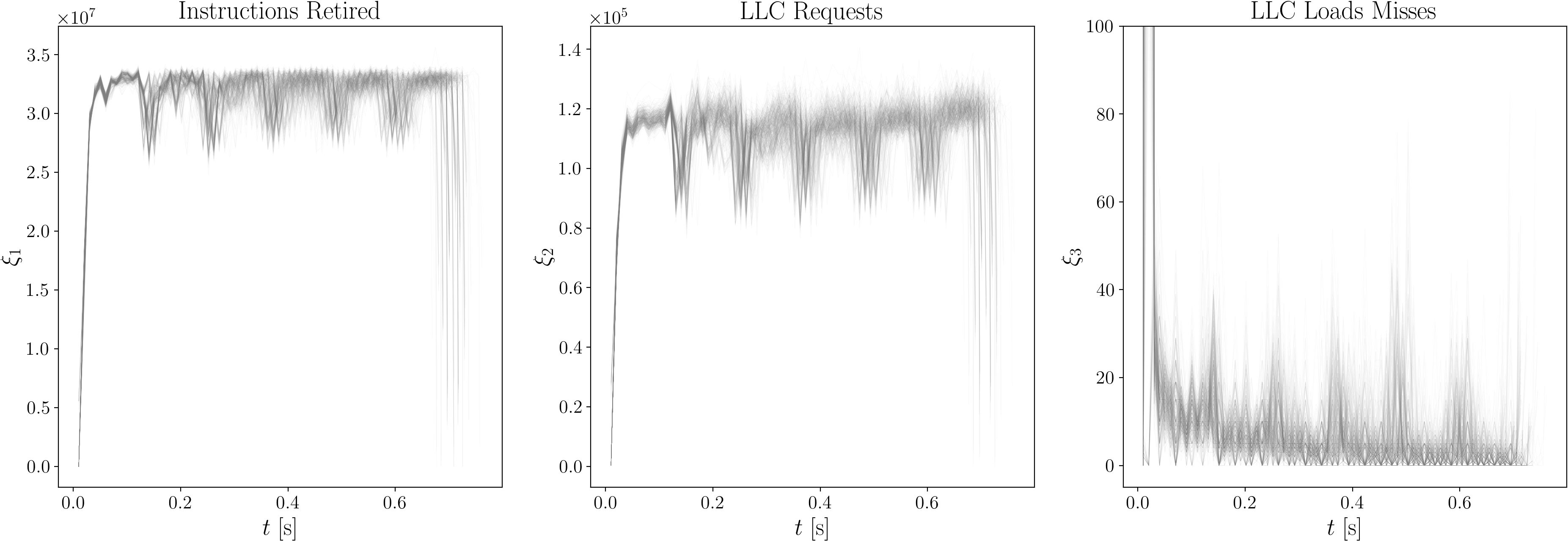
Refer to caption
Figure 5: Components of the measured feature vector 𝝃𝝃\bm{\xi} in (7) for the single core experiment in Sec. VI-A, for all of the five control cycles for 500 executions of the NMPC software, for a fixed cyber-physical context.

VI-A2 Numerical Results

To account for the asynchrony among the profiles, we analyzed the statistics of the control cycle end times, i.e., the (random) times needed to complete one pass of the NMPC feedback loop. For details, we refer the readers to [28, Table I, Fig. 4]. We then consider snapshots of the profiling data at times corresponding to the average control cycle end times as well as at sintsubscript𝑠ints_{\rm{int}} equi-spaced intervals between control cycles. This results in s=1+nc(sint+1)𝑠1subscript𝑛𝑐subscript𝑠int1s=1+n_{c}(s_{\rm{int}}+1) total marginals forming our path-structured MSBP (29), and completes Step 1 in section V-D.

Setting the regularizer ε=0.1𝜀0.1\varepsilon=0.1 and a numerical tolerance of 1014superscript101410^{-14}, we solve the discrete path-structured MSBP (29) with squared Euclidean cost 𝑪𝑪\bm{C} as in (39). Fig. 6 depicts the linear convergence of the Sinkhorn iterations (as in Proposition 3) shown w.r.t. the Hilbert metric (4). The path structure of the problem yields efficient computation of the Sinkhorn iterations leading to rapid convergence. In particular, setting sint:=4assignsubscript𝑠int4s_{\rm{int}}:=4 (and so s=26𝑠26s=26), we solve the MSBP (29) with ns=50026superscript𝑛𝑠superscript50026n^{s}=500^{26} decision variables in approx. 10s and 120absent120\approx 120 Sinkhorn iterations with no optimizations to the code. Notice that problems of this size are impractical to load in memory, let alone to solve efficiently using off-the-shelf solvers. This completes Step 2 in section V-D.

For Step 3, we compute sint+1=5subscript𝑠int15s_{\rm{int}}+1=5 distributional predictions μ^τ^σ^subscript^𝜇subscript^𝜏^𝜎\widehat{\mu}_{\widehat{\tau}_{\widehat{\sigma}}} at times τ^σ^subscript^𝜏^𝜎\widehat{\tau}_{\widehat{\sigma}}, temporally equispaced throughout the duration of the 3rd control cycle, i.e., between τ2(sint+1)+1subscript𝜏2subscript𝑠int11\tau_{2(s_{\rm{int}}+1)+1} and τ3(sint+1)+1subscript𝜏3subscript𝑠int11\tau_{3(s_{\rm{int}}+1)+1}, with

τ^σ^=τ2(sint+1)+1+(τ3(sint+1)+1τ2(sint+1)+1sint+2)σ^,subscript^𝜏^𝜎subscript𝜏2subscript𝑠int11subscript𝜏3subscript𝑠int11subscript𝜏2subscript𝑠int11subscript𝑠int2^𝜎\widehat{\tau}_{\widehat{\sigma}}=\tau_{2(s_{\rm{int}}+1)+1}+\Bigg{(}\frac{\tau_{3(s_{\rm{int}}+1)+1}-\tau_{2(s_{\rm{int}}+1)+1}}{s_{\rm{int}}+2}\Bigg{)}\widehat{\sigma},

where the index σ^sint+1\widehat{\sigma}\in\llbracket s_{\rm{int}}+1\rrbracket. Since τ^σ^[τ2(sint+1)+σ^,τ2(sint+1)+σ^+1]subscript^𝜏^𝜎subscript𝜏2subscript𝑠int1^𝜎subscript𝜏2subscript𝑠int1^𝜎1\widehat{\tau}_{\widehat{\sigma}}\in[\tau_{2(s_{\rm{int}}+1)+\widehat{\sigma}},\tau_{2(s_{\rm{int}}+1)+\widehat{\sigma}+1}], we used (38) with σ=2(sint+1)+σ^𝜎2subscript𝑠int1^𝜎\sigma=2(s_{\rm{int}}+1)+\widehat{\sigma} to arrive at the predictions. In Fig. 7, we compare our predictions against the observed empirical distributions.

Fig. 7 shows that our predictions capture the mode(s) of the measured distributions quite well. Further improvements can be made by placing marginals closer together in time. In this experiment, we do this by increasing the value of sintsubscript𝑠ints_{\rm{int}}, i.e., by placing more marginals equi-spaced between control cycle boundaries. In Table II, we report the Wasserstein distances W(,)𝑊W(\cdot,\cdot) as in (3) between the corresponding predicted and measured distributions:

Wσ^:=W(μ^τ^σ^,μτ^σ^)σ^sint+1.\displaystyle W_{\widehat{\sigma}}:=W(\widehat{\mu}_{\widehat{\tau}_{\widehat{\sigma}}},\mu_{\widehat{\tau}_{\widehat{\sigma}}})\quad\forall\widehat{\sigma}\in\llbracket s_{\rm{int}}+1\rrbracket. (57)

We computed (57) as the square roots of the optimal values of the corresponding Kantorovich linear programs [58, Ch. 3.1] that results from specializing (29) with s=2𝑠2s=2, ε=0𝜀0\varepsilon=0. As expected, placing the marginals closer together in time results in higher accuracy in predictions.
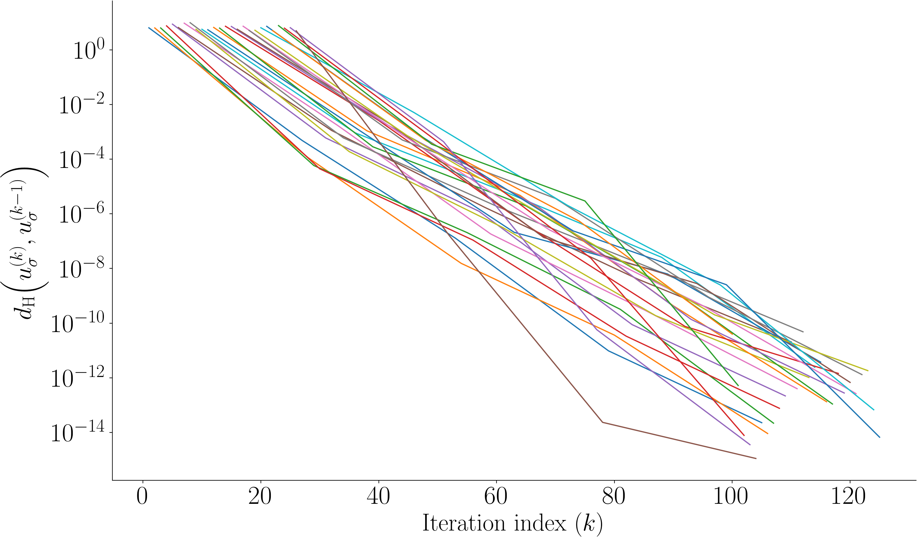
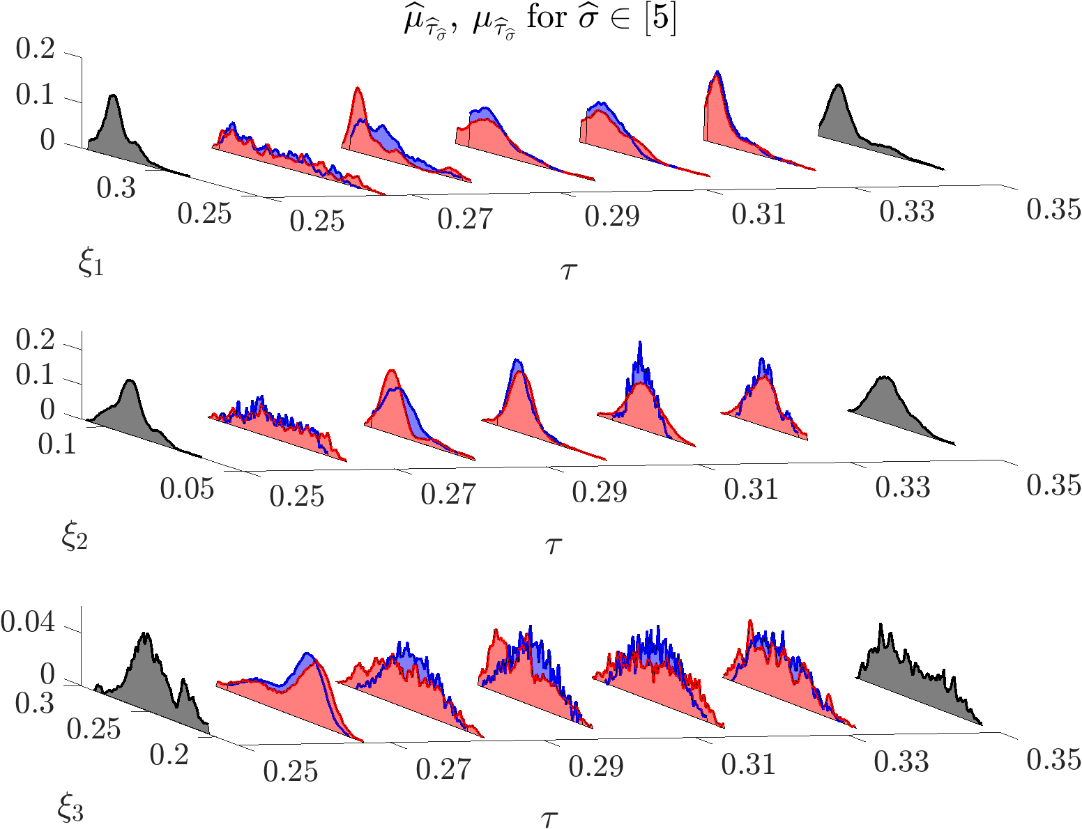
Refer to caption
Figure 6: Linear convergence of Sinkhorn iterations (36) for the single core experiment in Sec. VI-A, for sint=4subscript𝑠int4s_{\rm{int}}=4 w.r.t. the Hilbert’s projective metric dHsubscript𝑑Hd_{\rm{H}} in (4) between 𝒖σssubscript𝒖𝜎delimited-⟦⟧𝑠\bm{u}_{\sigma\in\llbracket s\rrbracket} at iteration indices k𝑘k and k1𝑘1k-1.
Refer to caption
Figure 7: Predicted μ^τ^σ^subscript^𝜇subscript^𝜏^𝜎\widehat{\mu}_{\widehat{\tau}_{\widehat{\sigma}}} (blue) vs. measured μτ^σ^subscript𝜇subscript^𝜏^𝜎\mu_{\widehat{\tau}_{\widehat{\sigma}}} (red) at times τ^σ^5subscript^𝜏^𝜎delimited-⟦⟧5\hat{\tau}_{\widehat{\sigma}\in\llbracket 5\rrbracket} for the single core experiment in Sec. VI-A, during the 3rd control cycle with sint=4subscript𝑠int4s_{\rm{int}}=4. Distributions at the control cycle boundaries are in black.
sintsubscript𝑠ints_{\rm{int}} W1subscript𝑊1W_{1} W2subscript𝑊2W_{2} W3subscript𝑊3W_{3} W4subscript𝑊4W_{4} W5subscript𝑊5W_{5}
00 2.049×1042.049superscript1042.049\times 10^{-4} - - - -
111 2.270×1042.270superscript1042.270\times 10^{-4} 1.175×1041.175superscript1041.175\times 10^{-4} - - -
222 5.772×1045.772superscript1045.772\times 10^{-4} 9.163×1059.163superscript1059.163\times 10^{-5} 3.794×1053.794superscript1053.794\times 10^{-5} - -
333 2.241×1042.241superscript1042.241\times 10^{-4} 1.643×1041.643superscript1041.643\times 10^{-4} 1.234×1041.234superscript1041.234\times 10^{-4} 6.010×1056.010superscript1056.010\times 10^{-5} -
444 6.372×1056.372superscript1056.372\times 10^{-5} 1.2691×1041.2691superscript1041.2691\times 10^{-4} 9.176×1059.176superscript1059.176\times 10^{-5} 6.689×1056.689superscript1056.689\times 10^{-5} 2.111×1052.111superscript1052.111\times 10^{-5}
TABLE II: For the single core experiment in Sec. VI-A, the number of intracycle marginals sintsubscript𝑠ints_{\rm{int}} vs. Wasserstein distances Wσ^subscript𝑊^𝜎W_{\widehat{\sigma}} as in (57).

VI-B Multi-core Experiment

For this experiment, we used the Canneal benchmark from the PARSEC suite [59]. Canneal is a resource-heavy, multi-threaded application that simulates an anneal workload to minimize routing costs for chip design. Specifically, Canneal pseudorandomly picks pairs of input elements to swap in a tight loop, leading to a heavy reliance on both cache and memory bandwidth. This can be seen in Fig. 8 where the average number of LLC misses decreases as the cache size increases. The dashed vertical lines represent the cache allocation used in our profiling.

VI-B1 Profiling

To enable multi-core profiling, we made a small modification to Canneal’s source code to pin each created thread to its own core. We then use perf, as with the single core experiment, to sample the computational resource state 𝝃jsuperscript𝝃𝑗\bm{\xi}^{j}, jJj\in\llbracket J\rrbracket, as in (7) for every 10 ms.

Desiring to examine how Canneal behaves when its resource allocation varies across its cores, we profile using a single context defined by J=4𝐽4J=4 cores, and resource allocations of (24,10,4,2)241042(24,10,4,2) MBs of LLC and (125,25,5,1)1252551(125,25,5,1) MBps of memory bandwidth, ordered left-to-right by increasing CPU number. So, CPU 1 has the highest resource allocation while CPU 4 has the lowest. For this choice of context, we collected a total of n=400𝑛400n=400 profiles for the Canneal software; these profiles are shown in Fig. 9. For the barycentric formulation, we fix n0=600subscript𝑛0600n_{0}=600.

Refer to caption
Figure 8: LLC miss rate per cache size for the Canneal benchmark in Sec. VI-A. The dashed vertical lines show our resource allocations per core.
Refer to caption
Figure 9: Components of 𝝃jsuperscript𝝃𝑗\bm{\xi}^{j}, j4j\in\llbracket 4\rrbracket, for the n=400𝑛400n=400 executions of the Canneal benchmark in Sec. VI-B, for all CPUs. Observe the erratic behavior of CPU4, which has the least hardware resources, as well that of CPU1, which has the most.

VI-B2 Numerical Results

We placed snapshots at times τσ{0.0,0.5,1.5,2.5,5.0,9.5,10.5}subscript𝜏𝜎0.00.51.52.55.09.510.5\tau_{\sigma}\in\{0.0,0.5,1.5,2.5,5.0,9.5,10.5\} (so s=7𝑠7s=7) and interpolated at times τ^σ^{0.8,2.2,7.0,9.0,10.0}subscript^𝜏^𝜎0.82.27.09.010.0\widehat{\tau}_{\widehat{\sigma}}\in\{0.8,2.2,7.0,9.0,10.0\} (so σ^5\widehat{\sigma}\in\llbracket 5\rrbracket). Both BC and SP methods were then used to solve the MSBPs (31) and (33) respectively, therefrom we used (38) to estimate the resource usage distributions at the desired times.

Remark 7.

For this experiment, our choice of marginals and interpolation times was made primarily for the sake of presentability – it would certainly be feasible to naïvely partition the profiles into equispaced intervals and place marginals at their boundaries, and to interpolate at will. As discussed in Sec. VI-B for the single-core experiment, placing more of these marginals temporally closer together would result in more accurate predictions.

Once again, the code for solution of (31) and (33), including the computation of the projections in Propositions 5 and 6, were implemented in MATLAB with some minor optimizations owing to the large size of the problem (the BC and SP formulations have 40035superscript40035400^{35} and 40022superscript40022400^{22} decision variables respectively; see Sec. V).

With the regularizer ε=0.05𝜀0.05\varepsilon=0.05 and a numerical tolerance of 1013superscript101310^{-13}, the BC and SP algorithms converged in 0.48100.48100.4810s and 0.50550.50550.5055s, with 110110110 and 127127127 iterations respectively (see Fig. 10). The predicted distributions, marginalized to each component of 𝝃jsuperscript𝝃𝑗\bm{\xi}^{j}, jJj\in\llbracket J\rrbracket, are shown in Fig. 11. Finally, Table III compares the Wasserstein distances of the predicted distributions for each CPU from those measured from our profiles, i.e.,

Wσ^j:=W(μ^τ^σ^j,μτ^σ^j)(j,σ^)J×sint+1.\displaystyle W_{\widehat{\sigma}}^{j}:=W(\widehat{\mu}_{\widehat{\tau}_{\widehat{\sigma}}}^{j},\mu_{\widehat{\tau}_{\widehat{\sigma}}}^{j})\quad\forall(j,\widehat{\sigma})\in\llbracket J\rrbracket\times\llbracket s_{\rm{int}}+1\rrbracket. (58)

These figures show the same behavior as in the single-core experiment – primarily, that our predictions accurately capture the mode(s) of the resource usage distribution at all interpolation times. Note that at σ^=1,τ^σ^=0.8formulae-sequence^𝜎1subscript^𝜏^𝜎0.8\widehat{\sigma}=1,\>\widehat{\tau}_{\widehat{\sigma}}=0.8, all CPUs except the CPU 1 are idle. Our predictions match the measured distribution exactly for the CPUs 2, 3, and 4 (i.e. the Dirac delta at 00 for all components), but not so for CPU 1, which has a nontrivial distribution.
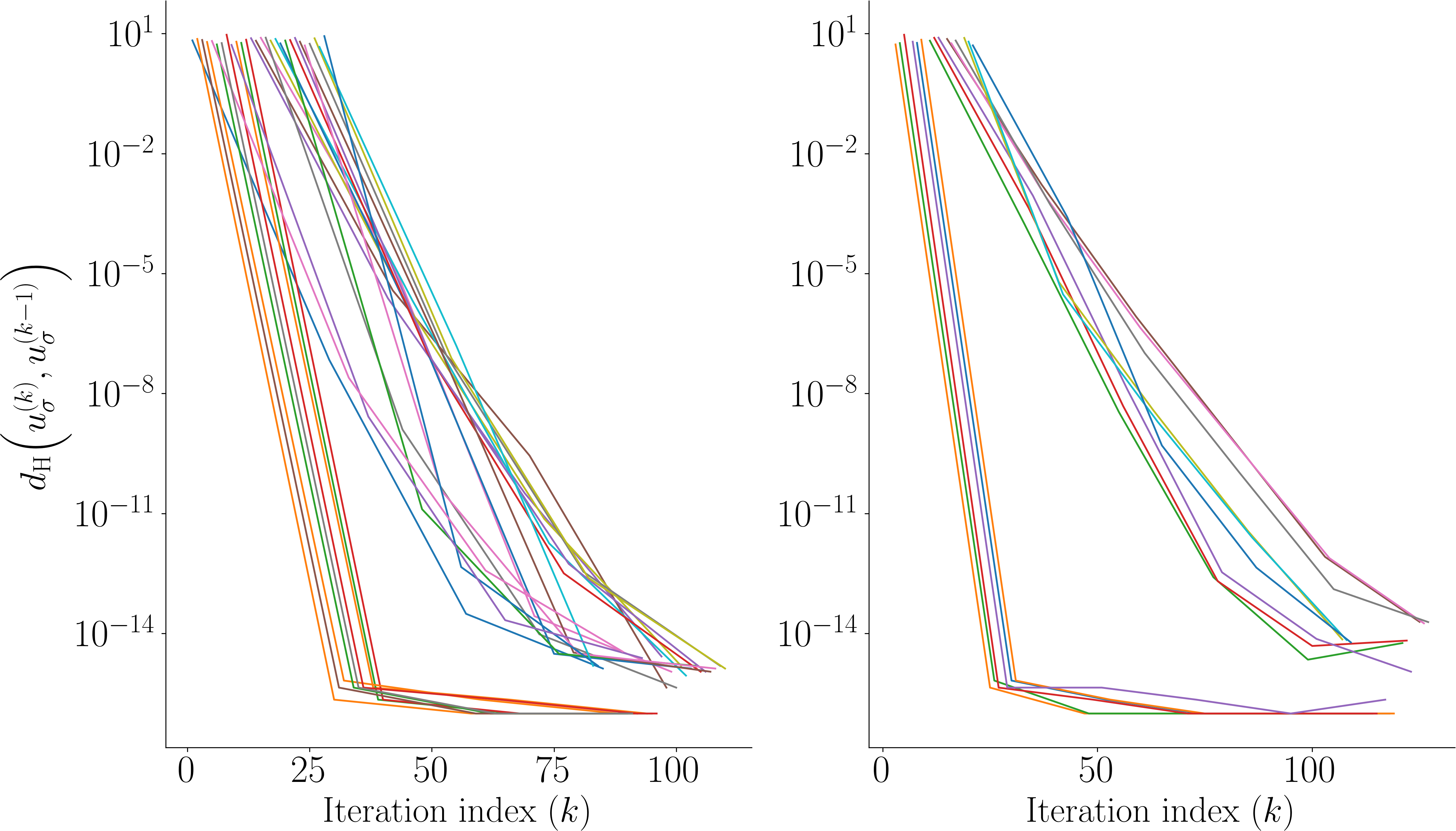
Refer to caption
Figure 10: Convergence of Sinkhorn iterations of both BC (left) and SP (right) algorithms for the Canneal benchmark in Sec. VI-B, shown w.r.t. the Hilbert projective metric dHsubscript𝑑Hd_{\rm{H}} as in (4).
Refer to caption
Refer to caption
Refer to caption
Refer to caption
Figure 11: Resource usage distributions predicted with the BC structure (red), the SP structure (blue), vs. the measured distributions (grey) at prediction times τ^σ^5\widehat{\tau}_{\widehat{\sigma}}\in\llbracket 5\rrbracket for the multi-core Canneal benchmark in Sec. VI-B.
j𝑗j W1jsuperscriptsubscript𝑊1𝑗W_{1}^{j} W2jsuperscriptsubscript𝑊2𝑗W_{2}^{j} W3jsuperscriptsubscript𝑊3𝑗W_{3}^{j} W4jsuperscriptsubscript𝑊4𝑗W_{4}^{j} W5jsuperscriptsubscript𝑊5𝑗W_{5}^{j}
111 4.077×1054.077superscript1054.077\times 10^{-5} 1.009×1071.009superscript1071.009\times 10^{-7} 2.131×1072.131superscript1072.131\times 10^{-7} 1.976×1071.976superscript1071.976\times 10^{-7} 1.509×1071.509superscript1071.509\times 10^{-7}
222 00 1.135×1071.135superscript1071.135\times 10^{-7} 2.342×1072.342superscript1072.342\times 10^{-7} 7.684×1087.684superscript1087.684\times 10^{-8} 8.805×1088.805superscript1088.805\times 10^{-8}
333 00 1.149×1071.149superscript1071.149\times 10^{-7} 1.534×1071.534superscript1071.534\times 10^{-7} 5.752×1085.752superscript1085.752\times 10^{-8} 6.538×1086.538superscript1086.538\times 10^{-8}
444 00 3.647×1083.647superscript1083.647\times 10^{-8} 2.146×1072.146superscript1072.146\times 10^{-7} 1.906×1071.906superscript1071.906\times 10^{-7} 9.713×1089.713superscript1089.713\times 10^{-8}


j𝑗j W1jsuperscriptsubscript𝑊1𝑗W_{1}^{j} W2jsuperscriptsubscript𝑊2𝑗W_{2}^{j} W3jsuperscriptsubscript𝑊3𝑗W_{3}^{j} W4jsuperscriptsubscript𝑊4𝑗W_{4}^{j} W5jsuperscriptsubscript𝑊5𝑗W_{5}^{j}
111 4.079×1054.079superscript1054.079\times 10^{-5} 1.062×1071.062superscript1071.062\times 10^{-7} 2.173×1072.173superscript1072.173\times 10^{-7} 2.110×1072.110superscript1072.110\times 10^{-7} 1.575×1071.575superscript1071.575\times 10^{-7}
222 00 1.048×1071.048superscript1071.048\times 10^{-7} 2.333×1072.333superscript1072.333\times 10^{-7} 7.303×1087.303superscript1087.303\times 10^{-8} 9.186×1089.186superscript1089.186\times 10^{-8}
333 00 1.065×1071.065superscript1071.065\times 10^{-7} 1.576×1071.576superscript1071.576\times 10^{-7} 6.394×1086.394superscript1086.394\times 10^{-8} 6.935×1086.935superscript1086.935\times 10^{-8}
444 00 5.553×1085.553superscript1085.553\times 10^{-8} 2.269×1072.269superscript1072.269\times 10^{-7} 1.857×1071.857superscript1071.857\times 10^{-7} 9.691×1089.691superscript1089.691\times 10^{-8}
TABLE III: Wasserstein distances (58) between the measured distributions and those predicted in the BC case (top) and SP case (bottom) for the Canneal benchmark in Sec. VI-B at each τ^σ^5subscript^𝜏^𝜎delimited-⟦⟧5\hat{\tau}_{\widehat{\sigma}\in\llbracket 5\rrbracket}.

VII Conclusions

This work explores a new vision for learning and predicting stochastic time-varying computational resource usage from hardware-software profile data in both single and multi-core platforms. We propose to formulate the problem as a distributional learning problem directly in the joint space of correlated computational resources such as processor availability, memory bandwidth, etc. This leads to graph-structured multi-marginal Schrödinger bridge problems (MSBPs) where the specific graph structures are induced by underlying single or multi-core nature of computation. At first glance, such formulations for scattered profile data appear computationally intractable because they involve tensorial convex optimization problems where the number of primal variables is exponential in the number of observational snapshots. By leveraging strong duality and graph structures, we show that the computational complexities can be reduced from exponential to linear without approximation, and these problems can in fact be solved efficiently via nonparametric computation with maximum likelihood guarantees in the space of distributions. This enables us to predict the most likely joint (and hence all marginal) computational resource usage distribution at any user-specified query time. We emphasize that our proposed algorithms and the benchmark results reported here, directly work with the scattered profile data without gridding the joint space of computational resource (here, instructions retired, LLC requests, LLC load misses). For the single core case, we illustrate the computational details for a nonlinear model predictive controller benchmark. For the multi-core case, we provide the results for a benchmark software from real-time systems literature.

We expect the proposed learning framework to be of interest to both control and real-time systems community because it opens the door for fine-grained dynamic scheduler design, especially for resource-constrained environments such as controlled cyber-physical systems. The learning-scheduling co-design that builds on the proposed method, will comprise our future work. Another direction of interest is to account for the asynchronous nature of the profiles by formulating the corresponding MSBPs with joint space-time stochasticity, i.e., as distributional generalization of optimal stopping problems initiated in the recent work [60].

-A Proof of Proposition 5

With 𝑲𝑲\bm{K} as in (44) and 𝑼𝑼\bm{U} as in (35b), consider the Hilbert-Schmidt inner product

𝐊,𝐔=i(r,),(r,)ΛBC[𝑲(i(r,)(r,)ΛBC)][𝑼(i(r,)(r,)ΛBC)]𝐊𝐔subscriptsubscript𝑖𝑟𝑟subscriptΛBCdelimited-[]subscript𝑲conditionalsubscript𝑖𝑟𝑟subscriptΛBCdelimited-[]subscript𝑼conditionalsubscript𝑖𝑟𝑟subscriptΛBC\displaystyle\langle\mathbf{K},\mathbf{U}\rangle=\sum_{\begin{subarray}{c}i_{(r,\ell)},\\ (r,\ell)\in\Lambda_{\rm{BC}}\end{subarray}}\left[\bm{K}_{(i_{(r,\ell)}\mid(r,\ell)\in\Lambda_{\rm{BC}})}\right]\left[\bm{U}_{(i_{(r,\ell)}\mid(r,\ell)\in\Lambda_{\rm{BC}})}\right]
=i(r,),(r,)ΛBC((σ=1s1[Ki(0,σ),i(0,σ+1)0,σ])\displaystyle=\sum_{\begin{subarray}{c}i_{(r,\ell)},\\ (r,\ell)\in\Lambda_{\rm{BC}}\end{subarray}}\Bigg{(}\bigg{(}\prod_{\sigma=1}^{s-1}\left[K_{i_{(0,\sigma)},i_{(0,\sigma+1)}}^{0,\sigma}\right]\bigg{)}
(σ=1sj=1J[Ki(j,σ),i(0,σ)j,σ])(σ=1sj=0J[(𝒖σj)i(j,σ)]))\displaystyle\quad\quad\quad\bigg{(}\prod_{\sigma=1}^{s}\prod_{j=1}^{J}\left[K_{i_{(j,\sigma)},i_{(0,\sigma)}}^{j,\sigma}\right]\bigg{)}\bigg{(}\prod_{\sigma=1}^{s}\prod_{j=0}^{J}\left[(\bm{u}_{\sigma}^{j})_{i_{(j,\sigma)}}\right]\bigg{)}\Bigg{)}
=i(0,),si(r,),(r,)J×s((σ=1s1[Ki(0,σ),i(0,σ+1)0,σ])\displaystyle=\sum_{\begin{subarray}{c}i_{(0,\ell)},\\ \ell\in\llbracket s\rrbracket\end{subarray}}\sum_{\begin{subarray}{c}i_{(r,\ell)},\\ (r,\ell)\in\llbracket J\rrbracket\times\llbracket s\rrbracket\end{subarray}}\Bigg{(}\bigg{(}\prod_{\sigma=1}^{s-1}\left[K_{i_{(0,\sigma)},i_{(0,\sigma+1)}}^{0,\sigma}\right]\bigg{)}
σ=1s(j=1J[Ki(j,σ),i(0,σ)j,σ])(j=0J[(𝒖σj)i(j,σ)]))\displaystyle\quad\quad\quad\prod_{\sigma=1}^{s}\bigg{(}\prod_{j=1}^{J}\left[K_{i_{(j,\sigma)},i_{(0,\sigma)}}^{j,\sigma}\right]\bigg{)}\bigg{(}\prod_{j=0}^{J}\left[(\bm{u}_{\sigma}^{j})_{i_{(j,\sigma)}}\right]\bigg{)}\Bigg{)}
=i(0,),s((σ=1s1[Ki(0,σ),i(0,σ+1)0,σ])\displaystyle=\sum_{\begin{subarray}{c}i_{(0,\ell)},\>\ell\in\llbracket s\rrbracket\end{subarray}}\Bigg{(}\bigg{(}\prod_{\sigma=1}^{s-1}\left[K_{i_{(0,\sigma)},i_{(0,\sigma+1)}}^{0,\sigma}\right]\bigg{)}
σ=1si(r,),(r,)J×s(j=1J[Ki(j,σ),i(0,σ)j,σ])(j=0J[(𝒖σj)i(j,σ)]))\displaystyle\prod_{\sigma=1}^{s}\sum_{\begin{subarray}{c}i_{(r,\ell)},\\ (r,\ell)\in\llbracket J\rrbracket\times\llbracket s\rrbracket\end{subarray}}\bigg{(}\prod_{j=1}^{J}\left[K_{i_{(j,\sigma)},i_{(0,\sigma)}}^{j,\sigma}\right]\bigg{)}\bigg{(}\prod_{j=0}^{J}\left[(\bm{u}_{\sigma}^{j})_{i_{(j,\sigma)}}\right]\bigg{)}\Bigg{)}
=i(0,),s((σ=1s1[Ki(0,σ),i(0,σ+1)0,σ])\displaystyle=\sum_{\begin{subarray}{c}i_{(0,\ell)},\>\ell\in\llbracket s\rrbracket\end{subarray}}\Bigg{(}\bigg{(}\prod_{\sigma=1}^{s-1}\left[K_{i_{(0,\sigma)},i_{(0,\sigma+1)}}^{0,\sigma}\right]\bigg{)}
σ=1s[(𝒖σ0(j=1JKj,σ𝒖σj):=𝒑σ)i(0,σ)])\displaystyle\quad\quad\quad\quad\prod_{\sigma=1}^{s}\bigg{[}\bigg{(}\underbrace{\bm{u}_{\sigma}^{0}\odot\Big{(}\bigodot_{j=1}^{J}K^{j,\sigma}\bm{u}_{\sigma}^{j}\Big{)}}_{:=\bm{p}_{\sigma}}\bigg{)}_{i_{(0,\sigma)}}\bigg{]}\Bigg{)}
=𝒑1(σ=2s1K0,σ1diag(𝒑σ))K0,s1𝒑sabsentsuperscriptsubscript𝒑1topsuperscriptsubscriptproduct𝜎2𝑠1superscript𝐾0𝜎1diagsubscript𝒑𝜎superscript𝐾0𝑠1subscript𝒑𝑠\displaystyle=\bm{p}_{1}^{\top}\bigg{(}\prod_{\sigma=2}^{s-1}K^{0,\sigma-1}\mathrm{diag}(\bm{p}_{\sigma})\bigg{)}K^{0,s-1}\bm{p}_{s} (59)
=𝒑1(m=2σ1K0,m1diag(𝒑m))K0,σ1absentsuperscriptsubscript𝒑1topsuperscriptsubscriptproduct𝑚2𝜎1superscript𝐾0𝑚1diagsubscript𝒑𝑚superscript𝐾0𝜎1\displaystyle=\bm{p}_{1}^{\top}\bigg{(}\prod_{m=2}^{\sigma-1}K^{0,m-1}\mathrm{diag}(\bm{p}_{m})\bigg{)}K^{0,\sigma-1}
diag(𝒖σ0(j=1JKj,σ𝒖σj))absentdiagdirect-productsuperscriptsubscript𝒖𝜎0superscriptsubscript𝑗1𝐽superscript𝐾𝑗𝜎superscriptsubscript𝒖𝜎𝑗\displaystyle\quad\quad\quad\cdot\mathrm{diag}\bigg{(}\bm{u}_{\sigma}^{0}\odot\Big{(}\bigodot_{j=1}^{J}K^{j,\sigma}\bm{u}_{\sigma}^{j}\Big{)}\bigg{)}
(m=σ+1s1K0,m1diag(𝒑m))K0,s1𝒑sabsentsuperscriptsubscriptproduct𝑚𝜎1𝑠1superscript𝐾0𝑚1diagsubscript𝒑𝑚superscript𝐾0𝑠1subscript𝒑𝑠\displaystyle\quad\quad\quad\quad\quad\quad\cdot\bigg{(}\prod_{m=\sigma+1}^{s-1}K^{0,m-1}\mathrm{diag}(\bm{p}_{m})\bigg{)}K^{0,s-1}\bm{p}_{s} (60)

where (59) follows by the same argument as for Proposition 4 (see also [28, Proposition 1]). Then the unimarginal projections (45a)-(45b) follow by applying Lemma 2 to (60).

For the bimarginal projections, let (j,σ)J×s(j,\sigma)\in\llbracket J\rrbracket\times\llbracket s\rrbracket and σ1,σ2s\sigma_{1},\sigma_{2}\in\llbracket s\rrbracket such that σ1<σ2subscript𝜎1subscript𝜎2\sigma_{1}<\sigma_{2}. Starting with (59), we have

𝐊,𝐔=𝒑1(σ=2s1K0,σ1diag(𝒑σ))K0,s1𝒑s𝐊𝐔superscriptsubscript𝒑1topsuperscriptsubscriptproduct𝜎2𝑠1superscript𝐾0𝜎1diagsubscript𝒑𝜎superscript𝐾0𝑠1subscript𝒑𝑠\displaystyle\langle\mathbf{K},\mathbf{U}\rangle=\bm{p}_{1}^{\top}\bigg{(}\prod_{\sigma=2}^{s-1}K^{0,\sigma-1}\mathrm{diag}(\bm{p}_{\sigma})\bigg{)}K^{0,s-1}\bm{p}_{s}
=𝒑1(m=2sK0,m1𝒑m)absentsuperscriptsubscript𝒑1topsuperscriptsubscript𝑚2𝑠superscript𝐾0𝑚1subscript𝒑𝑚\displaystyle=\bm{p}_{1}^{\top}\bigg{(}\bigodot_{m=2}^{s}K^{0,m-1}\bm{p}_{m}\bigg{)}
=𝟏diag(𝒑σ)K0,σ1(𝒑1m=2,mσsK0,m1𝒑m)absentsuperscript1topdiagsubscript𝒑𝜎superscriptsuperscript𝐾0𝜎1topdirect-productsubscript𝒑1superscriptsubscript𝑚2𝑚𝜎𝑠superscript𝐾0𝑚1subscript𝒑𝑚\displaystyle=\bm{1}^{\top}\mathrm{diag}(\bm{p}_{\sigma}){K^{0,\sigma-1}}^{\top}\bigg{(}\bm{p}_{1}\odot\bigodot_{\begin{subarray}{c}m=2,\\ m\neq\sigma\end{subarray}}^{s}K^{0,m-1}\bm{p}_{m}\bigg{)}
=𝟏diag(𝒖σ0(k=1JKk,σ𝒖σk))absentsuperscript1topdiagdirect-productsuperscriptsubscript𝒖𝜎0superscriptsubscript𝑘1𝐽superscript𝐾𝑘𝜎superscriptsubscript𝒖𝜎𝑘\displaystyle=\bm{1}^{\top}\mathrm{diag}\bigg{(}\bm{u}_{\sigma}^{0}\odot\Big{(}\bigodot_{k=1}^{J}K^{k,\sigma}\bm{u}_{\sigma}^{k}\Big{)}\bigg{)}
K0,σ1(𝒑1m=2,mσsK0,m1𝒑m)superscriptsuperscript𝐾0𝜎1topdirect-productsubscript𝒑1superscriptsubscript𝑚2𝑚𝜎𝑠superscript𝐾0𝑚1subscript𝒑𝑚\displaystyle\quad\quad\quad\quad\quad\quad{K^{0,\sigma-1}}^{\top}\bigg{(}\bm{p}_{1}\odot\bigodot_{\begin{subarray}{c}m=2,\\ m\neq\sigma\end{subarray}}^{s}K^{0,m-1}\bm{p}_{m}\bigg{)}
=𝟏diag(𝒖σ0)diag(k=1kjJKk,σ𝒖σk)absentsuperscript1topdiagsuperscriptsubscript𝒖𝜎0diagsuperscriptsubscript𝑘1𝑘𝑗𝐽superscript𝐾𝑘𝜎superscriptsubscript𝒖𝜎𝑘\displaystyle=\bm{1}^{\top}\mathrm{diag}(\bm{u}_{\sigma}^{0})\mathrm{diag}\bigg{(}\bigodot_{\begin{subarray}{c}k=1\\ k\neq j\end{subarray}}^{J}K^{k,\sigma}\bm{u}_{\sigma}^{k}\bigg{)}
diag(K0,σ1(𝒑1m=2,mσsK0,m1𝒑m))Kj,σdiag(𝒖σj)𝟏diagsuperscriptsuperscript𝐾0𝜎1topdirect-productsubscript𝒑1superscriptsubscript𝑚2𝑚𝜎𝑠superscript𝐾0𝑚1subscript𝒑𝑚superscript𝐾𝑗𝜎diagsuperscriptsubscript𝒖𝜎𝑗1\displaystyle\quad\mathrm{diag}\Bigg{(}{K^{0,\sigma-1}}^{\top}\bigg{(}\bm{p}_{1}\odot\bigodot_{\begin{subarray}{c}m=2,\\ m\neq\sigma\end{subarray}}^{s}K^{0,m-1}\bm{p}_{m}\bigg{)}\Bigg{)}K^{j,\sigma}\mathrm{diag}(\bm{u}_{\sigma}^{j})\bm{1}
=𝟏diag(𝒖σ0)absentsuperscript1topdiagsuperscriptsubscript𝒖𝜎0\displaystyle=\bm{1}^{\top}\mathrm{diag}(\bm{u}_{\sigma}^{0})
diag(K0,σ1(𝒑1(m=2,mσsK0,m1𝒑m)(k=1kjJKk,σ𝒖σk))=:𝝆(0,σ),(j,σ))diagsuperscriptsuperscript𝐾0𝜎1topsubscriptdirect-productsubscript𝒑1superscriptsubscript𝑚2𝑚𝜎𝑠superscript𝐾0𝑚1subscript𝒑𝑚superscriptsubscript𝑘1𝑘𝑗𝐽superscript𝐾𝑘𝜎superscriptsubscript𝒖𝜎𝑘:absentsubscript𝝆0𝜎𝑗𝜎\displaystyle\mathrm{diag}\Bigg{(}{K^{0,\sigma-1}}^{\top}\underbrace{\bigg{(}\bm{p}_{1}\odot\Big{(}\bigodot_{\begin{subarray}{c}m=2,\\ m\neq\sigma\end{subarray}}^{s}K^{0,m-1}\bm{p}_{m}\Big{)}\Big{(}\bigodot_{\begin{subarray}{c}k=1\\ k\neq j\end{subarray}}^{J}K^{k,\sigma}\bm{u}_{\sigma}^{k}\Big{)}\bigg{)}}_{=:\bm{\rho}_{(0,\sigma),(j,\sigma)}}\Bigg{)}
Kj,σdiag(𝒖σj)𝟏superscript𝐾𝑗𝜎diagsuperscriptsubscript𝒖𝜎𝑗1\displaystyle\quad\quad\quad\quad K^{j,\sigma}\mathrm{diag}(\bm{u}_{\sigma}^{j})\bm{1} (61)
=(𝒑1K0,1k=2σ11diag(𝒑k)K0,k)absentsuperscriptsubscript𝒑1topsuperscript𝐾01superscriptsubscriptproduct𝑘2subscript𝜎11diagsubscript𝒑𝑘superscript𝐾0𝑘\displaystyle=\bigg{(}\bm{p}_{1}^{\top}K^{0,1}\prod_{k=2}^{\sigma_{1}-1}\mathrm{diag}(\bm{p}_{k})K^{0,k}\bigg{)}
diag(𝒑σ1)(k=σ1+1σ21K0,k1diag(𝒑k))K0,σ21diag(𝒑σ2)absentdiagsubscript𝒑subscript𝜎1superscriptsubscriptproduct𝑘subscript𝜎11subscript𝜎21superscript𝐾0𝑘1diagsubscript𝒑𝑘superscript𝐾0subscript𝜎21diagsubscript𝒑subscript𝜎2\displaystyle\quad\cdot\mathrm{diag}(\bm{p}_{\sigma_{1}})\bigg{(}\prod_{k=\sigma_{1}+1}^{\sigma_{2}-1}K^{0,k-1}\mathrm{diag}(\bm{p}_{k})\bigg{)}K^{0,\sigma_{2}-1}\mathrm{diag}(\bm{p}_{\sigma_{2}})
(k=σ2+1s1K0,k1diag(𝒑k))K0,s1𝒑s.absentsuperscriptsubscriptproduct𝑘subscript𝜎21𝑠1superscript𝐾0𝑘1diagsubscript𝒑𝑘superscript𝐾0𝑠1subscript𝒑𝑠\displaystyle\quad\cdot\bigg{(}\prod_{k=\sigma_{2}+1}^{s-1}K^{0,k-1}\mathrm{diag}(\bm{p}_{k})\bigg{)}K^{0,s-1}\bm{p}_{s}. (62)

Then, (46a) follows from (61), and (46b) follows from expanding diag(𝒑σ1)diagsubscript𝒑subscript𝜎1\mathrm{diag}(\bm{p}_{\sigma_{1}}) and diag(𝒑σ2)diagsubscript𝒑subscript𝜎2\mathrm{diag}(\bm{p}_{\sigma_{2}}) in (62), followed by the application of Lemma 2. \blacksquare

-B Proof of Proposition 6

With 𝑲𝑲\bm{K} as in (51) and 𝑼𝑼\bm{U} as in (35b), we start with the Hilbert-Schmidt inner product

𝐊,𝐔=i(j,σ),(j,σ)ΛSP[𝑲(i(j,σ)(j,σ)ΛSP)][𝑼(i(j,σ)(j,σ)ΛSP)]𝐊𝐔subscriptsubscript𝑖𝑗𝜎𝑗𝜎subscriptΛSPdelimited-[]subscript𝑲conditionalsubscript𝑖𝑗𝜎𝑗𝜎subscriptΛSPdelimited-[]subscript𝑼conditionalsubscript𝑖𝑗𝜎𝑗𝜎subscriptΛSP\displaystyle\langle\mathbf{K},\mathbf{U}\rangle=\sum_{\begin{subarray}{c}i_{(j,\sigma)},\\ (j,\sigma)\in\Lambda_{\rm{SP}}\end{subarray}}\left[\bm{K}_{(i_{(j,\sigma)}\mid(j,\sigma)\in\Lambda_{\rm{SP}})}\right]\left[\bm{U}_{(i_{(j,\sigma)}\mid(j,\sigma)\in\Lambda_{\rm{SP}})}\right]
=i(j,σ),(j,σ)ΛSP(k=1J[𝑲i(1,1),(i(j,σ)(j,σ)ΛSPk),i(1,s)k])absentsubscriptsubscript𝑖𝑗𝜎𝑗𝜎subscriptΛSPsuperscriptsubscriptproduct𝑘1𝐽delimited-[]superscriptsubscript𝑲subscript𝑖11conditionalsubscript𝑖𝑗𝜎𝑗𝜎superscriptsubscriptΛSP𝑘subscript𝑖1𝑠𝑘\displaystyle=\sum_{i_{(j,\sigma)},(j,\sigma)\in\Lambda_{\rm{SP}}}\left(\prod_{k=1}^{J}\left[\bm{K}_{i_{(1,1)},(i_{(j,\sigma)}\mid(j,\sigma)\in\Lambda_{\rm{SP}}^{k}),i_{(1,s)}}^{k}\right]\right)
(𝒖11)i(1,1)(k=1Jσ=2s1(𝒖σk)i(k,σ))(𝒖s1)i(1,s)subscriptsuperscriptsubscript𝒖11subscript𝑖11superscriptsubscriptproduct𝑘1𝐽superscriptsubscriptproduct𝜎2𝑠1subscriptsuperscriptsubscript𝒖𝜎𝑘subscript𝑖𝑘𝜎subscriptsuperscriptsubscript𝒖𝑠1subscript𝑖1𝑠\displaystyle\quad\quad\quad\quad(\bm{u}_{1}^{1})_{i_{(1,1)}}\Bigg{(}\prod_{k=1}^{J}\prod_{\sigma=2}^{s-1}(\bm{u}_{\sigma}^{k})_{i_{(k,\sigma)}}\Bigg{)}(\bm{u}_{s}^{1})_{i_{(1,s)}}
=𝒖11k=1J(Kk,1(σ=2s1diag(𝒖σk)Kk,σ):=Ak)𝒖s1absentsuperscriptsuperscriptsubscript𝒖11topsuperscriptsubscriptproduct𝑘1𝐽subscriptsuperscript𝐾𝑘1superscriptsubscriptproduct𝜎2𝑠1diagsuperscriptsubscript𝒖𝜎𝑘superscript𝐾𝑘𝜎assignabsentsubscript𝐴𝑘superscriptsubscript𝒖𝑠1\displaystyle={\bm{u}_{1}^{1}}^{\top}\prod_{k=1}^{J}\Bigg{(}\underbrace{K^{k,1}\left(\prod_{\sigma=2}^{s-1}\mathrm{diag}(\bm{u}_{\sigma}^{k})K^{k,\sigma}\right)}_{:=A_{k}}\Bigg{)}\bm{u}_{s}^{1} (63)
=𝒖11(k=1j1Ak)Aj(k=j+1JAk)(𝒖s1)absentsuperscriptsuperscriptsubscript𝒖11topsuperscriptsubscriptproduct𝑘1𝑗1subscript𝐴𝑘subscript𝐴𝑗superscriptsubscriptproduct𝑘𝑗1𝐽subscript𝐴𝑘superscriptsubscript𝒖𝑠1\displaystyle={\bm{u}_{1}^{1}}^{\top}\bigg{(}\prod_{k=1}^{j-1}A_{k}\bigg{)}A_{j}\bigg{(}\prod_{k=j+1}^{J}A_{k}\bigg{)}(\bm{u}_{s}^{1})
=𝒖11(k=1j1Ak)(Kj,1(m=2σ1diag(𝒖mj)Kj,m)𝒘1diag(𝒖σj)\displaystyle=\underbrace{{\bm{u}_{1}^{1}}^{\top}\bigg{(}\prod_{k=1}^{j-1}A_{k}\bigg{)}\Bigg{(}K^{j,1}\bigg{(}\prod_{m=2}^{\sigma-1}\mathrm{diag}(\bm{u}_{m}^{j})K^{j,m}\bigg{)}}_{\bm{w}_{1}^{\top}}\cdot\mathrm{diag}(\bm{u}_{\sigma}^{j})
Kj,σ(m=σ+1s1diag(𝒖mj)Kj,m))(k=j+1JAk)𝒖s1𝒘2\displaystyle\quad\cdot\underbrace{K^{j,\sigma}\bigg{(}\prod_{m=\sigma+1}^{s-1}\mathrm{diag}(\bm{u}_{m}^{j})K^{j,m}\bigg{)}\Bigg{)}\bigg{(}\prod_{k=j+1}^{J}A_{k}\bigg{)}\bm{u}_{s}^{1}}_{\bm{w}_{2}} (64)

wherefrom the projections (53a) and (53b) follow by applying Lemma 2 to (63). Similarly, (53c) follows by applying Lemma 2 to (64).

Next, for the bimarginal projections, we write

𝐊,𝐔=𝟏𝒘1diag(𝒖11)(k=1j1Ak)Kj,1Φdiag(𝒖2j)𝐊𝐔subscriptsuperscript1topsuperscriptsubscript𝒘1topdiagsuperscriptsubscript𝒖11subscriptsuperscriptsubscriptproduct𝑘1𝑗1subscript𝐴𝑘superscript𝐾𝑗1Φdiagsuperscriptsubscript𝒖2𝑗\displaystyle\langle\mathbf{K},\mathbf{U}\rangle=\underbrace{\mathbf{1}^{\top}}_{\bm{w}_{1}^{\top}}\cdot\mathrm{diag}(\bm{u}_{1}^{1})\cdot\underbrace{\bigg{(}\prod_{k=1}^{j-1}A_{k}\bigg{)}K^{j,1}}_{\Phi}\cdot\mathrm{diag}(\bm{u}_{2}^{j})
Kj,2(k=3s1diag(𝒖kj)Kj,k)(k=j+1JAk)𝒖s1𝒘3absentsubscriptsuperscript𝐾𝑗2superscriptsubscriptproduct𝑘3𝑠1diagsuperscriptsubscript𝒖𝑘𝑗superscript𝐾𝑗𝑘superscriptsubscriptproduct𝑘𝑗1𝐽subscript𝐴𝑘superscriptsubscript𝒖𝑠1subscript𝒘3\displaystyle\quad\cdot\underbrace{K^{j,2}\bigg{(}\prod_{k=3}^{s-1}\mathrm{diag}(\bm{u}_{k}^{j})K^{j,k}\bigg{)}\bigg{(}\prod_{k=j+1}^{J}A_{k}\bigg{)}\bm{u}_{s}^{1}}_{\bm{w}_{3}} (65)
=𝒖11(k=1j1Ak)Kj,1(k=2s2diag(𝒖kj)Kj,k)𝒘1absentsubscriptsuperscriptsuperscriptsubscript𝒖11topsuperscriptsubscriptproduct𝑘1𝑗1subscript𝐴𝑘superscript𝐾𝑗1superscriptsubscriptproduct𝑘2𝑠2diagsuperscriptsubscript𝒖𝑘𝑗superscript𝐾𝑗𝑘superscriptsubscript𝒘1top\displaystyle=\underbrace{{\bm{u}_{1}^{1}}^{\top}\bigg{(}\prod_{k=1}^{j-1}A_{k}\bigg{)}K^{j,1}\bigg{(}\prod_{k=2}^{s-2}\mathrm{diag}(\bm{u}_{k}^{j})K^{j,k}\bigg{)}}_{\bm{w}_{1}^{\top}}
diag(𝒖s1j)Kj,s1(k=j+1JAk)Φdiag(𝒖s1)𝟏𝒘3absentdiagsuperscriptsubscript𝒖𝑠1𝑗subscriptsuperscript𝐾𝑗𝑠1superscriptsubscriptproduct𝑘𝑗1𝐽subscript𝐴𝑘Φdiagsuperscriptsubscript𝒖𝑠1subscript1subscript𝒘3\displaystyle\quad\cdot\mathrm{diag}(\bm{u}_{s-1}^{j})\cdot\underbrace{K^{j,s-1}\bigg{(}\prod_{k=j+1}^{J}A_{k}\bigg{)}}_{\Phi}\cdot\mathrm{diag}(\bm{u}_{s}^{1})\cdot\underbrace{\mathbf{1}}_{\bm{w}_{3}} (66)
=𝒖11(k=1j1Ak)Kj,1(k=2σ1diag(𝒖kj)Kj,k)𝒘1diag(𝒖σj)absentsubscriptsuperscriptsuperscriptsubscript𝒖11topsuperscriptsubscriptproduct𝑘1𝑗1subscript𝐴𝑘superscript𝐾𝑗1superscriptsubscriptproduct𝑘2𝜎1diagsuperscriptsubscript𝒖𝑘𝑗superscript𝐾𝑗𝑘superscriptsubscript𝒘1topdiagsuperscriptsubscript𝒖𝜎𝑗\displaystyle=\underbrace{{\bm{u}_{1}^{1}}^{\top}\bigg{(}\prod_{k=1}^{j-1}A_{k}\bigg{)}K^{j,1}\bigg{(}\prod_{k=2}^{\sigma-1}\mathrm{diag}(\bm{u}_{k}^{j})K^{j,k}\bigg{)}}_{\bm{w}_{1}^{\top}}\cdot\mathrm{diag}(\bm{u}_{\sigma}^{j})
Kj,σΦdiag(𝒖σ+1j)absentsubscriptsuperscript𝐾𝑗𝜎Φdiagsuperscriptsubscript𝒖𝜎1𝑗\displaystyle\quad\cdot\underbrace{K^{j,\sigma}}_{\Phi}\cdot\mathrm{diag}(\bm{u}_{\sigma+1}^{j})
Kj,σ+1(j=σ+2s1diag(𝒖kj)Kj,k)(k=j+1JAk)𝒖s1𝒘3.absentsubscriptsuperscript𝐾𝑗𝜎1superscriptsubscriptproduct𝑗𝜎2𝑠1diagsuperscriptsubscript𝒖𝑘𝑗superscript𝐾𝑗𝑘superscriptsubscriptproduct𝑘𝑗1𝐽subscript𝐴𝑘superscriptsubscript𝒖𝑠1subscript𝒘3\displaystyle\cdot\underbrace{K^{j,\sigma+1}\Bigg{(}\prod_{j=\sigma+2}^{s-1}\mathrm{diag}(\bm{u}_{k}^{j})K^{j,k}\bigg{)}\bigg{(}\prod_{k=j+1}^{J}A_{k}\bigg{)}\bm{u}_{s}^{1}}_{\bm{w}_{3}}. (67)

Now (54a) follows from (65), (54b) from (66), and (54c) from (67). \blacksquare

References

  • [1] G. Bernat, A. Colin, and S. M. Petters, “WCET analysis of probabilistic hard real-time systems,” in RTSS, 2002.
  • [2] R. Wilhelm, J. Engblom, A. Ermedahl, N. Holsti, S. Thesing, D. Whalley, G. Bernat, C. Ferdinand, R. Heckmann, T. Mitra et al., “The worst-case execution-time problem—overview of methods and survey of tools,” ACM Transactions on Embedded Computing Systems (TECS), vol. 7, no. 3, pp. 1–53, 2008.
  • [3] R. I. Davis and A. Burns, “A survey of hard real-time scheduling for multiprocessor systems,” ACM computing surveys (CSUR), vol. 43, no. 4, pp. 1–44, 2011.
  • [4] S. J. Gil, I. Bate, G. Lima, L. Santinelli, A. Gogonel, and L. Cucu-Grosjean, “Open challenges for probabilistic measurement-based worst-case execution time,” IEEE Embedded Systems Letters, vol. 9, no. 3, pp. 69–72, 2017.
  • [5] L. Rüschendorf and L. Uckelmann, “On the n-coupling problem,” Journal of multivariate analysis, vol. 81, no. 2, pp. 242–258, 2002.
  • [6] B. Pass, “Multi-marginal optimal transport: theory and applications,” ESAIM: Mathematical Modelling and Numerical Analysis, vol. 49, no. 6, pp. 1771–1790, 2015.
  • [7] G. Buttazzo, L. De Pascale, and P. Gori-Giorgi, “Optimal-transport formulation of electronic density-functional theory,” Physical Review A, vol. 85, no. 6, p. 062502, 2012.
  • [8] C. Cotar, G. Friesecke, and C. Klüppelberg, “Density functional theory and optimal transportation with Coulomb cost,” Communications on Pure and Applied Mathematics, vol. 66, no. 4, pp. 548–599, 2013.
  • [9] G. Carlier, A. Oberman, and E. Oudet, “Numerical methods for matching for teams and wasserstein barycenters,” ESAIM: Mathematical Modelling and Numerical Analysis, vol. 49, no. 6, pp. 1621–1642, 2015.
  • [10] J.-D. Benamou, G. Carlier, and L. Nenna, “Generalized incompressible flows, multi-marginal transport and Sinkhorn algorithm,” Numerische Mathematik, vol. 142, pp. 33–54, 2019.
  • [11] H. Ennaji, Q. Mérigot, L. Nenna, and B. Pass, “Robust risk management via multi-marginal optimal transport,” Journal of Optimization Theory and Applications, pp. 1–28, 2024.
  • [12] F. Elvander, I. Haasler, A. Jakobsson, and J. Karlsson, “Multi-marginal optimal transport using partial information with applications in robust localization and sensor fusion,” Signal Processing, vol. 171, p. 107474, 2020.
  • [13] I. Haasler, A. Ringh, Y. Chen, and J. Karlsson, “Multimarginal optimal transport with a tree-structured cost and the Schrodinger bridge problem,” SIAM Journal on Control and Optimization, vol. 59, no. 4, pp. 2428–2453, 2021.
  • [14] M. Noble, V. De Bortoli, A. Doucet, and A. Durmus, “Tree-based diffusion Schrödinger bridge with applications to Wasserstein barycenters,” Advances in Neural Information Processing Systems, vol. 36, 2024.
  • [15] Y. Chen, T. T. Georgiou, and M. Pavon, “Stochastic control liaisons: Richard sinkhorn meets gaspard monge on a schrodinger bridge,” Siam Review, vol. 63, no. 2, pp. 249–313, 2021.
  • [16] A. M. Teter, Y. Chen, and A. Halder, “On the contraction coefficient of the Schrödinger bridge for stochastic linear systems,” IEEE Control Systems Letters, 2023.
  • [17] K. F. Caluya and A. Halder, “Finite horizon density steering for multi-input state feedback linearizable systems,” in ACC.   IEEE, 2020, pp. 3577–3582.
  • [18] K. F. Caluya and A. Halder, “Reflected Schrödinger bridge: Density control with path constraints,” in ACC.   IEEE, 2021, pp. 1137–1142.
  • [19] K. F. Caluya and A. Halder, “Wasserstein proximal algorithms for the Schrödinger bridge problem: Density control with nonlinear drift,” IEEE Transactions on Automatic Control, vol. 67, no. 3, pp. 1163–1178, 2021.
  • [20] I. Nodozi and A. Halder, “Schrödinger meets Kuramoto via Feynman-Kac: Minimum effort distribution steering for noisy nonuniform kuramoto oscillators,” in 2022 IEEE 61st Conference on Decision and Control (CDC).   IEEE, 2022, pp. 2953–2960.
  • [21] S. Haddad, A. Halder, and B. Singh, “Density-based stochastic reachability computation for occupancy prediction in automated driving,” IEEE Transactions on Control Systems Technology, vol. 30, no. 6, pp. 2406–2419, 2022.
  • [22] I. Nodozi, J. O’Leary, A. Mesbah, and A. Halder, “A physics-informed deep learning approach for minimum effort stochastic control of colloidal self-assembly,” in 2023 American Control Conference (ACC).   IEEE, 2023, pp. 609–615.
  • [23] M. Amiri and L. Mohammad-Khanli, “Survey on prediction models of applications for resources provisioning in cloud,” Journal of Network and Computer Applications, vol. 82, pp. 93–113, 2017.
  • [24] D. Saxena, J. Kumar, A. K. Singh, and S. Schmid, “Performance analysis of machine learning centered workload prediction models for cloud,” IEEE Transactions on Parallel and Distributed Systems, vol. 34, no. 4, pp. 1313–1330, 2023.
  • [25] V. Kumar, “Estimation of an early wcet using different machine learning approaches,” in Advances on P2P, Parallel, Grid, Cloud and Internet Computing, 2023, pp. 297–307.
  • [26] J. Lee, S. Y. Shin, S. Nejati, L. Briand, and Y. I. Parache, “Estimating probabilistic safe wcet ranges of real-time systems at design stages,” ACM Trans. Softw. Eng. Methodol., vol. 32, no. 2, mar 2023.
  • [27] K. Muts, “Multiobjective compiler-based optimizations for hard real-time systems,” Ph.D. dissertation, Technische Universität Hamburg, 2022.
  • [28] G. A. Bondar, R. Gifford, L. T. X. Phan, and A. Halder, “Path structured multimarginal Schrödinger bridge for probabilistic learning of hardware resource usage by control software,” 2023 American Control Conference, arXiv preprint arXiv:2310.00604, 2023.
  • [29] S. Warner, Modern algebra.   Courier Corporation, 1990.
  • [30] G. Birkhoff, “Extensions of Jentzsch’s theorem,” Transactions of the American Mathematical Society, vol. 85, no. 1, pp. 219–227, 1957.
  • [31] P. J. Bushell, “Hilbert’s metric and positive contraction mappings in a Banach space,” Archive for Rational Mechanics and Analysis, vol. 52, pp. 330–338, 1973.
  • [32] E. Kohlberg and J. W. Pratt, “The contraction mapping approach to the perron-frobenius theory: Why Hilbert’s metric?” Mathematics of Operations Research, vol. 7, no. 2, pp. 198–210, 1982.
  • [33] A. Dembo, Large deviations techniques and applications.   Springer Science & Business Media, 2009.
  • [34] E. Schrödinger, Über die umkehrung der naturgesetze.   Verlag der Akademie der Wissenschaften in Kommission bei Walter De Gruyter u. Company., 1931.
  • [35] E. Schrödinger, “Sur la théorie relativiste de l’électron et l’interprétation de la mécanique quantique,” in Annales de l’institut Henri Poincaré, vol. 2, no. 4, 1932, pp. 269–310.
  • [36] C. Léonard, “A survey of the Schrödinger problem and some of its connections with optimal transport,” Discrete & Continuous Dynamical Systems-A, vol. 34, no. 4, pp. 1533–1574, 2014.
  • [37] I. N. Sanov, On the probability of large deviations of random variables.   United States Air Force, Office of Scientific Research, 1958.
  • [38] H. Follmer, “Random fields and diffusion processes,” Ecole d’Ete de Probabilites de Saint-Flour XV-XVII, 1985-87, 1988.
  • [39] M. Pavon, G. Trigila, and E. G. Tabak, “The data-driven Schrödinger bridge,” Communications on Pure and Applied Mathematics, vol. 74, no. 7, pp. 1545–1573, 2021.
  • [40] I. Csiszár, “I-divergence geometry of probability distributions and minimization problems,” The annals of probability, pp. 146–158, 1975.
  • [41] J. M. Borwein, A. S. Lewis, and R. D. Nussbaum, “Entropy minimization, DAD problems, and doubly stochastic kernels,” Journal of Functional Analysis, vol. 123, no. 2, pp. 264–307, 1994.
  • [42] R. Diestel, “Graph theory 3rd ed,” Graduate texts in mathematics, vol. 173, no. 33, p. 12, 2005.
  • [43] J. Fan, I. Haasler, J. Karlsson, and Y. Chen, “On the complexity of the optimal transport problem with graph-structured cost,” in International conference on artificial intelligence and statistics.   PMLR, 2022, pp. 9147–9165.
  • [44] J. M. Altschuler and E. Boix-Adsera, “Polynomial-time algorithms for multimarginal optimal transport problems with structure,” Mathematical Programming, vol. 199, no. 1, pp. 1107–1178, 2023.
  • [45] J.-D. Benamou, G. Carlier, M. Cuturi, L. Nenna, and G. Peyré, “Iterative Bregman projections for regularized transportation problems,” SIAM Journal on Scientific Computing, vol. 37, no. 2, pp. A1111–A1138, 2015.
  • [46] S. D. Marino and A. Gerolin, “An optimal transport approach for the schrödinger bridge problem and convergence of sinkhorn algorithm,” Journal of Scientific Computing, vol. 85, no. 2, p. 27, 2020.
  • [47] G. Carlier, “On the linear convergence of the multimarginal Sinkhorn algorithm,” SIAM Journal on Optimization, vol. 32, no. 2, pp. 786–794, 2022.
  • [48] M. Cuturi, “Sinkhorn distances: Lightspeed computation of optimal transport,” Advances in neural information processing systems, vol. 26, 2013.
  • [49] A. Genevay, G. Peyré, and M. Cuturi, “Learning generative models with Sinkhorn divergences,” in International Conference on Artificial Intelligence and Statistics.   PMLR, 2018, pp. 1608–1617.
  • [50] R. Flamary, N. Courty, A. Gramfort, M. Z. Alaya, A. Boisbunon, S. Chambon, L. Chapel, A. Corenflos, K. Fatras, N. Fournier et al., “Pot: Python optimal transport,” Journal of Machine Learning Research, vol. 22, no. 78, pp. 1–8, 2021.
  • [51] I. Nodozi, C. Yan, M. Khare, A. Halder, and A. Mesbah, “Neural Schrödinger bridge with Sinkhorn losses: Application to data-driven minimum effort control of colloidal self-assembly,” IEEE Transactions on Control Systems Technology, vol. 32, no. 3, pp. 960–973, 2024.
  • [52] F. A. Ba and M. Quellmalz, “Accelerating the Sinkhorn algorithm for sparse multi-marginal optimal transport via fast Fourier transforms,” Algorithms, vol. 15, no. 9, p. 311, 2022.
  • [53] Intel, “Improving real-time performance by utilizing cache allocation technology,” Apr. 2015, white Paper.
  • [54] H. Yun, G. Yao, R. Pellizzoni, M. Caccamo, and L. Sha, “Memory bandwidth management for efficient performance isolation in multi-core platforms,” IEEE Transactions on Computers, vol. 65, no. 2, pp. 562–576, Feb 2016.
  • [55] J. Kong, M. Pfeiffer, G. Schildbach, and F. Borrelli, “Kinematic and dynamic vehicle models for autonomous driving control design,” in 2015 IEEE intelligent vehicles symposium (IV).   IEEE, 2015, pp. 1094–1099.
  • [56] A. Wächter and L. T. Biegler, “On the implementation of an interior-point filter line-search algorithm for large-scale nonlinear programming,” Mathematical Programming, vol. 106, no. 1, pp. 25–57, 2006.
  • [57] “perf(1) — linux manual page,” https://man7.org/linux/man-pages/man1/perf.1.html, accessed: 2023-09-29.
  • [58] G. Peyré and M. Cuturi, “Computational optimal transport: With applications to data science,” Foundations and Trends® in Machine Learning, vol. 11, no. 5-6, pp. 355–607, 2019.
  • [59] C. Bienia, S. Kumar, J. P. Singh, and K. Li, “The parsec benchmark suite: Characterization and architectural implications,” in 2008 International Conference on Parallel Architectures and Compilation Techniques (PACT), 2008, pp. 72–81.
  • [60] A. Eldesoukey, O. M. Miangolarra, and T. T. Georgiou, “Schrödinger’s bridges with stopping: Steering of stochastic flows towards spatio-temporal marginals,” arXiv preprint arXiv:2404.07402, 2024.