Distribution Steering for Discrete-Time Uncertain Ensemble Systems

Abstract

Ensemble systems appear frequently in many engineering applications and, as a result, they have become an important research topic in control theory. These systems are best characterized by the evolution of their underlying state distribution. Despite the work to date, few results exist dealing with the problem of directly modifying (i.e., “steering”) the distribution of an ensemble system. In addition, in most of the existing results, the distribution of the states of an ensemble of discrete-time systems is assumed to be Gaussian. However, in case the system parameters are uncertain, it is not always realistic to assume that the distribution of the system follows a Gaussian distribution, thus complicating the solution of the overall problem. In this paper, we address the general distribution steering problem for first-order discrete-time ensemble systems, where the distributions of the system parameters and the states are arbitrary with finite first few moments. Both linear and nonlinear system dynamics are considered using the method of power moments to transform the original infinite-dimensional problem into a finite-dimensional one. We also propose a control law for the ensuing moment system, which allows us to obtain the power moments of the desired control inputs. Finally, we solve the inverse problem to obtain the feasible control inputs from their corresponding power moments. We provide numerical results to validate our theoretical developments. These include cases where the parameter distribution is uniform, Gaussian, non-Gaussian, and multi-modal, respectively.

I Introduction

This paper addresses the distribution steering problem for first-order discrete-time ensemble stochastic systems. In recent years, the necessity to precisely quantify and manage uncertainty in physical systems has spurred a growing interest in the investigation of the evolution of distributions in a stochastic setting. Distribution steering has a long history but it has been garnering increasing attention recently from researchers both from academia and industry owing to its numerous applications in handling uncertainty in a principled manner.

The simplest case of distribution control is probably covariance control, the earliest research of which can be traced back to a series of articles by Skelton and his students in the late 1980’s and early 1990’s [1, 2, 3, 4], which explored the assignability of the state covariance via state feedback over an infinite time horizon. The problem of controlling the covariance over a finite horizon (e.g., the “steering” problem) is much more recent. Among the numerous results in the literature, one should mention [5, 6, 7, 8, 9] for discrete-time systems or [10, 11, 12, 8] for continuous-time systems. In all these works, the initial and terminal distributions are assumed to be Gaussian. While the Gaussian assumption is generally acceptable when higher-order moments of the distribution are negligible or not important, the same assumption may not be suitable for many other types of distribution steering problems, where controlling higher-order moments is critical.

One of the most common applications of ensemble systems is in the area of swarm robotics. Controlling a swarm of robots with a potentially very large number of robots has become a prominent research topic having a diverse number of applications, such as environmental monitoring, military surveillance, disaster response, and autonomous construction, to name a few [13, 14, 15, 16]. In this context, the objective is not to steer a single robot to a specified state but rather to ensure that all agents collectively satisfy certain macroscopic properties. To achieve this objective, researchers often model the system using a fluid approximation of the multi-agent system, known as the macroscopic or mean-field model. By modeling each agent’s dynamics as a Markov process, the mean-field behavior of the population is determined through the Liouville equation corresponding to a Markov process [9, 11]. Consequently, the system state is the distribution of all the agents, which converges weakly to a continuous distribution as the number of agents approaches infinity [17]. Most importantly, the swarm control problem differs from conventional multi-agent control due to the significantly larger number of agents involved. Therefore, graph-theoretic approaches commonly used in such problems [18, 19] do not apply to a group with a large number of agents, due to scalability concerns. Designing a control law that scales well with a large group of agents is crucial for the algorithm to be applicable in real-world settings.

Scalability is not the sole concern in swarm robotic applications, however. Another equally important issue is the absence of Gaussianity in the case of agents with non-trivial dynamics. Notably, the mean-field approximation results in non-Gaussian distributions [20, 21]. Representative results of distribution steering problems that do not require a Gaussian assumption can be found in [22, 23, 24, 25, 26, 27, 28]. Also, a conventional feedback control strategy, in the form of a linear function of the system state, cannot be employed to address the distribution steering problem with general dynamics. For instance, as was shown in [29], the distribution steering problem where the initial and terminal distributions belong to different function classes, cannot be solved using deterministic feedback laws. Designing a control law for this type of distribution steering problem, therefore, poses considerable challenges.

Several attempts have been made to address the general distribution steering problem in the literature. One such approach, proposed in [20], involves using characteristic functions for discrete-time linear systems with general disturbances. Another perspective, presented in [25], treats the system evolution purely as a Markov process, where the control inputs serve as transition kernels. This allows the control inputs to be selected as random variables, with their density functions representing the transition probabilities, offering greater flexibility in control input design. In this paper, we also explore the same concept and consider the control inputs as transition probabilities, treating them as random variables.

In the existing literature, large groups of agents are often assumed to be homogeneous. In many engineering applications of interest, the agents are not identical, or their dynamics are influenced by external perturbations that result in slightly different dynamics for each agent.

Ensemble control considers problems with intrinsic perturbations in the system parameters [30, 31]. However, previous results in ensemble control have primarily focused on the controllability of a single agent subject to a specific perturbation. Furthermore, the system dynamics considered in the literature for distribution steering are almost exclusively linear, significantly limiting the applicability of the proposed algorithms to a wider range of problems. Consequently, developing a distribution steering scheme for general nonlinear ensemble systems is of great significance.

In this paper, we address some of the aforementioned challenges. Specifically, we propose a control scheme for the general distribution steering problem of a large group of agents, where we only assume the existence and finiteness of the first few moments of the agent state distribution. Based on the moment representation of the original infinite-dimensional system, a finite-dimensional reduction is proposed. An optimal control scheme via convex optimization is then proposed for both linear and nonlinear systems, yielding the optimal power moments of the control inputs. Finally, a realization method is revisited to map the power moments of the control inputs to feasible analytic control actions for each agent. To the best of our knowledge, this is the first attempt to treat the distribution steering problem for general nonlinear ensemble systems.

The structure of the paper is as follows: Section II presents a formulation of the general distribution steering problem we aim to address. Section III focuses on the ensemble distribution steering problem for a team of agents where each agent obeys linear system dynamics. We introduce a moment system representation for the original ensemble system and propose a feedback control law for the moment system, ensuring the existence of the system state at each time step. Crucially, our model no longer requires the original ensemble system to be stable, as in our previous work [32, 33]. We show that the control can be obtained by solving a convex optimization problem, which ensures the existence and uniqueness of the control inputs for the moment system at each time step. In the same section, a solution to the inverse problem of finding the control inputs from their corresponding power moments is also proposed. In Section IV, we extend the results of Section III to the case of polynomial and general nonlinear dynamics. Four numerical examples are provided in Section V, which validate the proposed algorithm with different types of system dynamics and different distributions of the system parameter. Section VI summarizes the conclusions of the paper and proposes some potential future research directions.

II Distribution steering of linear ensemble systems

We consider an ensemble system consisting of $N$ members (“agents”). The agent dynamics are linear and are subject to a perturbation in the system parameter. The perturbation is independent of the system state. Since the agents are assumed to be homogeneous, the system dynamics of the $i^{\text{th}}$ agent take the form

$$x_{i}(k+1)=a_{i}(k)x_{i}(k)+u_{i}(k),\quad i=1,\ldots,N,$$ (1)

where $k=0,1,\ldots,K$ denotes the time step, and $x_{i}(k),u_{i}(k),a_{i}(k)$ are all scalars.

Let the initial condition be $x_{i}(0)\sim\chi_{0}$, for all $i=1,\ldots,N$. Both the state $x_{i}(k)$ and control $u_{i}(k)$ are random variables with probability distributions $\chi_{k}$ and $\nu_{k}$, respectively, that is, for all $i=1,\ldots,N$, $x_{i}(k)\sim\chi_{k}$ and $u_{i}(k)\sim\nu_{k}$ for all $k=0,1,2,\ldots,K$. The initial state distribution $\chi_{0}$ is arbitrary with the first $2n$ power moments being finite. We also assume that, for each $i=1,\ldots,N$, $a_{i}(k)$ are random variables independent of $x_{i}(k)$ and $u_{i}(k)$, with realizations drawn from a known common distribution given by $\alpha_{k}$, that is, $a_{i}(k)\sim\alpha_{k}$. In the distribution steering problem formulation we consider in this work, the identity of each agent is ignored. In other words, all agents follow the same statistics, although their particular realizations may differ. Moreover, we also assume that the agents are non-interacting and that the size of each agent is negligible, following the standard modeling assumptions of mean-field theory [34].

We first give the definition of the general distribution steering problem we consider in this paper. Provided with an initial probability density function $\chi_{0}$ of $x_{i}(0)$ and a final probability density function $\chi_{f}$ of $x_{i}(K)$, along with the system equation (1), we wish to determine a control sequence $\left(u_{i}(0),\ldots,u_{i}(K-1)\right)$ for each agent $i\in\{1,\ldots,N\}$ such that the terminal state distribution $\chi_{K}$ satisfies $\chi_{K}=\chi_{f}$. Unlike the conventional distribution steering problems, we do not assume that $\chi_{0}$ and $\chi_{f}$ are necessarily Gaussian. This lack of Gaussianity severely complicates the ensemble distribution steering problem.

Without great loss of generality, we assume that $x_{i}(k),a_{i}(k)$ and $u_{i}(k)$ are supported on the whole $\mathbb{R}$. However, the results can also be extended to the situation where $x_{i}(k)$ and $u_{i}(k)$ are supported on compact subsets of $\mathbb{R}$.

The main difference between our problem and similar ones previously addressed in the literature [9, 7, 35, 8] is the assumption that the system parameter $a_{i}(k)$ in (1) is a random variable, rather than a constant, having a known distribution with its first moments up to order $2n$ finite.

The assumption that $a_{i}(k)$ is random greatly complicates the distribution steering task, compared to previous results in the literature [6, 36, 5, 7]. To the best of our knowledge, no practical treatment for this type of distribution steering problem has appeared in the literature thus far.

It is worth highlighting that the state equation (1) differs from the conventional ensemble system model commonly found in the literature [31, 37]. In the latter case, it is usually assumed that the system parameters lie within a bounded set, without taking their statistical properties into account, leading to a robust (“worst case”) approach. Often, when steering a large enough group of agents, the system parameter is better modeled by its probability distribution, yielding less conservative results. A similar idea, which considers the system matrices as random matrices, has also been adopted in a recent paper [38] for the control of ensemble systems.

We finally note that ensemble systems of the form (1) are different from distributed parameter systems which are governed by partial differential equations [39]. Moreover, uncertain ensemble control, as the one introduced in his paper, is different from robust ensemble control. Specifically, the former approach aims to devise an open-loop control signal according to the perturbation-corrupted system parameter. The parameter variation is considered intrinsic rather than caused by “noise” or a “disturbance.” In most robust control problems, on the other hand, one always proposes a closed-loop feedback control to ameliorate the effect of “modeling error” or of the “disturbances” [31, 40].

II-A System Formulation of the Group

Denote, as usual, by $\mathbb{E}\left[\;\cdot\;\right]$ the expectation operator. Since $a_{i}(k)$ is independent of $x_{i}(k)$ and $u_{i}(k)$, the power moments of the state $x_{i}(k)$ up to order $2n$ obey the equation

$$\mathbb{E}\left[x_{i}^{\ell}(k+1)\right]= \mathbb{E}\left[\left(a_{i}(k)x_{i}(k)+u_{i}(k)\right)^{\ell}\right]$$ (2)

$$= \mathbb{E}\left[\sum_{j=0}^{\ell}\binom{\ell}{j}a_{i}^{j}(k)x_{i}^{j}(k)u_{i}^{\ell-j}(k)\right]$$

$$= \sum_{j=0}^{\ell}\binom{\ell}{j}\mathbb{E}\left[a_{i}^{j}(k)x_{i}^{j}(k)u_{i}^{\ell-j}(k)\right]$$

$$= \sum_{j=0}^{\ell}\binom{\ell}{j}\mathbb{E}[a_{i}^{j}(k)]\,\mathbb{E}[x_{i}^{j}(k)u_{i}^{\ell-j}(k)].$$

We note that it is difficult to treat the term $\mathbb{E}[x_{i}^{j}(k)u_{i}^{\ell-j}(k)]$ using conventional methods, in which the control input $u_{i}(k)$ is given as a function of the current state $x_{i}(k)$. In [32, 35, 33], we proposed a scheme where the control inputs are independent of the current system states, so we can write

$$\mathbb{E}[x_{i}^{j}(k)u_{i}^{\ell-j}(k)]=\mathbb{E}[x_{i}^{j}(k)]\,\mathbb{E}[u_{i}^{\ell-j}(k)].$$ (3)

Using the algorithms in [32, 35, 33], we were able to steer an arbitrary probability distribution to another one, by only assuming the existence of the first few moments for both distributions. However, these algorithms require that the system dynamics be stable, i.e., $\left|a_{i}(k)\right|<1$ for all $k=0,\ldots,K$, thus limiting their applicability.

In this section, we consider the density steering of the first-order discrete-time ensemble system (1) that is not always stable. Rather than the open-loop control inputs of the schemes presented in [32, 35, 33], we propose to use a feedback control law. Specifically, we choose the control input at each time step $k$ as

$$u_{i}(k)=-c(k)a_{i}(k)x_{i}(k)+\tilde{u}_{i}(k),$$ (4)

where $x_{i}(k)$ and $\tilde{u}_{i}(k)$ are independent random variables, and $c(k)$ is a constant such that $c(k)\in\left[0,1\right]$. The problem now becomes one of determining $c(0),\ldots,c(K-1)$, and $\tilde{u}_{i}(0),\ldots,\tilde{u}_{i}(K-1)$. We emphasize that in the proposed control law (4) $\tilde{u}_{i}(k)$ is neither a constant nor a function of $x_{i}(k)$. By denoting

$$\tilde{a}_{i}(k)=a_{i}(k)-c(k)a_{i}(k),$$ (5)

the system equation can now be written as

$$x_{i}(k+1)=\tilde{a}_{i}(k)x_{i}(k)+\tilde{u}_{i}(k).$$ (6)

It is worth mentioning that (4) is used only for analyzing its properties on the ensemble. In practice, we do not implement (4) directly since it is infeasible to measure the state $x_{i}(k)$ for each agent $i$ for a large population team. Instead, we turn our attention to the statistics of the whole ensemble. During implementation, the control $u_{i}(k)$ is determined by sampling from the distribution of the “group control” $u(k)$, which is determined by the “group state” $x(k)$. Below we provide the details for deriving the group state $x(k)$ and the group control $u(k)$.

II-B Aggregated Group Dynamics

The control law in (4) leads to a convenient characterization of the group of agents using occupation measures as follows. The use of occupation measures, allows us to introduce a single equation that conveniently characterizes the “average” behavior of the ensemble. For more details, see also [41, 17].

To this end, let the measure $\mathrm{d}\mu_{k}:\mathbb{R}\times\mathbb{R}\times\mathbb{R}\mapsto\mathcal{M}_{+}$, given by

$$\mathrm{d}\mu_{k}(\mathrm{x},\mathrm{v},\mathrm{w})$$ (7)

$$= \frac{1}{N}\sum_{i=1}^{N}\delta(\mathrm{x}-x_{i}(k))\delta(\mathrm{v}-\tilde{u}_{i}(k))\delta(\mathrm{w}-\tilde{a}_{i}(k))\,\mathrm{d}\mathrm{x}\,\mathrm{d}\mathrm{v}\,\mathrm{d}\mathrm{w},$$

where $\mathcal{M}_{+}$ denotes the set of positive Radon measures. Then, the marginal

$$\mathrm{d}\kappa_{k}(\mathrm{x})=\frac{1}{N}\sum_{i=1}^{N}\delta(\mathrm{x}-x_{i}(k))\,\mathrm{d}\mathrm{x},$$ (8)

describes the probability of the state of each agent being $\mathrm{x}$, at time step $k$. Similarly, $\mu_{k}$ induces the following marginals for the control and system parameter as follows

$$\mathrm{d}\beta_{k}(\mathrm{v})=\frac{1}{N}\sum_{i=1}^{N}\delta(\mathrm{v}-\tilde{u}_{i}(k))\,\mathrm{d}\mathrm{v},$$ (9)

and

$$\mathrm{d}\eta_{k}(\mathrm{w})=\frac{1}{N}\sum_{i=1}^{N}\delta(\mathrm{w}-\tilde{a}_{i}(k))\,\mathrm{d}\mathrm{w}.$$ (10)

In order to characterize the aggregate behavior of the agents, we need to re-write the system equation (6), for all $i\in\{1,\ldots,N\}$, as a group system equation. To this end, define the random variables corresponding to the measures $\mathrm{d}\kappa_{k},\mathrm{d}\beta_{k}$, and $\mathrm{d}\eta_{k}$ as $x(k),\tilde{u}(k)$ and $\tilde{a}(k)$, respectively; namely, let $\mathbb{P}\left\{x(k)=\mathrm{x}\right\}=\mathrm{d}\kappa_{k}(\mathrm{x})$, $\mathbb{P}\left\{\tilde{u}(k)=\mathrm{v}\right\}=\mathrm{d}\beta_{k}(\mathrm{v})$, and $\mathbb{P}\left\{\tilde{a}(k)=\mathrm{w}\right\}=\mathrm{d}\eta_{k}(\mathrm{w})$. Hence, we have that

$$\mathbb{P}\{x(k+1) =r\}=\mathrm{d}\kappa_{k+1}(r)=\int_{\mathbb{R}}\delta(\mathrm{x}-r)\,\mathrm{d}\kappa_{k+1}(\mathrm{x})$$ (11)

$$= \frac{1}{N}\int_{\mathbb{R}}\delta(\mathrm{x}-r)\sum_{i=1}^{N}\delta(\mathrm{x}-x_{i}(k+1))\,\mathrm{d}\mathrm{x}$$

$$= \frac{1}{N}\int_{\mathbb{R}}\delta(\mathrm{x}-r)\sum_{i=1}^{N}\delta(\mathrm{x}-\tilde{a}_{i}(k)x_{i}(k)-\tilde{u}_{i}(k))\,\mathrm{d}\mathrm{x}$$

$$= \left\{\begin{matrix}{1}/{N},&r=\tilde{a}_{i}(k)x_{i}(k)+\tilde{u}_{i}(k),\\[4.0pt] 0,&\text{otherwise}.\end{matrix}\right.$$

Similarly,

$$\mathbb{P}\{ \tilde{a}(k)x(k)+\tilde{u}(k)=r\}=\int_{\mathbb{R}}\delta(\mathrm{x}\mathrm{w}+\mathrm{v}-r)\,\mathrm{d}\mu_{k}(\mathrm{x},\mathrm{v},\mathrm{w})$$ (12)

$$=\frac{1}{N}\int_{\mathbb{R}}\delta(\mathrm{x}\mathrm{w}+\mathrm{v}-r)\sum_{i=1}^{N}\delta(\mathrm{x}-x_{i}(k))$$

$$\qquad\times\delta(\mathrm{v}-\tilde{u}_{i}(k))\delta(\mathrm{w}-\tilde{a}_{i}(k))\,\mathrm{d}\mathrm{x}\,\mathrm{d}\mathrm{v}\,\mathrm{d}\mathrm{w}$$

$$=\left\{\begin{matrix}{1}/{N},&r=\tilde{a}_{i}(k)x_{i}(k)+\tilde{u}_{i}(k),\\[4.0pt] 0,&\text{otherwise}.\end{matrix}\right.$$

Therefore, for all $r\in\mathbb{R}$, we have

$$\mathbb{P}\left\{x(k+1)=r\right\}=\mathbb{P}\left\{\tilde{a}(k)x(k)+\tilde{u}(k)=r\right\}.$$ (13)

Since the probability values of the random variables $x(k+1)$ and $\tilde{a}(k)x(k)+\tilde{u}(k)$ are the same, it follows that these two random variables obey identical probability laws, which leads to the following system equation of the swarm group

$$x(k+1)=\tilde{a}(k)x(k)+\tilde{u}(k),$$ (14)

where the random variables $x(k),\tilde{u}(k)$ and $\tilde{a}(k)$ represent the system state, the control input, and the system parameter of the swarm group at time step $k$, respectively.

Remark.

We do not take into account the situation where a single point in $\mathbb{R}$ is occupied by more than one agent. This is because each agent is assumed to have zero volume, making the event of the overlaps of agents to have measure zero. Hence, the probability value of each occupation measure at any point on $\mathbb{R}$ cannot exceed $1/N$.

II-C Control Design

When steering a large group of homogeneous agents, controlling directly the state of each agent is challenging, and may be computationally very expensive. Instead of controlling each agent individually, we propose to control the moments of the distribution of agents, which encode the macroscopic statistics of the ensemble. Using the previous measures, the moments of the system state and the control inputs can be calculated as follows.

Define $X(k):=\left\{x_{1}(k),\ldots,x_{N}(k)\right\}$ and $\tilde{U}(k):=\left\{\tilde{u}_{1}(k),\ldots,\tilde{u}_{N}(k)\right\}$. It then follows that

$$\mathbb{E}\left[x^{\ell}(k)\right]= \mathbb{E}_{X(k)}\left[\int_{\mathbb{R}}\mathrm{x}^{\ell}\mathrm{d}\kappa_{k}(\mathrm{x})\right]$$ (15)

$$= \mathbb{E}_{X(k)}\left[\int_{\mathbb{R}}\mathrm{x}^{\ell}\frac{1}{N}\sum_{i=1}^{N}\delta(\mathrm{x}-x_{i}(k))\,\mathrm{d}\mathrm{x}\right]$$

$$= \mathbb{E}_{X(k)}\left[\frac{1}{N}\sum_{i=1}^{N}x_{i}^{\ell}(k)\right]$$

$$= \frac{1}{N}\sum_{i=1}^{N}\mathbb{E}_{X(k)}\left[x_{i}^{\ell}(k)\right]$$

$$= \frac{1}{N}\sum_{i=1}^{N}\int_{\mathbb{R}}x_{i}^{\ell}\chi_{k}(x_{i})\,\mathrm{d}x_{i}$$

$$= \int_{\mathbb{R}}x^{\ell}\chi_{k}(x)\,\mathrm{d}x,$$

where $\ell=0,1,\ldots$ is a nonnegative integer, such that $\ell\leq 2n$. The fourth equality in (15) stems from the fact that $x_{i}(k)\sim\chi_{k}$ for each $i\in\{1,\cdots,N\}$.

Next, denote the probability distribution of $\tilde{u}(k)$ as $\tilde{\nu}_{k}$. Then, it follows that

$$\mathbb{E}\left[\tilde{u}^{\ell}(k)\right]= \mathbb{E}_{\tilde{U}(k)}\left[\int_{\mathbb{R}}\mathrm{v}^{\ell}\mathrm{d}\beta_{k}(\mathrm{v})\right]$$ (16)

$$= \mathbb{E}_{\tilde{U}(k)}\left[\int_{\mathbb{R}}\mathrm{v}^{\ell}\frac{1}{N}\sum_{i=1}^{N}\delta(\mathrm{v}-\tilde{u}_{i}(k))\,\mathrm{d}\mathrm{v}\right]$$

$$= \mathbb{E}_{\tilde{U}(k)}\left[\frac{1}{N}\sum_{i=1}^{N}\tilde{u}_{i}^{\ell}(k)\right]$$

$$= \frac{1}{N}\sum_{i=1}^{N}\int_{\mathbb{R}}\tilde{u}_{i}^{\ell}\tilde{\nu}_{k}(\tilde{u}_{i})\,\mathrm{d}\tilde{u}_{i}$$

$$= \int_{\mathbb{R}}\tilde{u}^{\ell}\tilde{\nu}_{k}(\tilde{u})\,\mathrm{d}\tilde{u},$$

and $\mathbb{E}\left[x^{j}(k)\tilde{u}^{\ell-j}(k)\right]$ as in (17).

$$\mathbb{E}\left[x^{j}(k)\tilde{u}^{\ell-j}(k)\right]$$ (17)

$$= \mathbb{E}_{X(k),\tilde{U}(k)}\left[\int_{\mathbb{R}\times\mathbb{R}\times\mathbb{R}}\mathrm{x}^{j}\mathrm{v}^{\ell-j}\frac{1}{N}\sum_{i=1}^{N}\delta(\mathrm{x}-x_{i}(k))\delta(\mathrm{v}-\tilde{u}_{i}(k))\delta(\mathrm{w}-\tilde{a}_{i}(k))\,\mathrm{d}\mathrm{x}\,\mathrm{d}\mathrm{v}\,\mathrm{d}\mathrm{w}\right]$$

$$= \mathbb{E}_{X(k),\tilde{U}(k)}\left[\frac{1}{N}\sum_{i=1}^{N}x_{i}^{j}(k)\tilde{u}_{i}^{\ell-j}(k)\right]=\frac{1}{N}\sum_{i=1}^{N}\mathbb{E}_{x_{i}(k)}\left[x_{i}^{j}(k)\right]\mathbb{E}_{\tilde{u}_{i}(k)}\left[\tilde{u}_{i}^{\ell-j}(k)\right]$$

$$= \frac{1}{N}\sum_{i=1}^{N}\int_{\mathbb{R}}x_{i}^{j}\chi_{k}(x_{i})\,\mathrm{d}x_{i}\int_{\mathbb{R}}\tilde{u}_{i}^{\ell-j}\nu_{k}(\tilde{u}_{i})\,\mathrm{d}\tilde{u}_{i}=\int_{\mathbb{R}}x^{j}\chi_{k}(x)\,\mathrm{d}x\int_{\mathbb{R}}\tilde{u}^{\ell-j}\nu_{k}(\tilde{u})\,\mathrm{d}\tilde{u}$$

$$= \int_{\mathbb{R}}x^{j}\chi_{k}(x)\,dx\int_{\mathbb{R}}\tilde{u}^{\ell-j}\nu_{k}(\tilde{u})\,\mathrm{d}\tilde{u}=\mathbb{E}\left[x^{\ell}(k)\right]\mathbb{E}\left[\tilde{u}^{\ell-j}(k)\right].$$

The fifth equation of (16) and the fifth equation in (17) are owing to the fact $\tilde{u}_{i}(k)\sim\tilde{\nu}_{k}$ for all $i\in\{1,\cdots,N\}$. Since $a_{i}(k)$ is not measured, we integrate $a(k)$ out when calculating the power moments.

Since each $a_{i}(k)$ is independent of $u_{i}(k)$ and $x_{i}(k)$, by following a similar treatment as in (17), we have that $a(k)$ is independent of $u(k)$ and $x(k)$. Moreover, by (4) and (17), we have that

$$\mathbb{E}\left[u^{\ell}(k)\right]=\sum_{i=0}^{\ell}\left(-c(k)\right)^{i}\mathbb{E}\left[a^{i}(k)\right]\mathbb{E}\left[x^{i}(k)\right]\mathbb{E}\left[\tilde{u}^{\ell-i}(k)\right].$$ (18)

Then, the dynamics of the moments can be written as the linear matrix equation

$$\mathscr{X}(k+1)=\tilde{\mathscr{A}}(\tilde{\mathscr{U}}(k))\mathscr{X}(k)+\tilde{\mathscr{U}}(k),$$ (19)

which we call the moment counterpart of the original system (1), where the system matrix $\tilde{\mathscr{A}}(\tilde{\mathscr{U}}(k))$ is given in (22). Accordingly, the state vector of the moment system (19) is composed of the power moment terms up to order $2n$, that is,

$$\mathscr{X}(k)=\begin{bmatrix}\mathbb{E}[x(k)]&\mathbb{E}[x^{2}(k)]&\cdots&\mathbb{E}[x^{2n}(k)]\end{bmatrix}^{\intercal}.$$ (20)

The control vector is given by

$$\tilde{\mathscr{U}}(k)=\begin{bmatrix}\mathbb{E}[\tilde{u}(k)]&\mathbb{E}[\tilde{u}^{2}(k)]&\cdots&\mathbb{E}[\tilde{u}^{2n}(k)]\end{bmatrix}^{\intercal},$$ (21)

which consists of the power moments of $\tilde{u}(k)$ up to order $2n$.

$$\tilde{\mathscr{A}}(\tilde{\mathscr{U}}(k))=\begin{bmatrix}\mathbb{E}\left[\tilde{a}(k)\right]&0&0&\cdots&0\\ 2\mathbb{E}\left[\tilde{a}(k)\right]\mathbb{E}[\tilde{u}(k)]&\mathbb{E}\left[\tilde{a}^{2}(k)\right]&0&\cdots&0\\ 3\mathbb{E}\left[\tilde{a}(k)\right]\mathbb{E}[\tilde{u}^{2}(k)]&3\mathbb{E}\left[\tilde{a}^{2}(k)\right]\mathbb{E}[\tilde{u}(k)]&\mathbb{E}\left[\tilde{a}^{3}(k)\right]&\cdots&0\\ \vdots&\vdots&\vdots&\ddots\\ \binom{2n}{1}\mathbb{E}\left[\tilde{a}(k)\right]\mathbb{E}[\tilde{u}^{2n-1}(k)]&\binom{2n}{2}\mathbb{E}\left[\tilde{a}^{2}(k)\right]\mathbb{E}[\tilde{u}^{2n-2}(k)]&\binom{2n}{3}\mathbb{E}\left[\tilde{a}^{3}(k)\right]\mathbb{E}[\tilde{u}^{2n-3}(k)]&&\mathbb{E}\left[\tilde{a}^{2n}(k)\right]\end{bmatrix}$$ (22)

We note that the form of the moment system (19) is similar to the one that we proposed in our previous work [35]. The only difference is that the parameters in (22) are the power moments of $a(k)$. We note that only finitely many orders of power moments appear in (22). Hence, using the moment representation (19), the original problem which is infinite-dimensional, is approximated with a finite-dimensional one. Moreover, in our previous works, it was assumed that the original system was stable. We no longer restrict the stability properties of the system in this work.

Using (19), the original distribution steering problem is reduced to a problem of steering the corresponding moment system, which is formulated as follows.

II-D Steering of the Moment System

Given an arbitrary initial density $\chi_{0}$, determine the control sequences $c(0),\ldots,c(K-1)$ and $u(0),\ldots,u(K-1)$ such that, for all $i=1,\ldots,N$, the first $2n$ order moments of the final density $\chi_{K}$ of $x_{i}(K)$ are identical to the moments of a specified final probability density, that is, for $\ell=1,\cdots,2n$,

$$\int_{\mathbb{R}}x^{\ell}\chi_{K}(x)\,\mathrm{d}x=\int_{\mathbb{R}}x^{\ell}\chi_{f}(x)\,\mathrm{d}x.$$ (23)

In this paper, we consider maximizing the smoothness of state transition in terms of the power moments [33], which leads to the following optimization problem

$$\min_{\mathscr{X}(1),\ldots,\mathscr{X}(K-1)}\mathcal{L}\left(\mathscr{X}(1),\ldots,\mathscr{X}(K-1)\right).$$ (24)

where we have defined

$$\mathcal{L}\left(\mathscr{X}(1),\ldots,\mathscr{X}(K-1)\right)$$ (25)

$$:= \sum_{k=0}^{K-1}\left(\mathscr{X}(k+1)-\mathscr{X}(k)\right)^{\intercal}\left(\mathscr{X}(k+1)-\mathscr{X}(k)\right).$$

The directional derivative of $\delta\mathscr{X}(k)$ reads

$$\delta\mathcal{L}\left(\mathscr{X}(1),\ldots,\mathscr{X}(K-1);\delta\mathscr{X}(k)\right)$$

$$= 2\left(\mathscr{X}(k)-\mathscr{X}(k-1)\right)-2\left(\mathscr{X}(k+1)-\mathscr{X}(k)\right),$$

and it has to be zero at a minimum for all variations $\delta\mathscr{X}(k)$, for each $k\in\left\{0,\cdots,K-1\right\}$. Therefore, for all $k=0,\ldots,K-1$, we have

$$\mathscr{X}(k)-\mathscr{X}(k-1)=\mathscr{X}(k+1)-\mathscr{X}(k).$$

It is easy to verify that

$$\mathscr{X}(k)=\frac{K-k}{K}\,\mathscr{X}(0)+\frac{k}{K}\mathscr{X}(K).$$ (26)

As a result, the power moments of the system states of the original system (1) up to order $2n$ are determined for all $k=1,\ldots,K-1$. However, the existence of $x(k)$ for $k=1,\ldots,K-1$ given the moments in (26) still remains to be shown.

Next, we provide a proof of the existence of such an $x(k)$.

Lemma II.1.

Given the moment sequence $\mathscr{X}(0),\ldots,\mathscr{X}(K-1)$ satisfying (26), there always exists a state sequence of the original system $x(0),\ldots,x(K-1)$, not necessarily unique, which corresponds to this moment sequence.

Proof.

The statement is equivalent to proving that, for all $\mathscr{X}(k)$ satisfying (26), there exists $x(k)$ satisfying (20) for all $k=1,\ldots,K-1$. To this end, first, define the Hankel matrix

$$[\mathscr{X}(k)]_{H}:=\begin{bmatrix}1&\mathbb{E}[x(k)]&\cdots&\mathbb{E}[x^{n}(k)]\\ \mathbb{E}[x(k)]&\mathbb{E}[x^{2}(k)]&\cdots&\mathbb{E}[x^{n+1}(k)]\\ \vdots&\vdots&\ddots&\\ \mathbb{E}[x^{n}(k)]&\mathbb{E}[x^{n+1}(k)]&&\mathbb{E}[x^{2n}(k)]\end{bmatrix}.$$ (27)

From [42, Theorem 3.8], it suffices to prove

$$[\mathscr{X}(k)]_{H}\succ 0,\quad 1\leq k\leq K-1.$$ (28)

Since $\chi_{0},\chi_{K}$ are specified initial and terminal densities, $\mathscr{X}(0),\mathscr{X}(K)$ exist. It follows that $[\mathscr{X}(0)]_{H},[\mathscr{X}(K)]_{H}$ are both positive definite.

Using (26), by rearranging the elements of $\mathscr{X}(k)$, we have

$$[\mathscr{X}(k)]_{H}=\frac{K-k}{K}\,[\mathscr{X}(0)]_{H}+\frac{k}{K}[\mathscr{X}(K)]_{H}.$$ (29)

Since the scalars $\left(K-k\right)/K$ and $k/K$ are both positive for all $k=1,\ldots,K-1$, it follows that $[\mathscr{X}(k)]_{H}$, being the sum of two positive definite matrices, is also positive definite, thus completing the proof. ∎

Remark.

We should also note that

$$\chi_{k}(x)=\frac{K-k}{K}\chi_{0}(x)+\frac{k}{K}\chi_{K}(x)$$ (30)

is a feasible distribution of $x(k)$ for the original system. By denoting the $\ell^{\rm th}$ element of $\mathscr{X}(k)$ as $\mathscr{X}_{\ell}(k)$ we have, for $\ell=1,\ldots,2n$, that

$$\mathscr{X}_{\ell}(k) =\mathbb{E}[x^{\ell}]=\int_{\mathbb{R}}x^{\ell}\chi_{k}(x)\,\mathrm{d}x$$ (31)

$$= \int_{\mathbb{R}}x^{\ell}\,\frac{K-k}{K}\chi_{0}(x)\,\mathrm{d}x+\int_{\mathbb{R}}x^{\ell}\,\frac{k}{K}\chi_{K}(x)\,\mathrm{d}x$$

$$= \frac{K-k}{K}\,\mathscr{X}_{\ell}(0)+\frac{k}{K}\mathscr{X}_{\ell}(K),$$

which leads to (29). Therefore, the distribution in (30) satisfies the moment condition (26). However, the problem we treat is an infinite-dimensional one, since the initial distribution, namely $\chi_{0}$, and the terminal one, namely $\chi_{K}$, are both, in general, infinite-dimensional. Hence, so is $\chi_{k}$ by (30). However, there seldom exist feasible $u(k)$ for $k=0,\ldots,K-1$, given the choice of $\chi_{k}$ in (30). Indeed, since we are given a limited number of moments, determining the probability density function of the system state given the moment conditions is an ill-posed problem. There will always be an infinite number of feasible $x(k)$ corresponding to a given $\mathscr{X}(k)$. However, for distribution steering tasks, we desire the distribution of the system state at each time step to be analytic and the parameter space to be finite-dimensional [43], which yields a feasible control input $u(k)$. Finding such an analytic $\chi_{k}$ for each $[\mathscr{X}(k)]_{H}\succ 0$ is a core problem of our approach and will be treated in the next section.

III Optimal Controller Design

We have proposed a novel feedback control law, given in (4), for solving the distribution steering task. In this section, we show the advantage of this type of control law and propose a controller realization method.

Lemma III.1.

Given $\mathscr{X}(0),\ldots,\mathscr{X}(K)$ as in (26), there exists, for all $k=0,\ldots,K-1$, a feasible control sequence $u(0),\ldots,u(K)$, along with a proper choice of $c(0),\ldots,c(K-1)$, such that $0\leq c(k)\leq 1$.

Proof.

Note that, by trivially choosing $c(k)=1$,

$$\tilde{\mathscr{U}}(k)=\mathscr{X}(k+1),$$ (32)

for $k=0,\ldots,K-1$. It has been proved in Lemma II.1 that $[\mathscr{X}(k+1)]_{H}\succ 0$. Therefore, $[\tilde{\mathscr{U}}(k)]_{H}$ is positive definite by this choice of $c(k)$, leading to the existence of $\tilde{u}(k)$ and hence of $u(k)$. ∎

From Lemma III.1 we note that by introducing the control sequence $c(0),\ldots,c(K-1)$, designing the control is considerably easier than the treatments in [32, 35, 33], since $c(k)=1$ is always a feasible solution. By setting $c(k)=1$ for all $k=0,\ldots,K-1$, it is always possible to obtain a feasible control input $u(k)$ given $\mathscr{X}(k)$. Based on this observation, we propose an optimization scheme for determining the control sequences $\mathbf{c}=(c(0),\ldots,c(K-1))$ and $\bm{\tilde{\mathscr{U}}}=\big{(}\tilde{\mathscr{U}}(0),\ldots,\tilde{\mathscr{U}}(K-1)\big{)}$.

Theorem III.2.

The optimization problem

$$\min_{0\leq c(k)\leq 1}\mathbb{E}\big{[} \left(-c(k)a(k)x(k)+\tilde{u}(k)\right)^{2}\big{]},$$ (33)

$$\mathrm{s.t.} \tilde{\mathscr{U}}(k)=\mathscr{X}(k+1)-\tilde{\mathscr{A}}(\tilde{\mathscr{U}}(k))\mathscr{X}(k),$$

$$[\tilde{\mathscr{U}}(k)]_{H}\succ 0,$$

is convex.

Proof.

We first prove that the cost function is convex. The second order power moment of $u(k)$ yields

$$\mathbb{E}\left[u^{2}(k)\right]= \mathbb{E}\left[\big{(}-c(k)a(k)x(k)+\tilde{u}(k)\big{)}^{2}\right]$$ (34)

$$= \mathbb{E}\left[c^{2}(k)a^{2}(k)x^{2}(k)-2c(k)a(k)x(k)\tilde{u}(k)+\tilde{u}^{2}(k)\right]$$

$$= c^{2}(k)\mathbb{E}\left[a^{2}(k)\right]\mathbb{E}\left[x^{2}(k)\right]$$

$$- 2c(k)\mathbb{E}\left[a(k)\right]\mathbb{E}\left[x(k)\right]\mathbb{E}\left[\tilde{u}(k)\right]$$

$$+ \mathbb{E}\left[\tilde{u}^{2}(k)\right].$$

Noting that

$$\frac{\mathrm{d}^{2}\mathbb{E}\left[u^{2}(k)\right]}{\mathrm{d}c(k)^{2}}=\mathbb{E}\left[a^{2}(k)\right]\mathbb{E}\left[x^{2}(k)\right]\geq 0,$$ (35)

yields that the cost function is convex [44]. Next, we prove that the domain is a convex set. To this end, we need to prove that the feasible domain of $c(k)$ under the constraints in (33) is convex.

From Lemma III.1, it follows that $c(k)=1$ is a feasible choice. Moreover, $[\tilde{\mathscr{U}}(k)]_{H}$ is a continuous matrix function of $c(k)$. Hence, there exists $0<\epsilon<1$ such that, for all $c(k)\in(\epsilon,1]$, $[\tilde{\mathscr{U}}(k)]_{H}\succ 0$. However, there may be several subintervals of $[0,1]$ that are not path-connected that satisfy $[\tilde{\mathscr{U}}(k)]_{H}\succ 0$. Under this circumstance, the domain of $c(k)$ is not convex. Therefore, we need to prove that there exists an $\epsilon>0$, such that $[\tilde{\mathscr{U}}(k)]_{H}\succ 0$ for $c(k)>\epsilon$, and $[\tilde{\mathscr{U}}(k)]_{H}\nsucc 0$ for $c(k)<\epsilon$. This is equivalent to showing that there exists a feasible $\tilde{u}(k)$ for $c(k)>\epsilon$, while there is no feasible $\tilde{u}(k)$ for $c(k)<\epsilon$.

Assume that $\tilde{u}_{1}(k),\tilde{u}_{2}(k)$ exist given $c_{1}(k),c_{2}(k)$. Then, we need to prove that, for any $c_{3}(k)\in\left[c_{1}(k),c_{2}(k)\right]$, $\tilde{u}_{3}(k)$ exists. First, write

$$c_{3}(k)=\lambda c_{1}(k)+(1-\lambda)c_{2}(k),\quad 0\leq\lambda\leq 1.$$ (36)

From equations (1) and (4), we have

$$x(k+1)= \left(1-c_{1}(k)\right)a(k)x(k)+\tilde{u}_{1}(k)$$ (37)

$$= \left(1-c_{2}(k)\right)a(k)x(k)+\tilde{u}_{2}(k).$$

Therefore, we can write

$$x(k+1)= \lambda\left(\left(1-c_{1}(k)\right)a(k)x(k)+\tilde{u}_{1}(k)\right)$$ (38)

$$+ (1-\lambda)\left(\left(1-c_{2}(k)\right)a(k)x(k)+\tilde{u}_{2}(k)\right)$$

$$= \left(1-\lambda c_{1}(k)-\left(1-\lambda\right)c_{2}(k)\right)a(k)x(k)$$

$$+ \lambda\tilde{u}_{1}(k)+\left(1-\lambda\right)\tilde{u}_{2}(k)$$

$$= \left(1-c_{3}(k)\right)a(k)x(k)+\lambda\tilde{u}_{1}(k)$$

$$+ \left(1-\lambda\right)\tilde{u}_{2}(k).$$

It follows that $\tilde{u}_{3}(k)=\lambda\tilde{u}_{1}(k)+\left(1-\lambda\right)\tilde{u}_{2}(k)$ is the control corresponding to $c_{3}(k)$ and hence the set of all feasible $c(k)$ is convex. We also conclude that there exists an $\epsilon>0$ such that for any $c(k)\in\left(\epsilon,1\right]$, $u(k)$ exists, i.e., $[\tilde{\mathscr{U}}(k)]_{H}\succ 0$. ∎

It remains to prove the existence of a solution to the optimization problem (33). In case the first two conditions of (33) are satisfied, the feasible set of $c(k)$ is closed and convex, which ensures the existence of a solution to the optimization problem. Let the feasible domain of $c(k)$ be $\left(\epsilon,1\right]$, where $0<\epsilon<1$. In this case, we may relax the second condition in (33) to

$$[\tilde{\mathscr{U}}(k)]_{H}\succeq 0.$$ (39)

Since $[\tilde{\mathscr{U}}(k)]_{H}$ is a continuous matrix function of $c(k)$, the feasible domain of $c(k)$ is the closed and convex set $[\epsilon,1]$. Hence, the existence of a solution to the optimization problem follows. Furthermore, when $c(k)=\epsilon$ is the optimal solution to the optimization problem (33), $\tilde{\nu}(k)$ is an atomic distribution supported on $n$ discrete points on $\mathbb{R}$, rather than a continuous distribution.

Theorem III.2 along with the proof of the existence of a solution allows us to obtain an optimal control $\tilde{\mathscr{U}}(k)$ for each $k=0,\ldots,K-1$. However, $\tilde{\mathscr{U}}(k)$ consists of the statistics of the random variable $\tilde{u}(k)$. The problem now becomes one of determining a control $\tilde{u}(k)$ given the $\tilde{\mathscr{U}}(k)$ obtained by the solution to the optimization problem (33). In our previous work [32, 35, 33] this step is called the realization problem of the random variables $\tilde{u}(k)$ for $k=0,\ldots,K-1$. Here we adopt the treatment found in [35].

For the sake of simplicity, henceforth, we omit the index $k$ if there is no danger of ambiguity. The problem now becomes one of proposing an algorithm for estimating the probability density supported on $\mathbb{R}$ of which the power moments are given. This is known in the literature as the Hamburger moment problem [42]. Often, the Kullback-Leibler divergence is a widely used measure in the literature to characterize the difference between the reference density and the density estimate [45, 46, 47]. A convex optimization scheme for density estimation using the Kullback-Leibler divergence has been proposed in [48] for the Hamburger moment problem. We adopt this strategy to realize the control inputs.

III-A Control Realization

Let $\mathcal{P}$ be the space of probability density functions defined and having support on the real line, and let $\mathcal{P}_{2n}$ be the subset of all $p\in\mathcal{P}$ that have at least $2n$ finite moments. The Kullback-Leibler divergence between the probability density functions $p,r\in\mathcal{P}$ is defined as

$$\mathbb{K}\mathbb{L}(r\|p):=\int_{\mathbb{R}}r(\tilde{u})\log\frac{r(\tilde{u})}{p(\tilde{u})}\,\mathrm{d}\tilde{u}.$$ (40)

Define the linear operator $\Gamma:\mathcal{P}_{2n}\rightarrow\mathbb{R}^{(n+1)\times(n+1)}$ as

$$\Gamma(\tilde{p})=\Sigma:=\int_{\mathbb{R}}G(\tilde{u})\tilde{p}(\tilde{u})G^{\intercal}(\tilde{u})\mathrm{d}\tilde{u},$$ (41)

where $G(\tilde{u})=\begin{bmatrix}1&\tilde{u}&\cdots&\tilde{u}^{n-1}&\tilde{u}^{n}\end{bmatrix}^{\intercal}.$ It can be easily shown that

$$\Sigma=\begin{bmatrix}1&\mathbb{E}[\tilde{u}]&\cdots&\mathbb{E}[\tilde{u}]\\ \mathbb{E}[\tilde{u}]&\mathbb{E}[\tilde{u}^{2}]&\cdots&\mathbb{E}[\tilde{u}^{n+1}]\\ \vdots&\vdots&\ddots&\\ \mathbb{E}[\tilde{u}^{n}]&\mathbb{E}[\tilde{u}^{n+1}]&&\mathbb{E}[\tilde{u}^{2n}]\end{bmatrix},$$ (42)

where $\mathbb{E}[\tilde{u}^{i}]\left(i=1,\ldots,2n\right)$ are obtained from $\tilde{\mathscr{U}}$ using (18). Additionally, and since $\mathcal{P}_{2n}$ is convex, $\operatorname{range}(\Gamma)=\Gamma\mathcal{P}_{2n}$ is also convex.

Given $r\in\mathcal{P}$ and $\Sigma\succ 0$, there is a unique $\hat{\nu}\in\mathcal{P}_{2n}$ that minimizes (40) subject to $\Gamma(\hat{\nu})=\Sigma$, namely,

$$\hat{\nu}=\frac{r}{G^{\intercal}\hat{\Lambda}G},$$ (43)

where $\hat{\Lambda}$ is the unique solution to the minimization problem [48]

$$\min_{\Lambda\in\mathcal{L}_{+}}\mathcal{J}_{r}(\Lambda):=\operatorname{tr}(\Lambda\Sigma)-\int_{\mathbb{R}}r(\tilde{u})\log\left[G(\tilde{u})^{\intercal}\Lambda G(\tilde{u})\right]\mathrm{d}\tilde{u},$$ (44)

where,

$$\mathcal{L}_{+}:=\left\{\Lambda\in\operatorname{range}(\Gamma)\mid G(\tilde{u})^{\intercal}\Lambda G(\tilde{u})>0,\tilde{u}\in\mathbb{R}\right\}.$$ (45)

The probability density function of the random variable $u$ can now be estimated by solving the convex optimization problem (44). From Theorem III.2, we obtain the values of $c(k)$ for all $k=0,\ldots,K-1$ by solving the convex optimization problem (33). Therefore, the control input $u(k)$ can be uniquely determined by solving the two convex optimization problems (33) and (44). It is worth noting that the power moments of the proposed density estimate align exactly with the specified moments. This property distinguishes the proposed approach from other similar moment-matching methods in the literature [49]. Consequently, the proposed approach can be used to realize the control inputs. Since both the prior density $r(\tilde{u})$ and the density estimate $\hat{\nu}(\tilde{u})$ are supported on the real line, one can usually select a Gaussian distribution for $r(\tilde{u})$ when $\chi_{f}$ is a sub-Gaussian distribution [48], or a Cauchy distribution when $\chi_{f}$ is heavy-tailed.

III-B Algorithms for steering continuous/discrete distributions

We now propose two algorithms for solving the distribution steering problem. In the literature, one typically encounters two types of distribution steering problems. The first type is the (discrete-time) Liouville control problem [9]. In this problem formulation, the number of agents is assumed to be infinite, and the system state formed by all the individual agents is assumed to be a continuous probability density function. The second type aims to steer a large, but finite, group of agents. The distribution of the system state is discrete, representing the individual agents. In the latter case, we do not aim to steer a specific agent to a specific state. Instead, we target the terminal discrete system state distribution to be the desired one. In the following part of this section, we propose algorithms to solve both of these problems.

When $\chi_{k}$ is a continuous distribution of the discrete-time Liouville control problem, the algorithm is given in Algorithm 1

Algorithm 1 Continuous distribution steering for the discrete-time Liouville control problem.

1:Maximal time step $K$; distribution of system parameter $a(k)$ for $k=0,\ldots,K-1$; initial system density $\chi_{0}$; specified terminal density $\chi_{f}$; states of moment system $\mathscr{X}(k)$ for $k=0,\ldots,K$.

2:The distributions of the control inputs $\hat{\nu}_{k}$, $k=0,\ldots,K-1$

3:$k\leftarrow 0$

4:Calculate $\mathscr{X}(0)$ from (20)

5:while $0\leq k<K$ do

6:     Calculate $\mathscr{X}(k+1)$ by (26)

7:     Solve optimization problem (33), obtain $c(k)$ and corresponding $\tilde{\mathscr{U}}(k)$

8:     Optimize cost function (44) and obtain estimate of the density $\hat{\nu}_{k}$ from (43)

9:     $k\leftarrow k+1$

10:end while

It should be noted that the control law is not a purely state feedback control law. Instead, each control input is the sum of a state feedback function and a random variable that is independent of the current system state. A similar idea has appeared in [25], where the evolution of the state distribution is regarded as a Markov process with the control input serving as the transition rate or probability.

Next, we propose an algorithm for the distribution steering of a large, but finite, group of discrete agents. The state distribution at time step $k$ is then given by

$$\chi_{k}(x)=\frac{1}{N}\sum_{i=1}^{N}\delta\left(x-x_{i}(k)\right)\mathrm{d}x.$$ (46)

An algorithm for solving the discrete distribution steering problem is given in Algorithm 2. Since the control input $\tilde{u}(k)$ and the current system state $x(k)$ are independent, we may obtain each $\tilde{u}_{i}(k)$ by drawing i.i.d samples from the realized distribution $\hat{\nu}_{k}(\tilde{u})$. By doing this, $\tilde{u}(k)$ serves more as a transition probability of a Markov process.

Algorithm 2 Discrete distribution steering of a large group of agents

1:Number of agents $N$; maximal time step $K$; distribution of system parameter $a(k)$ for $k=0,\ldots,K-1$; initial discrete distribution $\chi_{0}$; specified terminal discrete distribution $\chi_{f}$

2:Control inputs of the $i^{\text{th}}$ agent $u_{i}(k)$, $k=0,\ldots,K-1$, $i=1,\ldots,N$

3:$k\leftarrow 0$

4:Calculate $\mathscr{X}(0)$ from (20)

5:while $0\leq k<K$ do

6:     Calculate $\mathscr{X}(k+1)$ from (26).

7:     Solve optimization problem (33), obtain $c(k)$ and corresponding $\tilde{\mathscr{U}}(k)$

8:     Optimize cost function (44) and obtain estimate of the density $\hat{\nu}_{k}$ from (43)

9:     Draw $N$ i.i.d. samples $\tilde{u}_{i}(k)$ for $i=1,\ldots,N$, from distribution $\hat{\nu}_{k}$

10:     Calculate control inputs $u_{i}(k)$ for each agent $i=1,\ldots,N$ from (4)

11:     $k\leftarrow k+1$.

12:end while

In conclusion, we have addressed the distribution steering problem for ensemble systems, considering the system parameter as a random variable independent of the system states. In the next section, we expand upon these findings by applying them to nonlinear ensemble systems.

IV Distribution steering of nonlinear ensemble systems

In this section, we treat the distribution steering problem for nonlinear first-order ensemble systems. The system dynamics of the $i^{\text{th}}$ agent are given as

$$x_{i}(k+1)=a_{i}(k)f(x_{i}(k))+u_{i}(k),$$ (47)

where $f:\mathbb{R}\rightarrow\mathbb{R}$ is a continuous nonlinear function. Following the same setting as for the linear case, we assume that $x_{i}(k)$ and $u_{i}(k)$ are random variables supported on $\mathbb{R}$, and $a_{i}(k)$ is a random variable with support either $\mathbb{R}$ or a compact subset of it.

Following the same ideas as in the last section, we propose control inputs which have the form

$$u_{i}(k)=-c(k)a_{i}(k)f(x_{i}(k))+\tilde{u}_{i}(k)$$ (48)

where $x_{i}(k)$ and $\tilde{u}_{i}(k)$ are independent variables, and $c(k)\in\left[0,1\right]$.

Hence, it follows that

$$x_{i}(k+1)=\tilde{a}_{i}(k)f(x_{i}(k))+\tilde{u}_{i}(k),$$ (49)

where $\tilde{a}_{i}(k):=a_{i}(k)-c(k)a_{i}(k)$.

The system equation of the group of agents can then be written as

$$x(k+1)=\tilde{a}(k)f(x(k))+\tilde{u}(k),$$ (50)

following the treatment in the previous section. As before, we assume that the system state is independent of the control input.

IV-A Distribution Steering for Polynomial ODEs

We consider the case where $f(x(k))$ is a polynomial function of $x(k)$. To better illustrate the key idea, we consider in detail the special case where $f(x(k))=x^{2}(k)$. The general case follows readily. The system equation is therefore assumed to be

$$x(k+1)=\tilde{a}(k)x^{2}(k)+\tilde{u}(k).$$ (51)

The moments of the states up to order $2n$ can be written as

$$\mathbb{E}\left[x^{\ell}(k+1)\right]=\sum_{j=0}^{\ell}\binom{\ell}{j}\mathbb{E}\left[\tilde{a}^{j}(k)\right]\mathbb{E}\left[x^{2j}(k)\right]\mathbb{E}\left[\tilde{u}^{\ell-j}(k)\right].$$ (52)

We can then write the equation of the moment system as (19), where the system matrix $\tilde{\mathscr{A}}(\tilde{\mathscr{U}}(k))$ is given in (56). If the power moments up to order $2n$ of the terminal distribution at time step $K$ are to be as specified, then the moments up to order $2^{K+1}n$ of the initial state are required to exist and be finite. Moreover, the moments of $u(k)$ up to order $2^{K-k}n$ need to be determined. Therefore, in the moment system representation of (51), we choose $\mathscr{X}(k)$ to be a $,2^{K-k+1}n$-dimensional real vector.

With the moment system representation for the nonlinear original system (51), we now propose a control law for the moment system. The problem now becomes one of determining the control input vector $\tilde{\mathscr{U}}(k)$ for the moment system at each time step.

As previously, we wish that the objective function has maximal smoothness of state transition. However, in this problem, it is not feasible to calculate $\mathscr{X}(k)$ directly from (26) for each $k=0,\ldots,K-1$, since the dimension of each $\mathscr{X}(k)$ for $k=0,\ldots,K-1$ is different. We first propose an algorithm to determine each $\mathscr{X}(k)$.

Denote the extended state moment vector at time step $k$ as

$$\bar{\mathscr{X}}(K)=\begin{bmatrix}\mathbb{E}[x(k)]&\mathbb{E}[x^{2}(k)]&\cdots&\mathbb{E}[x^{2^{K+1}n}(k)]\end{bmatrix}^{\intercal},$$ (53)

where, for all $1\leq\ell\leq 2^{K+1}n$ we have

$$\mathbb{E}\left[x^{\ell}(k)\right]=\int_{\mathbb{R}}x^{\ell}\chi_{k}(x)\,\mathrm{d}x.$$ (54)

Then, by (26), we can determine the extended state moment vector at time step $k$ as

$$\bar{\mathscr{X}}(k)=\frac{K-k}{K}\,\bar{\mathscr{X}}(0)+\frac{k}{K}\,\bar{\mathscr{X}}(K).$$ (55)

Each $\mathscr{X}(k)$ can now be determined from the first $2n\,2^{K-k}$ moments of $\bar{\mathscr{X}}(k)$. Moreover, the Hankel matrices of each $\bar{\mathscr{X}}(k)$ are positive definite by Lemma II.1. Since $\mathscr{X}(k)$ is a truncation of $\bar{\mathscr{X}}(k)$, its Hankel matrix is also positive definite. Similar to the optimization problem in Theorem III.2, we propose a control law, which results from the solution of a convex optimization problem.

$$\tilde{\mathscr{A}}(\tilde{\mathscr{U}}(k))=\begin{bmatrix}0&\mathbb{E}\left[\tilde{a}(k)\right]&0&0&\cdots&0\\ 0&2\mathbb{E}\left[\tilde{a}(k)\right]\mathbb{E}[\tilde{u}(k)]&0&\mathbb{E}\left[\tilde{a}^{2}(k)\right]&\cdots&0\\ \vdots&\vdots&\vdots&\vdots&\ddots\\ 0&\binom{2n}{1}\mathbb{E}\left[\tilde{a}(k)\right]\mathbb{E}[\tilde{u}^{2n-1}(k)]&0&\binom{2n}{2}\mathbb{E}\left[\tilde{a}^{2}(k)\right]\mathbb{E}[\tilde{u}^{2n-2}(k)]&&\mathbb{E}\left[\tilde{a}^{2n}(k)\right]\end{bmatrix}$$ (56)

Theorem IV.1.

The optimization problem

$$\min_{0\leq c(k)\leq 1}\mathbb{E}\big{[}\big{(} -c(k)a(k)x^{2}(k)+\tilde{u}(k)\big{)}^{2}\big{]}$$ (57)

$$\mathrm{s.t.} \tilde{\mathscr{U}}(k)=\mathscr{X}(k+1)-\tilde{\mathscr{A}}(\tilde{\mathscr{U}}(k))\mathscr{X}(k),$$

$$[\tilde{\mathscr{U}}(k)]_{H}\succ 0,$$

is convex.

Proof.

The second derivative of $\mathbb{E}\left[u^{2}(k)\right]$ yields

$$\frac{\mathrm{d}^{2}\mathbb{E}\left[u^{2}(k)\right]}{\mathrm{d}c(k)^{2}}=\mathbb{E}\left[a^{2}(k)\right]\mathbb{E}\left[x^{4}(k)\right]\geq 0.$$ (58)

Hence, the cost function is convex. Similar to the proof of Theorem III.2, we assume that $\tilde{u}_{1}(k),\tilde{u}_{2}(k)$ exist given $c_{1}(k),c_{2}(k)$. Then, we need to show that, for any $c_{3}(k)\in\left[c_{1}(k),c_{2}(k)\right]$, $\tilde{u}_{3}(k)$, and hence $u_{3}(k)$, exists. We write

$$c_{3}(k)=\lambda c_{1}(k)+(1-\lambda)c_{2}(k),\quad 0\leq\lambda\leq 1.$$ (59)

To proceed with the proof, from (51) and (49) we have that

$$x(k+1)= \left(1-c_{1}(k)\right)a(k)x^{2}(k)+\tilde{u}_{1}(k)$$ (60)

$$= \left(1-c_{2}(k)\right)a(k)x^{2}(k)+\tilde{u}_{2}(k).$$

Hence, we can write

$$x(k+1)= \lambda\big{(}\left(1-c_{1}(k)\right)a(k)x^{2}(k)+\tilde{u}_{1}(k)\big{)}$$ (61)

$$+ (1-\lambda)\big{(}\left(1-c_{2}(k)\right)a(k)x^{2}(k)+\tilde{u}_{2}(k)\big{)}$$

$$= \left(1-c_{3}(k)\right)a(k)x^{2}(k)+\lambda\tilde{u}_{1}(k)$$

$$+ \left(1-\lambda\right)\tilde{u}_{2}(k).$$

It follows that $\tilde{u}_{3}=\lambda\tilde{u}_{1}(k)+\left(1-\lambda\right)\tilde{u}_{2}(k)$ is the solution to $c_{3}(k)$ and hence the set of feasible $c(k)$ is convex. ∎

Remark.

From Theorem III.2 and Theorem IV.1, we observe that by choosing the control input as

$$u(k)=-c(k)a(k)f(x(k))+\tilde{u}(k),$$ (62)

there always exists a $\tilde{\mathscr{U}}(k)$ of which the Hankel matrix is positive definite. Therefore, the control inputs $\tilde{\mathscr{U}}(k)$ of the moment system, obtained by solving the convex optimization problem (57) can always be realized as $\tilde{u}(k)$ and then as $u(k)$ for (50), given the control law (62).

The existence of a solution to the optimization problem (57) can be guaranteed by relaxing the second condition to $[\tilde{\mathscr{U}}(k)]_{H}\succeq 0$, following the same treatment as in the previous section.

In conclusion, the distribution steering for the discrete-time Liouville-type control and large group steering of agents following the dynamics (51) can be performed by Algorithms 1 and 2, respectively. The only difference between the system dynamics being (14) and (51) is that $\mathscr{X}(k+1)$ in the latter case is obtained by truncating the first $2^{K-k}n$ terms of $\bar{\mathscr{X}}(k+1)$, in (55) in Step 4 of Algorithm 1 and 2, and the optimization problem to solve in Step 5 of Algorithms 1 and 2 is (57).

IV-B Distribution Steering for General Nonlinear ODEs

In this section, we consider the distribution steering problem where the system equations are general nonlinear ODEs. Here we assume that $f(x(k))$ is a Lebesgue integrable function, which ensures the existence of the moments of the system states. It is well known [50] that under these conditions there exists a sequence $\{p_{i}\}_{i=0}^{\infty}\subset\mathbb{R}$ such that

$$\lim_{H\rightarrow\infty}\sum_{i=0}^{H}p_{i}\,x^{i}(k)\stackrel{{\scriptstyle\text{a.s.}}}{{\longrightarrow}}f(x(k)).$$ (63)

that is, there exist $H>0$ and real coefficients $\{p_{i}\}_{i=0}^{H}$, such that

$$f(x(k))\approx\sum_{i=0}^{H}p_{i}\,x^{i}(k).$$ (64)

As a result, $f(x(k))$ in (50) can be approximated by a polynomial ODE. Then the problem can be reduced to the distribution steering problem for a polynomial ODE, for which the solution is provided in Section IV-A.

We emphasize that if we would like the first $2n$ moments to be identical to those of a specified terminal distribution, and we desire to perform the density steering within $K$ steps, the dimension of $\mathscr{U}(k)$ at time step $k$ is $2n\,H^{K-k-1}$. Moreover, power moments up to order $2n\,2^{K}$ of the initial system state are used in the density steering task.

V Numerical examples

In this section, we provide numerical examples to demonstrate the proposed approach to solve ensemble distribution problems.

For each example, we first simulate the discrete-time Liouville control problem, where an infinite number of agents is assumed, and the control inputs $u(k)$ are continuous functions. However, since $x(0)$ and $u(k)$ for all $k=0,1,\ldots,K$ are not assumed to fall within an exponential family (e.g., Gaussian), the probability density function of $x(k)$ for $k=1,\ldots,K$ does not always have an analytic form. This makes comparing the results using our algorithm to the desired distribution a difficult task. To validate the performance of the proposed algorithm, we simulate controlling a large group of $2,000$ agents, based on the results of the Liouville control problem. The solution is a sufficiently fine discrete distribution, which makes it possible to compare it to the desired continuous distribution.

V-A Example 1: Linear ensemble system with uniformly distributed system parameter

In the first example, we simulate the Liouville control problem for a Type-I ensemble system. Our objective is to steer a Gaussian density to a mixture of Gaussian densities in four steps ($K=4$). The initial Gaussian density is chosen as

$$\chi_{0}(x)=\frac{1}{\sqrt{2\pi}}e^{\frac{x^{2}}{2}},$$ (65)

and the terminal density is specified as

$$\chi_{f}(x)=\frac{0.25}{\sqrt{2\pi}}e^{\frac{(x+2)^{2}}{8}}+\frac{0.25}{\sqrt{2\pi}}e^{\frac{(x-2)^{2}}{8}}.$$ (66)

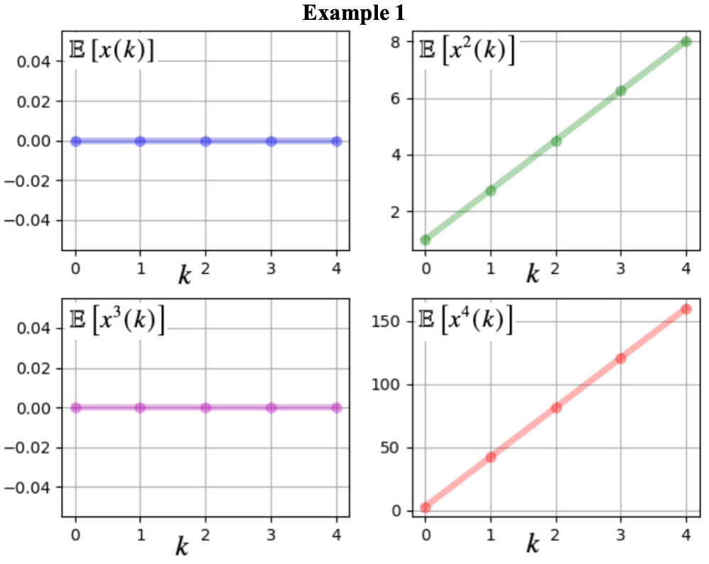
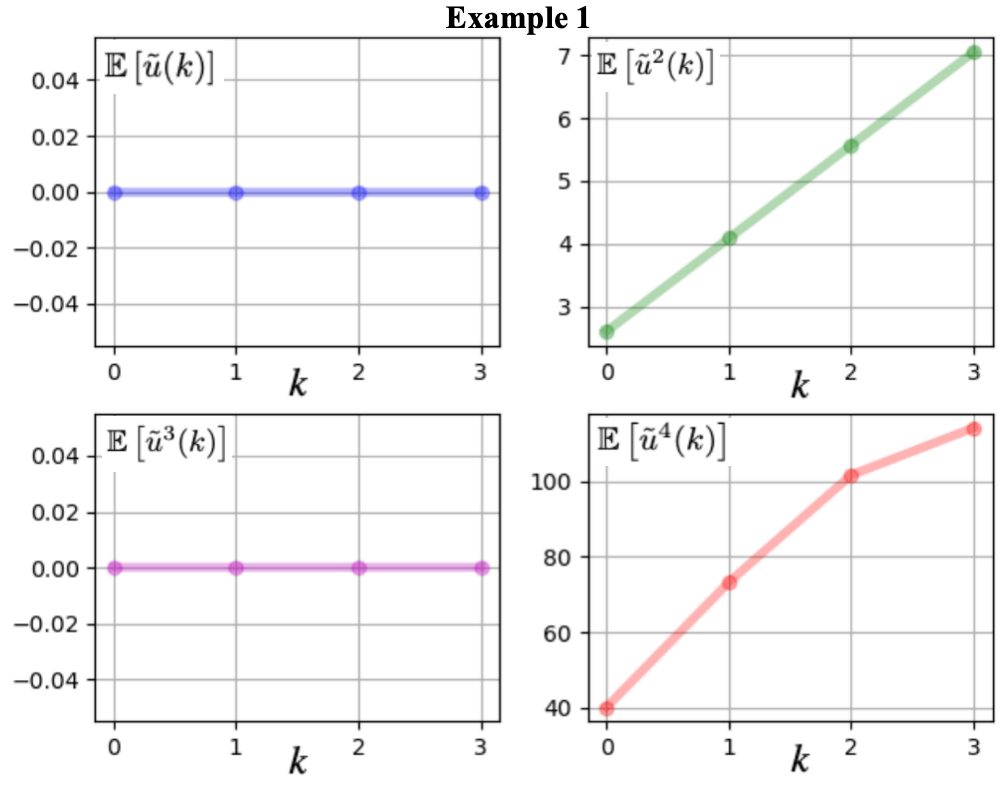
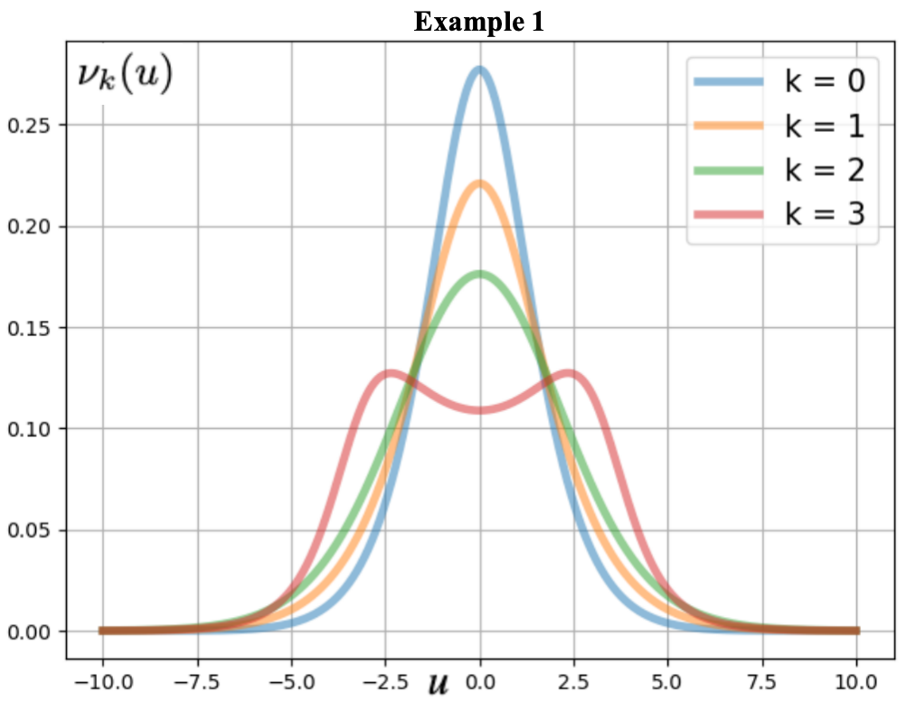
We note that even though the desired terminal distribution is a mixture of two Gaussian densities, it is unimodal. An example of a multi-modal distribution is given in Example 2. The system parameters $a(k),~{}k=0,1,\ldots,3$ are drawn from the uniform distribution $U([0.5,0.6])$. The system states of the moment system, i.e., $\mathscr{X}(k)$ for $k=0,1,2,3,4$ are given in Figure 1. The controls of the moment system, i.e., $\tilde{\mathscr{U}}(k)$ for $k=0,1,2,3$ are given in Figure 2. We note that $[\mathscr{X}(k)]_{H}\succ 0,[\tilde{\mathscr{U}}(k)]_{H}\succ 0$, which makes it feasible to realize the controls. The realized control inputs are given in Figure 3. The optimal values of $c(k)$ for this example are all zero.

Figure 1: $\mathscr{X}(k)$ at time steps $k=0,1,2,3,4$ for Example 1. The upper left figure shows $\mathbb{E}\left[x(k)\right]$. The upper right figure shows $\mathbb{E}\left[x^{2}(k)\right]$. The lower left figure shows $\mathbb{E}\left[x^{3}(k)\right]$ and the lower right figure shows $\mathbb{E}\left[x^{4}(k)\right]$.

Figure 2: Example 1: $\tilde{\mathscr{U}}(k)$ at time steps $k=0,1,2,3$. The upper left figure shows $\mathbb{E}\left[\tilde{u}(k)\right]$. The upper right figure shows $\mathbb{E}\left[\tilde{u}^{2}(k)\right]$. The lower left one shows $\mathbb{E}\left[\tilde{u}^{3}(k)\right]$ and the lower right figure shows $\mathbb{E}\left[\tilde{u}^{4}(k)\right]$.

Figure 3: Example 1: Realized distributions of control inputs $\nu_{k}(u)$ by $\tilde{\mathscr{U}}(k)$ for $k=0,1,2,3$, which are obtained by the proposed control scheme.

We use the obtained values of $\tilde{u}(k)~{}(k=0,1,\ldots,3)$ to steer $2,000$ agents to the specified distribution. The initial states of each agent $x_{i}$ are drawn i.i.d. from the Gaussian distribution (65). The system parameter for each agent $i$, namely $a_{i}(k)$ are i.i.d. samples drawn from the uniform distribution $U([0.5,0.6])$ for all $k=0,\ldots,3$.

Figure 4: The histograms of $u_{i}(k)$ at time step $k$ for each agent $i$. The upper row figures are $u_{i}(0)$ and $u_{i}(1),i=1,\ldots,2000$, respectively. The lower row figures are $u_{i}(2)$ and $u_{i}(3)$ ,respectively.

Figure 5: The histogram of the terminal distribution of $x_{i}(k),i=1,\ldots,2000$ compared to the desired distribution. It is close to the specified terminal distribution (66).

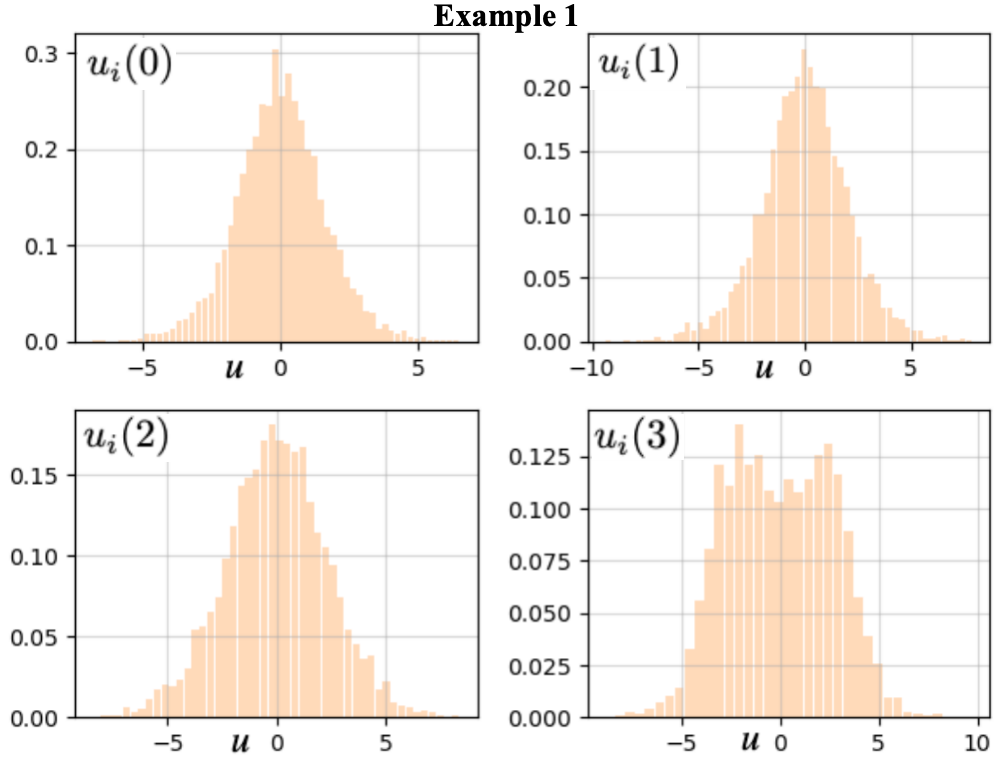
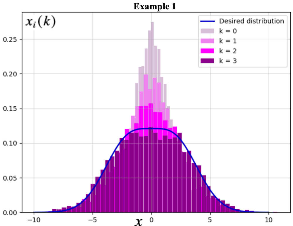
The histograms of $u_{i}(k)$ at time step $k$ for each agent $i$ are given in Figure 4. They are obtained using $2,000$ i.i.d samples drawn from the realizations of $\tilde{\mathscr{U}}(k)$ in Figure 3. Figure 5 shows the histogram of the terminal distribution of the states of the $2,000$ agents. We note that the final discrete distribution is close to the desired terminal distribution, thus validating our algorithm.

V-B Example 2: Linear ensemble system with system parameter following Laplace distribution

In the second example, we simulate a steering problem in four steps where the system parameter follows a Laplace distribution. The initial density is chosen as in (65). The terminal density function is specified as a multi-modal density which is a mixture of two Gaussian densities

$$\chi_{f}(x)=\frac{0.5}{\sqrt{2\pi}}e^{\frac{(x+2)^{2}}{2}}+\frac{0.5}{\sqrt{2\pi}}e^{\frac{(x-3)^{2}}{2}}.$$ (67)

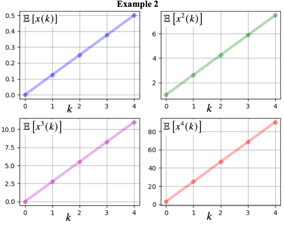
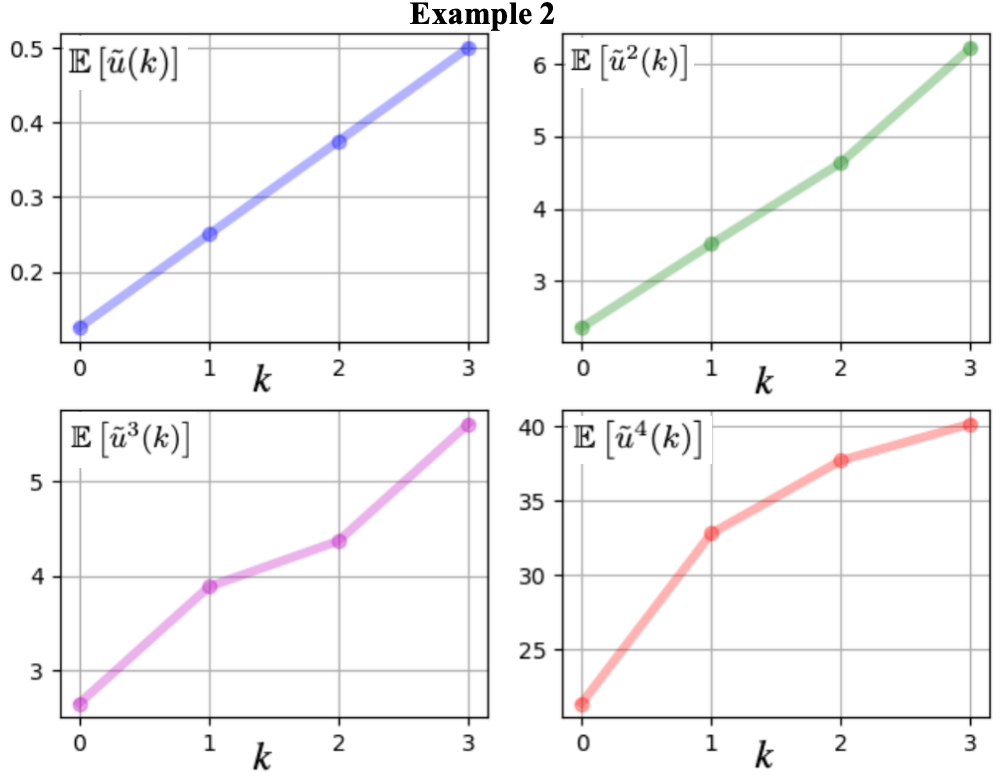
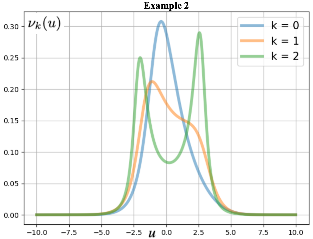
The system parameter $a(k)$ follows the Laplace distribution $\mathcal{C}\left(0.5,0.1\right)$ for all $k=0,1,2,3$. The results are given in Figures 6-10. The optimal values of $c(k)=0$ for $k=0,1,2$, and $c(3)=0.16$. In this example, the two peaks are not close to each other as in Example 1, which leads to two distinguishable modes. Since $c(3)\neq 0$, the corresponding $\tilde{\mathscr{U}}(3)$ is not positive definite, with its determinant being zero. This causes the control input $u(3)$ to be a discrete distribution supported on two points $-2.38,2.69$, with corresponding probability values $0.472,0.528$, respectively. From Figure 10, we note that the terminal discrete distribution using the proposed algorithm is close to the desired continuous one.

Figure 6: $\mathscr{X}(k)$ at time steps $k=0,1,2,3,4$.

Figure 7: $\tilde{\mathscr{U}}(k)$ at time steps $k=0,1,2,3$.

Figure 8: Realized distributions of control inputs $\nu_{k}(u)$ by $\tilde{\mathscr{U}}(k)$ for $k=0,1,2,3$, which are obtained by our proposed control scheme.

Figure 9: The histograms of $u_{i}(k)$ at time step $k$ for each agent $i$. The upper left and right figures are $u_{i}(0)$ and $u_{i}(1),i=1,\cdots,2000$ respectively. The lower left and right figures are $u_{i}(2)$ and $u_{i}(3)$ respectively.

Figure 10: The histogram of the terminal distribution of $x_{i}(k),i=1,\ldots,2000$ compared to the desired distribution. It is close to the specified terminal distribution (67).

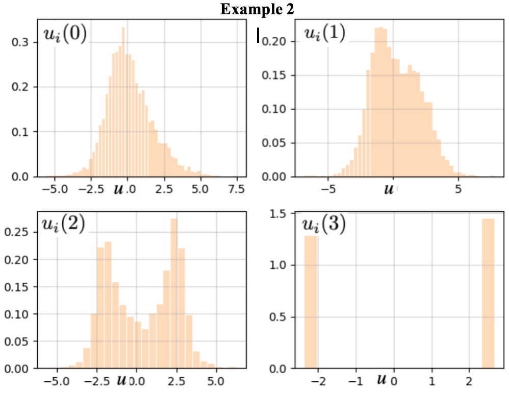
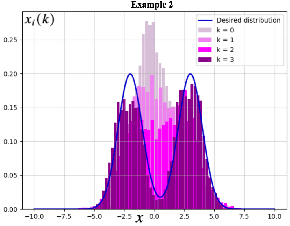
V-C Example 3: Linear ensemble system with multi-modal system parameter

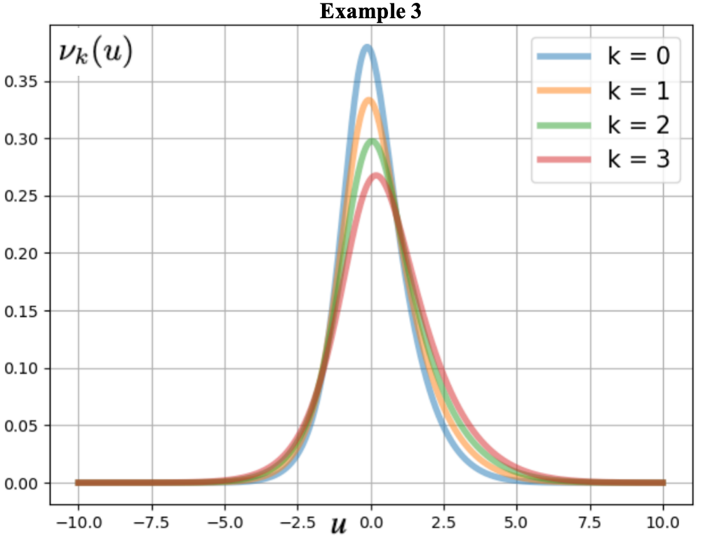
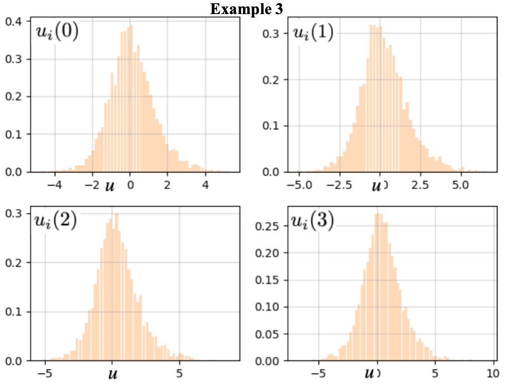
In this example, we consider the distribution steering problem where the system parameter $a_{i}(k)$ for each agent is from different modes, i.e., $a(k)$ is a multi-modal distribution. We consider $a(k)$ to be a mixture of Gaussian densities as follows

$$\alpha_{k}(a)=\frac{5}{2\sqrt{2\pi}}e^{\frac{25\,(a-0.3)^{2}}{2}}+\frac{5}{2\sqrt{2\pi}}e^{\frac{25\,(a-0.7)^{2}}{2}}.$$ (68)

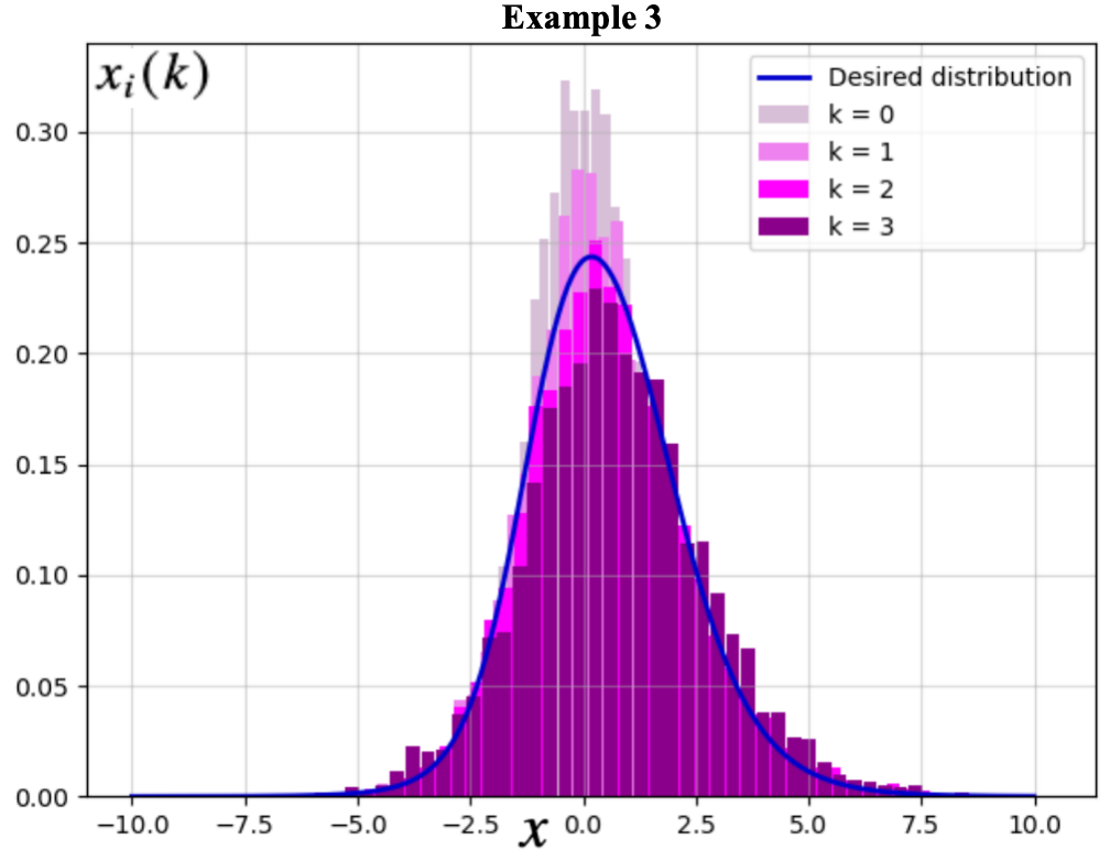
The initial density is again the unit Gaussian distribution as in (65) and the terminal density function is a multi-modal density, which is a mixture of two Type-I generalized Logistic densities

$$q_{f}(x)=\frac{0.5\,e^{-x+1}}{(1+e^{-x+1})^{2}}+\frac{0.5\,2e^{-x-1}}{(1+e^{-x-1})^{3}}.$$ (69)

The simulation results are given in Figure 11 to Figure 15. The optimal values of $c(k)$ are all zero. Figure 15 shows the terminal histogram of the states of $2,000$ agents which is close to the target distribution, as desired.

Figure 11: $\mathscr{X}(k)$ at time steps $k=0,1,2,3,4$.

Figure 12: $\tilde{\mathscr{U}}(k)$ at time steps $k=0,1,2,3$.

Figure 13: Realized distributions of control inputs $\nu_{k}(u)$ by $\tilde{\mathscr{U}}(k)$ for $k=0,1,2,3$, which are obtained by our proposed control scheme.

Figure 14: The histograms of $u_{i}(k)$ at time step $k$ for each agent $i$. The upper row figures are $u_{i}(0)$ and $u_{i}(1),i=1,\ldots,2000$, respectively. The lower row figures are $u_{i}(2)$ and $u_{i}(3)$, respectively.

Figure 15: The histogram of the terminal distribution of $x_{i}(k),i=1,\ldots,2000$ compared to the desired distribution. It is close to the specified terminal distribution (69).

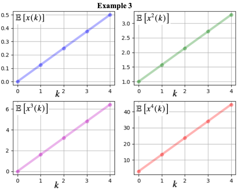
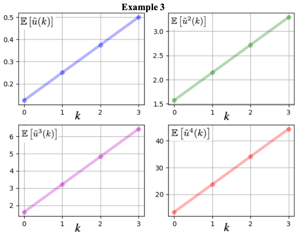
V-D Example 4: Nonlinear ensemble system with uniformly distributed system parameter

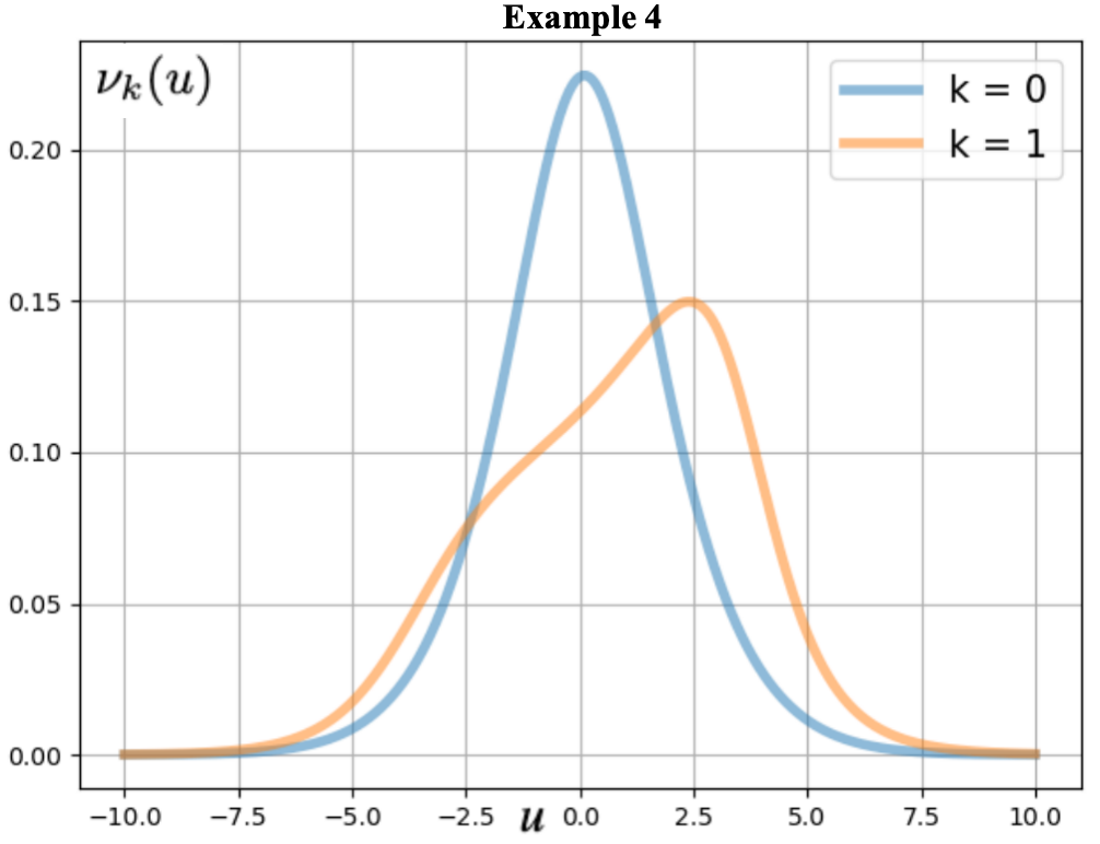
In this example, we consider a distribution steering problem in which the system dynamics is (51). We wish to steer the unit Gaussian density to a mixture of Gaussian densities in two steps $(K=2)$. The initial and the terminal distributions are the same as those in Example 1.

The results are given in Figures 11-15. The optimal values of $c(k)$ are all zero. In Figure 15, we observe that the terminal histogram of the states of $2,000$ agents approximates very well the desired distribution. This example validates the proposed algorithm for distribution steering with nonlinear system dynamics.

Figure 16: Realized distributions of control inputs $\nu_{k}(u)$ by $\tilde{\mathscr{U}}(k)$ for $k=0,1$, which are obtained by our proposed control scheme.

Figure 17: The histograms of $u_{i}(k)$ at time step $k$ for each agent $i$. The left and right figures are $u_{i}(0)$ and $u_{i}(1),i=1,\ldots,2,000$, respectively.

Figure 18: The histogram of the terminal distribution of the states of $2,000$ agents at time step $K=2$ compared to the desired distribution. It is close to the specified terminal distribution (69).

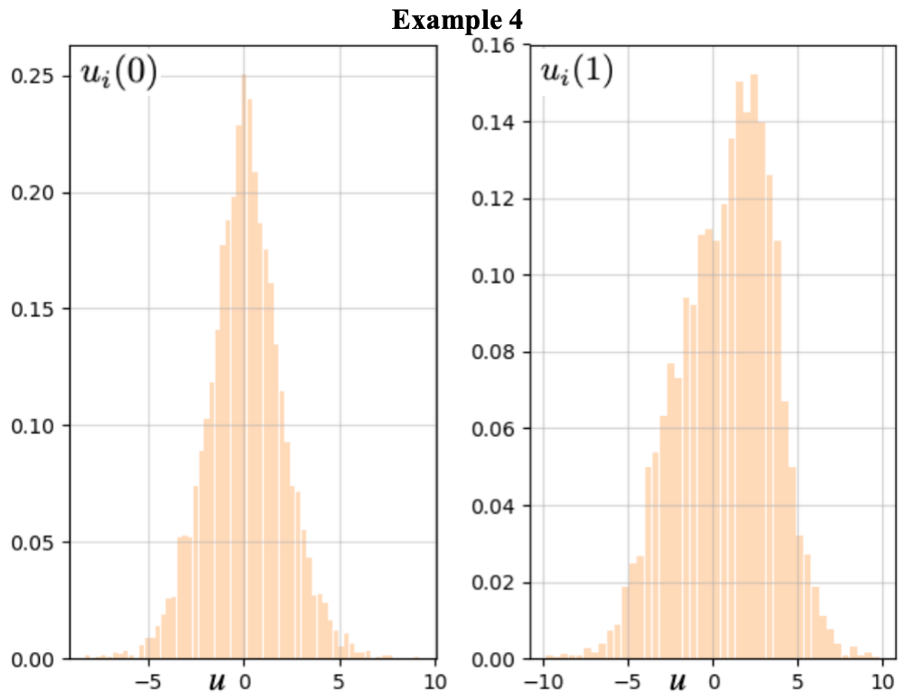
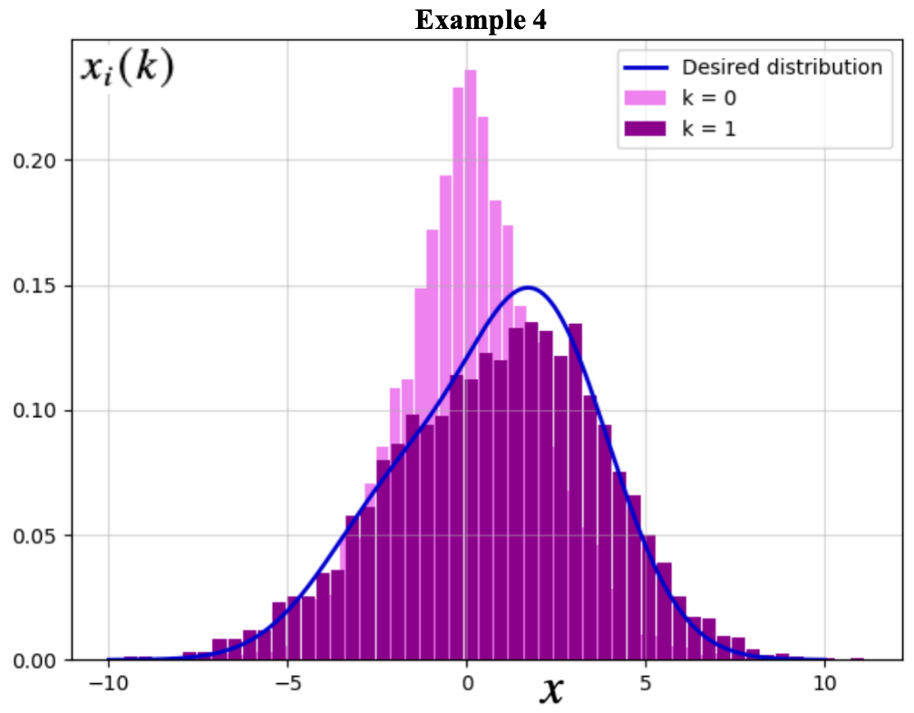
These four numerical examples demonstrate the effectiveness of the proposed scheme in addressing distribution steering problems for both linear and nonlinear first-order discrete-time ensemble systems. Moreover, the proposed solution scheme proves to be adaptable to various distributions of the system parameters. These numerical examples support the feasibility of the proposed algorithm as a viable solution for the general distribution steering problem.

VI Conclusions

Distribution steering is a fundamental challenge in stochastic control and swarm robotics. In conventional distribution steering problems, the uncertainty of the system state is represented by a probability distribution, typically assumed to be Gaussian. However, considering steering large groups of swarm robots, the distribution characterizes the entire group’s system state, making strict Gaussian assumptions inadequate [24, 25].

In this paper, we tackle the control of a large group of agents through a generalized distribution steering problem. We present a novel formulation for the dynamics of the ensemble system. Unlike traditional approaches, this distribution steering problem does not rely on assuming Gaussian distributions for the system states or the parameters. Instead, we require the existence of finite power moments up to order $2n$, where $n$ is some positive integer. To our knowledge, this algorithm is the first viable solution for the distribution steering of a large swarm robot group governed by general ODE systems with uncertainty in the system parameter.

Furthermore, the findings of this paper highlight the effectiveness of power moments in tackling infinite-dimensional stochastic control problems. By utilizing power moments, we represent both the uncertainty of the system parameter and the agents’ distribution as a whole. This leads to a significant simplification in propagating the system state during the control process. Power moments also serve as compact representations of the distribution’s macroscopic properties. As evidenced in the preceding numerical examples, the moment system of order $2n=4$ provides an accurate approximation of the original system, with our algorithm yielding a terminal distribution that closely matches the desired distribution.

Looking forward, future research will aim to extend the results of this paper to multiple-dimensional systems. However, such an extension poses major challenges. Ensuring the existence of the control inputs, namely, control inputs with non-negative probability density functions, poses a significant hurdle necessitating the application of tools from real algebraic geometry, e.g., Positivstellensätze.

Guangyu Wu (S’22) received the B.E. degree from Northwestern Polytechnical University, Xi’an, China, in 2013, and two M.S. degrees, one in control science and engineering from Shanghai Jiao Tong University, Shanghai, China, in 2016, and the other in electrical engineering from the University of Notre Dame, South Bend, USA, in 2018. He is currently pursuing the Ph.D. degree at Shanghai Jiao Tong University. His research interests include the moment problem and its applications to stochastic filtering, distribution steering, system identification and statistics. He is a reviewer of Automatica, IEEE Control Systems Letters, IEEE Conference on Decision and Control.

Panagiotis Tsiotras (F’19) received the Ph.D. degree in Aeronautics and Astronautics from Purdue University in 1993. He also holds degrees in Mechanical Engineering and Mathematics. He currently holds the David and Andrew Lewis Chair at the School of Aerospace Engineering at the Georgia Institute of Technology (Georgia Tech). He has held visiting research appointments at MIT, JPL, INRIA Rocquencourt, and Mines ParisTech. His research interests include optimal control of nonlinear systems and ground, aerial, and space vehicle autonomy. He has served on the Editorial Boards of the Transactions on Automatic Control, the IEEE Control Systems Magazine, the AIAA Journal of Guidance, Control and Dynamics, and the journal Dynamics and Control. He is the recipient of the NSF CAREER award, the Outstanding Aerospace Engineer award from Purdue, and the IEEE Award for Technical Excellence in Aerospace Control. He is a Fellow of AIAA and AAS.

Anders Lindquist (M’77–SM’86–F’89–LF’10) received the Ph.D. degree in Optimization and Systems Theory from the Royal Institute of Technology (KTH), Stockholm, Sweden, in 1972, an honorary doctorate (Doctor Scientiarum Honoris Causa) from Technion (Israel Institute of Technology) in 2010 and Doctor Jubilaris from KTH in 2022. He is currently a Distinguished Professor at Anhui University, Hefei, China, Professor Emeritus at Shanghai Jiao Tong University, China, and Professor Emeritus at the Royal Institute of Technology (KTH), Stockholm, Sweden. Before that he had a full academic career in the United States, after which he was appointed to the Chair of Optimization and Systems at KTH. Dr. Lindquist is a Member of the Royal Swedish Academy of Engineering Sciences, a Foreign Member of the Chinese Academy of Sciences, a Foreign Member of the Russian Academy of Natural Sciences (elected 1997), a Member of Academia Europaea (Academy of Europe), an Honorary Member the Hungarian Operations Research Society, a Life Fellow of IEEE, a Fellow of SIAM, and a Fellow of IFAC. He received the 2003 George S. Axelby Outstanding Paper Award, the 2009 Reid Prize in Mathematics from SIAM, and the 2020 IEEE Control Systems Award, the IEEE field award in Systems and Control.

References

- [1] E. Collins and R. Skelton, “Covariance control of discrete systems,” in Proc. IEEE Conf. Decision Control, (Lauderdale, FL), pp. 542–547, 1985.
- [2] E. Collins and R. Skelton, “A theory of state covariance assignment for discrete systems,” IEEE Transactions on Automatic Control, vol. 32, no. 1, pp. 35–41, 1987.
- [3] C. Hsieh and R. E. Skelton, “All covariance controllers for linear discrete-time systems,” IEEE Transactions on Automatic Control, vol. 35, no. 8, pp. 908–915, 1990.
- [4] J.-H. Xu and R. E. Skelton, “An improved covariance assignment theory for discrete systems,” IEEE Transactions on Automatic Control, vol. 37, no. 10, pp. 1588–1591, 1992.
- [5] K. Okamoto, M. Goldshtein, and P. Tsiotras, “Optimal covariance control for stochastic systems under chance constraints,” IEEE Control Systems Letters, vol. 2, no. 2, pp. 266–271, 2018.
- [6] K. Okamoto and P. Tsiotras, “Optimal stochastic vehicle path planning using covariance steering,” IEEE Robotics and Automation Letters, vol. 4, no. 3, pp. 2276–2281, 2019.
- [7] I. M. Balci and E. Bakolas, “Covariance steering of discrete-time stochastic linear systems based on Wasserstein distance terminal cost,” IEEE Control Systems Letters, vol. 5, no. 6, pp. 2000–2005, 2020.
- [8] F. Liu, G. Rapakoulias, and P. Tsiotras, “Optimal covariance steering for discrete-time linear stochastic systems,” arXiv preprint arXiv:2211.00618, 2022.
- [9] E. Bakolas, “Dynamic output feedback control of the Liouville equation for discrete-time SISO linear systems,” IEEE Transactions on Automatic Control, vol. 64, no. 10, pp. 4268–4275, 2019.
- [10] Y. Chen, T. T. Georgiou, and M. Pavon, “Optimal steering of a linear stochastic system to a final probability distribution, Part I,” IEEE Transactions on Automatic Control, vol. 61, no. 5, pp. 1158–1169, 2015.
- [11] Y. Chen, T. T. Georgiou, and M. Pavon, “Optimal steering of a linear stochastic system to a final probability distribution, Part II,” IEEE Transactions on Automatic Control, vol. 61, no. 5, pp. 1170–1180, 2015.
- [12] Y. Chen, T. T. Georgiou, and M. Pavon, “Optimal steering of a linear stochastic system to a final probability distribution, Part III,” IEEE Transactions on Automatic Control, vol. 63, no. 9, pp. 3112–3118, 2018.
- [13] M. Dorigo, G. Theraulaz, and V. Trianni, “Swarm robotics: Past, present, and future [point of view],” Proceedings of the IEEE, vol. 109, no. 7, pp. 1152–1165, 2021.
- [14] V. Strobel, A. Pacheco, and M. Dorigo, “Robot swarms neutralize harmful Byzantine robots using a blockchain-based token economy,” Science Robotics, vol. 8, no. 79, p. eabm4636, 2023.
- [15] S. Li, R. Batra, D. Brown, H.-D. Chang, N. Ranganathan, C. Hoberman, D. Rus, and H. Lipson, “Particle robotics based on statistical mechanics of loosely coupled components,” Nature, vol. 567, no. 7748, pp. 361–365, 2019.
- [16] M. Dorigo, G. Theraulaz, and V. Trianni, “Reflections on the future of swarm robotics,” Science Robotics, vol. 5, no. 49, p. eabe4385, 2020.
- [17] S. Zhang, A. Ringh, X. Hu, and J. Karlsson, “Modeling collective behaviors: A moment-based approach,” IEEE Transactions on Automatic Control, vol. 66, no. 1, pp. 33–48, 2020.
- [18] F. Bullo, J. Cortés, and S. Martinez, Distributed Control of Robotic Networks: A Mathematical Approach to Motion Coordination Algorithms, vol. 27. Princeton University Press, 2009.
- [19] M. Mesbahi and M. Egerstedt, “Graph theoretic methods in multiagent networks,” in Graph Theoretic Methods in Multiagent Networks, Princeton University Press, 2010.
- [20] V. Sivaramakrishnan, J. Pilipovsky, M. Oishi, and P. Tsiotras, “Distribution steering for discrete-time linear systems with general disturbances using characteristic functions,” in Proc. American Control Conference, (Atlanta, GA), pp. 4183–4190, 2022.
- [21] A. Ringh, I. Haasler, Y. Chen, and J. Karlsson, “Mean field type control with species dependent dynamics via structured tensor optimization,” IEEE Control Systems Letters, 2023.
- [22] V. Deshmukh, K. Elamvazhuthi, S. Biswal, Z. Kakish, and S. Berman, “Mean-field stabilization of Markov chain models for robotic swarms: Computational approaches and experimental results,” IEEE Robotics and Automation Letters, vol. 3, no. 3, pp. 1985–1992, 2018.
- [23] K. Elamvazhuthi, S. Biswal, and S. Berman, “Mean-field stabilization of robotic swarms to probability distributions with disconnected supports,” in Proc. American Control Conference, (Milwaukee, WI), pp. 885–892, 2018.
- [24] S. Biswal, K. Elamvazhuthi, and S. Berman, “Stabilization of nonlinear discrete-time systems to target measures using stochastic feedback laws,” IEEE Transactions on Automatic Control, vol. 66, no. 5, pp. 1957–1972, 2020.
- [25] S. Biswal, K. Elamvazhuthi, and S. Berman, “Decentralized control of multiagent systems using local density feedback,” IEEE Transactions on Automatic Control, vol. 67, no. 8, pp. 3920–3932, 2021.
- [26] I. Nodozi, J. O’Leary, A. Mesbah, and A. Halder, “A physics-informed deep learning approach for minimum effort stochastic control of colloidal self-assembly,” in Proc. American Control Conference, (San Diego, CA), pp. 609–615, 2023.
- [27] K. F. Caluya and A. Halder, “Wasserstein proximal algorithms for the Schrödinger bridge problem: Density control with nonlinear drift,” IEEE Transactions on Automatic Control, vol. 67, no. 3, pp. 1163–1178, 2021.
- [28] K. F. Caluya and A. Halder, “Gradient flow algorithms for density propagation in stochastic systems,” IEEE Transactions on Automatic Control, vol. 65, no. 10, pp. 3991–4004, 2019.
- [29] K. Elamvazhuthi, P. Grover, and S. Berman, “Optimal transport over deterministic discrete-time nonlinear systems using stochastic feedback laws,” IEEE control systems letters, vol. 3, no. 1, pp. 168–173, 2018.
- [30] J.-S. Li and N. Khaneja, “Ensemble control of Bloch equations,” IEEE Transactions on Automatic Control, vol. 54, no. 3, pp. 528–536, 2009.
- [31] J.-S. Li, “Ensemble control of finite-dimensional time-varying linear systems,” IEEE Transactions on Automatic Control, vol. 56, no. 2, pp. 345–357, 2010.
- [32] G. Wu and A. Lindquist, “Density steering by power moments,” in Proc. IFAC World Congress, (Yokohama, Japan), pp. 3423–3428, 2023.
- [33] G. Wu and A. Lindquist, “General distribution steering: A sub-optimal solution by convex optimization,” arXiv preprint arXiv:2301.06227, 2023.
- [34] K. Elamvazhuthi and S. Berman, “Mean-field models in swarm robotics: A survey,” Bioinspiration & Biomimetics, vol. 15, no. 1, p. 015001, 2019.
- [35] G. Wu and A. Lindquist, “Group steering: Approaches based on power moments,” arXiv preprint arXiv:2211.13370, 2022.
- [36] J. Ridderhof, K. Okamoto, and P. Tsiotras, “Nonlinear uncertainty control with iterative covariance steering,” in Proc. IEEE Conference on Decision and Control, (Nice, France), pp. 3484–3490, 2019.
- [37] L. Tie and J.-S. Li, “On controllability of discrete-time linear ensemble systems with linear parameter variation,” in Proc. American Control Conference, (Boston, MA), pp. 6357–6362, 2016.
- [38] N. Mandal, M. Khajenejad, and S. Martinez, “Control of Discrete-Time LTI Systems using Stochastic Ensemble Systems,” arXiv preprint arXiv:2304.11755, 2023.
- [39] P. Stavroulakis, Distributed Parameter Systems Theory: Estimation. Hutchinson Ross, 1983.
- [40] A. Feintuch, Robust Control Theory in Hilbert Space, vol. 130. Springer Science & Business Media, 2012.
- [41] J. Pitman, “Occupation measures for Markov chains,” Advances in Applied Probability, vol. 9, no. 1, pp. 69–86, 1977.
- [42] K. Schmüdgen, The Moment Problem, vol. 277. Graduate Texts in Mathematics, Springer, 2017.
- [43] O. Glass, “Infinite dimensional controllability,” Encyclopedia of Complexity and Systems Science, p. 4804–4820, 2009.
- [44] S. Boyd and L. Vandenberghe, Convex Optimization. Cambridge University Press, 2004.
- [45] C. I. Byrnes, S. V. Gusev, and A. Lindquist, “From finite covariance windows to modeling filters: A convex optimization approach,” SIAM Review, vol. 43, no. 4, pp. 645–675, 2001.
- [46] C. I. Byrnes, P. Enqvist, and A. Lindquist, “Identifiability of shaping filters from covariance lags, cepstral windows and Markov parameters,” in Proceedings of the 41st IEEE Conference on Decision and Control, 2002., vol. 1, pp. 246–251, IEEE, 2002.
- [47] T. T. Georgiou and A. Lindquist, “Kullback-Leibler approximation of spectral density functions,” IEEE Transactions on Information Theory, vol. 49, no. 11, pp. 2910–2917, 2003.
- [48] G. Wu and A. Lindquist, “Non-Gaussian Bayesian filtering by density parametrization using power moments,” Automatica, vol. 153, p. 111061, 2023.
- [49] L. Mátyás, Generalized Method of Moments Estimation, vol. 5. Cambridge University Press, 1999.
- [50] W. Rudin, Real and Complex Analysis. McGraw Hill Education India, 2015.
![[Uncaptioned image]](/html/2405.12415/assets/author1.jpg) |