Remaining Energy Prediction for Lithium-Ion Batteries: A Machine Learning Approach
Abstract
Lithium-ion batteries have found their way into myriad sectors of industry to drive electrification, decarbonization, and sustainability. A crucial aspect in ensuring their safe and optimal performance is monitoring their energy state. In this paper, we present the first study on predicting the remaining energy of a battery cell undergoing discharge over wide current ranges from low to high C-rates. The complexity of the challenge arises from the cell’s C-rate-dependent energy availability as well as its intricate electro-thermal dynamics. To address this, we introduce a new definition of remaining discharge energy and then undertake a systematic effort in harnessing the power of machine learning to enable its prediction. Our effort includes two parts in cascade. First, we develop an accurate dynamic model based on integration of physics with machine learning to capture a battery’s voltage and temperature behaviors. Second, based on the model, we propose a machine learning approach to predict the remaining discharge energy under arbitrary C-rates and pre-specified cut-off limits in voltage and temperature. The results from our experiments show that the proposed approach offers high prediction accuracy and amenability to training and computation.
keywords:
Lithium-ion batteries , machine learning , neural networks , remaining discharge energy[inst1]organization=Department of Mechanical Engineering, University of Kansas,city=Lawrence, postcode=KS 66045, country=USA
[inst4]organization=Department of Electrical Engineering, Tezpur University,city=Tezpur, postcode=784028, country=India
[inst2]organization=Department of Civil and Environmental Engineering, University of California,city=Berkeley, postcode=CA 94720, country=USA
[inst3]organization=Mitsubishi Electric Research Laboratories,city=Cambridge, postcode=MA 02139, country=USA
1 Introduction
Lithium-ion batteries (LiBs) represent one of the most important power source technologies of our time. They have transformed the consumer electronics sector since the 1990s and are now driving the revolution of transportation electrification that extends from passenger cars to commercial vehicles to aircraft. Battery management systems (BMSs) must be in place for the use of LiBs to ensure their safety and performance. Among the various BMS functions, a significant one is monitoring the state of energy or, more specifically, the remaining discharge energy (RDE). While its definition may take different forms, the RDE, in general, indicates how much energy is available before the cell gets depleted in discharging. Practical applications demand accurate, real-time RDE prediction to avoid over-discharging or determine the remaining duration or range in power supply. However, the prediction is non-trivial due to the complex dynamics of LiBs, which has attracted a growing body of research in recent years.
A quantity closely related to the RDE is the so-called state-of-charge (SoC), which is the percentage ratio between a cell’s available charge capacity in Ah and its nominal capacity. While the estimation of it has received extensive study in the literature [1, 2, 3, 4, 5, 6, 7], the SoC does not align with the cell’s actual level of energy in Wh [8]. As a case in point, the amount of energy the cell can deliver in the low SoC range is less than that in the high SoC range. By definition, the SoC also factors out the rate-capacity effect, which refers to the phenomenon of the deliverable charge or energy capacity becoming less (resp. more) under higher (resp. lower) discharging C-rates [9].
Compared to the SoC, the RDE comes as a more direct measure of the cell’s remaining energy. RDE prediction has attracted growing interest, and the studies to date fall into two categories. In the first category, the RDE is defined as the percentage ratio of the cell’s present energy over the maximum energy [8]. Based on the definition, different models can be constructed to relate the RDE with the cell’s current, voltage, and temperature. Given the models supplemented with measurement data, one can apply various nonlinear state estimation methods, such as Kalman filtering, particle filtering and their variants, to identify the RDE [10, 11, 12, 13, 14, 15, 16]. Studies of the second category take the approach of model-based forward simulation. They propose to solve the model forward until some cut-off limits are reached and then calculate the total energy released in each run [17, 18, 19, 20].
Despite the many promising developments in RDE prediction, the state of the art is still limited. Existing works generally consider discharging at low to medium currents. In this case, the RDE is almost linear with the SoC [9], so the estimation of RDE bears little difference from SoC estimation. However, more interesting and useful is RDE prediction for discharging that spans low to high currents. The problem conveys more challenges while proving crucial for some emerging applications like electric aircraft [21], but the literature is void of studies to deal with it. We also note that some RDE prediction methods, e.g., those based on model-based forward simulation, require heavy computation. Practical applications, however, demand methods that are computationally efficient and amenable to implementation.
Motivated to overcome the above limitations, this paper, for the first time, explores the intricate task of RDE prediction over broad C-rate ranges and develops a solution framework based on machine learning (ML). The contribution is twofold.
-
1.
We propose a new RDE definition suitable for the considered problem. Different from its counterparts in the literature, the definition makes RDE dependent on C-rates and takes into account both the voltage limit and temperature limit.
-
2.
Following the definition, we develop a novel ML approach to achieve accurate RDE prediction. This approach is designed to capture mappings from the cell’s operating state to the remaining energy at a future time, while addressing some tricky issues in determining the remaining discharge time. To train the ML approach, we develop a separate hybrid physics+ML model to generate high-fidelity synthetic training data. The hybrid model is an extension of our prior work in [22], which can accurately captures a LiB cell’s voltage and thermal dynamics over broad current ranges.
The proposed RDE prediction approach is accurate, tractable for training, and computationally fast. We validate its effectiveness through extensive experiments on a nickel-cobalt-aluminum (NCA) cell and a lithium-iron-phosphate (LFP) cell.
The remainder of the paper is organized as follows. Section 2 proposes the definition of the C-rate-dependent RDE. Section 3 presents the hybrid physics-ML model to predict a LiB cell’s voltage and temperature in discharging over broad current ranges. Section 4 presents an ML-based RDE prediction approach. Then, the experimental validation results are shown in Section 5. Finally, Section 6 concludes the paper.
2 Definition of C-rate-dependent RDE
This section proposes a new definition of RDE for LiBs. Different from other versions, this definition is designed to capture the variation of a cell’s remaining available energy over different C-rates. Accurate and real-time prediction of the proposed RDE will be the aim of the subsequent sections.
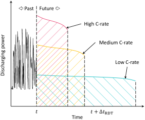
In general, the energy that a LiB cell will release over an upcoming time interval is the integration of its discharging power. This quantity, however, is neither constant nor fixed. Indeed, it is dependent on the discharging C-rate as a result of two main factors. First, the cell’s output voltage will decline faster when the discharging current increases, leading to less energy being released. This phenomenon is known as the rate-capacity effect. Second, the C-rate will greatly influence the cell’s temperature. The discharging process and, consequently, the amount of energy that is to be discharged will be subject to the upper temperature limit for safety. Therefore, it is important and necessary to take the C-rate into account when defining the RDE when the cell operates over broad current ranges. We consider the RDE as the amount of the remaining energy if the cell is discharged at a constant C-rate from the present time until when either the voltage or the temperature limit is reached. With this notion, the RDE is defined as follows:
| (1) |
where is the present time, is the remaining discharging time, is the future discharge C-rate between and , is the current of 1 C-rate in ampere, is the cell’s voltage. Note that is the time when the cell reaches the cut-off voltage or the maximum allowed temperature if discharged at the constant current of C-rate. Fig. 1 illustrates this proposed RDE definition.
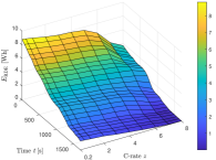
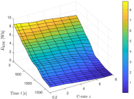
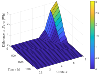
The RDE definition in (1) is a departure away from alternative definitions in the literature which overlook the effects of the C-rates [9]. The validity and necessity of proposing it is shown in Fig. 2. Here, Fig. 2a illustrates of an NCA cell under different C-rates subject to and , highlighting the substantial variation of with the C-rate. Additionally, Fig. 2b shows the scenario when is disregarded. Upon comparison with Fig. 2a, a significant difference emerges at high C-rates, as depicted in Fig. 2c. This observation underscores the considerable influence of high C-rates on the cell’s thermal behavior, while emphasizing the importance of considering .
Given the proposed definition, next we compute and predict the RDE for a LiB cell. However, this involves multiple challenges. First, we need a model that is capable of accurately predicting the cell’s voltage and temperature over broad current ranges. Second, even after the model is available, can still be hard to determine as it depends on a mix of the cell’s present state, future behavior at designated , and pre-specified and limits. Finally, online prediction of the RDE is desired, but how to achieve real-time computational efficiency is a question. In the sequel, we will develop a methodical approach to tackle these challenges by utilizing the capabilities of ML. An overview of our study is shown in Fig. 4.
3 Hybrid Physics-ML Modeling for LiBs

This section aims to develop a dynamic model to predict the terminal voltage and temperature of a LiB cell with fast computation and high accuracy when the cell discharging spans broad C-rate ranges. Toward this end, we take the approach of integrating physics with ML. For physics-based modeling, we use the nonlinear double capacitor (NDC) model [23] for voltage prediction and a lumped thermal circuit model [24] for temperature prediction. The NDC model is an equivalent circuit model, which is computationally fast and accurate over low to medium C-rates. Nonetheless, it lacks predictive capability at high C-rates. The same occurs to the lumped thermal circuit model. We, therefore, put these two physics-based models in cascade with two separate feedforward neural networks (FNNs) so that the FNNs can use the physics to make predictions.
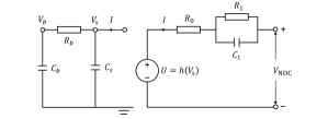
We begin by introducing the NDC model and the lumped thermal model. The NDC model describes a LiB cell’s electric behavior and, different from other equivalent circuit models, includes a mechanism to emulate the impact of lithium-ion diffusion on the voltage dynamics. As shown in Fig. 3a, the model contains two coupled sub-circuits. The first (left) sub-circuit contains an R-C chain composed of , and . Conceptually, and represent the bulk inner region and surface region of the electrode, respectively, and the migration of charge between and mimics the lithium-ion diffusion within the electrode. The second (right) sub-circuit contains a voltage source , a resistor , and an R-C pair -. Here, serves as an open-circuit voltage source, corresponds to the ohmic resistance and solid electrolyte interface resistance, and - accounts for the voltage transients due to charge transfer on the electrode/electrolyte interface. The governing equations of the NDC model are given by
| (2a) | ||||
| (2b) | ||||
where , and are the voltages across , and , respectively, and is the input current ( for discharge, for charge). Here,
The lumped thermal model, as shown in Fig. 3b, assumes a cylindrical shape of the cell and concentrates the spatially distributed temperature radially into two points at the cell’s core and the surface, respectively. The model then is governed by
| (3) |
where
is the temperature at the core/surface of the cell, is the ambient temperature, and is the heat capacity at the cell’s core/surface. Further, is the thermal resistance due to the conduction between the core and surface, and is the thermal resistance due to the convection between the cell’s surface and the environment. This model only considers internal heat generation at the core that results from Joule heating.
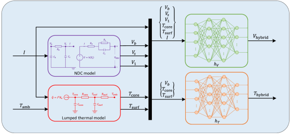
The above two ECMs have decent accuracy at low to medium currents but lack accuracy for high currents. To overcome the gap, we couple them with ML models. ML has strong data-driven representation capabilities, and we have shown in our prior studies [22] that they can predict the behaviors of a LiB cell with high accuracy if integrated with physics-based models. Based on the insights in [22], we propose the NDCTNet model in Fig. 4a, which characteristically connects the above two ECMs with two separate FNNs in series. The first FNN is responsible for the terminal voltage prediction. It takes , , , , and as the inputs. The second FNN is meant to predict the surface temperature, and its input includes , and . Here, the FNNs are made to use physical state information for prediction. This allows to use simpler FNNs, reduce data dependence in training, and achieve more accurate prediction. It should be noted that the inputs to the FNNs must be selected so that the FNNs can capture physically justifiable and sound mappings (an interested reader is referred to [22] for more discussion). The proposed choice is the best one that we could find after many trials, though there may exist alternatives.
In summary, the NDCTNet model can be written in the following mathematical form:
| (4a) | ||||
| (4b) | ||||
| (4c) | ||||
where , (4a) results from (2a) and (3) and is a linear ordinary differential equation, and and represent the two FNNs.
To identify the NDCTNet model, we first extract the NDC model and the thermal circuit model from datasets which include the cell’s current, voltage and surface temperature collected at discharging at low to medium C-rates [23]. Then, we collect the cell’s current, voltage and surface temperature at high C-rates, together with the states of both the NDC and the thermal circuit model, and use them to train the FNNs by minimizing the difference between (resp. ) and the actual terminal voltage (resp. actual surface temperature). The reader is referred to [22] for more information.
4 Real-Time RDE Prediction via NNs
In this section, we focus on the problem of real-time RDE prediction for LiBs. Note that, given the LiB model developed in Section 3, a straightforward approach to the RDE prediction is to forward run the NDCTNet model from the present state until or is reached, as is reported in some existing studies, e.g., [20]. However, this approach requires high computational costs. This is because not only the model execution may take a long time, as the actual discharging can be up to hours, but also the model must be solved for different C-rates from low to high. Therefore, we propose an ML-based approach to enable real-time RDE prediction. This new approach will eliminate the need for repetitive forward model simulation as ML models can give predictions efficiently after being trained. Also, we can harness the capacity of ML to achieve high RDE prediction accuracy given abundant data.
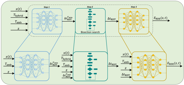
Based on the definition of in (1), we aim to train an FNN which will output based on the present state , and . Here, a key problem is to determine . As the remaining discharging time, will depend on whichever of and comes first in discharging. That is
| (5) |
where (resp. ) is the time duration that elapses before the cell reaches (resp. ). It should be noted that both and are -dependent. We find out that there exists a mapping from , and to , which can be captured by an FNN. However, is much more difficult to compute. The cell constantly has heat exchange with the ambient environment, and the ambient temperature, , can be arbitrary. This makes it intractable to train an FNN to predict . Instead, we use the bisection method to find if the cell will indeed exceed before the elapse of . To sum up the above, the proposed RDE prediction approach includes the following three steps:
-
1.
leverage an FNN to compute based on , and ;
-
2.
let = if ; otherwise, use the bisection search to find out , and let = ;
-
3.
given , use an FNN to predict based on , and .
Below we present the details of the three-step RDE prediction approach.
4.1 Computation of
The first step of our RDE prediction approach is to use an FNN to predict based on the triplet (, , ). However, one may wonder whether FNNs are able to perform the task. It is known that FNNs are suitable for approximating continuous mappings due to the universal approximation theorem [25], so the question is whether there exists such a mapping from (, , ) to a unique . To find the answer, we conduct the following analysis.
We begin with considering (4). Note that (4a) is a linear time-invariant system and thus has a closed-form solution. Letting be the initial condition, we express the solution for an arbitrary time interval under given and as
The exact formula for is available analytically. Then,
| (6) |
where denotes the operation of function composition. We further define and absorb into it for notational simplicity. Thus, satisfies
| (7) |
The following observations arise out of the equality in (7). First, by selecting a suitable activation function for the NNs, is continuously differentiable because both and are continuously differentiable. Second, for any physically possible (, , ), there always exists a unique in discharging to make (7) hold true. Third, from a physical perspective, it is arguable that an open neighborhood of (, , ) would correspond to an open neighborhood of . Finally, when the cell is continuously discharged starting from and under given and , its terminal voltage will decline monotonically when the discharging time approaches . This implies
Then, by the global implicit function theorem in [26], there is a unique and continuous mapping from (, , ) to . With the existence of such a mapping, an FNN can be used to predict based on (, , ).
4.2 Computation of
In predicting the RDE, we must take the cell’s future temperature into account to ensure that the prediction lies within the thermal safety bounds. This is particularly vital when the cell runs at high C-rates or under high ambient temperature. We have defined earlier to capture the effect of on the discharging time. Note that needs to be computed for the RDE prediction only when it is less than , as implied by (5). Therefore, it is plausible to expediently determine whether , and in case of not, a fast search for will ensue next.
To check , we pick checkpoints, for , which spread evenly within the interval . One may choose an appropriate , depending on the characteristics of the cell’s thermal dynamics and the immediate ambient conditions. Then, is computed for each via
The computation would be efficient, thanks to the explicit formula of . We can skip the calculation of if for all . Otherwise, we must determine , and this is equivalent to finding the root of
| (8) |
for which is the unknown variable. To this end, we apply the bisection method, a popular and efficient root-finding algorithm.
The bisection search is conducted within the interval . Initially, with , and . Assume that there is only one root for (8) within the initial interval. Subsequently, we bisect the interval, evaluate at the midpoint, identify the next subinterval to search, and repeat the search procedure. The steps are as follows.
-
[Step 1]
calculate , and evaluate ;
-
[Step 2]
let and stop if ; otherwise, go to Step 3.
-
[Step 3]
let if , and let if otherwise; go to Step 1.
Fig. 5 shows a flowchart of the procedure. The bisection search can find out fast here. This is because an explicit formula is available for the computation of , and the bisection method converges fast by itself when a unique root exists within the search interval.
4.3 Prediction of
After identifying , we are now ready to enable the prediction of . It is beneficial here to consider a more general task — predicting , which is the discharging energy released by the cell within the upcoming time interval under a constant C-rate :
When it is available, we can easily compute as
| (9) |
Given (6), we have
| (10) |
This relation indicates that there exists a continuous mapping from (, , , ) to . While there is no analytic form of the mapping, we can use an FNN to approximate it. The FNN is denoted as
After the FNN is trained, we can compute by (9).
Fig. 4b presents the pipeline of the proposed RDE prediction approach. To sum up, it is challenging to predict the RDE when the cell shows complex voltage and thermal behaviors under discharging across low to high currents. To overcome the problem, we turn our attention to utilizing the power of ML. We exploit FNNs to capture the sophisticated relationship between the RDE and the many factors that affect it. The approach presents several benefits. First, it is amenable to training. This is because we can train the FNNs on synthetic data generated by running the NDCTNet model in Section 3. This greatly reduces reliance on data collection from experiments. Second, the approach can attain high accuracy when the NDCTNet model is accurate enough to generate good-quality training data in large amounts. Finally, the prediction is computationally fast and efficient after the training.
We highlight that the proposed approach differs from existing RDE prediction methods in multiple ways. As the primary difference, the study is the first to consider the problem of RDE prediction under discharging over broad current ranges. It is also the first to incorporate the temperature limit into the prediction, contrasting with the negligence of this important factor in the literature. Our approach design is based on the notion of ML and justified in rationale, which has not been done in previous studies on RDE prediction.
5 Experimental Validation
| NCA | LFP | |
| Nominal capacity (Ah) | 2.5 | 2.5 |
| Allowed voltage range (V) | 2.54.2 | 2.03.6 |
| Max. continuous discharge current (A) | 20 | 50 |
| Operating surface temperature () | -2075 | -3055 |
| LiB type | Current profile | RMSE | RMSE |
| NCA | US06 (08 C) | 12.25 mV | 0.27 |
| SC04 (08 C) | 13.36 mV | 0.56 | |
| LFP | US06 (015 C) | 13.01 mV | 0.28 |
| SC04 (015 C) | 11.11 mV | 0.46 |
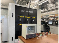
In this study, the experimental validation is performed on two cylindrical LiB cells: a Samsung INR18650-25R cell with an NCA cathode and graphite anode, and an A123 ANR26650-M1B cell with an LFP cathode and a graphite anode. Table 1 lists their specifications. A PEC® SBT4050 battery tester shown in Fig. 6 was used to charge/discharge the cells and collect experimental data. A host computer with a 2.2 GHz Intel® i7-8750H CPU and 16.0 GB RAM was used to process data and calculate RDE. A thermocouple was attached to each cell’s surface to measure its temperature. During the experiments, the cells were placed in a thermal chamber with the ambient temperature set to .
The validation consists of two stages. In the first stage, we identify and validate the NDCTNet model constructed in Section 3. In the second stage, we run the hybrid model in simulations to generate the data and train the RDE prediction approach. After the training, we implement the approach and compare its RDE prediction results with experimental data.
5.1 Training and Validation of the NDCTNet Model
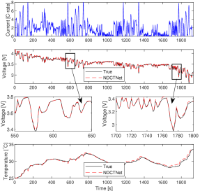
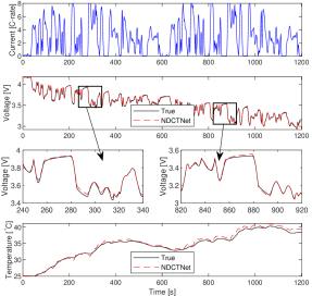
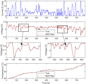
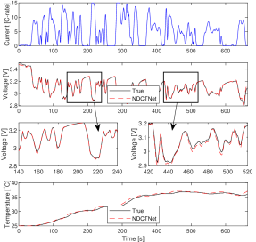
We used the following procedure to construct and validate the NDCTNet model for each of the two cells.
As the first step, we identified the NDC model and the lumped thermal model for each cell based on the methods in [23, 24]. Then, we moved on to train the FNNs of each NDCTNet model.
-
1.
We used the same FNN architecture for and for both cells. The FNN has two hidden layers with 48 neurons in each hidden layer. The softplus function is used as the activation function of the hidden layers, and the output layer employs the linear activation function.
-
2.
For the NCA cell, we collected the training datasets via constant-current discharging at 0.5/1/3/5/8 C and variable-current discharging based on the HWFET/UDDS/WLTC/LA92 profiles (scaled to 08 C) [27].
-
3.
For the LFP cell, the training datasets were generated by constant-current discharging at 0.5/1/2/4/6/8/10/12/15 C and variable-current discharging based on the HWFET/UDDS/WLTC/LA92 profiles (scaled to 015 C).
Further, we collected extra datasets based on the US06/SC04 profiles, scaled to 08 C for the NCA cell and 015 C for the LFP cell, to test the NDCTNet model after training. Figs. 7-8 present the validation results, which show excellent fitting performance. Table 2 offers a quantitative evaluation, indicating that the NDCTNet model exhibits high accuracy over broad current ranges for each cell.
5.2 Validation of the RDE Prediction Approach
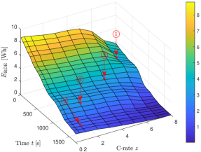
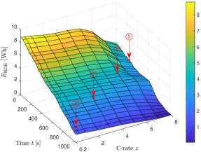
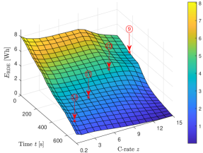
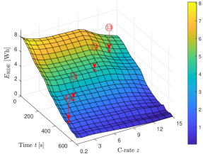
| LiB type | Current profile | Time instant (s) | C-rate | True (s) | Predicted (s) | prediction error (%) | True (Wh) | Traditional (Wh) | Predicted (Wh) | prediction error (%) | |
| \scalebox{0.65}1⃝ | NCA | US06 (08 C) | 389 | 7 | 221 | 231 | 4.52 | 3.64 | 6.42 | 3.56 | 2.20 |
| \scalebox{0.65}2⃝ | 775 | 5 | 279 | 279 | 0 | 3.14 | 4.39 | 3.11 | 0.96 | ||
| \scalebox{0.65}3⃝ | 1161 | 2 | 569 | 574 | 0.88 | 2.66 | 3.30 | 2.62 | 1.50 | ||
| \scalebox{0.65}4⃝ | 1547 | 1 | 601 | 639 | 6.32 | 1.47 | 1.95 | 1.43 | 2.72 | ||
| \scalebox{0.65}5⃝ | SC04 (08 C) | 243 | 8 | 148 | 154 | 4.05 | 2.81 | 7.09 | 2.73 | 2.85 | |
| \scalebox{0.65}6⃝ | 483 | 6 | 267 | 276 | 3.37 | 3.69 | 5.18 | 3.58 | 2.98 | ||
| \scalebox{0.65}7⃝ | 723 | 3 | 435 | 445 | 2.30 | 3.09 | 3.90 | 2.99 | 3.24 | ||
| \scalebox{0.65}8⃝ | 963 | 0.5 | 1343 | 1396 | 3.95 | 1.63 | 2.02 | 1.58 | 3.07 | ||
| \scalebox{0.65}9⃝ | LFP | US06 (015 C) | 159 | 15 | 126 | 120 | 4.76 | 3.50 | 6.58 | 3.59 | 2.57 |
| \scalebox{0.65}{10}⃝ | 315 | 10 | 192 | 195 | 1.56 | 3.87 | 5.16 | 3.84 | 0.78 | ||
| \scalebox{0.65}{11}⃝ | 471 | 5 | 269 | 263 | 2.23 | 2.72 | 3.63 | 2.79 | 2.57 | ||
| \scalebox{0.65}{12}⃝ | 627 | 1 | 932 | 894 | 4.08 | 1.92 | 2.38 | 1.96 | 2.08 | ||
| \scalebox{0.65}{13}⃝ | SC04 (015 C) | 135 | 12 | 188 | 181 | 3.72 | 4.33 | 6.67 | 4.39 | 1.39 | |
| \scalebox{0.65}{14}⃝ | 267 | 8 | 253 | 253 | 0 | 4.11 | 5.21 | 4.15 | 0.97 | ||
| \scalebox{0.65}{15}⃝ | 399 | 3 | 426 | 412 | 3.29 | 2.63 | 3.17 | 2.70 | 2.66 | ||
| \scalebox{0.65}{16}⃝ | 531 | 0.5 | 1601 | 1548 | 3.31 | 1.68 | 1.92 | 1.72 | 2.38 |
Based on the identified NDCTNet model, we continue to validate the proposed RDE prediction approach. First, we simulate the discharging processes using the NDCTNet model and leverage the obtained data to train the FNNs used in the approach. After the training, we validate the approach by comparing the prediction with the experimental results based on discharging profiles.
In the training stage, the setting is as follows.
-
1.
The cut-off limits in the RDE prediction are: and for the NCA cell, and and for the LFP cell. They are designed based on manufacturer specifications and related literature [28].
-
2.
All the FNNs used in the RDE prediction for both cells have the same architecture of two hidden layers with each having 48 neurons.
-
3.
We construct synthetic training datasets via simulation based on the hybrid models. For the NCA cell, the discharging simulation is based on the variable-current HWFET/UDDS/WLTC/LA92 profiles (scaled to 08 C). In each discharging case, we branch out to run episodic simulations at every time instant , which discharge the cell fully to at different constant C-rates ranging between 0.28 C. With the generated data, we determine that corresponds to the cell’s state and C-rate . Meanwhile, we compute for . These data are utilized to train the FNNs in the RDE prediction approach. The same is done for the LFP cell, with the current range in the simulation adjusted to be 0.215 C.
The FNNs for the RDE prediction are then trained on the collected datasets.
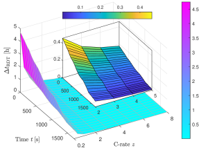
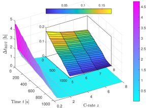
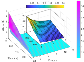
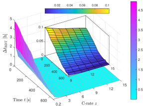
In the validation stage, we perform experiments to assess the RDE prediction for the cells. In each experiment, we discharge a cell using a variable-current profile for some time and then switch to constant-current discharging at a specified C-rate so as to determine the actual . For each cell, both the US06/SC04 profiles are used, and for each profile, four different pairs are considered. This thus involves experiments for 16 cases in total. The predicted RDT results are shown in Figs. 9-10. Figs. 11-12 compares the RDE prediction with the measurements taken from the experiments, showing a close match between them. Table 5.2 presents the quantitative comparison for all these cases. It is seen that the relative error in the RDE prediction comes less than 3% in general. We further compare our results with one traditional RDE defined as in [9]
where and are the cell’s capacity and open circuit voltage, respectively. It can be seen that has large prediction errors compared to the truth, especially at high C-rates. These results indicate that the proposed RDE prediction approach is capable of delivering high accuracy. Besides, the computational time of the proposed method is around 0.3 s when calculating the RDE for all C each time for the NCA cell and 0.4 s when calculating the RDE for all C each time for the LFP cell. This means that the update frequency of RDE at each C-rate is at least 2 Hz, which indicates that our proposed RDE prediction scheme has good computational efficiency and is applicable in real time.
6 Conclusion
RDE prediction plays an important role in managing the operation of LiBs for high safety and performance. In pursuit of this topic, we consider a new and open question: how to predict the RDE of a LiB cell if the discharging currents span from low to high C-rates? The question has emerged in some applications like electric aircraft but is nontrivial to deal with. This is because high currents will significantly impact the cell’s electro-thermal dynamics to make the RDE more difficult to identify. To address the question, we define the RDE as a C-rate-dependent quantity. With the new definition, we develop an ML approach that uses FNNs to grasp the mapping from the cell’s present state to the RDE. The approach determines the cell’s remaining discharging time due to voltage and temperature limits and then uses it along with the state to find out the RDE. To enable the training of the approach, we also develop a hybrid physics-ML model to capture the cell’s electro-thermal dynamics. The experimental validation on NCA and LFP cells shows the high prediction accuracy achieved by the proposed approach. Further, the approach is tractable for training and computationally efficient to run. It can find prospective use in different applications ranging from electric cars, heavy-duty vehicles, and aircraft to grid-scale energy storage.
Appendix. Supplement
We derive the explicit formulas for under constant and .
Letting be the initial condition, and considering that is decomposed into and . Based on (2a), the solution of is given by
which, when , becomes
| (A.11) |
It can be easily proven that has three distinct eigenvalues for . By the Cayley-Hamilton theorem, we have
| (A.12) |
where
and the operator denotes
for and . Given (A.12), the integral in (A.11) can be expressed as
| (A.13) | ||||
where . Inserting (A.12) and (6) into (A.11), we have
Similarly, we can obtain
where ,
and . Here, for are the two distinct eigenvalues of .
Acknowledgement
This work was supported in part by the National Science Foundation under Award CMMI-1847651.
References
- [1] Y. Wang, H. Fang, L. Zhou, T. Wada, Revisiting the state-of-charge estimation for lithium-ion batteries: A methodical investigation of the extended Kalman filter approach, IEEE Control Systems Magazine 37 (4) (2017) 73–96.
- [2] S. J. Moura, F. B. Argomedo, R. Klein, A. Mirtabatabaei, M. Krstic, Battery state estimation for a single particle model with electrolyte dynamics, IEEE Transactions on Control Systems Technology 25 (2) (2017) 453–468.
- [3] A. Bartlett, J. Marcicki, S. Onori, G. Rizzoni, X. G. Yang, T. Miller, Electrochemical model-based state of charge and capacity estimation for a composite electrode lithium-ion battery, IEEE Transactions on Control Systems Technology 24 (2) (2016) 384–399.
- [4] X. Lin, A. G. Stefanopoulou, Y. Li, R. D. Anderson, State of charge imbalance estimation for battery strings under reduced voltage sensing, IEEE Transactions on Control Systems Technology 23 (3) (2015) 1052–1062.
- [5] L. Hu, X. Hu, Y. Che, F. Feng, X. Lin, Z. Zhang, Reliable state of charge estimation of battery packs using fuzzy adaptive federated filtering, Applied Energy 262 (2020) 114569.
- [6] S. Zhao, S. R. Duncan, D. A. Howey, Observability analysis and state estimation of lithium-ion batteries in the presence of sensor biases, IEEE Transactions on Control Systems Technology 25 (1) (2017) 326–333.
- [7] H. Rahimi-Eichi, F. Baronti, M.-Y. Chow, Online adaptive parameter identification and state-of-charge coestimation for lithium-polymer battery cells, IEEE Transactions on Industrial Electronics 61 (4) (2014) 2053–2061.
- [8] K. Mamadou, A. Delaille, E. Lemaire-Potteau, Y. Bultel, The state-of-energy: A new criterion for the energetic performances evaluation of electrochemical storage devices, ECS Transactions 25 (35) (2010) 105.
- [9] K. L. Quade, D. Jöst, D. U. Sauer, W. Li, Understanding the energy potential of lithium-ion batteries: Definition and estimation of the state of energy, Batteries & Supercaps 6 (8) (2023) e202300152.
- [10] Y. Wang, C. Zhang, Z. Chen, An adaptive remaining energy prediction approach for lithium-ion batteries in electric vehicles, Journal of Power Sources 305 (2016) 80–88.
- [11] L. Zheng, J. Zhu, G. Wang, T. He, Y. Wei, Novel methods for estimating lithium-ion battery state of energy and maximum available energy, Applied Energy 178 (2016) 1–8.
- [12] X. Zhang, Y. Wang, J. Wu, Z. Chen, A novel method for lithium-ion battery state of energy and state of power estimation based on multi-time-scale filter, Applied Energy 216 (2018) 442–451.
- [13] L. Ma, C. Hu, F. Cheng, State of charge and state of energy estimation for lithium-ion batteries based on a long short-term memory neural network, Journal of Energy Storage 37 (2021) 102440.
- [14] G. Dong, X. Zhang, C. Zhang, Z. Chen, A method for state of energy estimation of lithium-ion batteries based on neural network model, Energy 90 (2015) 879–888.
- [15] W. Zhang, W. Shi, Z. Ma, Adaptive unscented Kalman filter based state of energy and power capability estimation approach for lithium-ion battery, Journal of Power Sources 289 (2015) 50–62.
- [16] H. He, Y. Zhang, R. Xiong, C. Wang, A novel Gaussian model based battery state estimation approach: State-of-energy, Applied Energy 151 (2015) 41–48.
- [17] G. Liu, M. Ouyang, L. Lu, J. Li, J. Hua, A highly accurate predictive-adaptive method for lithium-ion battery remaining discharge energy prediction in electric vehicle applications, Applied Energy 149 (2015) 297–314.
- [18] F. Quiñones, R. Milocco, S. Real, Remaining discharge-time prediction for batteries using the Lambert function, Journal of Power Sources 400 (2018) 256–263.
- [19] R. Xiong, Y. Zhang, H. He, X. Zhou, M. G. Pecht, A double-scale, particle-filtering, energy state prediction algorithm for lithium-ion batteries, IEEE Transactions on Industrial Electronics 65 (2) (2018) 1526–1538.
- [20] M. F. Niri, T. M. Bui, T. Q. Dinh, E. Hosseinzadeh, T. F. Yu, J. Marco, Remaining energy estimation for lithium-ion batteries via Gaussian mixture and Markov models for future load prediction, Journal of Energy Storage 28 (2020) 101271.
- [21] X.-G. Yang, T. Liu, S. Ge, E. Rountree, C.-Y. Wang, Challenges and key requirements of batteries for electric vertical takeoff and landing aircraft, Joule 5 (7) (2021) 1644–1659.
- [22] H. Tu, S. Moura, Y. Wang, H. Fang, Integrating physics-based modeling with machine learning for lithium-ion batteries, Applied Energy 329 (2023) 120289.
- [23] N. Tian, H. Fang, J. Chen, Y. Wang, Nonlinear double-capacitor model for rechargeable batteries: Modeling, identification, and validation, IEEE Transactions on Control Systems Technology 29 (1) (2021) 370–384.
- [24] X. Lin, H. E. Perez, S. Mohan, J. B. Siegel, A. G. Stefanopoulou, Y. Ding, M. P. Castanier, A lumped-parameter electro-thermal model for cylindrical batteries, Journal of Power Sources 257 (2014) 1–11.
- [25] K. Hornik, M. Stinchcombe, H. White, Multilayer feedforward networks are universal approximators, Neural Networks 2 (5) (1989) 359–366.
- [26] I. Sandberg, Global implicit function theorems, IEEE Transactions on Circuits and Systems 28 (2) (1981) 145–149.
- [27] Environmental Protection Agency, Vehicle and fuel emission testing, Technical Report.
- [28] T. M. Bandhauer, S. Garimella, T. F. Fuller, A critical review of thermal issues in lithium-ion batteries, Journal of The Electrochemical Society 158 (3) (2011) R1.