Second-order Information Promotes Mini-Batch Robustness in Variance-Reduced Gradients
Abstract
We show that, for finite-sum minimization problems, incorporating partial second-order information of the objective function can dramatically improve the robustness to mini-batch size of variance-reduced stochastic gradient methods, making them more scalable while retaining their benefits over traditional Newton-type approaches. We demonstrate this phenomenon on a prototypical stochastic second-order algorithm, called Mini-Batch Stochastic Variance-Reduced Newton (Mb-SVRN), which combines variance-reduced gradient estimates with access to an approximate Hessian oracle. In particular, we show that when the data size is sufficiently large, i.e., , where is the condition number and is the Hessian approximation factor, then Mb-SVRN achieves a fast linear convergence rate that is independent of the gradient mini-batch size , as long is in the range between and . Only after increasing the mini-batch size past this critical point , the method begins to transition into a standard Newton-type algorithm which is much more sensitive to the Hessian approximation quality. We demonstrate this phenomenon empirically on benchmark optimization tasks showing that, after tuning the step size, the convergence rate of Mb-SVRN remains fast for a wide range of mini-batch sizes, and the dependence of the phase transition point on the Hessian approximation factor aligns with our theoretical predictions.
1 Introduction
Consider the following finite-sum convex minimization problem:
| (1) |
The finite-sum formulation given in (1) can be used to express many empirical minimization tasks, where for a choice of the underlying parameter vector , each models the loss on a particular observation [31, 25, 34]. In modern-day settings, it is common to encounter problems with a very large number of observations , making deterministic optimization methods prohibitively expensive [8]. In particular, we are interested in and investigate problems where is much larger than the condition number of the problem, . In this regime (), our aim is to develop a stochastic algorithm with guarantees of returning an -approximate solution i.e., such that with high probability. As is commonly assumed in the convex optimization literature, we consider the problem setting where is -strongly convex and each is -smooth.
A prototypical optimization method for (1) is stochastic gradient descent (SGD) [26], which relies on computing a gradient estimate based on randomly sampling a single component , or more generally, a subset of components (i.e., a mini-batch). Unfortunately, SGD with constant step size does not converge to the optimal solution , but only to a neighborhood around that depends on the step size and variance in the stochastic gradient approximations. A slower sub-linear convergence rate to the optimal solution can be guaranteed with diminishing step sizes. To mitigate this deficiency of SGD, several works have explored variance reduction techniques for first-order stochastic methods, e.g., SDCA [30], SAG [28], SVRG [14], Katyusha [1] and S2GD [15], and have derived faster linear convergence rates to the optimal solution.
One of the popular first-order stochastic optimization methods that employs variance reduction is Stochastic Variance Reduced Gradient (SVRG) [14]. The method has two stages and operates with inner and outer loops. At every inner iteration, the method randomly selects a component gradient, , and couples this with an estimate of the true gradient computed at every outer iteration to compute a step. This combination, and the periodic computation of the true gradient at outer iterations, leads to a reduction in the variance of the stochastic gradients employed, and allows for global linear convergence guarantees. The baseline SVRG method (and its associated analysis) assumes only one observation is sampled at every inner iteration, and as a result, requires inner iterations in order to achieve the best convergence rate per data pass. This makes baseline SVRG inherently and highly sequential, and unable to take advantage of modern-day massively parallel computing environments. A natural remedy is to use larger mini-batches (gradient samples sizes; denoted as ) at every inner iteration. Unfortunately, this natural idea does not have the desired advantages as increasing the mini-batch size in SVRG leads to deterioration in the convergence rate per data pass. In particular, one can show that regardless of the chosen mini-batch size , SVRG requires as many as inner iterations to ensure fast convergence rate,
again rendering the method unable to take advantage of parallelization.
On the other hand, one can use stochastic second-order methods for solving (1), including Subsampled Newton [27, 6, 11], Newton Sketch [24, 3], and others [21, 20, 10, 4]. These methods use either full gradients or require extremely large gradient mini-batches at every iteration [9], and as a result, their convergence rate (per data pass) is sensitive to the quality of the Hessian estimate and to the mini-batch size . Several works [12, 13, 17, 21] have also explored the benefits of including second-order information to accelerate first-order stochastic variance-reduced methods. However, these are primarily first-order stochastic methods (and analyzed as such) resulting again in highly sequential algorithms that are unable to exploit modern parallel computing frameworks.
The shortcomings of the aforementioned stochastic methods raise a natural question, which is central to our work:
Can second-order information plus variance-reduction achieve an accelerated and robust convergence rate for a wide range of gradient mini-batch sizes?
In this work, we provide an affirmative answer to the above question. To this end, following recent prior work [9], we analyze the convergence behavior of a prototypical stochastic optimization algorithm called Mini-batch Stochastic Variance-Reduced Newton (Mb-SVRN, Algorithm 1), which combines variance reduction in the stochastic gradient, via a scheme based on SVRG [14], with second-order information from a Hessian oracle. Our Hessian oracle is general and returns an estimate that satisfies a relatively mild -approximation condition. This condition can be, for instance, satisfied by computing the Hessian of the subsampled objective (as in Subsampled Newton [27], which is what we use in our experiments), but can also be satisfied by other Hessian approximation techniques such as sketching.
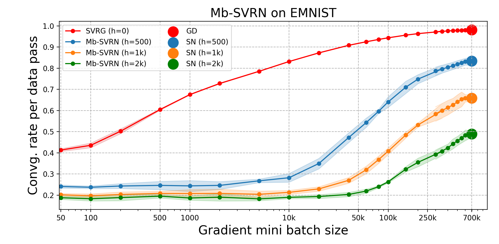
In our main result (Theorem 1) we show that even a relatively weak Hessian estimate leads to a dramatic improvement in robustness to the gradient mini-batch size for Mb-SVRN: the method is endowed with the same fast local linear convergence guarantee for any gradient mini-batch size up to a critical point , which we characterize in terms of the number of function components and the Hessian oracle approximation factor . Remarkably, unlike results for most stochastic gradient methods, our result holds with high probability rather than merely in expectation, both for large and small mini-batch sizes, and is an improvement over comparable results [9] both in convergence rate and robustness to mini-batch sizes (see Section 3). As increases beyond , the method has to inevitably transition into a standard Newton-type algorithm with a weaker convergence rate that depends much more heavily on the Hessian approximation factor . We demonstrate this phenomenon empirically on the Logistic Regression task on the EMNIST and CIFAR10 datasets (see Figure 1 and Section 5); we show that the convergence rate of Mb-SVRN indeed exhibits robustness to mini-batch size , while at the same time having a substantially better convergence rate per data pass than the Subsampled Newton method (SN) that uses full gradients. Furthermore, Mb-SVRN proves to be remarkably robust to the Hessian approximation quality in our experiments, showing that even low-quality Hessian estimates can significantly improve the scalability of the method.
Outline.
In Section 2, we provide an informal version of our main result along with a comparison with the popular SVRG and SN methods. In Section 3, we give a detailed overview of the related work in stochastic variance reduction and second-order methods. In Section 4 we present our technical analysis for the local convergence of Mb-SVRN, whereas in Theorem 4.6 we provide a global convergence guarantee. We provide experimental evidence in agreement with our theoretical results in Section 5.
2 Main Convergence Result
In this section, we provide an informal version of our main result, Theorem 5. We start by formalizing the assumptions and algorithmic setup.
Assumption 1
Consider a twice continuously differentiable function defined as in (1), where and . We make the following standard -smoothness and -strong convexity assumptions, where denotes the condition number.
-
1.
For each , is a -smooth convex function:
and is a -strongly convex function:
We also assume that the Hessians of are Lipschitz continuous.
-
2.
The Hessians of the objective function are -Lipschitz continuous:
In our computational setup, we assume that the algorithm has access to a stochastic gradient and Hessian at any point via the following gradient and Hessian oracles.
Definition 1 (Gradient oracle)
Given and indices , the gradient oracle returns such that:
We formalize this notion of a gradient oracle to highlight that the algorithm only accesses component gradients in batches, enabling hardware acceleration for the gradient computations, which is one of the main motivations of this work. We also use the gradient oracle to measure the per-data-pass convergence rate of the algorithms. Here, a data pass refers to a sequence of gradient oracle queries that access component gradients.
Definition 2 (Hessian oracle)
For an , and any , the Hessian oracle returns such that:
We refer to as the Hessian approximation factor and denote the approximation guarantee as . Here, we mention that an approximate Hessian, satisfying the above guarantee can be constructed with probability for any . We deliberately do not specify the method for obtaining the Hessian estimate, although in the numerical experiments we will use a sub-sampled Hessian estimate of the form , where the sample size controls the quality of the Hessian approximation (e.g., as in Figure 1). We treat the cost of Hessian approximation separate from the gradient data passes, as the complexity of Hessian estimation is largely problem and method dependent. Naturally, from a computational stand-point, larger generally means smaller Hessian estimation cost.
2.1 Main algorithm and result
In this section, we present an algorithm that follows the above computational model (Algorithm 1, Mb-SVRN), and provide our main technical result, the local convergence analysis of this algorithm across different values of the Hessian approximation factor and gradient mini-batch sizes . We note that the algorithm was deliberately chosen as a natural extension of both a standard stochastic variance-reduced first-order method (SVRG) and a standard Stochastic Newton-type method (SN), so that we can explore the effect of variance reduction in conjunction with second-order information on the convergence rate and robustness.
We now informally state our main result, which is a local convergence guarantee for Algorithm 1 (for completeness, we also provide a global convergence guarantee in Theorem 4.6). In this result, we show a high-probability convergence bound, that holds for gradient mini-batch sizes as small as and as large as , where the fast linear rate of convergence is independent of the mini-batch size.
Theorem 1 (Main result; informal Theorem 5)
Remark 1
Under our assumption that , the convergence rate satisfies , i.e., it is a fast condition-number-free linear rate of convergence that gets better for larger data sizes . Since we used , one outer iteration of the algorithm corresponds to roughly two passes over the data (as measured by the gradient oracle calls).
2.2 Discussion
Our convergence analysis in Theorem 1 shows that incorporating second-order information into a stochastic variance-reduced gradient method makes it robust to increasing the gradient mini-batch size up to the point where . This is illustrated in Figure 2 (compare to the empirical Figure 1), where the robust regime corresponds to the convergence rate staying flat as we vary . Improving the Hessian oracle quality (smaller ) expands the robust regime, allowing for even larger mini-batch sizes with a flat convergence rate profile.
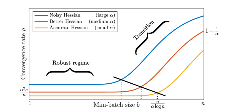
Note that, unless is very close to (extremely accurate Hessian oracle), the convergence per data pass must eventually degrade, reaching , which is the rate achieved by the corresponding Newton-type method with full gradients (e.g., see Lemma 2). The transition point of arises naturally in this setting, because the convergence rate after one outer iteration of Mb-SVRN could not be better than where (obtained by treating the stochastic gradient noise as negligible).
Implications for stochastic gradient methods.
In the case where the Hessian oracle always returns the identity, Mb-SVRN reduces to a first-order stochastic gradient method which is a variant of SVRG [14]. So, it is natural to ask what our convergence analysis implies about the effect of second-order preconitioning on an SVRG-type algorithm. In our setting, SVRG with mini-batch size achieves an expected convergence rate of , compared to a high-probability convergence rate of for Mb-SVRN. This means that, while for small mini-batches the advantage of preconditioning is not significant, the robust regime of Mb-SVRN (which is not present in SVRG) leads to a gap in convergence rates between the two methods that becomes larger as we increase (see Figure 1). This suggests the following general rule-of-thumb:
To improve the robustness of an SVRG-type method to the gradient mini-batch size, one can precondition the method with second-order information based on a Hessian estimate.
Implications for Newton-type methods.
A different perspective on our results arises if our starting point is a full-gradient Newton-type method, such as Subsampled Newton [27] or Newton Sketch [24], which also arises as a simple corner case of Mb-SVRN by choosing mini-batch size and inner iterations . In this setting, as mentioned above, the convergence rate of the method behaves as , which means that it is highly dependent on the quality of the Hessian oracle via the factor . As we decrease in Mb-SVRN, the method gradually transitions into an SVRG-type method that is more robust to Hessian quality. We note that while our theoretical convergence result in Theorem 1 still exhibits a dependence on , empirical results suggest that for large datasets this dependence is much less significant in the robust regime of Mb-SVRN than it is in the full-gradient regime. This suggests the following general prescription:
To improve the robustness of a Newton-type method to the Hessian estimation quality, one can replace the full gradients with variance-reduced sub-sampled gradient estimates.
3 Related Work
Among first-order methods, [30] propose SDCA, a stochastic variant of dual coordinate ascent. In [29], the SAG algorithm is proposed, which maintains in memory the most recent gradient value computed for each training example, updates the gradient value by selecting a random sample at every iteration, and computes the average gradient. Both SDCA and SAG achieve convergence guarantees comparable to those of SVRG (see Section 2.2). In [34], the authors propose a variant of SVRG, called Prox-SVRG for minimizing the sum of two convex functions, and , where takes the form as in (1) and is a regularizer. They leverage the composite structure of the problem and incorporate a weighted sampling strategy to improve the complexity so that it depends on the so-called average condition number, , instead of . We note that a similar weighted sampling strategy can be incorporated into Mb-SVRN with little additional effort. On the other hand, methods such as Katyusha [1, 2] and Catalyst [16] use Nesterov-type techniques to accelerate SVRG and achieve improved convergence guarantees where the condition number is replaced by its square root . In particular, Catalyst [16] adds a strongly convex penalty term to the objective function at every iteration, and solves a sub-problem followed by introducing momentum. That said, similar to SVRG, all methods discussed in this paragraph are first-order methods and the convergence rate (per data pass) of these methods is not robust to the gradient mini-batch size.
To this end, methods that incorporate stochastic second-order information have been proposed. In [12], using similar approaches to those in [34], a sketched preconditioned SVRG method is proposed, for solving ridge regression problems, that reduces the average condition number of the problem. The works [13, 18, 21], employ L-BFGS-type updates to approximate the Hessian inverse which is then used as a preconditioner to variance-reduced gradients. In [17], the authors proposed an inexact preconditioned second-order method. All these methods are inherently first-order methods that use preconditioning to improve the dependence of SVRG-type methods on the condition number, and for practical considerations. In particular, their existing convergence analyses do not show scalability and robustness to gradient mini-batch sizes.
Popular stochastic second-order methods, e.g., Subsampled Newton [27, 6, 11] and Newton Sketch [24, 3], either use the full gradient or require extremely large gradient mini-batch sizes at every iteration [9]. As a result, the convergence rate of these methods depends heavily on the quality of Hessian approximation, and the methods are unsuitable for implementations with low computational budget. Several other works have used strategies to reduce the variance of the stochastic second-order methods. One such work is Incremental Quasi-Newton [20] which relies on memory and uses aggregated gradient and Hessian information coupled with solving a second-order Taylor approximation of in a local neighborhood around in order to reduce the variance of stochastic estimates employed. In [7] the authors propose methods that combine adaptive sampling strategies to reduce the variance and quasi-Newton updating to robustify the method. Finally, in [22] the authors show that averaging certain types of stochastic Hessian estimates (such as those based on subsampling) results in variance reduction and improved local convergence guarantees when used with full gradients. Unfortunately, the convergence rates of these methods are not robust to the sample size used for computing the stochastic gradients and/or the quality of Hessian approximation. Also, we note that these methods update the Hessian approximations at every iteration and are not directly comparable to our setting in which we update the Hessian approximation using a multi-stage approach.
Recently, [9] investigated the effect of variance-reduced gradient estimates in conjunction with a Newton-type method, using an algorithm comparable to Mb-SVRN. They show that using gradient mini-batch size of the order , one can achieve a local linear convergence rate of . However, deviating from this prescribed mini-batch size (in either direction) causes the local convergence guarantee to rapidly degrade, and in particular, the results are entirely vacuous unless . Our work can be viewed as a direct improvement over this prior work: first, through a better convergence rate dependence on (with versus ); and second, in showing that this faster convergence can be achieved for any mini-batch size . We achieve this by using a fundamentally different analysis via a chain of martingale concentration arguments combined with using much smaller step sizes in the inner iterations, which allows us to compensate for the additional stochasticity in the gradients in the small and moderate mini-batch size regimes.
4 Convergence Analysis
In this section, we present our technical analysis that concludes with the main convergence result, Theorem 5, informally stated earlier as Theorem 1. We start by introducing some auxiliary lemmas in Section 4.1. Then, in Theorem 2 (Section 4.2), we establish a one inner iteration convergence result in expectation, forming the key building block of our analysis. Then, in Section 4.3, we present our main technical contribution; we construct a submartingale framework with random start and stopping times, which is needed to establish fast high-probability linear convergence of outer iterates in Theorem 5, our main convergence result (Section 4.5). At the end of this section, we supplement our main local convergence results with a global convergence guarantee for Mb-SVRN in Theorem 6 (Section 4.6).
Notation.
Let denote the starting outer iterate and denote the outer iterate after outer iterations. Within the outer iteration, the inner iterates are indexed as . Since our results require working only within one outer iteration, we drop the subscript throughout the analysis, and denote as and corresponding inner iterate as . Similarly let and denote the Hessian at and , respectively. For gradient mini-batch size , let denote , let denote and let denote the variance-reduced gradient at , where represents exact gradient at . Moreover, represents exact gradient at , represents Hessian at , and let , . Also, we use to denote the fixed step size. Finally, we refer to as the conditional expectation given the event that the algorithm has reached iterate starting with the outer iterate .
Next, we define the local convergence neighborhood, by using the notion of a Mahalanobis norm: , for any positive semi-definite matrix and vector .
Definition 3
For a given , we define a local neighborhood around , as follows:
where is the Lipschitz constant for Hessians of , and is the strong convexity parameter for .
4.1 Auxiliary lemmas
In this section we present auxiliary lemmas that will be used in the analysis. The first result upper bounds the variance of the SVRG-type stochastic gradient in terms of the smoothness parameter and gradient mini-batch size . Similar variance bounds have also been derived in prior works [14, 9, 5].
Lemma 1 (Upper bound on variance of stochastic gradient)
Let and for some . Then:
Proof
Refer to Appendix A.1.
In the following result, we use standard approximate Newton analysis to establish that, using an -approximate Hessian at (Definition 2, denoted as ), a Newton step with a sufficiently small step size reduces the distance to (in norm), at least by a factor of . We call this an approximate Newton step since the gradient is exact and only the second-order information is stochastic.
Lemma 2 (Guaranteed error reduction for approximate Newton)
Consider an approximate Newton step where , , , and , for some , and . Then:
where denotes the Hessian matrix at .
Proof
Refer to Appendix A.2.
Note that the approximate Newton step in Lemma 2 uses an exact gradient at every iteration, requiring the use of all data samples. In our work, in addition to approximate Hessian, we incorporate variance-reduced gradients as well, calculated using samples out of . For a high probability analysis, we require an upper bound on the noise introduced due to the stochasticity in the gradients. The next result provides an upper bound on the noise (with high probability) in a single iteration introduced due to noise in the stochastic gradient.
Lemma 3 (High-probability bound on stochastic gradient noise)
Let , , , . Then, for any , with probability at least (depending on the gradient mini-batch size ):
Proof
Refer to Appendix A.3.
The next result provides an upper bound on the gradient in terms of the distance of to the minimizer . The result is useful in establishing a
lower bound on in terms of , essential to control the randomness in our submartingale framework, described in later sections.
Lemma 4 (Mean Value Theorem)
Let , for . If the Hessian estimate satisfies , then
Proof
Refer to Appendix A.4.
4.2 One step expectation result
In the following theorem, we use the auxiliary lemmas (Lemma 1 and Lemma 2) to show that for a sufficiently small step size , in expectation, Mb-SVRN is similar to the approximate Newton step (Lemma 2), with an additional small error term that can be controlled by the step size . We note that while this result illustrates the convergence behavior of Mb-SVRN, it is by itself not sufficient to guarantee overall convergence (either in expectation or with high probability), because it does not ensure that the iterates will remain in the local neighborhood throughout the algorithm (this is addressed with our submartingale framework, Section 4.3).
Theorem 2 (One inner iteration conditional expectation result)
Let , , . Consider Mb-SVRN with step size and gradient mini-batch size . Then:
Proof Taking the conditional expectation of ,
This is because and therefore the cross term vanishes. Since we know that and , by Lemma 2 we have . Substituting this in the previous inequality, it follows that
Using that and , we have . Therefore, . So we get,
Upper bounding ,
By Lemma 1, we bound the last term of the previous inequality,
Putting it all together,
| (2) |
where we used that and imply
.
In the remainder of the
analysis, we set and consider for some . These specific values for and are set in hindsight based on the optimal step size and the neighborhood scaling factor derived later as artifacts of our analysis. On the other hand, one can do the analysis with general and and later derive these assignments for and . The value for also gets specified as the analysis proceeds.
4.3 Building blocks for submartingale framework
We begin by building an intuitive understanding of our submartingale framework, where we define a random process to describe the convergence behavior of the algorithm. Informally, one can think of as representing the error , and aiming to establish the submartingale property . We next highlight two problematic scenarios with achieving the submartingale property, which are illustrated in Figure 3.
First, the assumption in Theorem 2 ensures that the approximate Newton step reduces the error at least by a factor of . However, if , this claim is no longer valid, leading to the first scenario that disrupts the submartingale behavior. This implies the necessity of the property , for some constant , to establish . In the course of our martingale concentration analysis, we show the existence of an absolute constant , such that , for all , with high probability.
We now explain the second scenario that disrupts the submartingale property. Note that, involves noise arising due to the stochasticity of the variance-reduced gradient . This stochasticity leads to the term in the statement of Theorem 2. Now, in the event that this noise dominates the error reduction due to the approximate Newton step, one cannot establish that . This problematic scenario occurs only when , i.e., when the error becomes small enough to recover our main convergence guarantee. As the algorithm cannot automatically detect this scenario and restart a new outer iteration, it still performs the remaining inner iterations. This results in subsequent inner iterates being affected by high stochastic gradient noise, disrupting the submartingale property.
To address these scenarios, we introduce random stopping times and random resume times , where stopping times capture the disruptive property scenarios, and resume times capture property restoration after encountering stopping times. Refer to Figure 3 for a visual representation, where the dashed curve denotes the error , the -axis denotes the iteration index , denotes the stopping time, and denotes the resume time. The submartingale property holds as long as stays between the brown and blue lines (i.e., in the white strip between the grey ). The brown line at the top denotes the scenario where , and the blue line at the bottom denotes the scenario where . The green line denotes the convergence guarantee provided in our work, which remarkably is a constant multiple of the blue line. Our martingale concentration argument shows that after iterations, the error will, with high probability, fall below the green line.
We proceed to formally define the random stopping and resume times. Consider a fixed . Define random stopping times and random resume times , with and for , as
| (3) |
The random stopping time denotes the iteration index when the random sequence leaves the local neighborhood or satisfies . The random resume time denotes the iteration index when the random sequence returns back to the local neighborhood and also satisfies . The condition , ensures that the previous results (Lemma 1, 2, 3) hold with , whereas the condition , captures the fact that the optimal convergence rate has not been achieved at . These two different conditions are required to design a submartingale from random time to . Note that, in hindsight, we have defined stopping time in a way similar to our convergence guarantee, . We add a factor to capture constants and log factors that can appear in the convergence guarantee. One can show that for , the behavior of is dictated by the variance in the stochastic gradient and not the progress made by the approximate Newton step.
Remark 2
The stopping and resume times satisfy the following properties:
-
(a)
For , we have . This is due to the definitions of and in (3). Equivalently, we can write,
(4) -
(b)
For and given that , we have . This is because is the first instance after such that . Equivalently, we can write,
(5) -
(c)
For any gradient mini-batch size , Mb-SVRN performs inner iterations, and therefore by construction random times and would not be realized more than times.
Note that due to (5), Mb-SVRN provides a very strong guarantee on the error of the iterates when and . However, the stopping time can be realized due to or , and in that case the conditioning event in (5) may never hold.
Now we proceed to construct a submartingale framework from the random resume time to the random stopping time . Our aim is to apply Freedman’s inequality on a carefully constructed martingale and prove strong concentration guarantees on , resulting in our main result. We state a version of Freedman’s inequality for submartingales (which is a minor modification of standard Freedman’s for martingales [32], see Appendix A.5).
Theorem 3 (Freedman’s inequality for submartingales)
For a random process satisfying and , it follows that:
As required for the application of Freedman’s inequality on any random process, we need to establish the following three properties:
-
(a)
the submartingale property, i.e., ;
-
(b)
the predictable quadratic variation bound, i.e., a bound on ;
-
(c)
and the almost sure upper bound, i.e., a bound on .
The next lemma shows that if lies in the local neighborhood , and does not satisfy , then we have a submartingale property ensuring that in expectation is smaller than .
Lemma 5 (Submartingale property till stopping time)
Let the gradient mini-batch size be and . Let , , , , and . Then:
Remark 3
We make a few remarks about the step size which comes out of our analysis as the optimal choice. Lemma 5 requires that , where the first term in the bound ensures convergence of the approximate Newton step, whereas the second term guarantees control over the gradient noise. In the regime where (which we assume in our main result), it is always true that our chosen step size satisfies . However, to ensure that we must restrict the mini-batch size to . In our main result, we use . This suggests that, in the regime of , the choice of the step size is primarily restricted by the Hessian approximation factor . Ultimately, this leads to deterioration of the convergence rate as increases beyond .
Throughout our analysis, we assume , which corresponds to the condition stated informally in Theorem 1. This is the regime where the convergence rate of Mb-SVRN does not deteriorate with . Having established the submartingale property, we now prove the predictable quadratic variation bound property. For proving a strong upper bound on the quadratic variation, we need a result upper bounding by , as long as the stopping time criteria are not satisfied at .
Lemma 6 (Bounded variation)
Let with and . Also, let and for some . Then, with :
Proof We apply Jensen’s inequality to to get,
Since , we have . By using Lemma 4 on the term ,
The last inequality holds because . Finally, we use the condition that , concluding the proof.
We proceed with the predictable quadratic variation bound for , assuming that does not satisfy the stopping time criteria.
Lemma 7 (Predictable quadratic variation bound)
Let with and for some . Also, let and for some . Then, with :
Proof Consider . We have,
Using and , we get,
Using Jensen’s inequality on the first term, we have , from which it follows that,
| (6) |
Using the fact that and , we have . Therefore, . Combining this with the inequality (6),
Upper bounding , we get,
| (7) |
Since , we have . By using Lemma 1 on the last term of the inequality (7), it follows that,
| (8) |
Substituting (8) in the inequality (7), we get,
Again, using ,
Since , we use Lemma 6 on to obtain,
Substituting one of the factors as , and , concludes the proof.
Finally, as the last building block of the submartingale framework, we establish a high probability upper and lower bound on in terms of . Here, due to the noise in the stochastic gradient, we cannot prove almost sure bounds. However, by Lemmas 3 and 6, we can get the upper and lower bounds, holding with probability at least , for any . For notational convenience, we use to denote the high probability upper bound on , guaranteed in Lemma 3,
Lemma 8 (One step high probability upper bound)
Let , with , and , for some , , and any . Also, let and . Then, with , and probability at least :
Proof We first prove the right-hand side inequality (upper bound),
Since, and , we have , and therefore, . Using this we get,
Note that the first term is . Also as , we have , and therefore, we can apply Lemma 3 on the second term. As captures the effect of whether or , we have with probability at least ,
By it follows that,
and using Lemma 6, we upper bound by and get,
| (9) |
Next, we prove the left-hand side inequality (lower bound), observing that,
Note that,
Using Lemma 1 to upper bound and substituting in the previous inequality for , we get,
Now in the last term, we use and upper bound the second term using Lemma 3. Following the same steps as we did for the right-hand side inequality, we get
Using Lemma 6 on ,
implying,
By the condition on , namely , it follows that,
| (10) |
4.4 Martingale setup
In what follows, we analyze the behavior of a carefully defined random process from random times to , for . In particular, we show that if then with very high probability for some absolute constant , and if then with very high probability. For any , such that , we consider an event ,
The event captures the occurrence of the high probability event mentioned in Lemma 3, for iterates ranging from random time to . Using Lemma 3, it follows that , and by the union bound . Consider a random process defined as:
and for ,
where means expectation conditioned on the past till iterate . At iteration , the random process checks for the two halting conditions mentioned in the definition of . If any of the halting condition is met then we get , the random process halts, otherwise, the random process proceeds to iteration . We analyze the random process till . The first observation is that is a sub-martingale, proven as follows. If or then and trivially . So we consider and get,
| (11) |
Due to the quadratic variation bound Lemma 7, for we have,
| (12) |
We use (12) to upper bound , where denotes the expectation conditioned on the past and assuming is known. First note that if or , then , and therefore . Hence, it remains to consider the case when ,
Note that in the event of , by Lemma 8 we know that , assuming that and satisfy the assumptions of Lemma 8. Consider the following inequality for such that ,
With and , we use the above inequality to get,
where the last inequality is due to (12). Thus, we get the following predictable quadratic variation bound for random process ,
| (13) |
Now we aim to upper bound for such that . Again, in the events or , we have and we are done. Considering the case ,
Again due to having , we invoke Lemma 8 to get,
where , and
Similarly, we get,
Combining the above upper bound property with (11) and (13), we get the following submartingale framework.
Lemma 9 (Submartingale setup)
Let , , and for some and . Consider the random process defined as , and for ,
Then, letting :
4.5 High probability convergence via martingale framework
In the previous section, we constructed a submartingale framework satisfying a quadratic variation bound and high probability upper bound at every step. In this section, we invoke a well-known measure concentration result for martingales, Freedman’s inequality stated in Theorem 3, on our framework. We apply Theorem 3 on the random process . For brevity, we provide the analysis only for the case . This means replacing by in Lemma 9. The proof for the case follows along the similar line, by replacing with .
We consider , , fix , and apply Freedman’s inequality on the random process until does not satisfy any of stopping time criteria mentioned in the definition of , (3). Consider two cases here,
Case 1: . Note that
where in the last inequality we use and . We get,
where last inequality holds if .
Case 2: . Note that
where in the last inequality we use . We get,
Substitute and , we get,
Letting , we get the failure probability less than . Combining both cases, we get the following powerful concentration guarantee.
Theorem 4 (Freedman’s concentration)
Let , , , and . Then, for any satisfying :
where , with probability at least .
Proof By Theorem 3, we have with probability at least . This implies,
| (14) |
Since , we have and also . By Lemma 3, and applying the union bound for inner iterations starting from we have . Combining this with (14) and rescaling by a factor of , we get with probability at least ,
By Lemma 5, with , we have , for any such that . So, with probability at least ,
which concludes the proof.
Remark 5
The next two results show that for any stopping time , with high probability, and, moreover, if then . We start by proving the result for the first stopping time .
Lemma 10 (High probability result for first stopping time)
Proof By conditioning on the first stopping time, whether or , and using law of total probability, it follows that,
Note that we bound the second term above by (17). We proceed to bound the first term. Consider the submartingale running till stopping time . If , then this implies that the submartingale continued for the full outer iteration. We apply the result of Theorem 4 on to get, with probability at least ,
which implies,
For and , it follows that ,
which concludes the proof.
Since there can be more than one stopping time, we prove a result similar to Lemma 10 for stopping times occurring after the first stopping time. Note that this requires conditioning on the previous stopping time. As we already have an unconditional high probability result for in Lemma 10, having conditioning on previous stopping time allows us to establish a high probability result for any subsequent stopping time.
Lemma 11 (High probability result for non-first stopping time)
Proof First, note that as , we have . Now due to one step high probability bound in Lemma 8 we have . Similar to Lemma 10 we show that,
| (18) |
and,
| (19) |
Now we invoke the Freedman concentration result Theorem 4 on the sub-martingale , to get with probability at least ,
proving that
Note that this condition does not depend on the value of . In particular, for we get,
establishing the inequality (18). Next, to prove the inequality (19), observe that implies that either or . We have already shown that with probability at least ,
Combining this with we get,
obtaining that
which concludes the proof.
Note that for the and values prescribed in Lemma 10 and the lower bound on from Theorem 4, a sufficient condition on can be stated as: for . We are now ready to prove our main convergence result.
Theorem 5 (High probability convergence over outer iterates)
Let , and . Let , and . Then with probability at least :
for absolute constants and .
Proof Note that in our running notation, is just . We prove one outer iteration result where means . Consider and and note that due to our assumptions, the results of Theorem 4 and Lemmas 10 and 11 hold. Also for the given values of and , the upper bound condition on can be replaced with , where . Let be the event denoting our convergence guarantee, i.e.,
Also we define events for all as following,
Due to Lemma 11 we know that . Moreover, by using the law of total probability in conjunction with conditioning on the first stopping time, we have,
Using Lemma 10, we have , and
| (20) |
Next, we consider the term ,
By Lemma 10, . Substituting this in (20),
| (21) |
We now show that for any . Consider the following,
By Lemma 11, we have ,
| (22) |
We write as follows,
where in the last inequality we use . We also use Lemma 11 to write , implying,
| (23) |
Substituting (23) in (22), we get,
Since we perform a finite number of iterations, for any . This intuitively means that the number of stopping times is upper bounded by the number of inner iterations. In the worst case , which means that for . implying that . Also note that if for some integer , then . Combining this with the fact there cannot be more than stopping times, along with using (21) we get,
Incorporating the total failure probability of Lemma 3 for any of the iterations, we get a failure probability of at most .
As a final step, we prove our result in terms of function values. Since has continuous first- and second-order derivatives, by the quadratic Taylor expansion, for vectors and , there exists a such that,
Let , ,
With high probability, we know that and have . Take , we have . Then,
so it follows that,
Using the reverse inequality with in place of , we have,
Combining the above two relations with the definition of , we get with probability at least ,
Setting , and writing the result in terms of outer iterates by noticing and , concludes the proof.
4.6 Global convergence analysis
In this section, we prove the global convergence of Mb-SVRN. Unlike Theorem 5 we have no local neighborhood condition and we do not put any condition on the gradient mini-batch size. Due to being a stochastic second-order method, the global rate of convergence of Mb-SVRN is provably much slower than the local convergence guarantee.
Theorem 6 (Global convergence of Mb-SVRN)
For any gradient mini-batch size and there exists such that,
Proof
Refer to Appendix A.6.
5 Numerical Experiments
We now present more extensive empirical evidence to support our theoretical analysis. We considered a regularized logistic loss minimization task with two datasets, EMNIST dataset () and CIFAR10 dataset () transformed using a random feature map obtaining features for both datasets. In addition to the above two datasets, we performed experiments on a logistic regression task with synthetic data (with , ); see Appendix B.
5.1 Experimental setup
The regularized logistic loss function can be expressed as the following finite-sum objective function:
where denote the training examples with and for . The function is -strongly convex. We set in our experiments on EMNIST and CIFAR10. Before running Mb-SVRN, for all datasets, we find the respective to very high precision by using Newton’s Method. This is done in order to calculate the error at every iteration . For the Hessian approximation in Mb-SVRN, we use Hessian subsampling, e.g., as in [27, 6], sampling component Hessians at the snapshot vector and constructing . The algorithmic implementation is discussed in Algorithm 1. For every combination of gradient mini-batch size (), step size () and Hessian sample size () chosen for any particular dataset, we tune the number of inner iterations to optimize the convergence rate per data pass and take the average over runs. We run the experiments for a wide range of step size values in the interval .
We compute the convergence rate per data pass experimentally with an approximation scheme described in this section. First, note that one full data pass is done at the start of the outer iteration to compute . Thereafter, for chosen gradient mini batch-size , component gradients are computed at every inner iteration ( component gradients each for and , respectively). Thus, after inner iterations the number of data passes is given as:
Once we have the number of data passes , we can compute the convergence rate per data pass at inner iterate as the following:
where is the inner iterate and is the outer iterate. Since it is infeasible to find at every inner iterate with an aim to find that minimizes , we use the following an approximation scheme.
We calculate the convergence rate per data pass () once after every inner iterations. If our calculations yield that has increased twice continuously or the method starts diverging , we halt and return the minimum value of recorded thus far. Furthermore, for very large values of , we increase the frequency of computing (compute after every inner iterations). In the following sections, we discuss the robustness of Mb-SVRN to gradient mini-batch size and step size.
5.2 Robustness to gradient mini-batch size

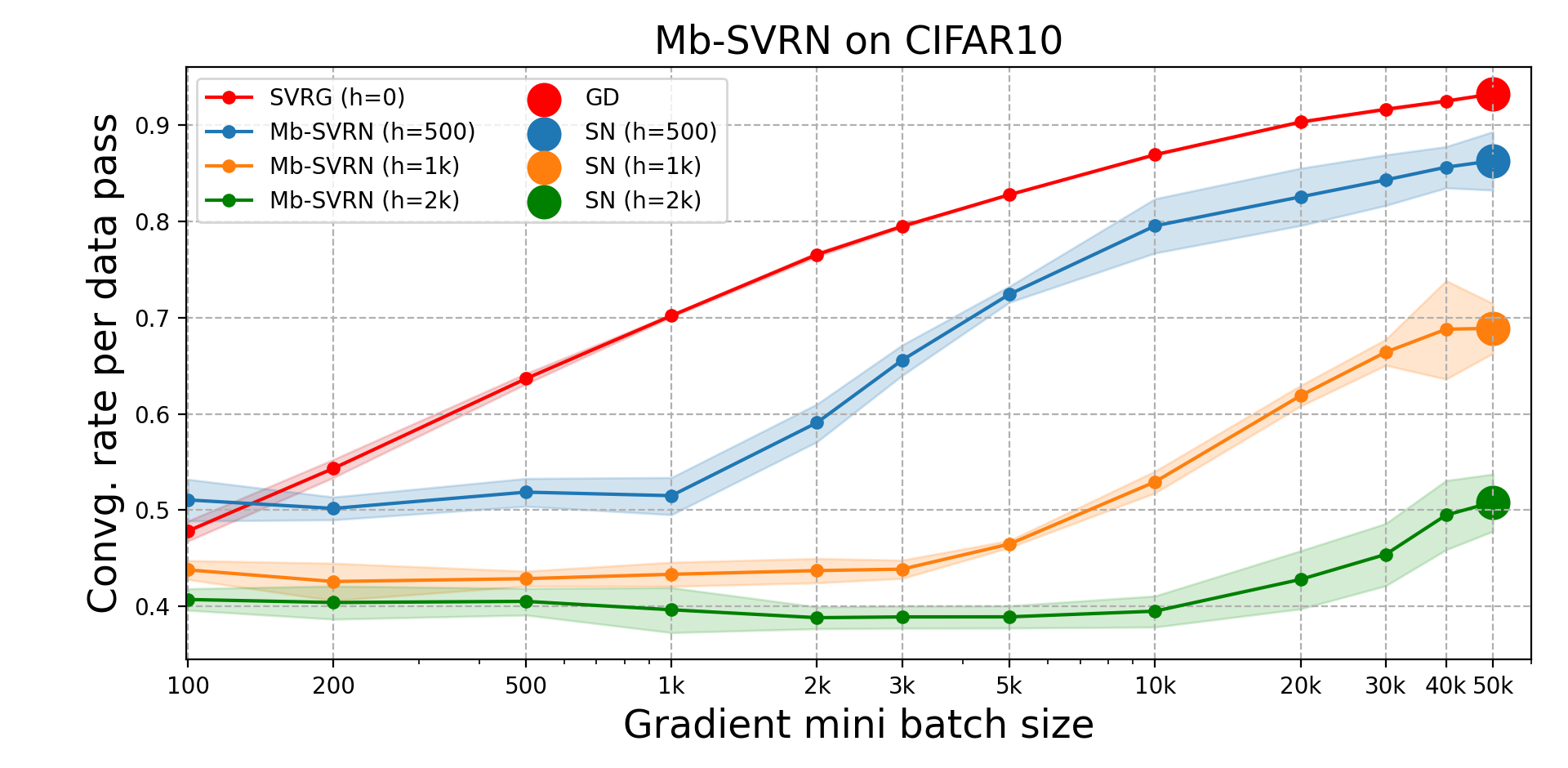
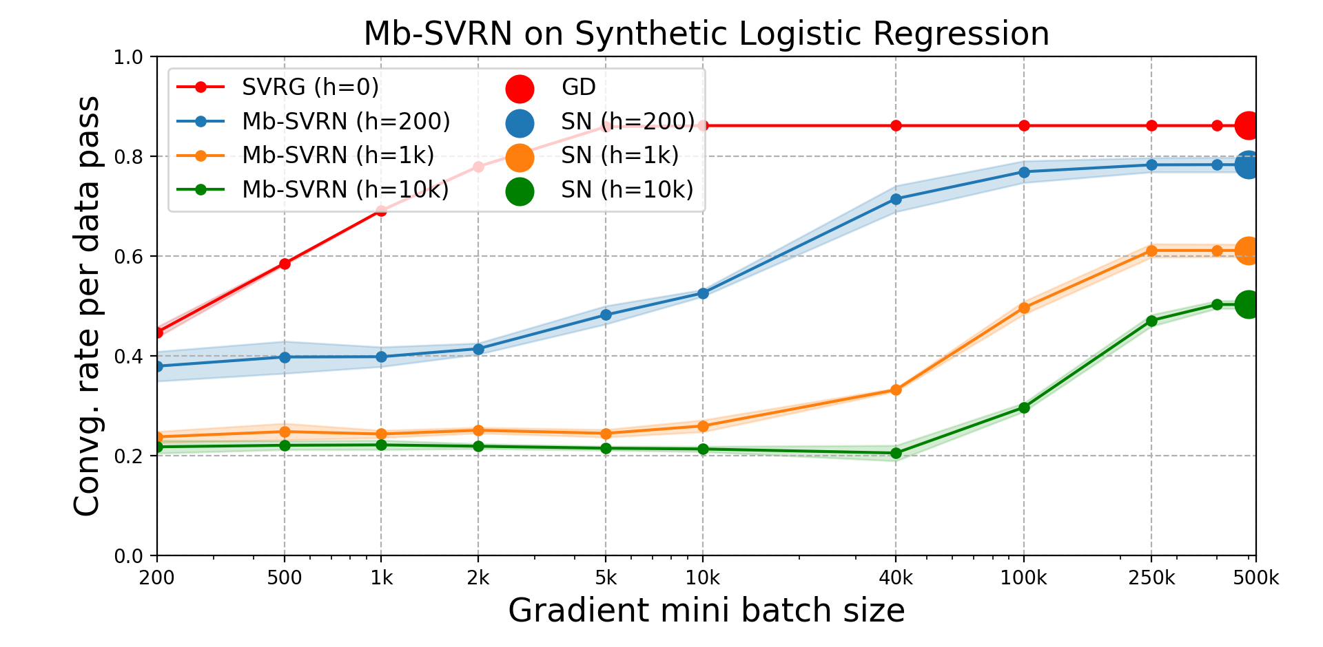
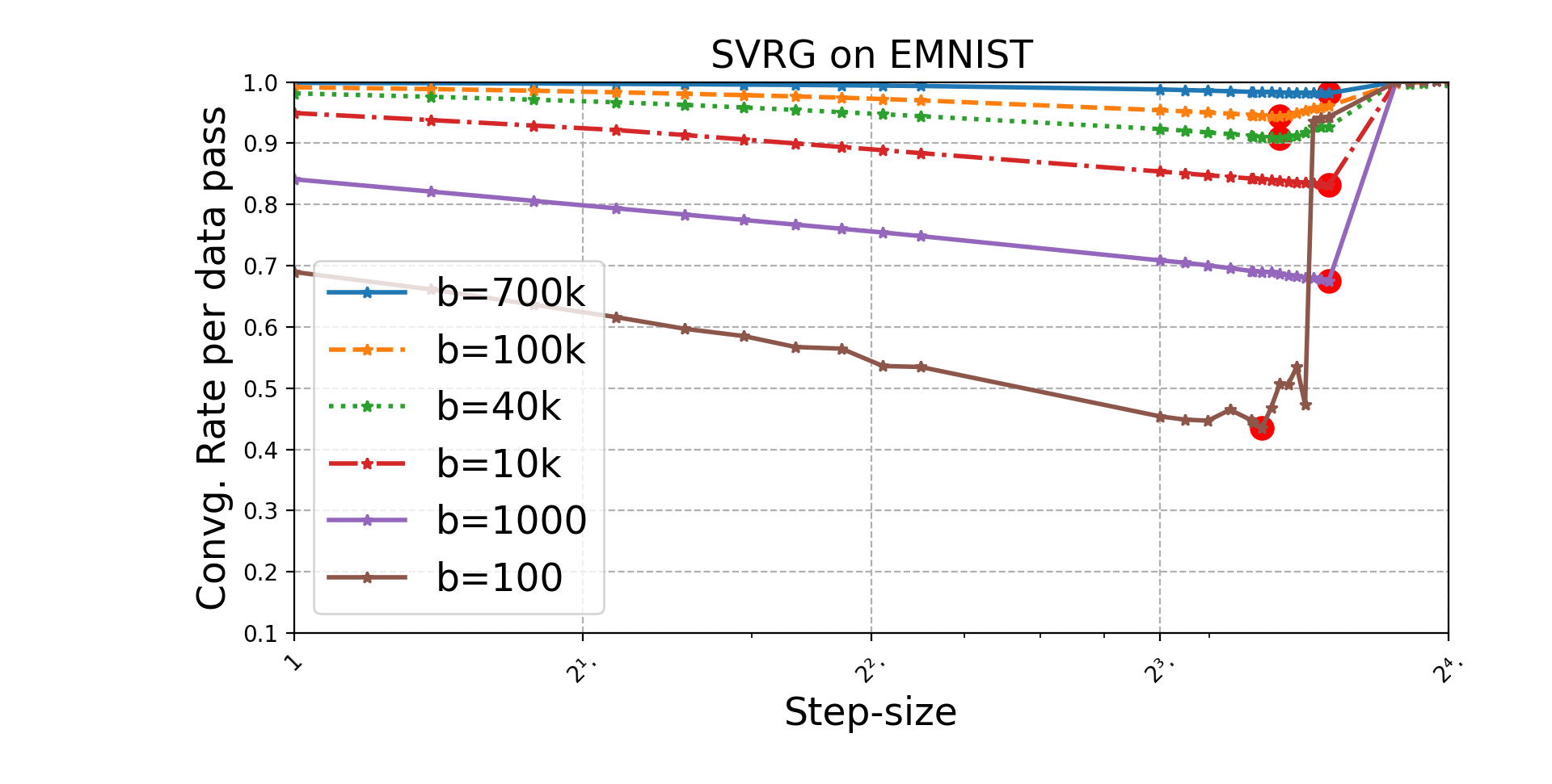
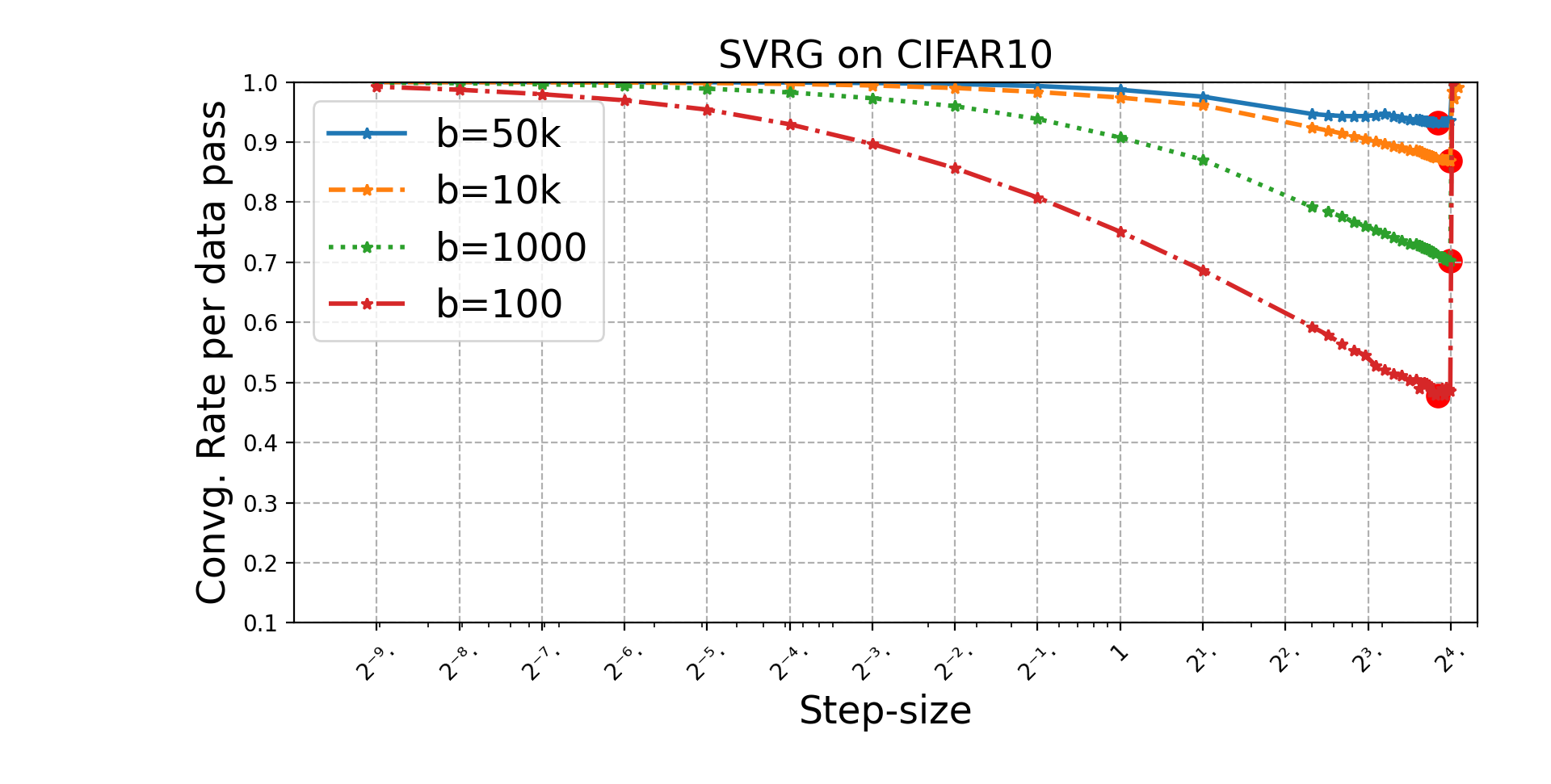
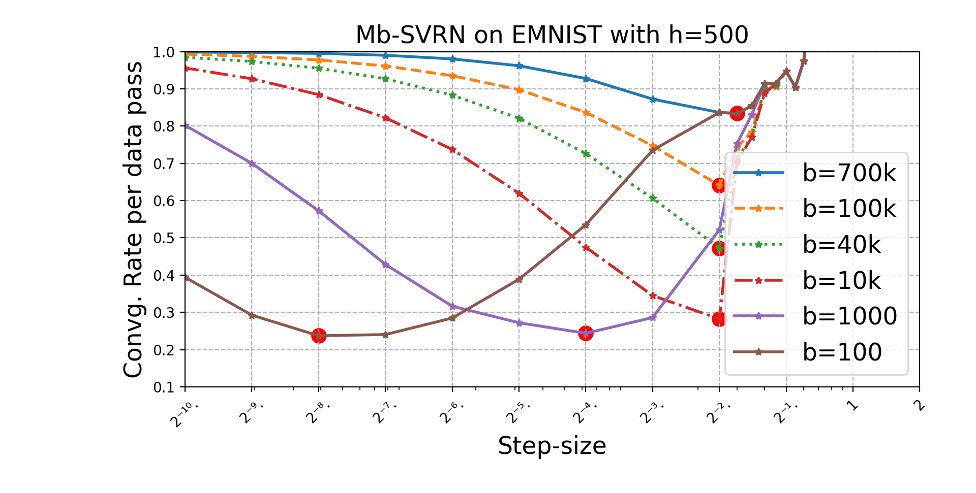
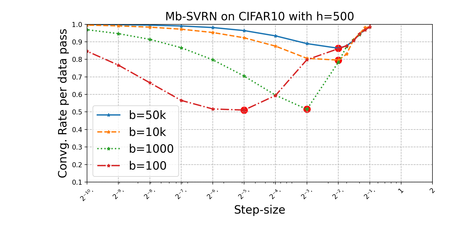
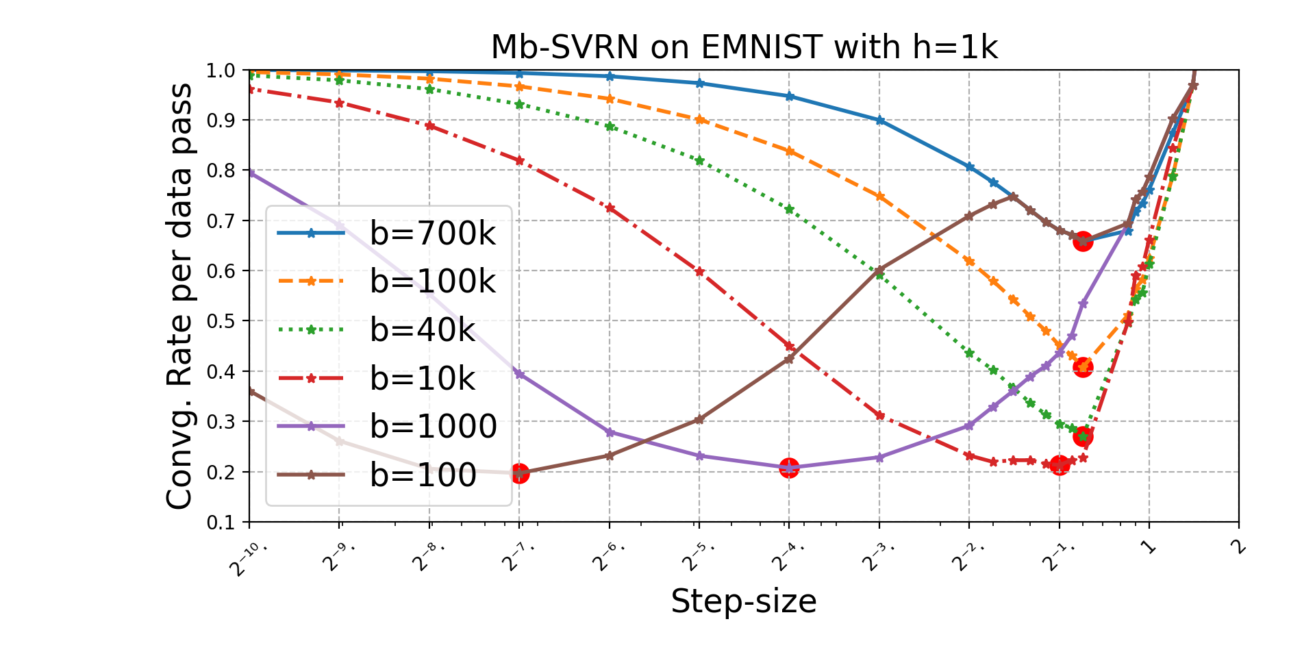
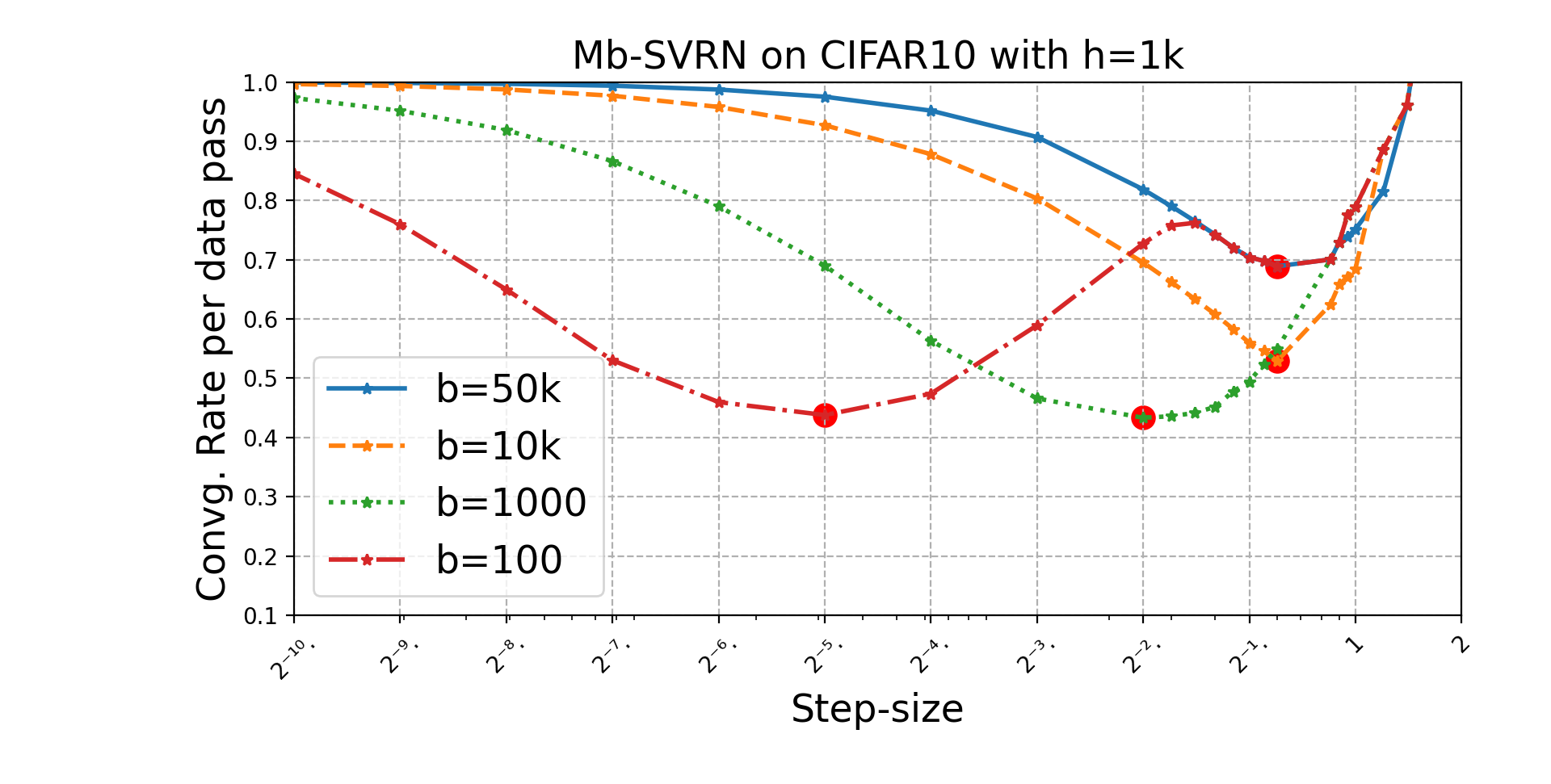
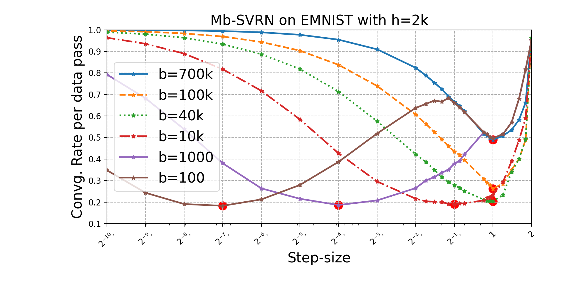
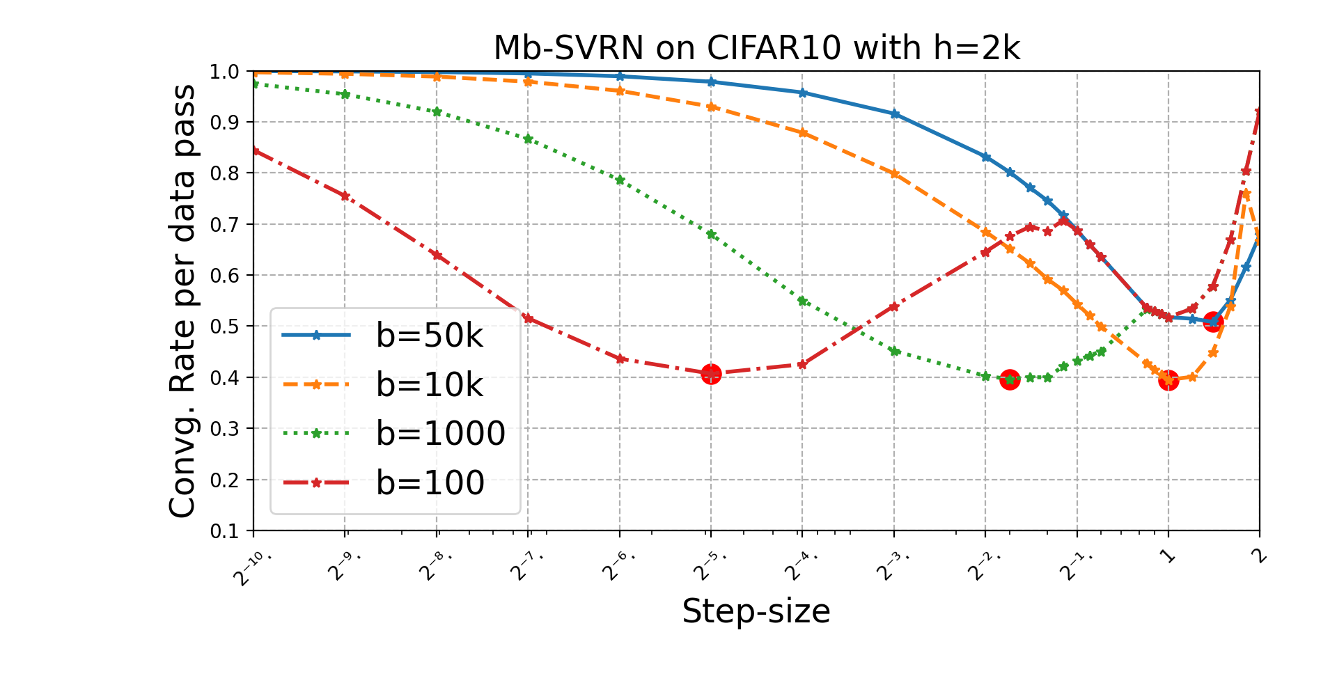
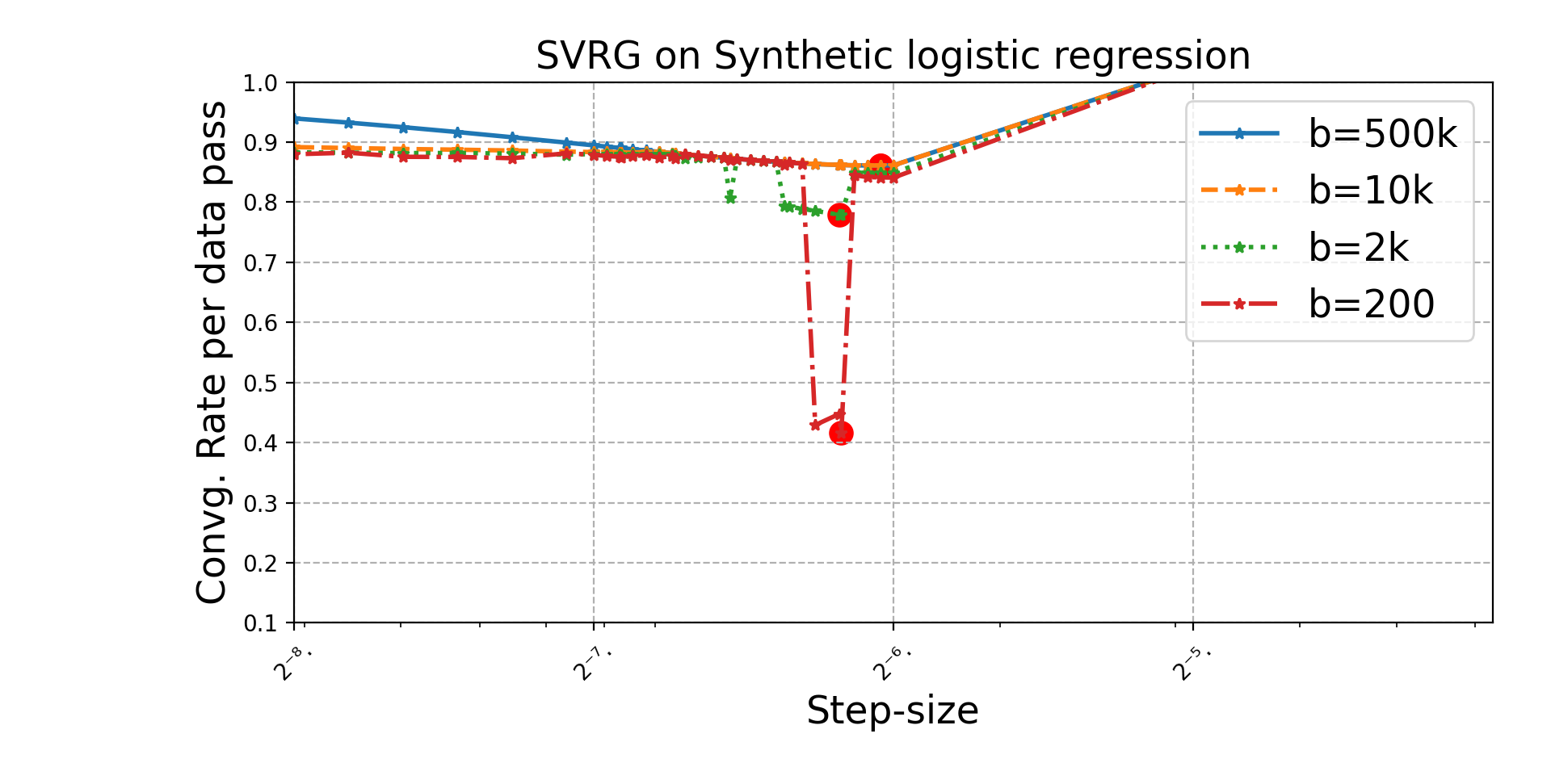
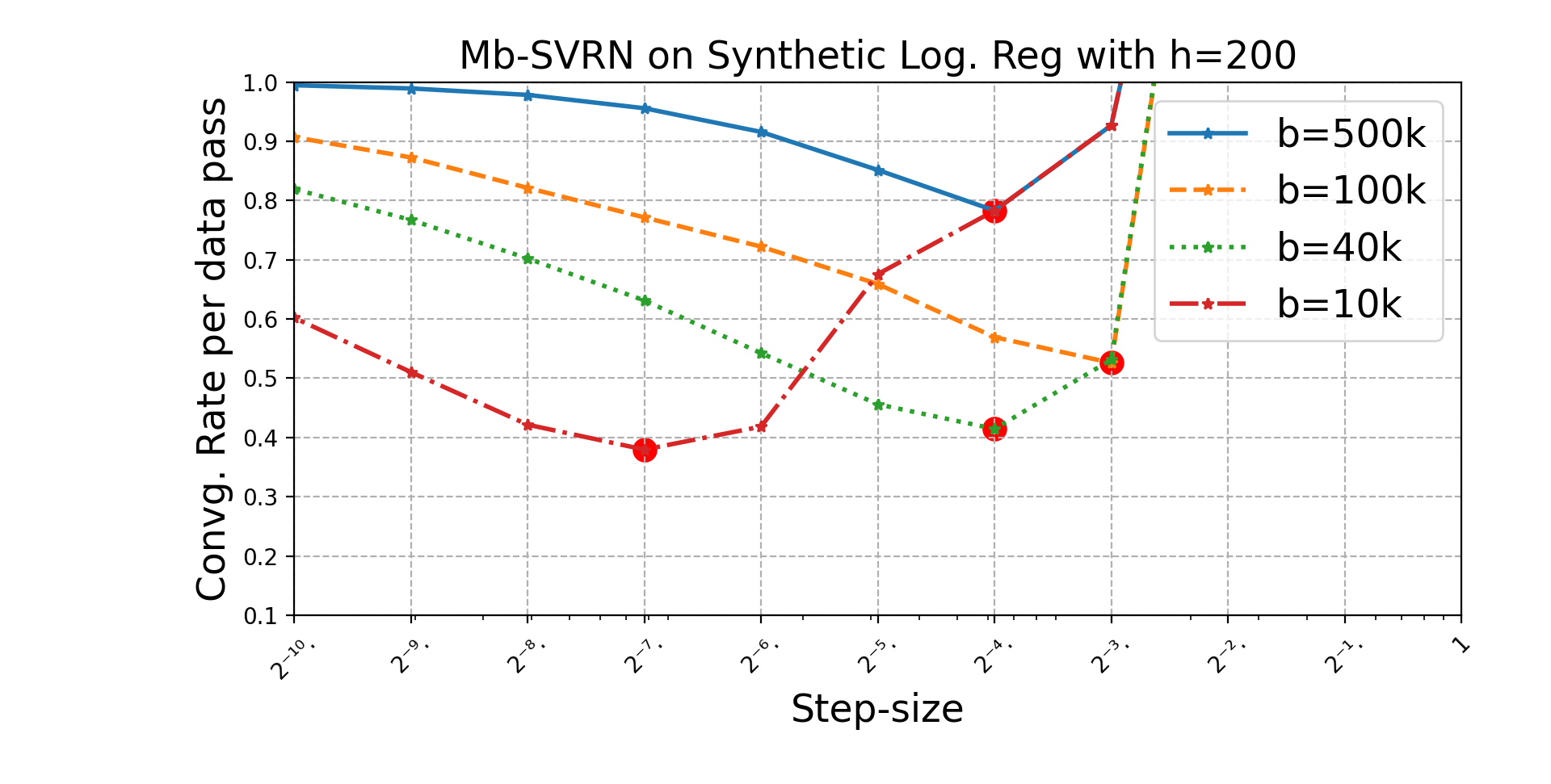
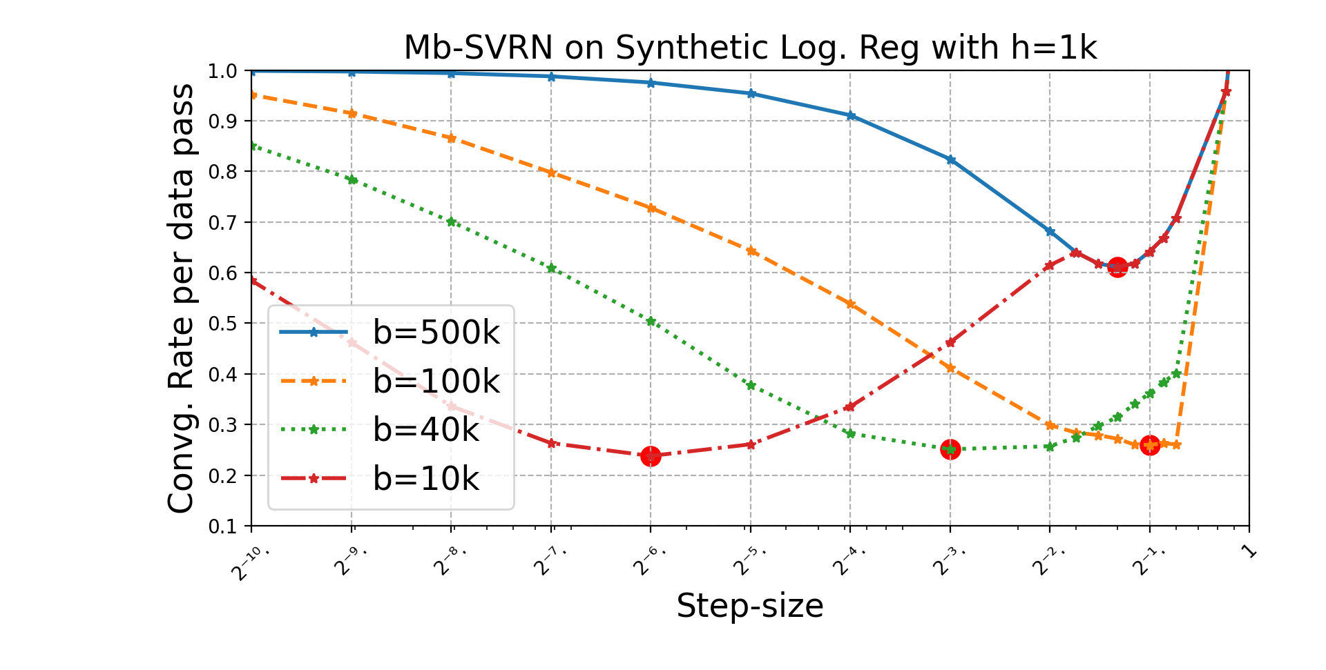
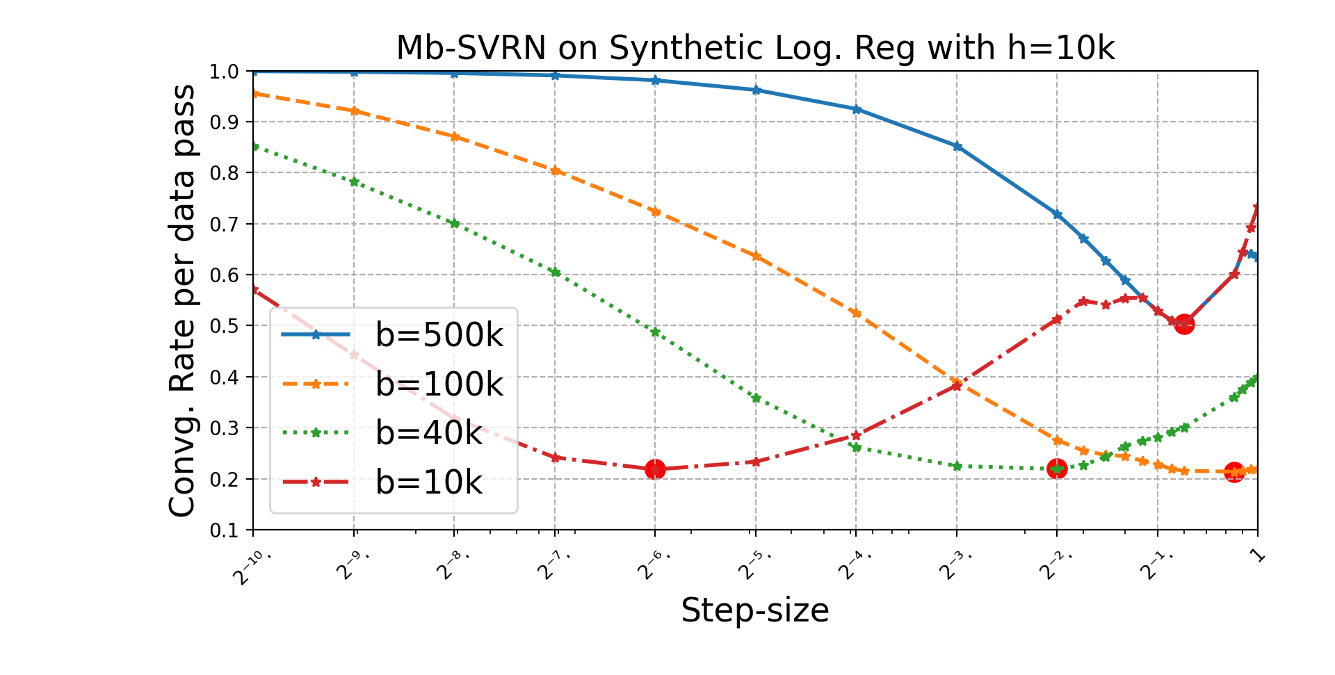
We first discuss Figure 4 showing the convergence rate of Mb-SVRN as we vary gradient mini-batch size and Hessian sample size for solving regularized logistic regression tasks on EMNIST and CIFAR10 datasets. The convergence rates reported are obtained after tuning the convergence rate per data pass with respect to the step size and number of inner iterations, for any value pair. The theory suggests that the convergence rate of Mb-SVRN is independent of the gradient mini-batch size for a wide range of mini-batch sizes, and the plot recovers this phenomenon remarkably accurately. The plot highlights that Mb-SVRN is robust to gradient mini-batch size, since the fast convergence rate of Mb-SVRN is preserved for a very large range of gradient mini-batch sizes (represented by the curves in Figure 4 staying flat). This can also be observed by noticing the almost straight line alignment of red marker dots in the Mb-SVRN plots in Figure 5. This phenomenon does not hold for first-order variance reduction methods. The plots demonstrate that the performance of SVRG suffers with increasing , which is consistent with the existing convergence analysis of SVRG-type first-order methods [15, 1].
We also note that as increases and enters into a very large gradient mini-batch size regime, the convergence rate of Mb-SVRN starts to deteriorate and effectively turns into Subsampled Newton (SN) when . The empirical evidence showing deterioration in convergence rate for very large values agrees with our theoretical prediction of a phase transition into standard Newton’s method after . In the extreme case of , Mb-SVRN performs only one inner iteration and is the same as SN. As SN uses the exact gradient at every iteration, its convergence rate per data pass is very sensitive to the Hessian approximation quality, which makes it substantially worse than Mb-SVRN for small-to-moderate Hessian sample sizes .
5.3 Robustness to step size
In addition to the demonstrated robustness to gradient mini-batch size, Mb-SVRN exhibits empirical resilience to step size variations. As depicted in Figure 5, the convergence rate for small values closely aligns with the optimal rate (red dot) when the step size approaches the optimal range. In contrast, the convergence rate of Subsampled Newton sharply increases near its optimal step size. This suggests that the convergence rate of Mb-SVRN with small-to-moderate gradient mini-batch size is more robust to changes in step size as compared to using very large gradient mini-batches or the full gradients. Intuitively, with smaller values, the algorithm performs numerous inner iterations, relying more on variance reduction. This advantage offsets the impact of step size changes. Conversely, with very large values, Mb-SVRN selects larger step sizes, reducing the number of optimal inner iterations and limiting the variance reduction advantage. On the other hand, for SVRG with very large gradient mini-batches, deviating slightly from the optimal step size can significantly impact the convergence rate per data pass, as seen with the sharp changes in convergence in the top two plots of Figure 5.
6 Conclusions and Future Directions
We have shown that incorporating second-order information into a stochastic variance-reduced method allows it to scale more effectively, and to scale to very large mini-batches. We have demonstrated this by analyzing the convergence of Mb-SVRN, a prototypical stochastic second-order method with variance reduction, and have shown that its associated convergence rate per data pass remains optimal for a very wide range of gradient mini-batch sizes (up to ). Our main theoretical result provides a convergence guarantee robust to the gradient mini-batch size with high probability through a novel martingale concentration argument. Furthermore, empirically we have shown the robustness of Mb-SVRN not only to mini-batch size, but also to the step size and the Hessian approximation quality. Our algorithm, analysis, and implementation uses SVRG-type variance reduced gradients, and as such, a natural question pertains to whether the algorithm can be extended to use other (perhaps biased) variance reduction techniques. Another interesting future direction is to investigate the effect of using alternate sampling methods while selecting component gradients, as well as the effect of incorporating acceleration into the method.
References
- [1] Allen-Zhu, Z.: Katyusha: The first direct acceleration of stochastic gradient methods. The Journal of Machine Learning Research 18(1), 8194–8244 (2017)
- [2] Allen-Zhu, Z.: Katyusha x: Practical momentum method for stochastic sum-of-nonconvex optimization. arXiv preprint arXiv:1802.03866 (2018)
- [3] Berahas, A.S., Bollapragada, R., Nocedal, J.: An investigation of newton-sketch and subsampled newton methods. Optimization Methods and Software 35(4), 661–680 (2020)
- [4] Berahas, A.S., Nocedal, J., Takác, M.: A multi-batch l-bfgs method for machine learning. Advances in Neural Information Processing Systems 29 (2016)
- [5] Berahas, A.S., Shi, J., Yi, Z., Zhou, B.: Accelerating stochastic sequential quadratic programming for equality constrained optimization using predictive variance reduction. Computational Optimization and Applications 86, 79––116 (2023)
- [6] Bollapragada, R., Byrd, R.H., Nocedal, J.: Exact and inexact subsampled newton methods for optimization. IMA Journal of Numerical Analysis 39(2), 545–578 (2019)
- [7] Bollapragada, R., Nocedal, J., Mudigere, D., Shi, H.J., Tang, P.T.P.: A progressive batching L-BFGS method for machine learning. In: International Conference on Machine Learning, pp. 620–629. PMLR (2018)
- [8] Bottou, L., Curtis, F.E., Nocedal, J.: Optimization methods for large-scale machine learning. SIAM review 60(2), 223–311 (2018)
- [9] Dereziński, M.: Stochastic variance-reduced newton: Accelerating finite-sum minimization with large batches. NeurIPS OPT 2023 Optimization in Machine Learning workshop (2023)
- [10] Derezinski, M., Mahajan, D., Keerthi, S.S., Vishwanathan, S., Weimer, M.: Batch-expansion training: an efficient optimization framework. In: International Conference on Artificial Intelligence and Statistics, pp. 736–744. PMLR (2018)
- [11] Erdogdu, M.A., Montanari, A.: Convergence rates of sub-sampled newton methods. Advances in Neural Information Processing Systems 28 (2015)
- [12] Gonen, A., Orabona, F., Shalev-Shwartz, S.: Solving ridge regression using sketched preconditioned svrg. In: International conference on machine learning, pp. 1397–1405. PMLR (2016)
- [13] Gower, R., Goldfarb, D., Richtárik, P.: Stochastic block bfgs: Squeezing more curvature out of data. In: International Conference on Machine Learning, pp. 1869–1878. PMLR (2016)
- [14] Johnson, R., Zhang, T.: Accelerating stochastic gradient descent using predictive variance reduction. Advances in neural information processing systems 26 (2013)
- [15] Konecnỳ, J., Richtárik, P.: Semi-stochastic gradient descent methods. arXiv preprint arXiv:1312.1666 (2013)
- [16] Lin, H., Mairal, J., Harchaoui, Z.: A universal catalyst for first-order optimization. Advances in neural information processing systems 28 (2015)
- [17] Liu, Y., Feng, F., Yin, W.: Acceleration of svrg and katyusha x by inexact preconditioning. In: International Conference on Machine Learning, pp. 4003–4012. PMLR (2019)
- [18] Lucchi, A., McWilliams, B., Hofmann, T.: A variance reduced stochastic newton method. arXiv preprint arXiv:1503.08316 (2015)
- [19] Minsker, S.: On some extensions of bernstein’s inequality for self-adjoint operators. arXiv preprint arXiv:1112.5448 (2011)
- [20] Mokhtari, A., Eisen, M., Ribeiro, A.: Iqn: An incremental quasi-newton method with local superlinear convergence rate. SIAM Journal on Optimization 28(2), 1670–1698 (2018)
- [21] Moritz, P., Nishihara, R., Jordan, M.: A linearly-convergent stochastic l-bfgs algorithm. In: Artificial Intelligence and Statistics, pp. 249–258. PMLR (2016)
- [22] Na, S., Dereziński, M., Mahoney, M.W.: Hessian averaging in stochastic newton methods achieves superlinear convergence. Mathematical Programming 201(1), 473–520 (2023)
- [23] Nesterov, Y., et al.: Lectures on convex optimization, vol. 137. Springer (2018)
- [24] Pilanci, M., Wainwright, M.J.: Newton sketch: A near linear-time optimization algorithm with linear-quadratic convergence. SIAM Journal on Optimization 27(1), 205–245 (2017)
- [25] Rigollet, P., Tong, X.: Neyman-pearson classification, convexity and stochastic constraints. Journal of Machine Learning Research (2011)
- [26] Robbins, H., Monro, S.: A stochastic approximation method. The annals of mathematical statistics pp. 400–407 (1951)
- [27] Roosta-Khorasani, F., Mahoney, M.W.: Sub-sampled newton methods. Mathematical Programming 174(1), 293–326 (2019)
- [28] Roux, N., Schmidt, M., Bach, F.: A stochastic gradient method with an exponential convergence rate for finite training sets. Advances in neural information processing systems 25 (2012)
- [29] Schmidt, M., Le Roux, N., Bach, F.: Minimizing finite sums with the stochastic average gradient. Mathematical Programming 162, 83–112 (2017)
- [30] Shalev-Shwartz, S., Zhang, T.: Stochastic dual coordinate ascent methods for regularized loss minimization. Journal of Machine Learning Research 14(1) (2013)
- [31] Sharpe, W.F.: Mean-variance analysis in portfolio choice and capital markets (1989)
- [32] Tropp, J.: Freedman’s inequality for matrix martingales. Electronic Communications in Probability 16, 262–270 (2011)
- [33] Tropp, J.A.: User-friendly tail bounds for sums of random matrices. Foundations of computational mathematics 12, 389–434 (2012)
- [34] Xiao, L., Zhang, T.: A proximal stochastic gradient method with progressive variance reduction. SIAM Journal on Optimization 24(4), 2057–2075 (2014)
Appendix A Proofs
A.1 Proof of Lemma 1.
Proof As each is convex and -smooth, the following relation holds (see Theorem 2.1.5 in [23]),
Consider the variance of the stochastic gradient if we use just one sample, for calculating the stochastic gradient. The variance is given as .
| (24) |
Similarly, if we use samples and upper bound ,
Now as all the indices are chosen independently, we can write the variance of the sum as the sum of individual variances.
| (25) |
where in the last inequality, we used (24). Since has continuous first and second-order derivatives, we can use the quadratic Taylor’s expansion for around . For vectors and , such that,
Let , , we get,
Using the assumption , we have . Take , we have ,
implying,
Substitute the above relation in (25), we get,
A.2 Proof of Lemma 2.
Proof For the sake of this proof we abuse the notation and write as . However we make clear that Mb-SVRN uses . In this proof we denote , , and .
where . We upper bound as,
As , for any , we have , and therefore . Also we have and . Combining these positive semidefinite orderings for and along with , we have . We get,
implying that,
Since , and , maximum value would be . We get,
and hence,
Changing to we get,
Using , we conclude,
A.3 Proof of Lemma 3.
In the proof, we will use a result from [19], stated as the following,
Lemma 12 (Matrix Bernstein: Corollary 4.1 from [19])
Let be a sequence of random vectors such that , almost surely . Denote . Then ,
We now return to the proof of Lemma 3.
Proof Define random vectors , as . Then . Also,
We also have the following upper bound on the variance of :
Since is twice continuously differentiable, there exists a such that,
Using the assumption that , with we have . With , and ,
We get,
So we take and . Also note that, . Look for such that,
Now in the regime of we have . Consider , . For this value of , we get with probability ,
This means with probability ,
Moreover, in the regime of , we have . In this case set . We conclude,
A.4 Proof of Lemma 4.
Proof Since , we have . Consider the following,
Denoting , we get,
Since we have and , we have . Furthermore for , we have , because for all . So we use the results and and get,
A.5 Proof of Theorem 3.
In our proof of Theorem 3, we use a Master tail bound for adapted sequenced from [32]. Let be a filtration and random process be measurable. Also let another random process such that is measurable. Consider the difference sequence for ,
Also, assume the following relation holds for a function :
Then we have,
Theorem 7 (Master tail bound for adapted sequences [32])
For all , we have,
In our proof, we also use the following Lemma from [32]. The original version of the result assumes that , however, we show below that the proof also holds for the case when .
Lemma 13 (Freedman MGF, Lemma 6.7 from [33])
Let be a random variable such that and almost surely. Then for any and ,
Proof Consider the Taylor series expansion of ,
Replace with the random variable and take expectation on both sides, we get,
On the second term use and on the third term use to get almost surely, we get,
We now return to the proof of Theorem 3.
Proof If is a submartingale we have,
and also we know that . For , consider . Clearly, is measurable. We now establish the relation that . For any , consider a function defined as follows,
It is easy to show that is an increasing function of . Using Lemma 13 we get for . Now we can use the Master tail bound Theorem 7. The only thing remaining to analyze is,
Doing little calculus shows that, minimizes and the minimum value is . Finally observe that . This completes the proof.
A.6 Proof of Theorem 6.
Proof Using the -smoothness of , we know that
Substitute , we get,
Take total expectation on both sides, by which we mean expectation conditioned only on known . We get,
Here in the last inequality, means conditional expectation, conditioned on known . Analyzing the inner expectation , we get,
where we obtained that second term due to the unbiasedness of stochastic gradient i.e., . Furthermore using unbiasedness we have . We get,
Since , where we used to write . Substituting we get,
Again using , we get . Also note that and hence . We get,
Now use . Also due to -strong convexity of we have . We get,
Subtract from both sides we get,
| (26) |
We denote . Since we perform inner iterations before updating , we recursively unfold the relation (26) for times. This provides the following,
For , we have . Substituting upper bound for we get,
Let , we get,
Now if we get,
otherwise if , then we consider two cases based on the value of . If then we get,
and if then,
This completes the proof.
Appendix B Additional Plots for Synthetic Data Experiments
For designing synthetic data, we considered two random orthonormal matrices and and constructed a matrix where is a diagonal matrix with large condition number . In , we set diagonal entries to be and only one diagonal entry as , artificially enforcing a very large condition number. For constructing labels, we set where is the row of and is a random vector drawn from an isotropic multivariate Gaussian distribution. Also, we fix the regularization parameter to .
Our empirical results for the synthetic data are presented in Figure 6. In plot 6a, we observe the sensitivity of the peformance of SVRG to the gradient mini-batch size, and step size. Unlike SVRG, we empirically observe the robustness of Mb-SVRN to gradient mini-batch size. This is demonstrated clearly in our plots by an almost flat-line alignment of red dots for and . Note that the optimal step size for SVRG is close to for all gradient mini-batch sizes, and the slight deviation from this optimal step size leads to rapid deterioration in the convergence rate. On the other hand, in Figures 6b-6d, we see the convergence rate curves for different gradient mini-batch sizes exhibit a flatter behavior near their respective optimal step sizes, demonstrating the robustness of Mb-SVRN to the step size. In addition to robustness, the plots also demonstrate the faster overall convergence rate of Mb-SVRN.
