FusionPortableV2: A Unified Multi-Sensor Dataset for Generalized SLAM Across Diverse Platforms and Scalable Environments

Abstract

Simultaneous Localization and Mapping (SLAM) technology has been widely applied in various robotic scenarios, from rescue operations to autonomous driving. However, the generalization of SLAM algorithms remains a significant challenge, as current datasets often lack scalability in terms of platforms and environments. To address this limitation, we present FusionPortableV2, a multi-sensor SLAM dataset featuring notable sensor diversity, varied motion patterns, and a wide range of environmental scenarios. Our dataset comprises $27$ sequences, spanning over $2.5$ hours and collected from four distinct platforms: a handheld suite, wheeled and legged robots, and vehicles. These sequences cover diverse settings, including buildings, campuses, and urban areas, with a total length of $38.7km$. Additionally, the dataset includes ground-truth (GT) trajectories and RGB point cloud maps covering approximately $0.3km^{2}$. To validate the utility of our dataset in advancing SLAM research, we assess several state-of-the-art (SOTA) SLAM algorithms. Furthermore, we demonstrate the dataset’s broad applicability beyond traditional SLAM tasks by investigating its potential for monocular depth estimation. The complete dataset, including sensor data, GT, and calibration details, is accessible at https://fusionportable.github.io/dataset/fusionportable_v2.

1 Introduction

1.1 Motivation

Real-world robotics datasets play a crucial role in the development of SLAM. They not only cover a wide range of environments but also feature intricately designed sequences that pose challenges. They serve as essential resources for thoroughly training and evaluating SLAM systems and circumventing the reliance on complex and potentially imprecise physical simulations. Moreover, such datasets eliminate the need for budget and workforce, such as system integration, calibration, and extensive field operations (Nguyen et al., 2022). These accessible resources allow for broader participation in SLAM research, facilitating development of novel algorithms without relying on high costs or specialized expertise. Currently, datasets become particularly important since the field of robotics research is experiencing a paradigm shift from traditional handcrafted and model-based methodologies to data-driven approaches (Brohan et al., 2022; Shah et al., 2023b), alongside the emergence of hybrid strategies.

The robustness and performance of large-scale and long-term SLAM strongly rely on a robot’s perceptual capability, especially in field environments (e.g., subterranean (Reinke et al., 2022) and forest (Knights et al., 2023)). As outlined in Table 1, SLAM datasets, encompassing a wide range of scenarios from both simulated and real-world environments, are increasingly being augmented with multi-modal sensor data, moving beyond the traditional reliance on singular modal inputs like images. For example, cameras capture dense and high-resolution 2D images containing texture and pattern information of surroundings. However, cameras are vulnerable to adverse illumination conditions (e.g., darkness and glare) due to their passive nature in measuring. In contrast, range sensors such as LiDARs and Radars provide sparse but highly accurate structural information by exploiting their respective light sources. Integrating cameras with range sensors often yields more reliable results across a variety of perception tasks compared to relying on a single sensor type (Lai et al., 2022). Therefore, the complementary strengthes offered by various sensors drives the exploration of novel sensor fusion algorithms (Lin and Zhang, 2022), enabling robots to autonomously navigate through diverse environments with increased accuracy and robustness.

Despite the advancements in SLAM, there remains a notable deficiency in the diversity and breadth of available SLAM datasets, especially concerning variations in environments, sensor modalities, and platforms executing diverse motions. This limitation affects the algorithms’ flexibility and applicability in real-world scenarios, underlining an immediate need for more inclusive datasets. Drawing on the recent success in training generalized manipulation (Brohan et al., 2022) and navigation (Shah et al., 2023a) models, it is our conviction that datasets featuring high motion and environmental diversity are crucial for the development of a versatile, generalized SLAM system.

1.2 Contributions

Following this route, this paper aims to introduce a comprehensive multi-sensor dataset with a standardized format, share insights and methodologies from our data collection process, and provide benchmarking tools along with GT for evaluating various algorithms. Building upon our previous open-source FusionPortable dataset (Jiao et al., 2022), we present FusionPortableV2, an extensive upgrade that broadens the dataset in terms of data modalities, scenarios, and motion capabilities. The key contributions of this paper are threefold:

1. We introduce significant improvements to the FusionPortable dataset by extending the spectrum of platforms to encompass high-speed vehicles and spanning more than $12$ types of environments (e.g., campuses, underground areas, parking lots, highways, etc.). These enhancements not only enrich the dataset’s diversity and complexity but also bring substantial upgrades in the precision of ground truth data and the integration of raw kinematic data collected from ground robots. Our collection encompasses $27$ sequences, spanning $2.5$ hours and covering a total distance of $38.7km$.

2. We furnish detailed ground truth trajectories and maps, encompassing an area of around $0.3km^{2}$, for most of the sequences. This facilitates a more thorough algorithm evaluation and supports a wide range of research objectives. The rich variety of platforms and settings in our dataset exemplifies its utility as a benchmark for assessing various navigation algorithms beyond SLAM.

3. We have expanded the utility of the dataset by incorporating experiments on monocular depth estimation, addressing both the training and evaluation stages, in addition to localization and mapping. Throughout the process of platform development and data collection, we have tackled numerous technical challenges and have meticulously described the encountered issues and their solutions. This guidance is intended to serve as a valuable resource for future researchers in the field. To foster collaborative advancements, we have publicly released all data and implementation details, aiming to open up extensive research avenues in field robotics and contribute to the development of versatile and resilient robotic systems.

1.3 Organization

The remainder of this paper is structured in the following manner: Section 2 discusses related works most of on SLAM datasets and summarizes key contributions of this paper. Section 3 outlines the hardware setup and sensor details. Section 4 covers sensor calibration procedures. Section 5 describes the dataset, including platform characteristics and scenarios. Section 6 introduces details post-processing steps on raw sensor measurements and GT data. Section 7 presents the methodologies used for evaluating localization, mapping, and mocular depth estimation. Known issues of this dataset are also dicussed. Finally, Section 8 concludes the paper and suggests directions for future research.

2 Related Works

Table 1: Comparing SLAM Datasets: Highlights differences in platforms, sensors, and ground-truth methods, focusing on FusionPortableV2’s attributes. It classifies environment scales into small ($<100m^{2}$), medium ($<500m^{2}$), and large, acknowledging this as a broad estimation. Abbreviations include: UGV (Unmanned ground vehicle), MoCap (Motion capture), LT (Laser tracker), O (Out-of-the-box kinematic-inertial odometry),S (subterranean), and V (vegetated) areas. The symbol ● and ○ indicate whether dataset satisfies the option or not. ◑ indicates that the dataset misses robot kinematic data.

Dataset	Sensors Modality					Mobile Platform				Environment Scale			GT Pose	GT Map
	IMU	Frame Camera	Event Camera	LiDAR	GPS	Handhold	UGV	Legged	Vehicle	Small	Medium	Large
UZH-Event (Mueggler et al., 2017)	●	○	●	○	○	●	○	○	○	●	●	○	MoCap
PennCOSYVIO (Pfrommer et al., 2017)	●	●	○	○	○	●	○	○	○	●	●	○	Apriltag
TUM VI (Schubert et al., 2018)	●	●	○	○	○	●	○	○	○	●	●	●	MoCap
UMA-VI (Zuñiga-Noël et al., 2020)	●	●	○	○	○	●	○	○	○	●	●	●	SfM
Newer College (Ramezani et al., 2020)	●	●	○	●	○	●	○	○	○	●	●	○	ICP	Scanner
Hilti-Oxford (Zhang et al., 2022)	●	●	○	●	○	●	○	○	○	●	○	○	ICP	Scanner
VECTor (Gao et al., 2022)	●	●	●	●	○	●	○	○	○	●	○	○	MoCap/ ICP	Scanner
MIT DARPA (Huang et al., 2010)	●	●	○	●	●	○	○	○	●	○	○	●	D-GNSS
KITTI (Geiger et al., 2013)	●	●	○	●	●	○	○	○	●	○	○	●	RTK-GNSS
Oxford RobotCar (Maddern et al., 2017)	●	●	○	●	●	○	○	○	●	○	○	●	D-GNSS
KAIST-Complex Urban (Jeong et al., 2019)	●	●	○	●	●	○	○	○	●	○	○	●	RTK-GNSS	SLAM
Ford Multi-AV (Agarwal et al., 2020)	●	●	○	●	●	○	○	○	●	○	○	●	D-GNSS	SLAM
DSEC (Gehrig et al., 2021)	○	●	●	●	●	○	○	○	●	○	○	●	RTK-GNSS	SLAM
Boreas (Burnett et al., 2023)	●	●	○	●	●	○	○	○	●	○	○	●	RTX-GNSS
NCLT (Carlevaris-Bianco et al., 2016)	●	●	○	●	●	○	●	○	○	●	●	○	RTK-GNSS/ SLAM
MVSEC (Zhu et al., 2018)	●	●	●	●	●	●	○	○	●	●	○	●	GNSS/ MoCap/ SLAM	SLAM
Rosario (Pire et al., 2019)	●	●	○	○	●	○	●	○	○	○	●(V)	○	RTK-GNSS
M2DGR (Yin et al., 2021)	●	●	●	●	●	○	◑	○	○	●	●	○	RTK-GNSS/ MoCap/ LT
Nebula (Reinke et al., 2022)	●	○	○	●	●	○	●	◑(O)	○	○	●(S)	○	SLAM	Scanner
FusionPortable (Jiao et al., 2022)	●	●	●	●	●	●	◑	◑	○	●	●	○	MoCap/ RTK-GNSS/ NDT	Scanner
M3ED (Chaney et al., 2023)	●	●	●	●	●	○	○	◑	●	●	●(V)	●	RTK-GNSS/ SLAM	SLAM
Ours (FusionPortableV2)	●	●	●	●	●	●	●	●	●	●	●	●	RTK-GNSS/ LT	Scanner

In the last decade, high-quality datasets have crucially driven SLAM algorithm advancements, yielding significant time and cost savings in platform development and data acquisition. The rapid progress in sensor and robotics technology has led to the widespread adoption of multi-modal sensors across various robotic platforms, as detailed in Table 1. This evolution has set new benchmarks and hastened the enhancement of SOTA algorithms, covering both handcrafted and data-driven methods like VINS-Mono (Qin et al., 2018), FAST-LIO2 (Xu et al., 2022), VILENS (Wisth et al., 2022), DROID-SLAM (Teed and Deng, 2021), and Gaussian Splatting SLAM (Matsuki et al., 2023).

2.1 Specific Platform Datasets

A wide array of SLAM datasets predominantly highlights visual-inertial fusion, targeting specific mobile platforms and venues. Platfors are ranged from handheld devices (Pfrommer et al., 2017; Schubert et al., 2018; Zuñiga-Noël et al., 2020) to drones (Burri et al., 2016; Majdik et al., 2017), unmanned ground vehicles (Pire et al., 2019), and aquatic vehicles such as canoes (Miller et al., 2018). Among them, the UZH-FPV dataset (Delmerico et al., 2019) is featured by its extended, rapid trajectories from aggressive drone flight with the integration of event cameras.

Urban environment datasets introduce specific challenges like adverse lighting, weather conditions, and larger scales. Long-range sensors, notably LiDARs and Radars, are preferred for their capabilities. The KITTI dataset (Geiger et al., 2013) sets a benchmark in autonomous driving with its rich urban sensor data collection, including LiDAR and cameras. Further developments in driving datasets have expanded across dimensions of duration (Maddern et al., 2017), urban complexity (Jeong et al., 2019), and weather adversity (Agarwal et al., 2020). The DSEC dataset (Gehrig et al., 2021), akin to UZH-FPV, leverages stereo event cameras for extensive driving scenes. Moreover, Radars are essential for outdoor perception, offering advantages in range, velocity measurement via the Doppler effect, and weather resilience. Radar-focused datasets like Boreas (Burnett et al., 2023), Oxford Radar Robocar (Barnes et al., 2020), and OORD (Gadd et al., 2024) collected data in conditions such as fog, rain, and snow.

Campus-scene datasets such as NCLT (Carlevaris-Bianco et al., 2016), M2DGR (Yin et al., 2021), NTU-Viral (Nguyen et al., 2022), ALITA (Yin et al., 2022), and FusionPortable (Jiao et al., 2022) also pose challenges for SLAM, given their diverse environmental appearance and structure. A typical campus features a variety of environments, inculding dense vegetation, open spaces, and complex buildings with multiple levels and detailed layouts. The changing lighting, seasonal foliage variations, and movement of pedestrians and vehicles add complexity to campus environments. The NCLT dataset highlights these factors as crucial for life-long SLAM challenges. However, despite their value, these datasets, collected via specific platforms like unmanned ground vehicles (UGVs) and drones, fall short in showcasing diverse motion patterns, especially aggressive maneuvers.

The Newer College dataset (Ramezani et al., 2020), Hilti-Oxford Dataset (Zhang et al., 2022), and MARS-LVIG dataset (Li et al., 2024) demonstrated the portable multi-sensor suites for collecting multi-modal data in a wide range of environments. Driven by the evaluation need for reconstruction and $6$-DoF motion estimates, the former two datasets additionally provide dense 3D global maps and allow the evaluation of mapping performance.

2.2 Multiple Platforms Datasets

Recent SLAM research trends emphasize algorithm generalization across different platforms and scales, aiming for motion characteristic integration from varied platforms with minimal parameter tuning for diverse scenarios. The MVSEC dataset (Zhu et al., 2018) pioneered in capturing multi-sensor data across platforms, excluding UGV sequences. Conversely, the Nebula dataset (Reinke et al., 2022), developed during the DARPA Subterranean Challenge, includes field environments with wheeled and legged robots, offering precise maps and trajectories but missing urban data and having varied sensor setups across platforms. The M3ED dataset (Chaney et al., 2023), although closely aligned with our objectives, lacks indoor data and platform-specific kinematic measurements, underscoring the unique contribution of our dataset.

Table 2: The sensors used in this dataset and their corresponding specifications

Sensor	Characteristics	ROS Topic	ROS Message Type	Rate (Hz)
3D LiDAR	Ouster OS$1$-$128$, $45^{\circ}$vert.$\times$ $360^{\circ}$horiz. FOV	/os_cloud_node/points	sensor_msgs/PointCloud2	$10$
	IMU: ICM$20948$, $9$-axis MEMS	/os_cloud_node/imu	sensor_msgs/Imu	$100$
	Range, near-ir, reflectivity, signal images	/os_image_node/(range,nearir,...)_image	sensor_msgs/Image	$10$
Frame Camera	Stereo FILR BFS-U$3$-$31$S$4$C, global shutter $66.5^{\circ}$vert. $\times$ $82.9^{\circ}$horiz. FOV $1024\times 768$ resolution	/stereo/frame_(left,right)/image_raw	sensor_msgs/CompressedImage	$20$
Event Camera	Stereo DAVIS$346$, $67^{\circ}$vert., $\times$ $83^{\circ}$horiz. FOV $346\times 240$ resolution	/stereo/davis_(left,right)/events	dvs_msgs/EventArray	$30$
	Images that capture color data	/stereo/davis_(left,right)/image_raw	sensor_msgs/CompressedImage	$20$
	IMU: MPU$6150$, $6$-axis MEMS	/stereo/davis_(left,right)/imu	sensor_msgs/Imu	$1000$
IMU	STIM$300$, $6$-axis MEMS	/stim300/imu	sensor_msgs/Imu	$200$
INS	$3$DM-GQ$7$-GNSS/INS Dual-antenna, RTK-enabled INS	/3dm_ins/nav/odom	nav_msgs/Odometry	$10$
		/3dm_ins/gnss_(left,right)/fix	sensor_msgs/NavStatFix	$10$
		/3dm_ins/imu	sensor_msgs/Imu	$200$
Wheel Encoder	Omron E6B2-CWZ6C, $1000$P/R	/mini_hercules/encoder	sensor_msgs/Joinstate	$100$
Legged Sensor	Built-in joint encoders and contact sensors	/unitree/joint_state	sensor_msgs/JointState	$50$
	Built-in IMU	/unitree/imu	sensor_msgs/Imu	$50$
	Out-of-the-box kinematic-ineratial odometry	/unitree/body_odom	nav_msgs/Odometry	$50$

2.3 Robot-Agnostic General Models

Recent progress in natural language processing and visual perception has spurred research into universal, robot-agnostic models for zero-shot transfer or task-specific fine-tuning, highlighting the need for expansive datasets. The Open X-Embodiment dataset (Padalkar et al., 2023) demonstrates this by presenting over $500$ skills across $22$ robot types, emphasizing the crucial role of large-scale datasets in robotic manipulation advancement. The DROID dataset (Khazatsky et al., 2024), collected by 13 institutions using identical hardware configurations to maximize portability and flexibility, further contributing to the advancement of robotic manipulation research. Likewise, the General Navigation Model (GNM) (Shah et al., 2023a) underlines the value of flexible, scalable navigation methods. Trained on diverse robot datasets, GNM’s unified model excels in various settings, even with sensor and actuator issues. Our objective aligns with that of GNM, with a specific focus on datasets: we aim to offer diverse, high-quality data towards the development and benchmark of more generalized and more robust SLAM algorithms.

3 System Overview

Figure 1: CAD model of the sensor rig where axes are marked: red: $X$, green: $Y$, blue: $Z$. It visualizes the position of each component of the handheld multi-senosr suite.

Figure 2: Data collection framework, highlighting the data flow and synchronization processes. The Red arrow indicate PPS signals for synchronization, green arrows show UTC time synchronization, and blue arrows represent sensor triggering signals, and black arrows depict the flow of raw data.

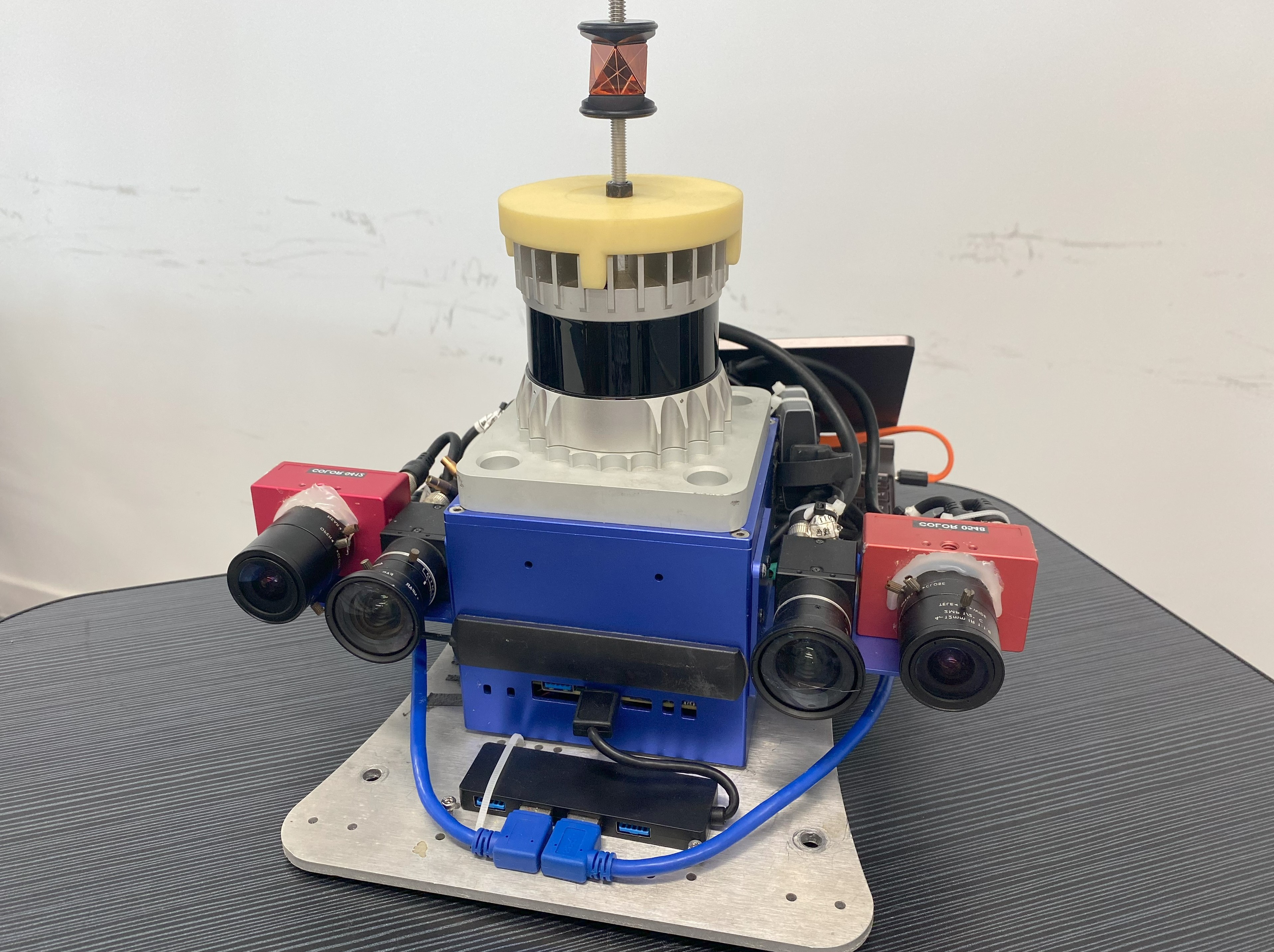
This section presents our developed multi-sensor suite, designed for easy integration with various mobile platforms through plug-and-play functionality. All sensors are securely mounted on a precision-engineered aluminum alloy frame, facilitating a unified installation. Additionally, we detail the devices employed for collecting GT trajectories and maps.

3.1 Suite Setup and Synchronization

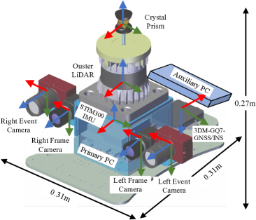
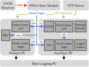
The Multi-Sensor Suite (MSS) integrates exteroceptive and proprioceptive sensors, including a 3D Ouster LiDAR, stereo frame and event cameras, and IMUs, depicted in its CAD model in Fig. 1. To manage data collection efficiently, we use two PCs synchronized via the Network Time Protocol (NTP) server. The primary PC processes data from the frame cameras and IMU, while the auxiliary PC handles additional data types. Both PCs are equipped with a $1$TB SSD, $64$GB of DDR4 memory, and an Intel i$7$ processor, running Ubuntu with a real-time kernel patch and employing the Robot Operating System (ROS) for data collection. Subsequent sections will elaborate on our data synchronization approach and the specific features of each sensor.

(a) Top View of the UGV.

(b) Side View of the UGV.

(c) Legged Robot.

(d) High-Speed Vehicle.

Figure 3: Layouts of the platform-specific sensor setup, including different coordinate systems and their relative translation.

3.1.1 Synchronization:

The synchronization process is illustrated in Fig. 2. The FPGA board synchronizes with the pulse-per-second (PPS) signal from its internal GNSS module, producing frequency trigger signals for the IMU, stereo frame cameras, and LiDAR clock alignment. In GPS-denied environments, it utilizes its internal low drift oscillator for synchronization, achieving a time accuracy below $1ms$ for multisensor data collection. For better integration of LiDAR and camera data, we directly synchronize the LiDAR’s phase with the camera’s capture timing. The event cameras, having their own synchronization mechanism, are connected through a designated port. The left event camera, assigned as the master, sends trigger signals to the right camera.

3.1.2 Inertial Measurement Unit:

The STIM$300$ IMU, a tactical-grade sensor, forms the primary inertial sensor of our system, mounted beneath the LiDAR. Its bias instability for the gyroscope and accelerometer is $0.3^{\circ}/h$ and $0.04mg$, respectively. outputs angular velocity and acceleration measurements at $200Hz$. Other components, including the LiDAR, event cameras, and the $3$DM-GQ$7$ INS, also integrate IMUs. Further details are provided in subsequent sections.

3.1.3 3D LiDAR:

Our LiDAR choose the OS1-$128$ Gen$5$ LiDAR that operates at $10Hz$. It features a built-in IMU capturing gyroscope, acceleration, and magnetometer data and generates four types of images to facilitate the usage of image-based algorithms: range, near-ir, reflectivity, and signal image. Each image measures different properties of the surroundings: (1) range images display the distance of the point from the sensor origin, calculated using the time of flight of the laser pulse; (2) near-ir images capture the strength of sunlight at the $865nm$ light wavelength collected, also expressed in the number of photons detected that was not produced by the sensor’s laser pulse; (3) reflectivity images display the reflectivity of the surface or object that was detected by the sensor; and (4) signal images show the strength of the light returned from the given point, which is influenced by various factors including distance, atmospheric conditions, and objects’ reflectivity.

3.1.4 Stereo Frame Cameras:

Our setup includes two FLIR BFS-U$3$-$31$S$4$C global-shutter color cameras for stereo imaging, synchronizing to output images at $1024\times 768$ pixels and $20Hz$. The exposure time $\tau$ for both cameras is manually set as a fixed value. Image timestamps are adjusted by subtracting $0.5\tau$ to approximate the true trigger time. To prevent abrupt changes in color space, the white balance settings are also fixed. Additionally, metadata like exposure time and gain are included for detailed image analysis.

3.1.5 Stereo Event Cameras:

The system includes two event cameras known for their high temporal resolution, extensive dynamic range, and energy efficiency. With a $346\times 260$ pixel resolution, these cameras come with an internal IMU for high-rate data output. Frame images cannot be synchronized, resulting in $10$-$20ms$ delay. Infrared filters are used to lessen LiDAR light interference. Exposure times are set fixedly, whereas outdoor settings use auto-exposure to maintain image quality under varying light conditions.

3.2 Platform-Specific Sensor Setup

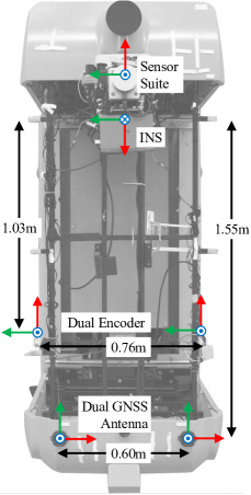
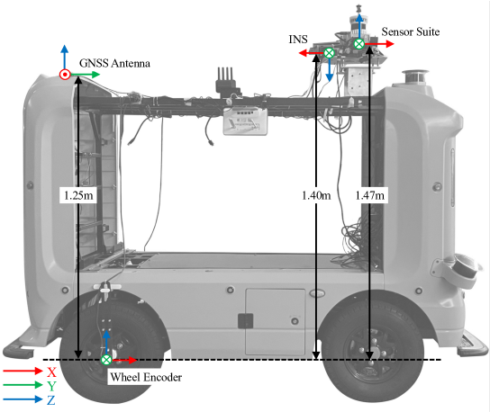
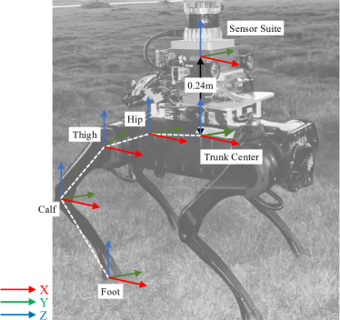
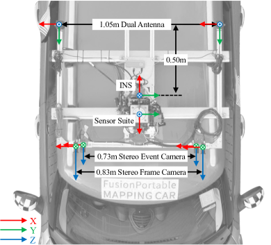
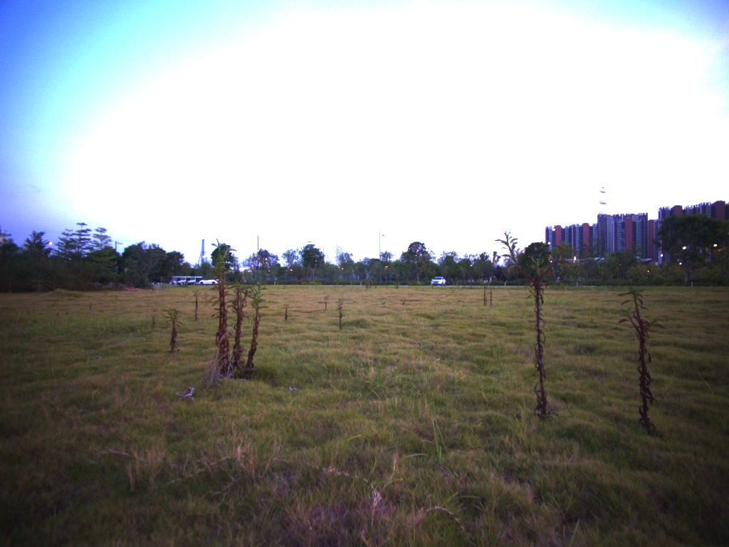
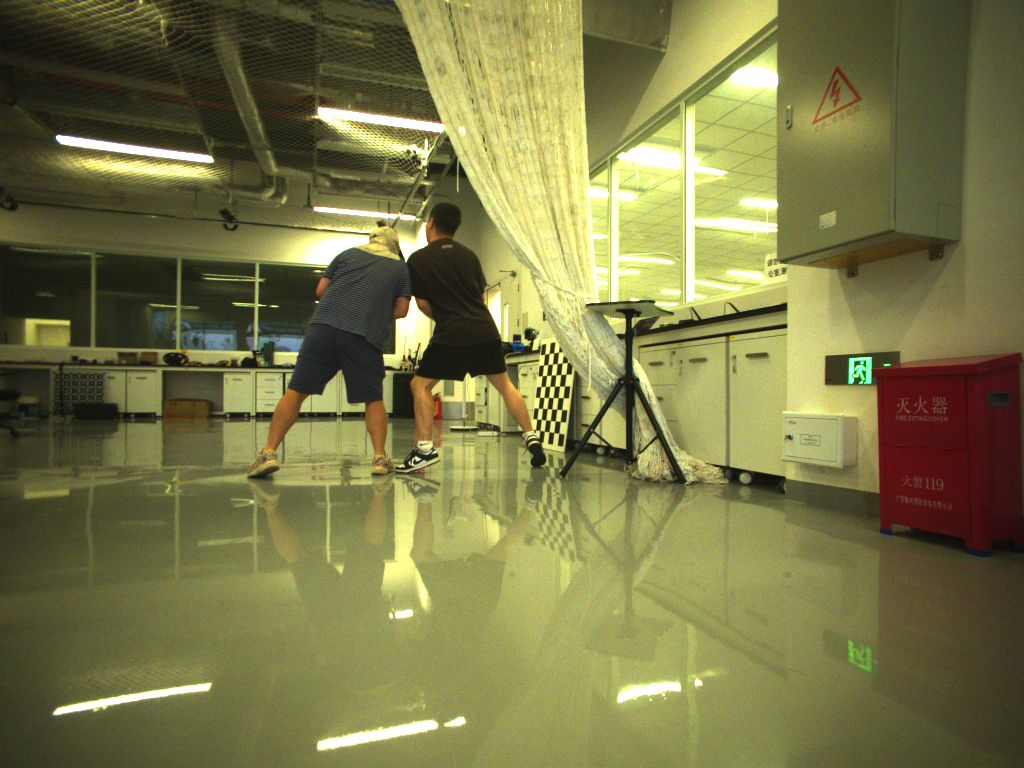
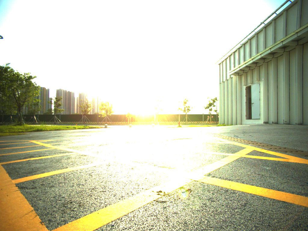
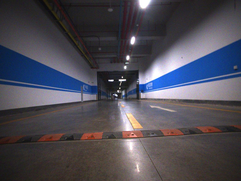
Our goal is to create a diverse dataset by capturing sequences with multiple mobile platforms, thereby increasing the dataset’s complexity and challenge compared to those relying on a single platform. Each platform is equipped with a handheld multi-sensor suite and platform-specific sensors, as shown in Fig. 3. Fig. 4 displays the platforms and exemplifies typical scenes from which data were gathered. Platform-specific sensor settings are introduced in the subsequent sections, while the description of their motion and scenario patterns are presented in Section 5.1.

3.2.1 Legged Robot:

We have selected the Unitree A1 quadruped robot as our legged platform, as shown in Fig. 3(c) This robot is equipped with $12$ joint motor encoders and $4$ contact sensors per leg, located at the hip, thigh, calf, and foot. These sensors provide kinematic measurements at a rate of $50Hz$. The MSS is affixed to the robot’s dorsal side and communicates with the kinematic sensors via Ethernet. In addition to the raw sensor measurements, we record metadata for each motor, which includes torque, velocity, position, and temperature, along with kinematic-inertial odometry data.

3.2.2 Unmanned Ground Vehicle:

The MSS is integrated into a four-wheeled Ackerman UGV (see Fig. 3(a), 3(b)), originally designed for logistics transportation (Liu et al., 2021). To optimize signal reception, the dual GNSS antennas of the $3$DM-GQ$7$ are positioned at UGV’s rear side. Kinematic data for the UGV is acquired through two incremental rotary encoders, strategically positioned at the center of the rear wheel. These encoders, featuring $1000$ pulses per revolution, produce measurement data at a rate of approximately $100Hz$, which is then recorded.

3.2.3 Vehicle:

As depicted in Fig. 3(d), we follow the KITTI setup (Geiger et al., 2013) by extending the baseline of both the stereo cameras and the dual antenna, with the stereo frame camera having a baseline of $83cm$ and the event camera having a baseline of $73cm$. This extended baseline enhances the accuracy of depth estimation for distant objects, as compared with that in the UGV. The MSS is securely mounted on the vehicle’s luggage rack using a custom-designed aluminum frame.

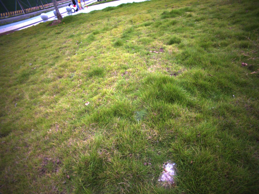
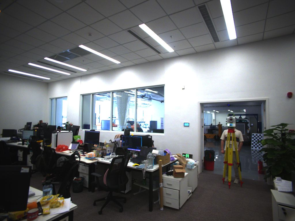
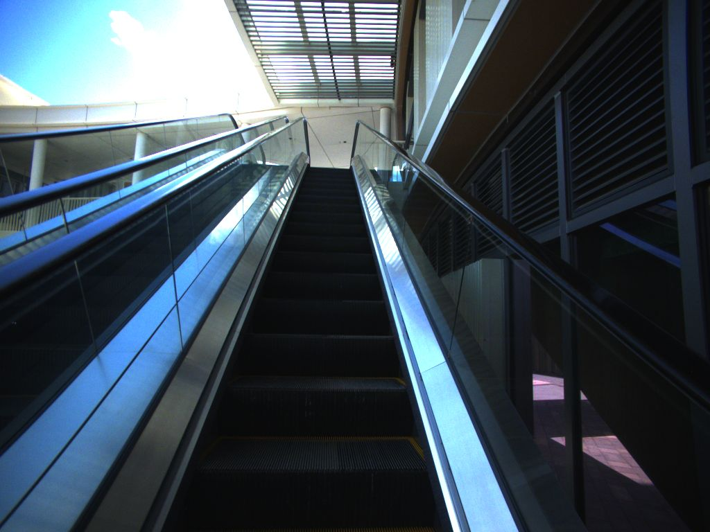
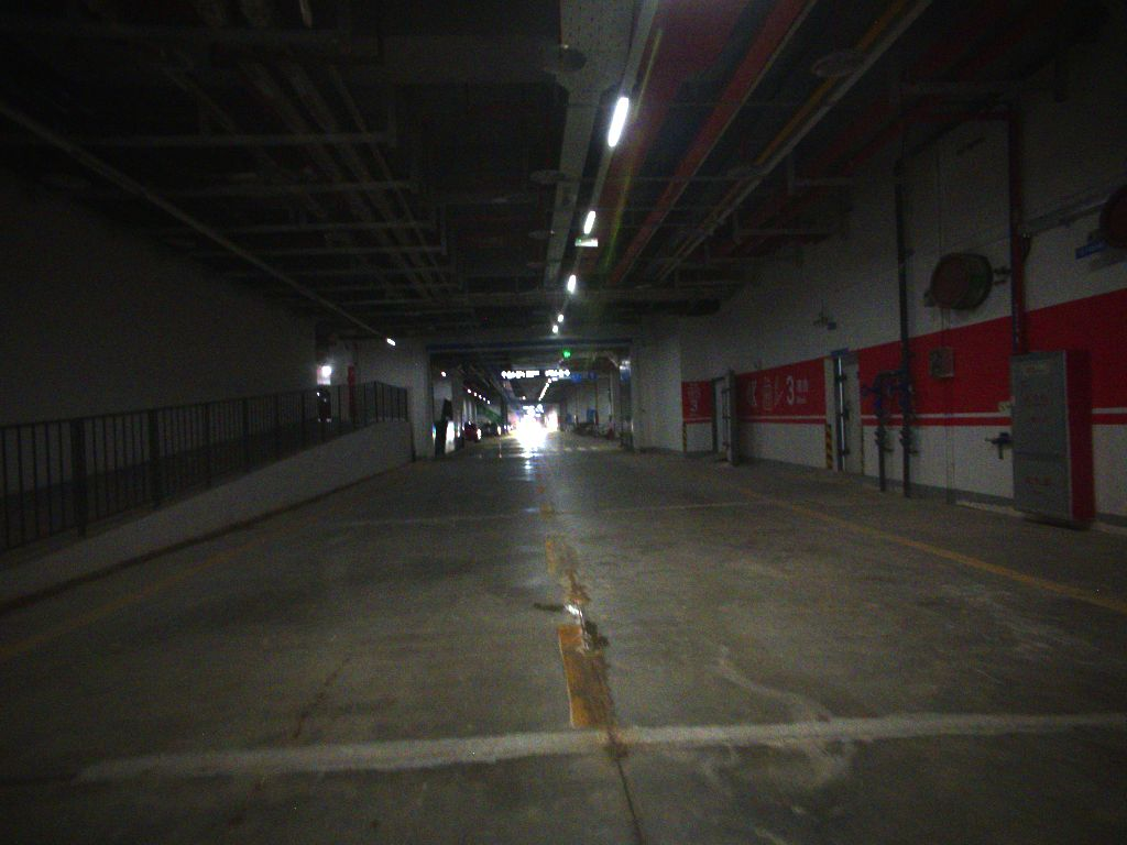
(a) The handheld multi-sensor rig and scene images covering the grassland, lab, escalator, and underground tunnel.

(b) The legged robot and scene images covering the grassland, lab, campus, and underground tunnel.

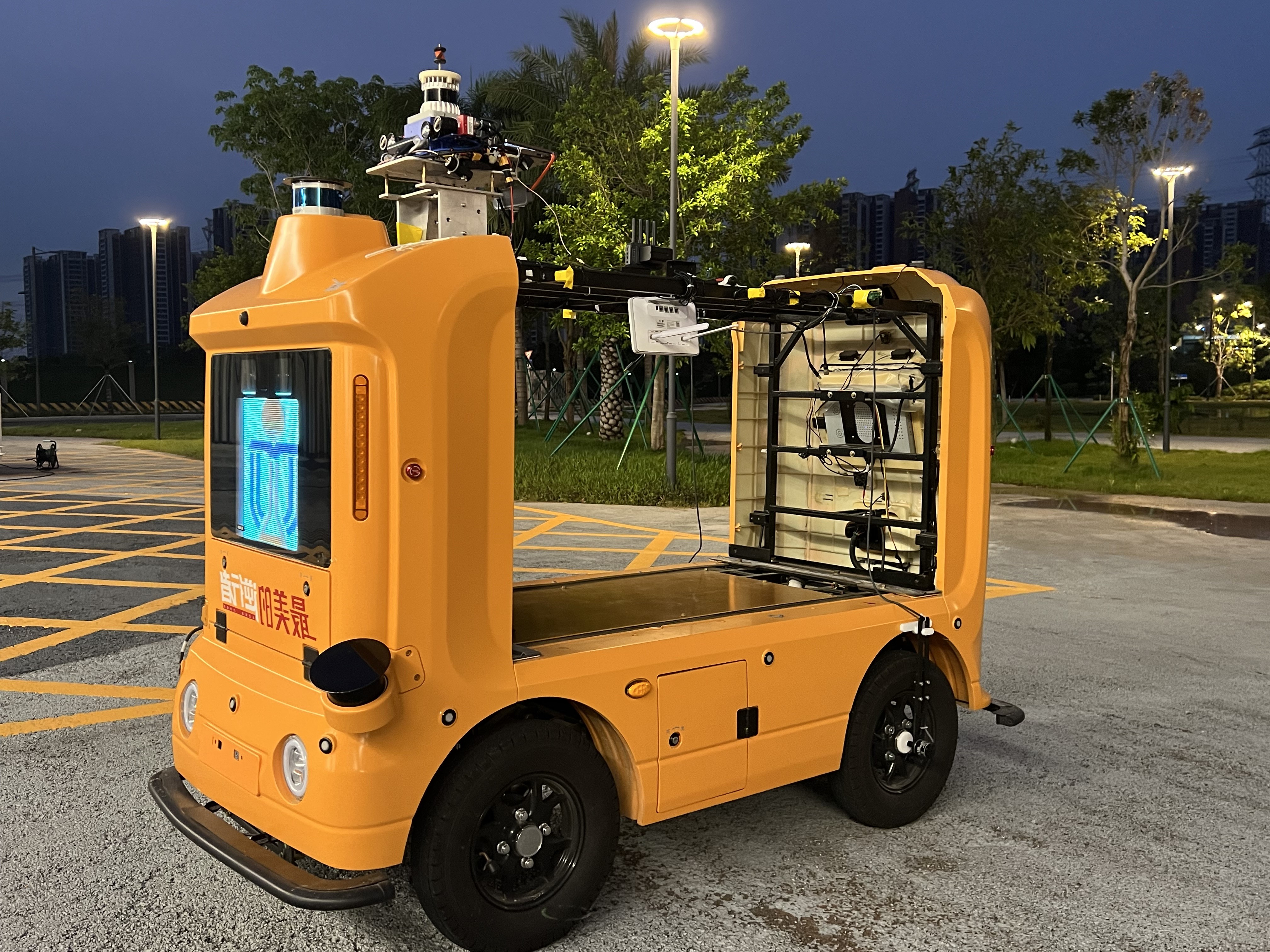
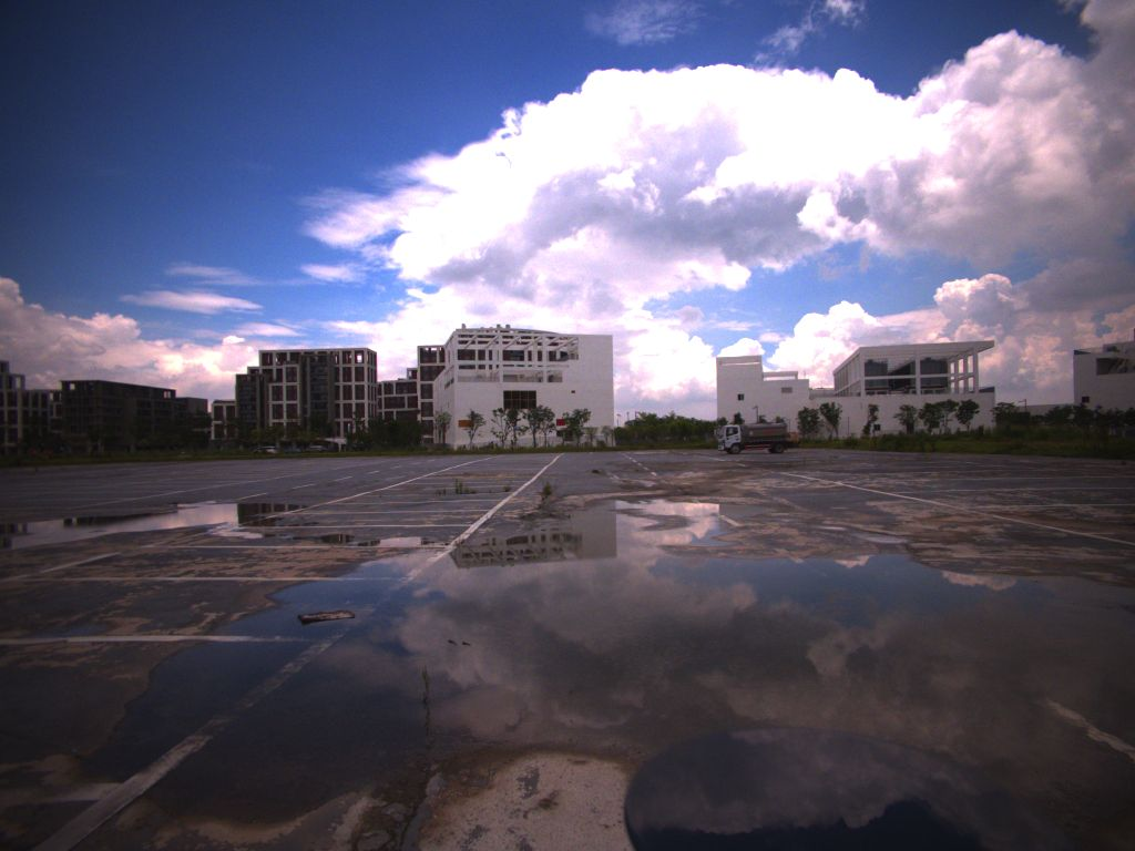
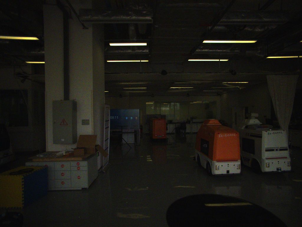
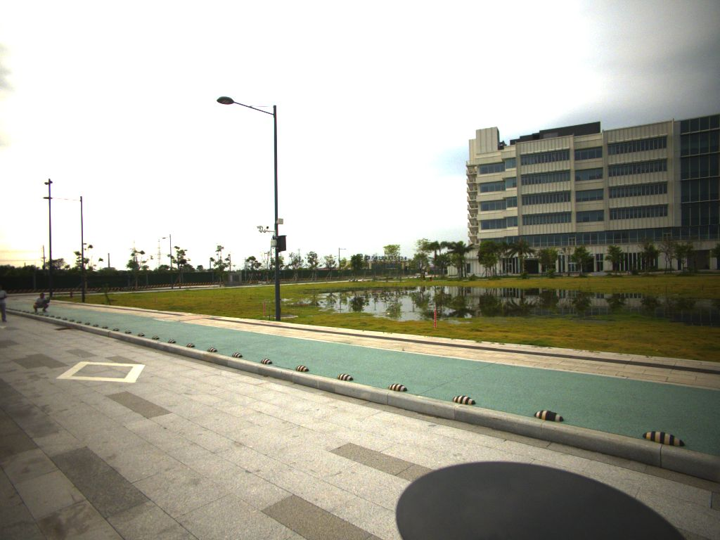
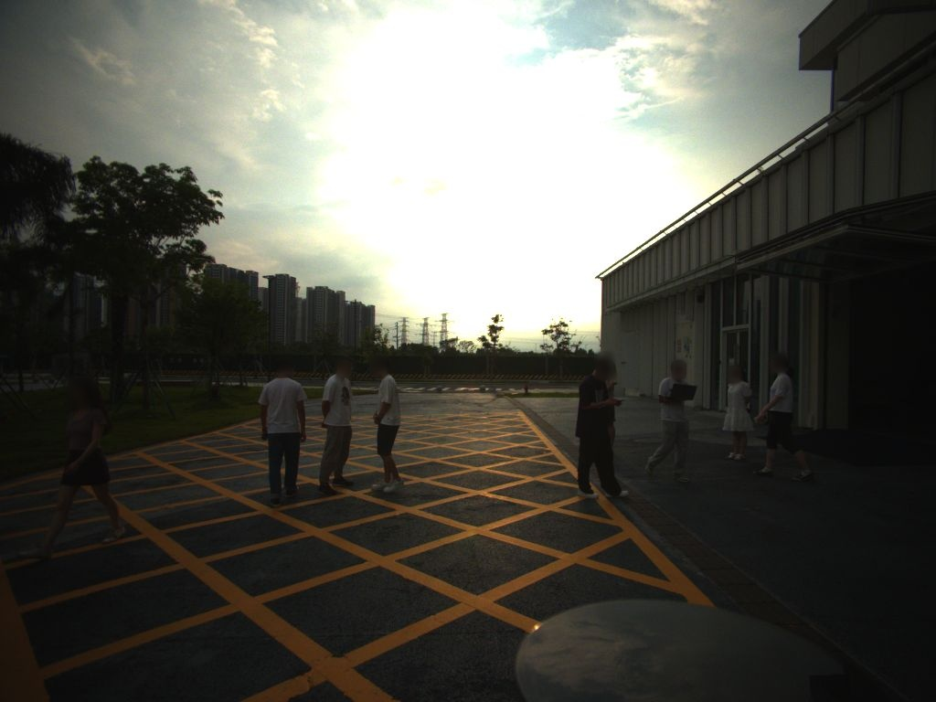
(c) The UGV and scene images covering the outdoor parking lot, garage, and campus.

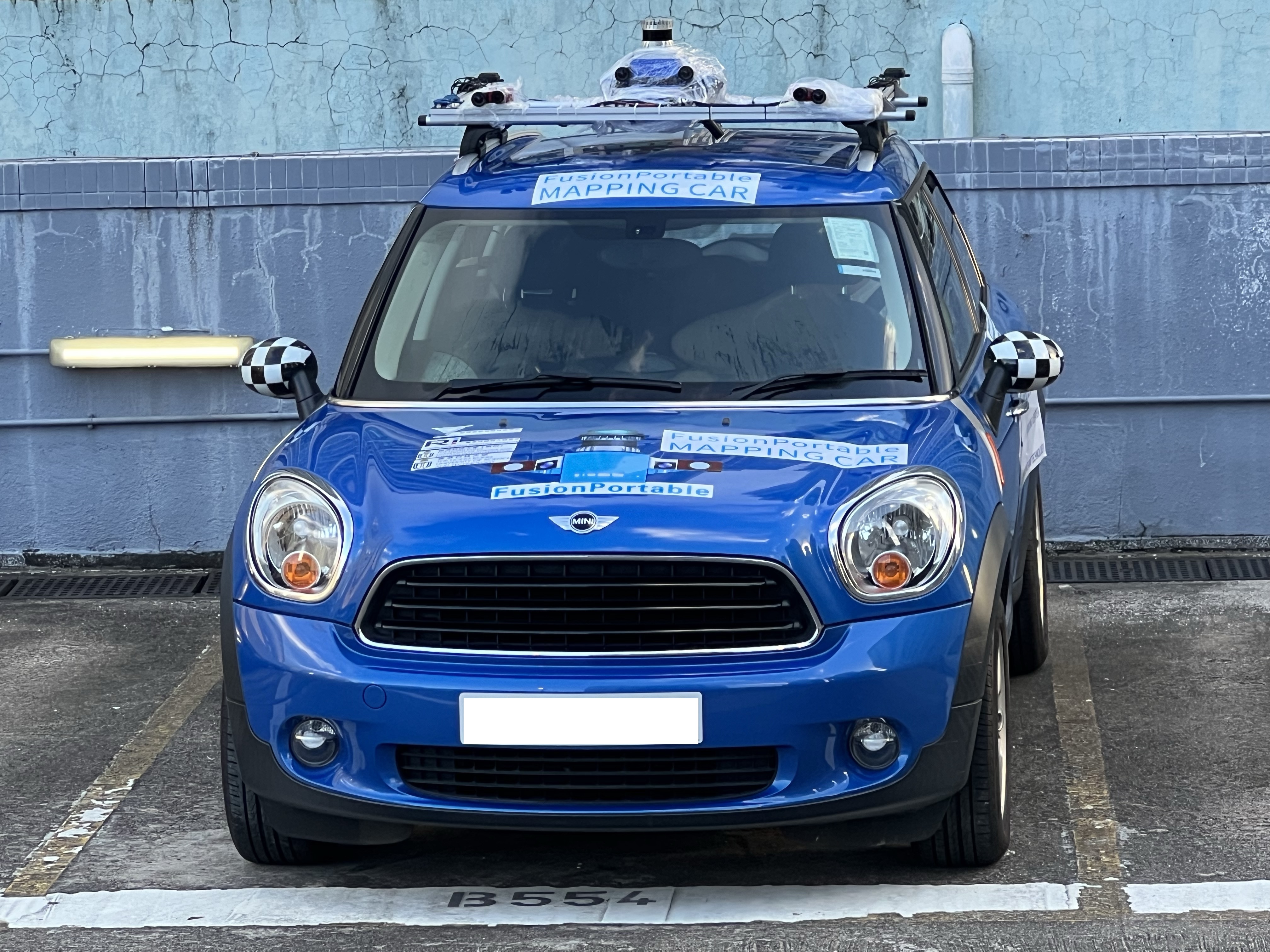
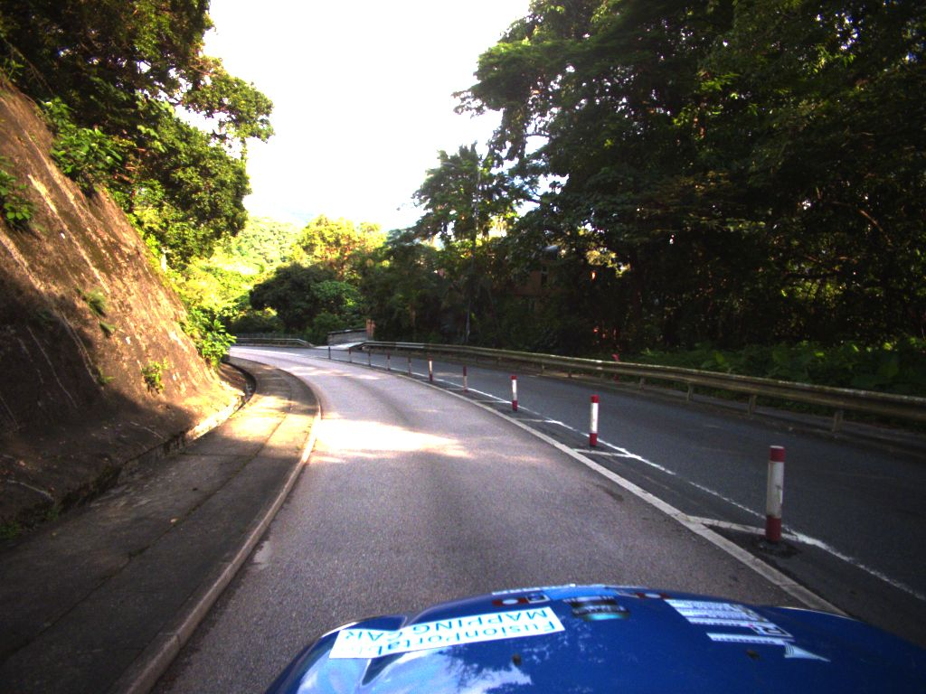
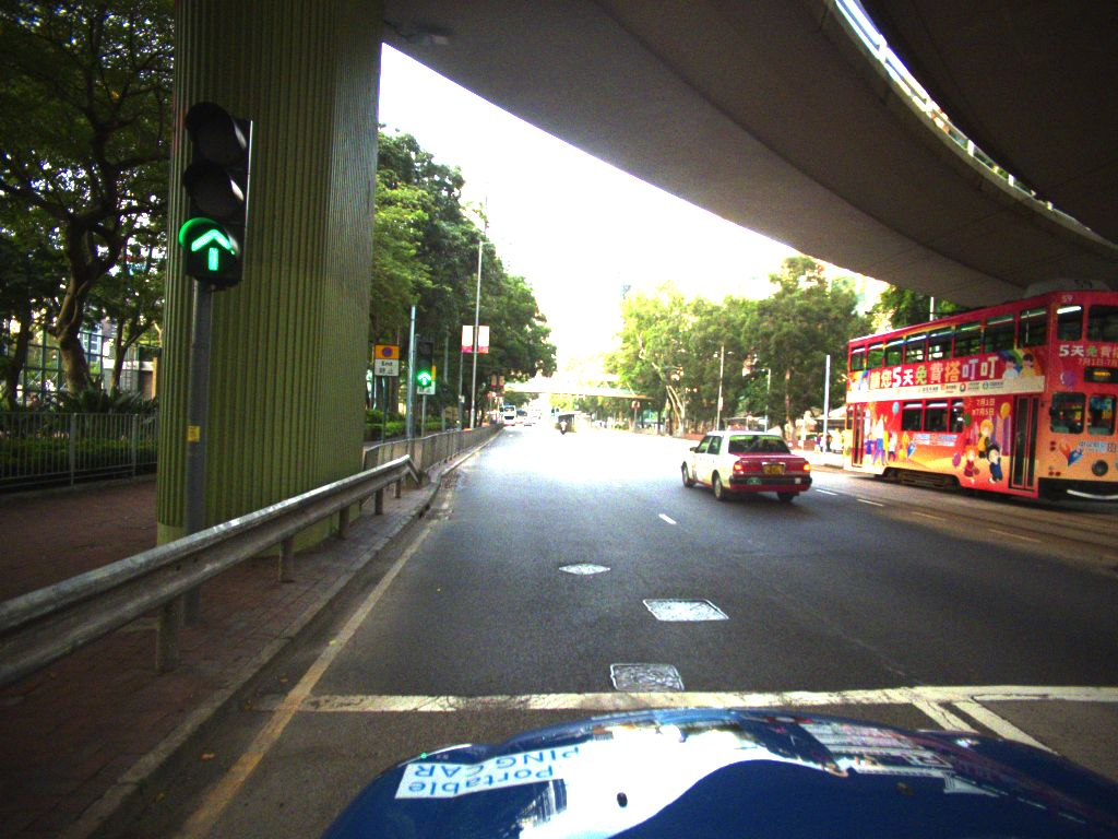
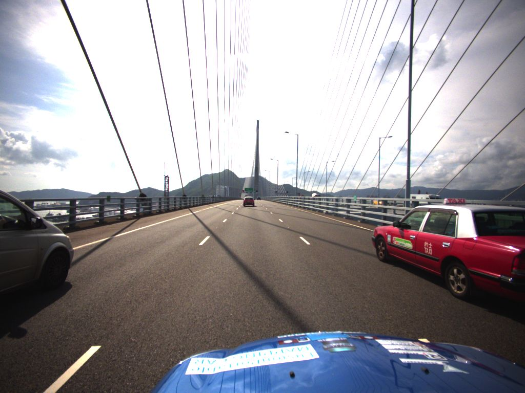
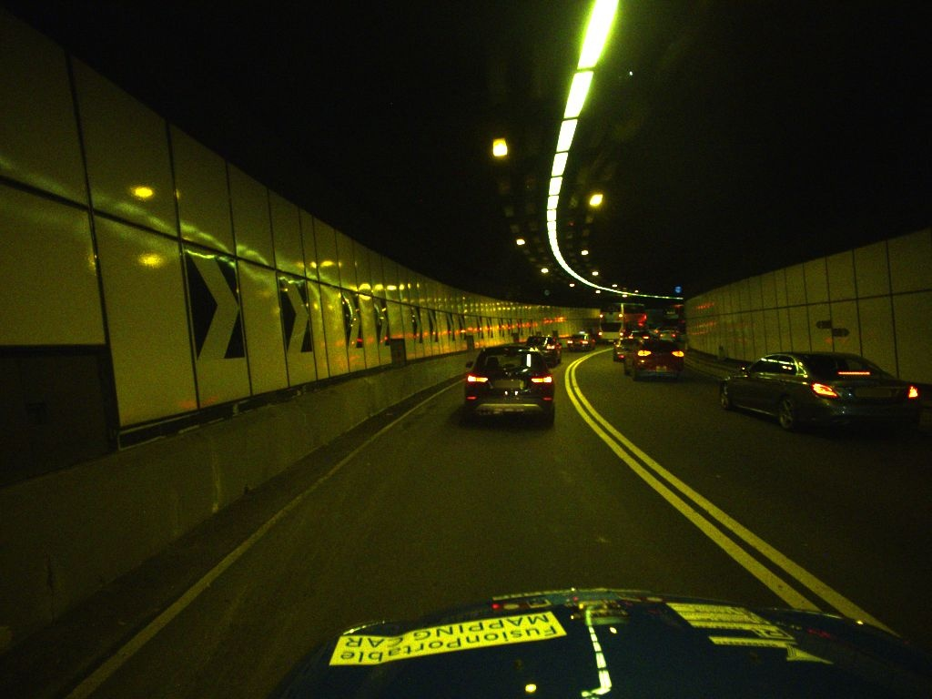
(d) The high-speed vehicle and scene images covering the mountain road, urban road, highway, and tunnel.

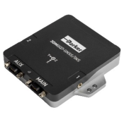
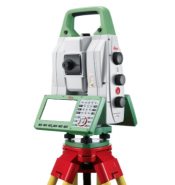
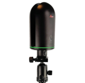
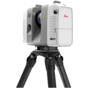
(e) Devices for generating GT trajectories and maps: $3$DM-GQ$7$, Leica MS$60$, Leica BLK$360$, and Leica RTC$360$.

Figure 4: Platform-Specific Data Samples: (a) The handheld multi-sensor rig across various environments, (b) the legged robot, (c) the low-speed UGV, (d) the high-speed vehicle, and (e) the GT generation device. The depicted scenes highlight the FusionPortableV2 dataset’s comprehensive coverage across a spectrum of platforms and environmental conditions.

3.3 Ground Truth Provision Setup

High-precision, dense RGB point cloud maps and GT trajectories are essential for evaluating SLAM and perception algorithms. This section describes three types of GT devices featured in our dataset, selected to meet the varied needs of the sequences. Through the integration of data from these GT devices, our dataset provides comprehensive support for algorithm benchmarking, not only in localization and mapping but also across diverse applications and requirements.

3.3.1 Dense RGB Point Cloud Map:

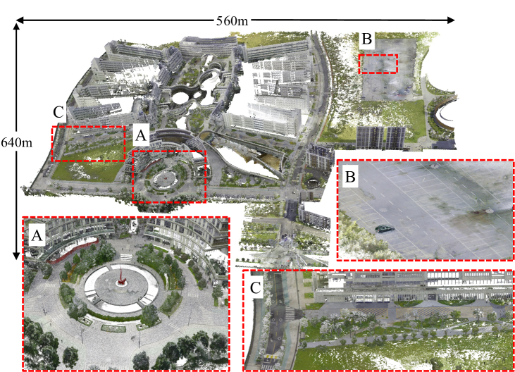
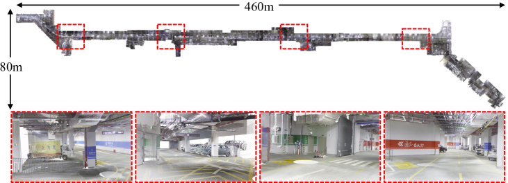
For creating dense point cloud maps of outdoor scenarios, the Leica RTC360 laser scanner was selected, known for its high scanning rate of up to $2$ million points per second and accuracy under $5.3mm$ within a $40m$ radius. Some indoor areas were scanned with the Leica BLK$360$, which operates at a rate of $0.68$ million points per second and achieves an accuracy of $4mm$ within a $10m$ range. All scans are registered and merged by the Leica Cyclone software, resulting in a dense and precise RGB point cloud map (Fig. 12). This map with the resolution as $8cm$, covering all data collection areas, can be used to evaluate the mapping results of algorithms ranging from model-based (Lin and Zhang, 2022) and learning-based methods (Pan et al., 2024).

3.3.2 3-DoF GT Trajectory:

For indoor and small-scale outdoor environments, the Leica MS$60$ total station was utilized to measure the GT trajectory of the robot at the $3$-DoF position. As shown in Fig. 4 (a), the tracking prism is placed atop the LiDAR. The GT trajectory was captured at a frequency between $5$-$8Hz$, achieving an accuracy of $1mm$. However, due to occasional instability in the measurement rate, the GT trajectory is resampled at $20Hz$ using linear interpolation for a more consistent evaluation. For further details on this process, please refer to Section 6.2.1.

3.3.3 6-DoF GT Trajectory:

While the stationary Leica MS$60$ provides accurate measurements, it cannot track the prism when it is occluded or outside the visible range. Consequently, for capturing $6$-DoF GT trajectories in large-scale and outdoor environments with available GNSS satellites, we employ the $3$DM-GQ$7$ navigation sensor. This sensor integrates data from its internal dual-antenna RTK-GNSS, which provides raw data at a frequency of $2Hz$, and an IMU, to deliver estimated poses with an output rate of up to $30Hz$. Once the GNSS has initialized with a sufficient satellite lock and RTK is in fixed status, it achieves a positioning accuracy of up to $1.4cm$.

4 Sensor Calibration

We meticulously calibrate the intrinsics of each sensor, their extrinsics, and the time offsets between certain sensors beforehand. The STIM$300$ IMU’s coordinate system is designated as the body frame, serving as the primary reference for most extrinsic calibrations. For indirectly calibrated sensors, conversion is achieved through matrix multiplication: $\bm{T}^{A}{C}=\bm{T}^{A}{B}\bm{T}^{B}_{C}$. The positioning and orientation of sensors across devices and platforms are illustrated in Fig. 1 and Fig. 3. A summary of the calibration process is provided in Table 3, with detailed results available on our dataset’s website due to page constraints.

4.1 Intrinsic Calibration

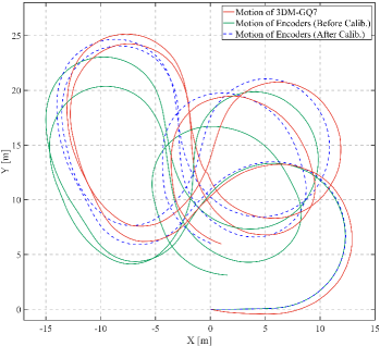
We calibrate IMUs and cameras using the off-the-shelf Kalibr toolbox Furgale et al. (2013); Rehder et al. (2016). For wheel encoder intrinsics, such as wheel radius and axle track, we implement the motion-based calibration algorithm outlined in (Jeong et al., 2019). This involves manually maneuver the UGV through significant transformations, as depicted in Fig. 6. We calculate the UGV’s planar motion for each interval $\tau\in[t_{k},t_{k+1}]$ using encoder data to determine linear ($v=(\omega_{l}r_{l}+\omega_{r}r_{r})/2$) and angular ($\omega=(\omega_{l}r_{l}-\omega_{r}r_{r})/b$) velocities. Concurrently, the $3$DM-GQ$7$ captures more accurate motion estimates. Intrinsics are then optimized by minimizing the trajectory alignment error between these two trajectories.

Table 3: Description of intrinsic and extrinsic parameter calibration.

Type	Sensor	Calibrated Parameter	Approach
Intrinsics	IMU	Noisy Density, Random Walk	Allen variance analysis Toolbox
	Wheel Encoder	Wheel Radius, Axle Track	Minimize alignment error between $\mathcal{T}_{gt}$ and $\mathcal{T}_{est}$ (Jeong et al., 2019)#
	Camera	Focal Length, Center Point, Distortion	Minimize reprojection error (Zhang, 2000)
Extrinsics	IMU-IMU	Rotation, Translation	Optimization (Rehder et al., 2016)
	IMU-Camera	Rotation, Translation, Cons. Time Offset	Optimization (Furgale et al., 2013)
	IMU-Prism	Translation	Hand-eye calibration (Furrer et al., 2018)
	IMU-Legged Sensors	Rotation, Translation	Obtained from the CAD Model
	Camera-Camera	Rotation, Translation	Minimize reprojection errors (Zhang, 2000)
	Camera-LiDAR	Rotation, Translation	Minimize point-to-line and point-to-plane errors (Jiao et al., 2023)
$\#$ detailed in the paper

Figure 5: Sensor placement for the IMU-Prism calibration. Reflective balls for motion capture cameras (MCC) and the prism are marked in red and blue, respectively. We use MCC’s measurements to infer high-rate motion of the prism.

4.2 Extrinsic Calibration

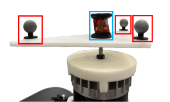
Extrinsic calibrations, encompassing $6$-DoF transformations and time offsets for IMU-IMU, IMU-camera, IMU-prism, camera-camera, and camera-LiDAR pairs, are typically obtained with off-the-shelf toolboxes. We specifically describe the calibration between the IMU and the prism that defines the reference frame of GT measurements relative to the Leica MS$60$. We design the indirect calibration method since the Leica MS$60$ provides only $3$-DoF and low-rate trajectories. We observed that the prism is visible to infrared cameras in the motion capture room. We place and adjust three tracking markers around the prism to approximate its center, as shown in Fig. 5. We move the handheld device to perform the “$8$”-shape trajectory. Both the motion capture system and LiDAR-inertial odometry (Xu et al., 2022) can estimate trajectories of the prism and STIM$300$ IMU, respectively. With these trajectories, the IMU-Prism extrinsics are estimated using the algorithm proposed in (Furrer et al., 2018).

Figure 6: Comparision of trajectories: estimated motion by the $3$DM-GQ$7$ (red), integration of encoders’ measurement before calibration (green) and after calibration (blue), respectively.

5 Dataset Description

This section begins by outlining the general motion patterns and potential applications for each platform. Following this, we consider the challenges posed by the dataset (as detailed in Section 5.2) and proceed to generate 27 sequences designed for algorithm development and evaluation (refer to Section 5.3). A summary of the essential characteristics of these sequences is provided in Table 4. In our prior publication, FusionPortable (Jiao et al., 2022), we presented more handheld and legged robot sequences captured with a similar hardware configuration but without kinematic data. This dataset encompasses 10 sequences featuring a variety of environments including garden, canteen, and escalator, captured via handheld devices, and 6 sequences obtained from a legged robot within a motion capture room.

5.1 Analysis of Platforms Characteristics

Each platform has its motion patterns (e.g., speed, angular velocity, dynamic frequency) and working ranges. Fig. 7 visualize typical motion patterns of different platforms on some example sequences. Drawing from this observation, we meticulously design sequences to highlight the unique features of each platform.

(a) Motion Analysis of the Sequence: Handheld_room00

(b) Motion Analysis of the Sequence: Legged_grass00

(c) Motion Analysis of the Sequence: Ugv_parking03

(d) Motion Analysis of the Sequence: Vehicle_highway00

Figure 7: Motion analysis with four mobile platforms in terms of acceleration $[m/s^{2}]$ and angular velocity $[rad/s]$. The left two columns of each row illustrate time-domain data, revealing immediate dynamic behaviors, while the right two columns display frequency-domain data, highlighting predominant motion features. This comparison reveals the robust requirements of general SLAM algorithms on multiple platforms.

Table 4: Statistics and key challenges of each sequence are reported. Abbreviations: T: Total time. D: Total distance traveled. L: Large. M: Medium. S: Small. $||\overline{\bm{v}}||$: Mean linear velocity. $||\bm{v}||_{\text{max}}$: Max linear velocity ($3\sigma$). 3-DoF (GNSS): Refer to Section 6.2.2. 6-DoF (SLAM): Use FAST-LIO2 (Xu et al., 2022) to generate the reference trajectory.

Platform	Sequence	T$[s]$	D$[m]$	$||\overline{\bm{v}}||/||\bm{v}||_{\text{max}}[m/s]$	Scale	Motion	Challenges	GT Pose	GT Map
Handheld	handheld_grass$00$	$140$	$80$	$0.55/1.76$	S	6-DoF Walk	Textureless	3-DoF (Tracker)	Yes
	handheld_room$00$	$140$	$63$	$0.41/1.40$	S	6-DoF Walk	Dynamic	3-DoF (Tracker)	Yes
	handheld_room$01$	$113$	$46$	$0.36/1.52$	S	6-DoF Walk	Dynamic	3-DoF (Tracker)	Yes
	handheld_escalator$00$	$247$	$95$	$0.45/1.45$	S	6-DoF Walk	Non-inertial	3-DoF (Tracker)	Yes
	handheld_escalator$01$	$254$	$88$	$0.47/1.54$	S	6-DoF Walk	Non-inertial	3-DoF (Tracker)	Yes
	handheld_underground$00$	$380$	$403$	$1.07/3.38$	M	6-DoF Walk	Structureless	3-DoF (Tracker)	Yes
Legged Robot	legged_grass$00$	$301$	$112$	$0.35/1.51$	S	Jerky	Deformable	3-DoF (Tracker)	Yes
	legged_grass$01$	$355$	$97$	$0.32/1.58$	S	Jerky	Deformable	3-DoF (Tracker)	Yes
	legged_room$00$	$173$	$57$	$0.28/1.30$	S	Jerky	Dynamic	3-DoF (Tracker)	Yes
	legged_transition$00$	$233$	$98$	$0.41/1.60$	S	Jerky	Illumination	3-DoF (Tracker)	Yes
	legged_underground$00$	$274$	$167$	$0.58/2.46$	M	Jerky	Structureless	3-DoF (Tracker)	Yes
UGV	ugv_parking$00$	$178$	$319$	$1.77/2.80$	M	Smooth	Structureless	6-DoF (INS)	Yes
	ugv_parking$01$	$292$	$434$	$1.48/4.07$	M	Smooth	Structureless	6-DoF (INS)	Yes
	ugv_parking$02$	$80$	$242$	$3.04/4.59$	M	Jerky	Structureless	6-DoF (INS)	Yes
	ugv_parking$03$	$79$	$218$	$2.75/4.92$	M	Jerky	Structureless	6-DoF (INS)	Yes
	ugv_campus$00$	$333$	$898$	$2.69/4.90$	M	Smooth	Scale	6-DoF (INS)	Yes
	ugv_campus$01$	$183$	$343$	$1.86/4.40$	M	Jerky	Fast Motion	6-DoF (INS)	Yes
	ugv_transition$00$	$491$	$445$	$1.04/3.25$	S	Smooth	GNSS-Denied	3-DoF (Tracker)	Yes
	ugv_transition$01$	$375$	$356$	$0.92/3.51$	S	Smooth	GNSS-Denied	3-DoF (Tracker)	Yes
Vehicle	vehicle_campus$00$	$610$	$2708$	$4.43/9.31$	M	Height-Change	Scale	6-DoF (INS)	No
	vehicle_campus$01$	$420$	$2086$	$4.96/8.59$	M	Height-Change	Scale	6-DoF (INS)	No
	vehicle_street$00$	$578$	$8042$	$13.90/19.52$	L	High-Speed	Dynamic	3-DoF (GNSS)	No
	vehicle_tunnel$00$	$668$	$3500$	$5.24/15.00$	L	High-Speed	LiDAR	3-DoF (GNSS)	No
	vehicle_downhill$00$	$512$	$3738$	$7.29/15.59$	L	Height-Change	Illumination	6-DoF (INS)	No
	vehicle_highway$00$	$694$	$9349$	$13.46/30.87$	L	High-Speed	Structureless	6-DoF (INS)	No
	vehicle_highway$01$	$377$	$3641$	$9.64/24.36$	L	High-Speed	Structureless	6-DoF (INS)	No
	vehicle_multilayer$00$	$607$	$1021$	$1.68/4.53$	M	Spiral	Perceptual Aliasing	6-DoF (SLAM)	No

5.1.1 Handheld:

Since the handheld MSS is commonly held by a user, it offers great flexibility for data collection scenarios. The handheld multi-sensor device provides adaptable data collection across diverse settings, akin to market counterparts like the Leica BLK$2$GO mobile scanning device, which excels in precision scanning and motion estimates. Therefore, we collect data in scenarios including a laboratory with furniture and dynamic elements, uneven grasslands, an escalator for vertical transitions, and a underground parking lot resembling long tunnels. The device performs motion influenced by the user’s walking or running, sometimes leading to camera shake and rapid directional shifts. Each sequence contains a least one loop. The average movement speed is around $2m/s$.

5.1.2 Legged Robot:

The quadruped robot carries a sensor suite and commonly operates in indoors, outdoors, and underground for missions such as rescue, inspection, and document transportation. It exhibits complex motion patterns that involve a combination of walking, trotting, and running gaits. Deformable and rugged terrain can also affect motion’s stability. Our experiments reveal that high-frequency jitters and sudden bumps are challenging to SOTA LiDAR-inertial odometry methods (Xu et al., 2022). Therefore, we believe that the integration sensor measurements from the joint motor and contact for a better motion estimation deserve further study and thus provide these data (Yang et al., 2023). The operational speed of the robot is approximately $1.5m/s$.

5.1.3 Unmanned Ground Vehicle:

The UGV is typically designed for last-mile delivery and navigates middle-scale areas like campuses and factories. Constrained by Ackermann steering geometry, the UGV executes planar and smooth movements in response to the operator’s inputs. Data collection is conducted in various environments, including an outdoor parking lot (lacking structure), a campus, and the challenging transition zones between indoor and outdoor environments (where GNSS signals are unstable). To mimic real-world complexities, commands for sudden stops and $45^{\circ}$ turns are occasionally issued. The UGV can move at speeds of approximately $5m/s$.

5.1.4 Vehicle:

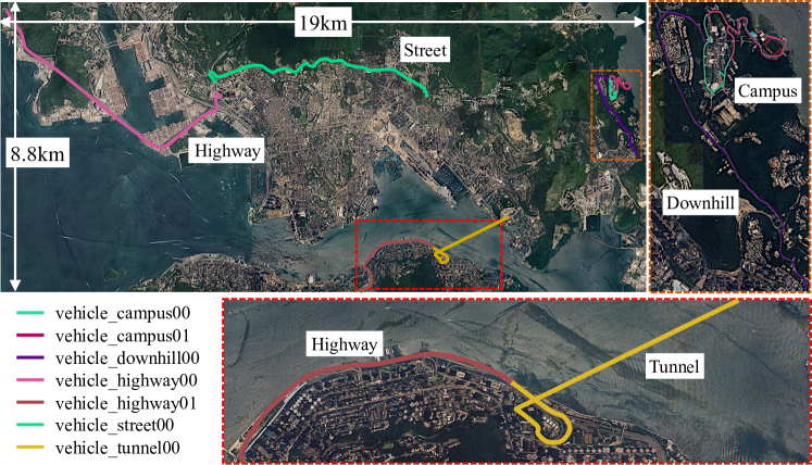
The vehicle collects data across diverse urban environments in Hong Kong, navigating through mountain roads with elevation shifts, multi-story parking lots with varying heights and orientations, dynamic downtown areas with buildings, highways, and GNSS-denied underground tunnels, which are structureless and lack distinctive textures. It operates at a range of speeds from $10km/h$ to $100km/h$, sometimes with abrupt speed and directional changes influenced by traffic and road conditions.

5.2 Challenging Factors

Prior to data collection, we acknowledge that practical factors contribute to sensor degradation and potential algorithmic failure. Our data sequences, integrated with the platforms described, aim to comprehensively evaluate algorithm performance in terms of accuracy, efficiency, and robustness. Additionally, we anticipate these sequences will potentially draw the development of novel algorithms.

5.2.1 Illumination Conditions:

Different illumination conditions, such as bright sunlight, shadows, and low light, affect the quality of visual sensors and pose challenges for visual perception algorithms. For example, in bright sunlight, cameras are sometimes overexposed, resulting in a loss of appearance information. On the contrary, cameras are sometimes underexposed in low light conditions, leading to image noise and poor visibility.

5.2.2 Richness of Texture and Structure:

Structured environments can mainly be explained using geometric primitives (e.g., offices or buildings), while semi-structured environments have both geometric and complex elements like trees and sundries. Scenarios like narrow corridors are structured but may cause state estimators. Additionally, texture-rich scenes facilitate visual algorithms to extract stable features (e.g., points and lines), while texture-less may negatively affect the performance. Also, in texture-less environments, only a small amount of events are triggered.

5.2.3 Dynamic Objects:

In dynamic environments, several elements (e.g., pedestrians or cars) are moving when the data are captured. This is in contrast to static environments. For instance, moving cars cause noisy reflections and occlusions to LiDAR data, while pedestrians cause motion blur to images. Overall, dynamic objects induce negative effects from several aspects such as incorrect data association, occlusion, and “ghost” points remaining on the map.

Figure 8: The dataset organization.

(a) Handheld_escalator00

(b) Vehicle_campus00

Figure 9: Projected point cloud onto the left frame image with our SDK. Points’ color indicate the relative distance. This involves basic implementation including data loader, calibration loader, point cloud manipulation, and camera model.

5.2.4 Intermittent GNSS:

The intermittent GNSS signal issue typically arises in environments like places where dense and towering urban clusters are presented, overpasses, and indoor-outdoor transition areas. A special example is the city center of Hong Kong. In such scenarios, GNSS signals are often obstructed, leading to sporadic reception and significant uncertainty.

Figure 10: Trajectories of several sequences collected using the low-speed UGV in the campus, where environments with different structures and texture including room, escalator, grassland, parking lots are presented.

Figure 11: Trajectories of several sequences collected using the high-speed vehicle in Hong Kong.

5.2.5 Scale Variability:

Developing SLAM and perception algorithms for large-scale environments may encounter challenges such as an increased computational load and a heightened risk of perceptual aliasing. The former necessitates stricter demands on algorithm latency and memory usage, whereas the latter requires more accurate long-term associations for place recognition (Lowry et al., 2015), given the potential for environments to include geographically distant yet visually similar locations.

5.3 Sequence Description

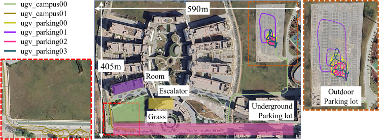
Table 4 summarizes the characteristics of our proposed sequences, detailing aspects such as temporal and spatial dimensions, motion patterns, locations, textural and structural richness, and whether GT poses and maps cover. Fig. 10 and 11 illustrate the coverage areas of the sequences from a satellite view perspective.

(a) Campus

(b) Underground Parking Lot

Figure 12: GT RGB point cloud map of the (a) campus ($\approx 0.36km^{2}$) and (b) the underground parking lot ($\approx 0.037km^{2}$) with $4mm$-resolution. It almost encompasses the range of most sequences except for those related to vehicles. For detailed map information, please refer to our video presentation.

5.4 Dataset Organization

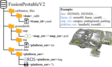
Fig. 8 outlines our dataset’s organization. Sensor data were captured using the ROS bag tool. To facilitate download, ROS bags were compressed with 7-Zip. Each bag follows the naming convention $<$platform_env$>$. Sensor calibration parameters are saved in yaml files corresponding to their coordinate frames, such as frame_cam00.yaml for the left camera and frame_cam01.yaml for the right. Given the $6$-month dataset construction period, calibration was performed and documented multiple times, with parameters organized by calibration date (e.g., 20230426_calib). Sequences must utilize the appropriate calibration files and such correspondences are provided in the development package. GT poses at the TUM format are recorded in files matching the sequence names, detailing timestamp, orientation (as Hamilton quaternion), and translation vector per line. GT map at $8cm$ resolution is provided as the pcd format, naming as $<$map_env$>$. Please note that all the data provided have undergone additional post-processing steps, following the procedures detailed in Section 6.

5.5 Development Tools

We release a set of tools that enable users to tailor our dataset to their specific application needs. Components are introduced as follows:

5.5.1 Software Development Kit (SDK):

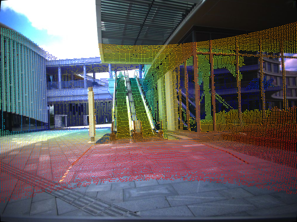
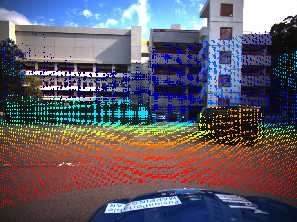
We present a Python-only SDK that is both extensible and user-friendly. The kit includes foundational functions such as loading calibration parameters and visualizing them using a TF tree, parsing ROS messages into discrete files, data post-processing, and basic data manipulation). Fig. 9 shows the point cloud projection function provided by the package.

5.5.2 Evaluation:

We provide a set of scripts and tools for algorithm evaluation including localization and mapping.

5.5.3 Application:

We provide open-source repositories for users to try different applications with our dataset covering localization, mapping, monocular depth estimation, and anonymization of specific objects. All can be found on the dataset website.

6 Data Post-Processing

The raw data captured by sensors and GT devices undergo post-processing before public release. The specifics are outlined as follows.

(a) Optimal Offset Enumeration

(b) Without Time Offset Correction

(c) With Time Offset Correction

Figure 13: Alignment process for handheld_escalator00 sequence. (a) deplicts the ATE versus time offset, pinpointing the optimal offset at $-0.64s$. (b) and (c) illustrate the $Z$-axis trajectories for the first $200$ seconds, before and after alignment, respectively, highlighting the applied time offset correction.

6.1 Privacy Management

Data collection in public spaces such as the campus and urban roads was conducted with strict adherence to privacy regulations. We employed the anonymization technique introduced in (Burnett et al., 2023) to obscure all human faces and license plates in images from our stereo frame cameras. Building upon the original implementation, we enhanced the algorithm’s efficiency using the ONNX Runtime Library. This upgraded version is now ROS-compatible, offering a valuable resource to the community, and is included in our development tools.

6.2 GT Data Processing

Due to diverse sources of GT trajectories and maps, it is necessary to standardize the GT data through processing and conversion and then verify them. These steps should be executed sequentially.

6.2.1 3-DoF GT Poses of MS60:

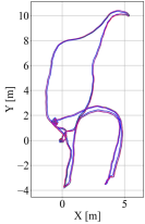
The preprocessing initiates with temporal alignment, crucial for synchronizing Leica MS60 total station measurements with sensor data, following the approach proposed in (Nguyen et al., 2022). This synchronization finds the optimal time offset ($\delta$) that minimizes the Absolute Trajectory Error (ATE) between the MS$60$’s recorded poses $\mathcal{T}_{ms60}$ and the SLAM-generated poses $\mathcal{T}_{alg}$. This is done by enumerating offsets at intervals of $0.01s$ to generate various versions of time-shifted poses from the total station poses, as shown in Fig. 13. Upon adjusting their timestamps with the optimal $\delta$, all MS$60$ poses (recorded at $5$-$8Hz$) are resampled to a denser $20Hz$ sequence via cubic spline interpolation. This method not only yields a smooth, continuous trajectory but also synchronizes the data with SLAM algorithm outputs temporally. To maintain interpolated data accuracy, intervals longer than $1s$, potentially signifying obstructions, are omitted from the sequence.

6.2.2 6-DoF GT Poses of 3DM-GQ7:

Each $6$-DoF pose provided by the INS is accompanied by a variance value, indicating the measurement’s uncertainty. This uncertainty increases when the GNSS signal is obstructed. We provide the original data along with tools designed to remove data points with excessive covariance, ultimately converting them into the TUM format. For sequences where intermittent GNSS signals disrupt the INS odometry filter convergence (denoted as sequences vehicle_street00 and vehicle_tunnel00), we recommend using the original GNSS data sampled at $2Hz$, providing 3-DoF GT poses instead.

6.2.3 Quality Analysis of GT Maps:

In constructing our GT maps, we utilized a high-precision Leica scanner for both indoor and outdoor environments. The resulting consolidated RGB point clouds comprise $289$ scanning stations and $342$ inter-scan links, as depicted in Fig. 12. We leveraged Leica Cyclone software for quality assessment of the merged GT maps, resulting in an average error of less than $15mm$ across all pairwise scans, with $90\%$ of these scans having an error of $10mm$ or less. These findings confirm that the precision of GT map far exceeds that of LiDAR-inertial odometry (typically $30mm$), validating its use for evaluation purposes.

7 Experiment

We manually select $8$ representative sequences ($2$ sequences from each platform) from the dataset to conduct a series algorithm evaluation and verification. Experiments include localization, mapping, and monocular depth estimation.

7.1 Evaluation of Localization

7.1.1 Experiment Setting:

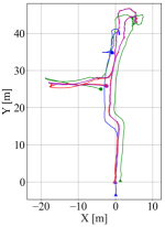
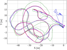
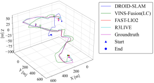
As one of the main applications, this dataset can be used to benchmark SOTA SLAM algorithms. Here in, for evaluation of robust localization systems with different input modalities, we carefully select four SOTA SLAM algorithms (including a learning-based method): DROID-SLAM (left frame camera) (Teed and Deng, 2021), VINS-Fusion(LC) (IMU+stereo frame cameras+loop closure) (Qin et al., 2018), FAST-LIO2 (IMU+LiDAR) (Xu et al., 2022), and R3LIVE (IMU+LiDAR+left frame camera) (Lin and Zhang, 2022). The customized data loaders of each evaluated method will be publicly released to foster research.

(a) handheld_room00

(b) legged_grass00

(c) ugv_parking00

(d) vehicle_campus00

Figure 14: This figure illustrates the comparative performance of leading SLAM algorithms operating across four distinct platforms and environmental contexts, from indoor spaces to a university campus. It is evident that LiDAR-based methods such as FAST-LIO2 and R3LIVE consistently outperform their vision-based counterparts across all scenarios, maintaining a higher trajectory accuracy. On the other hand, the performance of vision-based algorithms, particularly DROID-SLAM, deteriorates as the environment scale increases, with significant scale recovery issues observed in the expansive vehicle_campus00 sequence. This trend underscores the superior robustness of LiDAR-based SLAM in varied and large-scale environments.

Table 5: Localization accuracy: we calculate translation ATE $[m]$ for each sequence.

Sequence	R3LIVE	FAST- LIO2	VINS- Fusion (LC)	DROID- SLAM
handheld_room$00$	$\bm{0.057}$	$0.058$	$0.063$	$0.118$
handheld_escalator$00$	$0.093$	$\bm{0.085}$	$0.258$	$4.427$
legged_grass$00$	$\bm{0.069}$	$0.327$	$1.801$	$7.011$
legged_room$00$	$\bm{0.068}$	$0.093$	$0.149$	$0.135$
ugv_campus$00$	$\bm{1.486}$	$1.617$	$1.866$	$43.869$
ugv_parking$00$	$0.424$	$\bm{0.271}$	$2.400$	$2.019$
vehicle_campus$00$	$10.070$	$\bm{8.584}$	$66.428$	$\times$
vehicle_highway$00$	$\times$	$686.940$	$\times$	$\times$

Marching from traditional to deep learning-based SLAM methods, we evaluate DROID-SLAM, an end-to-end deep visual SLAM algorithm. We employ DROID-SLAM on the monocular image stream with a pre-trained model without fine-tuning to present a fair comparison to model-based methods. Meanwhile, testing the limits of its generalization ability is crucial for SLAM. The pre-trained model is trained by supervision from optical flow and poses on the synthetic dataset TartanAir (Wang et al., 2020), covering various conditions (e.g., appearance and viewpoint changes) and environments (e.g., from small-scale indoor to large-scale suburban). All the experiments are conducted on NVIDIA GPU GeForce RTX 3090 with a downsampled image resolution of $320\times 240$. The average runtime is $16$ FPS with a global bundle adjustment (BA) layer. The average GPU memory consumption is below $11$ GB.

7.1.2 Evaluation:

We choose the typical evaluation metric: mean ATE to evaluate the accuracy of estimated trajectories against the GT using the EVO package. Table 5 reports the quantitative localization results.

In our evaluation of SOTA SLAM systems, we observed that each system’s performance is closely tied to its sensor configuration and algorithmic approach, as outlined in our experimental settings. The analysis, reflected in Table 5, reveals insights into the adaptability and precision of these systems across various environments. Due to the precise geometric information inherent in LiDAR raw data, methods incorporating LiDAR generally exhibit higher accuracy. However, as scene scale increases and becomes more complex (like the highway), segments lacking visual texture or structural features become challenging. FAST-LIO2, which utilizes IMU and LiDAR data, showcased robust performance across a diverse array of environments. This highlights the inherent strength of LiDAR-based systems in tackling various and complex scenarios. In contrast, R3LIVE, which integrates IMU, LiDAR, and visual data, consistently demonstrated superior accuracy in different settings, particularly outperforming FAST-LIO2 in scenarios where LiDAR degradation and jerky motion pattern are present (e.g., ugv_campus00, legged_grass00). However, in environments featuring intricate visual features such as water surfaces or reflective glass on the ugv_parking00, the presence of visual mechanisms in R3LIVE may lead to a performance decrease.

For vision-based methods, VINS-Fusion outperforms DROID-SLAM on average, demonstrating robustness and generalization ability over learning-based methods. In the meantime, it is worth noting that DROID-SLAM with only monocular input beats VINS-Fusion on three sequences: handheld_room00, legged_room00, and ugv_parking00. Compared with the rest of the sequences, these three sequences are of smaller scale with constraint boundaries (i.e., a closed environment). Nevertheless, this result presents promising potential for employing deep learning in SLAM algorithms. With the recent advent of visual foundation models (Oquab et al., 2023), we might be able to unleash the power of data-driven methods to build an accurate and general SLAM foundation model.

These findings emphasize the importance of sensor diversity and well-designed fusion techniques in SLAM systems to address the variability and complexity of real-world environments.

Figure 15: Map Evaluation of FAST-LIO2 Across Diverse Scenarios. This figure presents the mapping performance of FAST-LIO2 in various environments: (a) ugv_campus00, (b) handheld_escalator00, (c) legged_grass01, (d) ugv_parking00, (e) handheld_room00, and (f) legged_room00. The color gradient, from red to blue, illustrates the range of errors in the map points generated by FAST-LIO2, with red indicating higher errors (up to $20\text{\,}\mathrm{c}\mathrm{m}$) and blue denoting lower errors (down to 0), where deeper blue signifies higher mapping precision. Notably, (a) shows significant z-axis drift in an outdoor large-scale scenario, resulting in predominantly high-error red areas in the map evaluation. Conversely, (f) Illustrates the algorithm’s application on a quadruped platform in an indoor office environment characterized by intense ground movement, glass-induced noise, and numerous dynamic obstacles, which are depicted by the red areas signifying higher error.

Figure 16: This figure demonstrates the map evaluation results within the handheld_room00 dataset using R3LIVE. The estimated point cloud map is compared against the ground truth map, with the color gradient from blue to red indicating accuracy discrepancies ranging from 0 to $20\text{\,}\mathrm{c}\mathrm{m}$. The inset highlights significant errors in the seating area within the room.

7.2 Evaluation of Mapping

Localization and mapping represent the foundational tasks for robotic navigation, and evaluating trajectory accuracy alone does not suffice to encapsulate the efficacy of such processes comprehensively. Within the framework of SLAM algorithms predicated on Gaussian models, the map serves as an estimand, and its accuracy assessment indirectly mirrors the precision of localization. For the broader spectrum of mapping tasks, whether conducted online or offline, sparse or dense, direct evaluation of map accuracy remains crucial. Hence, a module dedicated to assessing map accuracy has been developed to address this need, ensuring a holistic appraisal of navigational competencies.

7.2.1 Experiment Setting:

For GT map acquisition, high-precision dense RGB point cloud maps were collected using a Leica scanner, with point clouds sampled using a voxel grid $8cm$. Point cloud maps of these sequences were estimated using a SLAM algorithm, with single frame map point clouds sampled at a $10cm$ voxel grid and the aggregated point cloud map of stitched single frames sampled at a $1cm$ grid. Initial transformations for aligning the estimated maps to the GT maps were obtained using CloudCompare. Finally, a correspondence threshold of $20cm$ was established to quantify error metrics, facilitating a rigorous assessment of map accuracy and fidelity.

7.2.2 Evaluation:

Table 6: Mapping accuracy: we calculate four metrics to evaluate FAST-LIO2 (FL2) and R3LIVE (R3L)

Sequence	RE $[m]$		COM $[\%]$		CD $[m]$
	FL2	R3L	FL2	R3L	FL2	R3L
handheld_room$00$	$\bm{0.144}$	$0.269$	$\bm{0.949}$	$0.802$	$\bm{0.109}$	$0.131$
handheld_escalator$00$	$\bm{0.273}$	$0.544$	$\bm{0.846}$	$0.340$	$0.128$	$\bm{0.126}$
legged_grass$00$	$\bm{0.092}$	$0.199$	$\bm{0.818}$	$0.406$	$\bm{0.158}$	$0.161$
legged_room$00$	$0.442$	$\bm{0.196}$	$\bm{0.445}$	$0.316$	$\bm{0.132}$	$0.163$
ugv_campus$00$	$\bm{0.765}$	$0.767$	$\bm{0.232}$	$0.217$	$0.112$	$\bm{0.107}$
ugv_parking$00$	$\bm{0.105}$	$0.122$	$\bm{0.956}$	$0.567$	$\bm{0.110}$	$0.166$

Figure 17: This figure shows the unsupervised depth prediction results of our baseline method generalized over different system configurations.

Table 7: Performance of FSNet MonoDepth (Liu et al., 2023) on FusionPortableV2. Results are categorized by the training domain and testing domain. The left four metrics: ARD, SRD, RMSE-linear, and RMSE-log are error metrics (the lower the better). The right three metric: $\delta<\delta_{thr}$ are accuracy metrics (the higher the better).

Modals	Test Sequences	ARD	SRD	RNSE-linear $[m,\downarrow],$	RNSE-log	$\delta<1.25\ [\%,\uparrow]$	$\delta<1.25^{2}\ [\%,\uparrow]$	$\delta<1.25^{3}\ [\%,\uparrow]$
FSNet-Handheld	Handheld	$0.592$	$7.885$	$5.750$	$0.552$	$0.440$	$0.697$	$0.825$
	Vehicle	$0.235$	$1.724$	$5.210$	$0.287$	$0.670$	$0.887$	$0.961$
FSNet-Vehicle	Handheld	$1.031$	$15.786$	$6.970$	$0.742$	$0.300$	$0.531$	$0.679$
	Vehicle	$\bm{0.125}$	$\bm{1.522}$	$\bm{4.561}$	$\bm{0.199}$	$\bm{0.882}$	$\bm{0.955}$	$\bm{0.978}$

We follow (Hu et al., 2024) to use these metrics for mapping evaluation, as a complement to localization evaluation. In the presence of high-precision RGB point cloud map ground truth, the accuracy of the maps reconstructed by the algorithm can be evaluated. We register the estimated point cloud map $\mathcal{M}$, reconstructed by the algorithm, to the ground-truth point cloud map $\mathcal{G}$, subsequently obtaining the corresponding set of associated points. By computation of precision metrics on this set of associated points, we can also mitigate minor map variations due to temporal discrepancies in ground-truth point cloud collection and slight interference from dynamic obstacles. We compare these two maps based on four metrics: Reconstruction Error (RE) in terms of the Root Mean Squared Error (RMSE), Completeness (COM), and Chamfer Distance (CD). They are defined as below:

• Reconstruction Error computes the average point-to-point distance between $\mathcal{M}$ and $\mathcal{G}$ (Pan et al., 2022):

  $$\textit{RE}=\sqrt{\frac{1}{|\mathcal{M}|}\sum_{\bm{p}\in\mathcal{M}}{\underbrace{\min(\tau,\ \|\bm{p}-\bm{q}\|)}_{d(\bm{p},\mathcal{G})}}^{2}},$$ (1)

  where $\tau$ is the inlier distance and $\mathbf{q}\in\mathcal{G}$ is the nearest point to $\mathbf{q}$. We empirically set $\tau=0.2m$ in experiments.

• Completeness is equal to $\mathrm{COM}=|\mathcal{G}^{\prime}|/|\mathcal{G}|$ that describes how does $\mathcal{M}$ cover extent of $\mathcal{G}$. $\mathcal{G}^{\prime}$ is the subset of $\mathcal{G}$. Each element of $\mathcal{G}^{\prime}$ has a nearby point from $\mathcal{M}$ such as

  $$\textit{COM}=\{\mathbf{q}\in\mathcal{G}^{\prime}\ |\ \ \ \exists\mathbf{p}\in\mathcal{M},||\mathbf{p}-\mathbf{q}||\leq\tau\}.$$ (2)

• Chamfer Distance computes the Chamfer-L1 Distance (Mescheder et al., 2019) as:

  $$\textit{CD}=\frac{1}{2|\mathcal{M}|}\sum_{\bm{p}\in\mathcal{M}}d(\bm{p},\mathcal{G})+\frac{1}{2|\mathcal{G}|}\sum_{\bm{q}\in\mathcal{G}}d(\bm{q},\mathcal{M}).$$ (3)

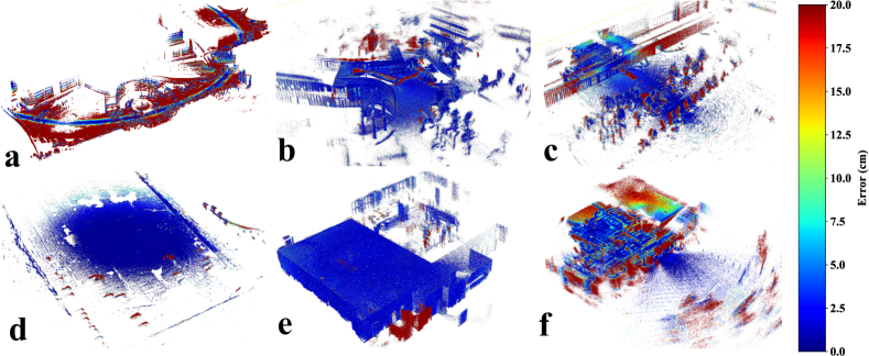
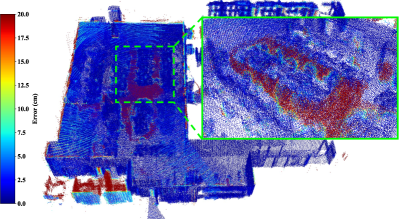
Fig. 15 employs the map evaluation module to present the assessment outcomes of the FAST-LIO algorithm across six indoor and outdoor data sequences, with varying colors representing the accuracy levels across different map regions. The map accuracy estimated by FAST-LIO notably decreases in outdoor large-scale scenes (Fig. 15 (a)) or areas with dense vegetation (Fig. 15 (c) and Fig. 15 (f)), attributable to significant measurement noise from trees or overall z-axis drift in outdoor LiDAR Odometry and Mapping applications. Conversely, indoor settings, barring the effects introduced by dynamic obstacles (Fig. 15 (f)), predominantly exhibit high map quality (Fig. 15 (e)).

Table 6 further delineates the map evaluation results for F2L and R3L across six indoor and outdoor sequences, with R3L retaining only points with RGB colors, hence showing inferior performance on the COM metric compared to F2L. However, F2L outperforms R3L in most scenes in terms of RE and CD metrics, particularly in handheld and quadruped robot sequences. In expansive campus environments, both algorithms exhibit comparable CD metrics, as seen in scenarios like handheld_escalator and ugv_campus. Fig. 16 illustrates the mapping results of R3LIVE on the handheld_room00 sequence, employing a color scheme consistent with that of Fig. 15. The presence of glass within the room introduces noise, resulting in some blurred regions within the map. This depiction underscores the impact of environmental features on mapping clarity.

7.3 Evaluation of Depth Estimation

The diversity of sensors, mobile platforms, and scenarios make our dataset appealing for algorithm verification not limited to localization and mapping. In this section, we demonstrate that our dataset can serve for the evaluation of advanced perception algorithms. Due to the easily accessible GT, we set the benchmark for measuring the generalization ability of unsupervised monocular depth prediction. The benchmark measures how unsupervised monocular depth prediction networks could perform on scenes collected from different data collection platforms.

7.3.1 Data Preparation:

Each frame image is accompanied by a GT depth image of identical size for evaluation. Depth images are produced by projecting point clouds, generated by FAST-LIO2 (Xu et al., 2022) through IMU interpolastion, onto these frames:

$$D_{gt}(\mathbf{x})=Z,\ \ \ \mathbf{x}=\lfloor\pi(\mathbf{p}^{c})\rceil,\ \ \ \mathbf{p}^{c}=\mathbf{R}^{c}_{l}\mathbf{p}^{l}+\mathbf{t}^{c}_{l},$$ (4)

where $Z$ is the $z$-axis value of $\mathbf{p}^{c}$, $\pi(\cdot)$ is the camera projection function, $\lfloor\cdot\rceil$ is the rounding operation, and $(\mathbf{R}^{c}_{l},\mathbf{t}^{c}_{l})$ represents the extrinsics from the left frame camera to the LiDAR.

7.3.2 Experiment Setting:

Monocular depth estimation tests are essential for evaluating a system’s ability to perceive relative object distances from a single camera view, a key aspect of understanding spatial relationships. Based on the FSNet baseline depth estimation modal (Liu et al., 2023), we fine-tune the modal with our dataset. We organize the train-validation data into two groups. The first group allocates $70\%$ of handheld indoor sequence data (i.e., handheld_room00 and handheld_escalator00) for training, and combines $30\%$ of this data with all vehicle-related outdoor sequences for validation. The second group uses $70\%$ of vehicle sequence data (i.e., vehicle_campus00 and vehicle_parking00) for training, and blends $30\%$ of this data with all handheld sequences for validation. We train the FSNet with these groups of data respectively and obtain two modesls: FSNet-Handheld and FSNet-Vehicle.

7.3.3 Evaluation:

We assess models’ performance of unsupervised monocular depth prediction models use the proposed scale-invariant metrics in (Eigen et al., 2014): Absolute Relative Difference (ARD), Squared Relative Difference (SRD), Root Mean Squared Error (RMSE)-linear, RMSE-log, and Threshold. These metrics are defined as follow:

ARD $$=\frac{1}{|\mathcal{X}|}\sum_{\mathbf{x}\in\mathcal{X}}|d_{est}-d_{gt}|/d_{gt},$$ (5)

SRD $$=\frac{1}{|\mathcal{X}|}\sum_{\mathbf{x}\in\mathcal{X}}\|d_{est}-d_{gt}\|^{2}/d_{gt},$$

RMSE-linear $$=\sqrt{\frac{1}{|\mathcal{X}|}\sum_{\mathbf{x}\in\mathcal{X}}\|d_{est}-d_{gt}\|^{2}},$$

RMSE-log $$=\sqrt{\frac{1}{|\mathcal{X}|}\sum_{\mathbf{x}\in\mathcal{X}}\|\log d_{est}-\log d_{gt}\|^{2}},$$

Threshold $$=\%\ \text{of}\ d_{est}$$

$$\ \ \ \ \ \ \text{s.t.}\ \max(\frac{d_{est}}{d_{gt}},\frac{d_{gt}}{d_{est}})=\delta\leq\delta_{thr},$$

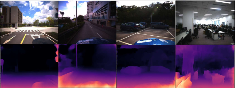
where $d_{est}$ is the estimated depth value at the pixel $\mathbf{x}$ with the corresponding GT depth $d_{gt}$ and where $\delta_{thr}\in\{1.25,1.25^{2},1.25^{3}\}$. Quantitative and some qualitative results are presented in Fig. 17 and Table 7, respectively. These results not only validate our dataset for depth estimation but also highlight the limitations of current unsupervised depth prediction techniques. These limitations are revealed as the FSNet-Handheld model struggles with generalization to handheld sequences, despite training on data with similar appearance. The challenge for monocular depth estimation is further amplified by the significant scale variation in indoor sequences. Advancements in depth formulation and learning strategies are expected to markedly improve the performance in future benchmarks. For a more detailed and comprehensive analysis, we encourage viewing the dataset videos available on our website.

7.4 Known Issues

Creating a comprehensive dataset spanning multiple platforms, sensors, and scenes is labor-intensive. Despite our efforts to resolve many issues, we acknowledge the presence of several imperfections within the dataset. We detail these common challenges in the subsequent sections and present our technical solutions. We hope this discussion will provide valuable insights and lessons for future researchers.

7.4.1 Calibration:

Achieving the life-long sensor calibration poses significant challenges (Maddern et al., 2017). We try our best to provide the best estimate of calibration parameters. Calibration was performed each time when the data collection platform changed, employing SOTA methods for parameter adjustments, which were also manually verified and fine-tuned. For extrinsic parameters difficult to estimate, such as the relative transformation between specific components, we refer to the CAD model. Efforts were made to reinforce the mechanical structure and minimize external disturbances during the data collection process. Nevertheless, it is acknowledged that high accuracy for specific traversals cannot be assured. Users are encouraged to use our calibration estimates as initial values and explore innovative approaches for long-term extrinsic calibration. To aid in these endeavors, we provide raw calibration data and reports, allowing users to develop their methodologies and consider our estimates as a foundational benchmark.

7.4.2 Synchronization:

Section 3.1.1 presents our hardware synchronization solution that guarantees the IMU, frame cameras, and LiDAR are triggered by the same clock source. However, the timestamp of the ROS message of each sensor data has minor differences since the time of data transmission and decode varies. For vehicle-related sequences, the average relative time latency (ARTL) among stereo frame images is smaller than $20ms$. This is mainly caused by the long connection between the camera and the signal trigger. For other sequences, the ARTL is smaller than $5ms$. Due to the special design of the event cameras, the ARTL between the left event camera and the LiDAR is unstable and sometimes smaller than $15ms$.

7.4.3 Partial Loss of Information:

In the construction of the dataset, real-world challenges have led to partial loss of sensor information in certain sequences, reflecting practical issues encountered during robotic deployment. Specifically, for two sequences captured using the Unmanned Ground Vehicle (UGV), the wheel encoder driver was not activated correctly, resulting in the absence of wheel encoder data. Additionally, one sequence from the legged robot experienced brief interruptions in data transmission, amounting to several seconds of lost data, due to a faulty RJ45 network port connection. These instances underscore the importance of robustness in algorithm development to handle incomplete or missing sensor data in realistic operational conditions.

7.4.4 Camera Exposure Setting:

To ensure image consistency during the whole sequence, we fixed the camera exposure time with a specific value before collecting each sequence, mitigating color varies from illumination changes. This scheme is also important to stereo matching since consistent brightness is commonly desirable. However, this scheme can darken images in significantly different lighting conditions, such as entering a tunnel. The darker appearance can be a challenge for most visual perception algorithms.

7.4.5 Scale Discrepancy:

We recognize that the notable limitation of the proposed dataset is the scale, as compared with vast datasets that are trained by exiting foundation models (Brohan et al., 2023). This disparity in scale poses challenges for training robust, generalized SLAM models. Nonetheless, this paper marks a significant initial endeavor in addressing basic challenges in data collection for field robots, including system integration and data postprocessing. This will lay the groundwork for future explorations and expansions in this field.

8 Conclusion and Future Work

In this paper, we present the FusionPortableV2 dataset, a comprehensive multi-sensor collection designed to advance research in SLAM and mobile robot navigation. The dataset is built around a compact, multi-sensor device that integrates IMUs, stereo cameras (both frame- and event-based), LiDAR, and GNSS, all of which are carefully calibrated and synchronized. This primary device is deployed on various platforms, including legged robot, low-speed UGV, and high-speed vehicle, each equipped with additional platform-specific sensors such as wheel encoders and legged sensors. Furthermore, the FusionPortableV2 dataset lies in its diverse range of environments, spanning indoor spaces, grasslands, campuses, parking lots, tunnels, downhill roads, and highways. This environmental diversity allows the dataset to challenge existing SLAM and navigation technologies with realistic scenarios that involve dynamic objects and variable lighting conditions. To ensure the dataset’s utility for the research community, we have meticulously designed $27$ sequences, totaling $2.5$ hours of data, and have provided GT data for objective evaluation of SOTA methods in localization, mapping, and monocular depth estimation.

As we explore future directions for this work, we aim to enhance this dataset’s applicability beyond SLAM, by developing novel navigation methods based on the proposed dataset. We continue to improve the quality of the data and integration of the system for easier manufacture by nonexpert users. Alongside this dataset, we release our implementation details and tools to encourage further research advancements.

This research greatly benefited from the guidance and expertise of many contributors. We extend our profound gratitude to colleagues: Ruoyu Geng, Lu Gan, Bowen Yang, Tianshuai Hu, Mingkai Jia, Mingkai Tang, Yuanhang Li, Shuyang Zhang, Bonan Liu, Jinhao He, Ren Xin, Yingbing Chen, etc. from HKUST and HKUSTGZ for significantly improving our dataset’s quality and applicability, especially in data collection. Special acknowledgment goes to the BIM Lab at HKUST, particularly Prof. Jack Chin Pang Cheng and his students, for their crucial BLK360 scanning expertise and insights that were essential in shaping our dataset. The authors also gratefully acknowledge Dr. Thien-Minh Nguyen (NTU) and Ms. Qingwen Zhang (KTH) for their insightful feedback and technical support; Prof. Dimitrios Kanoulas (UCL), Prof. Martin Magnusson (Örebro University), Prof. Hong Zhang (Southern University of Science and Technology), and Prof. Peng Yin (CityU Hong Kong) for their invaluable dataset writing advice; Mr. Seth G. Isaacson (University of Michigan) for his suggestions on dataset structure. The author(s) received no financial support for the research, authorship, and/or publication of this article.

The authors declared no potential conflicts of interest with respect to the research, authorship, and/or publication of this article.

References

- Agarwal et al. (2020) Agarwal S, Vora A, Pandey G, Williams W, Kourous H and McBride J (2020) Ford multi-av seasonal dataset. The International Journal of Robotics Research 39(12): 1367–1376.
- Barnes et al. (2020) Barnes D, Gadd M, Murcutt P, Newman P and Posner I (2020) The oxford radar robotcar dataset: A radar extension to the oxford robotcar dataset. In: 2020 IEEE International Conference on Robotics and Automation (ICRA). IEEE, pp. 6433–6438.
- Brohan et al. (2023) Brohan A, Brown N, Carbajal J, Chebotar Y, Chen X, Choromanski K, Ding T, Driess D, Dubey A, Finn C et al. (2023) Rt-2: Vision-language-action models transfer web knowledge to robotic control. arXiv preprint arXiv:2307.15818 .
- Brohan et al. (2022) Brohan A, Brown N, Carbajal J, Chebotar Y, Dabis J, Finn C, Gopalakrishnan K, Hausman K, Herzog A, Hsu J et al. (2022) Rt-1: Robotics transformer for real-world control at scale. arXiv preprint arXiv:2212.06817 .
- Burnett et al. (2023) Burnett K, Yoon DJ, Wu Y, Li AZ, Zhang H, Lu S, Qian J, Tseng WK, Lambert A, Leung KY et al. (2023) Boreas: A multi-season autonomous driving dataset. The International Journal of Robotics Research 42(1-2): 33–42.
- Burri et al. (2016) Burri M, Nikolic J, Gohl P, Schneider T, Rehder J, Omari S, Achtelik MW and Siegwart R (2016) The euroc micro aerial vehicle datasets. The International Journal of Robotics Research 35(10): 1157–1163.
- Carlevaris-Bianco et al. (2016) Carlevaris-Bianco N, Ushani AK and Eustice RM (2016) University of michigan north campus long-term vision and lidar dataset. The International Journal of Robotics Research 35(9): 1023–1035.
- Chaney et al. (2023) Chaney K, Cladera F, Wang Z, Bisulco A, Hsieh MA, Korpela C, Kumar V, Taylor CJ and Daniilidis K (2023) M3ed: Multi-robot, multi-sensor, multi-environment event dataset. In: Proceedings of the IEEE/CVF Conference on Computer Vision and Pattern Recognition Workshops. pp. 4015–4022.
- Delmerico et al. (2019) Delmerico J, Cieslewski T, Rebecq H, Faessler M and Scaramuzza D (2019) Are we ready for autonomous drone racing? the uzh-fpv drone racing dataset. In: 2019 International Conference on Robotics and Automation (ICRA). IEEE, pp. 6713–6719.
- Eigen et al. (2014) Eigen D, Puhrsch C and Fergus R (2014) Depth map prediction from a single image using a multi-scale deep network. Advances in neural information processing systems 27.
- Furgale et al. (2013) Furgale P, Rehder J and Siegwart R (2013) Unified temporal and spatial calibration for multi-sensor systems. In: 2013 IEEE/RSJ International Conference on Intelligent Robots and Systems. IEEE, pp. 1280–1286.
- Furrer et al. (2018) Furrer F, Fehr M, Novkovic T, Sommer H, Gilitschenski I and Siegwart R (2018) Evaluation of combined time-offset estimation and hand-eye calibration on robotic datasets. In: Field and Service Robotics. Springer, pp. 145–159.
- Gadd et al. (2024) Gadd M, De Martini D, Bartlett O, Murcutt P, Towlson M, Widojo M, Muşat V, Robinson L, Panagiotaki E, Pramatarov G et al. (2024) Oord: The oxford offroad radar dataset. arXiv preprint arXiv:2403.02845 .
- Gao et al. (2022) Gao L, Liang Y, Yang J, Wu S, Wang C, Chen J and Kneip L (2022) Vector: A versatile event-centric benchmark for multi-sensor slam. IEEE Robotics and Automation Letters 7(3): 8217–8224.
- Gehrig et al. (2021) Gehrig M, Aarents W, Gehrig D and Scaramuzza D (2021) Dsec: A stereo event camera dataset for driving scenarios. IEEE Robotics and Automation Letters 6(3): 4947–4954.
- Geiger et al. (2013) Geiger A, Lenz P, Stiller C and Urtasun R (2013) Vision meets robotics: The kitti dataset. The International Journal of Robotics Research 32(11): 1231–1237.
- Hu et al. (2024) Hu X, Zheng L, Wu J, Geng R, Yu Y, Wei H, Tang X, Wang L, Jiao J and Liu M (2024) Paloc: Advancing slam benchmarking with prior-assisted 6-dof trajectory generation and uncertainty estimation. IEEE/ASME Transactions on Mechatronics .
- Huang et al. (2010) Huang AS, Antone M, Olson E, Fletcher L, Moore D, Teller S and Leonard J (2010) A high-rate, heterogeneous data set from the darpa urban challenge. The International Journal of Robotics Research 29(13): 1595–1601.
- Jeong et al. (2019) Jeong J, Cho Y, Shin YS, Roh H and Kim A (2019) Complex urban dataset with multi-level sensors from highly diverse urban environments. The International Journal of Robotics Research 38(6): 642–657.
- Jiao et al. (2023) Jiao J, Chen F, Wei H, Wu J and Liu M (2023) Lce-calib: Automatic lidar-frame/event camera extrinsic calibration with a globally optimal solution. IEEE/ASME Transactions on Mechatronics .
- Jiao et al. (2022) Jiao J, Wei H, Hu T, Hu X, Zhu Y, He Z, Wu J, Yu J, Xie X, Huang H et al. (2022) Fusionportable: A multi-sensor campus-scene dataset for evaluation of localization and mapping accuracy on diverse platforms. In: 2022 IEEE/RSJ International Conference on Intelligent Robots and Systems (IROS). IEEE, pp. 3851–3856.
- Khazatsky et al. (2024) Khazatsky A, Pertsch K, Nair S, Balakrishna A, Dasari S, Karamcheti S, Nasiriany S, Srirama MK, Chen LY, Ellis K et al. (2024) Droid: A large-scale in-the-wild robot manipulation dataset. arXiv preprint arXiv:2403.12945 .
- Knights et al. (2023) Knights J, Vidanapathirana K, Ramezani M, Sridharan S, Fookes C and Moghadam P (2023) Wild-places: A large-scale dataset for lidar place recognition in unstructured natural environments. In: 2023 IEEE international conference on robotics and automation (ICRA). IEEE, pp. 11322–11328.
- Lai et al. (2022) Lai H, Yin P and Scherer S (2022) Adafusion: Visual-lidar fusion with adaptive weights for place recognition. IEEE Robotics and Automation Letters 7(4): 12038–12045.
- Li et al. (2024) Li H, Zou Y, Chen N, Lin J, Liu X, Xu W, Zheng C, Li R, He D, Kong F et al. (2024) Mars-lvig dataset: A multi-sensor aerial robots slam dataset for lidar-visual-inertial-gnss fusion. The International Journal of Robotics Research : 02783649241227968.
- Lin and Zhang (2022) Lin J and Zhang F (2022) R3live: A robust, real-time, rgb-colored, lidar-inertial-visual tightly-coupled state estimation and mapping package. In: 2022 International Conference on Robotics and Automation (ICRA). IEEE, pp. 10672–10678.
- Liu et al. (2021) Liu T, hai Liao Q, Gan L, Ma F, Cheng J, Xie X, Wang Z, Chen Y, Zhu Y, Zhang S et al. (2021) The role of the hercules autonomous vehicle during the covid-19 pandemic: An autonomous logistic vehicle for contactless goods transportation. IEEE Robotics & Automation Magazine 28(1): 48–58.
- Liu et al. (2023) Liu Y, Xu Z, Huang H, Wang L and Liu M (2023) Fsnet: Redesign self-supervised monodepth for full-scale depth prediction for autonomous driving. IEEE Transactions on Automation Science and Engineering : 1–1110.1109/TASE.2023.3290348.
- Lowry et al. (2015) Lowry S, Sünderhauf N, Newman P, Leonard JJ, Cox D, Corke P and Milford MJ (2015) Visual place recognition: A survey. ieee transactions on robotics 32(1): 1–19.
- Maddern et al. (2017) Maddern W, Pascoe G, Linegar C and Newman P (2017) 1 year, 1000 km: The oxford robotcar dataset. The International Journal of Robotics Research 36(1): 3–15.
- Majdik et al. (2017) Majdik AL, Till C and Scaramuzza D (2017) The zurich urban micro aerial vehicle dataset. The International Journal of Robotics Research 36(3): 269–273.
- Matsuki et al. (2023) Matsuki H, Murai R, Kelly PH and Davison AJ (2023) Gaussian splatting slam. arXiv preprint arXiv:2312.06741 .
- Mescheder et al. (2019) Mescheder L, Oechsle M, Niemeyer M, Nowozin S and Geiger A (2019) Occupancy networks: Learning 3d reconstruction in function space. In: Proceedings of the IEEE/CVF conference on computer vision and pattern recognition. pp. 4460–4470.
- Miller et al. (2018) Miller M, Chung SJ and Hutchinson S (2018) The visual–inertial canoe dataset. The International Journal of Robotics Research 37(1): 13–20.
- Mueggler et al. (2017) Mueggler E, Rebecq H, Gallego G, Delbruck T and Scaramuzza D (2017) The event-camera dataset and simulator: Event-based data for pose estimation, visual odometry, and slam. The International Journal of Robotics Research 36(2): 142–149.
- Nguyen et al. (2022) Nguyen TM, Yuan S, Cao M, Lyu Y, Nguyen TH and Xie L (2022) Ntu viral: A visual-inertial-ranging-lidar dataset, from an aerial vehicle viewpoint. The International Journal of Robotics Research 41(3): 270–280.
- Oquab et al. (2023) Oquab M, Darcet T, Moutakanni T, Vo H, Szafraniec M, Khalidov V, Fernandez P, Haziza D, Massa F, El-Nouby A et al. (2023) Dinov2: Learning robust visual features without supervision. arXiv preprint arXiv:2304.07193 .
- Padalkar et al. (2023) Padalkar A, Pooley A, Jain A, Bewley A, Herzog A, Irpan A, Khazatsky A, Rai A, Singh A, Brohan A et al. (2023) Open x-embodiment: Robotic learning datasets and rt-x models. arXiv preprint arXiv:2310.08864 .
- Pan et al. (2022) Pan Y, Kompis Y, Bartolomei L, Mascaro R, Stachniss C and Chli M (2022) Voxfield: Non-projective signed distance fields for online planning and 3d reconstruction. In: 2022 IEEE/RSJ International Conference on Intelligent Robots and Systems (IROS). IEEE, pp. 5331–5338.
- Pan et al. (2024) Pan Y, Zhong X, Wiesmann L, Posewsky T, Behley J and Stachniss C (2024) Pin-slam: Lidar slam using a point-based implicit neural representation for achieving global map consistency. arXiv preprint arXiv:2401.09101 .
- Pfrommer et al. (2017) Pfrommer B, Sanket N, Daniilidis K and Cleveland J (2017) Penncosyvio: A challenging visual inertial odometry benchmark. In: 2017 IEEE International Conference on Robotics and Automation (ICRA). IEEE, pp. 3847–3854.
- Pire et al. (2019) Pire T, Mujica M, Civera J and Kofman E (2019) The rosario dataset: Multisensor data for localization and mapping in agricultural environments. The International Journal of Robotics Research 38(6): 633–641.
- Qin et al. (2018) Qin T, Li P and Shen S (2018) Vins-mono: A robust and versatile monocular visual-inertial state estimator. IEEE Transactions on Robotics 34(4): 1004–1020.
- Ramezani et al. (2020) Ramezani M, Wang Y, Camurri M, Wisth D, Mattamala M and Fallon M (2020) The newer college dataset: Handheld lidar, inertial and vision with ground truth. In: 2020 IEEE/RSJ International Conference on Intelligent Robots and Systems (IROS). IEEE, pp. 4353–4360.
- Rehder et al. (2016) Rehder J, Nikolic J, Schneider T, Hinzmann T and Siegwart R (2016) Extending kalibr: Calibrating the extrinsics of multiple imus and of individual axes. In: 2016 IEEE International Conference on Robotics and Automation (ICRA). IEEE, pp. 4304–4311.
- Reinke et al. (2022) Reinke A, Palieri M, Morrell B, Chang Y, Ebadi K, Carlone L and Agha-Mohammadi AA (2022) Locus 2.0: Robust and computationally efficient lidar odometry for real-time 3d mapping. IEEE Robotics and Automation Letters 7(4): 9043–9050.
- Schubert et al. (2018) Schubert D, Goll T, Demmel N, Usenko V, Stückler J and Cremers D (2018) The tum vi benchmark for evaluating visual-inertial odometry. In: 2018 IEEE/RSJ International Conference on Intelligent Robots and Systems (IROS). IEEE, pp. 1680–1687.
- Shah et al. (2023a) Shah D, Sridhar A, Bhorkar A, Hirose N and Levine S (2023a) Gnm: A general navigation model to drive any robot. In: 2023 IEEE International Conference on Robotics and Automation (ICRA). IEEE, pp. 7226–7233.
- Shah et al. (2023b) Shah D, Sridhar A, Dashora N, Stachowicz K, Black K, Hirose N and Levine S (2023b) Vint: A foundation model for visual navigation. arXiv preprint arXiv:2306.14846 .
- Teed and Deng (2021) Teed Z and Deng J (2021) Droid-slam: Deep visual slam for monocular, stereo, and rgb-d cameras. Advances in neural information processing systems 34: 16558–16569.
- Wang et al. (2020) Wang W, Zhu D, Wang X, Hu Y, Qiu Y, Wang C, Hu Y, Kapoor A and Scherer S (2020) Tartanair: A dataset to push the limits of visual slam. In: 2020 IEEE/RSJ International Conference on Intelligent Robots and Systems (IROS). IEEE, pp. 4909–4916.
- Wisth et al. (2022) Wisth D, Camurri M and Fallon M (2022) Vilens: Visual, inertial, lidar, and leg odometry for all-terrain legged robots. IEEE Transactions on Robotics 39(1): 309–326.
- Xu et al. (2022) Xu W, Cai Y, He D, Lin J and Zhang F (2022) Fast-lio2: Fast direct lidar-inertial odometry. IEEE Transactions on Robotics 38(4): 2053–2073.
- Yang et al. (2023) Yang S, Zhang Z, Fu Z and Manchester Z (2023) Cerberus: Low-drift visual-inertial-leg odometry for agile locomotion. In: 2023 IEEE International Conference on Robotics and Automation (ICRA). IEEE, pp. 4193–4199.
- Yin et al. (2021) Yin J, Li A, Li T, Yu W and Zou D (2021) M2dgr: A multi-sensor and multi-scenario slam dataset for ground robots. IEEE Robotics and Automation Letters 7(2): 2266–2273.
- Yin et al. (2022) Yin P, Zhao S, Ge R, Cisneros I, Fu R, Zhang J, Choset H and Scherer S (2022) Alita: A large-scale incremental dataset for long-term autonomy. arXiv preprint arXiv:2205.10737 .
- Zhang et al. (2022) Zhang L, Helmberger M, Fu LFT, Wisth D, Camurri M, Scaramuzza D and Fallon M (2022) Hilti-oxford dataset: A millimeter-accurate benchmark for simultaneous localization and mapping. IEEE Robotics and Automation Letters 8(1): 408–415.
- Zhang (2000) Zhang Z (2000) A flexible new technique for camera calibration. IEEE Transactions on pattern analysis and machine intelligence 22(11): 1330–1334.
- Zhu et al. (2018) Zhu AZ, Thakur D, Özaslan T, Pfrommer B, Kumar V and Daniilidis K (2018) The multivehicle stereo event camera dataset: An event camera dataset for 3d perception. IEEE Robotics and Automation Letters 3(3): 2032–2039.
- Zuñiga-Noël et al. (2020) Zuñiga-Noël D, Jaenal A, Gomez-Ojeda R and Gonzalez-Jimenez J (2020) The uma-vi dataset: Visual–inertial odometry in low-textured and dynamic illumination environments. The International Journal of Robotics Research 39(9): 1052–1060.