Control of high-dimensional collective dynamics by deep neural feedback laws and kinetic modelling
Giacomo Albia, Sara Bicegob, Dante Kaliseb
a Department of Computer Science, University of Verona, Strada le Grazie 15, Verona, 37134, Italy
b Department of Mathematics, Imperial College London, South Kensington
Campus, London, SW72AZ, UK
Abstract
Modeling and control of agent-based models is twice cursed by the dimensionality of the problem, as both the number of agents and their state space dimension can be large. Even though the computational barrier posed by a large ensemble of agents can be overcome through a mean field formulation of the control problem, the feasibility of its solution is generally guaranteed only for agents operating in low-dimensional spaces. To circumvent the difficulty posed by the high dimensionality of the state space a kinetic model is proposed, requiring the sampling of high-dimensional, two-agent sub-problems, to evolve the agents’ density using a Boltzmann type equation. Such density evolution requires a high-frequency sampling of two-agent optimal control problems, which is efficiently approximated by means of deep neural networks and supervised learning, enabling the fast simulation of high-dimensional, large-scale ensembles of controlled particles. Numerical experiments demonstrate the effectiveness of the proposed approach in the control of consensus and attraction-repulsion dynamics.
1 Introduction
Collective behaviour in agent-based models (ABMs) is of evergrowing across various disciplines, including mathematics, physics, biology, and economics. ABMs enable the description of complex phenomena through a general paradigm that combines endogenous interactions between agents with external influences. Their applicability spans diverse areas , such as social sciences [44, 28], robotics and computer science [21]. A fundamental topic of interest in ABMs is the study of pattern formation and self-organization [52, 8]. However, beyond self-organization, a fascinating topic arises in relation to the design of external signals or controls to influence a system and inducing a prescribed collective behaviour [18].
Agent-based models encode pairwise agent-to-agent interactions through a balance of attraction and repulsion forces acting over first or second-order dynamics, while the influence of the external world on the system is expressed as a suitable control signal. Let us consider a second order system with agents in , where the state of the -th agent is encoded by the pair , representing position and velocity, respectively, evolving according to transport-interaction dynamics of the form
| (1) | ||||
Here, denotes an interaction kernel, while is a control signal influencing agent . The ensemble of control signals is denoted by . The core of the self-organization behaviour of the free dynamics resides in , which can induce clustering, polarization or alignment, among many others. This self-organization behaviour can be modified by the influence of an external control law. In the framework of dynamic optimization, this control is synthesized by minimizing a cost functional which rewards the convergence of the system towards a cooperative goal, e.g. consensus
| (OCP) |
where the first term in the summation is promoting consensus towards the target velocity , while is a convex function penalizing the energy spent by the control .
The solution of the optimal control problem defined by minimizing (OCP) subject to (1) is twice cursed by the dimensionality of the problem: solving the OCP becomes prohibitively expensive for large values of (as in swarm robotics or collective animal behaviour where hundreds or thousands of agents are present), as well as for high-dimensional state spaces (i.e. , as in portfolio optimization). However, borrowing a leaf from statistical mechanics, as the number of agents , the individual-based problem can be approximated by a mean field formulation [27]
| (2) | ||||
| subject to | ||||
where is the probability density of having an agent with state at time , and the mean field interaction force is given by the non-local operator
| (3) |
Even though the formulation (2)-(3) alleviates the curse of dimensionality with respect to , it leads to a PDE-constrained optimization problem over dimensions, which becomes prohibitively expensive already for moderate values of . In order to overcome this second obstacle, in this paper we resort to modeling the evolution of the agents density from a kinetic viewpoint, reformulating the mean field controlled dynamics as a Povzner-Boltzmann type equation
| (4) |
where the operator takes into account the gain and the loss of particles in at time , due to the motion of individuals via free transport and the velocity changes resulting from the controlled interaction dynamics, see [50, 46]. If we consider the interaction dynamics in (1), reduced to the case of particles with velocities , by denoting as the update of those velocities after a forward Euler step of length , we have
| (5) |
where are the pre-interaction velocities that generate the couple , while is the Jacobian of the binary interactions map .
We will show that this alternative mesoscopic description of ABMs is consistent with the solution of the constrained mean field PDE in (2), when assuming high frequency and weak interactions between particles, similarly to the grazing-collision limit in kinetic theory [37]. The convenience of such kinetic formulation relies on the reduced computational cost required for its solution via direct simulation Monte Carlo (DSMC) methods, [4]. Such a sampling-based technique approximates the solution of the mean field OCP (2) by computing a collection of binary sub-problems for couples of agents sampled from the population density function [46].
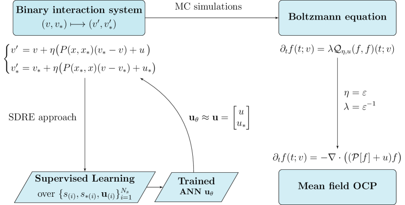
Assuming a high interaction frequency between agents requires, at each evolution step, the solution of a large number of reduced 2-agent OCP associated to (1)-(OCP). For efficiency purposes, we rely on supervised learning to build an Artificial Neural Networks (ANN) approximating the solution of the binary OCP, thus circumventing its online solution at every sampling instance. For training, we generate synthetic data via the solution of the binary OCP by means of a discrete time state-dependent Riccati equation (SDRE) approach [31, 61]. The overall procedure is outlined in Figure 1.
Related literature and contributions
Simulation and control of high-dimensional ABMs is a longstanding and challenging topic. The modeling of such systems has been extensively studied within the kinetic research community, aiming at reducing the computational complexity of simulations [12, 13, 23]. The formulation of a kinetic description for evolutionary models has inspired a flourishing literature in ABMs [15, 47, 56, 57]. In this direction, the authors of [5] proposed a Monte Carlo approach based on binary collision dynamics [46], inspired from plasma physics. The proposed methodology addresses the integration of the mean field formulation of ABMs by means of a Boltzmann scheme, allowing to retrieve the mean field evolution of the system as a limit of 2-agents sub-problems. Such complexity reduction has motivated the extension of this numerical scheme to fit the optimal control framework [4, 48, 49].
In [4, 2], consistency was proven between the solution of mean field OCP and the quasi-invariant limit of controlled binary interaction, where the control action has been optimized by means of model predictive control (MPC) [51], or via dynamic programming (DP) [11]. Similar approaches can be found also in [6] for leader-follower multi-agent systems. In the MPC case, the controller is to be considered sub-optimal, as it is designed to optimize the OCP up to a reduced horizon. DP instead, leads to optimal solutions for the binary OCP, but it requires the solution of a first-order nonlinear Hamilton-Jacobi-Bellman (HJB) PDE cast in the state-space of the system, which can be of arbitrarily high dimension.
Over the last years, the solution of high-dimensional HJB-PDEs has been addressed with a number of different numerical approaches [10, 24, 42, 29, 43], and a flourishing literature on ANNs. ANN methods are differentiated between unsupervised learning techniques [20, 38, 39, 53] and supervised ones [32, 1, 60]. Examples of deep learning algorithms for solving PDEs can be found in [59] for high dimensional Boltzmann equations, or in [35, 54] for more general applications.
The main contributions of our work, inspired by the aforementioned results, can be summarized as follows:
-
•
Aiming at a further reduction in computational complexity with respect to [4, 2], we rely on data-driven approximation models fitted in a supervised learning fashion over synthetic data for the reduced binary OCP. For this, we consider candidate approximation models of both feed-forward (FNN) and recurrent (RNN) neural network type. The architecture of such fitted approximation models conveniently allows for batch evaluations of data, meaning that at each time step the controls can be computed for all the sampled 2-agents sub-systems at once. The precision of the fitted models and their efficiency as the dimensionality of the problem increases have been assessed through numerical tests.
-
•
The dataset guiding the ANNs training phase is collected from synthetic data, obtained from the solution of the infinite horizon OCP (1)-(OCP) reduced to the binary case. Unlike the approaches taken in [2], we circumvent the solution of the HJB equation associated to the binary OCP, which would be unfeasible even in moderate dimensions. Instead, we rely on a procedure for synthesizing nonlinear feedback controls that combines elements from both DP and MPC: the State-Dependent Riccati equation approach. In particular, we will focus on discrete time settings [26, 17].
-
•
A first, intuitive, choice is to consider the feedback control as target variable of the approximation task, as done in [51, 1, 32, 34, 25]. Furthermore, we also train networks for approximating the whole of the controlled right hand side of the discrete-time binary controlled dynamics. For uncontrolled systems, approximation techniques has been studied for detection and approximation of interaction kernels [14, 36]. However, to our knowledge, this work has not been yet extended to the controlled framework.
The rest of the paper has been organized as follows. In Section 2 we formulate the mean field optimal control problem (2) from a kinetic viewpoint. This leads to a Boltzmann description of the dynamics, which is then proven to converge to its mean field counterpart when performing a proper scaling of the frequency and strength of interactions. In Section 3 we discuss how to approximate the evolution of system according to the Boltzmann dynamics for the distribution of agents via Monte Carlo simulation: from the current system configuration, we sample a pool of agents, which are then randomly coupled according to statistics of interaction. The post-interaction agents are then considered, so that their sampling distribution models the updated population density. Following this scheme, the evolution of the system is tracked at discrete times. This requires the computation of the feedback control in discrete-time settings, which is addressed in Section 4 by means of a discrete time state-dependent Riccati Equation approach. In Section 5, we discuss a supervised learning approximation to the solution of the binary OCP. Numerical tests are presented in Section 6.
2 A Boltzmann formulation of the mean field control problem
The accurate modeling of self-organization phenomena and optimal control in ABMs requires a large number of interacting individuals, implying the need for the solution of a very high dimensional optimal control problem, which often comes at a prohibitively expensive computational cost. An alternative way to address this problem is to model instead the distribution function describing the density of individuals having state variable at time . The evolution of can be characterized by a kinetic equation accounting for the motion of individuals undergoing pairwise interactions, as modeled in (8). Thus, the mean field dynamics can be retrieved by suitable scaling of the interactions, also referred as quasi-invariant scaling, or grazing collision limit [46, 58]. In particular, the quasi-invariant limit consists of considering an interaction regime where low intensity interactions occur with high frequency. In this regime, the density is expected to converge pointwise in time to the solution of a mean-field control problem (2).
2.1 Binary controlled dynamics
We denote by the position and velocity states of two agents in the population, and we assume that they modify their velocity states according to binary interaction maps as follows
| (6) | ||||
where is the strength of interaction, is the forcing term associated to interaction between agents. The goal of such external influence is to steer a couple of agents toward consensus. In particular, we will address the optimal control as the solution of an infinite horizon binary optimal control problem, as follows
| (7) |
The numerical procedure for the feedback control synthesis will be addressed in section 4.
Furthermore, we model the evolution in time of with a kinetic integro-differential equation of Boltzmann type [2, 45, 50]
| (8) |
where the parameter encodes the interaction frequency, and the operator accounts for the gain and loss of particles with state at time
| (9) |
In particular, assuming that the binary dynamics (6) preserve the boundary of the bounded set we can express respectively the gain and loss operators as follows
| (10a) | ||||
| (10b) | ||||
where are the pre-interaction velocities that generate the couple , while is the Jacobian of the binary interactions map (6).
2.2 Consistency with the mean field formulation
Here we focus on the consistency of the Boltzmann operator (9) with a mean field controlled dynamics as in (2), in particular introducing a quasi-invariant optimality limit we can regularize such operator, considering a regime where interactions strength is low and frequency is high. This technique, analogous to the grazing collision limit in plasma physics, has been thoroughly studied in [58] and specifically for first order models in [19, 7], and allows to pass from Boltzmann equation (8) to a mean field equation [4, 6]. In what follows we consider the change of notation for the control in the binary dynamics (6)
to give explicit dependence on the parameters and the state variables, since we focus on feedback type controls, and we introduce the following assumptions
-
the system (6) constitutes an invertible changes of variables from to ;
-
there exists an integrable function such that the following limit is well defined
(11)
Hence, in accordance with [15] and with [2], where an analogous of this argument is furnished for the controlled dynamics in stochastic settings, we state the following theorem.
Theorem 2.1
Let us fix the parameters , , and the control , where is the class the admissible controls. Furthermore we assume the kernel function for all , where
Thus, introducing the scaling
| (12) |
for the binary interaction (6) and defining with a solution for the scaled equation (8), for converges pointwise, up to a subsequence, to where satisfies the following mean field equation,
| (13) |
with initial data and where represents the interaction kernel (3) and the control is such that
| (14) |
where is defined as the limiting value in (11).
2.3 Full state controlled binary dynamics
A further generalization can be made introducing a binary interaction dynamics where, differently from the previous section, we consider a binary exchange of information for the full states of the agents . The interacting process defining is described by a binary rules of the following type
| (15) | ||||
where the controls are respectively , and the operators and are defined accordingly to (6) as follows
| (16) |
Thus the kinetic density is solution to the corresponding Boltzmann-type model accounting for the statistical exchange of information of the binary interaction (15) written in the weak form as follows
| (17) |
for a given test function , where, differently to (8), the transport part is embedded into the interaction of the agents. Hence it can be shown that Theorem 2.1 holds also for the latter kinetic model, following the same computation adapted from [2, 45]. Indeed, in the quasi-invariant scaling and , we substitute in the weak formulation the following Taylor’s expansion
| (18) |
Integrating by parts and neglecting the reminder term in the limit we retrieve the weak mean-field model
| (19) |
Thus, recalling that and that the operators are defined as in (16), we retrieve in the strong form the limiting kinetic equation as in (2).
The full state binary interaction (15) will be used, in a reformulated version, to provide the control synthesis for the second-order dynamics.
3 Asymptotic Monte Carlo methods for constrained mean-field dynamics
We provide a fast simulation numerical scheme for the Povzner-Boltzmann-type controlled equation, in the asymptotic regime, reminiscent of Direct Simulaton Monte Carlo methods (DSMCs), used in plasma physics, [13, 12, 5] and later adapted to collective dynamics [5, 55].
First of all, considering a splitting of the transport and collisional term of the Boltzmann-type equation (8) in the asymptotic regime in two different steps [5]:
| (20) |
The purpose of the splitting scheme (20) is to focus the discussion on the convergence of the collisional term, since the free transport process coincides with the mean field formulation and the Boltzmann one.
In the previous section, consistency between the time evolution of the agents’ population has been proven between the mean field model for the population density function, and a scaled Boltzmann description for the dynamics. The latter modeling of is guided by the reduced microscopic binary interactions (6) between agents. This motivates the resorting to Monte Carlo simulation techniques for the approximation of the population density function under the Boltzmann formulation [46, 45, 5, 2].
The evolution (20) of in can be modeled by means of a Forward Euler method, for which we define a time step , and discrete times for
| (21) |
In the spirit of DSMC methods, we can design a stochastic simulation scheme where we sample agents from and we approximate the time variation of as the evolution of the sampled distribution according to the post transport/interaction states.
Concerning the free transport process, the time evolution amounts to the exact free flow at time of sample particles evolving as follows
| (22) |
The collisional term in the Boltzmann-type equation (20), can be rewritten in dependence of the gain and loss component of the operator :
| (23) |
where represent the total mass
| (24) |
Assuming to be a probability density function we will consider . The Forward Euler scheme for (23), with the notation reads
| (25) |
since is a probability density, thanks to mass conservation is again probability density function. Moreover, under the restriction , also is also a probability density. Equation (25) can be interpret as follows: an agent with state has probability to avoid collision with other agents in each time interval . When, instead, the collision does happen (event with probability ), the evolution follows the interaction law described by the scaled binary interaction, then a sampled pair of agents at time
evolves according to (6) as follows
| (26) | ||||
In what follows we consider the asymptotic regime where where the binary interactions (26) is equivalent to a Forward Euler scheme for the two agent dynamics, and the particles that interacts at each iteration are maximized according to the scheme (25).
The asymptotic Monte-Carlo algorithm can be formalized in the following procedure
For the generalized binary dynamics (15) an analogous stochastic simulation technique can be designed, where in this case interaction and transport are updated simultaneously considering the particle states at time as follows , .
Up to this moment, the discussion overlooked the derivation of the forcing terms in the interaction (26). These control variable is meant to be of feedback type, as they only depend on the current agents’ states. Nevertheless, the discrete-time nature of the interaction map (26), embeds within the control variable a dependency on the time-step , which in turn is related to the parameter , see for example [2, 4]. In the following section, we address the solution of the discrete time formulation (22)(26) of the binary interaction control problem.
4 Infinite horizon optimal control of binary dynamics
In this section we study the solution of the infinite horizon optimal control problem for the reduced 2-agent system.
We begin by recalling some fundamental notions on optimal control for discrete-time systems [40], to then present its numerical approximation using a discrete-time State-Dependent Riccati Equation approach.
Hence, we reformulate (26) in a general the control-affine discrete time systems of the form:
| (27) |
where and denote the state of the system and the control signal at time , such that
| (28) |
The state-to-state map and the control operator are assumed to be , satisfying and . Note that binary systems of the form (26) fit this setting. Given , and , , we are interested in the infinite horizon optimal control problem
| (29) |
subject to the dynamics (27) with initial state . We look for a solution to (29) in feedback form, that is, an optimal control map which is expressed a function of the state, . The computation of an optimal feedback law follows a dynamic programming argument, for which we define as the optimal cost-to-go departing from :
| (30) |
where satisfies the Bellman equation
| (31) |
From this point onwards, as we work globally in the state space, and are treated indistinctly.
In order to better describe the difficulties related to the solution of this optimal control problem, we first focus on the linear quadratic case, where the optimal solution is computed via the discrete-time linear quadratic regulator (LQR). The optimality of the feedback law is ensured by a direct link between the LQR solution and the dynamic programming one, obtained from equation (31). In non-linear settings, the parallelism between the nonlinear QR and DP is broken, together with the optimality of the solution.
4.1 Discrete-time Linear Quadratic Regulator
The discrete time linear quadratic problem is a particular instance of the optimal control problem (29) when , and . Under these assumptions, we make the ansatz , so that the Bellman equation (31) becomes
| (32) |
Solving the equation above leads to an optimal feedback of the form
| (33) |
where is the unique positive definite solution of the discrete-time algebraic Riccati equation (DARE):
| (34) |
Remark 4.1
Consider a discrete first-order binary system as in (26) with constant interaction kernel , with state , target and . In this case, the optimal control problem (29) reads
| (35) |
| (36) |
This formulation corresponds to a linear-quadratic control problem by setting , and
Similarly as in Theorem 2.1, we are interested in the asymptotic limit for , in which case (34) becomes
| (37) |
Exploiting to the symmetric structure of the two agent interaction, can be reduced to diagonal and off-diagonal components, see e.g. [30, 3], obtaining the following
| (38) |
The limiting optimal feedback law is given by
| (39) |
from where it follows that the individual feedback laws are given by
In the limiting kinetic equation this corresponds to the mean-field control model
| (40) |
Notice that the structure of in (38) implies isotropic action of the control in the - dimensional state space.
4.2 Discrete-time Non-Linear Quadratic Regulator
It is feasible to apply LQ to a linearization of the system (36). However, if we want to compute a law accounting for nonlinearities, then we compromise the convenient connection between the DARE and the Bellman equation. Moreover, the computational cost required for the solution consistently increases.
In order to extend LQ to the nonlinear case, we begin by re-arranging the difference equation (27) in semilinear state-dependent form
| (41) |
where we consider where and . Note that this semi-linearization is not unique for systems of order greater than . In what follows, we further assume pointwise controllability, i.e. the pair is controllable.
Similarly to the LQR design, the feedback control policy can be calculated as
| (42) | ||||
where the argument for the operators denotes dependency of the current state with discrete time scale , and is the solution of a DARE with state-dependent coefficients (DSDRE):
| (43) |
The state dependency of the feedback operator suggests the need for consecutive sequential solutions of (43) at every discrete time along a trajectory. Thus, for high dimensions of the state space , the exact solution of the DSDRE (43) comes at a cumbersome computational cost. Between the several numerical approaches that have been proposed to address this, we cite Taylor series method [9] and interpolation for [31], while we refer the interested reader to [41] for a more exhaustive review. In what follows, we rely on a discrete version of the SDRE approach proposed in [31].
4.3 Discrete-time SDRE approach
We aim at circumventing the computational challenge of solving (43) at each time step, by realizing the DSDRE feedback law in a model predictive control fashion: given the current state of the system, we assume the operator to be a positive definite matrix in , meaning that (43) reduces to its algebraic form (34), where the state dependencies in (43) are neglected by accordingly freezing all the operators at the current configuration. The resulting feedback variable leads to a suboptimal approximation of the controlled trajectory between and , after which the procedure is repeated by freezing the system at the updated state .
The main computational bottleneck still persisting with this approach is the availability of a sufficiently fast solver for (34). Efficiency in retrieving the DARE solution is key in the settings under consideration, since an accurate Monte Carlo approximation for is linked to high-frequency sampling of interacting couples of agents. At each time step, we aim at conveniently approximate the controlled post-interaction states for a large number of paired agents, living in an arbitrarily high dimensional state space . We address this task by means of supervised learning approximation, relying on models within the family of Artificial Neural Networks.
5 Neural networks and supervised learning approximation of feedback laws
The computational method proposed in this paper models the time evolution of the population density according to the Forward Euler scheme (25), where the updated density is to be approximated by the sampling distribution of controlled post-interaction states in a Monte Carlo fashion.
In this section, we provide an efficient approximating feedback map for the controlled binary dynamics via Feedforward and Recurrent Neural Networks (FNN/RNN). We briefly define these architectures and supervised learning framework for training [22]. After that, we will focus on the problem of interest, discussing synthetic data generation for feedback laws.
5.1 Feedforward Neural Networks
An artificial neural network of feedforward type is associated with a directed acyclic graph defining the architecture of the model, with finite set of directed edges and a finite set of vertices (or nodes), which is partitioned in three proper distinguished subsets:
-
•
Set consisting of the input vertices, having only outgoing edges, while receiving input scalars from outside the network.
-
•
Set containing the output vertices, with only incoming edges. For every network input, these vertices will store the corresponding output value of the model.
-
•
Set of hidden vertices storing intermediate values.
Vertices are associated with a non-linear activation function and a bias , whilst for every edge there is a weight . The weights and biases are the trainable parameters of the network, and they define a family of many output functions. At each vertex we place a computational unit (neuron) defined as
| (44) |
where is the output of the neuron at vertex .
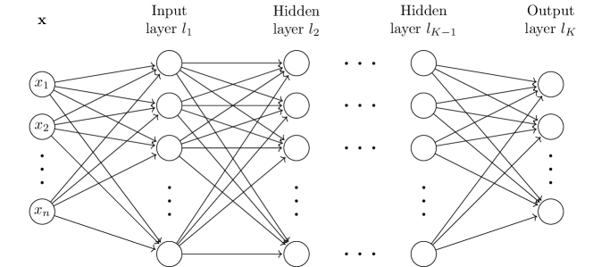
The first class of models we will consider are fully-connected FNNs, where the vertices are organized into layers, and each vertex of every layer is connected via outgoing edges to all vertices in the next one. This family of models is characterized by the flow of information from the input nodes to the output ones without forming any cycles or loops, as shown in Figure 2.
Under the above assumptions, the approximation of the target function via FNNs can be described as , where is defined by a chain of compositions of layer functions
| (45) |
and where
| (46) | |||
with denoting the number of neurons in the -th and -th layer respectively, , and . We define the same activation function for each neuron in the same layer, with the identity function.
In a supervised learning environment, the trainable parameters are then to be computed as minimizers of a suitable loss function measuring the approximation error within a set of sampled data (training set) where :
| (47) |
In particular, we consider
| (48) |
The number of layers , the number of neurons per layer, the set of activation functions in the hidden layers, and eventual other parameters represent further degrees of freedom defining the architecture of the FNN. They are to be computed as result of the hyper-parameter tuning phase, which amounts to choose, between trained models having different architectures, the one performing better w.r.t. some error measure (e.g. the root mean squared error)
| (49) |
where is the validation set such that .
5.2 Recurrent Neural Networks
Recurrent neural networks are a class of models which can be obtained from FNNs by allowing loop connections between layers. This architecture allows particularly good performance when dealing with sequential data. When a sequence is fed as an input, while the output is a single vector, the RNN is said many-to-one; vice versa, a RNN receiving a single input vector and producing a sequence of outputs is called one-to-many. A many-to-many RNN is characterized by input and output of sequential type, while one-to-one RNNs deal with non-sequential data.
Here we extend FNNs into RNNs by allowing hidden layers to be one-to-one Long Short Term Memory (LSTM) cells which – for every input – generate output according to the following system of equations
| (50) |
where the weight matrices and the bias vectors are the trainable parameters, is the activation function, and is the recurrent activation function. The number denotes the number of neurons in the cell. A visual representation of the flux of information through a LSTM cell can be found in Figure 3.
The training and architecture selection for this kind of RNNs consists of the same procedure described in (47) and (49), with the exception that the -th layer is replaced by a LSTM cell, mapping input to output , with parameters .

5.3 Synthetic data generation
Both the training and hyper-parameter tuning phases for the neural network approximation rely on the availability of datasets containing input data points coupled with the corresponding target function evaluations. Since our goal is to approximate the feedback law for the reduced binary controlled dynamics, our target function is the solution of the discrete-time binary optimal control problem, which we address using the discrete-time SDRE approach.
The difference equations for the binary system at the discrete time hold as follows:
| (51) | ||||
being the states for a couple of interacting agents. We introduce the notation , , for which the difference equation reads as in (27)
| (52) |
for and , with and defined as is (16). From this, comes the -dependency of the feedback law : the DSDRE parameters are dependent of the time-step, as will be the DARE solution associated to the system frozen at the current configuration. Therefore, the datasets for the supervised learning approximation of the feedback law, will be generated as samples of pre-interaction states and controls
| (53) |
Similarly, we build a supervised learning approximation for the controlled post-interaction binary states . Since the approximation of the post-interactions positions is direct, the neural network model is restricted to post-interaction velocities , that is . The dataset for training reads
| (54) |
Remark
The addition of the time step to the models’ input allows to train the networks at providing accurate approximations even when applied to adaptive time-step integration techniques.
6 Numerical Tests
In this section we will assess the proposed methodology over consensus control problems for two high dimensional (both in and in ) ABMs. We aim at modeling the time evolution of the agents’ distribution via Monte Carlo simulation of the approximated binary post interaction states. In this section we will compare two different approaches: the approximation of the feedback control map , acting in the binary system (51), and the direct approximation of the controlled dynamics . Algorithm 3 [5] summarizes the proposed numerical procedure for the density evolution once an approximated optimal feedback law has been constructed.
When a neural network is built, we replace line in the algorithm with
| (55) |
The assumption of constant time-step can be easily relaxed, as both the approximants and take as input. In the following numerical tests, the NN training has been done via Adam optimizer [33] with a learning rate over batches of samples.
6.1 Test 1: Cucker-Smale model
The first numerical example for testing the proposed methodology is a consensus control problem for non-linear and non-local dynamics governing the evolution of a -agent system. In its reduced binary semilinear formulation (51), the model is written for the state , with an interaction kernel given by
| (56) |
The control variable is here computed as
| (57) |
with , , and target velocity .
As discussed before, the key ingredient of the proposed methodology is a NN approximation of either the control or the (controlled) update of the reduced binary problem. In both cases, the synthetic data have been generated from uniform samples of interacting couples of agents within , together with their associated (sub)optimal DSDRE feedback control for the discrete-time infinite horizon OCP (42) starting from each for the sampled time-step .
Furthermore, we notice that we can write the state penalty term as
| (58) |
for a suitable block matrix defined as
| (59) |
It follows that
| (60) | ||||
Thus, we can write the cost (57) in quadratic form (29) w.r.t. linear operators
| (61) |
Once the problem has been written in semi-linear form, we rely on the DSDRE approach (described in algorithm 2) for the generation of a dataset collecting samples of coupled states, time-steps, associated feedback laws, and controlled state updates. With a ratio of , we designate those samples to form the training set and the validation set respectively.
We test the following architectures:
hidden layers with neurons, and
LSTM cell with neurons, ,
hidden layers with neurons per layer, and
LSTM cell with neurons, ,
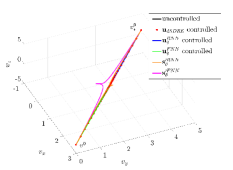
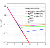
The behaviour of the approximated controlled binary dynamics for a single couple of agents si shown in Figure 4, where we compare the true DSDRE solution with our NN approximations. As the trajectories evolve, the approximated states deviate from the DSDRE closed-loop. However, this does not significantly affect the MC simulation, as a sampled pair of agents will only interact for the duration of a single time step. The goodness of fit of the trained models measured in a test set is presented in Table 3.
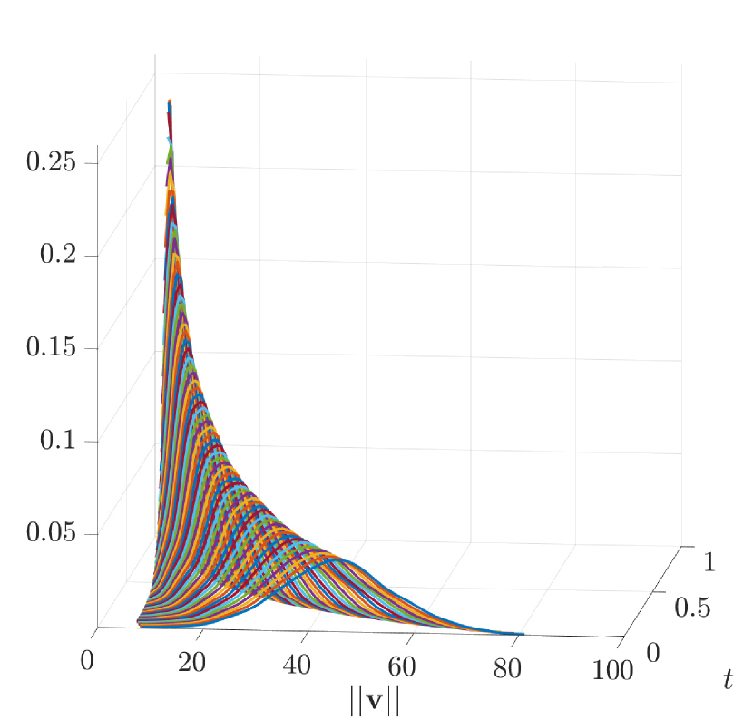
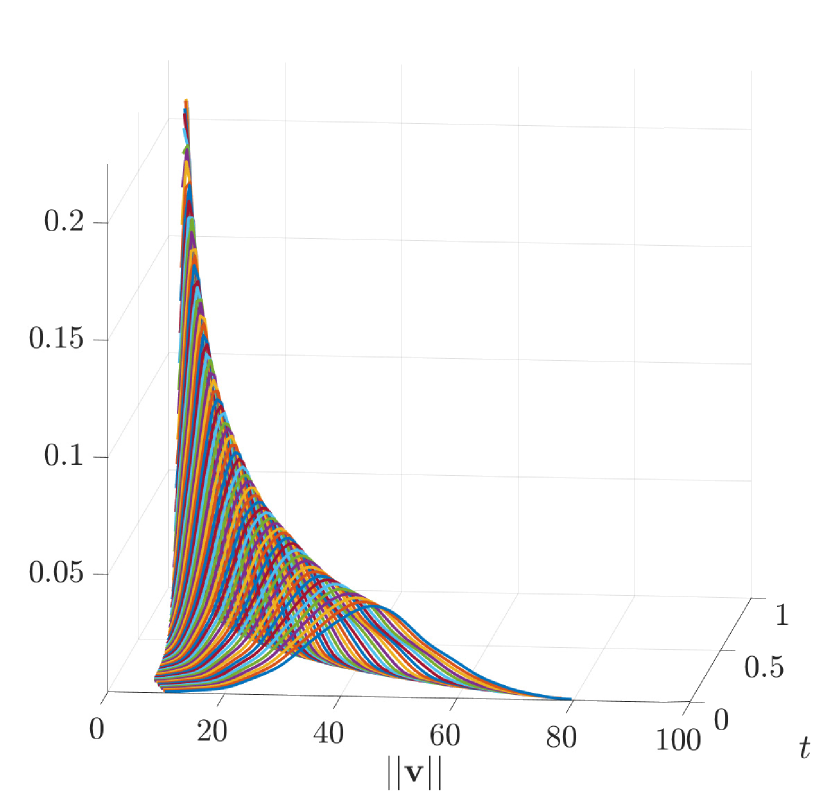
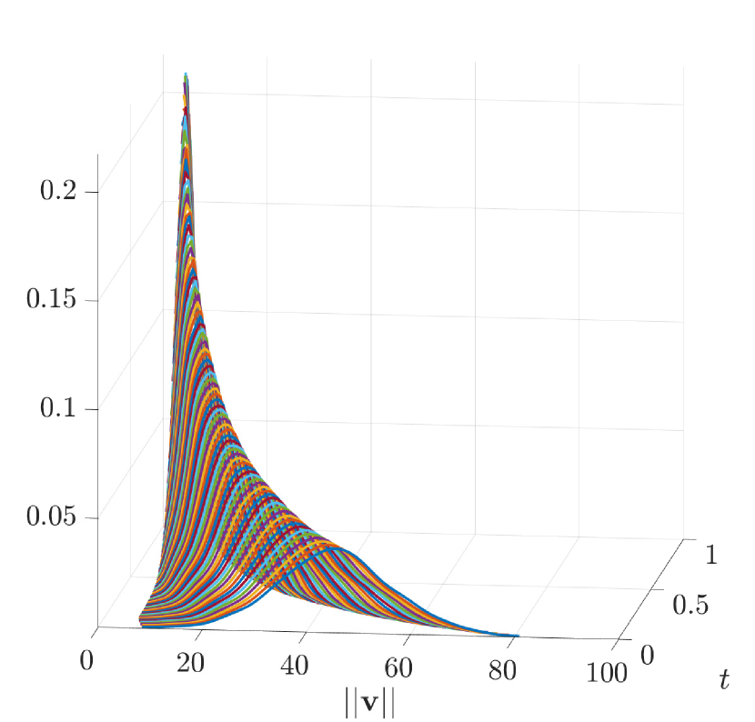
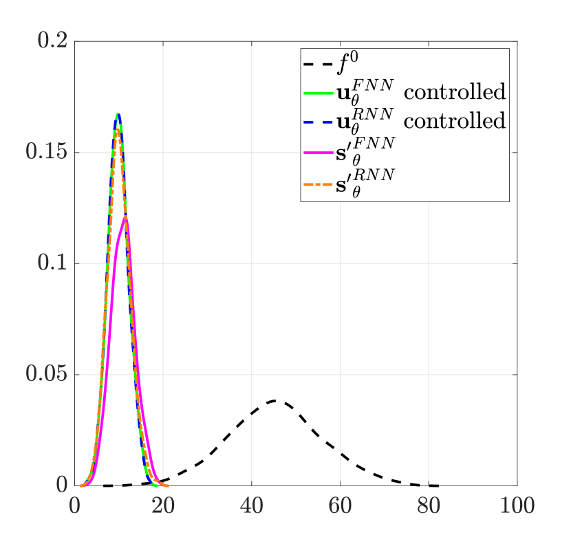
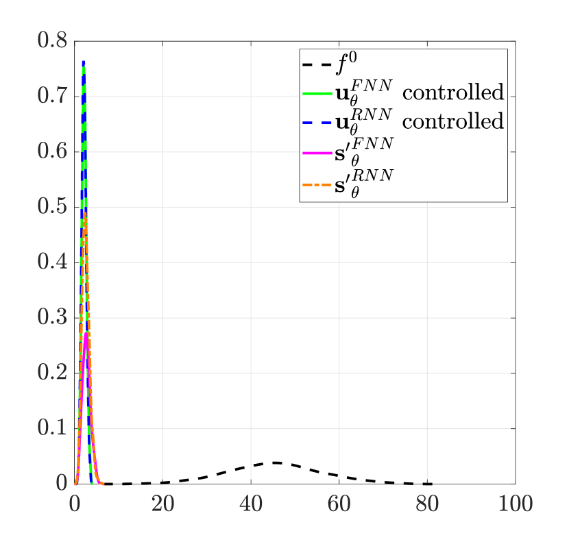
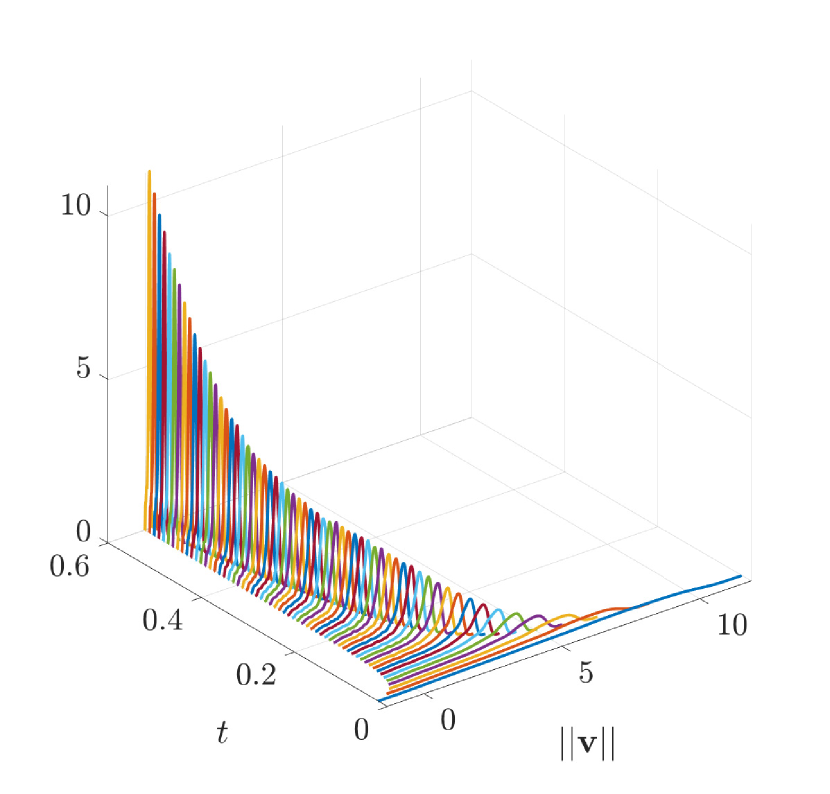
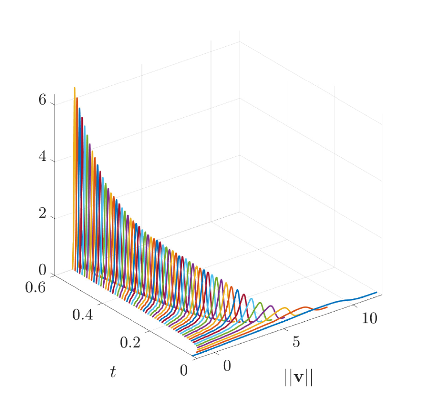
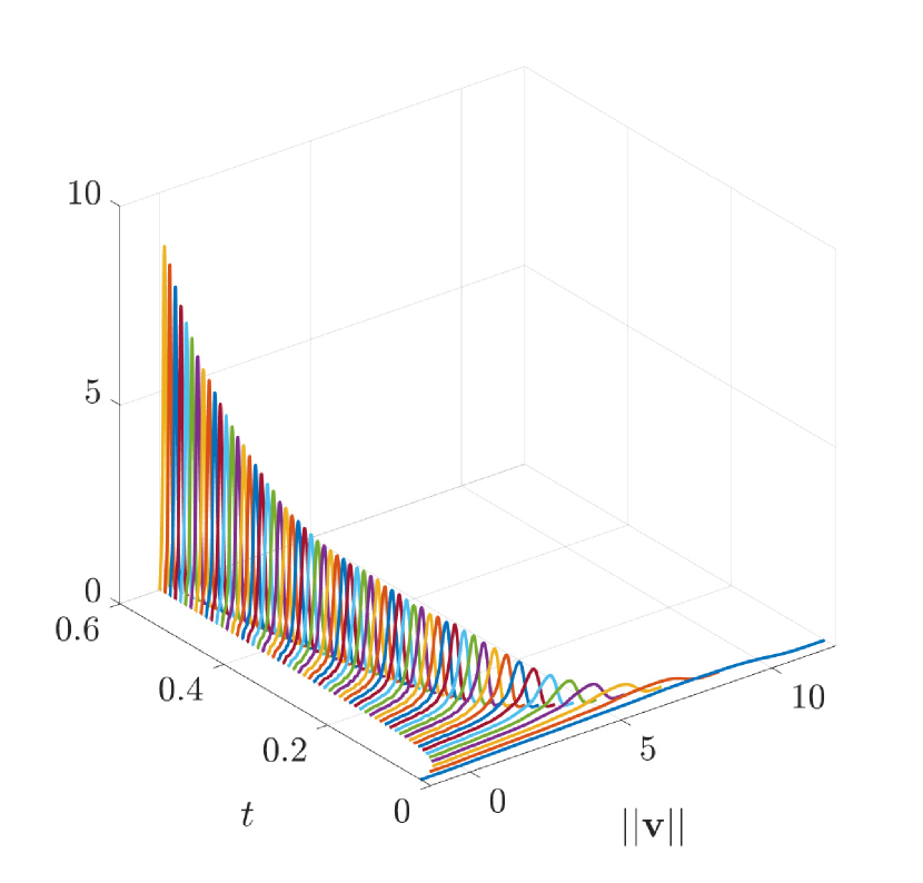
In Figure 5, we show the evolution of the density of agents’ velocities according to a Monte Carlo simulation of binary controlled dynamics, as described in Algorithm 3. All the approximation models equally succeed in steering the density distribution to concentration profiles. Snapshots of the mean field distributions at specific time intervals show how similar the consensus configurations are across the trained models.
So far, the reliance on approximants for the binary controlled state update has been motivated in terms of efficiency. In Tables 1 and 2, we present CPU times111The experiments have been executed in MATLAB R2022a installed on a machine with Intel Core i7-10700 processor running at 2.90GHz. (in seconds) for the MC simulation with the different models, compared with the DSDRE solution . The evolution of the agents’ distribution is approximated along a sequence of discrete times , , . The tables address the computational cost associated to sampling a number of controlled binary interactions in the MC simulation, and the dimensionality of the agents physical space, for a total of dimensions. The reliance on NN approximation models allows for a speedup of to orders of magnitude. For and , the computational cost resulting from the use of displays a linear growth, whilst performs even better. CPU times for the true DSDRE controlled dynamics exceed hours.

| Test 1 | Test 2 | |||||
| Model | MSE | MRE | MSE | MRE | ||
6.2 Test 2: quasi-Morse potential
As a second numerical test, we consider the consensus control problem analysed in [16] for the interacting particles of a second order system of agents in the physical space . The velocities are here governed by both a self-propulsion force, expressed in the agent by the term , for fixed , and an attraction-repulsion force acting though the pairwise interaction potential . We consider a radial potential of the form
| (62) |
with , , , , , in a similar configuration as in [16]. Accordingly, for the couple of interacting agents we define
| (63) |
| (64) |
with which we write the reduced binary dynamics in semilinear form as
| (65) |
where is the diagonal matrices with diagonal vector the component-wise application of to the vector with repetitions of . Moreover, the cost operators for the consensus goal hold as in (61).
As discussed for the previous numerical example, we aim at approximating the binary control , resulting from the DSDRE approach, and the related controlled state update . We train the following models:
hidden layers ( neurons per layer),
( neurons per layer) with LSTM cell,
( neurons per layer),
( neurons per layer), LSTM cell, ,
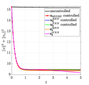
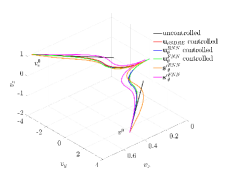
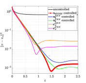
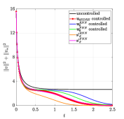
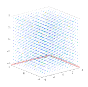
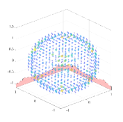
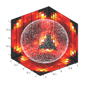
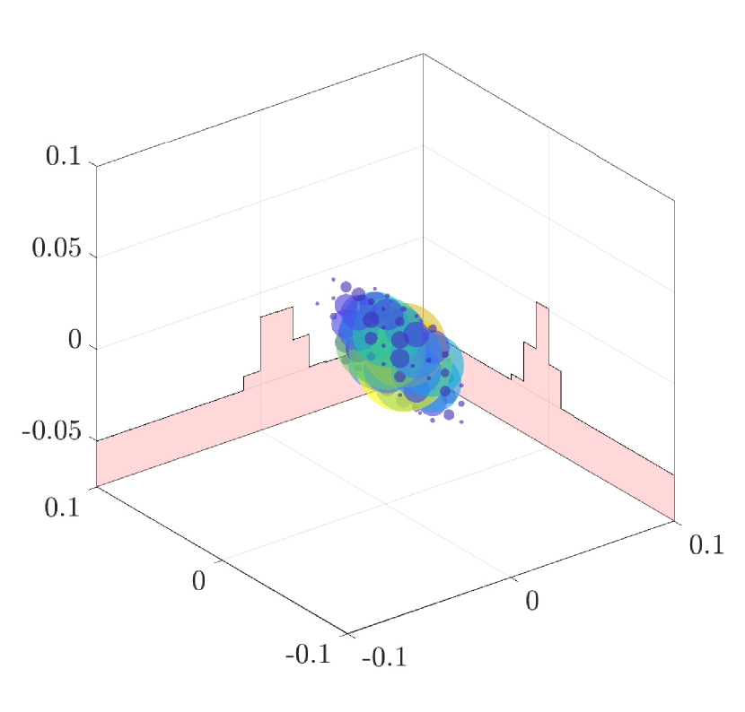
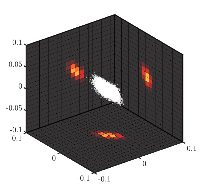
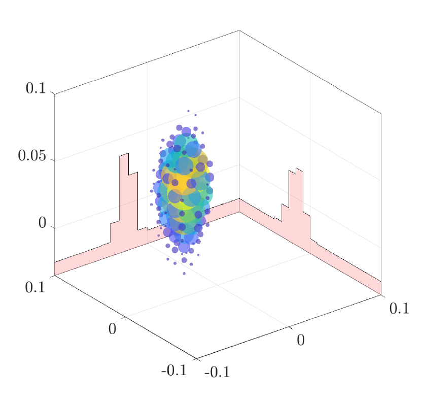
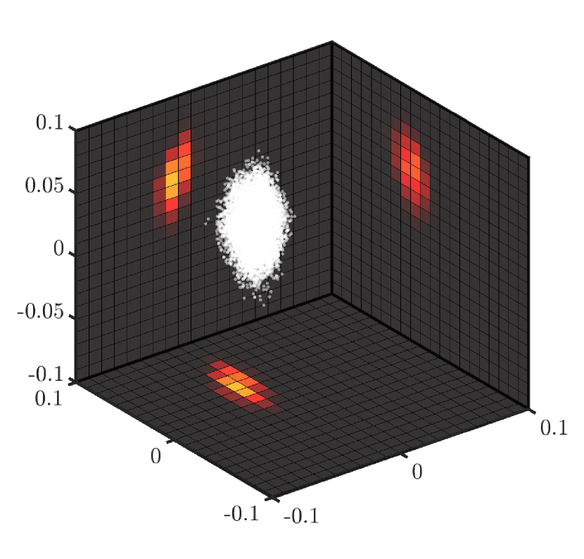
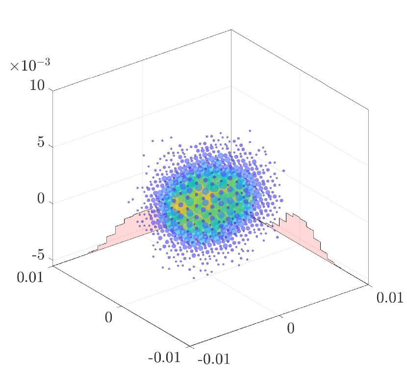
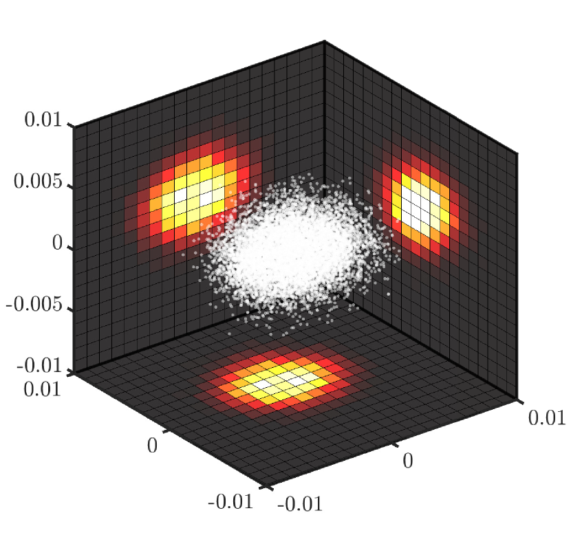
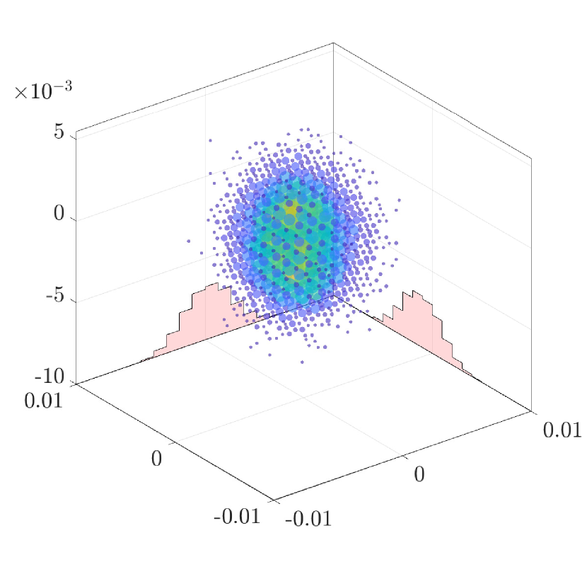
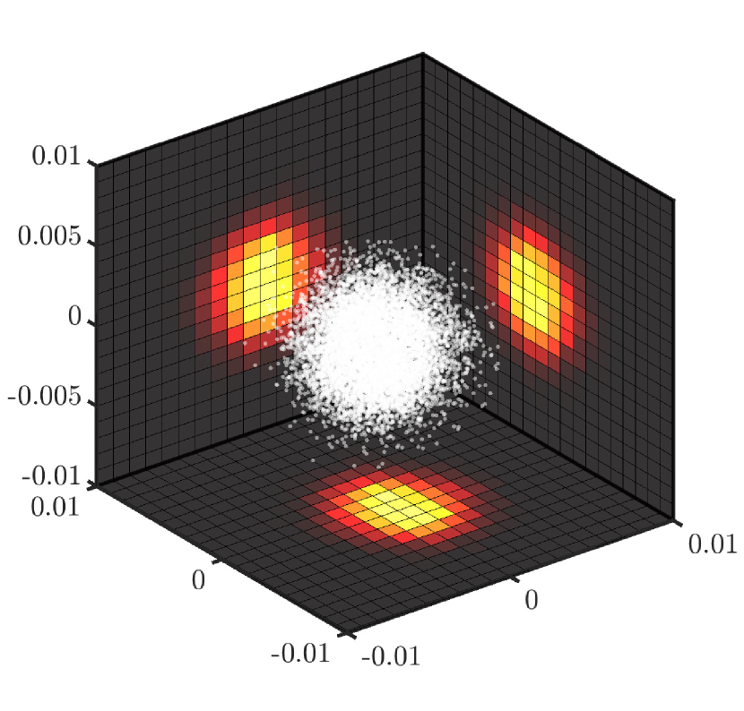
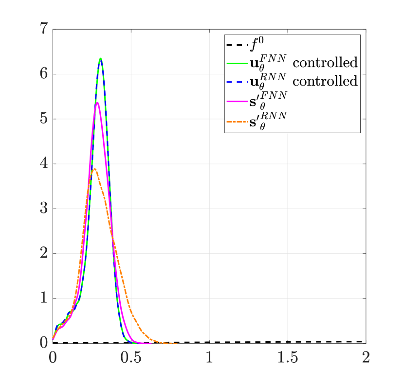
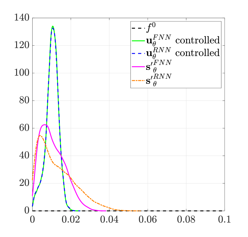
The goodness of fit of these models outside is displayed in table 3, whilst a comparison of the approximately controlled binary system is displayed in Figure 6, where the dynamics of a couple of agents with states randomly sampled in evolve throughout discrete time intervals of length . Whilst all the NN models lead to a similar final state, those approximating the feedback design perform closer to the reference DSDRE solution. As shown in Figure 7, the controlled evolution converges to concentrated density profiles, exhibiting slight differences in mean and variance among the various models. This can also be noticed from the 8, which depicts the density of agents along the first two dimensions, together with the associated vector field of the velocities.

7 Conclusions
We have developed a novel computational method for mitigating the curse of dimensionality arising in the optimal control of large-scale, high-dimensional, agent-based models. The key ingredients of the proposed approach are: the use of a kinetic model to reduce the complexity associated to the particle ensemble to the sampling of two-agent subproblems, and the synthesis of control laws for the two-agent system by means of deep neural networks, supervised learning, and a discrete-time state-dependent Riccati equation approach.
Our numerical experiments validate the effectiveness of the approach in controlling consensus and attraction-repulsion dynamics in high-dimensional interacting particle systems. The use of neural network approximation models for fast feedback synthesis allows for a speedup of 2 to 3 orders of magnitude compared to solving a binary optimal control problem every time two interacting agents are sampled. The proposed framework can be extended to construct a deep neural network that directly predicts the post-interaction states, or to different control problems provided that a solver for synthetic data generator is available.
Potential future research directions include the generalization of the proposed approach to the robust control framework, which could further enhance the applicability of the method to real-world scenarios where robustness to uncertainties in the agents’ interaction forces is crucial. Additionally, exploring the integration of adaptive time-stepping techniques with the neural network approximation models could lead to faster and more accurate simulations of the controlled agent-based system. Finally, investigating the scalability of the proposed approach to even higher-dimensional problems and larger agent populations could enable applications in consensus-based optimization and mean field limits of neural networks.
Acknowledgments
GA thanks the support of MUR-PRIN Project 2022 PNRR No. P2022JC95T, “Data-driven discovery and control of multi-scale interacting artificial agent systems”, and of MUR-PRIN Project 2022 No. 2022N9BM3N “Efficient numerical schemes and optimal control methods for time-dependent partial differential equations” financed by the European Union - Next Generation EU. This research was supported by the UK Engineering and Physical Sciences Research Council (EPSRC) grant EP/T024429/1
Appendix A Proof of Theorem 2.1
Step 1
Let us introduce a test function , where is the state space hosting the agents of the system. We consider the following weak formulation of the Boltzmann equation (8)
| (66) | ||||
Step 2
By definition of the binary post-interaction dynamics (6), we can explicitly write as
| (67) |
where we introduce the function for the controlled dynamics binary dynamics. Moreover, we expand inside the operator (66) in Taylor series of up to the second order, obtaining
| (68) |
where the term represents the reminder of the Taylor expansion as follows
| (69) | ||||
where for some and we use the multi-index notation for the second order partial derivatives of .
Step 3
Embedding (68) into the interacting operator for the weak form (66), and introducing the quasi invariant scaling (12), i.e. , we have
| (70) | ||||
For , assuming that for every the reminder vanishes to zero, then the scaled Boltzmann-type equation (8) in strong form reads
providing a consistency result with the mean-field model (2). Hence, in the next step we show that the reminder is bounded and the previous limit hold true for .
Step 4
Finally we provide estimate on the reminder of the Taylor expansion, to show that such term vanishes for . We observe that
where is the bounding constant of , and since we can conclude that the quasi-invariant limit holds true.
References
- [1] G. Albi, S. Bicego, and D. Kalise. Gradient-augmented supervised learning of optimal feedback laws using state-dependent riccati equations. IEEE Control Systems Letters, 6:836–841, 2022.
- [2] G. Albi, Y.-P. Choi, M. Fornasier, and D. Kalise. Mean field control hierarchy. Appl. Math. Optim., 76(1):93–135, 2017.
- [3] G. Albi, M. Herty, D. Kalise, and C. Segala. Moment-driven predictive control of mean-field collective dynamics. SIAM Journal on Control and Optimization, 60(2):814–841, 2022.
- [4] G. Albi, M. Herty, and L. Pareschi. Kinetic description of optimal control problems and applications to opinion consensus. Commun. Math. Sci., 13(6):1407–1429, 2015.
- [5] G. Albi and L. Pareschi. Binary interaction algorithms for the simulation of flocking and swarming dynamics. Multiscale Modeling & Simulation, 11(1):1–29, 2013.
- [6] G. Albi, L. Pareschi, and M. Zanella. Boltzmann-type control of opinion consensus through leaders. Philosophical Transactions of the Royal Society A: Mathematical, Physical and Engineering Sciences, 372(2028):20140138, 2014.
- [7] G. Aletti, G. Naldi, and G. Toscani. First order continuous models of opinion formation. SIAM Journal on Applied Mathematics, 67:837–853, 2007.
- [8] A. Amirkhani and A. H. Barshooi. Consensus in multi-agent systems: A review. Artif Intell Rev, 55(5), 2022.
- [9] G. C. Andreas Wernli. Suboptimal control for the nonlinear quadratic regulator problem. Automatica, 11(1):75–84, 1975.
- [10] B. Azmi, D. Kalise, and K. Kunisch. Optimal feedback law recovery by gradient-augmented sparse polynomial regression. J. Mach. Learn. Res., 22:Paper No. 48, 32, 2021.
- [11] D. P. Bertsekas. Dynamic programming and optimal control. Vol. I. Athena Scientific, Belmont, MA, fourth edition, 2017.
- [12] G. Bird. Molecular Gas Dynamics and the Direct Simulation of Gas Flows. Number 1 in V. Clarendon Press, 1994.
- [13] A. V. Bobylev and K. Nanbu. Theory of collision algorithms for gases and plasmas based on the Boltzmann equation and the Landau-Fokker-Planck equation. Physical Review E, 61:4576, 4 2000.
- [14] M. Bongini, M. Fornasier, M. Hansen, and M. Maggioni. Inferring interaction rules from observations of evolutive systems I: the variational approach. Math. Models Methods Appl. Sci., 27(5):909–951, 2017.
- [15] J. A. Carrillo, M. Fornasier, J. Rosado, and G. Toscani. Asymptotic flocking dynamics for the kinetic Cucker-Smale model. SIAM J. Math. Anal., 42(1):218–236, 2010.
- [16] J. A. Carrillo, D. Kalise, F. Rossi, and E. Trélat. Controlling Swarms toward Flocks and Mills. SIAM J. Control Optim., 60(3):1863–1891, 2022.
- [17] I. Chang and J. Bentsman. Constrained discrete-time state-dependent Riccati equation technique : A model predictive control approach. Proceedings of the IEEE Conference on Decision and Control, pages 5125–5130, 2013.
- [18] F. Chen and W. Ren. On the control of multi-agent systems: A survey. SYS, 6:339–499, 7 2019. Publisher: Now Publishers, Inc.
- [19] S. Cordier, L. Pareschi, and G. Toscani. On a kinetic model for a simple market economy. Journal of Statistical Physics, 120(1):253–277, 2005.
- [20] J. Darbon, G. P. Langlois, and T. Meng. Overcoming the curse of dimensionality for some Hamilton-Jacobi partial differential equations via neural network architectures. Res. Math. Sci., 7(3):Paper No. 20, 50, 2020.
- [21] Devi, Kskn Venkata Ramana, B S, Smitha, Lakhanpal, Sorabh, Kalra, Ravi, Sethi, Vandana Arora, and Thajil, Sadiq Khader. A review: Swarm robotics: Cooperative control in multi-agent systems. E3S Web Conf., 505:03013, 2024.
- [22] R. DeVore, B. Hanin, and G. Petrova. Neural network approximation. Acta Numerica, 30:327–444, 2021.
- [23] G. Dimarco, Q. Li, L. Pareschi, and B. Yan. Numerical methods for plasma physics in collisional regimes. Journal of Plasma Physics, 81(1):305810106, 2015.
- [24] S. Dolgov, D. Kalise, and K. K. Kunisch. Tensor decomposition methods for high-dimensional Hamilton-Jacobi-Bellman equations. SIAM J. Sci. Comput., 43(3):A1625–A1650, 2021.
- [25] S. Dolgov, D. Kalise, and L. Saluzzi. Data-driven tensor train gradient cross approximation for hamilton-jacobi-bellman equations. SIAM Journal on Scientific Computing, 45(5):A2153–A2184, 2023.
- [26] A. S. Dutka, A. W. Ordys, and M. J. Grimble. Optimized discrete-time state dependent Riccati equation regulator. Proceedings of the 2005, American Control Conference, 4:2293–2298, 2005.
- [27] M. Fornasier and F. Solombrino. Mean-field optimal control. ESAIM Control Optim. Calc. Var., 20(4):1123–1152, 2014.
- [28] B. Geng, S. Brahma, T. Wimalajeewa, P. K. Varshney, and M. Rangaswamy. Prospect theoretic utility based human decision making in multi-agent systems. IEEE Trans. Signal Process., 68:1091–1104, 2020.
- [29] A. Gooran Orimi, S. Effati, and M. H. Farahi. Approximate solution of the Hamilton-Jacobi-Bellman equation. J. Math. Model., 10(1):71–91, 2022.
- [30] M. Herty, L. Pareschi, and S. Steffensen. Mean–field control and Riccati equations. Networks and Heterogeneous Media, 10(3):699–715, 2015.
- [31] H. T. H.T. Banks, B.M. Lewis. Nonlinear feedback controllers and compensators: a state-dependent Riccati equation approach. Computational Optimization and Applications, 37:177–218, 6 2007.
- [32] W. Kang, Q. Gong, T. Nakamura-Zimmerer, and F. Fahroo. Algorithms of data generation for deep learning and feedback design: a survey. Phys. D, 425:Paper No. 132955, 10, 2021.
- [33] D. P. Kingma and J. Ba. Adam: A method for stochastic optimization. CoRR, abs/1412.6980, 2015.
- [34] K. Kunisch and D. Walter. Semiglobal optimal feedback stabilization of autonomous systems via deep neural network approximation. ESAIM Control Optim. Calc. Var., 27:Paper No. 16, 59, 2021.
- [35] I. Lagaris, A. Likas, and D. Fotiadis. Artificial neural networks for solving ordinary and partial differential equations. IEEE Transactions on Neural Networks, 9(5):987–1000, 1998.
- [36] F. Lu, M. Maggioni, and S. Tang. Learning interaction kernels in heterogeneous systems of agents from multiple trajectories. Found Comput Math, 22, 2022.
- [37] S. McNamara and W. R. Young. Kinetics of a one-dimensional granular medium in the quasielastic limit. Phys. Fluids A, 5(1):34–45, 1993.
- [38] Y. Meng, R. Zhou, A. Mukherjee, M. Fitzsimmons, C. Song, and J. Liu. Physics-informed neural network policy iteration: Algorithms, convergence, and verification. arXiv, 2024.
- [39] K.-M. Na and C.-H. Lee. Physics-informed deep learning approach to solve optimal control problem. AIAA SCITECH 2024 Forum, 2024.
- [40] D. S. Naidu and R. C. Dorf. Optimal Control Systems. CRC Press, Inc., USA, 2003.
- [41] S. R. Nekoo. Tutorial and review on the state-dependent Riccati equation. J. Appl. Nonlinear Dyn., 8(2):109–166, 2019.
- [42] M. Oster, L. Sallandt, and R. Schneider. Approximating Optimal feedback Controllers of Finite Horizon Control Problems Using Hierarchical Tensor Formats. SIAM J. Sci. Comput., 44(3):B746–B770, 2022.
- [43] M. Oster, L. Saluzzi, and T. Wenzel. A comparison study of supervised learning techniques for the approximation of high dimensional functions and feedback control. arXiv preprint, 2024.
- [44] Papadopoulou, Furtbauer, O’Bryan, Garnier, Georgopoulou, Bracken, Christensen, and King. Dynamics of collective motion across time and species. Philosophical Transactions of the Royal Society B: Biological Sciences, 378(1874), 2023.
- [45] L. Pareschi and G. Russo. An introduction to Monte Carlo method for the Boltzmann equation. ESAIM: Proceedings, 10:35–75, 2001.
- [46] L. Pareschi and G. Toscani. Interacting multiagent systems. Kinetic equations and Monte Carlo methods. Oxford: Oxford University Press, 2014.
- [47] L. Pareschi and G. Toscani. Wealth distribution and collective knowledge: a Boltzmann approach. Philos. Trans. R. Soc. Lond. Ser. A Math. Phys. Eng. Sci., 372(2028):20130396, 15, 2014.
- [48] L. Pareschi, T. Trimborn, and M. Zanella. Mean-field control variate methods for kinetic equations with uncertainties and applications to socioeconomic sciences. Int. J. Uncertain. Quantif., 12(1):61–84, 2022.
- [49] B. Piccoli, F. Rossi, and E. Trélat. Control to flocking of the kinetic Cucker-Smale model. SIAM J. Math. Anal., 47(6):4685–4719, 2015.
- [50] A. J. Povzner. On the Boltzmann equation in the kinetic theory of gases. Mat. Sb. (N.S.), 58(100):65–86, 1962.
- [51] S. V. Raković and W. S. Levine, editors. Handbook of model predictive control. Control Engineering. Birkhäuser/Springer, Cham, 2019.
- [52] F. Rossi, S. Bandyopadhyay, M. Wolf, and M. Pavone. Review of multi-agent algorithms for collective behavior: a structural taxonomy. IFAC-PapersOnLine, 51(12):112–117, 2018. IFAC Workshop on Networked Autonomous Air Space Systems NAASS 2018.
- [53] L. Ruthotto, S. J. Osher, W. Li, L. Nurbekyan, and S. W. Fung. A machine learning framework for solving high-dimensional mean field game and mean field control problems. Proceedings of the National Academy of Sciences, 117(17):9183–9193, 2020.
- [54] J. Sirignano and K. Spiliopoulos. Dgm: A deep learning algorithm for solving partial differential equations. Journal of Computational Physics, 375:1339–1364, 2018.
- [55] G. Toscani. Kinetic models of opinion formation. Comm. Math. Sci., 4(3):481–496, 2006.
- [56] A. Tosin and M. Zanella. Boltzmann-type models with uncertain binary interactions. Commun. Math. Sci., 16(4):963–985, 2018.
- [57] A. Tosin and M. Zanella. Boltzmann-type description with cutoff of follow-the-leader traffic models. In Trails in kinetic theory—foundational aspects and numerical methods, volume 25 of SEMA SIMAI Springer Ser., pages 227–251. Springer, Cham, [2021] ©2021.
- [58] C. Villani. On a new class of weak solutions to the spatially homogeneous Boltzmann and Landau equations. Archive for rational mechanics and analysis, 143(3):273–307, 1998.
- [59] T. Xiao and M. Frank. Using neural networks to accelerate the solution of the Boltzmann equation. J. Comput. Phys., 443:Paper No. 110521, 22, 2021.
- [60] Y. Zhao and J. Han. Offline supervised learning v.s. online direct policy optimization: A comparative study and a unified training paradigm for neural network-based optimal feedback control. Physica D: Nonlinear Phenomena, 462:134130, 2024.
- [61] T. Çimen. State-dependent Riccati equation (SDRE) control: A survey. IFAC Proceedings Volumes, 41(2):3761–3775, 2008. 17th IFAC World Congress.