Generative-Contrastive Heterogeneous Graph Neural Network

Abstract.

Heterogeneous Graphs (HGs) can effectively model complex relationships in the real world by multi-type nodes and edges. In recent years, inspired by self-supervised learning, contrastive Heterogeneous Graphs Neural Networks (HGNNs) have shown great potential by utilizing data augmentation and discriminators for downstream tasks. However, data augmentation is still limited due to the discrete and abstract nature of graphs. To tackle the above limitations, we propose a novel Generative-Contrastive Heterogeneous Graph Neural Network (GC-HGNN). Specifically, we first propose a heterogeneous graph generative learning enhanced contrastive paradigm. This paradigm includes: 1) A contrastive view augmentation strategy by using masked autoencoder. 2) Position-aware and semantics-aware positive sample sampling strategy for generate hard negative samples. 3) A hierarchical contrastive learning strategy for capturing local and global information. Furthermore, the hierarchical contrastive learning and sampling strategies aim to constitute an enhanced discriminator under the generative-contrastive perspective. Finally, we compare our model with seventeen baselines on eight real-world datasets. Our model outperforms the latest contrastive and generative baselines on node classification and link prediction tasks. To reproduce our work, we have open-sourced our code at https://github.com/xxx.

1. INTRODUCTION

Heterogeneous Information Networks (HIN) or Heterogeneous Graphs (HG) (Sun and Han, 2013; Wang et al., 2019, 2021; Shi et al., 2018; Tian et al., 2023) have become critical tools for analyzing the real world, as they preserve rich semantic information by modeling different types of nodes and edges. This is particularly relevant in networks such as citation networks (Dong et al., 2017; Wang et al., 2019), recommendation systems (Shi et al., 2018; Chen et al., 2023), and social networks (Long et al., 2021). Recently, Heterogeneous Graph Neural Networks (HGNNs) (Wang et al., 2019, 2021; Hu et al., 2020a; Tian et al., 2023) have demonstrated a strong ability in processing HIN data because they have expanded the receptive field of nodes through meta-path (Sun et al., 2011) and message-passing mechanism, thereby capturing the rich semantics.

Figure 1. Heterogeneous graph self-supervised learning with contrastive and generative-contrastive paradigms.

Self-supervised learning has widely applied in the fields of computer vision (CV) (He et al., 2020b; Chen et al., 2020; Grill et al., 2020) and natural language processing (NLP) (Chowdhery et al., 2023; Devlin et al., 2018), leveraging unlabeled data to learn informative representations. Inspired by this trend, researchers begin to explore the combination of HGNNs and self-supervised learning. In particular, contrastive HGNNs (Wang et al., 2021; Zhu et al., 2022; Wang et al., 2023; Chen et al., 2023) have shown great potential because they are more suitable for downstream tasks by discarding the decoder and setting up a discriminator. Data augmentation (Wu et al., 2021; Yang et al., 2023) is crucial for improving the performance of contrastive learning on heterogeneous graphs. However, due to the discrete and abstract nature of graph data, it is difficult to provide reasonable data augmentation to leverage the advantages of contrastive learning (He et al., 2020b; Liu et al., 2021).

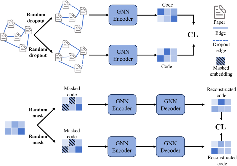
Generative learning (Chowdhery et al., 2023; Tian et al., 2023; Hou et al., 2022; Devlin et al., 2018; Liu et al., 2021) can effectively solve the problem of data augmentation because it can reconstruct the data distribution without considering downstream tasks, allowing the each node embedding to be enhanced. This also provides a foundation for us to propose a generative learning enhanced contrastive paradigm for heterogeneous graphs. As shown in Figure 1, first, HGNNs utilize a meta-path to obtain a graph containing nodes of the same type. Contrastive learning (Wang et al., 2023; Zhu et al., 2022) generates supervised signals by aligning two similar views constructed through random edge dropping; while generative-contrastive learning (Goodfellow et al., 2020; Yang et al., 2023; Wu et al., 2023) generates fake samples by training an autoencoder and uses a discriminator to distinguish them. Despite the obvious advantages of generative-contrastive paradigm, there are still some challenges for heterogeneous graphs:

CH1: Contrastive view challenge. The current augmentation strategies (Wang et al., 2023, 2021; Zhu et al., 2022; Lin et al., 2022; Wu et al., 2021), such as structural and feature augmentation, still have limitations. Structural augmentation (Wang et al., 2023; Zhu et al., 2022; Wu et al., 2021), which involves randomly dropout nodes and edges, could disrupt the graph integrity since nodes and edges are the fundamental properties of a graph. On the other hand, feature augmentation (Wang et al., 2021; Lin et al., 2022), which perturbs node attributes, ignores the unique features of each node’s input. In such methods, some nodes have more edges and embeddings than others, resulting in unbalanced supervised signals. Exploring how to better utilize meta-paths to design enhanced contrastive views remains a challenge that needs to be addressed.

CH2: Sampler challenge. In heterogeneous graphs, contrastive learning (Wang et al., 2023, 2021; Zhu et al., 2022; Chen et al., 2023; Wu et al., 2021) heavy relies on high-quality negative samples. Moreover, the discriminator has stricter requirements for sampling under the generative-contrastive paradigm (Wu et al., 2023). Existing sampling strategies (Wang et al., 2023, 2021; Zhu et al., 2022) are usually based on randomness or meta-paths, which often increase false negative samples. Some recent works (Kalantidis et al., 2020; Liu et al., 2023) aim to select or synthesize hard negatives to mitigate the impact of false negatives. However, they are not suitable for heterogeneous graphs and offer limited benefits. Therefore, designing an enhanced positive sampling strategy for heterogeneous graphs is urgently needed.

CH3: Contrastive mechanism challenge. Existing methods (Wang et al., 2023; Zhu et al., 2022; Tian et al., 2023) rely solely on meta-paths to capture rich semantic information in heterogeneous graphs and often overlook the influence of one-hop neighbors on target nodes. Network schema leverages direct connections between nodes to capture the local structure of target nodes. In contrast, meta-paths extract higher-order structures. Designing an effective self-supervised mechanism that considers both local and global information can better help the model work.

To tackle the three challenges mentioned above, we propose a heterogeneous graph self-supervised model called Generative-Contrastive Heterogeneous Graph Neural Network (GC-HGNN). For CH1, GC-HGNN employs a generative masked autoencoder (MAE) to enhance contrastive views. The MAE can reconstruct node embeddings without altering the original graph structure and features. The masking strategy averages the edges of each node to ensure that each node receives the same supervised signals during the reconstruction process. For CH2, the model proposes a positive sample sampling strategy that combines location-awareness and semantic-awareness. This approach adaptively samples nodes based on the rich semantics unique to heterogeneous graphs and the global positions of nodes in the heterogeneous graph. Finally, for CH3, GC-HGNN utilizes hierarchical contrastive learning to capture one-hop and higher-order neighbors. Intra-contrast is used to contrast different meta-path views, while inter-contrast is used to contrast between network schema and meta-path views. We summarize the contributions of this paper as follows:

• We propose a heterogeneous graph generative learning enhanced contrastive paradigm, leveraging a generative masked autoencoder as a tool for contrastive view augmentation. This represents a meaningful exploration for graph generative adversarial networks.

• We introduce hierarchical contrastive learning as an enhanced discriminator, combined with novel sampling strategies to align with the generative model. All these modules can better mine self-supervised signals under an end-to-end training scenario.

• We conduct comprehensive experiments to evaluate GC-HGNN with seventeen baselines methods and eight real datasets. The experimental results show that GC-HGNN is superior to other methods, and is able to generate enhanced views and effectively extract heterogeneous information.

2. RELATED WORK

This section discusses the development process of heterogeneous graph neural networks. Here, we introduce the issue of infeasible and expensive data labels, further elaborating on the self-supervised advantages and providing a brief overview of existing models.

2.1. Heterogeneous Graph Neural Networks

In recent years, Graph Neural Networks (GNNs) (You et al., 2020; Hu et al., 2020b; Hou et al., 2022; Velickovic et al., 2017; He et al., 2020a) have achieved significant success in fields such as social network analysis and recommender systems. This success relies on their effective modeling of graph structure information and local and global information integration. These graph structures often have different types of nodes and edges. Heterogeneous graph neural networks are designed to better handle heterogeneous graph data.

The currently popular heterogeneous graph neural network models (Wang et al., 2019, 2021; Zhang et al., 2019; Fu et al., 2020; Yu et al., 2022b) can be classified into two categories: meta-path- based methods and types-based methods. The classic meta-path-based models include HAN (Wang et al., 2019), HetGNN (Zhang et al., 2019), and MAGNN (Fu et al., 2020). Specifically, HAN employs a dual-layer attention mechanism at both the node and semantic levels to adaptively capture the relationships between nodes and meta-paths. HetGNN introduces a heterogeneous graph attention propagation mechanism, combining meta-path information and attention mechanisms to learn node representations. MAGNN integrates meta-paths and adaptive mechanisms to learn node representations in heterogeneous graphs by learning meta-path attention weights at both the node and global levels. The type-based models include RGCN (Schlichtkrull et al., 2018), HGT (Hu et al., 2020a), and RHGNN (Yu et al., 2022b). RGCN captures rich semantic relationships by using different weight matrices for different types of edges. HGT achieves efficient representation learning and information propagation on heterogeneous graph data by introducing a multi-head attention mechanism and a heterogeneous graph structure encoder. RHGNN utilizes dedicated graph convolution components and cross-relation message passing modules to learn node representations on heterogeneous graphs. However, the above-mentioned methods only investigate supervised heterogeneous graph models. In order to more deeply explore the potential relationships and patterns in the data, and to effectively utilize unlabeled data, an increasing number of studies are beginning to focus on self-supervised learning methods.

2.2. Self-supervised Graph Learning

With the rapid development of self-supervised learning in computer vision (He et al., 2020b; Chen et al., 2020) and natural language processing (Devlin et al., 2018; Chowdhery et al., 2023) fields, graph neural networks have drawn inspiration from this progress. Self-supervised graph neural networks often train without labels by generating contrastive views or reconstructing node attributes, thus better leveraging the rich structural information in graph data. Transitioning from general graphs to heterogeneous graphs involves assigning different types or attributes to nodes and edges in the graph, making the graph structure more complex and diverse in representation.

Self-supervised heterogeneous graph neural networks can be categorized into: contrastive and generative. Contrastive learning models (Ren et al., 2019; Wang et al., 2021, 2023) generate enhanced contrastive views and attempt to maximize the mutual information between these views to produce supervised signals. Specifically, HDGI (Ren et al., 2019) utilizes graph convolutional modules and semantic-level attention to learn node representations and maximize local-global mutual information. HeCo (Wang et al., 2021) complements across perspectives through network schema and meta-path views, establishing a sampling contrast method between the two views to achieve self-supervised enhancement. HGCML (Wang et al., 2023) solely utilizes the rich semantic relationships brought by meta-paths for graph enhancement, introducing multi-view contrastive learning. It also proposes sampling strategies for positive samples in both topology and semantics to alleviate sampling bias. Generative models (Zheng et al., 2021; Tian et al., 2023) commonly adopt graph autoencoder and attempt to reconstruct features to obtain supervision. For example, MvDGAE (Zheng et al., 2021) utilizes random edge dropout to enhance views and utilizes autoencoders to enforce the recovery of views for more robust representations. Meanwhile, HGMAE (Tian et al., 2023) further introduces dynamic masking mechanism and position-aware encoding to enhance the model’s performance and utilizes attribute and view dual-recovery to improve denoising capability.

Figure 2. A toy example of an HIN on ACM (Wang et al., 2019) dataset.

3. PRELIMINARIES

In this section, we formally define some significant concepts related to HIN as follows:

Heterogeneous Information Network (HIN): A HIN is characterized by a graph structure $G=(V,E,I,J,\phi,\varphi)$, in which the collections of nodes and edges are symbolized by $V$ and $E$ respectively. For every node $v$ and edge $e$, there are associated type mapping functions $\phi:V\rightarrow I$ for nodes and $\varphi:E\rightarrow J$ for edges. Here, $I$ represents the node types and $J$ denotes the edge types, with the total number of types exceeding two, i.e., $|I|+|J|>2$.

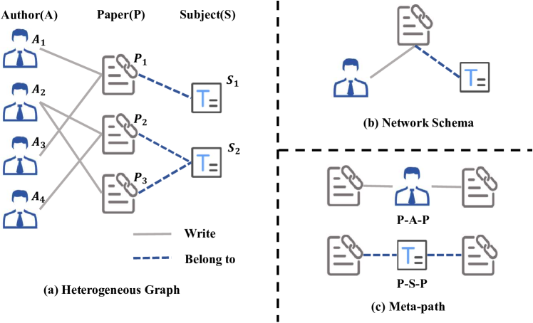
Network Schema: The network schema, denoted as $T_{G}=(I,J)$, is used to demonstrate the high-level topology of an HIN, which describes the node types and their interaction relations. The network schema itself is a directed graph that is predicated on a collection of node types $I$, where the links between them are represented by the set of relational edge types $J$. The network schema for the ACM is depicted in the top portion of Figure 2 (b).

Meta-path: In an $\operatorname{HIN}G=(V,E,I,J,\phi,\varphi)$, a meta-path $\rho$ is represented as $I_{1}\stackrel{{\scriptstyle J_{1}}}{{\longrightarrow}}I_{2}\stackrel{{\scriptstyle J_{2}}}{{\longrightarrow}}\ldots\stackrel{{\scriptstyle J_{l}}}{{\longrightarrow}}I_{l+1}$, describing a composite connection between $v_{1}$ and $v_{l}$. Taking Figure 2 as an instance, multiple meta-paths, like “Paper-Author-Paper (PAP)” and “Paper-Subject-Paper (PSP)” can link entities within the HIN. Commonly, different meta-paths can reveal the different inter-dependency information of two movies. The path “PAP” indicates that two papers were written by the same author, while “PSP” illustrates that two papers are of the same subject.

Figure 3. The training framework of our proposed GC-HGNN. (a) The model respectively takes the entire heterogeneous graph and the views based on meta-paths, dividing them into inputs for the network schema View and the meta-path view; (b) the network schema view employs an attention mechanism to focus on one-hop neighbors of each node; (c) the meta-path view utilizes a masked autoencoder to generate views for intra-contrast; (d) the hierarchical contrast uses a proposed dynamic sampling mechanism to generate more hard negative samples to enhance the discriminator.

4. THE PROPOSED MODEL

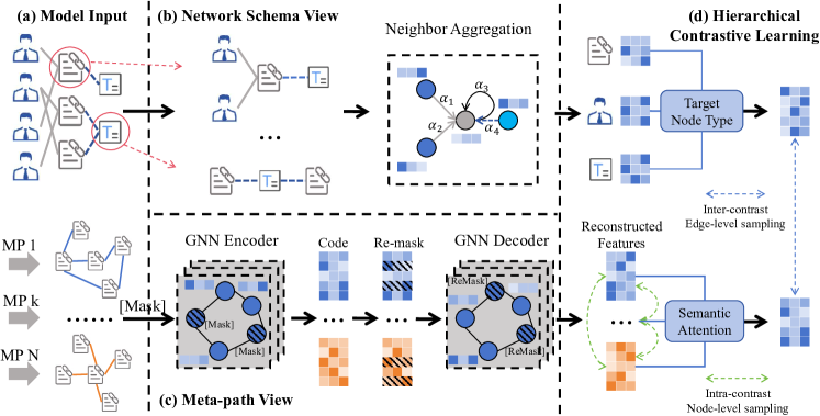
In this section, our overall framework and brief module descriptions are shown in Figure 3. We then provide detailed explanations for each module following the framework’s order. Finally, we propose different optimization strategies based on the downstream tasks.

4.1. Network Schema View

This section typically takes the entire heterogeneous information network as input, as shown in Figure 3 (a). First, we consider each node in the network as an anchor, forming a subnetwork that includes all the one-hop neighbor nodes. For example, in Figure 3 (b), the subgraph indicated by the circles represents the subnetwork composed of the target node. Next, we put such subnetworks into a heterogeneous neighbor aggregation network, utilizing attention mechanisms to obtain node embeddings. Finally, we select the all embeddings of the desired target node for downstream tasks. Specific implementation process: We project all nodes into the same node space ($\boldsymbol{P}_{r}$ is projection matrix) because the subnetworks contain different node types. We define $e$ as the current node computing the attention score and $\boldsymbol{h}_{e}^{0}$ as its initial embedding. Next, we learn specific aggregation functions for different types of edges to compute attention scores:

(1) $$\alpha_{ew}=\frac{\exp\left(f_{r}\left(\boldsymbol{h}_{e}^{0},\boldsymbol{P}_{r}\boldsymbol{h}_{w}^{0}\right)\right)}{\sum_{j\in\mathcal{N}_{1}(e)}\exp\left(f_{r}\left(\boldsymbol{h}_{e}^{0},\boldsymbol{P}_{r}\boldsymbol{h}_{j}^{0}\right)\right)},\quad\forall w\in\mathcal{N}_{1}(e)\\$$

where $f_{r}(\cdot,\cdot)$ denotes the deep neural network designed to execute attention mechanisms over one-hop neighbors. Here, $\alpha_{ew}$ represents the influence level for neighbor node $w$, and $\mathcal{N}_{1}(e)$ denotes the set of one-hop neighbor nodes of $e$. Finally, we aggregate the following information from $\mathcal{N}_{1}(e)$:

(2) $$\boldsymbol{h}_{e}^{1}=\sigma\left(\sum_{w\in\mathcal{N}_{1}(e)}\alpha_{ew}\boldsymbol{h}_{w}^{0}\right)$$

where $\sigma$ denotes the activation function.

4.2. Meta-path View

In this part, model input are multi-views constructed from different meta-paths. For example, in Figure 3 (a), we connect two nodes of the same type using the specified meta-path ‘PAP’. Thus, such a graph composed of nodes of the same type is referred to as a view based on the meta-path ‘PAP’. Based on preliminaries, we define a set of meta-paths as $\left\{\rho_{1},\ldots,\rho_{j},\ldots,\rho_{M}\right\}$, and the corresponding views are $\left\{G^{\rho_{1}},G^{\rho_{2}},\ldots,G^{\rho_{M}}\right\}$. $M$ is the number of meta-paths we have selected. Here, the model defines a graph $\mathcal{G}=(\mathcal{V},\boldsymbol{A},\boldsymbol{X})$. For each graph, $\mathcal{V}$ is the node set, $N=$ $|\mathcal{V}|$ is the number of nodes, $\mathbf{A}\in\{0,1\}^{N\times N}$ is the adjacency matrix, and $\mathbf{X}\in\mathbb{R}^{N\times d}$ is the input node feature matrix.

First, we employ a non-replacement random sampling strategy to select a set of nodes $\mathcal{V}^{[Mask]}$ from the entire set of nodes $\mathcal{V}$.

(3) $$\mathcal{V}^{[Mask]}=\{\mathcal{V}_{i}\in\mathcal{V}\mid r_{i}\leq p\},r_{i}\sim\text{Uniform}(0,1)$$

where $p$ is the mask ratio we set. Uniform random sampling helps the encoder avoid potential bias centers, which refers to the bias arising when all neighbors of a node are either completely masked or completely visible. We mask the entire node features in the set $\mathcal{V}^{[Mask]}$ to obtain $\widetilde{\boldsymbol{X}}$.

Then, we input the masked features into a GNN encoder to obtain the output. To better reconstruct the features, we set the encoder with adjustable layers $L$. A multi-layer encoder typically captures distant neighbors to expand their receptive field, enriching their representations.

(4) $$\boldsymbol{H}=f_{E}^{(L)}(\boldsymbol{A},\widetilde{\boldsymbol{X}})$$

where $\widetilde{\boldsymbol{X}}$ is feature input with the $[Mask]$, and $\boldsymbol{H}\in\mathbb{R}^{N\times d}$ denotes code after the encoder. Next, to further encourage the decoder to learn compressed representations, we use a new ratio and the same sampling strategy to mask a different set of nodes $\mathcal{V}^{[ReMask]}$. We use a GNN with the same structure as the encoder to act as the decoder. However, the decoder can be GAT (Velickovic et al., 2017), GCN (He et al., 2020a), and its layer number and type can be independent of the encoder’s.

(5) $$\boldsymbol{H}_{Re}=f_{D}^{(L)}(\boldsymbol{A},\widetilde{\boldsymbol{H}})$$

where $\widetilde{\boldsymbol{H}}$ is decoder input with the $[Remask]$, and $\boldsymbol{H}_{Re}$ as the reconstructed output under meta-path view. We perform multiple masking operations between encoders, equivalent to the masked nodes reconstructing their features through their neighbors. The uniform sampling strategy ensures that each reconstructed node receives the same supervised signals. Such an autoencoder helps train robust node embeddings and mitigates the impact of noise from the meta-path view.

Finally, based on the mentioned meta-path-based multi-view, we denote the reconstructed features obtained from the different views as $\left\{\boldsymbol{H}_{Re}^{\rho_{1}},\ldots,\boldsymbol{H}_{Re}^{\rho_{j}},\ldots,\boldsymbol{H}_{Re}^{\rho_{M}}\right\}$. We employ a semantic attention mechanism to assign weights to each view to balance their importance in downstream tasks.

(6) $$w_{\rho_{j}}=\frac{1}{|\mathcal{V}|}\sum_{\boldsymbol{e}\in\mathcal{V}}\boldsymbol{q}^{T}\cdot\tanh\left(\boldsymbol{W}{\boldsymbol{h}_{Re}^{\rho_{j}}}+b\right)$$

where ${\boldsymbol{h}_{Re}^{\rho_{j}}}$ is a reconstructed feature of a node under meta-path $\rho_{j}$. $\boldsymbol{q}^{T}$ and $\boldsymbol{W}$ are query vectors and weight matrices to ensure that the dimensions and feature spaces match different views, respectively. Next, the weight for $\rho_{j},(j=1:N)$ is defined as:

(7) $$\gamma_{\rho_{j}}=\frac{\exp\left(w_{\rho_{j}}\right)}{\sum_{j=1}^{N}\exp\left(w_{\rho_{j}}\right)}$$

where $\gamma_{\rho_{j}}$ denotes the weight of meta-path $\rho_{j}$. According to the attention mechanism, when the semantic attention score $\gamma_{\rho_{j}}$ is higher, it indicates the meta-path $\rho_{j}$ gets more importance in downstream tasks. We aggregate feature embeddings from all meta-paths to obtain the final node features under the meta-path view.

(8) $$\boldsymbol{h}_{e}^{2}=\sum_{j=1}^{N}\gamma_{\rho_{j}}\cdot\boldsymbol{h}_{e}^{\rho_{j}}$$

4.3. Hierarchical Contrastive learning

The model employs two sampling strategies. For intra-contrast, it uses a node-level contrast, whereas for inter-contrast, it adopts an edge-level contrast. Edge-level sampling is illustrated in Figure 4. Next, we get an edge sampling set $\mathcal{E}$.

Figure 4. Our GC-HGNN proposed a hard sampling strategy for inter-contrast. Location-aware Pos: the green node uses metapath2vec (Dong et al., 2017) to perceive the location within a heterogeneous graph to obtain node embeddings. Semantic-aware Pos: The blue node is connected to the anchor node through all types of meta-paths, indicating the semantic similarity between them.

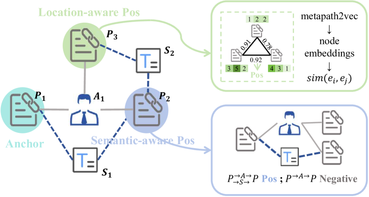
Intra-contrast. First, we utilize sampling set $\mathcal{E}$ to select the positive sample set $\widetilde{\mathcal{V}}$ for node-level contrast based on the degree of nodes. High-degree nodes have more connections in the graph and are more likely to capture the central structure and important patterns in the graph. The embeddings of the model, based on multi-views, are denoted by $\left\{\boldsymbol{H}_{Re}^{\rho_{1}},\ldots,\boldsymbol{H}_{Re}^{\rho_{j}},\ldots,\boldsymbol{H}_{Re}^{\rho_{M}}\right\}$. Next, we take these embeddings as input to obtain a multi-view loss. Intra-contrast employs scaled cosine error (SCE) (Grill et al., 2020) as the contrastive loss between multi-views. SCE has been proven to focus on hard samples in the data to improve the stability of representation learning.

(9) $$\mathcal{L}_{Intra}=\frac{1}{|\widetilde{\mathcal{V}}|}\sum_{v_{i}\in\widetilde{\mathcal{V}}}\left(1-\frac{\boldsymbol{x}_{i}^{T}\boldsymbol{z}_{i}}{\left\|\boldsymbol{x}_{i}\right\|\cdot\left\|\boldsymbol{z}_{i}\right\|}\right)^{\eta},\eta\geq 1$$

where $\boldsymbol{x}$ and $\boldsymbol{z}$ respectively denote embeddings of the same node under two meta-path views. During training, we can scale the cosine error by a power of $\eta\geq 1$ to minimize the differences of important samples under multi-views.

Inter-contrast. Inter-contrast performs collaborative contrastive learning between two non-aligned views. In set $\mathcal{E}$, we define the target node to be sampled as $i$ and the connected nodes to it as a positive set $\mathbb{P}_{i}$, inspired by (Wang et al., 2021). Otherwise, they form the negative sample set $\mathbb{N}_{i}$. From the perspective of the scale of $\mathcal{E}$ and $\widetilde{\mathcal{V}}$, inter-contrast typically has more hard negative samples, and thus, its supervisory role is more evident. The contrastive loss of the network schema view with respect to the meta-path view is as follows:

(10) $$\mathcal{L}_{Inter}^{1}=-\log\frac{\sum_{j\in\mathbb{P}_{i}}\exp\left(\operatorname{sim}\left(h_{i}^{1},h_{j}^{2}\right)/\tau\right)}{\sum_{k\in\left\{\mathbb{P}_{i}\cup\mathbb{N}_{i}\right\}}\exp\left(\operatorname{sim}\left(h_{i}^{1},h_{k}^{2}\right)/\tau\right)}$$

where $\operatorname{sim}(i,j)$ is the cosine similarity, and $\tau$ denotes a temperature parameter. Inter-contrast utilizes mutual contrast between the two views to achieve the collaborative process. The contrastive loss of the meta-path view with respect to the network schema view is $\mathcal{L}_{Inter}^{2}$. The overall inter-contrast losses are as follows:

(11) $$\mathcal{L}_{{Inter}}=\frac{1}{|\mathcal{E}|}\sum_{i\in\mathcal{E}}\left[\lambda\cdot\mathcal{L}_{Inter}^{1}+(1-\lambda)\cdot\mathcal{L}_{Inter}^{2}\right]$$

where $\lambda$ is a balance coefficient to control the weight of each view pair. We employed intra-contrast and inter-contrast for hierarchical contrastive learning and conducted analyses on their operational mechanisms. The intra-contrast assumes that meta-paths are interconnected and aim to maximize their mutual information. This method integrates the different semantics across meta-paths to form a generalized knowledge representation for downstream tasks. On the other hand, the inter-contrast approach attempts to enhance node representation by contrasting local and global information, preventing nodes from being influenced by noise from higher-order neighbors. The hierarchical contrast and sampling strategies are designed to construct a useful discriminator to enhance the adversarial interplay between the generative and contrastive models.

4.4. Model Optimization

In this subsection, we describe the optimization strategies for different tasks in our experiments. It has two aspects: node classification and link prediction.

Node classification. First, for the node classification task (Wang et al., 2019, 2021, 2023), the common practice is to train embeddings for all nodes using self-supervised loss. Then, we fine-tune the model on different datasets using a few labeled samples and a single-layer MLP. The node-level and edge-level strategies we propose typically lead to considerable loss differences in the initial phase. Therefore, it is necessary to balance their weights during the training phase. The loss generated by hierarchical contrastive learning is as follows:

(12) $$\mathcal{L}_{hcl}=\lambda_{Intra}\cdot\mathcal{L}_{{Intra}}+\lambda_{Inter}\cdot\mathcal{L}_{{Inter}}$$

where $\lambda_{{Intra}}$ and $\lambda_{{Inter}}$ are hyper-parameters to balance the influences of $\mathcal{L}_{{Intra}}$ and $\mathcal{L}_{{Inter}}$, respectively.

Link prediction. Next, for the link prediction task (Chen et al., 2023; Shi et al., 2018), we introduce the Bayesian Personalized Ranking Loss (BPR) (Rendle et al., 2012). This loss function treats two connected nodes as a positive pair and two unconnected nodes as a negative pair. Its objective is to maximize the scores between positive pairs and negative pairs. Formally, the BPR loss is defined as follows:

(13) $$\mathcal{L}_{bpr}=-\frac{1}{|\mathcal{O}|}\sum_{(i,j,k)\in O}\log\sigma\left(d_{i}^{\top}d_{j}-d_{i}^{\top}d_{k}\right)$$

where $\mathcal{O}=\left\{(i,j,k)\mid A_{i,j}=1,A_{i,k}=0\right\}$ is the training data. We combine $\mathcal{L}_{{hcl}}$ and $\mathcal{L}_{bpr}$ to get the link prediction loss.

(14) $$\mathcal{L}=\lambda_{hcl}\cdot\mathcal{L}_{{hcl}}+\lambda_{bpr}\cdot\mathcal{L}_{{bpr}}$$

where $\lambda_{hcl}$ and $\lambda_{bpr}$ denote hyperparameters used to balance task weights.

Time complexity analysis. The network schema view’s time complexity is $O\left(|V|\cdot D_{n}d^{2}\right)$, where $|V|$ denotes the edge number of a heterogeneous graph. $D_{n}$ is the average node degree and $d$ is the feature dimension. For the meta-path view, GC-HGNN has $M$ meta-path-based subgraphs. So, the time complexity of the meta-path view is $O\left(|\mathcal{V}|\cdot 2MLDd\right)$, where $L$ is the number of GNN layers. Then, the self-supervised loss contains $\lambda_{Intra}$ and $\lambda_{Inter}$. The time complexity to get positive samples and calculate $\lambda_{Intra}$ is $O\left(|\widetilde{\mathcal{V}}|\cdot d\right)$. For the $\lambda_{Inter}$, the complexity is $O\left(|\mathcal{V}|^{2}\cdot d\right)$. Because the edge set $\mathcal{E}$ is a matrix $\mathcal{E}\in\{0,1\}^{N\times N}$ composed of target nodes. In the link prediction task, the complexity of the additional $\mathcal{L}_{{bpr}}$ is $O\left(|\mathcal{O}|\cdot d\right)$. Thus, the overall time complexity of GC-HGNN is $O\left(|V|\cdot D_{n}d^{2}+|\mathcal{V}|\cdot 2MLD_{m}d+|\widetilde{\mathcal{V}}|\cdot d+|\mathcal{V}|^{2}\cdot d+|\mathcal{O}|\cdot d\right)$. This complexity is the time complexity for each epoch during training, and the overall training time will be determined by the number of training epochs.

5. EXPERIMENT

In this section, we conduct extensive experiments and answer the following research questions:

• RQ1: How does GC-HGNN perform w.r.t. node classification task?

• RQ2: How does GC-HGNN perform w.r.t. link prediction task?

• RQ3: Are the key components in our GC-HGNN delivering the expected performance gains?

• RQ4: How does GC-HGNN combine contrast and generation to achieve performance beyond one or the other?

• RQ5: How do different settings influence the effectiveness of GC-HGNN?

Table 1. Statistics of datasets used in this paper.

lccccc Dataset Nodes Edges Relations Task
ACM 11,246 34,852 2 Node Classification
DBLP 26,128 239,566 3 Node Classification
Aminer 55,783 153,676 2 Node Classification
Freebase 43,854 151,043 3 Node Classification
Last.fm 31,469 913,216 4 Link Prediction
Yelp 31,092 976,276 5 Link Prediction
Douban Movie 37,595 3,429,882 6 Link Prediction
Douban Book 51,029 4,451,894 7 Link Prediction

Table 2. Quantitative results (%) on node classification.

c—c—cccccccc Methods Data ACM DBLP Aminer Freebase
Macro-F1 Micro-F1 Macro-F1 Micro-F1 Macro-F1 Micro-F1 Macro-F1 Micro-F1
DeepWalk(2017) $\mathbf{A}$ $68.34\pm 0.42$ $74.05\pm 0.47$ $89.24\pm 0.49$ $90.12\pm 0.45$ $68.48\pm 0.38$ $74.00\pm 0.41$ $59.20\pm 0.50$ $59.85\pm 0.43$
MP2vec(2017) $\mathbf{A}$ $68.05\pm 0.98$ $72.86\pm 0.92$ $89.98\pm 0.84$ $90.30\pm 0.38$ $66.28\pm 1.17$ $72.21\pm 0.84$ $55.50\pm 0.49$ $53.17\pm 0.34$
HERec(2018) $\mathbf{A}$ $68.84\pm 0.44$ $74.45\pm 0.45$ $89.44\pm 0.67$ $90.37\pm 0.47$ $68.73\pm 0.83$ $74.21\pm 0.87$ $59.46\pm 1.16$ $60.11\pm 0.46$
HAN(2019) $\mathbf{X},\mathbf{A},\mathbf{Y}$ $88.30\pm 0.23$ $88.20\pm 0.37$ $86.00\pm 0.53$ $85.18\pm 0.49$ $64.15\pm 0.35$ $75.60\pm 0.79$ $58.50\pm 0.93$ $61.30\pm 0.41$
HGT(2020) $\mathbf{X},\mathbf{A},\mathbf{Y}$ $87.09\pm 0.35$ $88.20\pm 0.26$ $91.36\pm 0.23$ $91.24\pm 0.49$ $64.15\pm 0.35$ $75.60\pm 0.24$ $58.30\pm 0.72$ $61.34\pm 0.18$
MHGCN(2022) $\mathbf{X},\mathbf{A},\mathbf{Y}$ $88.86\pm 0.63$ $88.70\pm 0.22$ $90.62\pm 0.58$ $90.62\pm 0.19$ $71.34\pm 0.10$ $79.24\pm 0.79$ $57.12\pm 0.32$ $59.30\pm 0.33$
DMGI(2020) $\mathbf{X},\mathbf{A}$ $87.66\pm 0.24$ $87.60\pm 0.35$ $89.55\pm 0.52$ $90.66\pm 0.46$ $63.15\pm 0.21$ $66.61\pm 0.38$ $55.99\pm 0.59$ $59.37\pm 0.27$
HeCo(2021) $\mathbf{X},\mathbf{A}$ $88.56\pm 0.28$ $88.71\pm 0.43$ $90.26\pm 0.37$ $90.59\pm 0.25$ $71.64\pm 0.22$ $79.95\pm 0.55$ $59.87\pm 0.33$ $62.33\pm 0.40$
HGCML(2023) $\mathbf{X},\mathbf{A}$ $88.46\pm 0.38$ $87.90\pm 0.27$ $90.47\pm 0.33$ $91.11\pm 0.49$ $71.84\pm 0.45$ $78.30\pm 0.49$ $58.92\pm 2.57$ $62.71\pm 0.23$
HGMAE(2023) $\mathbf{X},\mathbf{A}$ $89.29\pm 0.36$ $89.15\pm 0.31$ $91.60\pm 0.58$ $91.89\pm 0.35$ $72.63\pm 0.27$ $79.87\pm 0.42$ $60.82\pm 0.51$ $63.89\pm 0.38$
GC-HGNN $\mathbf{X},\mathbf{A}$ $\mathbf{90.54}\pm\mathbf{0.28}$ $\mathbf{90.36}\pm\mathbf{0.31}$ $\mathbf{92.54}\pm\mathbf{0.36}$ $\mathbf{93.01}\pm\mathbf{0.30}$ $\mathbf{73.44}\pm\mathbf{0.20}$ $\mathbf{81.28}\pm\mathbf{0.32}$ $\mathbf{62.47}\pm\mathbf{0.42}$ $\mathbf{65.85}\pm\mathbf{0.35}$

5.1. Experimental Setings

5.1.1. Datasets

The performance of GC-HGNN has been validated on six real-world datasets. These datasets encompasses four datasets for node classification: ACM, DBLP, Aminer, and Freebase, as well as four datasets for link prediction: Last.fm, Yelp, Douban Movie and Douban Book. A statistical overview of all the datasets is presented in Table 5.

Datasets for Node Classification.

• ACM (Han et al., 2022). The target nodes are papers, which are divided into three classes. For each paper, there are 3.33 authors averagely, and one subject.

• DBLP (Fu et al., 2020). The target nodes are authors, which are divided into four classes. For each author, there are 4.84 papers averagely.

• Freebase (Tian et al., 2023). The target nodes are movies, which are divided into three classes. For each movie, there are 18.7 actors, 1.07 directors and 1.83 writers averagely.

• Aminer (Wang et al., 2021). The target nodes are papers. We extract a subset of original dataset, where papers are divided into four classes. For each paper, there are 2.74 authors and 8.96 references averagely.

Datasets for Link Prediction.

• Last.fm. The music recommendation dataset contains three types of nodes: user, artist, and tag, along with four edge relationships. We predict whether there is an interaction between a user and an artist.

• Yelp. The business recommendation dataset contains five types of nodes, including user, business, and city, along with five edge relationships. We predict whether there is an interaction between a user and an business.

• Douban Movie. The movie recommendation dataset contains six types of nodes, including user, movie, and actor, as well as six edge relationships. We predict the interactions between a user and a movie.

• Douban Book (Shi et al., 2018). The book recommendation dataset contains seven types of nodes, including user, book, and author, as well as seven edge relationships. We predict the interactions between a user and a book.

5.1.2. Baselines

We respectively select the most representative baseline model for node classification and link prediction.

Heterogeneous Graph Representation Learning Models.

• DeepWalk (Perozzi et al., 2014) maps network structure to vector space via random walks, preserving neighbor similarity.

• MP2vec (Dong et al., 2017) employs meta-path-guided random walks for heterogeneous network embeddings.

• HERec (Shi et al., 2018) integrates meta-path-based random walks for node embeddings in HINs with fusion functions.

• HAN (Wang et al., 2019) employs node-level and semantic-level attention to capture node and meta-path importance.

• HGT (Hu et al., 2020a) introduces a novel architecture for handling heterogeneous structures in Web-scale graphs.

• DMGI (Park et al., 2020) achieves self-supervised learning by meta-path-based networks and mutual infromation between networks.

• HeCo (Wang et al., 2021) uses collaborative supervised contrast between network schema view and meta-path view.

• MHGCN (Yu et al., 2022a) utilizes multi-layer convolution aggregation to capture meta-path interactions of different lengths.

• HGCML (Wang et al., 2023) uses meta-paths to generate multi-views combined with comparative learning between views.

• HGMAE (Tian et al., 2023) captures comprehensive graph information by reconstructing masked meta-path-based view and embedding.

Graph Recommendation Models.

• BPRMF (Rendle et al., 2012) learns implicit feature vectors between users and items to maximize difference in pairwise preferences.

• LightGCN (He et al., 2020a) removes the feature transformation and nonlinear activations of GCN to achieve light recommendation.

• SGL (Wu et al., 2021) generates contrast views by edge dropout to aid contrastive learning to enhance recommendation.

• SMIN (Long et al., 2021) utilizes metagraph informax network to enhance user preference representation for social recommendation.

• NCL (Lin et al., 2022) considers the relationship between neighbor nodes to enhance collaborative filtering.

• HGCL (Chen et al., 2023) integrates heterogeneous relational semantics by leveraging contrastive self-supervised learning.

• VGCL (Yang et al., 2023) introduces a variational graph reconstruction for graph augmentation to achieve light and robust recommendation.

5.2. Node Classification (RQ1)

The experiment results are shown in Table 5. Our experiments follow the settings of OpenHGNN (Han et al., 2022), a comprehensive and unified open-source platform. We categorize the baseline methods into three classes based on the input: unsupervised, supervised, and self-supervised. The symbols $\mathbf{X}$, $\mathbf{A}$, and $\mathbf{Y}$ in the table refer to the node features, graph structure, and predicted node labels, respectively.

Our GC-HGNN demonstrates state-of-the-art model (SOTA) performance on all datasets. Notably, self-supervised methods generally outperform shallow unsupervised methods. This is because unsupervised models only consider the graph structure, while self-supervised models attempt to mine hidden semantic relationships from the HIN. On the other hand, the performance of supervised models relies on more labels, which goes against the challenge of label scarcity and preciousness. HGMAE, as a generative reconstruction model, showcases the enormous potential of autoencoders in graph representation learning, and HeCo, as a contrastive model, also achieves remarkable results. These two models learn graph representations from different perspectives, providing ideas for designing subsequent graph neural network models. Inspired by this, GC-HGNN combines the generative masked autoencoder with a contrastive discriminator to enhance performance in contrastive learning by generating more hard negative samples.

5.3. Link Prediction (RQ2)

The recommendation has become a classic task for heterogeneous link prediction due to its wide application range. Considering the task adaptability, we apply LightGCN (He et al., 2020a) for the network schema. Here, we unify the embedding dimension to 64 and select the classic recall and NDCG (Zhang et al., 2023) as evaluation metrics. It is worth mentioning that our GC-HGNN compares with the latest general recommendation models.

The results are shown in Table 5.3. The first part presents the MF models, followed by general recommendation models, and the last part showcases specialized HGNN models. It can be observed that NCL and HGCL, as representatives of contrastive learning, demonstrate clear advantages over other models in their respective categories. The essence of contrastive learning lies in uniformity and alignment. However, modifying the graph structure to achieve uniformity is time-consuming and tricky, so it is better to consider this aspect from the perspective of the embedding space. Our GC-HGNN incorporates embeddings learned from the meta-path view into the network schema view and performs hierarchical contrastive learning. Such embeddings can better help the model learn a more uniform distribution because each meta-path brings different semantic information. Finally, across multiple datasets, our model achieved improvements of over 3% compared to the strongest baseline models, demonstrating the effectiveness of our model in aligning different meta-paths and perspectives.

Table 3. Quantitative results on link prediction.

c—cccccccc Dataset Douban-Book Douban-Movie Last.fm Yelp
Metric Recall@20 NDCG@20 Recall@20 NDCG@20 Recall@20 NDCG@20 Recall@20 NDCG@20
BPRMF(2012) 0.1302 0.1112 0.1678 0.1888 0.2400 0.2349 0.0752 0.0466
HERec(2018) 0.1313 0.1201 0.1714 0.1919 0.2526 0.2484 0.0822 0.0471
LightGCN (2020) 0.1412 0.1307 0.1791 0.2011 0.2623 0.2638 0.0893 0.0565
SGL-ED (2021) 0.1685 0.1631 0.1890 0.2056 0.2724 0.2704 0.0971 0.0614
NCL (2022) 0.1694 0.1623 0.1910 0.2074 0.2738 0.2718 0.0975 0.0623
VGCL (2023) 0.1701 0.1602 0.1933 0.2097 0.2740 0.2726 0.0978 0.0621
HAN (2019) 0.1290 0.1137 0.1676 0.1884 0.2443 0.2397 0.0767 0.0449
HGT (2020) 0.1308 0.1157 0.1696 0.1904 0.2463 0.2417 0.0787 0.0469
SMIN (2021) 0.1353 0.1239 0.1718 0.1909 0.2547 0.2560 0.0847 0.0485
HGCL (2023) 0.1526 0.1426 0.1868 0.2024 0.2684 0.2688 0.0954 0.0607
GC-HGNN $\mathbf{0.1890}$ $\mathbf{0.1717}$ $\mathbf{0.1997}$ $\mathbf{0.2175}$ $\mathbf{0.2813}$ $\mathbf{0.2795}$ $\mathbf{0.1044}$ $\mathbf{0.0649}$
Improv. $11.11\%$ $7.18\%$ $3.31\%$ $3.72\%$ $2.63\%$ $2.53\%$ $6.75\%$ $4.51\%$

(a) ACM

(b) DBLP

(c) Aminer

(d) Freebase

Figure 5. The comparison of GC-HGNN and its variants.

5.4. Ablation Study(RQ3)

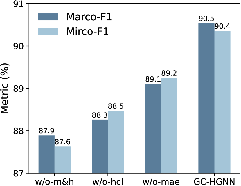
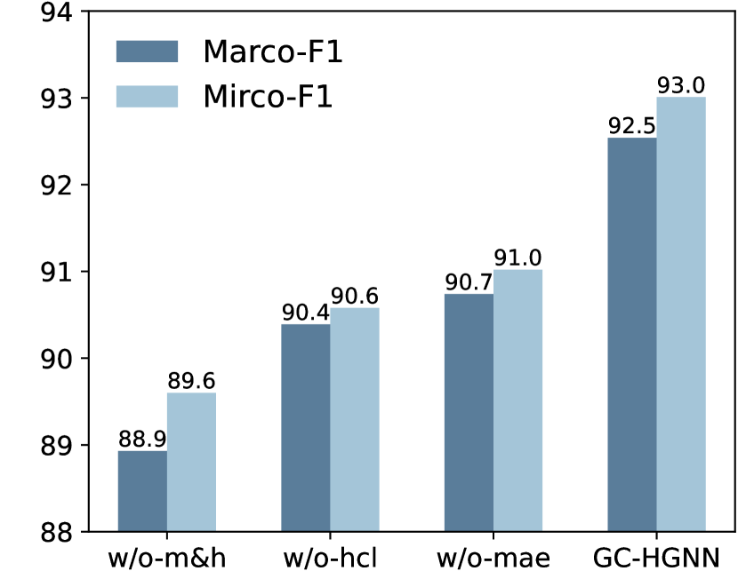
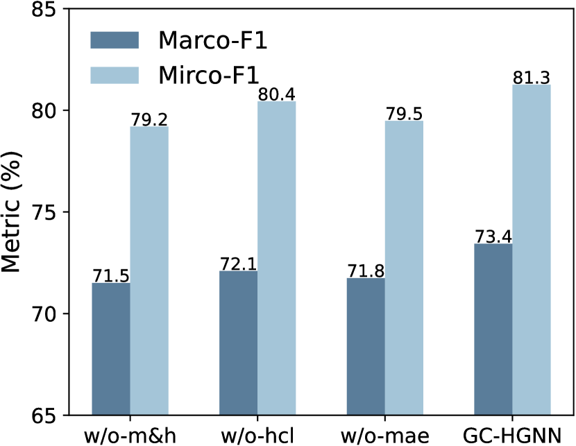
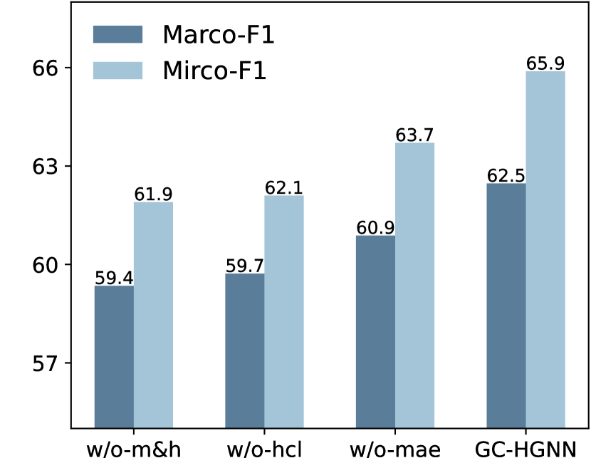
In this subsection, we conducted ablation experiments to validate the effectiveness of key components in our GC-HGNN and made possible explanations regarding the experimental results. Here are three variants for our model.

• $\boldsymbol{w}/\boldsymbol{o}{-}\mathbf{mae}$: This variant replaces the masked autoencoder (MAE) of the meta-path view with a normal GAT (Velickovic et al., 2017) encoder.

• $\boldsymbol{w}/\boldsymbol{o}{-}\mathbf{hcl}$: This variant cancels the hierarchical contrastive learning (HCL) module and directly uses the InfoNCE loss for downstream tasks.

• $\boldsymbol{w}/\boldsymbol{o}{-}\mathbf{m\&h}$: The third variant simultaneously removes the masked autoencoder (MAE) and hierarchical contrastive learning (HCL) modules.

As shown in Figure 5, it can be observed that, in all cases, removing the HCL module results in worse performance compared to other variants. Additionally, variants where mae and HCL are removed generally exhibit the worst performance in most cases. This further highlights two important points: 1) The graph structural information is overemphasized, and reconstructing the graph links is not necessary; 2) The existing heterogeneous contrastive learning strategies are not sufficient to serve as good discriminators to enhance the masked autoencoder effectively.

(a) MP2vec

(b) HeCo

(c) HGMAE

(d) GC-HGNN

Figure 6. Embedding visualization of DBLP dataset. Different colors indicate different node category labels.

(a) ACM

(b) DBLP

(c) Aminer

(d) Freebase

Figure 7. The impact wrt. hierarchical contrast coefficient.

(a) Macro-F1 wrt. dimension

(b) Micro-F1 wrt. dimension

(c) Macro-F1 wrt. mask ratio

(d) Micro-F1 wrt. mask ratio

Figure 8. The impact wrt. dimension and mask ratio. The axes on the left belong to the ACM and DBLP datasets and the axes on the right belong to other datasets.

5.5. Interpretability and Visualization (RQ4)

In this study, we focus on discussing the various modules of GC-HGNN, attempting to provide a rational concept or explanation. We investigated the advantages of generative-contrastive model, and then further illustrate the motivation through the representation visualization.

Interpretability. Generative-contrastive representation learning (Wu et al., 2023; Yang et al., 2023; Goodfellow et al., 2020) utilizes discriminative loss functions as objectives, aiming to address some inherent shortcomings of generative reconstruction, such as sensitive and conservative distribution and low-level abstraction objective. In contrastive learning (Chen et al., 2020; Wang et al., 2021; He et al., 2020b; Wu et al., 2021), we can alleviate these issues by setting up appropriate discriminators to learn ‘distinguishable’ information for different samples. However, the encoder and decoder brought by generative learning (Devlin et al., 2018; Hou et al., 2022; Tian et al., 2023; Chowdhery et al., 2023) endow it with powerful embedding expression capabilities. The decoder requires the representation to be reconstructable, meaning that it contains all the information of the input. Furthermore, generative-contrastive self-supervised methods abandon the point-to-point reconstruction objective and instead pursue the alignment of distributions in the data. In summary, adversarial methods (Liu et al., 2021) absorb the advantages of both generative and contrastive methods, but also face the challenge of how to build a framework in the field of heterogeneous graphs. We propose a masked autoencoder to enhance the expressive power of meta-path perspectives, and then use hierarchical contrastive learning and designed sampling strategies to serve as enhanced discriminators. Experiments demonstrate that this is an effective and novel exploration.

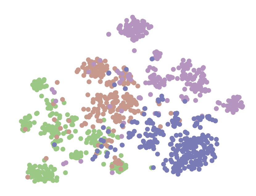
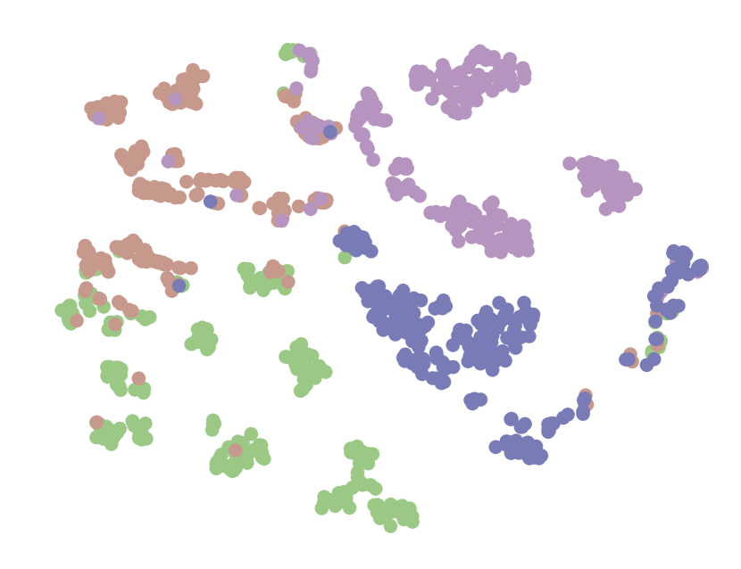
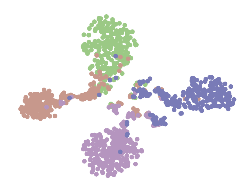
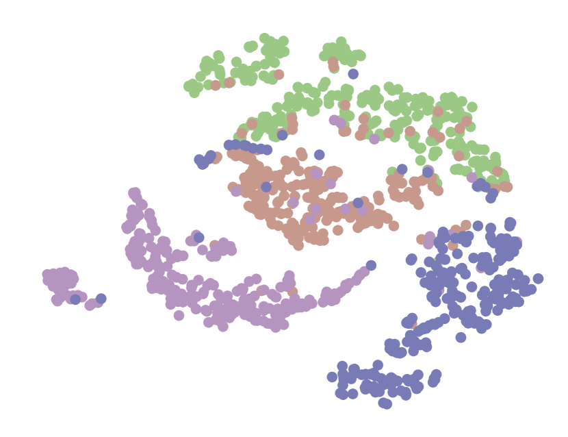
Visualization. To more intuitively perceive the embeddings of different models, we use t-SNE (Van der Maaten and Hinton, 2008) to reduce the dimensionality of the embeddings and visualize them with labels. As shown in Figure 6, we select three representative models: unsupervised MP2vec, contrastive HeCo, and generative HGMAE. We can observe that MP2vec performs the worst, with different types of nodes mixed together and difficult to distinguish. HeCo can effectively differentiate categories, but each block is separated and does not form obvious clusters. HGMAE uses a hidden dimension of 256 and is a generative method, thus exhibiting more evident clustering phenomena. However, our GC-HGNN is based on a contrastive framework and demonstrates both clustering and uniform distribution, balancing the advantages of contrastive and generative approaches. This phenomenon also indicates that our generative-contrastive paradigm is effective.

5.6. Parameter Sensitivity (RQ5)

In this study, we explored the impact of key hyperparameters on heterogeneous graph node classification. We investigated the effects of hierarchical contrast coefficient, embedding dimension and positive samples.

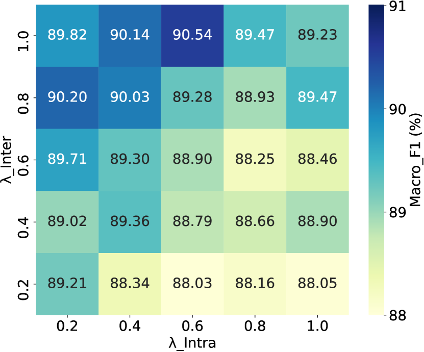
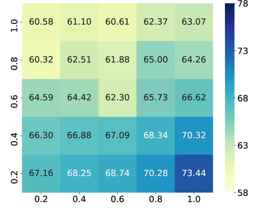
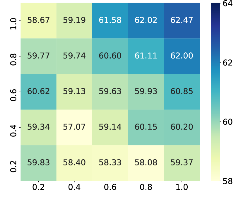
Hierarchical contrast coefficient. As shown in Section 4.4, the $\mathcal{L}_{hcl}$ contains $\lambda_{{Intra}}$ and $\lambda_{{Inter}}$, which are set from 0 to 1 with an increment. In Figure 7, we can observe that except for the Aminer dataset, the performance of other datasets improves as $\lambda_{{Inter}}$ increases. This phenomenon follows the principle of our proposed sampling method, where inter-contrast has more hard negative samples compared to intra-contrast.

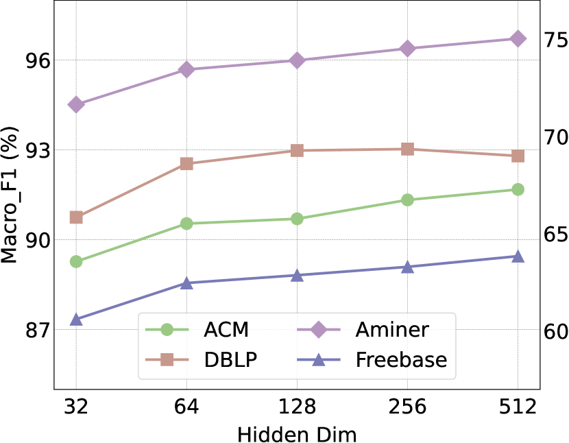
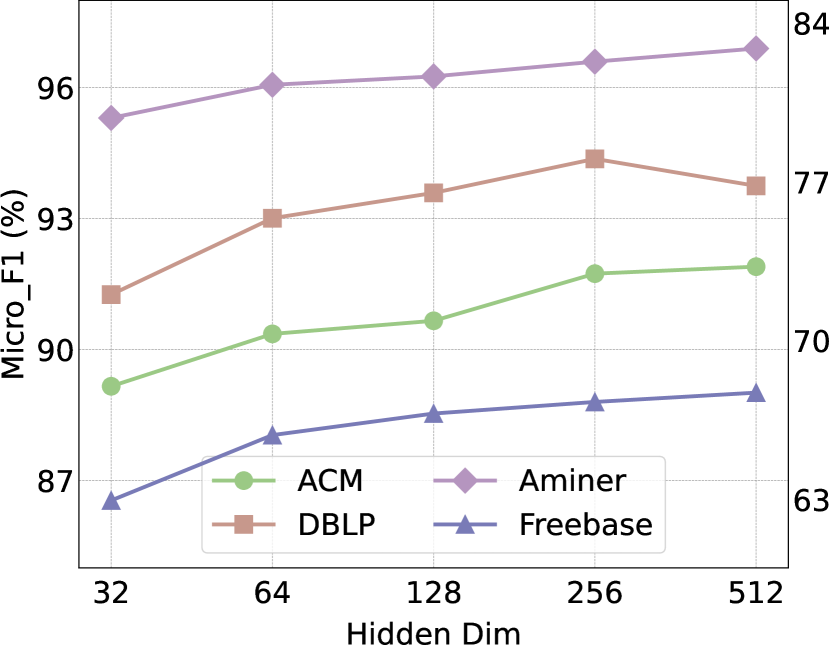
Embedding dimension. We investigated how different embedding sizes affect node classification performance from 32 to 512. Figure 8 shows that most datasets improved up to a 512-dimensional embedding, apart from DBLP, which peaked at 256. However, to balance the marginal gains against higher computational costs and overfitting risks, we standardized the embedding size to 64 for all tests.

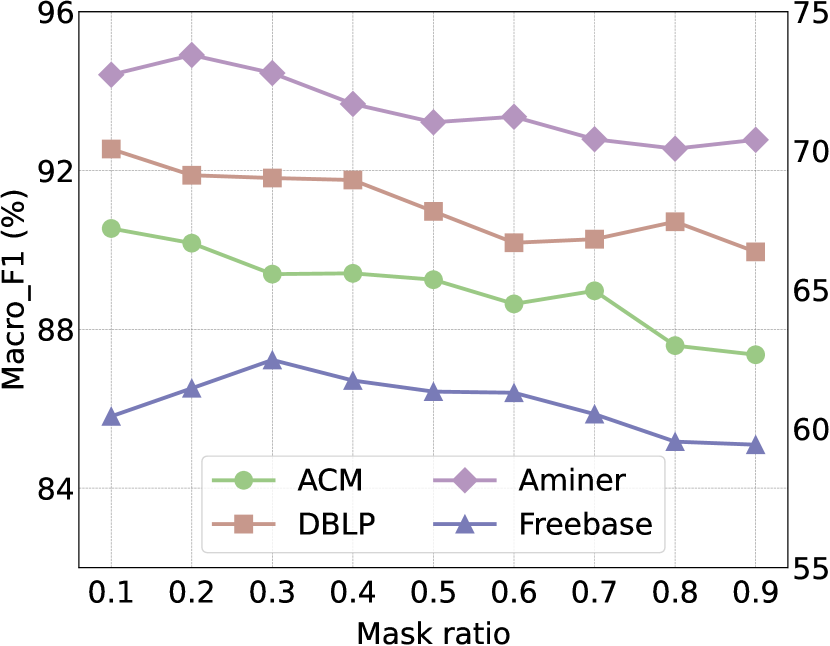
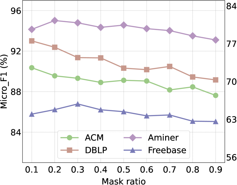
Mask ratio. In Section 4.2, we use a masked autoencoder, where the mask ratio plays a crucial role as a hyper-parameter in generating negative samples. As shown in Figure 8, our model typically achieves better results with a lower mask ratio, contrary to the conclusions drawn by HGMAE (Tian et al., 2023). We explain that, compared to generative feature reconstruction, the game between contrastive learning and generation learns to reconstruct the original data distribution by minimizing the distributional divergence rather than reconstructing individual samples (Liu et al., 2021).

In general, the findings suggest that higher inter-contrast, higher embedding dimensions, and lower mask ratios typically yield better results, with some dataset-specific variations.

6. Conclusion

In this paper, we propose a novel generative-contrastive heterogeneous graph neural network named GC-HGNN. It is a generative learning enhanced contrastive paradigm and a meaningful exploration. We combine meta-paths and masked autoencoders to create augmented contrastive views without disrupting the data structure. Then, we propose position-aware and semantic-aware sampling strategies to alleviate the synthesize hard negatives problem in heterogeneous graphs. Finally, we propose a hierarchical contrastive learning self-supervised framework to capture local and global information. In particular, the hierarchical contrastive learning and sampling strategies constitute the enhanced discriminator under this paradigm. Experiments demonstrate that this discriminator effectively improves the stability of output embeddings. The generative-contrastive framework significantly improves the performance of node classification and link prediction tasks. We compare our model with seventeen state-of-the-art models on eight real-world datasets. Our model outperforms the latest contrastive and generative baselines on multiple tasks.

References

- (1)
- Chen et al. (2023) Mengru Chen, Chao Huang, Lianghao Xia, Wei Wei, Yong Xu, and Ronghua Luo. 2023. Heterogeneous graph contrastive learning for recommendation. In Proceedings of the Sixteenth ACM International Conference on Web Search and Data Mining. 544–552.
- Chen et al. (2020) Ting Chen, Simon Kornblith, Mohammad Norouzi, and Geoffrey Hinton. 2020. A simple framework for contrastive learning of visual representations. In International conference on machine learning. PMLR, 1597–1607.
- Chowdhery et al. (2023) Aakanksha Chowdhery, Sharan Narang, Jacob Devlin, Maarten Bosma, Gaurav Mishra, Adam Roberts, Paul Barham, Hyung Won Chung, Charles Sutton, Sebastian Gehrmann, et al. 2023. Palm: Scaling language modeling with pathways. Journal of Machine Learning Research 24, 240 (2023), 1–113.
- Devlin et al. (2018) Jacob Devlin, Ming-Wei Chang, Kenton Lee, and Kristina Toutanova. 2018. Bert: Pre-training of deep bidirectional transformers for language understanding. arXiv preprint arXiv:1810.04805 (2018).
- Dong et al. (2017) Yuxiao Dong, Nitesh V Chawla, and Ananthram Swami. 2017. metapath2vec: Scalable representation learning for heterogeneous networks. In Proceedings of the 23rd ACM SIGKDD international conference on knowledge discovery and data mining. 135–144.
- Fu et al. (2020) Xinyu Fu, Jiani Zhang, Ziqiao Meng, and Irwin King. 2020. Magnn: Metapath aggregated graph neural network for heterogeneous graph embedding. In Proceedings of The Web Conference 2020. 2331–2341.
- Goodfellow et al. (2020) Ian Goodfellow, Jean Pouget-Abadie, Mehdi Mirza, Bing Xu, David Warde-Farley, Sherjil Ozair, Aaron Courville, and Yoshua Bengio. 2020. Generative adversarial networks. Commun. ACM 63, 11 (2020), 139–144.
- Grill et al. (2020) Jean-Bastien Grill, Florian Strub, Florent Altché, Corentin Tallec, Pierre Richemond, Elena Buchatskaya, Carl Doersch, Bernardo Avila Pires, Zhaohan Guo, Mohammad Gheshlaghi Azar, et al. 2020. Bootstrap your own latent-a new approach to self-supervised learning. Advances in neural information processing systems 33 (2020), 21271–21284.
- Han et al. (2022) Hui Han, Tianyu Zhao, Cheng Yang, Hongyi Zhang, Yaoqi Liu, Xiao Wang, and Chuan Shi. 2022. Openhgnn: an open source toolkit for heterogeneous graph neural network. In Proceedings of the 31st ACM International Conference on Information & Knowledge Management. 3993–3997.
- He et al. (2020b) Kaiming He, Haoqi Fan, Yuxin Wu, Saining Xie, and Ross Girshick. 2020b. Momentum contrast for unsupervised visual representation learning. In Proceedings of the IEEE/CVF conference on computer vision and pattern recognition. 9729–9738.
- He et al. (2020a) Xiangnan He, Kuan Deng, Xiang Wang, Yan Li, Yongdong Zhang, and Meng Wang. 2020a. Lightgcn: Simplifying and powering graph convolution network for recommendation. In Proceedings of the 43rd International ACM SIGIR conference on research and development in Information Retrieval. 639–648.
- Hou et al. (2022) Zhenyu Hou, Xiao Liu, Yukuo Cen, Yuxiao Dong, Hongxia Yang, Chunjie Wang, and Jie Tang. 2022. Graphmae: Self-supervised masked graph autoencoders. In Proceedings of the 28th ACM SIGKDD Conference on Knowledge Discovery and Data Mining. 594–604.
- Hu et al. (2020b) Ziniu Hu, Yuxiao Dong, Kuansan Wang, Kai-Wei Chang, and Yizhou Sun. 2020b. Gpt-gnn: Generative pre-training of graph neural networks. In Proceedings of the 26th ACM SIGKDD International Conference on Knowledge Discovery & Data Mining. 1857–1867.
- Hu et al. (2020a) Ziniu Hu, Yuxiao Dong, Kuansan Wang, and Yizhou Sun. 2020a. Heterogeneous graph transformer. In Proceedings of the web conference 2020. 2704–2710.
- Kalantidis et al. (2020) Yannis Kalantidis, Mert Bulent Sariyildiz, Noe Pion, Philippe Weinzaepfel, and Diane Larlus. 2020. Hard negative mixing for contrastive learning. Advances in neural information processing systems 33 (2020), 21798–21809.
- Lin et al. (2022) Zihan Lin, Changxin Tian, Yupeng Hou, and Wayne Xin Zhao. 2022. Improving graph collaborative filtering with neighborhood-enriched contrastive learning. In Proceedings of the ACM web conference 2022. 2320–2329.
- Liu et al. (2021) Xiao Liu, Fanjin Zhang, Zhenyu Hou, Li Mian, Zhaoyu Wang, Jing Zhang, and Jie Tang. 2021. Self-supervised learning: Generative or contrastive. IEEE transactions on knowledge and data engineering 35, 1 (2021), 857–876.
- Liu et al. (2023) Yue Liu, Xihong Yang, Sihang Zhou, Xinwang Liu, Zhen Wang, Ke Liang, Wenxuan Tu, Liang Li, Jingcan Duan, and Cancan Chen. 2023. Hard sample aware network for contrastive deep graph clustering. In Proceedings of the AAAI conference on artificial intelligence, Vol. 37. 8914–8922.
- Long et al. (2021) Xiaoling Long, Chao Huang, Yong Xu, Huance Xu, Peng Dai, Lianghao Xia, and Liefeng Bo. 2021. Social recommendation with self-supervised metagraph informax network. In Proceedings of the 30th ACM international conference on information & knowledge management. 1160–1169.
- Park et al. (2020) Chanyoung Park, Donghyun Kim, Jiawei Han, and Hwanjo Yu. 2020. Unsupervised attributed multiplex network embedding. In Proceedings of the AAAI Conference on Artificial Intelligence, Vol. 34. 5371–5378.
- Perozzi et al. (2014) Bryan Perozzi, Rami Al-Rfou, and Steven Skiena. 2014. Deepwalk: Online learning of social representations. In Proceedings of the 20th ACM SIGKDD international conference on Knowledge discovery and data mining. 701–710.
- Ren et al. (2019) Yuxiang Ren, Bo Liu, Chao Huang, Peng Dai, Liefeng Bo, and Jiawei Zhang. 2019. Heterogeneous deep graph infomax. arXiv preprint arXiv:1911.08538 (2019).
- Rendle et al. (2012) Steffen Rendle, Christoph Freudenthaler, Zeno Gantner, and Lars Schmidt-Thieme. 2012. BPR: Bayesian personalized ranking from implicit feedback. arXiv preprint arXiv:1205.2618 (2012).
- Schlichtkrull et al. (2018) Michael Schlichtkrull, Thomas N Kipf, Peter Bloem, Rianne Van Den Berg, Ivan Titov, and Max Welling. 2018. Modeling relational data with graph convolutional networks. In The Semantic Web: 15th International Conference, ESWC 2018, Heraklion, Crete, Greece, June 3–7, 2018, Proceedings 15. Springer, 593–607.
- Shi et al. (2018) Chuan Shi, Binbin Hu, Wayne Xin Zhao, and S Yu Philip. 2018. Heterogeneous information network embedding for recommendation. IEEE Transactions on Knowledge and Data Engineering 31, 2 (2018), 357–370.
- Sun and Han (2013) Yizhou Sun and Jiawei Han. 2013. Mining heterogeneous information networks: a structural analysis approach. Acm Sigkdd Explorations Newsletter 14, 2 (2013), 20–28.
- Sun et al. (2011) Yizhou Sun, Jiawei Han, Xifeng Yan, Philip S Yu, and Tianyi Wu. 2011. Pathsim: Meta path-based top-k similarity search in heterogeneous information networks. Proceedings of the VLDB Endowment 4, 11 (2011), 992–1003.
- Tian et al. (2023) Yijun Tian, Kaiwen Dong, Chunhui Zhang, Chuxu Zhang, and Nitesh V Chawla. 2023. Heterogeneous graph masked autoencoders. In Proceedings of the AAAI Conference on Artificial Intelligence, Vol. 37. 9997–10005.
- Van der Maaten and Hinton (2008) Laurens Van der Maaten and Geoffrey Hinton. 2008. Visualizing data using t-SNE. Journal of machine learning research 9, 11 (2008).
- Velickovic et al. (2017) Petar Velickovic, Guillem Cucurull, Arantxa Casanova, Adriana Romero, Pietro Lio, Yoshua Bengio, et al. 2017. Graph attention networks. stat 1050, 20 (2017), 10–48550.
- Wang et al. (2019) Xiao Wang, Houye Ji, Chuan Shi, Bai Wang, Yanfang Ye, Peng Cui, and Philip S Yu. 2019. Heterogeneous graph attention network. In The world wide web conference. 2022–2032.
- Wang et al. (2021) Xiao Wang, Nian Liu, Hui Han, and Chuan Shi. 2021. Self-supervised heterogeneous graph neural network with co-contrastive learning. In Proceedings of the 27th ACM SIGKDD conference on knowledge discovery & data mining. 1726–1736.
- Wang et al. (2023) Zehong Wang, Qi Li, Donghua Yu, Xiaolong Han, Xiao-Zhi Gao, and Shigen Shen. 2023. Heterogeneous graph contrastive multi-view learning. In Proceedings of the 2023 SIAM International Conference on Data Mining (SDM). SIAM, 136–144.
- Wu et al. (2023) Cheng Wu, Chaokun Wang, Jingcao Xu, Ziyang Liu, Kai Zheng, Xiaowei Wang, Yang Song, and Kun Gai. 2023. Graph Contrastive Learning with Generative Adversarial Network. In Proceedings of the 29th ACM SIGKDD Conference on Knowledge Discovery and Data Mining. 2721–2730.
- Wu et al. (2021) Jiancan Wu, Xiang Wang, Fuli Feng, Xiangnan He, Liang Chen, Jianxun Lian, and Xing Xie. 2021. Self-supervised graph learning for recommendation. In Proceedings of the 44th international ACM SIGIR conference on research and development in information retrieval. 726–735.
- Yang et al. (2023) Yonghui Yang, Zhengwei Wu, Le Wu, Kun Zhang, Richang Hong, Zhiqiang Zhang, Jun Zhou, and Meng Wang. 2023. Generative-contrastive graph learning for recommendation. In Proceedings of the 46th International ACM SIGIR Conference on Research and Development in Information Retrieval. 1117–1126.
- You et al. (2020) Yuning You, Tianlong Chen, Yongduo Sui, Ting Chen, Zhangyang Wang, and Yang Shen. 2020. Graph contrastive learning with augmentations. Advances in neural information processing systems 33 (2020), 5812–5823.
- Yu et al. (2022b) Le Yu, Leilei Sun, Bowen Du, Chuanren Liu, Weifeng Lv, and Hui Xiong. 2022b. Heterogeneous graph representation learning with relation awareness. IEEE Transactions on Knowledge and Data Engineering (2022).
- Yu et al. (2022a) Pengyang Yu, Chaofan Fu, Yanwei Yu, Chao Huang, Zhongying Zhao, and Junyu Dong. 2022a. Multiplex heterogeneous graph convolutional network. In Proceedings of the 28th ACM SIGKDD Conference on Knowledge Discovery and Data Mining. 2377–2387.
- Zhang et al. (2019) Chuxu Zhang, Dongjin Song, Chao Huang, Ananthram Swami, and Nitesh V Chawla. 2019. Heterogeneous graph neural network. In Proceedings of the 25th ACM SIGKDD international conference on knowledge discovery & data mining. 793–803.
- Zhang et al. (2023) Yi Zhang, Yiwen Zhang, Dengcheng Yan, Shuiguang Deng, and Yun Yang. 2023. Revisiting graph-based recommender systems from the perspective of variational auto-encoder. ACM Transactions on Information Systems 41, 3 (2023), 1–28.
- Zhang et al. (2024) Yi Zhang, Yiwen Zhang, Dengcheng Yan, Qiang He, and Yun Yang. 2024. NIE-GCN: Neighbor Item Embedding-Aware Graph Convolutional Network for Recommendation. IEEE Transactions on Systems, Man, and Cybernetics: Systems (2024).
- Zheng et al. (2021) Jiawei Zheng, Qianli Ma, Hao Gu, and Zhenjing Zheng. 2021. Multi-view denoising graph auto-encoders on heterogeneous information networks for cold-start recommendation. In Proceedings of the 27th ACM SIGKDD Conference on Knowledge Discovery & Data Mining. 2338–2348.
- Zhu et al. (2022) Yanqiao Zhu, Yichen Xu, Hejie Cui, Carl Yang, Qiang Liu, and Shu Wu. 2022. Structure-enhanced heterogeneous graph contrastive learning. In Proceedings of the 2022 SIAM International Conference on Data Mining (SDM). SIAM, 82–90.