Multi-Contact Inertial Estimation and Localization in Legged Robots

Abstract

Optimal estimation is a promising tool for multi-contact inertial estimation and localization. To harness its advantages in robotics, it is crucial to solve these large and challenging optimization problems efficiently. To tackle this, we (i) develop a multiple-shooting solver that exploits both temporal and parametric structures through a parametrized Riccati recursion. Additionally, we (ii) propose an inertial local manifold that ensures its full physical consistency. It also enhances convergence compared to the singularity-free log-Cholesky approach. To handle its singularities, we (iii) introduce a nullspace approach in our optimal estimation solver. We (iv) finally develop the analytical derivatives of contact dynamics for both inertial parametrizations. Our framework can successfully solve estimation problems for complex maneuvers such as brachiation in humanoids. We demonstrate its numerical capabilities across various robotics tasks and its benefits in experimental trials with the Go1 robot.

I Introduction

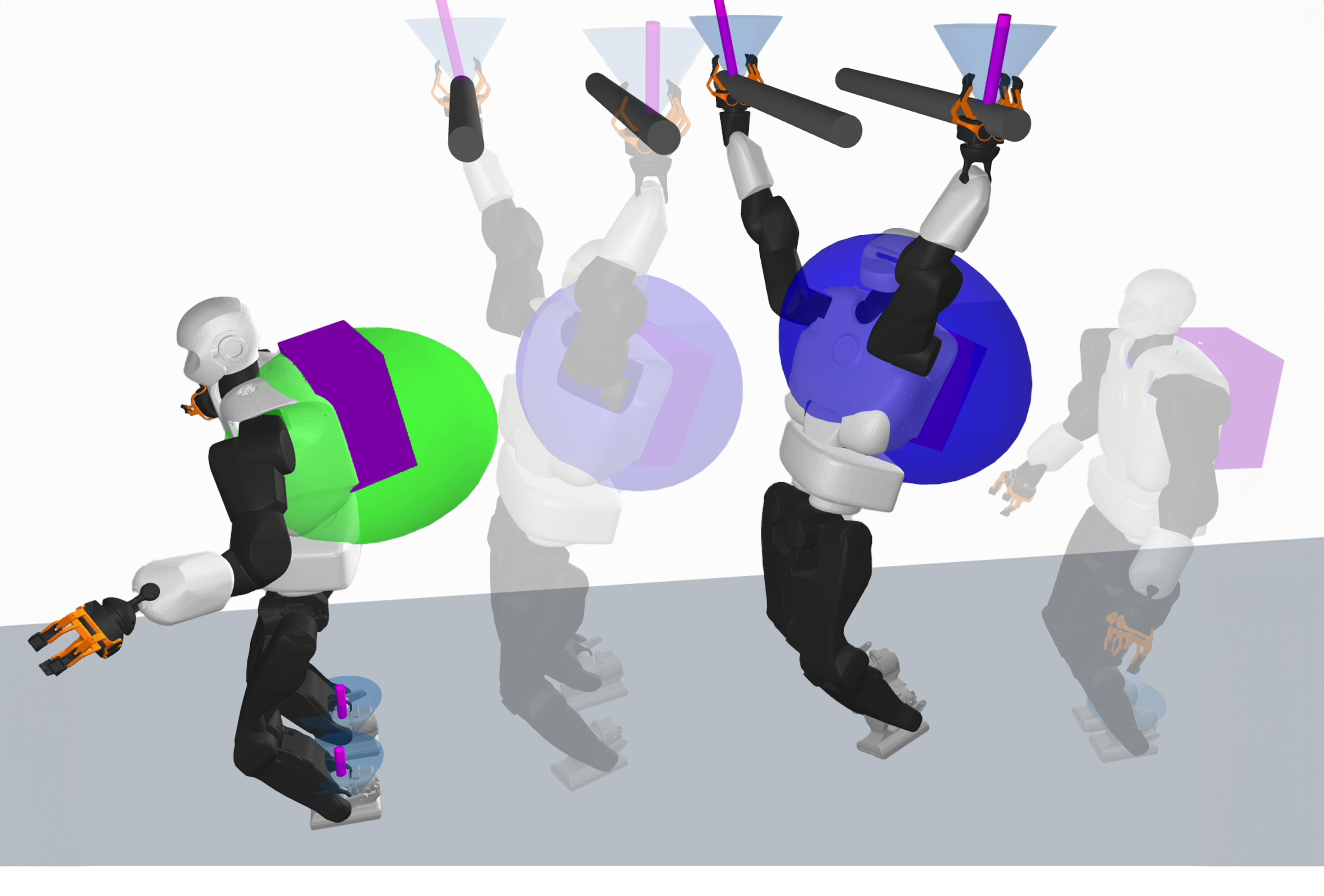
Optimal estimation (OE) [1] emerges as a powerful tool for interpreting observations and accurately estimating a system’s true state, including internal changes like unknown payloads. In the context of robotics, this framework takes into account both proprioceptive and exteroceptive observations [2, 3]. It systematically incorporates considerations such as robot dynamics and nonholonomics [4], balance conditions [5], and kinematic range. Its application in robotics holds promising potentials. For instance, it could empower humanoid robots to manipulate unknown objects or to execute agile maneuvers while carrying an unknown payload (Fig. 1).

Algorithms for optimal estimation solve variations of the following problem:

$$\min_{\mathbf{x}_{s},\mathbf{w}_{s},\boldsymbol{\theta}} \,\,\frac{1}{2}\|\mathbf{x}_{0}\ominus\mathbf{\bar{x}}_{0}\|^{2}_{\boldsymbol{\Sigma}_{\mathbf{x}_{0}}^{-1}}+\frac{1}{2}\|\boldsymbol{\theta}-\boldsymbol{\bar{\theta}}\|^{2}_{\boldsymbol{\Sigma}_{\boldsymbol{\theta}}^{-1}}$$

$$+\frac{1}{2}\sum_{k=0}^{N-1}\|\mathbf{w}_{k}\|^{2}_{\boldsymbol{\Sigma}_{\mathbf{w}_{N}}^{-1}}+\frac{1}{2}\sum_{k=1}^{N}\|\mathbf{\hat{z}}_{k}\ominus\mathbf{h}(\mathbf{x}_{k};\boldsymbol{\theta}|\mathbf{\hat{u}}_{k})\|^{2}_{\boldsymbol{\Sigma}_{\mathbf{z}_{k}}^{-1}}$$

$$\text{s.t.}\quad\mathbf{x}_{k+1}=\mathbf{f}(\mathbf{x}_{k};\boldsymbol{\theta}|\mathbf{\hat{u}}_{k})\oplus\mathbf{w}_{k},$$ (1)

where $\mathbf{x}\in\mathcal{X}\subseteq\mathbb{R}^{n_{x}}$ represents the system’s state, $\mathbf{w}\in\mathcal{T}_{\mathbf{x}}\mathcal{X}\subseteq\mathbb{R}^{n_{x}}$ describes its uncertainty, $\boldsymbol{\theta}\in\mathbb{R}^{n_{\theta}}$ are static parameters defining the system’s inertial properties, $\mathbf{\hat{u}}_{k}$ denotes the applied (and known) control commands, $\mathbf{\hat{z}}\in\mathcal{Z}\subseteq\mathbb{R}^{n_{z}}$ are observations, and $\mathbf{x}_{0}$ is the arrival state. Section I aims at finding the maximum a-posteriori estimate $P(\mathbf{x}_{s},\mathbf{w}_{s},\boldsymbol{\theta}|\mathbf{\hat{z}}_{s})$ as the state, parameters, uncertainties, and observations correspond to Gaussian distributions, i.e., $\mathbf{x}_{k}\thicksim\mathcal{N}(\mathbf{\bar{x}}_{k},\boldsymbol{\Sigma}_{\mathbf{x}_{k}})$, $\boldsymbol{\theta}\thicksim\mathcal{N}(\boldsymbol{\bar{\theta}},\boldsymbol{\Sigma}_{\boldsymbol{\theta}})$, $\mathbf{w}_{k}\thicksim\mathcal{N}(\mathbf{0},\boldsymbol{\Sigma}_{\mathbf{w}_{k}})$, and $\mathbf{\hat{z}}_{k}\thicksim\mathcal{N}(\mathbf{0},\boldsymbol{\Sigma}_{\mathbf{z}_{k}})$, respectively. The term $\frac{1}{2}\|\mathbf{x}_{0}\ominus\mathbf{\bar{x}}_{0}\|^{2}_{\boldsymbol{\Sigma}_{\mathbf{x}_{0}}^{-1}}$ describes the arrival cost, where $\ominus$ is the difference operator used to optimize over state manifolds [6, 7, 8]. Additionally, the term $\frac{1}{2}\|\boldsymbol{\theta}-\boldsymbol{\bar{\theta}}\|^{2}_{\boldsymbol{\Sigma}_{\boldsymbol{\theta}}^{-1}}$ specifies the uncertainties in the system’s parameters. Finally, $\mathbf{f}:\mathcal{X}\times\mathbb{R}^{n_{\theta}}\to\mathcal{T}_{\mathbf{x}}\mathcal{X}$ and $\mathbf{h}:\mathcal{X}\times\mathbb{R}^{n_{\theta}}\to\mathcal{Z}$ are nonlinear functions describing the system dynamics and measurements.

Figure 1: Talos executing intricate monkey bar maneuvers with an unidentified payload. In the initial stages, our estimator meticulously pinpoints Talos’ localization and estimates its payload’s properties: mass, barycenter, and rotational inertia. The ellipsoid’s dimensions, position, radius, and color serve as visual indicators, representing estimations of the payload’s mass, barycenter, principal components of inertia, and algorithm convergence. To watch the video, click the picture or see https://youtu.be/J4pqAU7O8Ew.

I-A Related work

To address optimal estimation in robotics, one can leverage well-established direct methods [9], which transcribes Section I into a nonlinear programming (NLP) problem. Direct methods involve the discretization of both state and uncertainties, followed by optimization using sparse general-purpose NLP software such as Snopt [10], Knitro [11], and Ipopt [12]. These software rely on sparse linear solvers such as MA27, MA57, and MA97 (see [13]) to factorize the large Karush-Kuhn-Tucker (KKT) problem. However, a limitation of these linear solvers is their inefficiency in exploiting the Markovian structure of OE problems [14], restricting their applicability in real-time applications, especially in legged robotics. These computational limitations are attributed to their difficulties in utilizing data cache accesses efficiently, resulting in the exclusion of OE strategies. Indeed, recent works focused on factor graphs formulations [15, 16, 17] are restricted to localization approaches only while ignoring the robot’s dynamics. In contrast, our approach considers the robot’s dynamics, thereby reducing drift errors in proprioceptive localization.

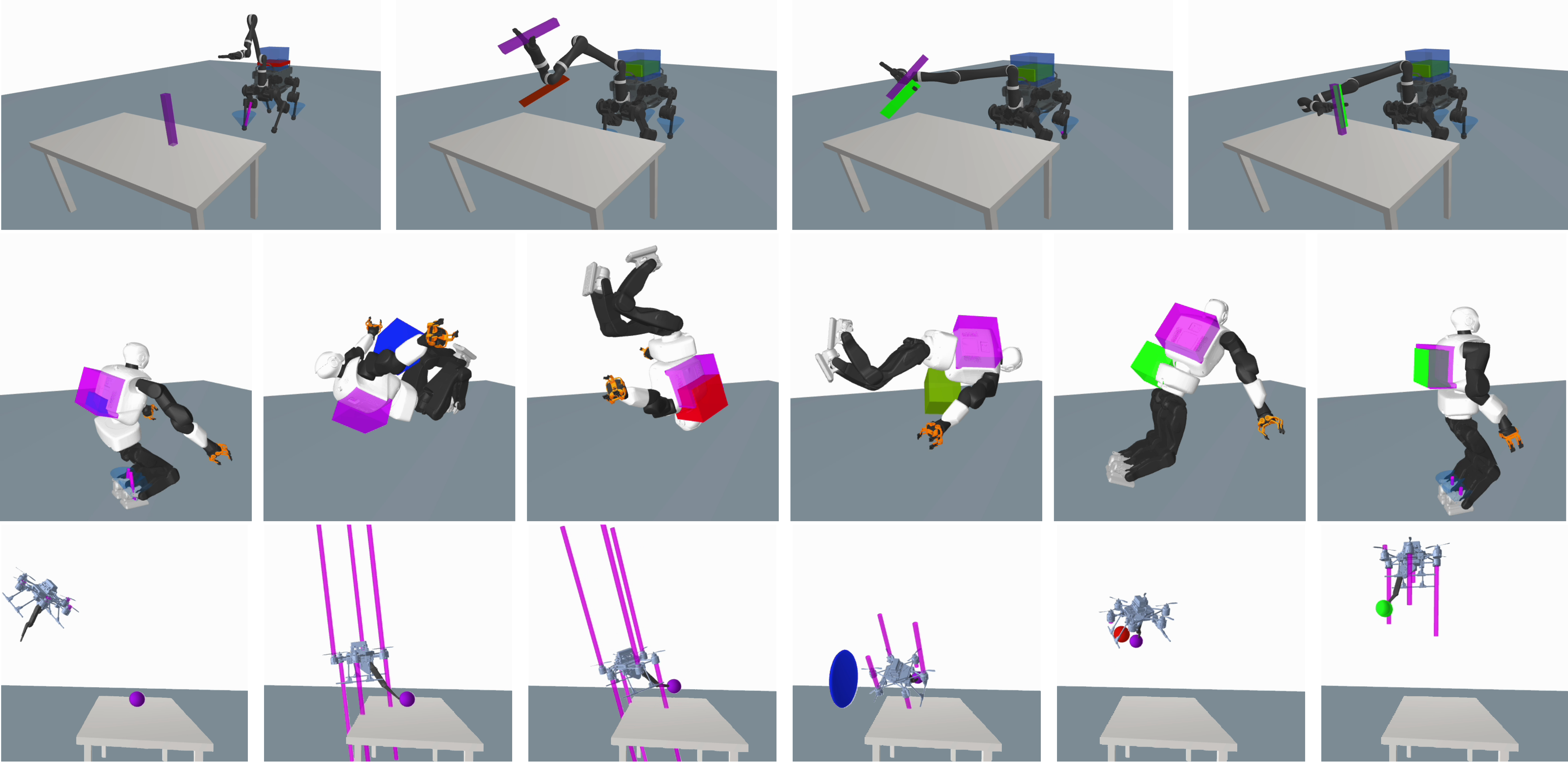
Figure 2: Snapshots illustrating simulated online multi-contact inertial estimation and localization. (top) ANYmal with a Kinova arm carries an unknown payload while grasping an unknown object. (middle) Talos performs a backflip while simultaneously estimating its backpack. (bottom) Borinot grasping an sphere with a symmetric inertia (only converges thanks to the null-space parametrization). Unknown payloads are represented in magenda, and upon convergence of the estimator, the estimated payload is depicted in green. To watch the video, click the picture or see https://youtu.be/J4pqAU7O8Ew.

Alternatively, we can leverage Bellman’s principle of optimality [18] to break the optimal estimation problem into a sequence of smaller subproblems. This approach effectively exploits the Markovian structure, resulting in a differential dynamic programming (DDP) approach for optimal estimation [19]. Additionally, by augmenting the system’s state with its internal parameters, or parametrizing the dynamics, we can simultaneously solve identification and localization problems via DDP [20]. However, these DDP approaches, being single shooting algorithms, are prone to numerical instability and require a good initialization [9], both crucial considerations for their application in robotics. These numerical instabilities, arise from enforcing dynamic feasibility, can be mitigated through feasibility-driven methods [14, 21] or multiple shooting strategies [22, 23] as proposed in model predictive control (MPC) literature. Moreover, DDP approaches for optimal estimation presuppose knowledge of the arrival state, a condition not attainable in real-world applications. In contrast, our framework incorporates the arrival state estimation.

To estimate inertial parameters in robotics, two key aspects must be leveraged: (i) the affine relationship between these parameters and the generalized torques, as initially developed in [24], and (ii) the analytical derivatives of rigid body algorithms [25, 26]. The second aspect is particularly relevant to us, as the derivatives of forward dynamics in [25] rely on the inertial matrix method (IMM) outlined in [27]. This is because IMMs involve Cholesky decompositions of the joint-space inertia matrix, limiting their operation to inertial parameters that are fully physically consistent.

Conditions for full physical consistency boils down to triangle inequality constraints [28]. However, numerical optimization guarantees inequality feasibilities at convergence, limiting its application to IMMs. Alternatively, these conditions can be embedded in a smooth manifold defined via a log-Cholesky parametrization [29]. This manifold, being singularity-free, exhibits highly nonlinear geometry. Nevetheless, it is possible to build a smoother manifold by developing an OE solver that handles these singularities. These ideas lead us to a novel exponential eigenvalue local manifold, with a better convergence rate, coupled with a nullspace resolution (Fig. 2).

I-B Contribution

Our main contribution is an efficient approach for solving hybrid optimal estimation problems in inertial estimation and localization. It relies on four technical contributions:

1. a novel smooth manifold with local submersion that guarantees full physical consistency of inertial parameters,

2. an algorithm for analytical derivatives of the hybrid contact dynamics regarding the inertial parameters,

3. a nullspace approach for handling singularities encountered in inertial identification, and

4. a multiple-shooting algorithm for parametrized DDP with hybrid contact dynamics.

Our optimal estimation framework is the first of its class, even when considering the log-Cholesky parametrization (see Fig. 2 and https://youtu.be/J4pqAU7O8Ew). This is because previous work [29] focuses solely on inertial identification. Additionally, it relies on a novel multiple-shooting solver that combines nullspace parametrization to handle the exponential-eigenvalue singularities. Such singularities occur when the principal components of inertia at barycenter are the same, as in a solid sphere or a disk with uniform density.

II Background

In this section, we provide an introduction to contact dynamics, inertial parameters, and the conditions for their full physical consistency.

II-A Contact dynamics

The dynamics of rigid body systems, subject to contact constraints at the acceleration level, are governed by:

$$\mathbf{M}(\mathbf{q})\mathbf{\dot{v}} =\boldsymbol{\tau}(\mathbf{u})-\mathbf{h}(\mathbf{q},\mathbf{v})+\mathbf{J}_{c}(\mathbf{q})^{\intercal}\boldsymbol{\lambda}_{c},$$ (2)

$$\mathbf{J}_{c}(\mathbf{q})\mathbf{\dot{v}} =-\mathbf{a}_{c}(\mathbf{q},\mathbf{v}),$$ (3)

where $\mathbf{q}\in\mathcal{Q}\subseteq\mathbb{R}^{{n_{q}}}$, $\mathbf{v}\in\mathcal{T}_{\mathbf{q}}\mathcal{Q}\subseteq\mathbb{R}^{{n_{q}}}$, $\mathbf{u}\in\mathbb{R}^{{n_{u}}}$, and $\boldsymbol{\lambda}_{c}\in\mathbb{R}^{n_{c}}$ represent the configuration point, generalized velocity, control commands, and contact forces, respectively. The functions $\mathbf{M}:\mathcal{Q}\to\mathbb{R}^{{n_{q}}\times{n_{q}}}$ represents the joint-space inertia matrix, $\boldsymbol{\tau}:\mathbb{R}^{n_{u}}\to\mathbb{R}^{n_{q}}$ denotes the joint-generalized torque, $\mathbf{J}_{c}:\mathcal{T}_{\mathbf{q}}\mathcal{Q}\to\mathbb{R}^{{n_{c}}\times{n_{q}}}$ is the contact Jacobian, and $\mathbf{h}:\mathcal{Q}\times\mathcal{T}_{\mathbf{q}}\mathcal{Q}\to\mathbb{R}^{n_{q}}$ is a force vector containing the Coriolis, centrifugal and gravitational terms. In the absence of contacts, free dynamics are governed by Eq. 2 with $\boldsymbol{\lambda}_{c}=\mathbf{0}$.

Free dynamics are frequently computed using the articulated body algorithm (ABA) [27]. In contrast, contact dynamics are commonly computed using a Schur-complement approach based on the IMM [30]. Moreover, analytical derivatives of contact dynamics with respect to $\mathbf{q}$, $\mathbf{v}$ and $\boldsymbol{\tau}$ are computed based on the algorithms described in [25], as explained in [7].

II-B Inertial parameters of rigid bodies

The spatial inertia of a rigid body $i$, encapsulating the body’s mass-density field $\rho:\mathbb{R}^{3}\to\mathbb{R}_{\geq 0}$, can be defined using a vector $\boldsymbol{\pi}_{i}\in\mathbb{R}^{10}$, whose elements are

$$\boldsymbol{\pi}_{i}=\begin{bmatrix}m&h_{x}&h_{y}&h_{z}&I_{xx}&I_{xy}&I_{yy}&I_{xz}&I_{yz}&I_{zz}\end{bmatrix}^{\intercal},$$ (4)

where $m\in\mathbb{R}$ denotes the body’s mass, $\mathbf{h}=[h_{x}\,\,h_{y}\,\,h_{z}]^{\intercal}=m\mathbf{c}\in\mathbb{R}^{3}$ represents the first mass moment with $\mathbf{c}$ as its barycenter, and $[I_{xx}\,\,I_{xy}\,\,I_{yy}\,\,I_{xz}\,\,I_{yz}\,\,I_{zz}]^{\intercal}$ are the elements of its inertia matrix $\mathbf{I}\in\mathbb{R}^{3\times 3}$. Both barycenter and rotational inertia are expressed in the body-fixed reference frame as introduced in [24]. Moreover, the rotational inertia $\mathbf{I}$ can be expressed at the barycenter using the parallel axis theorem:

$$\mathbf{I}_{c}=\mathbf{I}-\frac{\mathbf{S}(\mathbf{h})\mathbf{S}(\mathbf{h})^{\intercal}}{m},$$ (5)

where $\mathbf{S}:\mathbb{R}^{3}\to\mathfrak{s0}(3)$ is the skew-symmetric matrix, also known as the Lie algebra of $SO(3)$ (see [8]).

As described in [24], the generalized torques can be expressed as an affine function of the inertial parameters $\boldsymbol{\pi}$, i.e.,

$$\boldsymbol{\tau}(\mathbf{u})=\mathbf{Y}(\mathbf{q},\mathbf{v},\mathbf{\dot{v}})\boldsymbol{\pi},$$ (6)

where $\mathbf{Y}:\mathcal{Q}\times\mathcal{T}_{\mathbf{q}}\mathcal{Q}\times\mathcal{T}_{\mathbf{q}}\mathcal{Q}\to\mathbb{R}^{{n_{q}}\times 10{n_{b}}}$ is the joint-torque regressor matrix with ${n_{b}}$ as the number of rigid bodies.

II-C Physically-consistent spatial inertia

We say that $\boldsymbol{\pi}_{i}$ is fully physically consistent, or $\boldsymbol{\pi}_{i}\in\mathcal{I}$, if there exists a finite-value density function $\rho$. The set $\mathcal{I}\subset\mathbb{R}^{10}$ is characterized by the following inequality constraints:

$$\begin{aligned} m\geq 0,\quad&\mathbf{I}_{c}\succeq 0,\\ D_{x}<D_{y}+D_{z},\quad D_{y}<D_{x}+&D_{z},\quad D_{z}<D_{x}+D_{y}.\end{aligned}$$ (7)

Here, $\mathbf{D}=\text{diag}(D_{x},D_{y},D_{z})\in\mathbb{R}^{3\times 3}$ represents the principal moments of inertia, computed as $\mathbf{I}_{c}=\mathbf{R}\mathbf{D}\mathbf{R}^{\intercal}$ with $\mathbf{R}\in SO(3)$. The condition $\mathbf{I}_{c}\succeq 0$ ensures positivity in the principal components of inertia, and the triangle inequalities enforce positivity in second moments of mass [28].

The rotational inertia $\mathbf{I}_{c}$ can be interpreted as a point-mass distribution with covariance $\boldsymbol{\Sigma}_{c}$. When mapping this to its spatial inertia, it results in a 4x4 pseudo-inertia matrix [31] given by:

$$\mathbf{J}=\begin{bmatrix}\boldsymbol{\Sigma}&\mathbf{h}\\ \mathbf{h}^{\intercal}&m\end{bmatrix},\quad\text{where}\quad\boldsymbol{\Sigma}=\frac{1}{2}\text{Tr}(\mathbf{I})\mathbf{1}_{3}-\mathbf{I},$$ (8)

$\boldsymbol{\Sigma}=\boldsymbol{\Sigma}_{c}+m\mathbf{c}\mathbf{c}^{\intercal}$, $\text{Tr}(\cdot)$ is the trace operator, and $\mathbf{1}_{3}$ is a 3x3 identity matrix. The pseudo-inertia matrix $\mathbf{J}\in\mathcal{S}_{++}^{4}$ must satisfy the condition $\mathbf{J}\succeq 0$ for full physical consistency.

III Parametrization of inertial parameters

To map parameters $\boldsymbol{\theta}\in\mathbb{R}^{10}$ to fully physically consistent parameters $\boldsymbol{\pi}_{i}\in\mathcal{I}$, we can construct a smooth isomorphic mapping $\boldsymbol{\psi}:\mathbb{R}^{10}\to\mathcal{I}$. Below, we introduce the log-Cholesky parametrization and then proceed to develop our exponential eigenvalue parametrization.

III-A Log-Cholesky parametrization

Log-Cholesky decompositions are applicable to semidefine matrices, enabling us to encode the condition $\mathbf{J}_{i}\succeq 0$ for physical consistency of body $i$. As suggested in [29], a log-Cholesky parametrization of the pseudo inertia $\mathbf{J}=\mathbf{U}\mathbf{U}^{\intercal}$, with

$$\mathbf{U}=e^{\alpha}\begin{bmatrix}e^{{d_{1}}}&{s_{12}}&{s_{13}}&{t_{1}}\\ 0&e^{{d_{2}}}&{s_{23}}&{t_{2}}\\ 0&0&{s_{23}}&{t_{3}}\\ 0&0&0&1\end{bmatrix},$$ (9)

can be employed to establish an isomorphic map $\boldsymbol{\pi}=\boldsymbol{\psi}(\boldsymbol{\theta}_{\text{lchol}})$. Here, $\boldsymbol{\psi}\coloneqq\text{vech}(\mathbf{U}\mathbf{U}^{\intercal})$, where the vech operator denotes the serialization operation of $\mathbf{J}$, and

$$\boldsymbol{\theta}_{\text{lchol}}=\begin{bmatrix}\alpha&{d_{1}}&{d_{2}}&{d_{3}}&{s_{12}}&{s_{23}}&{s_{13}}&{t_{1}}&{t_{2}}&{t_{3}}\end{bmatrix}^{\intercal}\in\mathbb{R}^{10}.$$ (10)

III-B Exponential eigenvalue parametrization

The singular value decomposition of $\mathbf{I}_{c}$ can be expressed in terms of its second moments of mass:

$$\mathbf{I}_{c}=\mathbf{R}\,\text{diag}\left(\mathbf{P}\mathbf{L}\right)\mathbf{R}^{\intercal},\,\,\text{where}\,\,\mathbf{P}=\begin{bmatrix}0&1&1\\ 1&0&1\\ 1&1&0\end{bmatrix}$$ (11)

and $\mathbf{L}=[L_{x}\,\,L_{y}\,\,L_{z}]\in\mathbb{R}^{3}_{\geq 0}$ denotes the second moments of mass. Ensuring positivity in $L_{x}$, $L_{y}$, $L_{z}$ is equivalent to satisfying both $\mathbf{I}_{c}\succeq 0$ and the triangle inequalities in Eq. 7. Intuitively, these conditions on $L_{x}$, $L_{y}$, $L_{z}$, and $m\geq 0$ can be embedded using an exponential map. Formally, their manifold constraints are

$$\text{diag}(\mathbf{L})\cdot\text{diag}(\mathbf{L})^{-1}=\mathbf{1}_{3},\quad m\cdot m^{-1}=1,$$ (12)

defining the real numbers as their Lie algebra structure. Therefore, our parametrization is given by

$$m=\text{exp}(\sigma_{m}),\quad\mathbf{L}=\begin{bmatrix}\text{exp}(\sigma_{x})&\text{exp}(\sigma_{y})&\text{exp}(\sigma_{z})\end{bmatrix}^{\intercal},$$ (13)

where $\sigma_{m}$ and $(\sigma_{x},\sigma_{y},\sigma_{z})$ denote the mass and rotational inertia parameters, respectively. Moreover, the structure of the rotational matrix $\mathbf{R}$ is guaranteed by parametrizing it via the Lie algebra of $SO(3)$, i.e.,

$$\mathbf{R}=\text{Exp}(\boldsymbol{\omega}),$$ (14)

where $\boldsymbol{\omega}=[\omega_{x}\,\,\omega_{y}\,\,\omega_{z}]\in\mathbb{R}^{3}\cong\mathfrak{s0}(3)$, and $\text{Exp}:\mathbb{R}^{3}\to SO(3)$ converts this vector elements to the elements of the $SO(3)$ group. Moreover, we obtain the inertia $\mathbf{I}$ via Eq. 5.

Combining the exponential maps and stacking them into a vector, we construct a map with local submersion $\boldsymbol{\pi}=\boldsymbol{\psi}(\boldsymbol{\theta}_{\text{eeval}})$, where

$$\boldsymbol{\theta}_{\text{eeval}}=\begin{bmatrix}\sigma_{m}&h_{x}&h_{y}&h_{z}&\omega_{x}&\omega_{y}&\omega_{z}&\sigma_{x}&\sigma_{y}&\sigma_{z}\end{bmatrix}^{\intercal}\in\mathbb{R}^{10}.$$ (15)

Finally, we can analytically compute $\frac{\partial\boldsymbol{\pi}}{\partial\boldsymbol{\theta}}$ for both $\boldsymbol{\theta}_{\text{lchol}}$ and $\boldsymbol{\theta}_{\text{eeval}}$, as they are smooth and differentiable parametrizations.

IV Multi-contact optimal estimation

Optimal estimation with hybrid events involves the use of multiphase dynamics and reset maps:

$$\min_{\mathbf{x}_{s},\mathbf{w}_{s},\boldsymbol{\theta}} \ell_{N}(\mathbf{x}_{N};\boldsymbol{\theta}|\mathbf{\hat{z}}_{N})+\sum_{k=0}^{N-1}\ell_{k}(\mathbf{x}_{k},\mathbf{w}_{k};\boldsymbol{\theta}|\mathbf{\hat{z}}_{k})$$ (16)

s.t. for $$p\in\mathcal{P}$$:

for $$k\in\{p_{0},p_{0}+1,\cdots,p_{N}-1\}$$:

$$\hskip 8.00003pt\mathbf{x}_{k+1}=\mathbf{f}_{p}(\mathbf{x}_{k};\boldsymbol{\theta}|\mathbf{\hat{u}}_{k})\oplus\mathbf{w}_{k}$$ (phase dyn.)

$$\mathbf{x}_{p_{N+1}}=\boldsymbol{\Delta}_{p}(\mathbf{x}_{p_{N}};\boldsymbol{\theta}),$$ (reset map)

where $\mathbf{f}_{p}:\mathcal{X}\times\mathbb{R}^{n_{\theta}}\to\mathcal{T}_{\mathbf{x}}\mathcal{X}$ describes the contact dynamics in phase $p$, and $\boldsymbol{\Delta}_{p}:\mathcal{X}\times\mathbb{R}^{n_{\theta}}\to\mathcal{T}_{\mathbf{x}}\mathcal{X}$ defines its contact-gain transition (modelled via impulse dynamics). Below, we develop their analytical derivatives w.r.t. $\boldsymbol{\theta}$. For their analytical derivatives w.r.t. $\mathbf{x}=(\mathbf{q},\mathbf{v})$, we refer to [7, 32].

IV-A Analytical derivatives of parametrized dynamics

In free dynamics, inertial parameters $\boldsymbol{\pi}$ exhibit a linear relationship with the generalized torques. Additionally, the property $\partial\text{FD}=\mathbf{M}^{-1}\partial\text{ID}$ holds, given that the forward dynamics (FD) is the reciprocal of inverse dynamics (ID) [25]. Therefore, by applying the chain rule, we compute the analytical derivatives of forward dynamics with respect to $\boldsymbol{\theta}$ as

$$\frac{\partial\text{FD}}{\partial\boldsymbol{\theta}}=\mathbf{M}(\mathbf{q})^{-1}\frac{\partial\text{ID}}{\partial\boldsymbol{\pi}}\frac{\partial\boldsymbol{\pi}}{\partial\boldsymbol{\theta}}=\mathbf{M}(\mathbf{q})^{-1}\mathbf{Y}(\mathbf{q},\mathbf{v},\mathbf{\dot{v}})\frac{\partial\boldsymbol{\pi}}{\partial\boldsymbol{\theta}}.$$ (17)

Moving on to contact dynamics, and similarly to [7], we apply the chain rule to derive the analytical derivatives for both the system’s acceleration and the contact forces:

$$\frac{\partial}{\partial\boldsymbol{\theta}}\begin{bmatrix}\mathbf{\dot{v}}\\ -\boldsymbol{\lambda}_{c}\end{bmatrix}=-\begin{bmatrix}\mathbf{M}(\mathbf{q})&\mathbf{J}_{c}(\mathbf{q})^{\intercal}\\ \mathbf{J}_{c}(\mathbf{q})&\mathbf{0}\end{bmatrix}^{-1}\begin{bmatrix}\frac{\partial\boldsymbol{\tau}}{\partial\boldsymbol{\theta}}\\ \mathbf{0}\end{bmatrix},$$ (18)

where $\frac{\partial\boldsymbol{\tau}}{\partial\boldsymbol{\theta}}=\mathbf{Y}(\mathbf{q},\mathbf{v},\mathbf{\dot{v}})\frac{\partial\boldsymbol{\pi}}{\partial\boldsymbol{\theta}}$. To enhance efficiency, this matrix inversion is performed via its Schur complement. This complement requires computing $\mathbf{M}^{-1}$. Similar to free dynamics, we achieve this through the Cholesky decomposition of $\mathbf{M}$, an approach typically employed in IMMs. Moreover, these matrix inversions are computed for derivatives with respect to $\mathbf{q}$ and $\mathbf{v}$, allowing for the reuse of computations and leveraging sparsity in Eq. 18.

Similarly, derivatives of impulse dynamics [7] involves inverting the same matrix but with:

$$\begin{aligned} \frac{\partial\boldsymbol{\tau}}{\partial\boldsymbol{\theta}}&\coloneqq\left(\frac{\partial\text{ID}(\mathbf{q},\mathbf{0},\mathbf{v}^{+}-\mathbf{v})}{\partial\boldsymbol{\pi}}-\frac{\partial\text{ID}(\mathbf{q},\mathbf{0},\mathbf{0})}{\partial\boldsymbol{\pi}}\right)\frac{\partial\boldsymbol{\pi}}{\partial\boldsymbol{\theta}},\\ &=\left(\mathbf{Y}(\mathbf{q},\mathbf{0},\mathbf{v}^{+}-\mathbf{v})-\mathbf{Y}(\mathbf{q},\mathbf{0},\mathbf{0})\right)\frac{\partial\boldsymbol{\pi}}{\partial\boldsymbol{\theta}},\end{aligned}$$ (19)

where $\mathbf{v}^{+}\in\mathcal{T}_{\mathbf{q}}\mathcal{Q}\subseteq\mathbb{R}^{{n_{q}}}$ is the post impact velocity.

V DDP with parametrized dynamics

Handling parametrized dynamics requires to introduce additional decision variables $\boldsymbol{\theta}$. To exploit its temporal structure, we begin by examining the optimality conditions through the lens of Bellman, ultimately leading to a parametrized Riccati recursion.

V-A Optimality conditions

By examining the Bellman equation of Eq. 16, specifically,

$$\begin{aligned} \mathcal{V}\left(\mathbf{x};\boldsymbol{\theta}\right|\mathbf{\hat{u}},\mathbf{\hat{z}})=&\min_{\mathbf{x}^{\prime},\mathbf{x},\mathbf{w};\boldsymbol{\theta}}\ell(\mathbf{x},\mathbf{w};\boldsymbol{\theta}|\mathbf{\hat{z}})+\mathcal{V}^{\prime}(\mathbf{x}^{\prime};\boldsymbol{\theta}|\mathbf{\hat{u}},\mathbf{\hat{z}})\\ &\quad\text{s.t.}\quad\mathbf{x}^{\prime}=\mathbf{f}(\mathbf{x},\mathbf{w};\boldsymbol{\theta}|\mathbf{\hat{u}}),\end{aligned}$$ (20)

we break the optimal estimation problem into a sequence of subproblems. The KKT point for each subproblem can be efficiently determined using the Newton method, yielding the following linear system of equations in each iteration:

$$\begin{bmatrix}\mathcal{L}_{\mathbf{x}\mathbf{x}}&\mathcal{L}_{\mathbf{x}\mathbf{w}}&\mathcal{L}_{\mathbf{x}\boldsymbol{\theta}}&\mathbf{f}_{\mathbf{x}}^{\intercal}&\\ \mathcal{L}_{\mathbf{x}\mathbf{w}}^{\intercal}&\mathcal{L}_{\mathbf{w}\mathbf{w}}&\mathcal{L}_{\mathbf{w}\boldsymbol{\theta}}&\mathbf{f}_{\mathbf{w}}^{\intercal}&\\ \mathcal{L}_{\mathbf{x}\boldsymbol{\theta}}^{\intercal}&\mathcal{L}_{\mathbf{w}\boldsymbol{\theta}}^{\intercal}&\mathcal{L}_{\boldsymbol{\theta}\boldsymbol{\theta}}&\mathbf{f}_{\boldsymbol{\theta}}^{\intercal}&\mathcal{V}_{\mathbf{x}\boldsymbol{\theta}}^{\prime\intercal}\\ \mathbf{f}_{\mathbf{x}}&\mathbf{f}_{\mathbf{w}}&\mathbf{f}_{\boldsymbol{\theta}}&&-\mathbf{I}\\ &&\mathcal{V}_{\mathbf{x}\boldsymbol{\theta}}^{\prime}&-\mathbf{I}&\mathcal{V}_{\mathbf{x}\mathbf{x}}^{\prime}\end{bmatrix}\begin{bmatrix}\delta\mathbf{x}\\ \delta\mathbf{w}\\ \delta\boldsymbol{\theta}\\ \boldsymbol{\xi}^{\mathbf{+}}\\ \delta\mathbf{x}^{\prime}\end{bmatrix}=-\begin{bmatrix}\boldsymbol{\ell}_{\mathbf{x}}\\ \boldsymbol{\ell}_{\mathbf{w}}\\ \boldsymbol{\ell}_{\boldsymbol{\theta}}+\mathcal{V}_{\boldsymbol{\theta}}^{\prime}\\ \mathbf{\bar{f}}\\ \mathcal{V}_{\mathbf{x}}^{\prime}\end{bmatrix}$$

with: (21)

$$\hskip 5.0pt\boldsymbol{\xi}^{\mathbf{+}}\coloneqq\boldsymbol{\xi}+\delta\boldsymbol{\xi},\hskip 58.0001pt\mathbf{\bar{f}}\coloneqq\mathbf{f}(\mathbf{x},\mathbf{w};\boldsymbol{\theta})\ominus\mathbf{x}^{\prime},$$

$$\hskip 5.0pt\mathcal{L}_{\mathbf{x}\mathbf{x}}\coloneqq\boldsymbol{\ell}_{\mathbf{x}\mathbf{x}}+\mathcal{V}_{\mathbf{x}}^{\prime}\cdot\mathbf{f}_{\mathbf{x}\mathbf{x}},\hskip 20.00003pt\mathcal{L}_{\mathbf{x}\mathbf{w}}\coloneqq\boldsymbol{\ell}_{\mathbf{x}\mathbf{w}}+\mathcal{V}_{\mathbf{x}}^{\prime}\cdot\mathbf{f}_{\mathbf{x}\mathbf{w}},$$

$$\hskip 5.0pt\mathcal{L}_{\mathbf{x}\boldsymbol{\theta}}\coloneqq\boldsymbol{\ell}_{\mathbf{x}\boldsymbol{\theta}}+\mathcal{V}_{\mathbf{x}}^{\prime}\cdot\mathbf{f}_{\mathbf{x}\boldsymbol{\theta}},\hskip 20.00003pt\mathcal{L}_{\mathbf{w}\mathbf{w}}\coloneqq\boldsymbol{\ell}_{\mathbf{w}\mathbf{w}}+\mathcal{V}_{\mathbf{x}}^{\prime}\cdot\mathbf{f}_{\mathbf{w}\mathbf{w}},$$

$$\hskip 5.0pt\mathcal{L}_{\mathbf{w}\boldsymbol{\theta}}\coloneqq\boldsymbol{\ell}_{\mathbf{w}\boldsymbol{\theta}}+\mathcal{V}_{\mathbf{x}}^{\prime}\cdot\mathbf{f}_{\mathbf{w}\boldsymbol{\theta}},\hskip 15.00002pt\mathcal{L}_{\boldsymbol{\theta}\boldsymbol{\theta}}\coloneqq\boldsymbol{\ell}_{\boldsymbol{\theta}\boldsymbol{\theta}}+\mathcal{V}_{\boldsymbol{\theta}\boldsymbol{\theta}}^{\prime}+\mathcal{V}_{\mathbf{x}}^{\prime}\cdot\mathbf{f}_{\boldsymbol{\theta}\boldsymbol{\theta}}.$$

Here, $\boldsymbol{\ell}_{\mathbf{p}}$, $\mathbf{f}_{\mathbf{p}}$, are the first derivative of the cost and the system dynamics with respect to $\mathbf{p}$, with $\mathbf{p}$ a hypothetical decision variable that represents $\mathbf{x}$, $\mathbf{w}$ or $\boldsymbol{\theta}$; $\boldsymbol{\ell}_{\mathbf{p}\mathbf{p}}$, $\mathbf{f}_{\mathbf{p}\mathbf{p}}$ are the second derivatives; $\mathcal{V}_{\mathbf{p}}^{\prime}$ is the gradient of the value function; $\mathcal{V}_{\mathbf{p}\mathbf{p}}^{\prime}$ is the Hessian of the value function; $\mathbf{\bar{f}}$ describe the gaps or infeasibility in the dynamics; $\delta\mathbf{x}$, $\delta\mathbf{w}$, $\delta\boldsymbol{\theta}$, $\delta\mathbf{x}^{\prime}$ and $\delta\boldsymbol{\xi}$ provides the search direction computed for the primal and dual variables, respectively; and the prime superscript is used to refer to the next node.

Similar to optimal control [14, Section 2.2], we observe the presence of the Markovian structure, leading to $\boldsymbol{\xi}^{\mathbf{+}}=\mathcal{V}_{\mathbf{x}}^{\prime}+\begin{bmatrix}\mathcal{V}_{\mathbf{x}\mathbf{x}}^{\prime}&\mathcal{V}_{\mathbf{x}\boldsymbol{\theta}}^{\prime}\end{bmatrix}\begin{bmatrix}\delta\mathbf{x}^{\prime}\\ \delta\boldsymbol{\theta}\end{bmatrix}$. This establishes a connection between the KKT conditions with the Pontryagin’s maximum principle [18] because $\boldsymbol{\xi}^{\mathbf{+}}$ assumes the role of the next costate. This connection becomes evident when augmenting the system’s state with its internal parameters, contributing to the condensation of the system of equations in Section V-A into:

$$\begin{bmatrix}\mathbf{Q}_{\mathbf{x}\mathbf{x}}&\mathbf{Q}_{\mathbf{x}\mathbf{w}}&\mathbf{Q}_{\mathbf{x}\boldsymbol{\theta}}\\ \mathbf{Q}_{\mathbf{x}\mathbf{w}}^{\intercal}&\mathbf{Q}_{\mathbf{w}\mathbf{w}}&\mathbf{Q}_{\mathbf{w}\boldsymbol{\theta}}\\ \mathbf{Q}_{\mathbf{x}\boldsymbol{\theta}}^{\intercal}&\mathbf{Q}_{\mathbf{w}\boldsymbol{\theta}}^{\intercal}&\mathbf{Q}_{\boldsymbol{\theta}\boldsymbol{\theta}}\end{bmatrix}\begin{bmatrix}\delta\mathbf{x}\\ \delta\mathbf{w}\\ \delta\boldsymbol{\theta}\end{bmatrix}=-\begin{bmatrix}\mathbf{Q}_{\mathbf{x}}\\ \mathbf{Q}_{\mathbf{w}}\\ \mathbf{Q}_{\boldsymbol{\theta}}\end{bmatrix},$$ (22)

where the $\mathbf{Q}$’s terms represent the local approximation of the action-value function whose expressions are:

$$\small\mathbf{Q}_{\mathbf{x}\mathbf{x}}=\mathcal{L}_{\mathbf{x}\mathbf{x}}+\mathbf{f}_{\mathbf{x}}^{\intercal}\mathcal{V}_{\mathbf{x}\mathbf{x}}^{\prime}\mathbf{f}_{\mathbf{x}},\hskip 18.90009pt\mathbf{Q}_{\mathbf{w}\boldsymbol{\theta}}=\mathcal{L}_{\mathbf{w}\boldsymbol{\theta}}+\mathbf{f}_{\mathbf{w}}^{\intercal}(\mathcal{V}_{\mathbf{x}\boldsymbol{\theta}}^{\prime}+\mathcal{V}_{\mathbf{x}\mathbf{x}}^{\prime}\mathbf{f}_{\boldsymbol{\theta}}),$$

$$\small\mathbf{Q}_{\mathbf{x}\mathbf{w}}=\mathcal{L}_{\mathbf{x}\mathbf{w}}+\mathbf{f}_{\mathbf{x}}^{\intercal}\mathcal{V}_{\mathbf{x}\mathbf{x}}^{\prime}\mathbf{f}_{\mathbf{w}},\hskip 15.29999pt\mathbf{Q}_{\mathbf{x}\boldsymbol{\theta}}=\mathcal{L}_{\mathbf{x}\boldsymbol{\theta}}+\mathbf{f}_{\mathbf{x}}^{\intercal}(\mathcal{V}_{\mathbf{x}\boldsymbol{\theta}}^{\prime}+\mathcal{V}_{\mathbf{x}\mathbf{x}}^{\prime}\mathbf{f}_{\boldsymbol{\theta}}),$$

$$\small\mathbf{Q}_{\mathbf{w}\mathbf{w}}=\mathcal{L}_{\mathbf{w}\mathbf{w}}+\mathbf{f}_{\mathbf{w}}^{\intercal}\mathcal{V}_{\mathbf{x}\mathbf{x}}^{\prime}\mathbf{f}_{\mathbf{w}},\hskip 10.79999pt\mathbf{Q}_{\boldsymbol{\theta}\boldsymbol{\theta}}=\mathcal{L}_{\boldsymbol{\theta}\boldsymbol{\theta}}+\mathbf{f}_{\boldsymbol{\theta}}^{\intercal}(2\mathcal{V}_{\mathbf{x}\boldsymbol{\theta}}^{\prime}+\mathcal{V}_{\mathbf{x}\mathbf{x}}^{\prime}\mathbf{f}_{\boldsymbol{\theta}}),$$

$$\small\mathbf{Q}_{\mathbf{x}}=\boldsymbol{\ell}_{\mathbf{x}}+\mathbf{f}_{\mathbf{x}}^{\intercal}\mathcal{V}_{\mathbf{x}}^{+},\hskip 44.1pt\mathbf{Q}_{\boldsymbol{\theta}}=\boldsymbol{\ell}_{\boldsymbol{\theta}}+\mathcal{V}_{\boldsymbol{\theta}}^{+}+\mathbf{f}_{\boldsymbol{\theta}}^{\intercal}\mathcal{V}_{\mathbf{x}}^{+},$$

$$\small\mathbf{Q}_{\mathbf{w}}=\boldsymbol{\ell}_{\mathbf{w}}+\mathbf{f}_{\mathbf{w}}^{\intercal}\mathcal{V}_{\mathbf{x}}^{+}$$ (23)

with $\mathcal{V}_{\mathbf{x}}^{+}\coloneqq\mathcal{V}_{\mathbf{x}}^{\prime}+\mathcal{V}_{\mathbf{x}\mathbf{x}}^{\prime}\mathbf{\bar{f}}$ and $\mathcal{V}_{\boldsymbol{\theta}}^{+}\coloneqq\mathcal{V}_{\boldsymbol{\theta}}^{\prime}+\mathcal{V}_{\mathbf{x}\boldsymbol{\theta}}^{\prime}\mathbf{\bar{f}}$ as the gradients of the value function after the deflection produced by the dynamics infeasibility $\mathbf{\bar{f}}$ (see [7]). To exploit the parametric structure, we then compute the estimation policy and value function as functions of the parameters and arrival state.

V-B Policy and value function

The system of linear equations in Eq. 22 can be interpreted as a quadratic program that locally minimizes the Bellman equation Eq. 20, i.e.,

$$\delta\mathcal{V}(\delta\mathbf{x};\delta\boldsymbol{\theta}|\mathbf{\hat{u}},\mathbf{\hat{z}}) \simeq$$ (24)

$$\min_{\delta\mathbf{w}}\frac{1}{2}\begin{bmatrix}1\\ \delta\mathbf{x}\\ \delta\mathbf{w}\\ \delta\boldsymbol{\theta}\end{bmatrix}^{\intercal}\begin{bmatrix}&\mathbf{Q}_{\mathbf{x}}^{\intercal}&\mathbf{Q}_{\mathbf{w}}^{\intercal}&\mathbf{Q}_{\boldsymbol{\theta}}^{\intercal}\\ \mathbf{Q}_{\mathbf{x}}&\mathbf{Q}_{\mathbf{x}\mathbf{x}}&\mathbf{Q}_{\mathbf{x}\mathbf{w}}&\mathbf{Q}_{\mathbf{x}\boldsymbol{\theta}}\\ \mathbf{Q}_{\mathbf{w}}&\mathbf{Q}_{\mathbf{x}\mathbf{w}}^{\intercal}&\mathbf{Q}_{\mathbf{w}\mathbf{w}}&\mathbf{Q}_{\mathbf{w}\boldsymbol{\theta}}\\ \mathbf{Q}_{\boldsymbol{\theta}}&\mathbf{Q}_{\mathbf{x}\boldsymbol{\theta}}^{\intercal}&\mathbf{Q}_{\mathbf{w}\boldsymbol{\theta}}^{\intercal}&\mathbf{Q}_{\boldsymbol{\theta}\boldsymbol{\theta}}\end{bmatrix}\begin{bmatrix}1\\ \delta\mathbf{x}\\ \delta\mathbf{w}\\ \delta\boldsymbol{\theta}\end{bmatrix}.$$

This leads to what we call the DDP approach for optimal estimation. The term is chosen because it computes the changes in the estimation policy $\delta\mathbf{w}$ as a function of changes in the system’s state $\delta\mathbf{x}$ and its internal parameters $\delta\boldsymbol{\theta}$ given observations $(\mathbf{\hat{u}},\mathbf{\hat{z}})$, i.e.,

$$\delta\mathbf{w}=-\mathbf{k}-\mathbf{K}\delta\textbf{x}-\mathbf{P}\delta\boldsymbol{\theta},$$ (25)

where $\mathbf{k}=\mathbf{Q}_{\mathbf{w}\mathbf{w}}^{-1}\mathbf{Q}_{\mathbf{w}}$, $\mathbf{K}=\mathbf{Q}_{\mathbf{w}\mathbf{w}}^{-1}\mathbf{Q}_{\mathbf{x}\mathbf{w}}^{\intercal}$ and $\mathbf{P}=\mathbf{Q}_{\mathbf{w}\mathbf{w}}^{-1}\mathbf{Q}_{\mathbf{w}\boldsymbol{\theta}}$ are the feed-forward and feedback terms. In this approach, when plugging the changes in the estimation into Eq. 24, we obtain a quadratic approximation of the optimal arrival cost (a.k.a. value function) as follows

$$\delta\mathcal{V}(\delta\mathbf{x};\delta\boldsymbol{\theta}|\mathbf{\hat{u}},\mathbf{\hat{z}}) \simeq\Delta\mathcal{V}_{1}+\frac{\Delta\mathcal{V}_{2}}{2}$$

$$+\frac{1}{2}\begin{bmatrix}\delta\mathbf{x}\\ \delta\boldsymbol{\theta}\end{bmatrix}^{\intercal}\begin{bmatrix}\mathcal{V}_{\mathbf{x}\mathbf{x}}&\mathcal{V}_{\mathbf{x}\boldsymbol{\theta}}\\ \mathcal{V}_{\mathbf{x}\boldsymbol{\theta}}^{\intercal}&\mathcal{V}_{\boldsymbol{\theta}\boldsymbol{\theta}}\end{bmatrix}\begin{bmatrix}\delta\mathbf{x}\\ \delta\boldsymbol{\theta}\end{bmatrix}+\begin{bmatrix}\mathcal{V}_{\mathbf{x}}\\ \mathcal{V}_{\boldsymbol{\theta}}\end{bmatrix}^{\intercal}\begin{bmatrix}\delta\mathbf{x}\\ \delta\boldsymbol{\theta}\end{bmatrix},$$ (26)

where

$$\Delta\mathcal{V}_{1}=-\mathbf{k}^{\intercal}\mathbf{Q}_{\mathbf{w}},\quad\quad\quad\,\,\Delta\mathcal{V}_{2}=\mathbf{k}^{\intercal}\mathbf{Q}_{\mathbf{w}\mathbf{w}}\mathbf{k},$$

$$\mathcal{V}_{\mathbf{x}}=\mathbf{Q}_{\mathbf{x}}-\mathbf{Q}_{\mathbf{x}\mathbf{w}}\mathbf{k},\quad\quad\,\mathcal{V}_{\boldsymbol{\theta}}=\mathbf{Q}_{\boldsymbol{\theta}}-\mathbf{Q}_{\mathbf{w}\boldsymbol{\theta}}^{\intercal}\mathbf{k},$$

$$\mathcal{V}_{\mathbf{x}\mathbf{x}}=\mathbf{Q}_{\mathbf{x}\mathbf{x}}-\mathbf{Q}_{\mathbf{x}\mathbf{w}}\mathbf{K},\quad\mathcal{V}_{\boldsymbol{\theta}\boldsymbol{\theta}}=\mathbf{Q}_{\boldsymbol{\theta}\boldsymbol{\theta}}-\mathbf{Q}_{\mathbf{w}\boldsymbol{\theta}}^{\intercal}\mathbf{P},$$

$$\mathcal{V}_{\mathbf{x}\boldsymbol{\theta}}=\mathbf{Q}_{\mathbf{x}\boldsymbol{\theta}}-\mathbf{Q}_{\mathbf{x}\mathbf{w}}\mathbf{P},$$ (27)

and $\mathbf{Q}_{\mathbf{x}\mathbf{w}}\mathbf{P}=\mathbf{K}^{\intercal}\mathbf{Q}_{\mathbf{w}\boldsymbol{\theta}}$.

The derivations of changes in the optimal policy and value function are expressed in terms of the search direction for the system’s parameters $\delta\boldsymbol{\theta}$ and the arrival state $\delta\mathbf{x}_{0}$. To compute the search directions $\delta\boldsymbol{\theta}$ and $\delta\mathbf{x}_{0}$, we analyze the conditions of optimality for the initial node as follows.

V-C Arrival state and parameters

By substituting Eq. 25 into the condensed KKT equations of the initial or arrival node in Eq. 22, we obtain:

$$\begin{bmatrix}\mathcal{V}_{\mathbf{x}\mathbf{x}}^{\bullet}&\mathcal{V}_{\mathbf{x}\boldsymbol{\theta}}^{\bullet}\\ \mathcal{V}_{\mathbf{x}\boldsymbol{\theta}}^{\bullet\,\intercal}&\mathcal{V}_{\boldsymbol{\theta}\boldsymbol{\theta}}^{\bullet}\end{bmatrix}\begin{bmatrix}\delta\mathbf{x}_{0}\\ \delta\boldsymbol{\theta}\end{bmatrix}=-\begin{bmatrix}\mathcal{V}_{\mathbf{x}}^{\bullet}\\ \mathcal{V}_{\boldsymbol{\theta}}^{\bullet}\end{bmatrix},$$ (28)

where the bullet superscript is used to refer to the arrival node (e.g., $\delta\mathbf{x}_{0}\coloneqq\delta\mathbf{x}^{\bullet}$).

V-C1 Schur-complement

We can compute both $\delta\boldsymbol{\theta}$ and $\delta\mathbf{x}_{0}$ by factorizing Eq. 28 via the Schur-complement approach. This results in the following expressions:

$$\begin{array}[]{l}\delta\boldsymbol{\theta}=-\mathbf{k}_{\boldsymbol{\theta}}-\mathbf{K}_{\boldsymbol{\theta}}\delta\mathbf{x}_{0},\quad\delta\mathbf{x}_{0}\coloneqq-\mathcal{V}_{\mathbf{x}\mathbf{x}_{0}}^{-1}\mathcal{V}_{\mathbf{x}_{0}},\end{array}$$ (30)

where $\mathbf{k}_{\boldsymbol{\theta}}=\mathcal{V}_{\boldsymbol{\theta}\boldsymbol{\theta}}^{\bullet\,-1}\mathcal{V}_{\boldsymbol{\theta}}^{\bullet}$, $\mathbf{K}_{\boldsymbol{\theta}}=\mathcal{V}_{\boldsymbol{\theta}\boldsymbol{\theta}}^{\bullet\,-1}\mathcal{V}_{\mathbf{x}\boldsymbol{\theta}}^{\bullet\,\intercal}$ are the feed-forward and feedback terms of the parameters update,

$$\begin{array}[]{l}\mathcal{V}_{\mathbf{x}_{0}}=\mathcal{V}_{\mathbf{x}}^{\bullet}-\mathcal{V}_{\mathbf{x}\boldsymbol{\theta}}^{\bullet}\mathbf{k}_{\boldsymbol{\theta}},\quad\mathcal{V}_{\mathbf{x}\mathbf{x}_{0}}=\mathcal{V}_{\mathbf{x}\mathbf{x}}^{\bullet}-\mathcal{V}_{\mathbf{x}\boldsymbol{\theta}}^{\bullet}\mathbf{K}_{\boldsymbol{\theta}},\end{array}$$ (32)

are the derivatives of the value function associated to arrival node after updating the system’s parameters, and $\mathcal{V}_{\mathbf{x}\mathbf{x}_{0}}$ is of the Schur complement of Eq. 28. Now, we can rewrite the changes of the estimation policy as $\delta\mathbf{w}=-\mathbf{\bar{k}}-\mathbf{K}\delta\mathbf{x}$, where $\mathbf{\bar{k}}=\mathbf{k}+\mathbf{P}\delta\boldsymbol{\theta}$ represents the entire feed-forward term.

V-C2 Nullspace

Additionally, we can parametrize the search direction for the parameters as $\delta\boldsymbol{\theta}=\mathbf{Y}\delta\boldsymbol{\theta}_{\mathbf{y}}+\mathbf{Z}\delta\boldsymbol{\theta}_{\mathbf{z}}$. Here, $\mathbf{Z}\in\mathbb{R}^{{n_{\theta}}\times n_{z}}$ is the nullspace basis of $\mathcal{V}_{\boldsymbol{\theta}\boldsymbol{\theta}}^{\bullet}$ and $\mathbf{Y}\in\mathbb{R}^{{n_{\theta}}\times n_{y}}$ is its orthogonal matrix. Then, by substituting this parametrization into the second term of Eq. 30 and observing that $\mathcal{V}_{\boldsymbol{\theta}\boldsymbol{\theta}}^{\bullet}\mathbf{Z}=\mathbf{0}$, we obtain

$$\mathbf{Y}^{\intercal}\mathcal{V}_{\boldsymbol{\theta}\boldsymbol{\theta}}^{\bullet}\mathbf{Y}\delta\boldsymbol{\theta}_{\mathbf{y}}=-\overbrace{\mathbf{Y}^{\intercal}\mathcal{V}_{\boldsymbol{\theta}}^{\bullet}}^{\mathbf{k}_{\boldsymbol{\theta}\mathbf{y}}}-\overbrace{\mathbf{Y}^{\intercal}\mathcal{V}_{\mathbf{x}\boldsymbol{\theta}}^{\bullet\,\intercal}}^{\mathbf{K}_{\boldsymbol{\theta}\mathbf{y}}}\delta\mathbf{x}_{0},$$ (33)

where we pre-multiply by $\mathbf{Y}^{\intercal}$ to ensure the squareness of $\mathcal{V}_{\boldsymbol{\theta}\boldsymbol{\theta}}\mathbf{Y}$. Eq. 33 is then solved efficiently using a Cholesky decomposition. Finally, we recover the search direction for the parameters as $\delta\boldsymbol{\theta}=\mathbf{Y}\delta\boldsymbol{\theta}_{\mathbf{y}}$. Note that we compute $\delta\mathbf{x}_{0}$ as in the second term of Eq. 30.

V-D Forward rollouts

The search directions obtained from Eqs. 25, 30 and 33 provide updates for the system’s uncertainties, parameters, and arrival state. To determine the step length along these directions, we perfom a forward rollout of the disturbed system’s dynamics and evaluate the associated costs with the a-posteriori estimate. Below, we develop two distinct approaches inspired by optimal control literature, known as feasibility-driven and multiple shooting. Let’s start by describing how we update the arrival state and parameters first.

V-D1 Arrival state and parameters update

We follow a line-search approach for updating the arrival state and system’s parameters, i.e.,

$$\mathbf{x}_{0}^{\mathbf{+}}=\mathbf{x}_{0}\oplus\alpha\delta\mathbf{x}_{0},\quad\boldsymbol{\theta}^{\mathbf{+}}=\boldsymbol{\theta}+\alpha\delta\boldsymbol{\theta},$$ (34)

where $\alpha\in(0,1]$ denotes the step length and the plus superscript is used to denote the next guess under evaluation. Next, we begin by describing our feasibility-driven approach.

V-D2 Feasibility-driven rollout

Building upon classical line-search procedures (see [33, Chapter 3]), this approach tries the search direction along a feasibility-driven nonlinear rollout that preserves the gaps in the linear-dynamics sense [7]:

$$\begin{aligned} \mathbf{\bar{f}}_{k+1}^{\mathbf{+}}&=(\alpha-1)\mathbf{\bar{f}}_{k+1},\\ \mathbf{w}_{k}^{\mathbf{+}}&=\mathbf{w}_{k}-\alpha\mathbf{\bar{k}}_{k}-\mathbf{K}_{k}\delta\mathbf{x}_{k}^{\mathbf{+}},\\ \mathbf{x}_{k+1}^{\mathbf{+}}&=\mathbf{f}(\mathbf{x}_{k}^{\mathbf{+}},\mathbf{w}_{k}^{\mathbf{+}};\boldsymbol{\theta}^{\mathbf{+}})\oplus\mathbf{\bar{f}}_{k+1}^{\mathbf{+}},\end{aligned}$$ (35)

for $k=\{0,\dotsc,N\}\in\mathbb{N}$ and $\delta\mathbf{x}_{k}^{\mathbf{+}}=\mathbf{x}_{k}^{\mathbf{+}}\ominus\mathbf{x}_{k}$, where we employ backtracking procedure, and $\mathbf{x}_{k}^{+}$, $\mathbf{w}_{k}^{+}$ represent the new guesses, for the states and uncertainties, under evaluation.

V-D3 Multiple shooting rollout

Taking inspiration from multiple shooting approaches in optimal control, this approach tries a linear rollout and updates the gaps based on nonlinear shoots, i.e.,

$$\begin{aligned} \mathbf{w}_{k}^{\mathbf{+}}&=\mathbf{w}_{k}+\alpha\delta\mathbf{w}_{k},\\ \mathbf{x}_{k+1}^{\mathbf{+}}&=\mathbf{x}_{k+1}\oplus\alpha\delta\mathbf{x}_{k+1},\\ \mathbf{\bar{f}}_{k+1}^{\mathbf{+}}&=\mathbf{f}(\mathbf{x}_{k}^{\mathbf{+}},\mathbf{w}_{k}^{\mathbf{+}};\boldsymbol{\theta}_{k}^{\mathbf{+}})\ominus\mathbf{x}_{k+1}^{\mathbf{+}},\end{aligned}$$ (36)

for $k=\{0,\dotsc,N\}\in\mathbb{N}$. Compared to the feasibility-driven rollout in Eq. 35, multiple shooting rollouts can be broken into two parallel for loops: one for the update of the uncertainties and state, and another one for the update of the dynamics infeasibilities and costs. Below, we describe how we evaluate the goodness of a given step length $\alpha$.

V-E Merit function

Our merit function computes the expected cost reduction as a local approximation of the value function while being aware of the dynamics infeasibilities, i.e.,

$$\Delta\ell(\alpha)=\alpha\left(\Delta\mathcal{V}_{1}^{\boldsymbol{\theta}}+\frac{1}{2}\alpha\Delta\mathcal{V}_{2}^{\boldsymbol{\theta}}+\sum_{k=0}^{N-1}\left(\Delta\ell_{1_{k}}+\frac{1}{2}\alpha\Delta\ell_{2_{k}}\right)\right),$$ (37)

where, by considering that derivatives of the value function are deflected by the dynamics gaps, we have:

$$\Delta\ell_{1_{k}} =\Delta\mathcal{V}_{1_{k}}+\mathbf{\bar{f}}_{k}^{\intercal}\mathcal{V}_{\mathbf{x}_{k}},\quad\Delta\ell_{2_{k}}=\Delta\mathcal{V}_{2_{k}}+\mathbf{\bar{f}}_{k}^{\intercal}\mathcal{V}_{\mathbf{x}{\mathbf{x}_{k}}}\mathbf{\bar{f}}_{k},$$ (38)

with $\mathbf{\bar{f}}_{0}=\delta\mathbf{x}_{0}$, $\Delta\mathcal{V}_{1}^{\boldsymbol{\theta}}=\delta\boldsymbol{\theta}^{\intercal}\mathcal{V}_{\boldsymbol{\theta}}^{\bullet}$, and $\Delta\mathcal{V}_{2}^{\boldsymbol{\theta}}=2\,\mathbf{\bar{f}}_{0}^{\intercal}\mathcal{V}_{\mathbf{x}{\boldsymbol{\theta}}}^{\bullet}\delta\boldsymbol{\theta}+\delta\boldsymbol{\theta}\mathcal{V}_{\boldsymbol{\theta}{\boldsymbol{\theta}}}^{\bullet}\delta\boldsymbol{\theta}$. It is noteworthy that Eq. 37 simplies to the expected improvement formulation presented in [20], which employs a single shooting approach for optimal estimation.

We then compute a merit function of the form:

$$\phi(\mathbf{x}_{s},\mathbf{w}_{s},\boldsymbol{\theta};\nu) =$$

$$\ell(\mathbf{x}_{N};\boldsymbol{\theta})+\sum_{k=0}^{N-1}\ell(\mathbf{x}_{k},\mathbf{w}_{k};\boldsymbol{\theta})+\nu\epsilon(\mathbf{x}_{k},\mathbf{w}_{k};\boldsymbol{\theta}),$$ (39)

with $\epsilon(\mathbf{x}_{k},\mathbf{w}_{k};\boldsymbol{\theta})\coloneqq\|\mathbf{\bar{f}}_{k}\|_{1}$ measures the dynamics infeasibility of the current guess and

$$\nu\leftarrow\max\left(\beta^{\nu}\nu,\frac{\Delta\ell(1)}{(1-\rho)\sum_{k=0}^{N-1}\epsilon(\mathbf{x}_{k},\mathbf{w}_{k};\boldsymbol{\theta})}\right),$$ (40)

is a penalty parameter that balances optimality and feasibility, where $0<\rho<1$ is a tunable hyper-parameter and $\beta^{\nu}$ is a factor used to reduce $\nu$. The updating rule in Eq. 40 is inspired by [34, 21]. Finally, we utilize (1) a nonmonotone step acceptance strategy based on Armijo conditions and (2) a Levenberg-Marquardt scheme, similar to [21].

VI Results

We evaluate our multi-contact inertial estimation and localization framework through the following steps. First, we compare the numerical performance of both inertial parametrizations. Second, we analyze the effect of shooting approaches in optimal estimation. Third, we experimentally validate the advantages of updating inertial parameters for carrying unknown payloads. Finally, we show the importance of using hybrid dynamics for localization in legged robots. Additionally, we refer the reader to the video, where the performance of the null-space is evaluated.

VI-A Log-Cholesky vs Exponential Eigenvalue

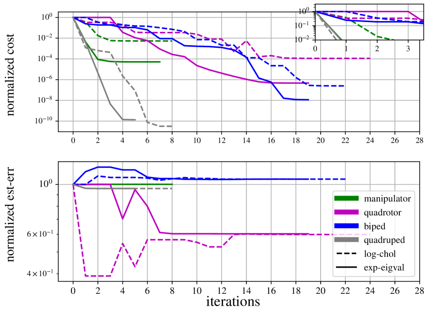
Our numerical performance analysis encompasses four diverse robotics systems: the Kinova arm, an asymmetric quadrotor, the ANYmal quadruped, and the Talos biped. In each scenario, we generated dynamically-consistent trajectories. This simulated encoders and IMU data (linear acceleration, gyroscopic velocities, and orientations) were integrated into the observation model, denote as $\mathbf{\hat{z}}=\mathbf{h}(\mathbf{x};\boldsymbol{\theta}|\mathbf{\hat{u}})$. Covariances for each observation, including the applied control $\mathbf{\hat{u}}$ for prediction, were meticously considered. To ensure a fair comparison between the inertial parameterizations, we omitted the parameter regularization term $\|\boldsymbol{\theta}-\boldsymbol{\bar{\theta}}\|^{2}_{\boldsymbol{\Sigma}_{\boldsymbol{\theta}}^{-1}}$. Moreover, we initialized the optimal estimators’ inertial parameters for all the bodies with the same error of $70\%$. Finally, we configured the estimators with a feasibility-driven rollout.

Figure 3: Top: Local convergence for both parametrizations, showing better convergence the exponential-eigenvalue (exp-eigval) parametrization in all cases. Bottom: Evolution of the estimation error, computed as the $\ell_{1}$-norm of difference between the optimized trajectory and the nominal one. Both parametrizations converge to the same local minima.

In each scenario illustrated in Fig. 3, both parametrization converge to the same estimated trajectory, resulting in the same estimation error. Nevertheless, the exponential eigenvalue parametrization demonstrated superior performance, characterized by faster convergence rates and often lower cost values. This can be attributed to its lower degree of nonlinearity compared to the log-Cholesky parametrization. Furthermore, the exponential eigenvalue parametrization offers a direct physical interpretation, proving advantageous, especially when partial knowledge of the rotational inertial is available. This interpretability facilitated easy tuning of lower covariances in known inertial parameters, contributing to enhanced precision and applicability in practical trials with the Go1 robot.

VI-B Numerical effect of rollout strategies

To evaluate the numerical impact of our feasibility-driven and multiple shooting rollouts, we randomly generated $100$ initial guess and compared their convergence, cost and estimation error against single shooting approaches. In Table I, we observe that multiple shooting rollouts reduced the costs or estimation errors across all cases. Moreover, single shooting rollouts have a reduced basin of attraction to local minima and can encounter difficulties in convergence for challenging cases.

TABLE I: Rollout’s local convergence computed from $100$ randomly initial guesses on three robotics systems.

		Iterations	Cost $[\cdot 10^{-1}]$	Error [$\ell_{\infty}$-norm]
Kinova	single	$39.7\pm 11.2$	$2.78\pm 0.89$	$3.11\pm 0.56$
	feasible	$\mathbf{44.7\pm 11.6}$	$1.16\pm 0.42$	$3.12\pm 0.01$
	multiple	$99.4\pm 71.5$	$\mathbf{0.61\pm 0.42}$	$\mathbf{2.67\pm 0.06}$
Quadrotor	single	$140.9\pm 65.1$	$0.12\pm 0.04$	$10.74\pm 0.0023$
	feasible	$150.1\pm 59.3$	$0.26\pm 0.11$	$10.74\pm 0.0013$
	multiple	$\mathbf{16.9\pm 19.1}$	$\mathbf{0.07\pm 1.31}$	$\mathbf{10.74\pm 0.0002}$
ANYmal	single
	feasible	$198.3\pm 16.6$	$0.22\pm 0.08$	$6.12\pm 0.92$
	multiple	$\mathbf{14.1\pm 14.8}$	$\mathbf{0.01\pm 1.65}$	$\mathbf{6.02\pm 0.22}$

algorithm does not find a solution within 200 iterations.

VI-C Validation on the Go1 robot

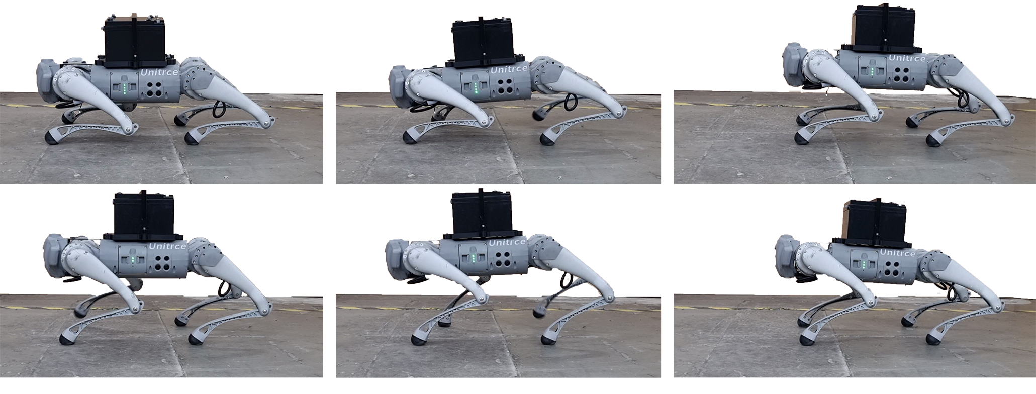
We experimentally validated our multi-contact inertial estimation and localization in trials with the Go1 robot. To showcase its capability in inertial estimation, we added an unknown payload of $7.2\text{\,}\mathrm{kg}$ to the robot’s torso, as depicted in Fig. 4. The observations recorded when the Go1’s predictive controller was unaware of the additional payload (Fig. 4-top).

Figure 4: Go1 performing four walking gaits while carrying an unknown payload. In the top snapshots, Go1 struggled to maintain its posture due to model mistmatch in the MPC. In the bottom snapshots, after correctly estimating the robot’s payload, Go1 confidently maintained its nominal posture.

We integrated a variety of observation sources with a step integration interval of $1\text{\,}\mathrm{ms}$. First, leveraging data from Go1’s encoders, we included joint positions $\mathbf{q}_{j}\in\mathbb{R}^{12}$ and numerically differentiated them to account for joint velocities $\mathbf{v}_{j}\in\mathbb{R}^{12}$. Second, we derived Go1’s torso rotation from the IMU’s sensor fusion algorithm. This was incorporated with the following observation model $\|\mathbf{\hat{\mathbf{R}}}_{b}\ominus\mathbf{R}_{b}\|^{2}_{\boldsymbol{\Sigma}_{\mathbf{R}}^{-1}}$. Here, $\mathbf{\hat{\mathbf{R}}}_{b}\ominus\mathbf{R}_{b}$ denotes the SO(3) inverse composition between the measured body orientation $\mathbf{\hat{\mathbf{R}}}_{b}$ and the estimated one $\mathbf{R}_{b}$ and $\boldsymbol{\Sigma}_{\mathbf{R}}\in S(3)$ represents the covariance estimated by the sensor fusion algorithm. Third, we pre-integrated the IMU’s linear acceleration to obtain the torso’s linear velocities. This observation also encompasses the IMU’s angular velocities, both of them are expressed in local coordinates for efficiency reasons. Lastly, we incorporated the torque commands $\mathbf{\hat{u}}\in\mathbb{R}^{12}$ applied by the state-feedback controller and measured contact sequences.

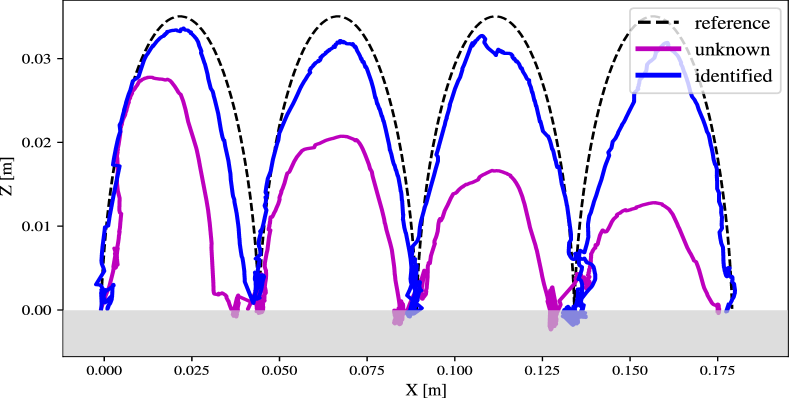
Figure 5: Foot-swing tracking of the Go1 robot when carrying an unknown payload. Our MPC encountered difficulties in tracking the reference swing-foot trajectory (dashed line) when the payload was unknonw (red line). Specifically, the Go1 robot failed to reach the desired step height, an error accumulated over time. In contrast, our MPC improved its foot-swing tracking performance when our estimator identified the payload (green line).

VI-C1 Estimating an unknown payload

The optimal estimator ran offline, estimating the inertial parameters after $27$ iterations. Within the estimation horizon of $14\text{\,}\mathrm{s}$, it accurately determined the total payload inertia, equivalent to a mass of $7.364\text{\,}\mathrm{kg}$. Subsequently, we updated the inertial parameters of Go1’s torso in its full-dynamics MPC. The impact of this update is vividly illustrated in Fig. 4-bottom. Concretely, it enabled the Go1 robot to maintain a stable posture during walking, emphasizing the significance of correcting model mismatches even for a fast MPC running at $50\text{\,}\mathrm{Hz}$.

The payload estimation significantly influences the tracking capabilities of the swing foot, as depicted in Fig. 5. A comparison between swing trajectories with and without inertial estimation reveals the crucial role it plays. In the absence of accurate inertial parameters, the MPC struggled to track reference swing trajectories, resulting in a progressively decaying motion (Fig. 4-top). Instead, when the inertia was estimated, the MPC adeptly tracked the swing trajectory.

VI-C2 Localization with hybrid dynamics

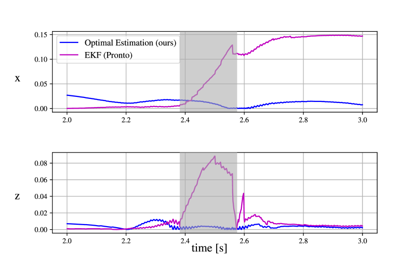
We compared our multi-contact localization approach against Pronto [35]–a widely adopted localization framework for legged robots based on extended Kalman filter (EKF) and leg kinematics. To assess the impact of incorporating hybrid dynamics, Pronto and the optimal estimator were configured to integrate proprioceptive information, namely IMU and encoders, exclusively, as done above. To provide a holistic evaluation, we employed Pronto to close the loop with our MPC. Fig. 6 shows localization errors for both estimators, measured through motion capture.

The inclusion of hybrid dynamics significantly improved localization accuracy, especially in the presence of a dynamic maneuver like a jump, leading to our optimal estimator outperforming Pronto’s estimation. This achievement is noteworthy because introducing the dynamics corrects almost all IMU drifts.

Figure 6: Go1’s localization errors when performing a jump. Our optimal estimator (blue lines) exhibits a smaller estimation error compared to Pronto.

VII Conclusion

We introduced (i) a multiple shooting optimal estimation algorithm tailored for multi-contact inertial estimation and localization and (ii) a novel smooth manifold with local submersion, named exponential eigenvalue, to ensure the full physical consistency of inertial parameters. Our exponential eigenvalue manifold was compared against the singularity-free log-Cholesky manifold, demonstrating improved convergence attributed to its reduced degree of nonlinearity. However, it presented singularities with symmetrical inertias. To address this, we proposed a nullspace approach, which handles these rank deficiencies. Additionally, our multiple-shooting rollout demonstrated superior numerical behavior compared to existing methods, resulting in better estimations. We demonstrated the effectiveness of our optimal estimation framework in complex scenarios such as humanoid brachiation and backflips. Practical benefits were further illustrated through experimental trials on the Go1 robot. Future work will involve an open-source C++ implementation and MHE development.