4University of Oxford 5Microsoft 6Nanyang Technological University
MVSplat: Efficient 3D Gaussian Splatting
from Sparse Multi-View Images
Abstract
We propose MVSplat, an efficient feed-forward 3D Gaussian Splatting model learned from sparse multi-view images. To accurately localize the Gaussian centers, we propose to build a cost volume representation via plane sweeping in the 3D space, where the cross-view feature similarities stored in the cost volume can provide valuable geometry cues to the estimation of depth. We learn the Gaussian primitives’ opacities, covariances, and spherical harmonics coefficients jointly with the Gaussian centers while only relying on photometric supervision. We demonstrate the importance of the cost volume representation in learning feed-forward Gaussian Splatting models via extensive experimental evaluations. On the large-scale RealEstate10K and ACID benchmarks, our model achieves state-of-the-art performance with the fastest feed-forward inference speed (22 fps). Compared to the latest state-of-the-art method pixelSplat, our model uses fewer parameters and infers more than faster while providing higher appearance and geometry quality as well as better cross-dataset generalization.
Keywords:
Feature Matching Cost Volume Gaussian Splatting![[Uncaptioned image]](/html/2403.14627/assets/x1.png)
1 Introduction
3D scene reconstruction and novel view synthesis from very sparse (i.e., as few as two) images pose a fundamental challenge in computer vision. While remarkable progress has been made using neural scene representations, e.g., Scene Representation Networks (SRN) [25], Neural Radiance Fields (NeRF) [16] and Light Filed Networks (LFN) [24], these methods are still not satisfactory for practical applications due to expensive per-scene optimization [18, 29, 32], high memory cost [2, 11, 33] and slow rendering speed [30, 38].
Recently, 3D Gaussian Splatting (3DGS) [12] has emerged as an efficient and expressive 3D representation thanks to its fast rendering speed and high quality. Using rasterization-based rendering, 3DGS inherently avoids the expensive volumetric sampling process of NeRF, leading to highly efficient and high-quality 3D reconstruction and novel view synthesis.
Subsequently, several feed-forward Gaussian Splatting methods have been proposed to explore 3D reconstruction from sparse view images, notably Splatter Image [27] and pixelSplat [1]. Splatter Image regresses pixel-aligned Gaussian parameters from a single view using a U-Net architecture, which achieves promising results for single object 3D reconstruction. However, 3D reconstruction from a single image is inherently ill-posed and ambiguous, which makes it particularly challenging to apply to more general and larger scene-level reconstruction, the key focus of our paper. For general scene reconstruction, pixelSplat [1] proposes to regress Gaussian parameters from two input views. Specifically, pixelSplat predicts a probabilistic depth distribution from features, and then depths are sampled from the learned distribution. Despite pixelSplat learns cross-view-aware features with an epipolar transformer, it is still challenging to predict a reliable probabilistic depth distribution solely from image features, making pixelSplat’s geometry reconstruction of comparably low quality and exhibit noisy artifacts (see Fig. 1 and Fig. 4). For improved geometry reconstruction results, slow depth finetuning with an additional depth regularization loss is required.
To accurately localize the 3D Gaussian centers, we propose to build a cost volume representation via plane sweeping [37, 35] in 3D space. Specifically, the cost volume stores cross-view feature similarities for all potential depth candidates, where the similarities can provide valuable geometry cues to the localization of 3D surfaces (e.g., high similarity more likely indicates a surface point). With our cost volume representation, the task is formulated as learning to perform feature matching to identify the Gaussian centers, unlike the data-driven 3D regression from image features in previous works [27, 1]. Such a formulation reduces the task’s learning difficulty, enabling our method to achieve state-of-the-art performance with lightweight model size and fast speed.
We obtain 3D Gaussian centers by unprojecting the multi-view-consistent depths estimated by our constructed multi-view cost volumes with a 2D network. Additionally, we also predict other Gaussian properties (covariance, opacity and spherical harmonics coefficients), in parallel with the depths. This enables the rendering of novel view images using the predicted 3D Gaussians with the differentiable splatting operation [12]. Our full model MVSplat is trained end-to-end purely with the photometric loss between rendered and ground truth images.
On the large-scale RealEstate10K [42] and ACID [14] benchmarks, our cost volume-based method MVSplat achieves state-of-the-art performance with the fastest feed-forward inference speed (22 fps). Compared to the state-of-the-art pixelSplat [1] (see Fig. 1), our model uses fewer parameters and infers more than faster while providing higher appearance and geometry quality as well as better cross-dataset generalization. Extensive ablation studies and analysis underscore the significance of our feature matching-based cost volume design in enabling highly efficient feed-forward 3D Gaussian Splatting models.
2 Related Work
Sparse View Scene Reconstruction and Synthesis. The original NeRF and 3DGS methods are both designed for very dense views (e.g., 100) as inputs, which can be tedious to capture for real-world applications. Recently, there have been growing interests [18, 29, 2, 3, 33, 1, 32] in scene reconstruction and synthesis from sparse input views (e.g., 2 or 3). Existing sparse view methods can be broadly classified into two categories: per-scene optimization and cross-scene feed-forward inference methods. Per-scene approaches mainly focus on designing effective regularization terms [18, 29, 39, 4, 32] to better constrain the optimization process. However, they are inherently slow at inference time due to the expensive per-scene gradient back-propagation process. In contrast, feed-forward models [38, 2, 3, 33, 1, 27] learn powerful priors from large-scale datasets, so that 3D reconstruction and view synthesis can be achieved via a single feed-forward inference by taking sparse views as inputs, which makes them significantly faster than per-scene optimization methods.
Feed-Forward NeRF. pixelNeRF [38] pioneered the paradigm of predicting pixel-aligned features from images for radiance field reconstruction. The performance of feed-forward NeRF models progressively improved with the use of feature matching information [2, 3], Transformers [21, 6, 17] and 3D volume representations [2, 33]. The state-of-the-art feed-forward NeRF model MuRF [33] is based on a target view frustum volume and a (2+1)D CNN for radiance field reconstruction, where the 3D volume and CNN need to be constructed and inferred for every target view. This makes MuRF expensive to train, with comparably slow rendering. Most importantly, all existing feed-forward NeRF models suffer from an expensive per-pixel volume sampling in the rendering process.
Feed-Forward 3DGS. 3D Gaussian Splatting avoids NeRF’s expensive volume sampling via a rasterization-based splatting approach, where novel views can be rendered very efficiently from a set of 3D Gaussian primitives. Very recently, a few feed-forward 3DGS models have been proposed to solve the sparse view to 3D task. Splatter Image [27] proposes to regress pixel-aligned Gaussian parameters from a single view with a U-Net. However, it mainly focuses on single object reconstruction, while we target a more general setting and larger scenes. pixelSplat [1] proposes to regress Gaussian parameters from two input views, where the epipolar geometry is leveraged to learn cross-view aware features. However, it estimates depth by sampling from a predicted distribution, which is ambiguous and can lead to poor geometry reconstruction. In contrast, we learn to predict depth directly from the feature matching information encoded within a cost volume, which makes it more geometry-aware and leads to a more lightweight model ( fewer parameters and more than faster) and significantly better geometries. Another related work GPS-Gaussian [41] proposes a feed-forward Gaussian model for the reconstruction of humans, instead of general scenes. It relies on two rectified stereo images to estimate the disparity, while our method works for general unrectified multi-view posed images. During training, GPS-Gaussian requires ground truth depth for supervision, while our model is trained from RGB images alone.
Multi-View Stereo. Multi-View Stereo (MVS) is a classic technique for reconstructing 3D scene structures from 2D images. Despite the conceptual similarity with the well-established MVS reconstruction pipeline [22, 37, 7], our approach possesses unique advantages. Unlike typical MVS methods involving separate depth estimation and point cloud fusion stages, we exploit the unique properties of the 3DGS representation to infer 3D structure in a single step, simply considering the union of the unprojected per-view depth predictions as the global 3D representation. Besides, existing MVS networks [37, 7, 5] are mostly trained with ground truth depth as supervision. In contrast, our model is fully differentiable and does not require ground truth geometry supervision for training, making it more scalable and suitable for in-the-wild scenarios.

3 Method
We begin with sparse-view images , () and their corresponding camera projection matrices , , calculated via intrinsic , rotation and translation matrices. Our goal is to learn a mapping from images to 3D Gaussian parameters:
| (1) |
where we parameterize as a feed-forward network and are the learnable parameters optimized from a large-scale training dataset. We predict the Gaussian parameters, including position , opacity , covariance and color (represented as spherical harmonics) in a pixel-aligned manner, and thus the total number of 3D Gaussians is for input images with shape .
To enable high-quality rendering and reconstruction, it is crucial to predict the position precisely since it defines the center of the 3D Gaussian [12]. In this paper, we present MVSplat, a Gaussian-based feed-forward model for novel view synthesis. Unlike pixelSplat [1] that predicts probabilistic depth, we develop an efficient and high-performance multi-view depth estimation model that enables unprojecting predicted depth maps as the Gaussian centers, in parallel with another branch for prediction of other Gaussian parameters (, and ). Our full model, illustrated in Fig. 2, is trained end-to-end using only a simple rendering loss for supervision. Next, we discuss key components.
3.1 Multi-View Depth Estimation
Our depth model is purely based on 2D convolutions and attentions, without any 3D convolutions used in many previous MVS [37, 7, 5] and feed-forward NeRF [2, 33] models. This makes our model highly efficient. Our depth model includes multi-view feature extraction, cost volume construction, cost volume refinement, depth estimation, and depth refinement, as introduced next.
Multi-view feature extraction. To construct the cost volumes, we first extract multi-view image features with a CNN and Transformer architecture [34, 35]. More specifically, a shallow ResNet-like CNN is first used to extract downsampled per-view image features, and then we use a multi-view Transformer with self- and cross-attention layers to exchange information between different views. For better efficiency, we use Swin Transformer’s local window attention [15] in our Transformer architecture. When more than two views are available, we perform cross-attention for each view with respect to all the other views, which has exactly the same learnable parameters as the 2-view scenario. After this operation, we obtain cross-view aware Transformer features (), where denotes the channel dimension.
Cost volume construction. An important component of our model is the cost volume, which models cross-view feature matching information with respect to different depth candidates via the plane-sweep stereo approach [37, 35]. Note that we construct cost volumes for input views to predict depth maps. Here, we take view ’s cost volume construction as an example. Given the near and far depth ranges, we first uniformly sample depth candidates in the inverse depth domain and then warp view ’s feature to view with the camera projection matrices , and each depth candidate , to obtain warped features
| (2) |
where denotes the warping operation [35]. We then compute the dot product [36, 35] between and to obtain the correlation
| (3) |
When there are more than two views as inputs, we similarly warp another view’s feature to view as in Eq. 2 and compute their correlations via Eq. 3. Finally, all the correlations are pixel-wise averaged, enabling the model to accept an arbitrary number of views as inputs.
Collecting all the correlations we obtain view ’s cost volume
| (4) |
Overall, we obtain cost volumes for input views.
Cost volume refinement. As the cost volume in Eq. 4 can be ambiguous for texture-less regions, we propose to further refine it with an additional lightweight 2D U-Net [20, 19]. The U-Net takes the concatenation of Transformer features and cost volume as inputs, and outputs a residual that is added to the initial cost volume . We obtain the refined cost volume as
| (5) |
To exchange information between cost volumes of different views, we inject three cross-view attention layers at the lowest resolution of the U-Net architecture. The cross-view attention layers are able to accept arbitrary number of views as input since it computes the cross-attention for each view with respect to all the other views, where such an operation does not depend on the number of views. The low-resolution cost volume is finally upsampled to full resolution with a CNN-based upsampler.
Depth estimation. We use the softmax operation to obtain per-view depth predictions. Specifically, we first normalize the refined cost volume in the depth dimension and then perform a weighted average of all depth candidates :
| (6) |
Depth refinement. To further improve the performance, we introduce an additional depth refinement step to enhance the quality of the above predicted depth. The refinement is performed with a very lightweight 2D U-Net, which takes multi-view images, features and current depth predictions as input, and outputs per-view residual depths. The residual depths are then added to the current depth predictions as the final depth outputs. Similar to the U-Net used in the above cost volume refinement, we also introduce cross-view attention layers in the lowest resolution to exchange information across views. More implementation details are presented in the supplementary material Appendix 0.C.
3.2 Gaussian Parameters Prediction
Gaussian centers . After obtaining the multi-view depth predictions, we directly unproject them to 3D point clouds using the camera parameters. We transform the per-view point cloud into an aligned world coordinate system and directly combine them as the centers of the 3D Gaussians.
Opacity . From the matching distribution obtained via the operation in Eq. 6, we can also obtain the matching confidence as the maximum value of the softmax output. Such matching confidence shares a similar physical meaning with the opacity (points with higher matching confidence are more likely to be on the surface), and thus we use two convolution layers to predict the opacity from the matching confidence input.
Covariance and color . We predict these parameters by two convolution layers that take as inputs the concatenated image features, refined cost volume and the original multi-view images. Similar to other 3DGS approaches [12, 1], the covariance matrix is composed of a scaling matrix and a rotation matrix represented via quaternions, and the color is calculated from the predicted spherical harmonic coefficients.
3.3 Training Loss
Our model predicts a set of 3D Gaussian parameters , which are then used for rendering images at novel viewpoints. Our full model is trained with ground truth target RGB images as supervision. The training loss is calculated as a linear combination of and LPIPS [40] losses, with loss weights of 1 and 0.05, respectively.
4 Experiments
4.1 Settings
Datasets. We assess our model on the large-scale RealEstate10K [42] and ACID [14] datasets. RealEstate10K contains real estate videos downloaded from YouTube, which are split into 67,477 training scenes and 7,289 testing scenes, while ACID contains nature scenes captured by aerial drone, split into 11,075 training scenes and 1,972 testing scenes. Both datasets provide estimated camera intrinsic and extrinsic parameters for each frame. Following pixelSpalt [1], we evaluate all methods on three target novel viewpoints for each test scene. Furthermore, to further evaluate the cross-dataset generalization ability, we also directly evaluate on the multi-view DTU [10] dataset, which contains object-centric scenes with camera poses. On DTU dataset, we report results on 16 validation scenes, with 4 novel views for each scene.
Metrics. For quantitative results, we report the standard image quality metrics, including pixel-level PSNR, patch-level SSIM [31], and feature-level LPIPS [40]. The inference time and model parameters are also reported to enable thorough comparisons of speed and accuracy trade-offs. For a fair comparison, all experiments are conducted on resolutions following existing models [1, 27].
Implementation details. Our MVSplat is implemented with PyTorch, along with an off-the-shelf 3DGS render implemented in CUDA. Our multi-view Transformer contains 6 stacked self- and cross-attention layers. We sample 128 depth candidates when constructing the cost volumes in all the experiments. All models are trained on a single A100 GPU for 300,000 iterations with the Adam [13] optimizer. More details are provided in the supplementary material Appendix 0.C. Code and models are available at https://github.com/donydchen/mvsplat.
4.2 Main Results
| Method | Time (s) | Param (M) | RealEstate10K [42] | ACID [14] | |||||
|---|---|---|---|---|---|---|---|---|---|
| PSNR | SSIM | LPIPS | PSNR | SSIM | LPIPS | ||||
| pixelNeRF [38] | 5.299 | 28.2 | 20.43 | 0.589 | 0.550 | 20.97 | 0.547 | 0.533 | |
| GPNR [26] | 13.340 | 9.6 | 24.11 | 0.793 | 0.255 | 25.28 | 0.764 | 0.332 | |
| AttnRend [6] | 1.325 | 125.1 | 24.78 | 0.820 | 0.213 | 26.88 | 0.799 | 0.218 | |
| MuRF [33] | 0.186 | 5.3 | 26.10 | 0.858 | 0.143 | 28.09 | 0.841 | 0.155 | |
| pixelSplat [1] | 0.104 | 125.4 | 25.89 | 0.858 | 0.142 | 28.14 | 0.839 | 0.150 | |
| MVSplat | 0.044 | 12.0 | 26.39 | 0.869 | 0.128 | 28.25 | 0.843 | 0.144 | |
Baselines. We compare MVSplat with several representative feed-forward methods that focus on scene-level novel view synthesis from sparse views, including i) Light Field Network-based GPNR [26] and AttnRend [6], ii) NeRF-based pixelNeRF [38] and MuRF [33], iii) the latest state-of-the-art 3DGS-based model pixelSplat [1]. We conduct thorough comparisons with the latter, being the most closely related to our method.
Assessing image quality. We report results on the RealEstate10K [42] and ACID [14] benchmarks in Tab. 1. Our MVSplat surpasses all previous state-of-the-art models in terms of all metrics on visual quality, with more obvious improvements in the LPIPS metric, which is better aligned with human perception. This includes pixelNeRF [38], GPNR [26], AttnRend [6] and pixelSplat [1], with results taken directly from the pixelSplat [1] paper, and the recent state-of-the-art NeRF-based method MuRF [33], for which we re-train and evaluate its performance using the officially released code.
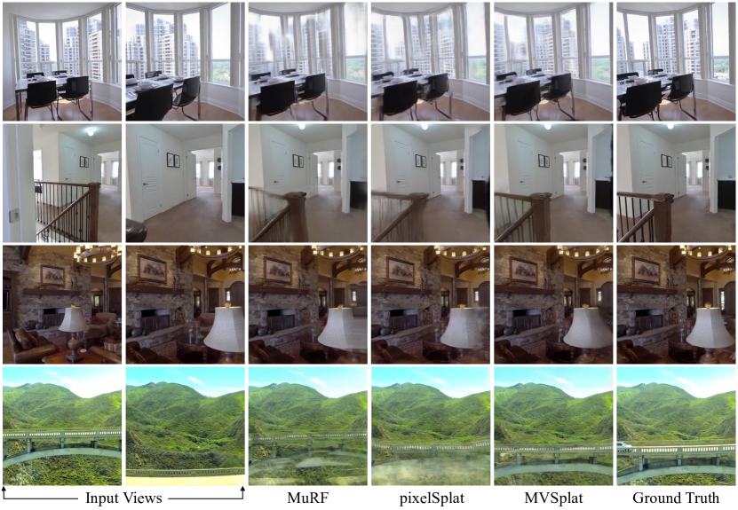
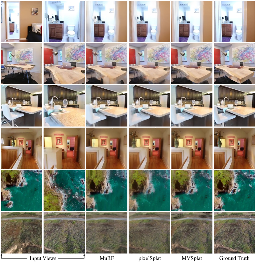
The qualitative comparisons of the top three best models are visualized in Fig. 3. MVSplat achieves the highest quality on novel view results even under challenging conditions, such as these regions with repeated patterns (“window frames” in 1st row), or these present in only one of the input views (“stair handrail” and “lampshade” in 2nd and 3rd rows), or when depicting large-scale outdoor objects captured from distant viewpoints (“bridge” in 4th row). The baseline methods exhibit obvious artifacts for these regions, while our MVSplat shows no such artifacts due to our cost volume-based geometry representation. More evidence and detailed analysis regarding how MVSplat effectively infers the geometry structures are presented in Sec. 4.3.
Assessing model efficiency. As reported in Tab. 1, apart from attaining superior image quality, our MVSplat also shows the fastest inference time among all the compared models, accompanied by a lightweight model size, demonstrating its efficiency and practical utility. It is noteworthy that the reported time encompasses both image encoding and rendering stages. For an in-depth time comparison with pixelSplat [1], our encoder runs at 0.043s, which is more than faster than pixelSplat (0.102s). Besides, pixelSplat predicts 3 Gaussians per-pixel, while our MVSplat predicts 1 single Gaussian, which also contributes to our faster rendering speed (0.0015s vs. 0.0025s) due to the threefold reduction in the number of Gaussians. More importantly, equipped with the cost volume-based encoder, our MVSplat enables fast feed-forward inference of 3D Gaussians with a much light-weight design, resulting in fewer parameters and more than faster speed compared to pixelSplat [1].
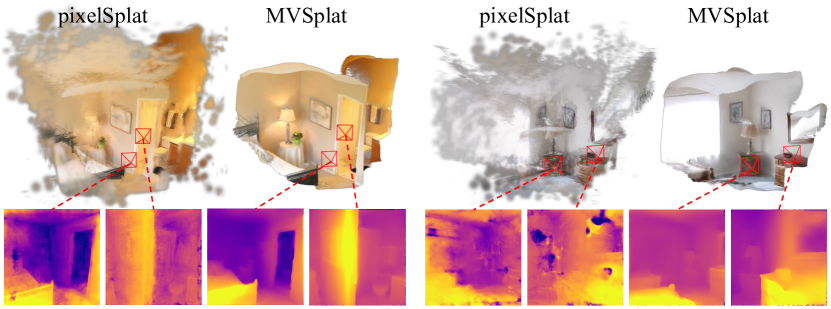
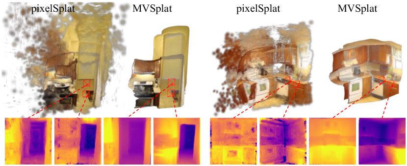
Assessing geometry reconstruction. Our MVSplat also produces significantly higher-quality 3D Gaussian primitives compared to the latest state-of-the-art pixelSplat [1], as demonstrated in Fig. 4. pixelSplat requires an extra 50,000 steps to fine-tune the Gaussians with an additional depth regularization to achieve reasonable geometry reconstruction results. Our MVSplat instead generates high-quality geometries by training solely with photometric supervision. Fig. 4 demonstrates the feed-forward geometry reconstruction results of our MVSplat, without any extra fine-tuning. Notably, although pixelSplat showcases reasonably rendered 2D images, its underlying 3D structure contains a large amount of floating Gaussians. In contrast, our MVSplat reconstructs much higher-quality 3D Gaussians, demonstrating the effectiveness of our cost volume representation in obtaining high-quality geometry structures. To facilitate a clearer understanding of the difference between the two methods, we invite the reader to view the corresponding “.ply” files of the exported 3D Gaussians in our project page.
| Training data | Method | ACID [14] | DTU [10] | ||||
|---|---|---|---|---|---|---|---|
| PSNR | SSIM | LPIPS | PSNR | SSIM | LPIPS | ||
| RealEstate10K [42] | pixelSplat [1] | 27.64 | 0.830 | 0.160 | 12.89 | 0.382 | 0.560 |
| MVSplat | 28.15 | 0.841 | 0.147 | 13.94 | 0.473 | 0.385 | |
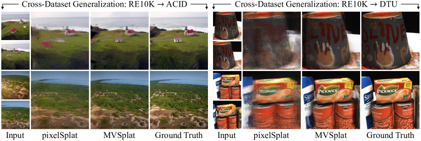
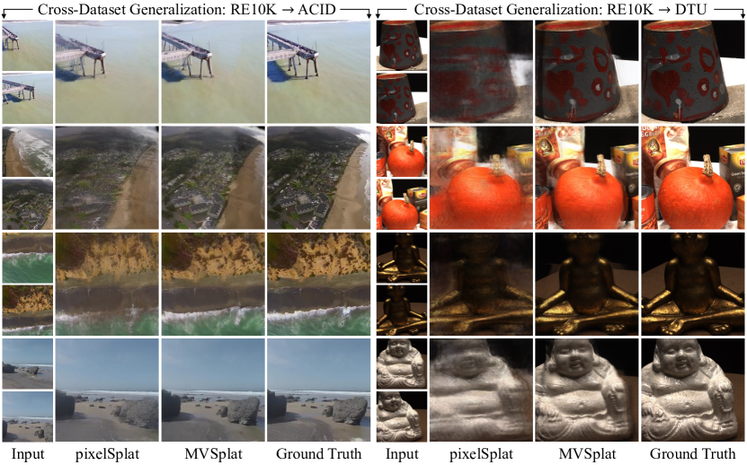
Assessing cross-dataset generalization. MVSplat is inherently superior in generalizing to out-of-distribution novel scenes, primarily due to the fact that the cost volume captures the relative similarity between features, which remains invariant compared to the absolute scale of features. To demonstrate this advantage, we conduct two cross-dataset evaluations. Specifically, we choose models trained solely on the RealEstate10K (indoor scenes), and directly test them on ACID (outdoor scenes) and DTU (object-centric scenes). As evident in Fig. 5, MVSplat renders competitive novel views, despite scenes of the targeted datasets contain significantly different camera distributions and image appearance from those of the source dataset. In contrast, views rendered by pixelSplat degrade dramatically; the main reason is likely that pixelSplat relies on purely feature aggregations that are tied to the absolute scale of feature values, hindering its performance when it receives different image features from other datasets. Quantitative results reported in Tab. 2 further uphold this observation. Note that the MVSplat significantly outperforms pixelSplat in terms of LPIPS, and the gain is larger when the domain gap between source and target datasets becomes larger. Surprisingly, our cross-dataset generalization results on ACID even slightly surpass the pixelSplat model that is specifically trained on ACID (see Tab. 1). We attribute such results to the larger scale of the RealEstate10K training set ( larger than ACID) and our superior generalization ability. This also suggests the potential of our method for training on more diverse and larger scale datasets in the future.
Assessing more-view quality. Our MVSplat is designed to be agnostic to the number of input views, so that it can benefit from more input views if they are available in the testing phase, regardless of how many input views are used in training. We verify this by testing on DTU with 3 context views, using the model trained on the 2-view RealEstate10K dataset. Our results are PSNR: 14.30, SSIM: 0.508, LPIPS: 0.371, and pixelSplat’s are PSNR: 12.52, SSIM: 0.367, LPIPS: 0.585. Compared to the 2-view results (Tab. 2), MVSplat achieves better performance with more input views. However, pixelSplat performs slightly worse when using more views, even though we have made our best effort to extend its released 2-views-only model to support more-view testing. This suggests that the feature distribution of more views might be different from the two views one used to train pixelSplat. This discrepancy is attributed to the reliance of pixelSplat on pure feature aggregation, which lacks robustness to changes in feature distribution. This limitation is analogous to the reason why pixelSplat performs inferior in cross-dataset generalization tests discussed earlier.
| Setup | PSNR | SSIM | LPIPS |
|---|---|---|---|
| base + refine | 26.39 | 0.869 | 0.128 |
| base | 26.12 | 0.864 | 0.133 |
| w/o cost volume | 22.83 | 0.753 | 0.197 |
| w/o cross-view attention | 25.19 | 0.852 | 0.152 |
| w/o U-Net | 25.45 | 0.847 | 0.150 |
4.3 Ablations
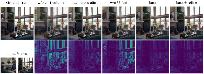
We conduct thorough ablations on RealEstate10K to analyze MVSplat. Results are shown in Tab. 3 and Fig. 6, and we discuss them in detail next. Our full model without “depth refinement” (Sec. 3.1) is regarded as the “base”.
Importance of cost volume. The cost volume serves as a cornerstone to the success of our MVSplat, which plays the most important role in our encoder to provide better geometry quality. To measure our cost volume scheme’s importance, we compare MVSplat to its variant (w/o cost volume) in Tab. 3. When removing it from the “base” model, the quantitative results drop significantly: it decreases the PSNR by more than 3dB, and increases LPIPS by 0.064 (nearly 50% relative degradation). This deterioration is more obviously evident in the rendered visual result in Fig. 6. The variant “w/o cost volume” exhibits a direct overlay of the two input views, indicating that the 3D Gaussian parameters extracted from the two input views fail to align within the same 3D space.
Ablations on cross-view attention. The cross-view matching is significant in learning multi-view geometry. The feature extraction backbone in our MVSplat is assembled with cross-view attention to enhance the feature expressiveness by fusing information between input views. We investigate it by removing the cross-view attention in our transformer. The quantitative results in Tab. 3 (“w/o cross-attn”) show a performance drop of 1dB PSNR, and the visual results in Fig. 6 (“w/o cross-attn”) showcase higher error intensity. This highlights the necessity for information flow between views. Besides, we also observe that this variant “w/o cross-attn” suffers from over-fitting (details shown in the supplementary material Fig. A), further confirming that this component is critical for model robustness. Due to the over-fitting issue, we report this variant specifically with its best performance instead of the final over-fitted one.
Ablations on the cost volume refinement U-Net. The initial cost volume might be less effective in challenging regions, thus we propose to use a U-Net for refinement. To investigate its importance, we performed a study (“w/o U-Net”) that removes the U-Net architecture. Fig. 6 reveals that, for the middle regions, the variant “w/o U-Net” render as well as the “base” mode, where content is present in both input views; but its left & right parts show obvious degraded quality in this variant compared with the “base” modes, for which content is only present in one of the inputs. This is because our cost volume cannot find any matches in these regions, leading to poorer geometry cues. In such a scenario, the U-Net refinement is important for mapping high-frequency details from input views to the Gaussian representation, resulting in an overall improvement of dB PSNR as reported in Tab. 3.
Ablations on depth refinement. Additional depth refinement helps improve the depth quality, essentially leading to better visual quality. As in Tab. 3, “base + refine” achieves the best outcome, hence it is used as our final model.
More ablations. We further demonstrate in the supplementary material Appendix 0.A that our cost volume based design can also greatly enhance pixelSplat [1]. Swin Transformer is more suitable for our MVSplat than Epipolar Transformer [9]. Our MVSplat can benefit from predicting more Gaussian primitives. And our MVSplat is superior to existing methods even when training from completely random initialization for the entire model.
5 Conclusion
We present MVSplat, an efficient feed-forward 3D Gaussian Splatting model that is trained using sparse multi-view images. The key to our success is that we construct a cost volume to exploit multi-view correspondence information for better geometry learning, differs from existing approaches that resort to data-driven design. With a well-customized encoder tailored for 3D Gaussians primitives prediction, our MVSplat sets new state-of-the-art in two large-scale scene-level reconstruction benchmarks. Compared to the latest state-of-the-art method pixelSplat, our MVSplat uses fewer parameters and infers more than faster while providing higher appearance and geometry quality as well as better cross-dataset generalization.
Limitations and Discussions. Our model might produce unreliable results for reflective surfaces like glasses and windows, which are currently open challenges for existing methods (detailed in Appendix 0.A). Besides, our model is currently trained on the RealEstate10K dataset, where its diversity is not sufficient enough to generalize robustly to in-the-wild real-world scenarios despite its large scale. It would be an interesting direction to explore our model’s scalability to larger and more diverse training datasets (e.g., by mixing several existing scene-level datasets) in the future.
References
- [1] Charatan, D., Li, S., Tagliasacchi, A., Sitzmann, V.: pixelsplat: 3d gaussian splats from image pairs for scalable generalizable 3d reconstruction. In: CVPR (2024)
- [2] Chen, A., Xu, Z., Zhao, F., Zhang, X., Xiang, F., Yu, J., Su, H.: Mvsnerf: Fast generalizable radiance field reconstruction from multi-view stereo. In: ICCV (2021)
- [3] Chen, Y., Xu, H., Wu, Q., Zheng, C., Cham, T.J., Cai, J.: Explicit correspondence matching for generalizable neural radiance fields. In: arXiv (2023)
- [4] Deng, K., Liu, A., Zhu, J.Y., Ramanan, D.: Depth-supervised nerf: Fewer views and faster training for free. In: CVPR (2022)
- [5] Ding, Y., Yuan, W., Zhu, Q., Zhang, H., Liu, X., Wang, Y., Liu, X.: Transmvsnet: Global context-aware multi-view stereo network with transformers. In: CVPR (2022)
- [6] Du, Y., Smith, C., Tewari, A., Sitzmann, V.: Learning to render novel views from wide-baseline stereo pairs. In: CVPR (2023)
- [7] Gu, X., Fan, Z., Zhu, S., Dai, Z., Tan, F., Tan, P.: Cascade cost volume for high-resolution multi-view stereo and stereo matching. In: CVPR (2020)
- [8] He, K., Zhang, X., Ren, S., Sun, J.: Deep residual learning for image recognition. In: CVPR (2016)
- [9] He, Y., Yan, R., Fragkiadaki, K., Yu, S.I.: Epipolar transformers. In: CVPR (2020)
- [10] Jensen, R., Dahl, A., Vogiatzis, G., Tola, E., Aanæs, H.: Large scale multi-view stereopsis evaluation. In: CVPR (2014)
- [11] Johari, M.M., Lepoittevin, Y., Fleuret, F.: Geonerf: Generalizing nerf with geometry priors. In: CVPR (2022)
- [12] Kerbl, B., Kopanas, G., Leimkühler, T., Drettakis, G.: 3d gaussian splatting for real-time radiance field rendering. TOG 42(4) (2023)
- [13] Kingma, D.P., Ba, J.: Adam: A method for stochastic optimization. In: ICLR (2015)
- [14] Liu, A., Tucker, R., Jampani, V., Makadia, A., Snavely, N., Kanazawa, A.: Infinite nature: Perpetual view generation of natural scenes from a single image. In: ICCV (2021)
- [15] Liu, Z., Lin, Y., Cao, Y., Hu, H., Wei, Y., Zhang, Z., Lin, S., Guo, B.: Swin transformer: Hierarchical vision transformer using shifted windows. In: ICCV (2021)
- [16] Mildenhall, B., Srinivasan, P.P., Tancik, M., Barron, J.T., Ramamoorthi, R., Ng, R.: Nerf: Representing scenes as neural radiance fields for view synthesis. In: ECCV (2020)
- [17] Miyato, T., Jaeger, B., Welling, M., Geiger, A.: Gta: A geometry-aware attention mechanism for multi-view transformers. In: ICLR (2024)
- [18] Niemeyer, M., Barron, J.T., Mildenhall, B., Sajjadi, M.S., Geiger, A., Radwan, N.: Regnerf: Regularizing neural radiance fields for view synthesis from sparse inputs. In: CVPR (2022)
- [19] Rombach, R., Blattmann, A., Lorenz, D., Esser, P., Ommer, B.: High-resolution image synthesis with latent diffusion models. In: CVPR (2022)
- [20] Ronneberger, O., Fischer, P., Brox, T.: U-net: Convolutional networks for biomedical image segmentation. In: MICCAI (2015)
- [21] Sajjadi, M.S., Meyer, H., Pot, E., Bergmann, U., Greff, K., Radwan, N., Vora, S., Lučić, M., Duckworth, D., Dosovitskiy, A., et al.: Scene representation transformer: Geometry-free novel view synthesis through set-latent scene representations. In: CVPR (2022)
- [22] Schönberger, J.L., Zheng, E., Frahm, J.M., Pollefeys, M.: Pixelwise view selection for unstructured multi-view stereo. In: ECCV (2016)
- [23] Shi, Y., Wang, P., Ye, J., Long, M., Li, K., Yang, X.: Mvdream: Multi-view diffusion for 3d generation. ICLR (2024)
- [24] Sitzmann, V., Rezchikov, S., Freeman, B., Tenenbaum, J., Durand, F.: Light field networks: Neural scene representations with single-evaluation rendering. NeurIPS (2021)
- [25] Sitzmann, V., Zollhöfer, M., Wetzstein, G.: Scene representation networks: Continuous 3d-structure-aware neural scene representations. NeurIPS (2019)
- [26] Suhail, M., Esteves, C., Sigal, L., Makadia, A.: Generalizable patch-based neural rendering. In: ECCV (2022)
- [27] Szymanowicz, S., Rupprecht, C., Vedaldi, A.: Splatter image: Ultra-fast single-view 3d reconstruction. In: CVPR (2024)
- [28] Tang, J., Chen, Z., Chen, X., Wang, T., Zeng, G., Liu, Z.: Lgm: Large multi-view gaussian model for high-resolution 3d content creation. arXiv (2024)
- [29] Truong, P., Rakotosaona, M.J., Manhardt, F., Tombari, F.: Sparf: Neural radiance fields from sparse and noisy poses. In: CVPR (2023)
- [30] Wang, Q., Wang, Z., Genova, K., Srinivasan, P.P., Zhou, H., Barron, J.T., Martin-Brualla, R., Snavely, N., Funkhouser, T.: Ibrnet: Learning multi-view image-based rendering. In: CVPR (2021)
- [31] Wang, Z., Bovik, A.C., Sheikh, H.R., Simoncelli, E.P.: Image quality assessment: from error visibility to structural similarity. TIP 13(4) (2004)
- [32] Wu, R., Mildenhall, B., Henzler, P., Park, K., Gao, R., Watson, D., Srinivasan, P.P., Verbin, D., Barron, J.T., Poole, B., et al.: Reconfusion: 3d reconstruction with diffusion priors. arXiv (2023)
- [33] Xu, H., Chen, A., Chen, Y., Sakaridis, C., Zhang, Y., Pollefeys, M., Geiger, A., Yu, F.: Murf: Multi-baseline radiance fields. In: CVPR (2024)
- [34] Xu, H., Zhang, J., Cai, J., Rezatofighi, H., Tao, D.: Gmflow: Learning optical flow via global matching. In: CVPR (2022)
- [35] Xu, H., Zhang, J., Cai, J., Rezatofighi, H., Yu, F., Tao, D., Geiger, A.: Unifying flow, stereo and depth estimation. PAMI (2023)
- [36] Xu, H., Zhang, J.: Aanet: Adaptive aggregation network for efficient stereo matching. In: CVPR (2020)
- [37] Yao, Y., Luo, Z., Li, S., Fang, T., Quan, L.: Mvsnet: Depth inference for unstructured multi-view stereo. In: ECCV (2018)
- [38] Yu, A., Ye, V., Tancik, M., Kanazawa, A.: pixelnerf: Neural radiance fields from one or few images. In: CVPR (2021)
- [39] Yu, Z., Peng, S., Niemeyer, M., Sattler, T., Geiger, A.: Monosdf: Exploring monocular geometric cues for neural implicit surface reconstruction. NeurIPS (2022)
- [40] Zhang, R., Isola, P., Efros, A.A., Shechtman, E., Wang, O.: The unreasonable effectiveness of deep features as a perceptual metric. In: CVPR (2018)
- [41] Zheng, S., Zhou, B., Shao, R., Liu, B., Zhang, S., Nie, L., Liu, Y.: Gps-gaussian: Generalizable pixel-wise 3d gaussian splatting for real-time human novel view synthesis. In: CVPR (2024)
- [42] Zhou, T., Tucker, R., Flynn, J., Fyffe, G., Snavely, N.: Stereo magnification: learning view synthesis using multiplane images. TOG p. 65 (2018)
Appendix 0.A More Experimental Analysis
All experiments in this section follow the same settings as in Sec. 4.3 unless otherwise specified, which are trained on RealEstate10K [42] and reported by averaging over the full test set.
Using cost volume in pixelSplat. In the main paper, we have demonstrated the importance of our cost volume design for learning feed-forward Gaussian models. We note that such concept is general and is not specifically designed for a specific architecture. To verify this, we replace pixelSplat’s probability density-based depth prediction module with our cost volume-based approach while keeping other components intact. The results shown in Tab. A again demonstrate the importance of the cost volume by significantly outperforming the original pixelSplat, indicating the general applicability of our proposed method.
| Setup | PSNR | SSIM | LPIPS |
|---|---|---|---|
| pixelSplat (w/ probability density depth) [1] | 25.89 | 0.858 | 0.142 |
| pixelSplat (w/ our MVSplat cost volume depth) | 26.63 | 0.875 | 0.122 |
| Setup | Time (s) | PSNR | SSIM | LPIPS |
|---|---|---|---|---|
| MVSplat (w/ Epipolar Transformer [1]) | 0.055 | 26.09 | 0.865 | 0.133 |
| MVSplat (w/ Swin Transformer) | 0.038 | 26.12 | 0.864 | 0.133 |
Ablations on the backbone Transformer. Differing from pixelSplat [1] and GPNR [26] that are based on the Epipolar Transformer, we adopt Swin Transformer [15] in our backbone (i.e., Multi-view feature extraction as in Sec. 3.1). To compare the Transformer architectures, we conduct ablation experiment by replacing our Swin Transformer with the Epipolar Transformer in Tab. B. Since the Swin Transformer does not need to sample points on the epipolar line, where the sampling process is computationally expensive, our model is more efficient than the Epipolar Transformer counterpart. Besides, there is no clear difference observed in their rendering qualities, demonstrating the superiority of our Swin Transformer-based design.
| Setup | Render Time (s) | PSNR | SSIM | LPIPS |
|---|---|---|---|---|
| MVSplat (1 Gaussian per pixel) | 0.0015 | 26.39 | 0.869 | 0.128 |
| MVSplat (3 Gaussians per pixel) | 0.0023 | 26.54 | 0.872 | 0.127 |
Ablations on the Gaussian numbers per pixel. Unlike pixelSplat that predicts three Gaussians per image pixel, our MVSplat by default only predicts one per pixel. However, MVSplat can also benefit from increasing the number of Gaussians. As reported in Tab. C, our default model can be further boosted by predicting more Gaussians, but it also impacts the rendering speed. We choose to predict one Gaussian per pixel to balance performance and rendering speed.
| Method | PSNR | SSIM | LPIPS |
|---|---|---|---|
| pixelSplat w/ DINO init (300K) [1] | 25.89 | 0.858 | 0.142 |
| MVSplat w/ UniMatch init (300K) | 26.39 | 0.869 | 0.128 |
| MVSplat w/ random init (300K) | 26.01 | 0.863 | 0.133 |
| MVSplat w/ random init (450K) | 26.29 | 0.868 | 0.128 |
Ablations on backbone initialization. In our implementations, we initialize our backbone (i.e., Multi-view feature extraction as in Sec. 3.1) with the publicly available UniMatch [35] pretrained weight111https://github.com/autonomousvision/unimatch, where its training data has no overlap with any datasets used in our experiments. However, our model can also be trained with random initialization (“w/ random init”) and still outperforms previous state-of-the-art method pixelSplat [1], whose backbone is initialized with the weights pretrained on ImageNet with a DINO objective. To compensate for the lack of a proper initialization, our random initialized model needs more training iterations (450K) to reach the performance of the UniMatch initialized model. The results further demonstrate our model’s high efficiency and effectiveness, where strong performance can still be obtained without relying on pretraining on large-scale datasets.
Validation curves of the ablations. To better perceive the performance difference of different ablations, we provide the validation curves throughout the whole training phase in Fig. A). The cost volume plays a fundamental role in our full model, and interestingly, the model without cross-view attention suffers from overfitting after certain training iterations.


Limitation. Our MVSplat might be less effective on non-Lambertain and reflective surfaces, as shown in Fig. B. Integrating the rendering with additional BRDF properties and training the model with more diverse datasets might be helpful for addressing this issue in the future.
Potential negative societal impacts. Our model may produce unreliable outcomes, particularly when applied to complex real-world scenes. Therefore, it is imperative to exercise caution when implementing our model in safety-critical situations, e.g., when augmenting data to train models for autonomous vehicles with synthetic data rendered from our model.
Appendix 0.B More Visual Comparisons
In this section, we provide more qualitative comparisons of our MVSplat with state-of-the-art methods on the RealEstate10K and ACID in Fig. C. We also provide more comparisons with our main comparison model pixelSplat [1] regarding geometry reconstruction (see Fig. D) and cross-dataset generalizations (see Fig. E). Besides, readers are referred to the project page for the rendered videos and 3D Gaussians models (provided in “.ply” format).
Appendix 0.C More Implementation Details
Network architectures. Our shallow ResNet-like CNN is composed of 6 residual blocks [8], In the last 4 blocks, the feature is down-sampled to half after every 2 consecutive blocks by setting the convolution stride to 2, resulting in overall down sampling. The following Transformer consists of 6 stacked Transformer blocks, each of which contains one self-attention layer followed by one cross-attention layer. Swin Transformer’s [15] local window attention is used and the features are split into in all our experiments. For the cost volume refinement, we adopt the 2D U-Net implementations from [19]. We keep the channel dimension unchanged throughout the U-Net as 128, and apply 2 times of down-sampling, with an additional self-attention layer at the down-sampled level. Inspired by existing multi-view based models [23, 28], we also flatten the features before applying self-attention, allowing information to propagate among different cost volumes. The following depth refinement U-Net also shares a similar configuration, except that we apply 4 times of down-sampling and add attentions at the down-sampled level.
More training details. As aforementioned, we initialize the backbone of MVSplat in all experiments with the UniMatch [35] pretrained weight. Our default model is trained on a single A100 GPU. The batch size is set to 14, where each batch contains one training scene, including two input views and four target views. Similar to pixelSplat [1], the frame distance between two input views is gradually increased as the training progressed. For both RealEstate10K and ACID, we empirically set the near and far depth plane to 1 and 100, respectively, while for DTU, we set them to 2.125 and 4.525 as provided by the dataset.