(eccv) Package eccv Warning: Package ‘hyperref’ is loaded with option ‘pagebackref’, which is *not* recommended for camera-ready version

11institutetext:

Simplified Diffusion Schrödinger Bridge

Zhicong Tang 1*1*    Tiankai Hang 2*2*   
Shuyang Gu
3†3†
   Dong Chen 33    Baining Guo

1Tsinghua University 2Southeast University 3Microsoft Research Asia

tzc21@mails.tsinghua.edu.cn, tkhang@seu.edu.cn, {shuyanggu,doch,bainguo}@microsoft.com
33
Abstract

This paper introduces a novel theoretical simplification of the Diffusion Schrödinger Bridge (DSB) that facilitates its unification with Score-based Generative Models (SGMs), addressing the limitations of DSB in complex data generation and enabling faster convergence and enhanced performance. By employing SGMs as an initial solution for DSB, our approach capitalizes on the strengths of both frameworks, ensuring a more efficient training process and improving the performance of SGM. We also propose a reparameterization technique that, despite theoretical approximations, practically improves the network’s fitting capabilities. Our extensive experimental evaluations confirm the effectiveness of the simplified DSB, demonstrating its significant improvements. We believe the contributions of this work pave the way for advanced generative modeling. The code is available at https://github.com/checkcrab/SDSB.

Keywords:
Schrödinger Bridge Score-based Generative Models
00footnotetext: *Equal contribution.  \daggerCorresponding author.

1 Introduction

Score-based Generative Models (SGMs) [48, 24, 49] have recently achieved remarkable success, as highlighted in recent literature [14, 38, 39, 40, 20]. Despite their advancements, SGMs necessitate a carefully crafted schedule for adding noise, tailored to diverse tasks [27, 30, 19, 8]. Without this customization, training SGMs to handle complex data types, including video [5, 23, 1] and 3D contents [26, 50, 36], may present significant difficulties. Besides, SGMs are limited to modeling the target data distribution based on a predefined known distribution, e.g. Gaussian [49, 24], which narrows their applicability in certain scenarios, such as conditional generation tasks like unpaired domain transfer [53].

The Schrödinger Bridge (SB) problem [44, 17, 10] is considered a more generalized framework that construct a transition between two arbitrary distributions. Numerous approximations of SB have been proposed [45, 4, 9, 15, 6, 37], and one theoretical solution is the Iterative Proportional Fitting (IPF) [18, 28, 42]. Nevertheless, practical application remains challenging because it involves optimizing joint distributions, which can be highly complex. A recent work, Diffusion Schrödinger Bridge (DSB) [45], simplifies this by approximating the joint distribution optimization as a conditional distribution optimization problem. It employs two neural networks to enable the transition from one distribution to another by iteratively training them.

While DSB possesses theoretical superiority compared to SGMs, its practical implementation is hindered by a slow convergence rate and potential issues with network fitting capabilities [45]. Moreover, distinct training methodologies between DSB and SGM currently prevent the former from leveraging the rapid advancements being made in the field of SGM.

In this paper, we bridge the gap between the DSB and SGM by formulating a simplified optimization objective for DSB. Through this unification, SGM can be served as an initial solution for DSB, enabling enhanced outcomes with further iterations according to DSB [45]. Our theoretical analysis reveals that this initialization strategy is pivotal for the training of DSB, addressing the issue of slow convergence and yielding improved performance. Simultaneously, from the perspective of SGM, a pre-trained model can experience consistent enhancement through supplementary training using the DSB approach.

Furthermore, a key to the success of SGM [14, 40, 38] and other generative models, e.g. Flow Matching (FM) [31], Conditional Flow Matching (CFM) [51] and Rectified Flow [33], lies in their use of reparameterization [43, 24] to create a consistent output space across different timesteps, which maximizes the shared network’s fitting capabilities. Drawing inspiration from them, we propose a reparameterization trick to standardize the output space for the DSB. Despite the reliance on a considerable number of theoretical approximations, we were pleasantly surprised to discover that this also unlocked the network’s potential, subsequently speeding up convergence and leading to enhanced results.

We conduct comprehensive experiments to confirm the effectiveness of our proposed simplification and to showcase the significant enhancements it brings to DSB. Our contributions are summarized as follows:

  • We introduce a theoretical simplification of DSB, proving its equivalence to the original formulation.

  • By employing the simplified version, we successfully integrate SGM with DSB. Using SGM as the initialization for DSB significantly accelerates its convergence.

  • We devise a reparameterization technique that, despite some theoretical approximations, practically enhances the network’s fitting capabilities.

  • Through extensive experimentation, we examine practical training for DSB and validate the effectiveness of our proposed simplification.

2 Preliminary

In this section, we initiate by recalling some essential preliminaries of SGM in Section 2.1. Then, we introduce the SB problem and DSB, an approximate solution of it, in Section 2.2. Finally, in Section 2.3, we summarized prevalent dynamic generative models and unified them into the SDE form of SB.

Notation Consider a data distribution pdatasubscript𝑝datap_{\textup{data}} and a prior distribution ppriorsubscript𝑝priorp_{\textup{prior}}, each defined over the dsuperscript𝑑\mathbb{R}^{d} with positive density. We denote the transformation from pdatasubscript𝑝datap_{\textup{data}} to ppriorsubscript𝑝priorp_{\textup{prior}} as the forward process, whereas the reverse transformation as the backward process. The symbols k{0,,N}𝑘0𝑁k\in\{0,\dots,N\} and t[0,T]𝑡0𝑇t\in[0,T] represent discrete and continuous time horizons, respectively. In discrete-time scenarios, 𝒫l=𝒫((d)l)subscript𝒫𝑙𝒫superscriptsuperscript𝑑𝑙\mathscr{P}_{l}=\mathscr{P}\left((\mathbb{R}^{d})^{l}\right) signifies the probability of a l𝑙l-state joint distribution for any l𝑙l\in\mathbb{N}. In continuous-time scenarios, we use 𝒫(𝒞)𝒫𝒞\mathscr{P}(\mathcal{C}) where 𝒞=C([0,T],d)𝒞C0𝑇superscript𝑑\mathcal{C}=\textup{C}\left([0,T],\mathbb{R}^{d}\right). H(p)=p(x)logp(x)dxH𝑝𝑝𝑥𝑝𝑥differential-d𝑥\textup{H}(p)=-\int p(x)\log p(x)\mathrm{d}x denotes the entropy of p𝑝p. The Kullback-Leibler divergence between distributions p𝑝p and q𝑞q is defined by KL(p|q)=p(x)logp(x)q(x)dxKLconditional𝑝𝑞𝑝𝑥𝑝𝑥𝑞𝑥d𝑥\textup{KL}(p|q)=\int p(x)\log\frac{p(x)}{q(x)}\mathrm{d}x, and Jeffrey’s divergence is denoted as J(p|q)=12(KL(p|q)+KL(q|p))Jconditional𝑝𝑞12KLconditional𝑝𝑞KLconditional𝑞𝑝\textup{J}(p|q)=\frac{1}{2}\left(\textup{KL}(p|q)+\textup{KL}(q|p)\right).

2.1 Score-based Generative Models

Score-based Generative Models (SGMs) [48, 24, 47, 46] connect two distributions through a dual process: a forward process that transitions the data distribution, pdatasubscript𝑝datap_{\text{data}}, toward a prior distribution, ppriorsubscript𝑝priorp_{\text{prior}}, and a reverse process, typically guided by neural networks, that converts the prior back to the data distribution. These two processes can be modeled as Markov chains. Given an initial data distribution pdatasubscript𝑝datap_{\textup{data}} and a target prior distribution ppriorsubscript𝑝priorp_{\textup{prior}}, the forward process pk+1|k(xk+1|xk)subscript𝑝𝑘conditional1𝑘conditionalsubscript𝑥𝑘1subscript𝑥𝑘p_{k+1|k}(x_{k+1}|x_{k}) is designed to transition from p0=pdatasubscript𝑝0subscript𝑝datap_{0}=p_{\textup{data}} step-by-step towards a close approximation of ppriorsubscript𝑝priorp_{\textup{prior}}. This process generates a sequence x0:Nsubscript𝑥:0𝑁x_{0:N} from the (N+1)𝑁1(N+1) intermediate steps. This trajectory’s joint probability density is then formally defined as:

p(x0:N)=p0(x0)k=0N1pk+1|k(xk+1|xk).𝑝subscript𝑥:0𝑁subscript𝑝0subscript𝑥0superscriptsubscriptproduct𝑘0𝑁1subscript𝑝𝑘conditional1𝑘conditionalsubscript𝑥𝑘1subscript𝑥𝑘p(x_{0:N})=p_{0}(x_{0})\prod_{k=0}^{N-1}p_{k+1|k}(x_{k+1}|x_{k}). (1)

Through the backward process, the joint density can also be reformulated as a time-reversed distribution:

p(x0:N)=pN(xN)k=0N1pk|k+1(xk|xk+1)𝑝subscript𝑥:0𝑁subscript𝑝𝑁subscript𝑥𝑁superscriptsubscriptproduct𝑘0𝑁1subscript𝑝conditional𝑘𝑘1conditionalsubscript𝑥𝑘subscript𝑥𝑘1\displaystyle p(x_{0:N})=p_{N}(x_{N})\prod_{k=0}^{N-1}p_{k|k+1}(x_{k}|x_{k+1}) (2)
where pk|k+1(xk|xk+1)=pk+1|k(xk+1|xk)pk(xk)pk+1(xk+1),subscript𝑝conditional𝑘𝑘1conditionalsubscript𝑥𝑘subscript𝑥𝑘1subscript𝑝𝑘conditional1𝑘conditionalsubscript𝑥𝑘1subscript𝑥𝑘subscript𝑝𝑘subscript𝑥𝑘subscript𝑝𝑘1subscript𝑥𝑘1\displaystyle p_{k|k+1}(x_{k}|x_{k+1})=\frac{p_{k+1|k}(x_{k+1}|x_{k})p_{k}(x_{k})}{p_{k+1}(x_{k+1})},

However, directly computing pk|k+1(xk|xk+1)subscript𝑝conditional𝑘𝑘1conditionalsubscript𝑥𝑘subscript𝑥𝑘1p_{k|k+1}(x_{k}|x_{k+1}) is typically challenging. SGM utilizes a simplified approach that regard the forward process as a gradual adding of Gaussian noise:

pk+1|k(xk+1|xk)=𝒩(xk+1;xk+γk+1fk(xk),2γk+1𝐈).subscript𝑝𝑘conditional1𝑘conditionalsubscript𝑥𝑘1subscript𝑥𝑘𝒩subscript𝑥𝑘1subscript𝑥𝑘subscript𝛾𝑘1subscript𝑓𝑘subscript𝑥𝑘2subscript𝛾𝑘1𝐈p_{k+1|k}(x_{k+1}|x_{k})=\mathcal{N}(x_{k+1};x_{k}+\gamma_{k+1}f_{k}(x_{k}),2\gamma_{k+1}\mathbf{I}). (3)

It follows that for a sufficiently extensive N𝑁N, the distribution pNsubscript𝑝𝑁p_{N} will converge to Gaussian distribution, which we set as ppriorsubscript𝑝priorp_{\textup{prior}}. Moreover, the temporal inversion in Equation 2 can be analytically approximated [25, 52, 2] as

pk|k+1(xk|xk+1)subscript𝑝conditional𝑘𝑘1conditionalsubscript𝑥𝑘subscript𝑥𝑘1\displaystyle p_{k|k+1}(x_{k}|x_{k+1}) =pk+1|k(xk+1|xk)exp(logpk(xk)logpk+1(xk+1))absentsubscript𝑝𝑘conditional1𝑘conditionalsubscript𝑥𝑘1subscript𝑥𝑘subscript𝑝𝑘subscript𝑥𝑘subscript𝑝𝑘1subscript𝑥𝑘1\displaystyle=p_{k+1|k}(x_{k+1}|x_{k})\exp\left(\log p_{k}(x_{k})-\log p_{k+1}(x_{k+1})\right) (4)
𝒩(xk;xk+1γk+1fk+1(xk+1)+2γk+1logpk+1(xk+1),2γk+1𝐈)absent𝒩subscript𝑥𝑘subscript𝑥𝑘1subscript𝛾𝑘1subscript𝑓𝑘1subscript𝑥𝑘12subscript𝛾𝑘1subscript𝑝𝑘1subscript𝑥𝑘12subscript𝛾𝑘1𝐈\displaystyle\approx\mathcal{N}(x_{k};x_{k+1}-\gamma_{k+1}f_{k+1}(x_{k+1})+2\gamma_{k+1}\nabla\log p_{k+1}(x_{k+1}),2\gamma_{k+1}\mathbf{I})

under the assumption that pkpk+1subscript𝑝𝑘subscript𝑝𝑘1p_{k}\approx p_{k+1} and fk(xk)fk+1(xk+1)subscript𝑓𝑘subscript𝑥𝑘subscript𝑓𝑘1subscript𝑥𝑘1f_{k}(x_{k})\approx f_{k+1}(x_{k+1}). Subsequently, SGM employs neural networks sθ(xk+1,k+1)subscript𝑠𝜃subscript𝑥𝑘1𝑘1s_{\theta}(x_{k+1},k+1) to approximate the score term logpk+1(xk+1)subscript𝑝𝑘1subscript𝑥𝑘1\nabla\log p_{k+1}(x_{k+1}), thus the reverse process can be effectively modeled. By sampling xNppriorsimilar-tosubscript𝑥𝑁subscript𝑝priorx_{N}\sim p_{\textup{prior}}, followed by iteratively applying ancestral sampling via xkpk|k+1(xk|xk+1)similar-tosubscript𝑥𝑘subscript𝑝conditional𝑘𝑘1conditionalsubscript𝑥𝑘subscript𝑥𝑘1x_{k}\sim p_{k|k+1}(x_{k}|x_{k+1}), culminating in the estimation of x0pdatasimilar-tosubscript𝑥0subscript𝑝datax_{0}\sim p_{\textup{data}}.

The diffusion and denoising processes can also be formulated as continuous-time Markov chains. The forward process can be represented as a continuous-time Stochastic Differential Equation (SDE) [49]:

d𝐗t=ft(𝐗t)dt+2d𝐁t,dsubscript𝐗𝑡subscript𝑓𝑡subscript𝐗𝑡d𝑡2dsubscript𝐁𝑡\mathrm{d}\mathbf{X}_{t}=f_{t}(\mathbf{X}_{t})\mathrm{d}t+\sqrt{2}\mathrm{d}\mathbf{B}_{t}, (5)

where f:dd:𝑓superscript𝑑superscript𝑑f:\mathbb{R}^{d}\to\mathbb{R}^{d} is the drift term and (𝐁t)t[0,T]subscriptsubscript𝐁𝑡𝑡0𝑇(\mathbf{B}_{t})_{t\in[0,T]} denotes the Brownian motion, we called it the diffusion term. We note that the Markov chain with transition kernel (3) can be viewed as the Euler-Maruyama discretization of this SDE. The backward process, on the other hand, is conceptualized by solving the time-reversed SDE [22, 16, 7] which corresponds to (4):

d𝐘t=(ft(𝐘t)+2logpTt(𝐘t))dt+2d𝐁t.dsubscript𝐘𝑡subscript𝑓𝑡subscript𝐘𝑡2subscript𝑝𝑇𝑡subscript𝐘𝑡d𝑡2dsubscript𝐁𝑡\mathrm{d}\mathbf{Y}_{t}=\left(-f_{t}(\mathbf{Y}_{t})+2\nabla\log p_{T-t}(\mathbf{Y}_{t})\right)\mathrm{d}t+\sqrt{2}\mathrm{d}\mathbf{B}_{t}. (6)

2.2 Schrödinger Bridge and Diffusion Schrödinger Bridge

Consider a reference density pref𝒫N+1subscript𝑝refsubscript𝒫𝑁1p_{\textup{ref}}\in\mathscr{P}_{N+1} given by Equation 1, the Schrödinger Bridge (SB) problem aims to find π𝒫N+1superscript𝜋subscript𝒫𝑁1\pi^{*}\in\mathscr{P}_{N+1} which satisfies

π=argmin{KL(π|pref):π𝒫N+1,π0=pdata,πN=pprior}.superscript𝜋:KLconditional𝜋subscript𝑝refformulae-sequence𝜋subscript𝒫𝑁1formulae-sequencesubscript𝜋0subscript𝑝datasubscript𝜋𝑁subscript𝑝prior\pi^{*}=\arg\min\{\textup{KL}(\pi|p_{\textup{ref}}):\pi\in\mathscr{P}_{N+1},\pi_{0}=p_{\textup{data}},\pi_{N}=p_{\textup{prior}}\}. (7)

Upon acquiring the optimal solution πsuperscript𝜋\pi^{*}, we can sample x0pdatasimilar-tosubscript𝑥0subscript𝑝datax_{0}\sim p_{\textup{data}} by initially drawing xNppriorsimilar-tosubscript𝑥𝑁subscript𝑝priorx_{N}\sim p_{\textup{prior}} and iterates the ancestral sampling πt|t+1(xt|xt+1)subscript𝜋conditional𝑡𝑡1conditionalsubscript𝑥𝑡subscript𝑥𝑡1\pi_{t|t+1}(x_{t}|x_{t+1}). Conversely, the sampling of xNppriorsimilar-tosubscript𝑥𝑁subscript𝑝priorx_{N}\sim p_{\textup{prior}} is also feasible via the commencement of x0pdatasimilar-tosubscript𝑥0subscript𝑝datax_{0}\sim p_{\textup{data}} followed by πt+1|t(xt+1|xt)subscript𝜋𝑡conditional1𝑡conditionalsubscript𝑥𝑡1subscript𝑥𝑡\pi_{t+1|t}(x_{t+1}|x_{t}). SB facilitates a bidirectional transition that is not predicated upon any presuppositions regarding pdatasubscript𝑝datap_{\textup{data}} and ppriorsubscript𝑝priorp_{\textup{prior}}.

Generally, the SB problem lacks a closed-form solution. Researchers employ the Iterative Proportional Fitting (IPF) [18, 28, 41] to address it through iterative optimization:

π2n+1superscript𝜋2𝑛1\displaystyle\pi^{2n+1} =argmin{KL(π|π2n):π𝒫N+1,πN=pprior},absent:KLconditional𝜋superscript𝜋2𝑛formulae-sequence𝜋subscript𝒫𝑁1subscript𝜋𝑁subscript𝑝prior\displaystyle=\arg\min\{\textup{KL}(\pi|\pi^{2n}):\pi\in\mathscr{P}_{N+1},\pi_{N}=p_{\textup{prior}}\}, (8)
π2n+2superscript𝜋2𝑛2\displaystyle\pi^{2n+2} =argmin{KL(π|π2n+1):π𝒫N+1,π0=pdata}.absent:KLconditional𝜋superscript𝜋2𝑛1formulae-sequence𝜋subscript𝒫𝑁1subscript𝜋0subscript𝑝data\displaystyle=\arg\min\{\textup{KL}(\pi|\pi^{2n+1}):\pi\in\mathscr{P}_{N+1},\pi_{0}=p_{\textup{data}}\}.

where π0=prefsuperscript𝜋0subscript𝑝ref\pi^{0}=p_{\textup{ref}} is the initialization condition. Nevertheless, the IPF method needs to compute and optimize the joint density, which is usually infeasible within practical settings due to its computational complexity.

Diffusion Schrödinger Bridge (DSB) [45] can be conceptualized as an approximate implementation of IPF. It dissects the optimization of the joint density into a series of conditional density optimization problems. Specifically, π𝜋\pi is disentangled into πt+1|tsubscript𝜋𝑡conditional1𝑡\pi_{t+1|t} and πt|t+1subscript𝜋conditional𝑡𝑡1\pi_{t|t+1} in the forward and backward trajectory, respectively.

π2n+1superscript𝜋2𝑛1\displaystyle\pi^{2n+1} =argmin{KL(πk|k+1|πk|k+12n):π𝒫N+1,πN=pprior},absent:KLconditionalsubscript𝜋conditional𝑘𝑘1subscriptsuperscript𝜋2𝑛conditional𝑘𝑘1formulae-sequence𝜋subscript𝒫𝑁1subscript𝜋𝑁subscript𝑝prior\displaystyle=\arg\min\{\textup{KL}(\pi_{k|k+1}|\pi^{2n}_{k|k+1}):\pi\in\mathscr{P}_{N+1},\pi_{N}=p_{\textup{prior}}\}, (9)
π2n+2superscript𝜋2𝑛2\displaystyle\pi^{2n+2} =argmin{KL(πk+1|k|πk+1|k2n+1):π𝒫N+1,π0=pdata}.absent:KLconditionalsubscript𝜋𝑘conditional1𝑘subscriptsuperscript𝜋2𝑛1𝑘conditional1𝑘formulae-sequence𝜋subscript𝒫𝑁1subscript𝜋0subscript𝑝data\displaystyle=\arg\min\{\textup{KL}(\pi_{k+1|k}|\pi^{2n+1}_{k+1|k}):\pi\in\mathscr{P}_{N+1},\pi_{0}=p_{\textup{data}}\}.

We can verify that when the conditional densities (Equation 9) is optimized, the joint distribution (Equation 8) can also be optimized. To optimize it, DSB follows the common practice of SGM [48, 24] to assume the conditional distributions πt+1|tsubscript𝜋𝑡conditional1𝑡\pi_{t+1|t} and πt|t+1subscript𝜋conditional𝑡𝑡1\pi_{t|t+1} are Gaussian distributions. It allows DSB to analytically calculate the time reversal process. Following this, DSB employs two separate neural networks to model the forward and backward transitions, respectively. Through a series of mathematical derivation and approximation [45], the training loss of DSB is resembled as

Bk+1n=𝔼(xk,xk+1)pk,k+1n[Bk+1n(xk+1)(xk+1+Fkn(xk)Fkn(xk+1))2]subscriptsuperscriptsubscript𝐵𝑘1𝑛subscript𝔼similar-tosubscript𝑥𝑘subscript𝑥𝑘1superscriptsubscript𝑝𝑘𝑘1𝑛delimited-[]superscriptnormsuperscriptsubscript𝐵𝑘1𝑛subscript𝑥𝑘1subscript𝑥𝑘1superscriptsubscript𝐹𝑘𝑛subscript𝑥𝑘superscriptsubscript𝐹𝑘𝑛subscript𝑥𝑘12\displaystyle\mathcal{L}_{B_{k+1}^{n}}=\mathbb{E}_{(x_{k},x_{k+1})\sim p_{k,k+1}^{n}}\left[\left\|B_{k+1}^{n}(x_{k+1})-\left(x_{k+1}+F_{k}^{n}(x_{k})-F_{k}^{n}(x_{k+1})\right)\right\|^{2}\right] (10)
Fkn+1=𝔼(xk,xk+1)qk,k+1n[Fkn+1(xk)(xk+Bk+1n(xk+1)Bk+1n(xk))2]subscriptsuperscriptsubscript𝐹𝑘𝑛1subscript𝔼similar-tosubscript𝑥𝑘subscript𝑥𝑘1superscriptsubscript𝑞𝑘𝑘1𝑛delimited-[]superscriptnormsuperscriptsubscript𝐹𝑘𝑛1subscript𝑥𝑘subscript𝑥𝑘superscriptsubscript𝐵𝑘1𝑛subscript𝑥𝑘1superscriptsubscript𝐵𝑘1𝑛subscript𝑥𝑘2\displaystyle\mathcal{L}_{F_{k}^{n+1}}=\mathbb{E}_{(x_{k},x_{k+1})\sim q_{k,k+1}^{n}}\left[\left\|F_{k}^{n+1}(x_{k})-\left(x_{k}+B_{k+1}^{n}(x_{k+1})-B_{k+1}^{n}(x_{k})\right)\right\|^{2}\right]

where pn=π2nsuperscript𝑝𝑛superscript𝜋2𝑛p^{n}=\pi^{2n}, qn=π2n+1superscript𝑞𝑛superscript𝜋2𝑛1q^{n}=\pi^{2n+1} denotes the forward and backward joint densities, respectively. pk+1|kn(xk+1|xk)=𝒩(xk+1;xk+γk+1fkn(xk),2γk+1I)superscriptsubscript𝑝𝑘conditional1𝑘𝑛conditionalsubscript𝑥𝑘1subscript𝑥𝑘𝒩subscript𝑥𝑘1subscript𝑥𝑘subscript𝛾𝑘1superscriptsubscript𝑓𝑘𝑛subscript𝑥𝑘2subscript𝛾𝑘1𝐼p_{k+1|k}^{n}(x_{k+1}|x_{k})=\mathcal{N}(x_{k+1};x_{k}+\gamma_{k+1}f_{k}^{n}(x_{k}),2\gamma_{k+1}I) is the forward process and qk|k+1n(xk|xk+1)=𝒩(xk;xk+1+γk+1bk+1n(xk+1),2γk+1I)superscriptsubscript𝑞conditional𝑘𝑘1𝑛conditionalsubscript𝑥𝑘subscript𝑥𝑘1𝒩subscript𝑥𝑘subscript𝑥𝑘1subscript𝛾𝑘1superscriptsubscript𝑏𝑘1𝑛subscript𝑥𝑘12subscript𝛾𝑘1𝐼q_{k|k+1}^{n}(x_{k}|x_{k+1})=\mathcal{N}(x_{k};x_{k+1}+\gamma_{k+1}b_{k+1}^{n}(x_{k+1}),2\gamma_{k+1}I) is the backward process, where fkn(xk)superscriptsubscript𝑓𝑘𝑛subscript𝑥𝑘f_{k}^{n}(x_{k}) and bk+1n(xk+1)superscriptsubscript𝑏𝑘1𝑛subscript𝑥𝑘1b_{k+1}^{n}(x_{k+1}) are drift terms.

In practice, DSB uses two neural networks to approximate Bβn(k,x)Bkn(x)=x+γkbkn(x)subscript𝐵superscript𝛽𝑛𝑘𝑥superscriptsubscript𝐵𝑘𝑛𝑥𝑥subscript𝛾𝑘superscriptsubscript𝑏𝑘𝑛𝑥B_{\beta^{n}}(k,x)\approx B_{k}^{n}(x)=x+\gamma_{k}b_{k}^{n}(x) and Fαn(k,x)Fkn(x)=x+γk+1fkn(x)subscript𝐹superscript𝛼𝑛𝑘𝑥superscriptsubscript𝐹𝑘𝑛𝑥𝑥subscript𝛾𝑘1superscriptsubscript𝑓𝑘𝑛𝑥F_{\alpha^{n}}(k,x)\approx F_{k}^{n}(x)=x+\gamma_{k+1}f_{k}^{n}(x), α𝛼\alpha and β𝛽\beta denotes the network parameters. With the initialization p0=prefsubscript𝑝0subscript𝑝refp_{0}=p_{\textup{ref}} manually pre-defined as Equation 3, DSB iteratively optimizes the backward network Bβnsubscript𝐵superscript𝛽𝑛B_{\beta^{n}} and the forward network Fαnsubscript𝐹superscript𝛼𝑛F_{\alpha^{n}} for n{0,1,,L}𝑛01𝐿n\in\{0,1,\ldots,L\} to minimize Equation 9. For (2n+1)2𝑛1(2n+1)-th epoch of DSB, we refer to the optimization of the backward network Bβnsubscript𝐵superscript𝛽𝑛B_{\beta^{n}}, and we optimize the forward network in Fαnsubscript𝐹superscript𝛼𝑛F_{\alpha^{n}} with (2n+2)2𝑛2(2n+2)-th epoch.  [45] proves the convergence of this approach:

Proposition 1

Assume pN>0subscript𝑝𝑁0p_{N}>0, pprior>0subscript𝑝prior0p_{\textup{prior}}>0, |H(pprior)|<+Hsubscript𝑝prior\left|\textup{H}(p_{\textup{prior}})\right|<+\infty,
d|logpN|0(xN|x0)|pdata(x0)pprior(xN)dx0dxN<+\int_{\mathbb{R}^{d}}\left|\log p_{N|0}(x_{N}|x_{0})\right|p_{\textup{data}}(x_{0})p_{\textup{prior}}(x_{N})\mathrm{d}x_{0}\mathrm{d}x_{N}<+\infty. Then (πn)nsubscriptsuperscript𝜋𝑛𝑛(\pi^{n})_{n\in\mathbb{N}} is well-defined and for any n>1𝑛1n>1 we have

KL(πn+1|πn)<KL(πn1|πn),KL(πn|πn+1)<KL(πn|πn1)formulae-sequenceKLconditionalsuperscript𝜋𝑛1superscript𝜋𝑛KLconditionalsuperscript𝜋𝑛1superscript𝜋𝑛KLconditionalsuperscript𝜋𝑛superscript𝜋𝑛1KLconditionalsuperscript𝜋𝑛superscript𝜋𝑛1\textup{KL}(\pi^{n+1}|\pi^{n})<\textup{KL}(\pi^{n-1}|\pi^{n}),\quad\textup{KL}(\pi^{n}|\pi^{n+1})<\textup{KL}(\pi^{n}|\pi^{n-1})

In addition, (πn+1πnTV)nsubscriptsubscriptnormsuperscript𝜋𝑛1superscript𝜋𝑛TV𝑛\left(\left\|\pi^{n+1}-\pi^{n}\right\|_{\textup{TV}}\right)_{n\in\mathbb{N}} and (J(πn+1,πn))nsubscriptJsuperscript𝜋𝑛1superscript𝜋𝑛𝑛\left(\textup{J}(\pi^{n+1},\pi^{n})\right)_{n\in\mathbb{N}} are non-increasing. Finally, we have limn+n{KL(π0n|pdata)+KL(πNn|pprior)}=0subscript𝑛𝑛KLconditionalsuperscriptsubscript𝜋0𝑛subscript𝑝dataKLconditionalsuperscriptsubscript𝜋𝑁𝑛subscript𝑝prior0\lim_{n\to+\infty}n\{\textup{KL}(\pi_{0}^{n}|p_{\textup{data}})+\textup{KL}(\pi_{N}^{n}|p_{\textup{prior}})\}=0.

2.3 A General Perspective of Dynamic Generative Models

Previous works [44, 29] have pointed out the optimal solution of Schrödinger Bridge follows the form of SDE:

d𝐗tdsubscript𝐗𝑡\displaystyle\mathrm{d}\mathbf{X}_{t} =(f(𝐗t,t)+g2(t)log𝚿(𝐗t,t))dt+g(t)d𝐖t,X0pdataformulae-sequenceabsent𝑓subscript𝐗𝑡𝑡superscript𝑔2𝑡𝚿subscript𝐗𝑡𝑡d𝑡𝑔𝑡dsubscript𝐖𝑡similar-tosubscript𝑋0subscript𝑝data\displaystyle=\left(f(\mathbf{X}_{t},t)+g^{2}(t)\nabla\log\mathbf{\Psi}(\mathbf{X}_{t},t)\right)\mathrm{d}t+g(t)\mathrm{d}\mathbf{W}_{t},X_{0}\sim p_{\textup{data}} (11)
d𝐗tdsubscript𝐗𝑡\displaystyle\mathrm{d}\mathbf{X}_{t} =(f(𝐗t,t)g2(t)log𝚿^(𝐗t,t))dt+g(t)d𝐖¯t,XTppriorformulae-sequenceabsent𝑓subscript𝐗𝑡𝑡superscript𝑔2𝑡^𝚿subscript𝐗𝑡𝑡d𝑡𝑔𝑡dsubscript¯𝐖𝑡similar-tosubscript𝑋𝑇subscript𝑝prior\displaystyle=\left(f(\mathbf{X}_{t},t)-g^{2}(t)\nabla\log\mathbf{\hat{\Psi}}(\mathbf{X}_{t},t)\right)\mathrm{d}t+g(t)\mathrm{d}\mathbf{\bar{W}}_{t},X_{T}\sim p_{\textup{prior}}

where 𝐖tsubscript𝐖𝑡\mathbf{W}_{t} is Wiener process and 𝐖¯tsubscript¯𝐖𝑡\mathbf{\bar{W}}_{t} its time reversal. 𝚿,𝚿^C2,1([0,T],d)𝚿^𝚿superscriptC210𝑇superscript𝑑\mathbf{\Psi},\mathbf{\hat{\Psi}}\in\textup{C}^{2,1}\left([0,T],\mathbb{R}^{d}\right) are time-varying energy potentials that constrained by the interconnected PDEs:

{𝚿t=x𝚿f12Tr(g2x2𝚿)𝚿^t=x(𝚿^f)+12Tr(g2x2𝚿^)\displaystyle\left\{\begin{matrix}\frac{\partial\mathbf{\Psi}}{\partial t}=&-\nabla_{x}\mathbf{\Psi}^{\top}f-\frac{1}{2}\textup{Tr}\left(g^{2}\nabla_{x}^{2}\mathbf{\Psi}\right)\\ \frac{\partial\mathbf{\hat{\Psi}}}{\partial t}=&-\nabla_{x}\cdot(\mathbf{\hat{\Psi}}f)+\frac{1}{2}\textup{Tr}\left(g^{2}\nabla_{x}^{2}\mathbf{\hat{\Psi}}\right)\end{matrix}\right. (12)
s.t.𝚿(x,0)𝚿^(x,0)=pdata,𝚿(x,T)𝚿^(x,T)=pprior.formulae-sequences.t.𝚿𝑥0^𝚿𝑥0subscript𝑝data𝚿𝑥𝑇^𝚿𝑥𝑇subscript𝑝prior\displaystyle\textup{s.t.}\ \mathbf{\Psi}(x,0)\mathbf{\hat{\Psi}}(x,0)=p_{\textup{data}},\mathbf{\Psi}(x,T)\mathbf{\hat{\Psi}}(x,T)=p_{\textup{prior}}.

More generally, for the distribution of SB at time t𝑡t, we can acheived by:

pt=𝚿(x,t)𝚿^(x,t)subscript𝑝𝑡𝚿𝑥𝑡^𝚿𝑥𝑡p_{t}=\mathbf{\Psi}(x,t)\mathbf{\hat{\Psi}}(x,t) (13)

Upon close inspection, one can observe that Equation 5 and Equation 11 differ only by the additional non-linear drift term g2(t)log𝚿(𝐗t,t)superscript𝑔2𝑡𝚿subscript𝐗𝑡𝑡g^{2}(t)\nabla\log\mathbf{\Psi}(\mathbf{X}_{t},t). Notably, SGMs may be regarded as a particular instantiation of DSB when the non-linear drift terms are set to zero, i.e. 𝚿(𝐗t,t)C𝚿subscript𝐗𝑡𝑡𝐶\mathbf{\Psi}(\mathbf{X}_{t},t)\equiv C. For Variance Preserving (VP) [24] and Variance Exploding (VE) [48] noise schedule in SGMs, f(𝐗t,t)=αt𝐗t𝑓subscript𝐗𝑡𝑡subscript𝛼𝑡subscript𝐗𝑡f(\mathbf{X}_{t},t)=-\alpha_{t}\mathbf{X}_{t} where αt0subscript𝛼𝑡subscriptabsent0\alpha_{t}\in\mathbb{R}_{\geq 0}, and the denoising model is essentially solving Equation 11 using a learnable network.

More general, other dynamic generative models, such as Flow Matching (FM) [31], I2SB [32], Bridge-TTS [11], can be encapsulated within the framework of Equation 11 by selecting appropriate functions for f(𝐗t,t)𝑓subscript𝐗𝑡𝑡f(\mathbf{X}_{t},t) and 𝚿(𝐗t,t)𝚿subscript𝐗𝑡𝑡\mathbf{\Psi}(\mathbf{X}_{t},t). We leave a more comprehensive discussion in the appendix. This unification of dynamic generative models suggests the possibility of a more profound linkage between DSB, SGM and other dynamic generative models, which we will explore in the following sections.

3 Simplified Diffusion Schrödinger Bridge

In this section, we start by analyzing the training function of DSB. We introduce a streamlined training objective and establish its equivalence to the original form in Section 3.1. In Section 3.2, we analyze the convergence of DSB and point out that initialization is the key for optimization. Leveraging our proposed simplified objective, we are able, for the first time, to treat SGMs as the backward solution of the DSB’s initial epoch, which will be elucidated in Section 3.3. In Section 3.4, we explore how to employ an SGM or FM model as a suitable initialization for the first forward epoch in DSB.

3.1 Simplified training target

In vanilla DSB, the training target for both forward and backward models is complex, as shown in Equation 10, which is hard to understand its physical meaning. Firstly, we propose a simplified version of training loss for DSB as

Bk+1n=𝔼(xk,xk+1)pk,k+1n[Bk+1n(xk+1)xk2],superscriptsubscriptsuperscriptsubscript𝐵𝑘1𝑛subscript𝔼similar-tosubscript𝑥𝑘subscript𝑥𝑘1superscriptsubscript𝑝𝑘𝑘1𝑛delimited-[]superscriptnormsuperscriptsubscript𝐵𝑘1𝑛subscript𝑥𝑘1subscript𝑥𝑘2\displaystyle\mathcal{L}_{B_{k+1}^{n}}^{{}^{\prime}}=\mathbb{E}_{(x_{k},x_{k+1})\sim p_{k,k+1}^{n}}\left[\left\|B_{k+1}^{n}(x_{k+1})-x_{k}\right\|^{2}\right], (14)
Fkn+1=𝔼(xk,xk+1)qk,k+1n[Fkn+1(xk)xk+12].superscriptsubscriptsuperscriptsubscript𝐹𝑘𝑛1subscript𝔼similar-tosubscript𝑥𝑘subscript𝑥𝑘1superscriptsubscript𝑞𝑘𝑘1𝑛delimited-[]superscriptnormsuperscriptsubscript𝐹𝑘𝑛1subscript𝑥𝑘subscript𝑥𝑘12\displaystyle\mathcal{L}_{F_{k}^{n+1}}^{{}^{\prime}}=\mathbb{E}_{(x_{k},x_{k+1})\sim q_{k,k+1}^{n}}\left[\left\|F_{k}^{n+1}(x_{k})-x_{k+1}\right\|^{2}\right].

The following proposition demonstrates that the Simplified DSB (S-DSB) is equivalent to the original one shown in Equation 10.

Proposition 2

Assume that for any n𝑛n\in\mathbb{N} and k{0,1,,N1}𝑘01𝑁1k\in\{0,1,\ldots,N-1\}, γk+1>0subscript𝛾𝑘10\gamma_{k+1}>0, qk|k+1n=𝒩(xk;Bk+1n(xk+1),2γk+1𝐈)superscriptsubscript𝑞conditional𝑘𝑘1𝑛𝒩subscript𝑥𝑘superscriptsubscript𝐵𝑘1𝑛subscript𝑥𝑘12subscript𝛾𝑘1𝐈q_{k|k+1}^{n}=\mathcal{N}\left(x_{k};B_{k+1}^{n}(x_{k+1}),2\gamma_{k+1}\mathbf{I}\right), pk+1|kn=𝒩(xk+1;Fkn(xk),2γk+1𝐈)superscriptsubscript𝑝𝑘conditional1𝑘𝑛𝒩subscript𝑥𝑘1superscriptsubscript𝐹𝑘𝑛subscript𝑥𝑘2subscript𝛾𝑘1𝐈p_{k+1|k}^{n}=\mathcal{N}\left(x_{k+1};F_{k}^{n}(x_{k}),2\gamma_{k+1}\mathbf{I}\right), where Bk+1n(x)=x+γk+1bk+1n(x)superscriptsubscript𝐵𝑘1𝑛𝑥𝑥subscript𝛾𝑘1superscriptsubscript𝑏𝑘1𝑛𝑥B_{k+1}^{n}(x)=x+\gamma_{k+1}b_{k+1}^{n}(x) and Fkn(x)=x+γk+1fkn(x)superscriptsubscript𝐹𝑘𝑛𝑥𝑥subscript𝛾𝑘1superscriptsubscript𝑓𝑘𝑛𝑥F_{k}^{n}(x)=x+\gamma_{k+1}f_{k}^{n}(x). Assume bk+1n(xk+1)bk+1n(xk)superscriptsubscript𝑏𝑘1𝑛subscript𝑥𝑘1superscriptsubscript𝑏𝑘1𝑛subscript𝑥𝑘b_{k+1}^{n}(x_{k+1})\approx b_{k+1}^{n}(x_{k}) and fkn(xk+1)fkn(xk)superscriptsubscript𝑓𝑘𝑛subscript𝑥𝑘1superscriptsubscript𝑓𝑘𝑛subscript𝑥𝑘f_{k}^{n}(x_{k+1})\approx f_{k}^{n}(x_{k}). Then we have

Bk+1nBk+1n,Fkn+1Fkn+1.formulae-sequencesuperscriptsubscriptsuperscriptsubscript𝐵𝑘1𝑛subscriptsuperscriptsubscript𝐵𝑘1𝑛superscriptsubscriptsuperscriptsubscript𝐹𝑘𝑛1subscriptsuperscriptsubscript𝐹𝑘𝑛1\displaystyle\mathcal{L}_{B_{k+1}^{n}}^{{}^{\prime}}\approx\mathcal{L}_{B_{k+1}^{n}},\mathcal{L}_{F_{k}^{n+1}}^{{}^{\prime}}\approx\mathcal{L}_{F_{k}^{n+1}}. (15)

We leave the proof in the appendix. It is worth noting that this approximation is predicated on the assumptions that bk+1n(xk+1)bk+1n(xk)superscriptsubscript𝑏𝑘1𝑛subscript𝑥𝑘1superscriptsubscript𝑏𝑘1𝑛subscript𝑥𝑘b_{k+1}^{n}(x_{k+1})\approx b_{k+1}^{n}(x_{k}) and fkn(xk)fkn(xk+1)superscriptsubscript𝑓𝑘𝑛subscript𝑥𝑘superscriptsubscript𝑓𝑘𝑛subscript𝑥𝑘1f_{k}^{n}(x_{k})\approx f_{k}^{n}(x_{k+1}), which were previously employed in the original formulation [13] of DSB (Equation 10) to derive the reverse-time transition. Hence, the approximation introduced by this simplification is theoretically acceptable.

This simplified loss has two advantages. First, it saves half of the number of forward evaluations (NFE) when computing the prediction target. The original loss Equation 10 needs to run model twice (Fkn(xk)superscriptsubscript𝐹𝑘𝑛subscript𝑥𝑘F_{k}^{n}(x_{k}) and Fkn(xk+1)superscriptsubscript𝐹𝑘𝑛subscript𝑥𝑘1F_{k}^{n}(x_{k+1})), while the simplified target in Equation 14 needs only one evaluation. This may be critical when the networks Bk+1n(x)superscriptsubscript𝐵𝑘1𝑛𝑥B_{k+1}^{n}(x) and Fkn(x)superscriptsubscript𝐹𝑘𝑛𝑥F_{k}^{n}(x) are large or the dimension of x𝑥x is high in practical settings, e.g., image and video generation.

Secondly, and of greater significance, the simplified optimization objective aligns with SGM, enhancing our intuitive grasp of the process. Whether dealing with a forward or backward process, the requirement is merely to predict the subsequent state, akin to the approach of SGM. In the following section, we will see that this unification is crucial for the effective training of DSB.

3.2 The convergence analysis

We illustrate the framework of DSB in Figure 1. Note that DSB can transit between two unknown distributions. In order to be consistent with SGM, we use pdatasubscript𝑝datap_{\textup{data}} and ppriorsubscript𝑝priorp_{\textup{prior}} to refer to these two distributions. Specifically, for each epoch, the backward model is trained to map from ppriorsubscript𝑝priorp_{\textup{prior}} back to pdatasubscript𝑝datap_{\textup{data}}. Subsequently, the forward model is trained to approximate the mapping from pdatasubscript𝑝datap_{\textup{data}} to ppriorsubscript𝑝priorp_{\textup{prior}}.

Refer to caption
Figure 1: Illustration of the pipeline of Diffusion Schrödinger Bridge.

During practical training, we observed that the results of DSB frequently exhibit slow convergence, requiring an excessive number of epochs to reach optimal state. To elucidate the underlying cause, we conducted an analysis of the convergence performance and take the backward process as an example. Note that pdata=π02n=p0n=pN(xN)i=0N1pi|i+1n(xi|xi+1)dxisubscript𝑝datasuperscriptsubscript𝜋02𝑛superscriptsubscript𝑝0𝑛subscript𝑝𝑁subscript𝑥𝑁superscriptsubscriptproduct𝑖0𝑁1superscriptsubscript𝑝conditional𝑖𝑖1𝑛conditionalsubscript𝑥𝑖subscript𝑥𝑖1dsubscript𝑥𝑖p_{\textup{data}}=\pi_{0}^{2n}=p_{0}^{n}=\int p_{N}(x_{N})\prod_{i=0}^{N-1}p_{i|i+1}^{n}(x_{i}|x_{i+1})\mathrm{d}x_{i}, we have

π02n+1pdatasuperscriptsubscript𝜋02𝑛1subscript𝑝data\displaystyle\pi_{0}^{2n+1}-p_{\textup{data}} =q0n(x0)pdataabsentsuperscriptsubscript𝑞0𝑛subscript𝑥0subscript𝑝data\displaystyle=q_{0}^{n}(x_{0})-p_{\textup{data}} (16)
=q0|1n(x0|x1)q1n(x1)dx1pdataabsentsuperscriptsubscript𝑞conditional01𝑛conditionalsubscript𝑥0subscript𝑥1superscriptsubscript𝑞1𝑛subscript𝑥1differential-dsubscript𝑥1subscript𝑝data\displaystyle=\int q_{0|1}^{n}(x_{0}|x_{1})q_{1}^{n}(x_{1})\mathrm{d}x_{1}-p_{\textup{data}}
=absent\displaystyle=\cdots
=qNn(xN)i=0N1qi|i+1n(xi|xi+1)dxipNn(xN)i=0N1pi|i+1n(xi|xi+1)dxiabsentsuperscriptsubscript𝑞𝑁𝑛subscript𝑥𝑁superscriptsubscriptproduct𝑖0𝑁1superscriptsubscript𝑞conditional𝑖𝑖1𝑛conditionalsubscript𝑥𝑖subscript𝑥𝑖1dsubscript𝑥𝑖subscriptsuperscript𝑝𝑛𝑁subscript𝑥𝑁superscriptsubscriptproduct𝑖0𝑁1superscriptsubscript𝑝conditional𝑖𝑖1𝑛conditionalsubscript𝑥𝑖subscript𝑥𝑖1dsubscript𝑥𝑖\displaystyle=\int q_{N}^{n}(x_{N})\prod_{i=0}^{N-1}q_{i|i+1}^{n}(x_{i}|x_{i+1})\mathrm{d}x_{i}-\int p^{n}_{N}(x_{N})\prod_{i=0}^{N-1}p_{i|i+1}^{n}(x_{i}|x_{i+1})\mathrm{d}x_{i}
=*(pprior(xN)pNn(xN))i=0N1pi|i+1n(xi|xi+1)dxi,superscript*absentsubscript𝑝priorsubscript𝑥𝑁subscriptsuperscript𝑝𝑛𝑁subscript𝑥𝑁superscriptsubscriptproduct𝑖0𝑁1superscriptsubscript𝑝conditional𝑖𝑖1𝑛conditionalsubscript𝑥𝑖subscript𝑥𝑖1dsubscript𝑥𝑖\displaystyle\stackrel{{\scriptstyle\text{*}}}{{=}}\int(p_{\textup{prior}}(x_{N})-p^{n}_{N}(x_{N}))\prod_{i=0}^{N-1}p_{i|i+1}^{n}(x_{i}|x_{i+1})\mathrm{d}x_{i},

where ()(*) is established because DSB assumes every epoch achieves the convergence state (Equation 9), i.e. qi|i+1n(xi|xi+1)=pi|i+1n(xi|xi+1)superscriptsubscript𝑞conditional𝑖𝑖1𝑛conditionalsubscript𝑥𝑖subscript𝑥𝑖1superscriptsubscript𝑝conditional𝑖𝑖1𝑛conditionalsubscript𝑥𝑖subscript𝑥𝑖1q_{i|i+1}^{n}(x_{i}|x_{i+1})=p_{i|i+1}^{n}(x_{i}|x_{i+1}) for any i{0,1,,N1}𝑖01𝑁1i\in\{0,1,\ldots,N-1\}. Similarly, we can get

πN2n+2pprior=(qdata(x0)q0n(x0))i=1Nqi+1|in(xi+1|xi)dxi.superscriptsubscript𝜋𝑁2𝑛2subscript𝑝priorsubscript𝑞datasubscript𝑥0subscriptsuperscript𝑞𝑛0subscript𝑥0superscriptsubscriptproduct𝑖1𝑁superscriptsubscript𝑞𝑖conditional1𝑖𝑛conditionalsubscript𝑥𝑖1subscript𝑥𝑖dsubscript𝑥𝑖\displaystyle\pi_{N}^{2n+2}-p_{\textup{prior}}=\int\left(q_{\textup{data}}(x_{0})-q^{n}_{0}(x_{0})\right)\prod_{i=1}^{N}q_{i+1|i}^{n}(x_{i+1}|x_{i})\mathrm{d}x_{i}. (17)

Consequently, our findings indicate that the convergence of (n+1)𝑛1(n+1)-th epoch relies on the convergence of previous n𝑛n-th epoch. This observation underscores the stability of DSB when each epoch reaches the optimal solution. Moreover, these insights suggest that an effective initial state may significantly expedite the convergence process.

3.3 SGM as the first backward epoch

As previously noted, our simplified DSB and SGM share the same training objective. Hence, by setting the prefsubscript𝑝refp_{\textup{ref}} in Equation 7 the same as the noise schedule of SGM, the first epoch of DSB is theoretically equivalent to the training of SGM. Therefore, we can utilize a pre-trained SGM as the solution of the first backward epoch (Bβ1subscript𝐵superscript𝛽1B_{\beta^{1}}). Through multiple rounds of forward and backward training, the quality of the generated data will be continuously improved according to the progressively enhancing attributes of DSB (as stated in Proposition 1). Consequently, this process yields a new model that surpasses the initial SGM in terms of modeling the target distribution.

It’s noteworthy that the majority of current SGMs [40, 20] employ the reparameterization trick [24], whereby the denoising model typically predicts either the noise (ϵpprioritalic-ϵsubscript𝑝prior\epsilon\in p_{\textup{prior}}) or the clean data (x0pdatasubscript𝑥0subscript𝑝datax_{0}\in p_{\textup{data}}). We adapt this approach to align with our simplified optimization target in Equation 14 by reverting the prediction focus to the next state [24]. As for Flow Matching [31] models, it can be considered as a variant of SGM that utilizes a unique noise schedule (f(𝐗t,t)=tT𝐗t𝑓subscript𝐗𝑡𝑡𝑡𝑇subscript𝐗𝑡f(\mathbf{X}_{t},t)=-\frac{t}{T}\mathbf{X}_{t}) and is reparameterized to produce outputs based on x0ϵsubscript𝑥0italic-ϵx_{0}-\epsilon via neural networks. By recalibrating these models, we can seamlessly integrate them as the initial backward epoch in the training process of DSB.

3.4 Initialization of the first forward epoch

The training of the first forward epoch is the second epoch in the entire training, which is designed to train a neural network (Fα1subscript𝐹superscript𝛼1F_{\alpha^{1}}) to transform pdatasubscript𝑝datap_{\textup{data}} into ppriorsubscript𝑝priorp_{\textup{prior}}. It ensures that the intermediate states adhere to the KL constraint imposed by trajectories of the first backward epoch, as described in Equation 10. Rather than training from scratch, it is advantageous to leverage a pretrained SGM as a starting point and refine it according to Equation 14. Specifically, we directly train an SGM to facilitate the transition from pdatasubscript𝑝datap_{\textup{data}} to ppriorsubscript𝑝priorp_{\textup{prior}}, and shift the training objective to the subsequent state. Although standard SGMs typically model the transition from the prior distribution to the data distribution, we find that by utilizing FM models and reversing the roles of ppriorsubscript𝑝priorp_{\textup{prior}} and pdatasubscript𝑝datap_{\textup{data}}, we can also approximate a rough transformation from the data distribution to the prior distribution. This approximation serves as an effective initial state for training the first forward epoch of DSB.

Additionally, an alternative strategy involves utilizing the same SGM we used in the first backward epoch but adopts an altered reparameterization. Unlike the backward process that requires the prediction of 𝔼(xk1)𝔼subscript𝑥𝑘1\mathbb{E}(x_{k-1}), the forward process focuses on estimating 𝔼(xk+1)𝔼subscript𝑥𝑘1\mathbb{E}(x_{k+1}). To facilitate this shift, we adjust the reparameterization coefficients accordingly. For instance, in Variance Preserving [24] SGM, we can employ α¯k+1x0+1α¯k+1ϵsubscript¯𝛼𝑘1subscript𝑥01subscript¯𝛼𝑘1italic-ϵ\sqrt{\bar{\alpha}_{k+1}}x_{0}+\sqrt{1-\bar{\alpha}_{k+1}}\epsilon to initialize the result, where x0subscript𝑥0x_{0} is the prediction made by the denoising network, and ϵitalic-ϵ\epsilon can be calculated by α¯kx0+1α¯kϵ=xksubscript¯𝛼𝑘subscript𝑥01subscript¯𝛼𝑘italic-ϵsubscript𝑥𝑘\sqrt{\bar{\alpha}_{k}}x_{0}+\sqrt{1-\bar{\alpha}_{k}}\epsilon=x_{k}. Empirical results have shown that initiating training with this adjusted reparameterization leads to more efficient convergence compared to training from scratch.

4 Reparameterized Diffusion Schrödinger Bridge

Score-based generative models (SGMs) employ neural networks sθ(xk+1,k+1)subscript𝑠𝜃subscript𝑥𝑘1𝑘1s_{\theta}(x_{k+1},k+1) to approximate the score logpk+1(xk+1)subscript𝑝𝑘1subscript𝑥𝑘1\nabla\log p_{k+1}(x_{k+1}) as described in Equation 4. However, contemporary SGMs [24] tend to predict noise (ϵpprioritalic-ϵsubscript𝑝prior\epsilon\in p_{\textup{prior}}) or data (x0pdatasubscript𝑥0subscript𝑝datax_{0}\in p_{\textup{data}}) rather than directly estimating the score. Researchers [43] find that a suitable reparameterization is crucial in the training of SGM, since a single network may struggle with the dynamic distribution of score across time [21, 3]. Reparameterization simplifies the network’s task by allowing it to focus on a consistent output target at different timesteps.

Within the framework of S-DSB, both the forward and backward networks aim to predict the expectation of subsequent states, as depicted in Equation 14. This challenge parallels the one encountered in the training of original SGM. To circumvent this difficulty, we introduce Reparameterized DSB (R-DSB).

Similar to Denoising Diffusion Probabilistic Models [24], we first derive an estimation for the posterior transitions pk|k+1,0n(xk|xk+1,x0)superscriptsubscript𝑝conditional𝑘𝑘10𝑛conditionalsubscript𝑥𝑘subscript𝑥𝑘1subscript𝑥0p_{k|k+1,0}^{n}(x_{k}|x_{k+1},x_{0}) and qk+1|k,Nn(xk+1|xk,xN)superscriptsubscript𝑞𝑘conditional1𝑘𝑁𝑛conditionalsubscript𝑥𝑘1subscript𝑥𝑘subscript𝑥𝑁q_{k+1|k,N}^{n}(x_{k+1}|x_{k},x_{N}), where pn=π2nsuperscript𝑝𝑛superscript𝜋2𝑛p^{n}=\pi^{2n} and qn=π2n+1superscript𝑞𝑛superscript𝜋2𝑛1q^{n}=\pi^{2n+1} are defined in Equation 9. In the subsequent discussion, we denote γ¯k=n=1kγnsubscript¯𝛾𝑘superscriptsubscript𝑛1𝑘subscript𝛾𝑛\bar{\gamma}_{k}=\sum_{n=1}^{k}\gamma_{n} and γ¯0=0subscript¯𝛾00\bar{\gamma}_{0}=0.

Proposition 3

Assume k=1Nγk=1superscriptsubscript𝑘1𝑁subscript𝛾𝑘1\sum_{k=1}^{N}\gamma_{k}=1. Given the forward and backward trajectories x0:Npn(x0:N)=p0n(x0)k=0N1pk+1|kn(xk+1|xk)similar-tosubscript𝑥:0𝑁superscript𝑝𝑛subscript𝑥:0𝑁superscriptsubscript𝑝0𝑛subscript𝑥0superscriptsubscriptproduct𝑘0𝑁1superscriptsubscript𝑝𝑘conditional1𝑘𝑛conditionalsubscript𝑥𝑘1subscript𝑥𝑘x_{0:N}\sim p^{n}(x_{0:N})=p_{0}^{n}(x_{0})\prod_{k=0}^{N-1}p_{k+1|k}^{n}(x_{k+1}|x_{k}) and x0:Nqn(x0:N)=qNn(xN)k=0N1pk|k+1n(xk|xk+1)similar-tosuperscriptsubscript𝑥:0𝑁superscript𝑞𝑛subscript𝑥:0𝑁superscriptsubscript𝑞𝑁𝑛subscript𝑥𝑁superscriptsubscriptproduct𝑘0𝑁1superscriptsubscript𝑝conditional𝑘𝑘1𝑛conditionalsubscript𝑥𝑘subscript𝑥𝑘1x_{0:N}^{\prime}\sim q^{n}(x_{0:N})=q_{N}^{n}(x_{N})\prod_{k=0}^{N-1}p_{k|k+1}^{n}(x_{k}|x_{k+1}). Under some assumptions, we have

qk|k+1n(xk|xk+1)pk|k+1,0n(xk|xk+1,x0)=𝒩(xk;μk+1n(xk+1,x0),σk+1𝐈),superscriptsubscript𝑞conditional𝑘𝑘1𝑛conditionalsubscript𝑥𝑘subscript𝑥𝑘1superscriptsubscript𝑝conditional𝑘𝑘10𝑛conditionalsubscript𝑥𝑘subscript𝑥𝑘1subscript𝑥0𝒩subscript𝑥𝑘superscriptsubscript𝜇𝑘1𝑛subscript𝑥𝑘1subscript𝑥0subscript𝜎𝑘1𝐈\displaystyle q_{k|k+1}^{n}(x_{k}|x_{k+1})\approx p_{k|k+1,0}^{n}(x_{k}|x_{k+1},x_{0})=\mathcal{N}(x_{k};\mu_{k+1}^{n}(x_{k+1},x_{0}),\sigma_{k+1}\mathbf{I}), (18)
pk+1|kn+1(xk+1|xk)qk+1|k,Nn(xk+1|xk,xN)=𝒩(xk+1;μ~kn(xk,xN),σ~k+1𝐈),superscriptsubscript𝑝𝑘conditional1𝑘𝑛1conditionalsubscript𝑥𝑘1subscript𝑥𝑘superscriptsubscript𝑞𝑘conditional1𝑘𝑁𝑛conditionalsuperscriptsubscript𝑥𝑘1superscriptsubscript𝑥𝑘superscriptsubscript𝑥𝑁𝒩superscriptsubscript𝑥𝑘1superscriptsubscript~𝜇𝑘𝑛superscriptsubscript𝑥𝑘superscriptsubscript𝑥𝑁subscript~𝜎𝑘1𝐈\displaystyle p_{k+1|k}^{n+1}(x_{k+1}|x_{k})\approx q_{k+1|k,N}^{n}(x_{k+1}^{\prime}|x_{k}^{\prime},x_{N}^{\prime})=\mathcal{N}(x_{k+1}^{\prime};\tilde{\mu}_{k}^{n}(x_{k}^{\prime},x_{N}^{\prime}),\tilde{\sigma}_{k+1}\mathbf{I}),
μk+1n(xk+1,x0)xk+1+γk+1γ¯k+1(x0xk+1),σk+1=2γk+1γ¯kγ¯k+1,formulae-sequencesuperscriptsubscript𝜇𝑘1𝑛subscript𝑥𝑘1subscript𝑥0subscript𝑥𝑘1subscript𝛾𝑘1subscript¯𝛾𝑘1subscript𝑥0subscript𝑥𝑘1subscript𝜎𝑘12subscript𝛾𝑘1subscript¯𝛾𝑘subscript¯𝛾𝑘1\displaystyle\mu_{k+1}^{n}(x_{k+1},x_{0})\approx x_{k+1}+\frac{\gamma_{k+1}}{\bar{\gamma}_{k+1}}(x_{0}-x_{k+1}),\sigma_{k+1}=\frac{2\gamma_{k+1}\bar{\gamma}_{k}}{\bar{\gamma}_{k+1}}, (19)
μ~kn(xk,xN)xk+γk+11γ¯k(xNxk),σ~k+1=2γk+1(1γ¯k+1)1γ¯k.formulae-sequencesubscriptsuperscript~𝜇𝑛𝑘superscriptsubscript𝑥𝑘superscriptsubscript𝑥𝑁superscriptsubscript𝑥𝑘subscript𝛾𝑘11subscript¯𝛾𝑘superscriptsubscript𝑥𝑁superscriptsubscript𝑥𝑘subscript~𝜎𝑘12subscript𝛾𝑘11subscript¯𝛾𝑘11subscript¯𝛾𝑘\displaystyle\tilde{\mu}^{n}_{k}(x_{k}^{\prime},x_{N}^{\prime})\approx x_{k}^{\prime}+\frac{\gamma_{k+1}}{1-\bar{\gamma}_{k}}(x_{N}^{\prime}-x_{k}^{\prime}),\tilde{\sigma}_{k+1}=\frac{2\gamma_{k+1}(1-\bar{\gamma}_{k+1})}{1-\bar{\gamma}_{k}}.

We leave the proof in the appendix. The proposition suggests that when learning the forward process, xk+1subscript𝑥𝑘1x_{k+1} depends on the previous state xksubscript𝑥𝑘x_{k} and the terminal xNsubscript𝑥𝑁x_{N}. While in the backward process, xksubscript𝑥𝑘x_{k} also depends on the previous state xk+1subscript𝑥𝑘1x_{k+1} and the terminal x0subscript𝑥0x_{0}. These leads to the following reparameterization.

Terminal Reparameterized DSB (TR-DSB) Following DDPM [24], we design two neural networks to output the terminal points of the forward and backward trajectories, respectively. The training losses are

B~k+1n=𝔼(x0,xk+1)p0,k+1n[B~k+1n(xk+1)x02],subscriptsuperscriptsubscript~𝐵𝑘1𝑛subscript𝔼similar-tosubscript𝑥0subscript𝑥𝑘1superscriptsubscript𝑝0𝑘1𝑛delimited-[]superscriptnormsuperscriptsubscript~𝐵𝑘1𝑛subscript𝑥𝑘1subscript𝑥02\displaystyle\mathcal{L}_{\tilde{B}_{k+1}^{n}}=\mathbb{E}_{(x_{0},x_{k+1})\sim p_{0,k+1}^{n}}\left[\left\|\tilde{B}_{k+1}^{n}(x_{k+1})-x_{0}\right\|^{2}\right], (20)
F~kn+1=𝔼(xk,xN)qk,Nn[F~kn+1(xk)xN2].subscriptsuperscriptsubscript~𝐹𝑘𝑛1subscript𝔼similar-tosubscript𝑥𝑘subscript𝑥𝑁superscriptsubscript𝑞𝑘𝑁𝑛delimited-[]superscriptnormsuperscriptsubscript~𝐹𝑘𝑛1subscript𝑥𝑘subscript𝑥𝑁2\displaystyle\mathcal{L}_{\tilde{F}_{k}^{n+1}}=\mathbb{E}_{(x_{k},x_{N})\sim q_{k,N}^{n}}\left[\left\|\tilde{F}_{k}^{n+1}(x_{k})-x_{N}\right\|^{2}\right].

Upon completion of training, we can perform sampling using Equation 18 and Equation 19, where xN=F~kn(xk)subscript𝑥𝑁superscriptsubscript~𝐹𝑘𝑛subscript𝑥𝑘x_{N}=\tilde{F}_{k}^{n}(x_{k}) and x0=B~k+1n(xk+1)subscript𝑥0superscriptsubscript~𝐵𝑘1𝑛subscript𝑥𝑘1x_{0}=\tilde{B}_{k+1}^{n}(x_{k+1}).

Flow Reparameterized DSB (FR-DSB) Following Flow Matching [31], we can also employ neural networks to predict the vector that connects the start point to the end point. The training losses are

b~k+1n=𝔼(x0,xk+1)p0,k+1n[b~k+1n(xk+1)x0xk+1γ¯k+12],subscriptsuperscriptsubscript~𝑏𝑘1𝑛subscript𝔼similar-tosubscript𝑥0subscript𝑥𝑘1superscriptsubscript𝑝0𝑘1𝑛delimited-[]superscriptnormsuperscriptsubscript~𝑏𝑘1𝑛subscript𝑥𝑘1subscript𝑥0subscript𝑥𝑘1subscript¯𝛾𝑘12\displaystyle\mathcal{L}_{\tilde{b}_{k+1}^{n}}=\mathbb{E}_{(x_{0},x_{k+1})\sim p_{0,k+1}^{n}}\left[\left\|\tilde{b}_{k+1}^{n}(x_{k+1})-\frac{x_{0}-x_{k+1}}{\bar{\gamma}_{k+1}}\right\|^{2}\right], (21)
f~kn+1=𝔼(xk,xN)qk,Nn[f~kn+1(xk)xNxk1γ¯k2].subscriptsuperscriptsubscript~𝑓𝑘𝑛1subscript𝔼similar-tosubscript𝑥𝑘subscript𝑥𝑁superscriptsubscript𝑞𝑘𝑁𝑛delimited-[]superscriptnormsuperscriptsubscript~𝑓𝑘𝑛1subscript𝑥𝑘subscript𝑥𝑁subscript𝑥𝑘1subscript¯𝛾𝑘2\displaystyle\mathcal{L}_{\tilde{f}_{k}^{n+1}}=\mathbb{E}_{(x_{k},x_{N})\sim q_{k,N}^{n}}\left[\left\|\tilde{f}_{k}^{n+1}(x_{k})-\frac{x_{N}-x_{k}}{1-\bar{\gamma}_{k}}\right\|^{2}\right].

By employing this reparameterization, we are able to generate samples via Equation 18 using μ~kn(xk,xN)xk+γk+1f~kn(xk)superscriptsubscript~𝜇𝑘𝑛subscript𝑥𝑘subscript𝑥𝑁subscript𝑥𝑘subscript𝛾𝑘1superscriptsubscript~𝑓𝑘𝑛subscript𝑥𝑘\tilde{\mu}_{k}^{n}(x_{k},x_{N})\approx x_{k}+\gamma_{k+1}\tilde{f}_{k}^{n}(x_{k}) for the forward process, and μk+1n(xk+1,x0)xk+1+γk+1b~k+1n(xk+1)superscriptsubscript𝜇𝑘1𝑛subscript𝑥𝑘1subscript𝑥0subscript𝑥𝑘1subscript𝛾𝑘1superscriptsubscript~𝑏𝑘1𝑛subscript𝑥𝑘1\mu_{k+1}^{n}(x_{k+1},x_{0})\approx x_{k+1}+\gamma_{k+1}\tilde{b}_{k+1}^{n}(x_{k+1}) for the backward process.

5 Experiment

5.1 Simplified training objectives

Refer to caption
(a) Backward process results
Refer to caption
(b) Forward process results
Figure 2: Comparison between DSB, S-DSB with different initialization, and R-DSB on checkerboard \leftrightarrow pinwheel.

We first compare our proposed Simplified DSB (S-DSB) with the vanilla DSB using 2D synthetic datasets. The data distribution and prior distribution are configured as checkerboard and pinwheel, respectively, as depicted in Figure 2. For S-DSB, we explore various initialization approaches: (1) without init, where Bβ1subscript𝐵superscript𝛽1B_{\beta^{1}} and Fα1subscript𝐹superscript𝛼1F_{\alpha^{1}} are trained from scratch; (2) init Bβ1subscript𝐵superscript𝛽1B_{\beta^{1}}, where a pretrained SGM is employed as the initial backward transition Bβ1subscript𝐵superscript𝛽1B_{\beta^{1}} and training starts from the subsequent forward epoch; (3) init Bβ1subscript𝐵superscript𝛽1B_{\beta^{1}} and Fα1subscript𝐹superscript𝛼1F_{\alpha^{1}} with same model, utilizing the same SGM to initialize both Bβ1subscript𝐵superscript𝛽1B_{\beta^{1}} and Fα1subscript𝐹superscript𝛼1F_{\alpha^{1}}, then start training from the first forward epoch; (4) init Bβ1subscript𝐵superscript𝛽1B_{\beta^{1}} and Fα1subscript𝐹superscript𝛼1F_{\alpha^{1}} separately, we adopt two distinct SGMs to initialize Bβ1subscript𝐵superscript𝛽1B_{\beta^{1}} and Fα1subscript𝐹superscript𝛼1F_{\alpha^{1}}, followed by training from the first forward epoch. Furthermore, we also compare these configurations against our Reparameterized DSB (R-DSB).

The results are presented in Figure 2, showing that both DSB and S-DSB with random initialization exhibit comparable performance, which suggests a theoretical equivalence between them. Notably, S-DSB requires half of network function evaluations (NFEs) for caching training pairs, thereby accelerating the training process. Furthermore, by capitalizing on pretrained SGMs, S-DSB achieves superior results within the same number of training iterations. This finding aligns with our analysis in Section 3.2, which states that the convergence of q0nsuperscriptsubscript𝑞0𝑛q_{0}^{n} and pNn+1superscriptsubscript𝑝𝑁𝑛1p_{N}^{n+1} depends on pNnsuperscriptsubscript𝑝𝑁𝑛p_{N}^{n} and q0nsuperscriptsubscript𝑞0𝑛q_{0}^{n}, respectively. Effective initializations that bridge the gap between pN0superscriptsubscript𝑝𝑁0p_{N}^{0} and ppriorsubscript𝑝priorp_{\textup{prior}} significantly expedite and stabilize the training of S-DSB. In addition, the results indicate that FR-DSB exhibits robust performance, while the results of TR-DSB are relatively poor. This is analogous to insights from the reparameterization trick in SGMs, suggesting that distinct reparameterization strategies may be more suitable to specific target distributions.

5.2 Convergence of DSB
Refer to caption
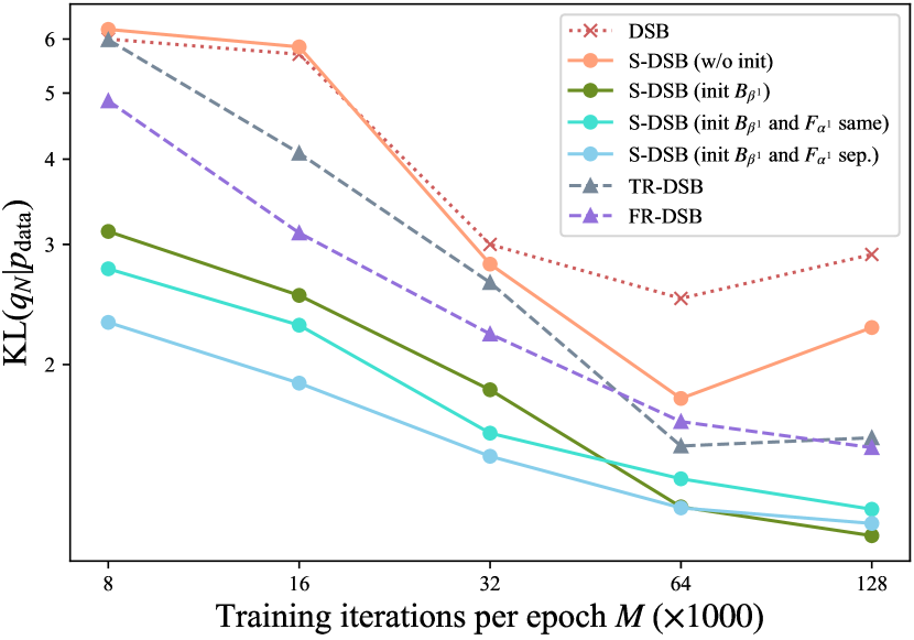
Figure 3: Evolution of performance with the increase of training iterations per epoch.
Refer to caption
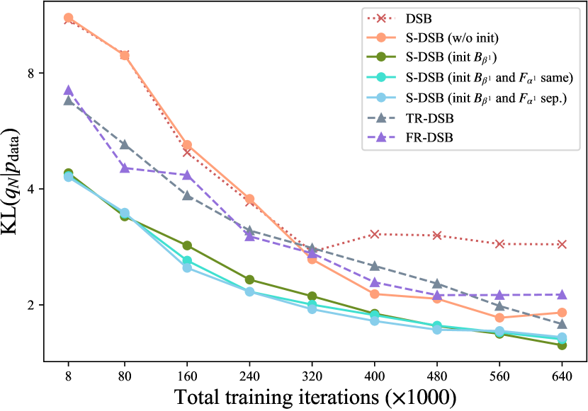
Figure 4: Evolution of performance with the increase of total training iterations.
Refer to caption
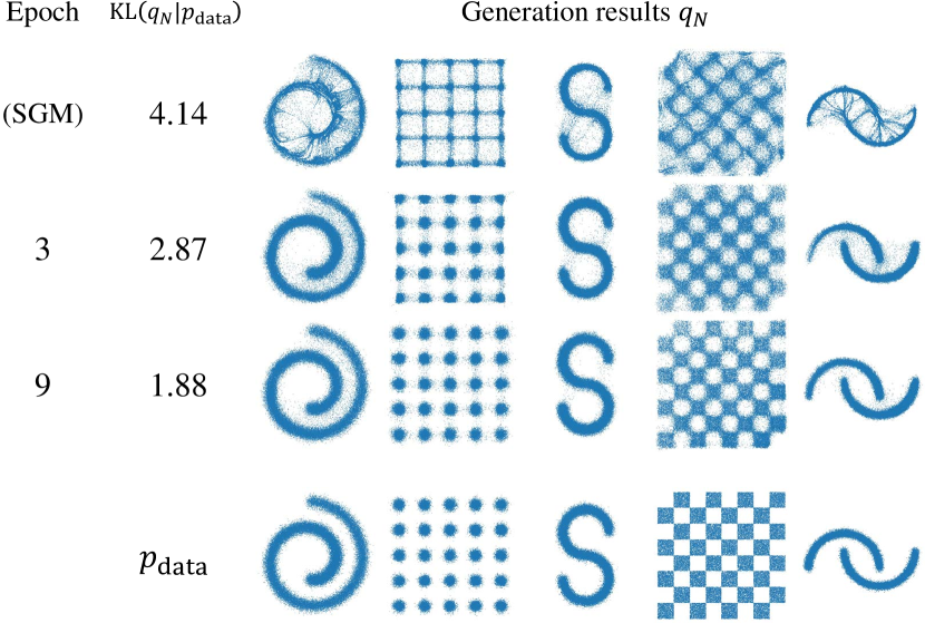
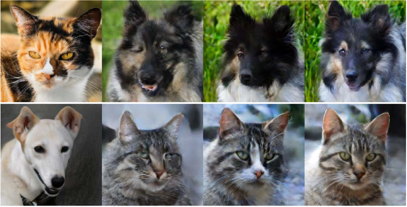
Figure 5: Improving pretrained SGM with S-DSB. First row illustrates the results of converged SGMs. KL divergences KL(qN|pdata)KLconditionalsubscript𝑞𝑁subscript𝑝data\textup{KL}(q_{N}|p_{\textup{data}}) measure the average generation performance of each rows.
Refer to caption
(a) Dog\rightarrowCat
Refer to caption
(b) Cat\rightarrowDog
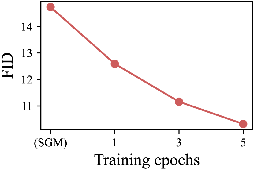
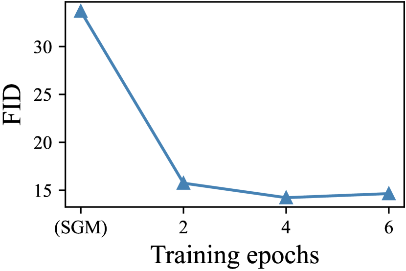
Figure 6: FID comparison of image translation on the AFHQ dataset.

We explore several critical factors that may impact the convergence of DSB, including training iterations per epoch M𝑀M, and the overall training iterations. To gauge convergence, we measured the KL divergence between the output of the backward networks and the real data distribution pdatasubscript𝑝datap_{\textup{data}}. As depicted in Figure 4, we subject all configurations to training over 101010 epochs. When M𝑀M is low, the DSB training fails to converge. As M𝑀M increases, the optimization process gradually approaches Equation 9, ultimately yielding improved final performance.

Figure 4 elucidates the enhancement of sample quality throughout the training duration. We set the default M𝑀M as 32K32𝐾32K. We note that the performance of DSB stops improving after 320K iterations. Conversely, both our S-DSB and R-DSB demonstrate consistent improvements. Moreover, even with random initialization, R-DSB surpasses the vanilla DSB in terms of sample quality.
Refer to caption
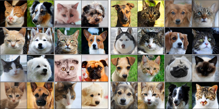
Figure 7: Generated samples on unpaired dog \leftrightarrow cat translation. Left: cat to dog; right: dog to cat. We observe that DSB could preserve pose and texture to a certain extent.

5.3 Improving SGM

Refer to caption
Figure 8: From left to right: input images, results from Flow Matching model, DSB 2-th epoch, and DSB 6-th epoch.

As discussed in Section 3.3, the simplified training objective in Equation 14 enables leveraging a pretrained SGM as the initial epoch for S-DSB and further improves it. In Figure 6, we first train diffusion models on various data distributions until convergence, and then employ these models as the starting point of S-DSB training. As depicted, the initial performance is suboptimal, with visually discernible artifacts presented in generated samples. However, after few epochs of S-DSB training, the sample quality is greatly improved. With continued training, the results progressively approximate the ground truths.

Additionally, we conducted validation on the AFHQ [12] dataset to transfer between dog and cat subsets. We utilized a pretrained Flow Matching (FM) [31] model as our initial model and applied Terminal Reparameterization to train the DSB. Given that FM constrains ppriorsubscript𝑝priorp_{\textup{prior}} to be Gaussian, it is understandable that the generated results may not be sufficiently good. As demonstrated in Figure 6 and Figure 8, our model is capable of progressively generating improved results. This further corroborates the efficacy of DSB in enhancing pretrained SGMs. We provide more translation results in Figure 7, which illustrate our method is capable of producing results with rich details and realistic textures.

5.4 γ𝛾\gamma term in DSB

Refer to caption
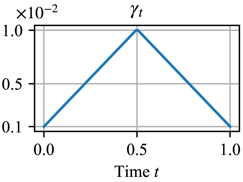
Figure 9: Linear symmetrical schedule for γtsubscript𝛾𝑡\gamma_{t}.

We adopt a symmetrical schedule for γtsubscript𝛾𝑡\gamma_{t} in our experiments, with values that linearly ascend from 103superscript10310^{-3} at both sides to 102superscript10210^{-2} at the center, as depicted in Figure 9. To examine the influence of γ𝛾\gamma, we present visualizations of two transformation trajectories from cat to dog under varying γtsubscript𝛾𝑡\gamma_{t} settings in Figure 10. Our observations indicate that a smaller γtsubscript𝛾𝑡\gamma_{t} tends to preserve more information throughout the trajectory, such as pose and color, whereas a larger γtsubscript𝛾𝑡\gamma_{t} can potentially lead to high-quality generated results.
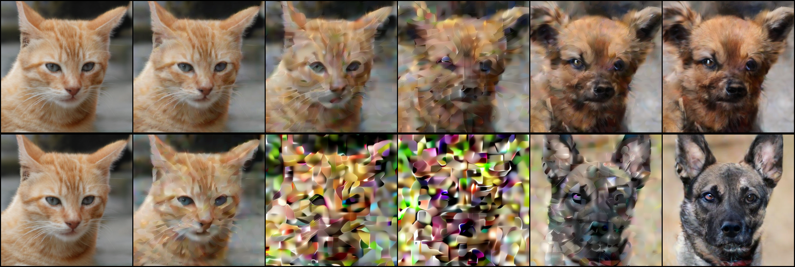
Refer to caption
Figure 10: Generation trajectories with different γtsubscript𝛾𝑡\gamma_{t}. Taking the same cat image as input, the trajectory with smaller γtsubscript𝛾𝑡\gamma_{t} can retain more details, such as pose and color. Above: γtlinear(104,103)subscript𝛾𝑡linearsuperscript104superscript103\gamma_{t}\in\text{linear}(10^{-4},10^{-3}). Below: γtlinear(103,102)subscript𝛾𝑡linearsuperscript103superscript102\gamma_{t}\in\text{linear}(10^{-3},10^{-2}).

6 Conclusion and Future Prospects

This paper proposes Simplified Diffusion Schrödinger Bridge (S-DSB), which unifies the training objectives of Diffusion Schrödinger Bridge (DSB) and Score-based generative models (SGMs). By leveraging SGMs as initialization, S-DSB achieves faster convergence and improved performance. The iterative refinement process inherent in DSB further enhances the outcomes of SGM. Our investigation delves deeply into the practical training of DSB, identifying critical factors that influence its success. Moreover, we introduce reparameterization techniques tailored for DSB that yield superior performance in real-world applications.

The authors firmly believe that approaches based on the Schrödinger Bridge problem represent the forward path for future generative models, as previous studies [13, 45] have unveiled its close connection with the optimal transport theory. Consequently, DSB has the theoretical potential to possess stronger generation capabilities and a deeper understanding of semantics. However, the authors acknowledge that the current DSB may still lag behind SGMs due to the complexity of its training process or a lack of effective reparameterization strategy to alleviate difficulties encountered during network training. This paper makes exploratory strides toward this goal and hopes to inspire future works.

References

  • [1] Video generation models as world simulators. https://openai.com/research/video-generation-models-as-world-simulators, accessed: 2024-03-01
  • [2] Anderson, B.D.: Reverse-time diffusion equation models. Stochastic Processes and their Applications 12(3), 313–326 (1982)
  • [3] Balaji, Y., Nah, S., Huang, X., Vahdat, A., Song, J., Kreis, K., Aittala, M., Aila, T., Laine, S., Catanzaro, B., et al.: ediffi: Text-to-image diffusion models with an ensemble of expert denoisers. arXiv preprint arXiv:2211.01324 (2022)
  • [4] Bernton, E., Heng, J., Doucet, A., Jacob, P.E.: Schrödinger bridge samplers. arXiv preprint arXiv:1912.13170 (2019)
  • [5] Blattmann, A., Dockhorn, T., Kulal, S., Mendelevitch, D., Kilian, M., Lorenz, D., Levi, Y., English, Z., Voleti, V., Letts, A., et al.: Stable video diffusion: Scaling latent video diffusion models to large datasets. arXiv preprint arXiv:2311.15127 (2023)
  • [6] Caluya, K.F., Halder, A.: Wasserstein proximal algorithms for the schrödinger bridge problem: Density control with nonlinear drift. IEEE Transactions on Automatic Control 67(3), 1163–1178 (2021)
  • [7] Cattiaux, P., Conforti, G., Gentil, I., Léonard, C.: Time reversal of diffusion processes under a finite entropy condition. arXiv preprint arXiv:2104.07708 (2021)
  • [8] Chen, T.: On the importance of noise scheduling for diffusion models. arXiv preprint arXiv:2301.10972 (2023)
  • [9] Chen, Y., Georgiou, T., Pavon, M.: Entropic and displacement interpolation: a computational approach using the hilbert metric. SIAM Journal on Applied Mathematics 76(6), 2375–2396 (2016)
  • [10] Chen, Y., Georgiou, T.T., Pavon, M.: Optimal transport in systems and control. Annual Review of Control, Robotics, and Autonomous Systems 4 (2021)
  • [11] Chen, Z., He, G., Zheng, K., Tan, X., Zhu, J.: Schrodinger bridges beat diffusion models on text-to-speech synthesis. arXiv preprint arXiv:2312.03491 (2023)
  • [12] Choi, Y., Uh, Y., Yoo, J., Ha, J.W.: Stargan v2: Diverse image synthesis for multiple domains. In: Proceedings of the IEEE/CVF conference on computer vision and pattern recognition. pp. 8188–8197 (2020)
  • [13] De Bortoli, V., Thornton, J., Heng, J., Doucet, A.: Diffusion schrödinger bridge with applications to score-based generative modeling. Advances in Neural Information Processing Systems 34, 17695–17709 (2021)
  • [14] Dhariwal, P., Nichol, A.: Diffusion models beat gans on image synthesis. Advances in neural information processing systems 34, 8780–8794 (2021)
  • [15] Finlay, C., Gerolin, A., Oberman, A.M., Pooladian, A.A.: Learning normalizing flows from entropy-kantorovich potentials. arXiv preprint arXiv:2006.06033 (2020)
  • [16] Föllmer, H.: An entropy approach to the time reversal of diffusion processes. In: Stochastic Differential Systems: Filtering and Control, pp. 156–163. Springer (1985)
  • [17] Föllmer, H.: Random fields and diffusion processes. In: École d’Été de Probabilités de Saint-Flour XV–XVII, 1985–87, pp. 101–203. Springer (1988)
  • [18] Fortet, R.: Résolution d’un système d’équations de M. Schrödinger. Journal de Mathématiques Pures et Appliqués 1, 83–105 (1940)
  • [19] Gu, J., Zhai, S., Zhang, Y., Bautista, M.A., Susskind, J.: f-dm: A multi-stage diffusion model via progressive signal transformation. International Conference on Learning Representations (2021)
  • [20] Gu, S., Chen, D., Bao, J., Wen, F., Zhang, B., Chen, D., Yuan, L., Guo, B.: Vector quantized diffusion model for text-to-image synthesis. In: Proceedings of the IEEE/CVF Conference on Computer Vision and Pattern Recognition. pp. 10696–10706 (2022)
  • [21] Hang, T., Gu, S., Li, C., Bao, J., Chen, D., Hu, H., Geng, X., Guo, B.: Efficient diffusion training via min-snr weighting strategy. arXiv preprint arXiv:2303.09556 (2023)
  • [22] Haussmann, U.G., Pardoux, E.: Time reversal of diffusions. The Annals of Probability 14(4), 1188–1205 (1986)
  • [23] Ho, J., Chan, W., Saharia, C., Whang, J., Gao, R., Gritsenko, A., Kingma, D.P., Poole, B., Norouzi, M., Fleet, D.J., et al.: Imagen video: High definition video generation with diffusion models. arXiv preprint arXiv:2210.02303 (2022)
  • [24] Ho, J., Jain, A., Abbeel, P.: Denoising diffusion probabilistic models. Advances in neural information processing systems 33, 6840–6851 (2020)
  • [25] Hyvärinen, A., Dayan, P.: Estimation of non-normalized statistical models by score matching. Journal of Machine Learning Research 6(4) (2005)
  • [26] Jun, H., Nichol, A.: Shap-e: Generating conditional 3d implicit functions. arXiv preprint arXiv:2305.02463 (2023)
  • [27] Karras, T., Aittala, M., Aila, T., Laine, S.: Elucidating the design space of diffusion-based generative models. Advances in Neural Information Processing Systems 35, 26565–26577 (2022)
  • [28] Kullback, S.: Probability densities with given marginals. The Annals of Mathematical Statistics 39(4), 1236–1243 (1968)
  • [29] Léonard, C.: A survey of the Schrödinger problem and some of its connections with optimal transport. Discrete & Continuous Dynamical Systems-A 34(4), 1533–1574 (2014)
  • [30] Lin, S., Liu, B., Li, J., Yang, X.: Common diffusion noise schedules and sample steps are flawed. In: Proceedings of the IEEE/CVF Winter Conference on Applications of Computer Vision. pp. 5404–5411 (2024)
  • [31] Lipman, Y., Chen, R.T., Ben-Hamu, H., Nickel, M., Le, M.: Flow matching for generative modeling. International Conference on Learning Representations (2023)
  • [32] Liu, G.H., Vahdat, A., Huang, D.A., Theodorou, E.A., Nie, W., Anandkumar, A.: I 2 sb: Image-to-image schrödinger bridge. International Conference on Machine Learning (2023)
  • [33] Liu, X., Gong, C., Liu, Q.: Flow straight and fast: Learning to generate and transfer data with rectified flow. International Conference on Learning Representations (2023)
  • [34] Liu, Z., Luo, P., Wang, X., Tang, X.: Deep learning face attributes in the wild. In: Proceedings of International Conference on Computer Vision (ICCV) (December 2015)
  • [35] Nelson, E.: Dynamical theories of brownian motion (1967)
  • [36] Nichol, A., Jun, H., Dhariwal, P., Mishkin, P., Chen, M.: Point-e: A system for generating 3d point clouds from complex prompts. arXiv preprint arXiv:2212.08751 (2022)
  • [37] Pavon, M., Trigila, G., Tabak, E.G.: The data-driven schrödinger bridge. Communications on Pure and Applied Mathematics 74(7), 1545–1573 (2021)
  • [38] Ramesh, A., Dhariwal, P., Nichol, A., Chu, C., Chen, M.: Hierarchical text-conditional image generation with clip latents. arXiv preprint arXiv:2204.06125 1(2),  3 (2022)
  • [39] Ramesh, A., Pavlov, M., Goh, G., Gray, S., Voss, C., Radford, A., Chen, M., Sutskever, I.: Zero-shot text-to-image generation. In: International Conference on Machine Learning. pp. 8821–8831. PMLR (2021)
  • [40] Rombach, R., Blattmann, A., Lorenz, D., Esser, P., Ommer, B.: High-resolution image synthesis with latent diffusion models. In: Proceedings of the IEEE/CVF conference on computer vision and pattern recognition. pp. 10684–10695 (2022)
  • [41] Rüschendorf, L., Thomsen, W.: Note on the schrödinger equation and i-projections. Statistics & probability letters 17(5), 369–375 (1993)
  • [42] Ruschendorf, L., et al.: Convergence of the iterative proportional fitting procedure. The Annals of Statistics 23(4), 1160–1174 (1995)
  • [43] Salimans, T., Ho, J.: Progressive distillation for fast sampling of diffusion models. International Conference on Learning Representations (2022)
  • [44] Schrödinger, E.: Sur la théorie relativiste de l’électron et l’interprétation de la mécanique quantique. Annales de l’Institut Henri Poincaré 2(4), 269–310 (1932)
  • [45] Shi, Y., De Bortoli, V., Campbell, A., Doucet, A.: Diffusion schrödinger bridge matching. Advances in Neural Information Processing Systems 36 (2024)
  • [46] Sohl-Dickstein, J., Weiss, E., Maheswaranathan, N., Ganguli, S.: Deep unsupervised learning using nonequilibrium thermodynamics. In: International conference on machine learning. pp. 2256–2265. PMLR (2015)
  • [47] Song, J., Meng, C., Ermon, S.: Denoising diffusion implicit models. International Conference on Learning Representations (2021)
  • [48] Song, Y., Ermon, S.: Generative modeling by estimating gradients of the data distribution. Advances in neural information processing systems 32 (2019)
  • [49] Song, Y., Sohl-Dickstein, J., Kingma, D.P., Kumar, A., Ermon, S., Poole, B.: Score-based generative modeling through stochastic differential equations. International Conference on Learning Representations (2021)
  • [50] Tang, Z., Gu, S., Wang, C., Zhang, T., Bao, J., Chen, D., Guo, B.: Volumediffusion: Flexible text-to-3d generation with efficient volumetric encoder. arXiv preprint arXiv:2312.11459 (2023)
  • [51] Tong, A., Malkin, N., Huguet, G., Zhang, Y., Rector-Brooks, J., Fatras, K., Wolf, G., Bengio, Y.: Improving and generalizing flow-based generative models with minibatch optimal transport. In: ICML Workshop on New Frontiers in Learning, Control, and Dynamical Systems (2023)
  • [52] Vincent, P.: A connection between score matching and denoising autoencoders. Neural Computation 23(7), 1661–1674 (2011)
  • [53] Zhu, J.Y., Park, T., Isola, P., Efros, A.A.: Unpaired image-to-image translation using cycle-consistent adversarial networks. In: Proceedings of the IEEE international conference on computer vision. pp. 2223–2232 (2017)

Appendix 0.A Proof of Proposition 2

Proof

By asssumption, we have

(xk+1+Fkn(xk)Fkn(xk+1))xksubscript𝑥𝑘1superscriptsubscript𝐹𝑘𝑛subscript𝑥𝑘superscriptsubscript𝐹𝑘𝑛subscript𝑥𝑘1subscript𝑥𝑘\displaystyle\ \left(x_{k+1}+F_{k}^{n}(x_{k})-F_{k}^{n}(x_{k+1})\right)-x_{k} (22)
=\displaystyle= (xk+1+xk+γk+1fkn(xk)(xk+1+γk+1fkn(xk+1)))xksubscript𝑥𝑘1subscript𝑥𝑘subscript𝛾𝑘1superscriptsubscript𝑓𝑘𝑛subscript𝑥𝑘subscript𝑥𝑘1subscript𝛾𝑘1superscriptsubscript𝑓𝑘𝑛subscript𝑥𝑘1subscript𝑥𝑘\displaystyle\ \left(x_{k+1}+x_{k}+\gamma_{k+1}f_{k}^{n}(x_{k})-\left(x_{k+1}+\gamma_{k+1}f_{k}^{n}(x_{k+1})\right)\right)-x_{k}
=\displaystyle= (xk+γk+1fkn(xk)γk+1fkn(xk+1))xksubscript𝑥𝑘subscript𝛾𝑘1superscriptsubscript𝑓𝑘𝑛subscript𝑥𝑘subscript𝛾𝑘1superscriptsubscript𝑓𝑘𝑛subscript𝑥𝑘1subscript𝑥𝑘\displaystyle\ \left(x_{k}+\gamma_{k+1}f_{k}^{n}(x_{k})-\gamma_{k+1}f_{k}^{n}(x_{k+1})\right)-x_{k}
=\displaystyle= γk+1fkn(xk)γk+1fkn(xk+1)subscript𝛾𝑘1superscriptsubscript𝑓𝑘𝑛subscript𝑥𝑘subscript𝛾𝑘1superscriptsubscript𝑓𝑘𝑛subscript𝑥𝑘1\displaystyle\ \gamma_{k+1}f_{k}^{n}(x_{k})-\gamma_{k+1}f_{k}^{n}(x_{k+1})
=\displaystyle= fkn(xk)fkn(xk+1)superscriptsubscript𝑓𝑘𝑛subscript𝑥𝑘superscriptsubscript𝑓𝑘𝑛subscript𝑥𝑘1\displaystyle\ f_{k}^{n}(x_{k})-f_{k}^{n}(x_{k+1})
\displaystyle\approx 0,0\displaystyle\ 0,

and thus Bk+1nBk+1nsuperscriptsubscriptsuperscriptsubscript𝐵𝑘1𝑛subscriptsuperscriptsubscript𝐵𝑘1𝑛\mathcal{L}_{B_{k+1}^{n}}^{{}^{\prime}}\approx\mathcal{L}_{B_{k+1}^{n}}. Fkn+1Fkn+1superscriptsubscriptsuperscriptsubscript𝐹𝑘𝑛1subscriptsuperscriptsubscript𝐹𝑘𝑛1\mathcal{L}_{F_{k}^{n+1}}^{{}^{\prime}}\approx\mathcal{L}_{F_{k}^{n+1}} can also be proved likewise.

Appendix 0.B Proof of Proposition 19

0.B.1 Continuous-time DSB

To prove Proposition 19, we first introduce continuous-time DSB. Given a reference measure 𝒫(𝒞)𝒫𝒞\mathbb{P}\in\mathscr{P}(\mathcal{C}), the continuous-time SB problem aims to find

Π=argmin{KL(Π|):Π𝒫(𝒞),Π0=pdata,ΠT=pprior}.superscriptΠ:KLconditionalΠformulae-sequenceΠ𝒫𝒞formulae-sequencesubscriptΠ0subscript𝑝datasubscriptΠ𝑇subscript𝑝prior\displaystyle\mathrm{\Pi}^{*}=\arg\min\{\textup{KL}(\mathrm{\Pi}|\mathbb{P}):\mathrm{\Pi}\in\mathscr{P}(\mathcal{C}),\mathrm{\Pi}_{0}=p_{\textup{data}},\mathrm{\Pi}_{T}=p_{\textup{prior}}\}. (23)

Similar to Equation 8, continuous-time IPF iterations (Πn)nsubscriptsuperscriptΠ𝑛𝑛(\mathrm{\Pi}^{n})_{n\in\mathbb{N}} where Π0=superscriptΠ0\mathrm{\Pi}^{0}=\mathbb{P} for any n𝑛n\in\mathbb{N} can be defined in continuous time as

Π2n+1superscriptΠ2𝑛1\displaystyle\mathrm{\Pi}^{2n+1} =argmin{KL(Π|Π2n):Π𝒫(𝒞),ΠT=pprior},absent:KLconditionalΠsuperscriptΠ2𝑛formulae-sequenceΠ𝒫𝒞subscriptΠ𝑇subscript𝑝prior\displaystyle=\arg\min\{\textup{KL}(\mathrm{\Pi}|\mathrm{\Pi}^{2n}):\mathrm{\Pi}\in\mathscr{P}(\mathcal{C}),\mathrm{\Pi}_{T}=p_{\textup{prior}}\}, (24)
Π2n+2superscriptΠ2𝑛2\displaystyle\mathrm{\Pi}^{2n+2} =argmin{KL(Π|Π2n+1):Π𝒫(𝒞),Π0=pdata}.absent:KLconditionalΠsuperscriptΠ2𝑛1formulae-sequenceΠ𝒫𝒞subscriptΠ0subscript𝑝data\displaystyle=\arg\min\{\textup{KL}(\mathrm{\Pi}|\mathrm{\Pi}^{2n+1}):\mathrm{\Pi}\in\mathscr{P}(\mathcal{C}),\mathrm{\Pi}_{0}=p_{\textup{data}}\}.

DSB partitions the continuous time horizon [0,T]0𝑇[0,T] into N+1𝑁1N+1 discrete timesteps {γ¯0,γ¯1,,γ¯N}subscript¯𝛾0subscript¯𝛾1subscript¯𝛾𝑁\{\bar{\gamma}_{0},\bar{\gamma}_{1},\ldots,\bar{\gamma}_{N}\} where γ¯k=n=1kγnsubscript¯𝛾𝑘superscriptsubscript𝑛1𝑘subscript𝛾𝑛\bar{\gamma}_{k}=\sum_{n=1}^{k}\gamma_{n}, γ¯0=0subscript¯𝛾00\bar{\gamma}_{0}=0 and γ¯N=Tsubscript¯𝛾𝑁𝑇\bar{\gamma}_{N}=T. The forward process is pγ¯k+1|γ¯kn=𝒩(xγ¯k+1;xγ¯k+γk+1fγ¯kn(xγ¯k),2γk+1𝐈)superscriptsubscript𝑝conditionalsubscript¯𝛾𝑘1subscript¯𝛾𝑘𝑛𝒩subscript𝑥subscript¯𝛾𝑘1subscript𝑥subscript¯𝛾𝑘subscript𝛾𝑘1superscriptsubscript𝑓subscript¯𝛾𝑘𝑛subscript𝑥subscript¯𝛾𝑘2subscript𝛾𝑘1𝐈p_{\bar{\gamma}_{k+1}|\bar{\gamma}_{k}}^{n}=\mathcal{N}\left(x_{\bar{\gamma}_{k+1}};x_{\bar{\gamma}_{k}}+\gamma_{k+1}f_{\bar{\gamma}_{k}}^{n}(x_{\bar{\gamma}_{k}}),2\gamma_{k+1}\mathbf{I}\right) and the backward process is qγ¯k|γ¯k+1n=𝒩(xγ¯k;xγ¯k+1+γk+1bγ¯k+1n(xγ¯k+1),2γk+1𝐈)superscriptsubscript𝑞conditionalsubscript¯𝛾𝑘subscript¯𝛾𝑘1𝑛𝒩subscript𝑥subscript¯𝛾𝑘subscript𝑥subscript¯𝛾𝑘1subscript𝛾𝑘1superscriptsubscript𝑏subscript¯𝛾𝑘1𝑛subscript𝑥subscript¯𝛾𝑘12subscript𝛾𝑘1𝐈q_{\bar{\gamma}_{k}|\bar{\gamma}_{k+1}}^{n}=\mathcal{N}\left(x_{\bar{\gamma}_{k}};x_{\bar{\gamma}_{k+1}}+\gamma_{k+1}b_{\bar{\gamma}_{k+1}}^{n}(x_{\bar{\gamma}_{k+1}}),2\gamma_{k+1}\mathbf{I}\right), where fγ¯kn(xγ¯k)superscriptsubscript𝑓subscript¯𝛾𝑘𝑛subscript𝑥subscript¯𝛾𝑘f_{\bar{\gamma}_{k}}^{n}(x_{\bar{\gamma}_{k}}) and bγ¯k+1n(xγ¯k+1)superscriptsubscript𝑏subscript¯𝛾𝑘1𝑛subscript𝑥subscript¯𝛾𝑘1b_{\bar{\gamma}_{k+1}}^{n}(x_{\bar{\gamma}_{k+1}}) are drift terms, and pnsuperscript𝑝𝑛p^{n} and qnsuperscript𝑞𝑛q^{n} are discretizations of Π2nsuperscriptΠ2𝑛\mathrm{\Pi}^{2n} and Π2n+1superscriptΠ2𝑛1\mathrm{\Pi}^{2n+1}, respectively. DSB uses two neural networks to approximate Bβn(γ¯k,x)Bγ¯kn(x)=x+γ¯kbγ¯kn(x)subscript𝐵superscript𝛽𝑛subscript¯𝛾𝑘𝑥superscriptsubscript𝐵subscript¯𝛾𝑘𝑛𝑥𝑥subscript¯𝛾𝑘superscriptsubscript𝑏subscript¯𝛾𝑘𝑛𝑥B_{\beta^{n}}(\bar{\gamma}_{k},x)\approx B_{\bar{\gamma}_{k}}^{n}(x)=x+\bar{\gamma}_{k}b_{\bar{\gamma}_{k}}^{n}(x) and Fαn(γ¯k,x)Fγ¯kn(x)=x+γ¯k+1fγ¯kn(x)subscript𝐹superscript𝛼𝑛subscript¯𝛾𝑘𝑥superscriptsubscript𝐹subscript¯𝛾𝑘𝑛𝑥𝑥subscript¯𝛾𝑘1superscriptsubscript𝑓subscript¯𝛾𝑘𝑛𝑥F_{\alpha^{n}}(\bar{\gamma}_{k},x)\approx F_{\bar{\gamma}_{k}}^{n}(x)=x+\bar{\gamma}_{k+1}f_{\bar{\gamma}_{k}}^{n}(x).

0.B.2 Posterior estimation

First, we introduce some notations in continuous-time SDEs. We rewrite Equation 11 as

d𝐗tdsubscript𝐗𝑡\displaystyle\mathrm{d}\mathbf{X}_{t} =(f(𝐗t,t)+g2(t)log𝚿(𝐗t,t))dt+g(t)d𝐖t,X0pdataformulae-sequenceabsent𝑓subscript𝐗𝑡𝑡superscript𝑔2𝑡𝚿subscript𝐗𝑡𝑡d𝑡𝑔𝑡dsubscript𝐖𝑡similar-tosubscript𝑋0subscript𝑝data\displaystyle=\left(f(\mathbf{X}_{t},t)+g^{2}(t)\nabla\log\mathbf{\Psi}(\mathbf{X}_{t},t)\right)\mathrm{d}t+g(t)\mathrm{d}\mathbf{W}_{t},X_{0}\sim p_{\textup{data}}
:=h(𝐗t,t)dt+g(t)d𝐖t,X0pdata,formulae-sequenceassignabsentsubscript𝐗𝑡𝑡d𝑡𝑔𝑡dsubscript𝐖𝑡similar-tosubscript𝑋0subscript𝑝data\displaystyle:=h(\mathbf{X}_{t},t)\mathrm{d}t+g(t)\mathrm{d}\mathbf{W}_{t},X_{0}\sim p_{\textup{data}}, (25a)
d𝐗tdsubscript𝐗𝑡\displaystyle\mathrm{d}\mathbf{X}_{t} =(f(𝐗t,t)g2(t)log𝚿^(𝐗t,t))dt+g(t)d𝐖¯t,X0pdataformulae-sequenceabsent𝑓subscript𝐗𝑡𝑡superscript𝑔2𝑡^𝚿subscript𝐗𝑡𝑡d𝑡𝑔𝑡dsubscript¯𝐖𝑡similar-tosubscript𝑋0subscript𝑝data\displaystyle=\left(f(\mathbf{X}_{t},t)-g^{2}(t)\nabla\log\mathbf{\hat{\Psi}}(\mathbf{X}_{t},t)\right)\mathrm{d}t+g(t)\mathrm{d}\mathbf{\bar{W}}_{t},X_{0}\sim p_{\textup{data}}
:=l(𝐗t,t)dt+g(t)d𝐖¯t,X1pprior,formulae-sequenceassignabsent𝑙subscript𝐗𝑡𝑡d𝑡𝑔𝑡dsubscript¯𝐖𝑡similar-tosubscript𝑋1subscript𝑝prior\displaystyle:=l(\mathbf{X}_{t},t)\mathrm{d}t+g(t)\mathrm{d}\mathbf{\bar{W}}_{t},X_{1}\sim p_{\textup{prior}}, (25b)

where h(𝐗t,t)subscript𝐗𝑡𝑡h(\mathbf{X}_{t},t) and l(𝐗t,t)𝑙subscript𝐗𝑡𝑡l(\mathbf{X}_{t},t) are drift terms. Given the forward trajectory x0:Npn(x0:N)similar-tosubscript𝑥:0𝑁superscript𝑝𝑛subscript𝑥:0𝑁x_{0:N}\sim p^{n}(x_{0:N}) and the backward trajectory x0:Nqn(x0:N)similar-tosubscriptsuperscript𝑥:0𝑁superscript𝑞𝑛subscript𝑥:0𝑁x^{\prime}_{0:N}\sim q^{n}(x_{0:N}), {xγ¯i:=xi}i=0Nsuperscriptsubscriptassignsubscript𝑥subscript¯𝛾𝑖subscript𝑥𝑖𝑖0𝑁\{x_{\bar{\gamma}_{i}}:=x_{i}\}_{i=0}^{N} and {xγ¯i:=xi}i=0Nsuperscriptsubscriptassignsubscriptsuperscript𝑥subscript¯𝛾𝑖subscriptsuperscript𝑥𝑖𝑖0𝑁\{x^{\prime}_{\bar{\gamma}_{i}}:=x^{\prime}_{i}\}_{i=0}^{N} denote the trajectories of Equation 25a and Equation 25b at time {γ¯0,γ¯1,,γ¯N}subscript¯𝛾0subscript¯𝛾1subscript¯𝛾𝑁\{\bar{\gamma}_{0},\bar{\gamma}_{1},\ldots,\bar{\gamma}_{N}\}, respectively. For simplicity, we denote the integration abh(𝐗t,t)superscriptsubscript𝑎𝑏subscript𝐗𝑡𝑡\int_{a}^{b}h(\mathbf{X}_{t},t) and abl(𝐗t,t)superscriptsubscript𝑎𝑏𝑙subscript𝐗𝑡𝑡\int_{a}^{b}l(\mathbf{X}_{t},t) as h~(a,b)~𝑎𝑏\tilde{h}(a,b) and l~(a,b)~𝑙𝑎𝑏\tilde{l}(a,b), respectively.

Here we give a full version of Proposition 19:

Proposition 4

Assume γ¯N=1subscript¯𝛾𝑁1\bar{\gamma}_{N}=1. Given the forward and backward trajectories x0:Npn(x0:N)=p0n(x0)k=0N1pk+1|kn(xk+1|xk)similar-tosubscript𝑥:0𝑁superscript𝑝𝑛subscript𝑥:0𝑁superscriptsubscript𝑝0𝑛subscript𝑥0superscriptsubscriptproduct𝑘0𝑁1superscriptsubscript𝑝𝑘conditional1𝑘𝑛conditionalsubscript𝑥𝑘1subscript𝑥𝑘x_{0:N}\sim p^{n}(x_{0:N})=p_{0}^{n}(x_{0})\prod_{k=0}^{N-1}p_{k+1|k}^{n}(x_{k+1}|x_{k}) and x0:Nqn(x0:N)=qNn(xN)k=0N1pk|k+1n(xk|xk+1)similar-tosuperscriptsubscript𝑥:0𝑁superscript𝑞𝑛subscript𝑥:0𝑁superscriptsubscript𝑞𝑁𝑛subscript𝑥𝑁superscriptsubscriptproduct𝑘0𝑁1superscriptsubscript𝑝conditional𝑘𝑘1𝑛conditionalsubscript𝑥𝑘subscript𝑥𝑘1x_{0:N}^{\prime}\sim q^{n}(x_{0:N})=q_{N}^{n}(x_{N})\prod_{k=0}^{N-1}p_{k|k+1}^{n}(x_{k}|x_{k+1}). Assume ft(𝐗t)=α𝐗tsubscript𝑓𝑡subscript𝐗𝑡𝛼subscript𝐗𝑡f_{t}(\mathbf{X}_{t})=-\alpha\mathbf{X}_{t}, g(t)=2𝑔𝑡2g(t)=\sqrt{2},

1γ¯kh~(0,γ¯k)1γ¯k+1h~(0,γ¯k+1),11γ¯kl~(γ¯k,1)11γ¯k+1l~(γ¯k+1,1).formulae-sequence1subscript¯𝛾𝑘~0subscript¯𝛾𝑘1subscript¯𝛾𝑘1~0subscript¯𝛾𝑘111subscript¯𝛾𝑘~𝑙subscript¯𝛾𝑘111subscript¯𝛾𝑘1~𝑙subscript¯𝛾𝑘11\displaystyle\frac{1}{\bar{\gamma}_{k}}\tilde{h}(0,\bar{\gamma}_{k})\approx\frac{1}{\bar{\gamma}_{k+1}}\tilde{h}(0,\bar{\gamma}_{k+1}),\frac{1}{1-\bar{\gamma}_{k}}\tilde{l}(\bar{\gamma}_{k},1)\approx\frac{1}{1-\bar{\gamma}_{k+1}}\tilde{l}(\bar{\gamma}_{k+1},1). (26)

We have

qk|k+1n(xk|xk+1)pk|k+1,0n(xk|xk+1,x0)=𝒩(xk;μk+1n(xk+1,x0),σk+1𝐈),superscriptsubscript𝑞conditional𝑘𝑘1𝑛conditionalsubscript𝑥𝑘subscript𝑥𝑘1superscriptsubscript𝑝conditional𝑘𝑘10𝑛conditionalsubscript𝑥𝑘subscript𝑥𝑘1subscript𝑥0𝒩subscript𝑥𝑘superscriptsubscript𝜇𝑘1𝑛subscript𝑥𝑘1subscript𝑥0subscript𝜎𝑘1𝐈\displaystyle q_{k|k+1}^{n}(x_{k}|x_{k+1})\approx p_{k|k+1,0}^{n}(x_{k}|x_{k+1},x_{0})=\mathcal{N}(x_{k};\mu_{k+1}^{n}(x_{k+1},x_{0}),\sigma_{k+1}\mathbf{I}), (27a)
pk+1|kn+1(xk+1|xk)qk+1|k,Nn(xk+1|xk,xN)=𝒩(xk+1;μ~kn(xk,xN),σ~k+1𝐈),superscriptsubscript𝑝𝑘conditional1𝑘𝑛1conditionalsubscript𝑥𝑘1subscript𝑥𝑘superscriptsubscript𝑞𝑘conditional1𝑘𝑁𝑛conditionalsuperscriptsubscript𝑥𝑘1superscriptsubscript𝑥𝑘superscriptsubscript𝑥𝑁𝒩superscriptsubscript𝑥𝑘1superscriptsubscript~𝜇𝑘𝑛superscriptsubscript𝑥𝑘superscriptsubscript𝑥𝑁subscript~𝜎𝑘1𝐈\displaystyle p_{k+1|k}^{n+1}(x_{k+1}|x_{k})\approx q_{k+1|k,N}^{n}(x_{k+1}^{\prime}|x_{k}^{\prime},x_{N}^{\prime})=\mathcal{N}(x_{k+1}^{\prime};\tilde{\mu}_{k}^{n}(x_{k}^{\prime},x_{N}^{\prime}),\tilde{\sigma}_{k+1}\mathbf{I}), (27b)
μk+1n(xk+1,x0)xk+1+γk+1γ¯k+1(x0xk+1),σk+1=2γk+1γ¯kγ¯k+1,formulae-sequencesuperscriptsubscript𝜇𝑘1𝑛subscript𝑥𝑘1subscript𝑥0subscript𝑥𝑘1subscript𝛾𝑘1subscript¯𝛾𝑘1subscript𝑥0subscript𝑥𝑘1subscript𝜎𝑘12subscript𝛾𝑘1subscript¯𝛾𝑘subscript¯𝛾𝑘1\displaystyle\mu_{k+1}^{n}(x_{k+1},x_{0})\approx x_{k+1}+\frac{\gamma_{k+1}}{\bar{\gamma}_{k+1}}(x_{0}-x_{k+1}),\sigma_{k+1}=\frac{2\gamma_{k+1}\bar{\gamma}_{k}}{\bar{\gamma}_{k+1}}, (28a)
μ~kn(xk,xN)xk+γk+11γ¯k(xNxk),σ~k+1=2γk+1(1γ¯k+1)1γ¯k.formulae-sequencesubscriptsuperscript~𝜇𝑛𝑘superscriptsubscript𝑥𝑘superscriptsubscript𝑥𝑁superscriptsubscript𝑥𝑘subscript𝛾𝑘11subscript¯𝛾𝑘superscriptsubscript𝑥𝑁superscriptsubscript𝑥𝑘subscript~𝜎𝑘12subscript𝛾𝑘11subscript¯𝛾𝑘11subscript¯𝛾𝑘\displaystyle\tilde{\mu}^{n}_{k}(x_{k}^{\prime},x_{N}^{\prime})\approx x_{k}^{\prime}+\frac{\gamma_{k+1}}{1-\bar{\gamma}_{k}}(x_{N}^{\prime}-x_{k}^{\prime}),\tilde{\sigma}_{k+1}=\frac{2\gamma_{k+1}(1-\bar{\gamma}_{k+1})}{1-\bar{\gamma}_{k}}. (28b)

It is worth noticing that ft(𝐗t)=α𝐗tsubscript𝑓𝑡subscript𝐗𝑡𝛼subscript𝐗𝑡f_{t}(\mathbf{X}_{t})=-\alpha\mathbf{X}_{t} and g(t)=2𝑔𝑡2g(t)=\sqrt{2} are assumptions of the original DSB [13]. We prove Proposition 28 with the following lemmas.

Lemma 1

Given the forward and backward trajectories x0:Npn(x0:N)=p0n(x0)k=0N1pk+1|kn(xk+1|xk)similar-tosubscript𝑥:0𝑁superscript𝑝𝑛subscript𝑥:0𝑁superscriptsubscript𝑝0𝑛subscript𝑥0superscriptsubscriptproduct𝑘0𝑁1superscriptsubscript𝑝𝑘conditional1𝑘𝑛conditionalsubscript𝑥𝑘1subscript𝑥𝑘x_{0:N}\sim p^{n}(x_{0:N})=p_{0}^{n}(x_{0})\prod_{k=0}^{N-1}p_{k+1|k}^{n}(x_{k+1}|x_{k}) and x0:Nqn(x0:N)=qNn(xN)k=0N1pk|k+1n(xk|xk+1)similar-tosuperscriptsubscript𝑥:0𝑁superscript𝑞𝑛subscript𝑥:0𝑁superscriptsubscript𝑞𝑁𝑛subscript𝑥𝑁superscriptsubscriptproduct𝑘0𝑁1superscriptsubscript𝑝conditional𝑘𝑘1𝑛conditionalsubscript𝑥𝑘subscript𝑥𝑘1x_{0:N}^{\prime}\sim q^{n}(x_{0:N})=q_{N}^{n}(x_{N})\prod_{k=0}^{N-1}p_{k|k+1}^{n}(x_{k}|x_{k+1}). Suppose the IPF in Equation 24 achieve the optimal state. Then we have

qk|k+1n(xk|xk+1)pk|k+1,0n(xk|xk+1,x0),superscriptsubscript𝑞conditional𝑘𝑘1𝑛conditionalsubscript𝑥𝑘subscript𝑥𝑘1superscriptsubscript𝑝conditional𝑘𝑘10𝑛conditionalsubscript𝑥𝑘subscript𝑥𝑘1subscript𝑥0\displaystyle q_{k|k+1}^{n}(x_{k}|x_{k+1})\approx p_{k|k+1,0}^{n}(x_{k}|x_{k+1},x_{0}), (29a)
pk+1|kn+1(xk+1|xk)qk+1|k,Nn(xk+1|xk,xN).superscriptsubscript𝑝𝑘conditional1𝑘𝑛1conditionalsubscript𝑥𝑘1subscript𝑥𝑘superscriptsubscript𝑞𝑘conditional1𝑘𝑁𝑛conditionalsuperscriptsubscript𝑥𝑘1superscriptsubscript𝑥𝑘superscriptsubscript𝑥𝑁\displaystyle p_{k+1|k}^{n+1}(x_{k+1}|x_{k})\approx q_{k+1|k,N}^{n}(x_{k+1}^{\prime}|x_{k}^{\prime},x_{N}^{\prime}). (29b)
Proof

We first prove Equation 29a. In (2n+1)2𝑛1(2n+1)-th iteration, IPF aims to solve

KL(qn|pn)KLconditionalsuperscript𝑞𝑛superscript𝑝𝑛\displaystyle\textup{KL}\left(q^{n}|p^{n}\right) =𝔼qn(logqn(xN)k=0N1qn(xk|xk+1)pn(x0)pn(xN|x0)k=1N1pn(xk|xk+1,x0))absentsubscript𝔼superscript𝑞𝑛superscript𝑞𝑛subscript𝑥𝑁superscriptsubscriptproduct𝑘0𝑁1superscript𝑞𝑛conditionalsubscript𝑥𝑘subscript𝑥𝑘1superscript𝑝𝑛subscript𝑥0superscript𝑝𝑛conditionalsubscript𝑥𝑁subscript𝑥0superscriptsubscriptproduct𝑘1𝑁1superscript𝑝𝑛conditionalsubscript𝑥𝑘subscript𝑥𝑘1subscript𝑥0\displaystyle=\mathbb{E}_{q^{n}}\left(\log\frac{q^{n}(x_{N})\prod_{k=0}^{N-1}q^{n}(x_{k}|x_{k+1})}{p^{n}(x_{0})p^{n}(x_{N}|x_{0})\prod_{k=1}^{N-1}p^{n}(x_{k}|x_{k+1},x_{0})}\right) (30)
=𝔼qn(logqn(x0|x1)pn(x0)reconstruction+logqn(xN)pn(xN|x0)prior matching+k=1N1logqn(xk|xk+1)pn(xk|xk+1,x0)denoising matching).absentsubscript𝔼superscript𝑞𝑛subscriptsuperscript𝑞𝑛conditionalsubscript𝑥0subscript𝑥1superscript𝑝𝑛subscript𝑥0reconstructionsubscriptsuperscript𝑞𝑛subscript𝑥𝑁superscript𝑝𝑛conditionalsubscript𝑥𝑁subscript𝑥0prior matchingsuperscriptsubscript𝑘1𝑁1subscriptsuperscript𝑞𝑛conditionalsubscript𝑥𝑘subscript𝑥𝑘1superscript𝑝𝑛conditionalsubscript𝑥𝑘subscript𝑥𝑘1subscript𝑥0denoising matching\displaystyle=\mathbb{E}_{q^{n}}\bigg{(}\underbrace{\log\frac{q^{n}(x_{0}|x_{1})}{p^{n}(x_{0})}}_{\textup{reconstruction}}+\underbrace{\log\frac{q^{n}(x_{N})}{p^{n}(x_{N}|x_{0})}}_{\textup{prior matching}}+\sum_{k=1}^{N-1}\underbrace{\log\frac{q^{n}(x_{k}|x_{k+1})}{p^{n}(x_{k}|x_{k+1},x_{0})}}_{\textup{denoising matching}}\bigg{)}.

On the minimization of Equation 30, we have the denoising matching terms to be zero and thus Equation 29a. We can prove Equation 29b likewise.

Lemma 2

Assume γ¯N=1subscript¯𝛾𝑁1\bar{\gamma}_{N}=1. Given the forward trajectory x0:Npn(x0:N)=p0n(x0)k=0N1pk+1|kn(xk+1|xk)similar-tosubscript𝑥:0𝑁superscript𝑝𝑛subscript𝑥:0𝑁superscriptsubscript𝑝0𝑛subscript𝑥0superscriptsubscriptproduct𝑘0𝑁1superscriptsubscript𝑝𝑘conditional1𝑘𝑛conditionalsubscript𝑥𝑘1subscript𝑥𝑘x_{0:N}\sim p^{n}(x_{0:N})=p_{0}^{n}(x_{0})\prod_{k=0}^{N-1}p_{k+1|k}^{n}(x_{k+1}|x_{k}) and the and backward trajectory x0:Nqn(x0:N)=qNn(xN)k=0N1pk|k+1n(xk|xk+1)similar-tosuperscriptsubscript𝑥:0𝑁superscript𝑞𝑛subscript𝑥:0𝑁superscriptsubscript𝑞𝑁𝑛subscript𝑥𝑁superscriptsubscriptproduct𝑘0𝑁1superscriptsubscript𝑝conditional𝑘𝑘1𝑛conditionalsubscript𝑥𝑘subscript𝑥𝑘1x_{0:N}^{\prime}\sim q^{n}(x_{0:N})=q_{N}^{n}(x_{N})\prod_{k=0}^{N-1}p_{k|k+1}^{n}(x_{k}|x_{k+1}). Assume ft(𝐗t)=α𝐗tsubscript𝑓𝑡subscript𝐗𝑡𝛼subscript𝐗𝑡f_{t}(\mathbf{X}_{t})=-\alpha\mathbf{X}_{t} and g(t)=2𝑔𝑡2g(t)=\sqrt{2}. We have

pk|k+1,0n(xk|xk+1,x0)=𝒩(xk;μk+1n(xk+1,x0),σk+1𝐈),superscriptsubscript𝑝conditional𝑘𝑘10𝑛conditionalsubscript𝑥𝑘subscript𝑥𝑘1subscript𝑥0𝒩subscript𝑥𝑘superscriptsubscript𝜇𝑘1𝑛subscript𝑥𝑘1subscript𝑥0subscript𝜎𝑘1𝐈\displaystyle p_{k|k+1,0}^{n}(x_{k}|x_{k+1},x_{0})=\mathcal{N}(x_{k};\mu_{k+1}^{n}(x_{k+1},x_{0}),\sigma_{k+1}\mathbf{I}), (31a)
qk+1|k,Nn(xk+1|xk,xN)=𝒩(xk+1;μ~kn(xk,xN),σ~k+1𝐈),superscriptsubscript𝑞𝑘conditional1𝑘𝑁𝑛conditionalsuperscriptsubscript𝑥𝑘1superscriptsubscript𝑥𝑘superscriptsubscript𝑥𝑁𝒩superscriptsubscript𝑥𝑘1superscriptsubscript~𝜇𝑘𝑛superscriptsubscript𝑥𝑘superscriptsubscript𝑥𝑁subscript~𝜎𝑘1𝐈\displaystyle q_{k+1|k,N}^{n}(x_{k+1}^{\prime}|x_{k}^{\prime},x_{N}^{\prime})=\mathcal{N}(x_{k+1}^{\prime};\tilde{\mu}_{k}^{n}(x_{k}^{\prime},x_{N}^{\prime}),\tilde{\sigma}_{k+1}\mathbf{I}), (31b)

where

μk+1n(xk+1,x0)=xk+1+γk+1γ¯k+1(x0xk+1)h~(γ¯k,γ¯k+1)+γk+1γ¯k+1h~(0,γ¯k+1),superscriptsubscript𝜇𝑘1𝑛subscript𝑥𝑘1subscript𝑥0subscript𝑥𝑘1subscript𝛾𝑘1subscript¯𝛾𝑘1subscript𝑥0subscript𝑥𝑘1~subscript¯𝛾𝑘subscript¯𝛾𝑘1subscript𝛾𝑘1subscript¯𝛾𝑘1~0subscript¯𝛾𝑘1\displaystyle\mu_{k+1}^{n}(x_{k+1},x_{0})=x_{k+1}+\frac{\gamma_{k+1}}{\bar{\gamma}_{k+1}}(x_{0}-x_{k+1})-\tilde{h}(\bar{\gamma}_{k},\bar{\gamma}_{k+1})+\frac{\gamma_{k+1}}{\bar{\gamma}_{k+1}}\tilde{h}(0,\bar{\gamma}_{k+1}),
σk+1=2γk+1γ¯kγ¯k+1,subscript𝜎𝑘12subscript𝛾𝑘1subscript¯𝛾𝑘subscript¯𝛾𝑘1\displaystyle\sigma_{k+1}=\frac{2\gamma_{k+1}\bar{\gamma}_{k}}{\bar{\gamma}_{k+1}}, (32a)
μ~kn(xk,xN)=xk+γk+11γ¯k(xNxk)+l~(γ¯k,γ¯k+1)γk+11γ¯kl~(γ¯k,1),subscriptsuperscript~𝜇𝑛𝑘superscriptsubscript𝑥𝑘superscriptsubscript𝑥𝑁superscriptsubscript𝑥𝑘subscript𝛾𝑘11subscript¯𝛾𝑘superscriptsubscript𝑥𝑁superscriptsubscript𝑥𝑘~𝑙subscript¯𝛾𝑘subscript¯𝛾𝑘1subscript𝛾𝑘11subscript¯𝛾𝑘~𝑙subscript¯𝛾𝑘1\displaystyle\tilde{\mu}^{n}_{k}(x_{k}^{\prime},x_{N}^{\prime})=x_{k}^{\prime}+\frac{\gamma_{k+1}}{1-\bar{\gamma}_{k}}(x_{N}^{\prime}-x_{k}^{\prime})+\tilde{l}(\bar{\gamma}_{k},\bar{\gamma}_{k+1})-\frac{\gamma_{k+1}}{1-\bar{\gamma}_{k}}\tilde{l}(\bar{\gamma}_{k},1),
σ~k+1=2γk+1(1γ¯k+1)1γ¯k.subscript~𝜎𝑘12subscript𝛾𝑘11subscript¯𝛾𝑘11subscript¯𝛾𝑘\displaystyle\tilde{\sigma}_{k+1}=\frac{2\gamma_{k+1}(1-\bar{\gamma}_{k+1})}{1-\bar{\gamma}_{k}}. (32b)
Proof

We first prove Equation 31a and Equation 32a. Denote for simplicity

h~1=h~(γ¯k,γ¯k+1)=γ¯kγ¯k+1(f(xt,t)+g2(t)log𝚿(xt,t))dt,subscript~1~subscript¯𝛾𝑘subscript¯𝛾𝑘1superscriptsubscriptsubscript¯𝛾𝑘subscript¯𝛾𝑘1𝑓subscript𝑥𝑡𝑡superscript𝑔2𝑡𝚿subscript𝑥𝑡𝑡differential-d𝑡\displaystyle\tilde{h}_{1}=\tilde{h}(\bar{\gamma}_{k},\bar{\gamma}_{k+1})=\int_{\bar{\gamma}_{k}}^{\bar{\gamma}_{k+1}}\left(f(x_{t},t)+g^{2}(t)\nabla\log\mathbf{\Psi}(x_{t},t)\right)\mathrm{d}t, (33)
h~2=h~(γ¯0,γ¯k)=γ¯0γ¯k(f(xt,t)+g2(t)log𝚿(xt,t))dt,subscript~2~subscript¯𝛾0subscript¯𝛾𝑘superscriptsubscriptsubscript¯𝛾0subscript¯𝛾𝑘𝑓subscript𝑥𝑡𝑡superscript𝑔2𝑡𝚿subscript𝑥𝑡𝑡differential-d𝑡\displaystyle\tilde{h}_{2}=\tilde{h}(\bar{\gamma}_{0},\bar{\gamma}_{k})=\int_{\bar{\gamma}_{0}}^{\bar{\gamma}_{k}}\left(f(x_{t},t)+g^{2}(t)\nabla\log\mathbf{\Psi}(x_{t},t)\right)\mathrm{d}t,
h~3=h~(γ¯0,γ¯k+1)=γ¯0γ¯k+1(f(xt,t)+g2(t)log𝚿(xt,t))dt,subscript~3~subscript¯𝛾0subscript¯𝛾𝑘1superscriptsubscriptsubscript¯𝛾0subscript¯𝛾𝑘1𝑓subscript𝑥𝑡𝑡superscript𝑔2𝑡𝚿subscript𝑥𝑡𝑡differential-d𝑡\displaystyle\tilde{h}_{3}=\tilde{h}(\bar{\gamma}_{0},\bar{\gamma}_{k+1})=\int_{\bar{\gamma}_{0}}^{\bar{\gamma}_{k+1}}\left(f(x_{t},t)+g^{2}(t)\nabla\log\mathbf{\Psi}(x_{t},t)\right)\mathrm{d}t,

and we have

pk+1|kn(xk+1|xk)superscriptsubscript𝑝𝑘conditional1𝑘𝑛conditionalsubscript𝑥𝑘1subscript𝑥𝑘\displaystyle p_{k+1|k}^{n}(x_{k+1}|x_{k}) =𝒩(xk+1;xk+h~1,2γk+1𝐈),absent𝒩subscript𝑥𝑘1subscript𝑥𝑘subscript~12subscript𝛾𝑘1𝐈\displaystyle=\mathcal{N}\left(x_{k+1};x_{k}+\tilde{h}_{1},2\gamma_{k+1}\mathbf{I}\right), (34)
pk|0n(xk|x0)superscriptsubscript𝑝conditional𝑘0𝑛conditionalsubscript𝑥𝑘subscript𝑥0\displaystyle p_{k|0}^{n}(x_{k}|x_{0}) =𝒩(xk;x0+h~2,2γ¯k𝐈),absent𝒩subscript𝑥𝑘subscript𝑥0subscript~22subscript¯𝛾𝑘𝐈\displaystyle=\mathcal{N}\left(x_{k};x_{0}+\tilde{h}_{2},2\bar{\gamma}_{k}\mathbf{I}\right),
pk+1|0n(xk+1|x0)superscriptsubscript𝑝𝑘conditional10𝑛conditionalsubscript𝑥𝑘1subscript𝑥0\displaystyle p_{k+1|0}^{n}(x_{k+1}|x_{0}) =𝒩(xk+1;x0+h~3,2γ¯k+1𝐈),absent𝒩subscript𝑥𝑘1subscript𝑥0subscript~32subscript¯𝛾𝑘1𝐈\displaystyle=\mathcal{N}\left(x_{k+1};x_{0}+\tilde{h}_{3},2\bar{\gamma}_{k+1}\mathbf{I}\right),
pk|k+1,0n(xk|xk+1,x0)superscriptsubscript𝑝conditional𝑘𝑘10𝑛conditionalsubscript𝑥𝑘subscript𝑥𝑘1subscript𝑥0\displaystyle\ p_{k|k+1,0}^{n}(x_{k}|x_{k+1},x_{0}) (35)
=\displaystyle= pk+1|kn(xk+1|xk)pk|0n(xk|x0)pk+1|0n(xk+1|x0)superscriptsubscript𝑝𝑘conditional1𝑘𝑛conditionalsubscript𝑥𝑘1subscript𝑥𝑘superscriptsubscript𝑝conditional𝑘0𝑛conditionalsubscript𝑥𝑘subscript𝑥0superscriptsubscript𝑝𝑘conditional10𝑛conditionalsubscript𝑥𝑘1subscript𝑥0\displaystyle\ \frac{p_{k+1|k}^{n}(x_{k+1}|x_{k})p_{k|0}^{n}(x_{k}|x_{0})}{p_{k+1|0}^{n}(x_{k+1}|x_{0})}
=\displaystyle= 𝒩(xk+1;xk+h~1,2γk+1𝐈)𝒩(xk;x0+h~2,2γ¯k𝐈)𝒩(xk+1;x0+h~3,2γ¯k+1𝐈)𝒩subscript𝑥𝑘1subscript𝑥𝑘subscript~12subscript𝛾𝑘1𝐈𝒩subscript𝑥𝑘subscript𝑥0subscript~22subscript¯𝛾𝑘𝐈𝒩subscript𝑥𝑘1subscript𝑥0subscript~32subscript¯𝛾𝑘1𝐈\displaystyle\ \frac{\mathcal{N}\left(x_{k+1};x_{k}+\tilde{h}_{1},2\gamma_{k+1}\mathbf{I}\right)\mathcal{N}\left(x_{k};x_{0}+\tilde{h}_{2},2\bar{\gamma}_{k}\mathbf{I}\right)}{\mathcal{N}\left(x_{k+1};x_{0}+\tilde{h}_{3},2\bar{\gamma}_{k+1}\mathbf{I}\right)}
proportional-to\displaystyle\propto exp{12[(xk+1xkh~1)22γk+1+(xkx0h~2)22γ¯k(xk+1x0h~3)22γ¯k+1]}12delimited-[]superscriptsubscript𝑥𝑘1subscript𝑥𝑘subscript~122subscript𝛾𝑘1superscriptsubscript𝑥𝑘subscript𝑥0subscript~222subscript¯𝛾𝑘superscriptsubscript𝑥𝑘1subscript𝑥0subscript~322subscript¯𝛾𝑘1\displaystyle\ \exp\left\{-\frac{1}{2}\left[\frac{\left(x_{k+1}-x_{k}-\tilde{h}_{1}\right)^{2}}{2\gamma_{k+1}}+\frac{\left(x_{k}-x_{0}-\tilde{h}_{2}\right)^{2}}{2\bar{\gamma}_{k}}-\frac{\left(x_{k+1}-x_{0}-\tilde{h}_{3}\right)^{2}}{2\bar{\gamma}_{k+1}}\right]\right\}
=\displaystyle= exp{14[(1γk+1+1γ¯k)xk22(xk+1h~1γk+1+x0+h~2γ¯k)xk+C1]}14delimited-[]1subscript𝛾𝑘11subscript¯𝛾𝑘superscriptsubscript𝑥𝑘22subscript𝑥𝑘1subscript~1subscript𝛾𝑘1subscript𝑥0subscript~2subscript¯𝛾𝑘subscript𝑥𝑘subscript𝐶1\displaystyle\ \exp\left\{-\frac{1}{4}\left[\left(\frac{1}{\gamma_{k+1}}+\frac{1}{\bar{\gamma}_{k}}\right)x_{k}^{2}-2\left(\frac{x_{k+1}-\tilde{h}_{1}}{\gamma_{k+1}}+\frac{x_{0}+\tilde{h}_{2}}{\bar{\gamma}_{k}}\right)x_{k}+C_{1}\right]\right\}
=\displaystyle= exp{12[[xk(γ¯kγ¯k+1(xk+1h~1)+γk+1γ¯k+1(x0+h~2))]22γk+1γ¯kγ¯k+1+C2]}12delimited-[]superscriptdelimited-[]subscript𝑥𝑘subscript¯𝛾𝑘subscript¯𝛾𝑘1subscript𝑥𝑘1subscript~1subscript𝛾𝑘1subscript¯𝛾𝑘1subscript𝑥0subscript~222subscript𝛾𝑘1subscript¯𝛾𝑘subscript¯𝛾𝑘1subscript𝐶2\displaystyle\ \exp\left\{-\frac{1}{2}\left[\frac{\left[x_{k}-\left(\frac{\bar{\gamma}_{k}}{\bar{\gamma}_{k+1}}(x_{k+1}-\tilde{h}_{1})+\frac{\gamma_{k+1}}{\bar{\gamma}_{k+1}}(x_{0}+\tilde{h}_{2})\right)\right]^{2}}{\frac{2\gamma_{k+1}\bar{\gamma}_{k}}{\bar{\gamma}_{k+1}}}+C_{2}\right]\right\}
=\displaystyle= exp{12[[xk(xk+1+γk+1γ¯k+1(x0xk+1)h~1+γk+1γ¯k+1h~3)]22γk+1γ¯kγ¯k+1+C2]}12delimited-[]superscriptdelimited-[]subscript𝑥𝑘subscript𝑥𝑘1subscript𝛾𝑘1subscript¯𝛾𝑘1subscript𝑥0subscript𝑥𝑘1subscript~1subscript𝛾𝑘1subscript¯𝛾𝑘1subscript~322subscript𝛾𝑘1subscript¯𝛾𝑘subscript¯𝛾𝑘1subscript𝐶2\displaystyle\ \exp\left\{-\frac{1}{2}\left[\frac{\left[x_{k}-\left(x_{k+1}+\frac{\gamma_{k+1}}{\bar{\gamma}_{k+1}}(x_{0}-x_{k+1})-\tilde{h}_{1}+\frac{\gamma_{k+1}}{\bar{\gamma}_{k+1}}\tilde{h}_{3}\right)\right]^{2}}{\frac{2\gamma_{k+1}\bar{\gamma}_{k}}{\bar{\gamma}_{k+1}}}+C_{2}\right]\right\}
proportional-to\displaystyle\propto 𝒩(xk;xk+1+γk+1γ¯k+1(x0xk+1)h~1+γk+1γ¯k+1h~3,2γk+1γ¯kγ¯k+1𝐈),𝒩subscript𝑥𝑘subscript𝑥𝑘1subscript𝛾𝑘1subscript¯𝛾𝑘1subscript𝑥0subscript𝑥𝑘1subscript~1subscript𝛾𝑘1subscript¯𝛾𝑘1subscript~32subscript𝛾𝑘1subscript¯𝛾𝑘subscript¯𝛾𝑘1𝐈\displaystyle\ \mathcal{N}(x_{k};x_{k+1}+\frac{\gamma_{k+1}}{\bar{\gamma}_{k+1}}(x_{0}-x_{k+1})-\tilde{h}_{1}+\frac{\gamma_{k+1}}{\bar{\gamma}_{k+1}}\tilde{h}_{3},\frac{2\gamma_{k+1}\bar{\gamma}_{k}}{\bar{\gamma}_{k+1}}\mathbf{I}),

where C1subscript𝐶1C_{1} and C2subscript𝐶2C_{2} are constants up to {x0,xk+1,h~1,h~2,h~3}subscript𝑥0subscript𝑥𝑘1subscript~1subscript~2subscript~3\{x_{0},x_{k+1},\tilde{h}_{1},\tilde{h}_{2},\tilde{h}_{3}\}. We can also prove Equation 31b and Equation 32b likewise.

Lemma 3

Assume that

1γ¯kh~(0,γ¯k)1γ¯k+1h~(0,γ¯k+1),11γ¯kl~(γ¯k,1)11γ¯k+1l~(γ¯k+1,1).formulae-sequence1subscript¯𝛾𝑘~0subscript¯𝛾𝑘1subscript¯𝛾𝑘1~0subscript¯𝛾𝑘111subscript¯𝛾𝑘~𝑙subscript¯𝛾𝑘111subscript¯𝛾𝑘1~𝑙subscript¯𝛾𝑘11\displaystyle\frac{1}{\bar{\gamma}_{k}}\tilde{h}(0,\bar{\gamma}_{k})\approx\frac{1}{\bar{\gamma}_{k+1}}\tilde{h}(0,\bar{\gamma}_{k+1}),\frac{1}{1-\bar{\gamma}_{k}}\tilde{l}(\bar{\gamma}_{k},1)\approx\frac{1}{1-\bar{\gamma}_{k+1}}\tilde{l}(\bar{\gamma}_{k+1},1). (36)

Then, we have

h~(γ¯k,γ¯k+1)γk+1γ¯k+1h~(0,γ¯k+1)0,~subscript¯𝛾𝑘subscript¯𝛾𝑘1subscript𝛾𝑘1subscript¯𝛾𝑘1~0subscript¯𝛾𝑘10\displaystyle\ \tilde{h}(\bar{\gamma}_{k},\bar{\gamma}_{k+1})-\frac{\gamma_{k+1}}{\bar{\gamma}_{k+1}}\tilde{h}(0,\bar{\gamma}_{k+1})\approx 0, (37a)
l~(γ¯k,γ¯k+1)γk+11γ¯kl~(γ¯k,1)0.~𝑙subscript¯𝛾𝑘subscript¯𝛾𝑘1subscript𝛾𝑘11subscript¯𝛾𝑘~𝑙subscript¯𝛾𝑘10\displaystyle\ \tilde{l}(\bar{\gamma}_{k},\bar{\gamma}_{k+1})-\frac{\gamma_{k+1}}{1-\bar{\gamma}_{k}}\tilde{l}(\bar{\gamma}_{k},1)\approx 0. (37b)
Proof

We first prove Equation 37a. We have

h~(γ¯k,γ¯k+1)γk+1γ¯k+1h~(0,γ¯k+1)~subscript¯𝛾𝑘subscript¯𝛾𝑘1subscript𝛾𝑘1subscript¯𝛾𝑘1~0subscript¯𝛾𝑘1\displaystyle\ \tilde{h}(\bar{\gamma}_{k},\bar{\gamma}_{k+1})-\frac{\gamma_{k+1}}{\bar{\gamma}_{k+1}}\tilde{h}(0,\bar{\gamma}_{k+1}) (38)
=\displaystyle= γ¯k(1γ¯kh~(γ¯k,γ¯k+1)(1γ¯k1γ¯k+1)h~(0,γ¯k+1))subscript¯𝛾𝑘1subscript¯𝛾𝑘~subscript¯𝛾𝑘subscript¯𝛾𝑘11subscript¯𝛾𝑘1subscript¯𝛾𝑘1~0subscript¯𝛾𝑘1\displaystyle\ \bar{\gamma}_{k}\left(\frac{1}{\bar{\gamma}_{k}}\tilde{h}(\bar{\gamma}_{k},\bar{\gamma}_{k+1})-\left(\frac{1}{\bar{\gamma}_{k}}-\frac{1}{\bar{\gamma}_{k+1}}\right)\tilde{h}(0,\bar{\gamma}_{k+1})\right)
=\displaystyle= γ¯k(1γ¯kh~(0,γ¯k)+1γ¯k+1h~(0,γ¯k+1))subscript¯𝛾𝑘1subscript¯𝛾𝑘~0subscript¯𝛾𝑘1subscript¯𝛾𝑘1~0subscript¯𝛾𝑘1\displaystyle\ \bar{\gamma}_{k}\left(-\frac{1}{\bar{\gamma}_{k}}\tilde{h}(0,\bar{\gamma}_{k})+\frac{1}{\bar{\gamma}_{k+1}}\tilde{h}(0,\bar{\gamma}_{k+1})\right)
\displaystyle\approx 0.0\displaystyle\ 0.

We can also prove Equation 37b likewise.

Lemma 29, Lemma 32 and Lemma 37 together conclude the proof of Proposition 28.

0.B.3 Reparameterization

According to the forward and backward propagation formulas of DSB, we have:

xγ¯k+1=Fγ¯kn(xγ¯k)+2γk+1ϵ=xγ¯k+γk+1fγ¯kn(xγ¯k)+2γk+1ϵ,subscript𝑥subscript¯𝛾𝑘1superscriptsubscript𝐹subscript¯𝛾𝑘𝑛subscript𝑥subscript¯𝛾𝑘2subscript𝛾𝑘1italic-ϵsubscript𝑥subscript¯𝛾𝑘subscript𝛾𝑘1superscriptsubscript𝑓subscript¯𝛾𝑘𝑛subscript𝑥subscript¯𝛾𝑘2subscript𝛾𝑘1italic-ϵ\displaystyle x_{\bar{\gamma}_{k+1}}=F_{\bar{\gamma}_{k}}^{n}(x_{\bar{\gamma}_{k}})+\sqrt{2\gamma_{k+1}}\epsilon=x_{\bar{\gamma}_{k}}+\gamma_{k+1}f_{\bar{\gamma}_{k}}^{n}(x_{\bar{\gamma}_{k}})+\sqrt{2\gamma_{k+1}}\epsilon, (39)
xγ¯k=Bγ¯k+1n(xγ¯k+1)+2γk+1ϵ=xγ¯k+1+γk+1bγ¯k+1n(xγ¯k+1)+2γk+1ϵ.subscript𝑥subscript¯𝛾𝑘superscriptsubscript𝐵subscript¯𝛾𝑘1𝑛subscript𝑥subscript¯𝛾𝑘12subscript𝛾𝑘1italic-ϵsubscript𝑥subscript¯𝛾𝑘1subscript𝛾𝑘1superscriptsubscript𝑏subscript¯𝛾𝑘1𝑛subscript𝑥subscript¯𝛾𝑘12subscript𝛾𝑘1italic-ϵ\displaystyle x_{\bar{\gamma}_{k}}=B_{\bar{\gamma}_{k+1}}^{n}(x_{\bar{\gamma}_{k+1}})+\sqrt{2\gamma_{k+1}}\epsilon=x_{\bar{\gamma}_{k+1}}+\gamma_{k+1}b_{\bar{\gamma}_{k+1}}^{n}(x_{\bar{\gamma}_{k+1}})+\sqrt{2\gamma_{k+1}}\epsilon.

By Equation 11, the DSB aims to solve:

xγ¯k+1subscript𝑥subscript¯𝛾𝑘1\displaystyle x_{\bar{\gamma}_{k+1}} =xγ¯k+γ¯kγ¯k+1[(f(xt,t)+g2(t)log𝚿(xt,t))dt+g(t)d𝐖t]absentsubscript𝑥subscript¯𝛾𝑘superscriptsubscriptsubscript¯𝛾𝑘subscript¯𝛾𝑘1delimited-[]𝑓subscript𝑥𝑡𝑡superscript𝑔2𝑡𝚿subscript𝑥𝑡𝑡d𝑡𝑔𝑡dsubscript𝐖𝑡\displaystyle=x_{\bar{\gamma}_{k}}+\int_{\bar{\gamma}_{k}}^{\bar{\gamma}_{k+1}}\left[\left(f(x_{t},t)+g^{2}(t)\nabla\log\mathbf{\Psi}(x_{t},t)\right)\mathrm{d}t+g(t)\mathrm{d}\mathbf{W}_{t}\right] (40)
=xγ¯k+γ¯kγ¯k+1(f(xt,t)+g2(t)log𝚿(xt,t))dt+2γk+1ϵ,absentsubscript𝑥subscript¯𝛾𝑘superscriptsubscriptsubscript¯𝛾𝑘subscript¯𝛾𝑘1𝑓subscript𝑥𝑡𝑡superscript𝑔2𝑡𝚿subscript𝑥𝑡𝑡differential-d𝑡2subscript𝛾𝑘1italic-ϵ\displaystyle=x_{\bar{\gamma}_{k}}+\int_{\bar{\gamma}_{k}}^{\bar{\gamma}_{k+1}}\left(f(x_{t},t)+g^{2}(t)\nabla\log\mathbf{\Psi}(x_{t},t)\right)\mathrm{d}t+\sqrt{2\gamma_{k+1}}\epsilon,
xγ¯ksubscript𝑥subscript¯𝛾𝑘\displaystyle x_{\bar{\gamma}_{k}} =xγ¯k+1+γ¯k+1γ¯k[(f(xt,t)g2(t)log𝚿^(xt,t))dt+g(t)d𝐖¯t]absentsubscript𝑥subscript¯𝛾𝑘1superscriptsubscriptsubscript¯𝛾𝑘1subscript¯𝛾𝑘delimited-[]𝑓subscript𝑥𝑡𝑡superscript𝑔2𝑡^𝚿subscript𝑥𝑡𝑡d𝑡𝑔𝑡dsubscript¯𝐖𝑡\displaystyle=x_{\bar{\gamma}_{k+1}}+\int_{\bar{\gamma}_{k+1}}^{\bar{\gamma}_{k}}\left[\left(f(x_{t},t)-g^{2}(t)\nabla\log\mathbf{\hat{\Psi}}(x_{t},t)\right)\mathrm{d}t+g(t)\mathrm{d}\mathbf{\bar{W}}_{t}\right]
=xγ¯k+1+γ¯k+1γ¯k(f(xt,t)g2(t)log𝚿^(xt,t))dt+2γk+1ϵ,absentsubscript𝑥subscript¯𝛾𝑘1superscriptsubscriptsubscript¯𝛾𝑘1subscript¯𝛾𝑘𝑓subscript𝑥𝑡𝑡superscript𝑔2𝑡^𝚿subscript𝑥𝑡𝑡differential-d𝑡2subscript𝛾𝑘1italic-ϵ\displaystyle=x_{\bar{\gamma}_{k+1}}+\int_{\bar{\gamma}_{k+1}}^{\bar{\gamma}_{k}}\left(f(x_{t},t)-g^{2}(t)\nabla\log\mathbf{\hat{\Psi}}(x_{t},t)\right)\mathrm{d}t+\sqrt{2\gamma_{k+1}}\epsilon,

where g(t)2𝑔𝑡2g(t)\equiv\sqrt{2} in [13] and ϵ𝒩(0,1)similar-toitalic-ϵ𝒩01\epsilon\sim\mathcal{N}(0,1). By comparing Equation 39 and Equation 40, we find that DSB essentially learns

fγ¯kn(xγ¯k)superscriptsubscript𝑓subscript¯𝛾𝑘𝑛subscript𝑥subscript¯𝛾𝑘\displaystyle f_{\bar{\gamma}_{k}}^{n}(x_{\bar{\gamma}_{k}}) 1γk+1γ¯kγ¯k+1(f(xt,t)+g2(t)log𝚿(xt,t))dt,absent1subscript𝛾𝑘1superscriptsubscriptsubscript¯𝛾𝑘subscript¯𝛾𝑘1𝑓subscript𝑥𝑡𝑡superscript𝑔2𝑡𝚿subscript𝑥𝑡𝑡differential-d𝑡\displaystyle\approx\frac{1}{\gamma_{k+1}}\int_{\bar{\gamma}_{k}}^{\bar{\gamma}_{k+1}}\left(f(x_{t},t)+g^{2}(t)\nabla\log\mathbf{\Psi}(x_{t},t)\right)\mathrm{d}t, (41)
bγ¯k+1n(xγ¯k+1)superscriptsubscript𝑏subscript¯𝛾𝑘1𝑛subscript𝑥subscript¯𝛾𝑘1\displaystyle b_{\bar{\gamma}_{k+1}}^{n}(x_{\bar{\gamma}_{k+1}}) 1γk+1γ¯k+1γ¯k(f(xt,t)g2(t)log𝚿^(xt,t))dt,absent1subscript𝛾𝑘1superscriptsubscriptsubscript¯𝛾𝑘1subscript¯𝛾𝑘𝑓subscript𝑥𝑡𝑡superscript𝑔2𝑡^𝚿subscript𝑥𝑡𝑡differential-d𝑡\displaystyle\approx\frac{1}{\gamma_{k+1}}\int_{\bar{\gamma}_{k+1}}^{\bar{\gamma}_{k}}\left(f(x_{t},t)-g^{2}(t)\nabla\log\mathbf{\hat{\Psi}}(x_{t},t)\right)\mathrm{d}t,

where Equation 11 can be viewed as the limit at γk+10subscript𝛾𝑘10\gamma_{k+1}\rightarrow 0. However, d𝐗tdsubscript𝐗𝑡\mathrm{d}\mathbf{X}_{t} can be noisy to learn as 𝐗tsubscript𝐗𝑡\mathbf{X}_{t} is sampled from SDE, which involves iteratively adding Gaussian noise, and the network is hard to converge in our practical settings. Given Proposition 28 and the observations in Equation 41, we propose two reparameterization methods inspired by prevalent SGMs in Section 4. Here we provide some intuitive understandings.

Terminal Reparameterization (TR) We use two neural networks to learn F~αn(γ¯k,xγ¯k)F~γ¯kn(xγ¯k)subscript~𝐹superscript𝛼𝑛subscript¯𝛾𝑘subscript𝑥subscript¯𝛾𝑘superscriptsubscript~𝐹subscript¯𝛾𝑘𝑛subscript𝑥subscript¯𝛾𝑘\tilde{F}_{\alpha^{n}}(\bar{\gamma}_{k},x_{\bar{\gamma}_{k}})\approx\tilde{F}_{\bar{\gamma}_{k}}^{n}(x_{\bar{\gamma}_{k}}) and B~βn(γ¯k+1,xγ¯k+1)B~γ¯k+1n(xγ¯k+1)subscript~𝐵superscript𝛽𝑛subscript¯𝛾𝑘1subscript𝑥subscript¯𝛾𝑘1superscriptsubscript~𝐵subscript¯𝛾𝑘1𝑛subscript𝑥subscript¯𝛾𝑘1\tilde{B}_{\beta^{n}}(\bar{\gamma}_{k+1},x_{\bar{\gamma}_{k+1}})\approx\tilde{B}_{\bar{\gamma}_{k+1}}^{n}(x_{\bar{\gamma}_{k+1}}) s.t.

B~γ¯k+1n(xγ¯k+1)superscriptsubscript~𝐵subscript¯𝛾𝑘1𝑛subscript𝑥subscript¯𝛾𝑘1\displaystyle\tilde{B}_{\bar{\gamma}_{k+1}}^{n}(x_{\bar{\gamma}_{k+1}}) x0=xγ¯k+1+γ¯k+1γ¯0(f(xt,t)g2(t)log𝚿^(xt,t))dt,absentsubscript𝑥0subscript𝑥subscript¯𝛾𝑘1superscriptsubscriptsubscript¯𝛾𝑘1subscript¯𝛾0𝑓subscript𝑥𝑡𝑡superscript𝑔2𝑡^𝚿subscript𝑥𝑡𝑡differential-d𝑡\displaystyle\approx x_{0}=x_{\bar{\gamma}_{k+1}}+\int_{\bar{\gamma}_{k+1}}^{\bar{\gamma}_{0}}\left(f(x_{t},t)-g^{2}(t)\nabla\log\mathbf{\hat{\Psi}}(x_{t},t)\right)\mathrm{d}t, (42)
F~γ¯kn(xγ¯k)superscriptsubscript~𝐹subscript¯𝛾𝑘𝑛subscript𝑥subscript¯𝛾𝑘\displaystyle\tilde{F}_{\bar{\gamma}_{k}}^{n}(x_{\bar{\gamma}_{k}}) x1=xγ¯k+γ¯kγ¯N(f(xt,t)+g2(t)log𝚿(xt,t))dt,absentsubscript𝑥1subscript𝑥subscript¯𝛾𝑘superscriptsubscriptsubscript¯𝛾𝑘subscript¯𝛾𝑁𝑓subscript𝑥𝑡𝑡superscript𝑔2𝑡𝚿subscript𝑥𝑡𝑡differential-d𝑡\displaystyle\approx x_{1}=x_{\bar{\gamma}_{k}}+\int_{\bar{\gamma}_{k}}^{\bar{\gamma}_{N}}\left(f(x_{t},t)+g^{2}(t)\nabla\log\mathbf{\Psi}(x_{t},t)\right)\mathrm{d}t,

and the training loss is Equation 20. Intuitively, the networks learn to predict terminal points x0pdatasimilar-tosubscript𝑥0subscript𝑝datax_{0}\sim p_{\textup{data}} and x1ppriorsimilar-tosubscript𝑥1subscript𝑝priorx_{1}\sim p_{\textup{prior}} given xtsubscript𝑥𝑡x_{t}. This recovers DDPM [24] when log𝚿(xt,t)=0𝚿subscript𝑥𝑡𝑡0\nabla\log\mathbf{\Psi}(x_{t},t)=0.

Flow Reparameterization (FR) We use two neural networks to learn f~αn(γ¯k,xγ¯k)f~γ¯kn(xγ¯k)subscript~𝑓superscript𝛼𝑛subscript¯𝛾𝑘subscript𝑥subscript¯𝛾𝑘superscriptsubscript~𝑓subscript¯𝛾𝑘𝑛subscript𝑥subscript¯𝛾𝑘\tilde{f}_{\alpha^{n}}(\bar{\gamma}_{k},x_{\bar{\gamma}_{k}})\approx\tilde{f}_{\bar{\gamma}_{k}}^{n}(x_{\bar{\gamma}_{k}}) and b~βn(γ¯k+1,xγ¯k+1)b~γ¯k+1n(xγ¯k+1)subscript~𝑏superscript𝛽𝑛subscript¯𝛾𝑘1subscript𝑥subscript¯𝛾𝑘1superscriptsubscript~𝑏subscript¯𝛾𝑘1𝑛subscript𝑥subscript¯𝛾𝑘1\tilde{b}_{\beta^{n}}(\bar{\gamma}_{k+1},x_{\bar{\gamma}_{k+1}})\approx\tilde{b}_{\bar{\gamma}_{k+1}}^{n}(x_{\bar{\gamma}_{k+1}}) s.t.

b~γ¯k+1n(xγ¯k+1)superscriptsubscript~𝑏subscript¯𝛾𝑘1𝑛subscript𝑥subscript¯𝛾𝑘1\displaystyle\tilde{b}_{\bar{\gamma}_{k+1}}^{n}(x_{\bar{\gamma}_{k+1}}) 1γ¯k+1γ¯0γ¯k+1γ¯0(f(xt,t)g2(t)log𝚿^(xt,t))dt,absent1subscript¯𝛾𝑘1subscript¯𝛾0superscriptsubscriptsubscript¯𝛾𝑘1subscript¯𝛾0𝑓subscript𝑥𝑡𝑡superscript𝑔2𝑡^𝚿subscript𝑥𝑡𝑡differential-d𝑡\displaystyle\approx\frac{1}{\bar{\gamma}_{k+1}-\bar{\gamma}_{0}}\int_{\bar{\gamma}_{k+1}}^{\bar{\gamma}_{0}}\left(f(x_{t},t)-g^{2}(t)\nabla\log\mathbf{\hat{\Psi}}(x_{t},t)\right)\mathrm{d}t, (43)
f~γ¯kn(xγ¯k)superscriptsubscript~𝑓subscript¯𝛾𝑘𝑛subscript𝑥subscript¯𝛾𝑘\displaystyle\tilde{f}_{\bar{\gamma}_{k}}^{n}(x_{\bar{\gamma}_{k}}) 1γ¯Nγ¯kγ¯kγ¯N(f(xt,t)+g2(t)log𝚿(xt,t))dt,absent1subscript¯𝛾𝑁subscript¯𝛾𝑘superscriptsubscriptsubscript¯𝛾𝑘subscript¯𝛾𝑁𝑓subscript𝑥𝑡𝑡superscript𝑔2𝑡𝚿subscript𝑥𝑡𝑡differential-d𝑡\displaystyle\approx\frac{1}{\bar{\gamma}_{N}-\bar{\gamma}_{k}}\int_{\bar{\gamma}_{k}}^{\bar{\gamma}_{N}}\left(f(x_{t},t)+g^{2}(t)\nabla\log\mathbf{\Psi}(x_{t},t)\right)\mathrm{d}t,

and the training loss is Equation 21. Intuitively, the networks learn the vector field that points from xtsubscript𝑥𝑡x_{t} to x0subscript𝑥0x_{0} and x1subscript𝑥1x_{1}. This recovers Flow Matching [31] when log𝚿(xt,t)=0𝚿subscript𝑥𝑡𝑡0\nabla\log\mathbf{\Psi}(x_{t},t)=0.

In summary, R-DSB learns the integration of Equation 11.

Appendix 0.C General Framework of Dynamic Generative Models

The field of dynamic generative models is currently a subject of intense scholarly interest and researchers have proposed different methods, including Score-based Generative Models (SGMs) [24, 48], Flow Matching (FM) [31], Image-to-Image Schrödinger Bridge (I2SB) [32], Bridge-TTS (BTTS) [11] and Diffusion Schrödinger Bridge (DSB) [13]. We find that these methods share similarities and can be summarized with Algorithm 1 and Table 1.

In practice, we find that these approaches share a general framework of training, differ only by the network prediction target and how to sample noised data xksubscript𝑥𝑘x_{k}. These methods can all be summarized by Equation 11, and to a certain extent can be regarded as special cases of solving the Schrödinger Bridge (SB) problem. For example, if we set the non-linear drift log𝚿(𝐗t,t)𝚿subscript𝐗𝑡𝑡\nabla\log\mathbf{\Psi}(\mathbf{X}_{t},t) to zero, by Nelson’s duality [35] and Equation 13 we have

log𝚿^(𝐗t,t)^𝚿subscript𝐗𝑡𝑡\displaystyle\nabla\log\mathbf{\hat{\Psi}}(\mathbf{X}_{t},t) =log𝚿(𝐗t,t)+logpt(𝐗t)absent𝚿subscript𝐗𝑡𝑡subscript𝑝𝑡subscript𝐗𝑡\displaystyle=-\nabla\log\mathbf{\Psi}(\mathbf{X}_{t},t)+\nabla\log p_{t}(\mathbf{X}_{t}) (44)
=logpt(𝐗t),absentsubscript𝑝𝑡subscript𝐗𝑡\displaystyle=\nabla\log p_{t}(\mathbf{X}_{t}),

where ptsubscript𝑝𝑡p_{t} is the marginal density at time t𝑡t, which is indeed the score in SGM. This unification motivates us to integrate beneficial designs of SGMs into our Simplified DSB (S-DSB) and Reparameterized DSB (R-DSB), and may inspire future works.

Finally, the training pipeline of our S-DSB is summarized in Algorithm 2, where we highlight all differences with the original DSB [13] in blue.

Algorithm 1 Training dynamic generative models

Input: Rounds R𝑅R, Timesteps N𝑁N, Data distribution pdatasubscript𝑝datap_{\textup{data}}, Prior distribution ppriorsubscript𝑝priorp_{\textup{prior}}, Learning rate η𝜂\eta
      Output: Model Mθsubscript𝑀𝜃M_{\theta}

1:for n{1,,R}𝑛1𝑅n\in\{1,\ldots,R\} do
2:     while not converged do
3:         Sample x0pdatasimilar-tosubscript𝑥0subscript𝑝datax_{0}\sim p_{\textup{data}}, xNppriorsimilar-tosubscript𝑥𝑁subscript𝑝priorx_{N}\sim p_{\textup{prior}} and k{0,1,,N1}𝑘01𝑁1k\in\{0,1,\ldots,N-1\}
4:         Get noised sample xksubscript𝑥𝑘x_{k}
5:         Get prediction target yksubscript𝑦𝑘y_{k}
6:         Compute loss =Mθ(k,xk)yknormsubscript𝑀𝜃𝑘subscript𝑥𝑘subscript𝑦𝑘\mathcal{L}=\left\|M_{\theta}(k,x_{k})-y_{k}\right\|
7:         Optimize θθηθ𝜃𝜃𝜂subscript𝜃\theta\leftarrow\theta-\eta\nabla_{\theta}\mathcal{L}
8:     end while
9:end for
R𝑅R xksubscript𝑥𝑘x_{k} yksubscript𝑦𝑘y_{k}
SGM [48] 1 x0+βkxNsubscript𝑥0subscript𝛽𝑘subscript𝑥𝑁x_{0}+\beta_{k}x_{N} logpksubscript𝑝𝑘\nabla\log p_{k}
SGM [24] 1 α¯kx0+1α¯kxNsubscript¯𝛼𝑘subscript𝑥01subscript¯𝛼𝑘subscript𝑥𝑁\sqrt{\bar{\alpha}_{k}}x_{0}+\sqrt{1-\bar{\alpha}_{k}}x_{N} xNsubscript𝑥𝑁x_{N}
FM [31] 1 (1kN)x0+kNxN1𝑘𝑁subscript𝑥0𝑘𝑁subscript𝑥𝑁(1-\frac{k}{N})x_{0}+\frac{k}{N}x_{N} xNx0subscript𝑥𝑁subscript𝑥0x_{N}-x_{0}
I2SB [32] 1 σ¯k2σ¯k2+σk2x0+σk2σ¯k2+σk2xN+σkσ¯kσ¯k2+σk2ϵsuperscriptsubscript¯𝜎𝑘2superscriptsubscript¯𝜎𝑘2superscriptsubscript𝜎𝑘2subscript𝑥0superscriptsubscript𝜎𝑘2superscriptsubscript¯𝜎𝑘2superscriptsubscript𝜎𝑘2subscript𝑥𝑁subscript𝜎𝑘subscript¯𝜎𝑘superscriptsubscript¯𝜎𝑘2superscriptsubscript𝜎𝑘2italic-ϵ\frac{\bar{\sigma}_{k}^{2}}{\bar{\sigma}_{k}^{2}+\sigma_{k}^{2}}x_{0}+\frac{\sigma_{k}^{2}}{\bar{\sigma}_{k}^{2}+\sigma_{k}^{2}}x_{N}+\frac{\sigma_{k}\bar{\sigma}_{k}}{\sqrt{\bar{\sigma}_{k}^{2}+\sigma_{k}^{2}}}\epsilon 1σk(xkx0)1subscript𝜎𝑘subscript𝑥𝑘subscript𝑥0\frac{1}{\sigma_{k}}(x_{k}-x_{0})
BTTS [11] 1 αkσ¯k2σN2x0+α¯kσk2σN2xN+αkα¯kσkσNϵsubscript𝛼𝑘superscriptsubscript¯𝜎𝑘2superscriptsubscript𝜎𝑁2subscript𝑥0subscript¯𝛼𝑘superscriptsubscript𝜎𝑘2superscriptsubscript𝜎𝑁2subscript𝑥𝑁subscript𝛼𝑘subscript¯𝛼𝑘subscript𝜎𝑘subscript𝜎𝑁italic-ϵ\frac{\alpha_{k}\bar{\sigma}_{k}^{2}}{\sigma_{N}^{2}}x_{0}+\frac{\bar{\alpha}_{k}\sigma_{k}^{2}}{\sigma_{N}^{2}}x_{N}+\frac{\alpha_{k}\bar{\alpha}_{k}\sigma_{k}}{\sigma_{N}}\epsilon x0subscript𝑥0x_{0}
DSB [13] >1absent1>1 Fk1(xk1)+2γkϵ|n=1,3,Bk+1(xk+1)+2γkϵ|n=2,4,matrixsubscript𝐹𝑘1subscript𝑥𝑘1evaluated-at2subscript𝛾𝑘italic-ϵ𝑛13subscript𝐵𝑘1subscript𝑥𝑘1evaluated-at2subscript𝛾𝑘italic-ϵ𝑛24\left.\begin{matrix}F_{k-1}(x_{k-1})+\sqrt{2\gamma_{k}}\epsilon|_{n=1,3,\ldots}\\ B_{k+1}(x_{k+1})+\sqrt{2\gamma_{k}}\epsilon|_{n=2,4,\ldots}\end{matrix}\right. xk+Fk1(xk1)Fk1(xk)|n=1,3,xk+Bk+1(xk+1)Bk+1(xk)|n=2,4,matrixsubscript𝑥𝑘subscript𝐹𝑘1subscript𝑥𝑘1evaluated-atsubscript𝐹𝑘1subscript𝑥𝑘𝑛13subscript𝑥𝑘subscript𝐵𝑘1subscript𝑥𝑘1evaluated-atsubscript𝐵𝑘1subscript𝑥𝑘𝑛24\left.\begin{matrix}x_{k}+F_{k-1}(x_{k-1})-F_{k-1}(x_{k})|_{n=1,3,\ldots}\\ x_{k}+B_{k+1}(x_{k+1})-B_{k+1}(x_{k})|_{n=2,4,\ldots}\end{matrix}\right.
S-DSB >1absent1>1 Fk1(xk1)+2γkϵ|n=1,3,Bk+1(xk+1)+2γkϵ|n=2,4,matrixsubscript𝐹𝑘1subscript𝑥𝑘1evaluated-at2subscript𝛾𝑘italic-ϵ𝑛13subscript𝐵𝑘1subscript𝑥𝑘1evaluated-at2subscript𝛾𝑘italic-ϵ𝑛24\left.\begin{matrix}F_{k-1}(x_{k-1})+\sqrt{2\gamma_{k}}\epsilon|_{n=1,3,\ldots}\\ B_{k+1}(x_{k+1})+\sqrt{2\gamma_{k}}\epsilon|_{n=2,4,\ldots}\end{matrix}\right. xk1|n=1,3,xk+1|n=2,4,matrixevaluated-atsubscript𝑥𝑘1𝑛13evaluated-atsubscript𝑥𝑘1𝑛24\left.\begin{matrix}x_{k-1}|_{n=1,3,\ldots}\\ x_{k+1}|_{n=2,4,\ldots}\end{matrix}\right.
TR-DSB >1absent1>1 Fk1(xk1)+2γkϵ|n=1,3,Bk+1(xk+1)+2γkϵ|n=2,4,matrixsubscript𝐹𝑘1subscript𝑥𝑘1evaluated-at2subscript𝛾𝑘italic-ϵ𝑛13subscript𝐵𝑘1subscript𝑥𝑘1evaluated-at2subscript𝛾𝑘italic-ϵ𝑛24\left.\begin{matrix}F_{k-1}(x_{k-1})+\sqrt{2\gamma_{k}}\epsilon|_{n=1,3,\ldots}\\ B_{k+1}(x_{k+1})+\sqrt{2\gamma_{k}}\epsilon|_{n=2,4,\ldots}\end{matrix}\right. x0|n=1,3,xN|n=2,4,matrixevaluated-atsubscript𝑥0𝑛13evaluated-atsubscript𝑥𝑁𝑛24\left.\begin{matrix}x_{0}|_{n=1,3,\ldots}\\ x_{N}|_{n=2,4,\ldots}\end{matrix}\right.
FR-DSB >1absent1>1 Fk1(xk1)+2γkϵ|n=1,3,Bk+1(xk+1)+2γkϵ|n=2,4,matrixsubscript𝐹𝑘1subscript𝑥𝑘1evaluated-at2subscript𝛾𝑘italic-ϵ𝑛13subscript𝐵𝑘1subscript𝑥𝑘1evaluated-at2subscript𝛾𝑘italic-ϵ𝑛24\left.\begin{matrix}F_{k-1}(x_{k-1})+\sqrt{2\gamma_{k}}\epsilon|_{n=1,3,\ldots}\\ B_{k+1}(x_{k+1})+\sqrt{2\gamma_{k}}\epsilon|_{n=2,4,\ldots}\end{matrix}\right. 1γ¯kγ¯0(xkx0)|n=1,3,1γ¯Nγ¯k(xNxk)|n=2,4,matrixevaluated-at1subscript¯𝛾𝑘subscript¯𝛾0subscript𝑥𝑘subscript𝑥0𝑛13evaluated-at1subscript¯𝛾𝑁subscript¯𝛾𝑘subscript𝑥𝑁subscript𝑥𝑘𝑛24\left.\begin{matrix}\frac{1}{\bar{\gamma}_{k}-\bar{\gamma}_{0}}(x_{k}-x_{0})|_{n=1,3,\ldots}\\ \frac{1}{\bar{\gamma}_{N}-\bar{\gamma}_{k}}(x_{N}-x_{k})|_{n=2,4,\ldots}\end{matrix}\right.
Table 1: Specific choices of different methods on training rounds R𝑅R, noised sample xksubscript𝑥𝑘x_{k}, and prediction target yksubscript𝑦𝑘y_{k} in Algorithm 1, where ϵ𝒩(0,1)similar-toitalic-ϵ𝒩01\epsilon\sim\mathcal{N}(0,1), x0pdatasimilar-tosubscript𝑥0subscript𝑝datax_{0}\sim p_{\textup{data}}, and xNppriorsimilar-tosubscript𝑥𝑁subscript𝑝priorx_{N}\sim p_{\textup{prior}}.
Algorithm 2 Simplified Diffusion Schrödinger Bridge
1:for n{0,,L}𝑛0𝐿n\in\{0,\dots,L\} do
2:     while not converged do
3:         Sample {Xkj}k,j=0N,Msuperscriptsubscriptsubscriptsuperscript𝑋𝑗𝑘𝑘𝑗0𝑁𝑀\{X^{j}_{k}\}_{k,j=0}^{N,M}, where X0jpdatasimilar-tosubscriptsuperscript𝑋𝑗0subscript𝑝dataX^{j}_{0}\sim p_{\textup{data}}, and Xk+1j=Fαn(k,Xkj)+2γk+1ϵsubscriptsuperscript𝑋𝑗𝑘1subscript𝐹superscript𝛼𝑛𝑘subscriptsuperscript𝑋𝑗𝑘2subscript𝛾𝑘1italic-ϵX^{j}_{k+1}=F_{\alpha^{n}}(k,X^{j}_{k})+\sqrt{2\gamma_{k+1}}\epsilon
4:         ^nbβn[Bβn(k+1,Xk+1j)Xkj2]superscriptsubscript^𝑛𝑏subscriptsuperscript𝛽𝑛superscriptnormsubscript𝐵superscript𝛽𝑛𝑘1subscriptsuperscript𝑋𝑗𝑘1subscriptsuperscript𝑋𝑗𝑘2\hat{\ell}_{n}^{b}\leftarrow\nabla_{\beta^{n}}\left[\left\|B_{\beta^{n}}(k+1,X^{j}_{k+1})-X^{j}_{k}\right\|^{2}\right]
5:         βnGradient Step(^nb(βn))superscript𝛽𝑛Gradient Stepsuperscriptsubscript^𝑛𝑏superscript𝛽𝑛\beta^{n}\leftarrow\textrm{Gradient Step}(\hat{\ell}_{n}^{b}(\beta^{n}))
6:     end while
7:     while not converged do
8:         Sample {Xkj}k,j=0N,Msuperscriptsubscriptsubscriptsuperscript𝑋𝑗𝑘𝑘𝑗0𝑁𝑀\{X^{j}_{k}\}_{k,j=0}^{N,M}, where XNjppriorsimilar-tosubscriptsuperscript𝑋𝑗𝑁subscript𝑝priorX^{j}_{N}\sim p_{\textup{prior}}, and Xk1j=Bβn(k,Xkj)+2γkϵsubscriptsuperscript𝑋𝑗𝑘1subscript𝐵superscript𝛽𝑛𝑘subscriptsuperscript𝑋𝑗𝑘2subscript𝛾𝑘italic-ϵX^{j}_{k-1}=B_{\beta^{n}}(k,X^{j}_{k})+\sqrt{2\gamma_{k}}\epsilon
9:         ^n+1fαn+1[Fαn+1(k,Xkj)Xk+1j2]superscriptsubscript^𝑛1𝑓subscriptsuperscript𝛼𝑛1superscriptnormsubscript𝐹superscript𝛼𝑛1𝑘subscriptsuperscript𝑋𝑗𝑘subscriptsuperscript𝑋𝑗𝑘12\hat{\ell}_{n+1}^{f}\leftarrow\nabla_{\alpha^{n+1}}\left[\left\|F_{\alpha^{n+1}}(k,X^{j}_{k})-X^{j}_{k+1}\right\|^{2}\right]
10:         αn+1Gradient Step(^n+1f(αn+1))superscript𝛼𝑛1Gradient Stepsuperscriptsubscript^𝑛1𝑓superscript𝛼𝑛1\alpha^{n+1}\leftarrow\textrm{Gradient Step}(\hat{\ell}_{n+1}^{f}(\alpha^{n+1}))
11:     end while
12:end for

Appendix 0.D Limitation

Although we propose a simplified training target in Equation 14 and two reparameterization techniques in Section 4, we find that the convergence of DSB is still time-consuming. For example, it takes about one day and 8×8\times V100 GPUs to train an unpaired image-to-image translation model on the AFHQ cat-dog dataset and 256×256256256256\times 256 resolution, even provided two pretrained Flow Matching models as initialization. It also hinders us from scaling up experiments on larger datasets. Besides, our R-DSB is based on the assumption of Equation 26, which may cause errors in practical applications. While R-DSB presents promising performances, we believe better approximation and error analysis will be a valuable direction for future research.

Appendix 0.E More Results

In Figure 11, we illustrate unconditional generation results on the CelebA [34] dataset at 64×64646464\times 64 resolution. Our method is capable of generating images from Gaussian priors (pprior=𝒩(0,1)subscript𝑝prior𝒩01p_{\textup{prior}}=\mathcal{N}(0,1)).

We show more results on the AFHQ dataset at 256×256256256256\times 256 resolution in Figure 12. Moreover, we also scale up the image resolution to 512×512512512512\times 512 in Figure 13. It demonstrates that our method generates realistic appearances and rich details on high-dimensional space.

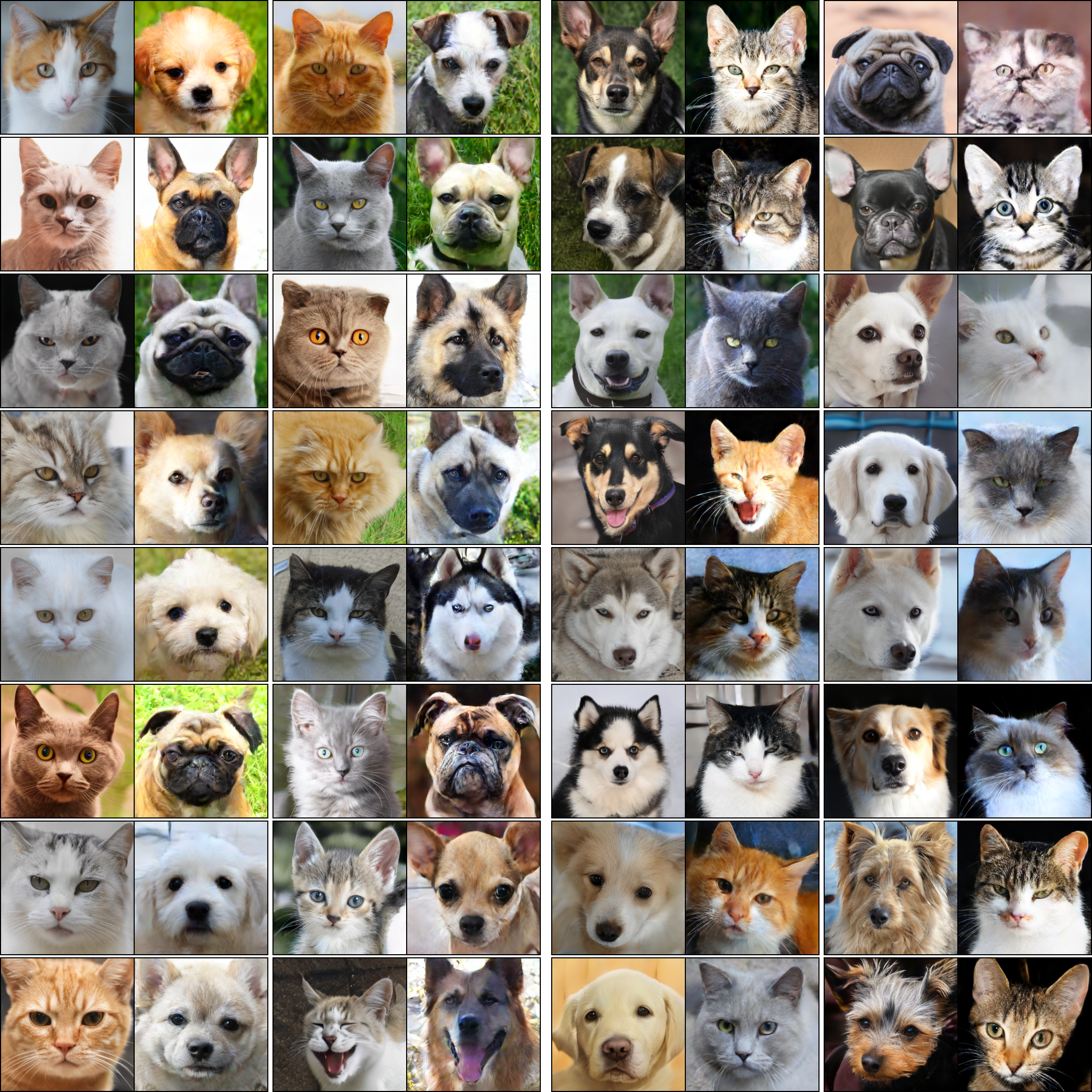
Refer to caption
Figure 11: Generation results on CelebA.
Refer to caption
Figure 12: More results at 256×256256256256\times 256 resolution on unpaired dog \leftrightarrow cat translation. Left: cat to dog; right: dog to cat. For each case, the left is the input image and the right is the translated result from our model.
Refer to caption
Figure 13: More results at 512×512512512512\times 512 resolution on unpaired dog \leftrightarrow cat translation. Left: cat to dog; right: dog to cat. For each case, the left is the input image and the right is the translated result from our model.