tcb@breakable
Calibrating Large Language Models Using Their Generations Only
Abstract
As large language models (LLMs) are increasingly deployed in user-facing applications, building trust and maintaining safety by accurately quantifying a model’s confidence in its prediction becomes even more important.
However, finding effective ways to calibrate LLMs—especially when the only interface to the models is their generated text—remains a challenge.
We propose APRICOT ![]() (Auxiliary prediction of confidence targets): A method to set confidence targets and train an additional model that predicts an LLM’s confidence based on its textual input and output alone.
This approach has several advantages: It is conceptually simple, does not require access to the target model beyond its output, does not interfere with the language generation, and has a multitude of potential usages, for instance by verbalizing the predicted confidence or adjusting the given answer based on the confidence.
We show how our approach performs competitively in terms of calibration error for white-box and black-box LLMs on closed-book question-answering to detect incorrect LLM answers.
(Auxiliary prediction of confidence targets): A method to set confidence targets and train an additional model that predicts an LLM’s confidence based on its textual input and output alone.
This approach has several advantages: It is conceptually simple, does not require access to the target model beyond its output, does not interfere with the language generation, and has a multitude of potential usages, for instance by verbalizing the predicted confidence or adjusting the given answer based on the confidence.
We show how our approach performs competitively in terms of calibration error for white-box and black-box LLMs on closed-book question-answering to detect incorrect LLM answers.
1 Introduction
When given a case description of “A man superglued his face to a piano and he says it’s making it hard to get a full night of sleep”, a recently released medical LLM was found to list unrelated potential causes in its diagnosis, including narcolepsy, sleep apnea and others.111https://x.com/spiantado/status/1620459270180569090 (last accessed Nov. 7, 2023). This, of course, ignores the seemingly obvious reason for the patient’s complaints. While humorous, this example illustrates the pitfalls of practical LLM applications: Despite often looking convincing on the surface—especially to non-experts—model responses can be wrong or unreliable, leading to potentially harmful outcomes or a loss of trust in the system, foregoing its benefits. Indeed, consistent behavior (imagine e.g. reliably indicating a lack of confidence for unsure responses) has been argued as one way to build trust in automated systems (Jacovi et al., 2021), while misleading predictions have been empirically shown to lead to a loss of trust that can be hard to recover from (Dhuliawala et al., 2023).
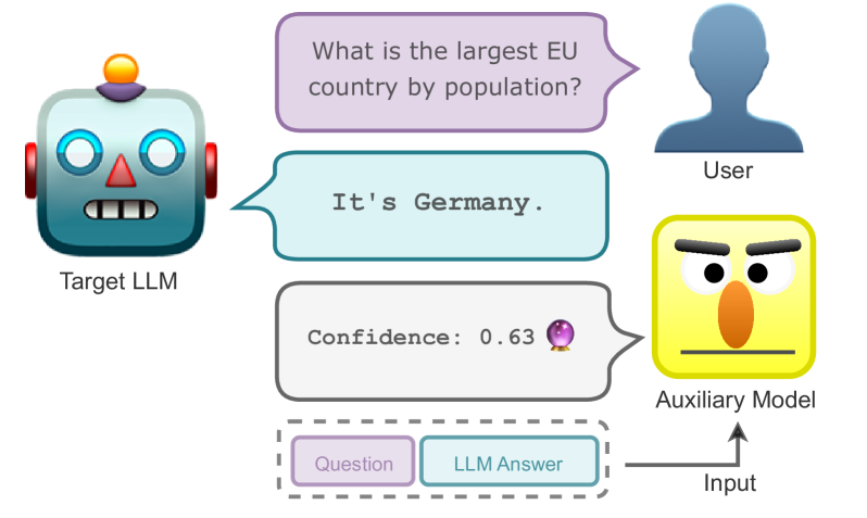
 : We train an auxiliary model to predict a target LLM’s confidence based on its input and the generated answer.
We introduce APRICOT ![]() , a method to use an auxiliary model to infer a LLM’s confidence in an open-ended question-answering setting.
The auxiliary model does so based on the given input to and generated output text from the LLM alone.
The model is trained by using these two parts as input and predicting calibration targets.
The latter are obtained without access to the LLM’s sequence likelihoods or internal states by clustering input representations produced by an additional embedding model, and thus only require black-box access.
This especially relevant since an increasing number of LLM providers safeguard their model behind black-box APIs.
This approach is conceptually straightforward, easy to optimize, and opens up a large number of possible applications, for instance, verbalizing uncertainty—a recently popular way to communicate uncertainty for LLMs (Lin et al., 2022; Xiong et al., 2023)—or adjusting a model’s response with linguistic markers of confidence.
, a method to use an auxiliary model to infer a LLM’s confidence in an open-ended question-answering setting.
The auxiliary model does so based on the given input to and generated output text from the LLM alone.
The model is trained by using these two parts as input and predicting calibration targets.
The latter are obtained without access to the LLM’s sequence likelihoods or internal states by clustering input representations produced by an additional embedding model, and thus only require black-box access.
This especially relevant since an increasing number of LLM providers safeguard their model behind black-box APIs.
This approach is conceptually straightforward, easy to optimize, and opens up a large number of possible applications, for instance, verbalizing uncertainty—a recently popular way to communicate uncertainty for LLMs (Lin et al., 2022; Xiong et al., 2023)—or adjusting a model’s response with linguistic markers of confidence.
Our contributions are as follows: We propose to obtain calibration targets without requiring any additional information about LLM internals or question metadata. We show that using auxiliary models on the target LLM’s input and output is sufficient to predict a useful notion of confidence. We also perform additional studies to identify which parts of the LLM’s output are most useful to predict confidence. All the code is openly available.222https://github.com/parameterlab/apricot.
2 Related Work
Trustworthiness in ML systems.
Trustworthiness has been identified as a key challenge to exploit the potential applications of automated systems (Marcus, 2020; Goldblum et al., 2023). This trait is seen as especially under risk in the presence of out-of-distribution examples or distributional shift (Ovadia et al., 2019; D’Amour et al., 2022). As illustrated by the introductory example, addressing these problems is paramount in high-stakes domains such as healthcare (He et al., 2019; Ulmer et al., 2020; van der Meijden et al., 2023), analyzing asylum cases (Nalbandian, 2022), or legal deliberations (Chalkidis, 2023; Dahl et al., 2024). Jacovi et al. (2021) argue that trust in automated systems can for instance be built extrinsically, e.g. through consistent and predictable behavior. One such a way is uncertainty quantification, i.e. by supplying a user with scores reflecting the reliability of a model prediction (Bhatt et al., 2021; Liao and Sundar, 2022; Hasan et al., 2023). However, the lab experiments of Dhuliawala et al. (2023) also demonstrate the flip side of this: When exposing human participants to unreliable confidence estimates, they measure a decrease in trust and participant outcomes alike. Therefore, a method like ours can help to build trust in LLMs and pave the way for reaping their benefits.
Uncertainty Quantification for LLMs.
While methods for predictive uncertainty quantification have already been explored in NLP for classification (Ulmer et al., 2022a; Van Landeghem et al., 2022; Vazhentsev et al., 2023), regression (Beck et al., 2016; Glushkova et al., 2021; Zerva et al., 2022a) and language generation tasks (Xiao et al., 2020; Malinin and Gales, 2021), their application to LLMs has posed novel challenges. Besides the different kinds of uncertainty due to the nature of language itself (Baan et al., 2023), LLMs are usually too large for Bayesian methods and are more expensive to be finetuned (unless one resorts to low-rank approximations; Yang et al., 2023). Furthermore, the generation process is often shielded behind black-box APIs for commercial models, only leaving access to the predicted probabilities, or—in the worst case—the generated text. Existing approaches operate on the model’s confidence and improve it through (re-)calibration (Tian et al., 2023; Chen et al., 2024; Bakman et al., 2024), the ensembling of prompts (Jiang et al., 2023; Hou et al., 2023), asking the model to rate its own uncertainty (Lin et al., 2022; Chen and Mueller, 2023; Tian et al., 2023) or analyzing its use of linguistic markers (Zhou et al., 2023), computing the entropy over sets of generations with similar meaning (Kuhn et al., 2023) or comparing the textual similarity of generations for the same input (Lin et al., 2023). The most similar work to ours comes from Mielke et al. (2022), who train a calibrator on the target model’s hidden states to predict whether the answer is correct or incorrect. They then finetune the target model using control tokens that are based on the calibrator’s prediction and indicate the desired confidence level. In comparison, our method has multiple advantages: We only assume access to the input question and text outputs, not requiring white-box model access or finetuning of the target model. We further demonstrate in our experiments that using more fine-grained targets than the simple binary yields better calibration overall.
Predicting properties of generated text.
Instead of trying to obtain a piece of information of interest—e.g. truthfulness or predictive confidence—from the original model, other works have investigated whether this can be done so through secondary (neural) models. For instance, Lahlou et al. (2023); Mukhoti et al. (2023) fit density estimators on internal model representations. In NLP, Pacchiardi et al. (2023) demonstrated that wrong statements by LLMs can be detected by collecting yes / no answers for a set of questions, storing them in a vector and fitting a logistic regression model. In general, using secondary neural models to predict properties of the generated text also has connections to other tasks such as translation quality estimation (Blatz et al., 2004; Quirk, 2004; Wang et al., 2019; Glushkova et al., 2021; Zerva et al., 2022b), toxicity classification (Maslej-Krešňáková et al., 2020) or fine-grained reward modeling (Wu et al., 2023).
3 Methodology
| Method | Black-box LLM? | Consistent? | Calibrated? |
|---|---|---|---|
| Seq. likelihoods | ✗ | ✔ | ✗ |
| Verb. uncertainty | ✔ | ✗ | ✗ |
| APRICOT |
✔ | ✔ | ✔ |
Estimating the confidence of a LLM can be challenging, since their size rules out many traditional techniques that require finetuning or access to model parameters.
In this light, using the likelihood of the generated sequence might seem like an appealing alternative;
however, it might not actually reflect the reliability of the model’s answer and often cannot be retrieved when using black-box models, where the only output is the generated text.
Verbalized uncertainty, i.e. prompting the LLM to express its uncertainty in words, can be a solution when the model is powerful enough.
But as we later show in Section 4, the generated confidence expressions are not very diverse, and results are not always consistent, meaning that the model does not always generate a desired confidence self-assessment.
As we illustrate in Table 1, our method, APRICOT ![]() , fulfills all of these criteria:
Through a one-time finetuning procedure of an auxiliary model on the target LLMs outputs, we have full control over a calibrated model that gives consistent and precise confidence estimates.
, fulfills all of these criteria:
Through a one-time finetuning procedure of an auxiliary model on the target LLMs outputs, we have full control over a calibrated model that gives consistent and precise confidence estimates.
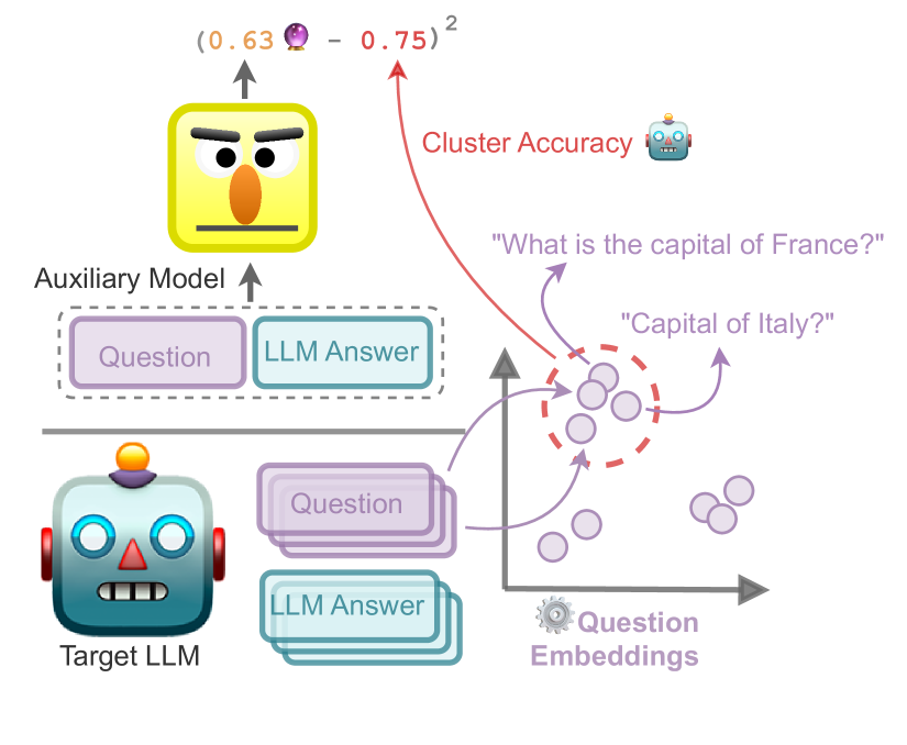
 . We collect a LLM’s answer to a set of questions and embed the latter using an embedding model. After clustering similar questions and identifying the LLM’s accuracy on them, we can use this value as reference when training to predict the confidence from a question-answer pair.
In Figure 2 we give an overview of APRICOT ![]() , which consists of three main steps:
Firstly, we prompt the target LLM to generate training data for our auxiliary model (Section 3.1).
Secondly, we set calibration targets in a way that does not require access to the target LLM beyond its generated outputs (Section 3.2).
Lastly, we train the auxiliary calibrator to predict the target LLM’s confidence for a given question (Section 3.3).
Thereby, we contribute two parts that are agnostic to the LLM in question: The creation of calibration targets and their prediction through the auxiliary model.
Note that we will use the terms auxiliary model or calibrator interchangeably in the following sections.
, which consists of three main steps:
Firstly, we prompt the target LLM to generate training data for our auxiliary model (Section 3.1).
Secondly, we set calibration targets in a way that does not require access to the target LLM beyond its generated outputs (Section 3.2).
Lastly, we train the auxiliary calibrator to predict the target LLM’s confidence for a given question (Section 3.3).
Thereby, we contribute two parts that are agnostic to the LLM in question: The creation of calibration targets and their prediction through the auxiliary model.
Note that we will use the terms auxiliary model or calibrator interchangeably in the following sections.
3.1 Prompting the Target LLM


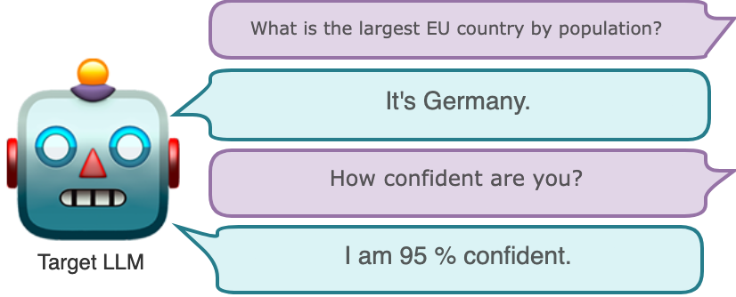
In this step, we generate finetuning data for the auxiliary model by prompting the target LLM on the given task. Here, we explore different variations to see which model response might provide the best training signal for the auxiliary calibrator. More concretely, while the original prompt and model generation might already suffice to predict the model’s confidence, we also ask the model to elaborate on its answer using chain-of-thought prompting (Wei et al., 2022). We hypothesize that including additional reasoning steps could expose signals that are useful for the calibrator.333We do this while acknowledging evidence by Turpin et al. (2023) that shows that any chain-of-thought reasoning might not reflect the actual reasons for a specific model response. We furthermore take a model’s assessment of its confidence into account, too. Recent works on verbalized uncertainty (Lin et al., 2022; Tian et al., 2023) investigated how to elicit such an assessment as a percentage value, e.g. “I am 95 % confident in my answer”, or using linguistic expressions such as “My confidence is somewhat low”. While previous studies like Zhou et al. (2024) have demonstrated the difficulty in obtaining reliable self-assessments, we can just treat them as additional input features, and let their importance be determined through the auxiliary model training. We illustrate the different prompting strategies in Figure 3 and list the exact prompts in Section A.1.
3.2 Setting Calibration Targets
After explaining the inputs to the auxiliary model, the question naturally arises about what the calibrator should be trained to predict. The work by Mielke et al. (2022) introduces an additional model that simply predicts individual answer correctness (and does so by using the target model’s internal hidden states, which is not possible for black-box models). While we also check test this type of output in Section 4.2), we show that we can produce better calibration targets through clustering.
Background.
We consider the notion of calibration by Guo et al. (2017): We define a predictor as calibrated when given some predicted outcome and some associated probability , we have
| (1) |
i.e. the probability corresponding to the actual relative frequency of correct predictions. This quantity is often approximated empirically through means such as the expected calibration error (ECE; Naeini et al., 2015). It evaluates the error
| (2) |
where in the case of the ECE, the expectation is computed by grouping test predictions into equally wide bins. Defining as the set indices that belong to bin , we can write the ECE as
| (3) |
where is the indicator function showing whether the prediction was correct. As Guo et al. (2017) note, both terms in the difference approximate the left-hand and right-hand side in Equation 1 per bin, respectively.
Contribution.
Our key insight is here that we can optimize an objective similar to Equation 2, inspired by the way that the ECE in Equation 3 aggregates samples in homogeneous groups and measures the group-wise accuracy. This done without changing the LLM’s original answers or access to token probabilities. Instead of creating bins by confidence, which is not possible in a black-box setting, we create clustered sets of inputs with similar sentence embeddings. Calibration targets are then obtained by using the observed accuracy per set . This is similar to Lin et al. (2022), who consider the accuracy per question category. Yet in the absence of such metadata, we expect good embedding and clustering algorithms to roughly group inputs by category. Höltgen and Williamson (2023) also echo a similar sentiment, describing how ECE’s grouping by confidence can be abstracted to other kinds of similarities. They also provide a proof that the calibration error of a predictor based on a -nearest neighbor clustering tends to zero in the infinite data limit.
Practically, we embed questions into a latent space using a light-weight model such as SentenceBERT (Reimers and Gurevych, 2019), normalize the embeddings along the feature dimension (Timkey and van Schijndel, 2021), and then use HDBSCAN (Campello et al., 2013) to cluster them into questions of similar topic. The use of HDBSCAN has multiple advantages: Compared to e.g. -means, we do not have to determine the numbers of clusters in advance, and since the clustering is conducted bottom-up, clusters are not constrained to a spherical shape. Furthermore, compared to its predecessor DBSCAN (Ester et al., 1996), HDBSCAN does not require one to determine the minimum distance between points for clustering manually. We evaluate this procedure in Sections 4.1 and A.4.
3.3 Training the Auxiliary Model
After determining the input and the training targets for the auxiliary model in the previous sections, we can now describe the actual training procedure that makes it predict the target LLM’s confidence. To start, we feed the questions alongside some in-context samples into our target LLM. We retain the generated answers and create a dataset that combines the question (without in-context samples) and the target model’s answers. These are used to train the auxiliary calibrator to predict the calibration targets obtained by the clustering procedure above. In our experiments, we use DeBERTaV3 (He et al., 2023), an improvement on the original DeBERTa model (He et al., 2021) using ELECTRA-style pre-training (Clark et al., 2020) and other improvements. We then finetune it using the AdamW optimizer (Loshchilov and Hutter, 2018) in combination with a cosine learning rate schedule. We minimize the following mean squared error, where is the predicted confidence, the cluster that the input question with index belongs to and an answer given by the target LLM:
| (4) |
We also explore a variant that simply predicts whether the LLM’s answer is expected to be correct or incorrect. In this case, we optimize a binary cross-entropy loss with loss weights.444The loss weights are based on scikit-learn’s implementation using the “balanced” mode, see https://scikit-learn.org/stable/modules/generated/sklearn.utils.class_weight.compute_class_weight.html. Finally, we select the final model via the best loss on the validation set. We determine the learning rate and weight decay term through Bayesian hyperparameter search (Snoek et al., 2012), picking the best configuration by validation loss. We detail search ranges and found values in Section A.3. Training hardware and the environmental impact are discussed in Section A.6.
4 Experiments
We now demonstrate how APRICOT ![]() provides a simple yet effective solution to calibrate LLMs.
Before assessing the quality of the unsupervised clustering to determine calibration targets from Section 3, we first introduce the dataset and models.
provides a simple yet effective solution to calibrate LLMs.
Before assessing the quality of the unsupervised clustering to determine calibration targets from Section 3, we first introduce the dataset and models.
Datasets.
We employ TriviaQA (Joshi et al., 2017), a common (closed-book) question-answering dataset. Open-ended question answering is an ideal testbed for natural language generation tasks, since it is comparatively easy to check whether an answer is correct or not, so calibration has an intuitive interpretation. To preprocess TriviaQA, we create a training set of 12k examples and choose another 1.5k samples as a validation and test split, respectively.555Since the original test split does not include answers, we generate the validation and test split from the original validation split. Secondly, we run experiments on CoQA (Reddy et al., 2019), a conversational question-answering dataset in which the model is quizzed about the information in a passage of text. We treat the dataset as an open-book dataset, where the model is shown the passage and then asked one of the corresponding questions at a time. We extract a subset of the dataset to match the split sizes of TriviaQA.
Models.
For our white-box model experiments, we choose a 7 billion parameter variant of the Vicuna v1.5 model (Zheng et al., 2023),666https://huggingface.co/lmsys/vicuna-7b-v1.5. an instruction-finetuned model originating from Llama 2 (Touvron et al., 2023). For the black-box model, we opt for OpenAI’s GPT-3.5 (OpenAI, 2022).777Specifically, using version gpt-3.5-turbo-0125. Despite recent API changes granting access to token probabilities,888https://x.com/OpenAIDevs/status/1735730662362189872 (last accessed on 16.01.24). creating methods for black-box confidence estimation is still relevant for multiple reasons: Token probabilities are not available for most black-box models, they might be removed again to defend against potential security issues; and they are not always a reliable proxy for confidence.
4.1 Setting Calibration Targets by Clustering
Before beginning our main experiments, we would like to verify that our proposed methodology in Section 3.2 is sound. In particular, clustering the embeddings of questions and computing the calibration confidence targets rests on the assumption that similar questions are collected in the same cluster. Ideally, we would like to check this using metadata, which however is usually not available.
Setup.
Instead, we evaluate this through different means: We first use the all-mpnet-base-v2 model from the sentence transformers package (Reimers and Gurevych, 2019) and HDBSCAN with a minimum cluster size of to cluster questions. We then analyze the textual and semantic similarity of questions in a cluster by computing the average pair-wise ROUGE-L score (semantic; Lin, 2004)999As implemented by the evaluate package, see https://huggingface.co/docs/evaluate/index. between questions and cosine similarities between question embeddings of the same cluster (semantic). Since performing this evaluation on the entire dataset is computationally expensive, we approximate the score by using pairwise comparisons per cluster, with comparisons for ROUGE-L and for cosine similarity in total, respectively. As a control for our method (clustering), we also compute values between unrelated questions that are not in the same cluster (random).
| TriviaQA | CoQA | |||
|---|---|---|---|---|
| Textual | Semantic | Textual | Semantic | |
| Random | ||||
| Clustering | ||||
Results.
We show the results of this analysis in Table 2. We observe noticeable differences between the random baseline and the similarity for the clustering scores, both on a textual and semantic level. While there is smaller difference on a textual level due to the relatively similar wording of questions, the semantic similarity based on the encoded questions is very notable. We provide deeper analyses of this part in Section A.4, showing that this method creates diverse ranges of calibration confidence targets. This suggests two things: On the one hand, our proposed methodology is able to identify fine-grained categories of questions. On the other hand, the diversity in calibration targets indicates that we detect sets of questions on which the LLM’s accuracy varies—and that this variety should be reflected. We test the ability of different methods to do exactly this next.
4.2 Calibrating White- and Black-Box Models
We are interested to see whether auxiliary models can reliably predict the target LLM’s confidence. We describe our experimental conditions below.
Evaluation metrics.
Aside from reporting the accuracy on the question answering task, we also report several calibration metrics, including the expected calibration error (ECE; Naeini et al., 2015) using bins. In order to address any distortion of results introduced by the binning procedure, we use smooth ECE (smECE; Błasiok and Nakkiran, 2023), which avoids the binning altogether by smoothing observations using a RBF kernel. We also consider Brier score (Brier, 1950), which can be interpreted as mean-squared error for probabilistic predictions. We further show how indicative the predicted confidence is for answering a question incorrectly by measuring the AUROC. The AUROC treats the problem as a binary misprediction detection task based on the confidence scores, aggregating the results over all possible decision thresholds. In each case, we report the result alongside a bootstrap estimate of the standard error (Efron and Tibshirani, 1994) estimated from samples and test for significance using the ASO test (Del Barrio et al., 2018; Dror et al., 2019; Ulmer et al., 2022b) with and a confidence level of .
Baselines.
To contextualize the auxiliary calibrator results, we consider the following baselines: We consider the raw (length-normalized) sequence likelihoods (Seq. likelihood) as well as variant using Platt scaling (Platt et al., 1999): Using the raw likelihood and the sigmoid function , we fit two additional scalars to minimize the mean squared error on the validation set to produce a calibrated likelihood while keeping all other calibrator parameters fixed. We also compare it to the recent method of verbalized uncertainty (Lin et al., 2022; Tian et al., 2023; Anonymous, 2024), where we ask the model to assess its confidence directly. We do this by asking for confidence in percent (Verbalized ) and using a seven-point scale from “very low” to “very high” and which is mapped back to numeric confidence scores (Verbalized Qual.). Where applicable, we also distinguish between baselines with and without chain-of-thought prompting (CoT; Wei et al., 2022). We detail this scale and corresponding prompts in Section A.1. For our approach, we distinguish between confidence targets obtained through the procedure in Section 3.2 (clustering) and simply predicting whether the given answer is correct or incorrect (binary).
| TriviaQA | CoQA | ||||||||||
|---|---|---|---|---|---|---|---|---|---|---|---|
| Method | Success | Brier | ECE | smECE | AUROC | Success | Brier | ECE | smECE | AUROC | |
| Vicuna v1.5 (white-box) | Seq. likelihood | - | - | ||||||||
| Seq. likelihood (CoT) | - | - | |||||||||
| Platt scaling | - | - | |||||||||
| Platt scaling (CoT) | - | - | |||||||||
| Verbalized Qual. | 0.19 | ||||||||||
| Verbalized Qual. (CoT) | 0.25 | ||||||||||
| Verbalized | 1.00 | ||||||||||
| Verbalized (CoT) | 1.00 | ||||||||||
| \cdashline2-12 | Auxiliary (binary) | - | - | ||||||||
| Auxiliary (clustering) | - | - | |||||||||
| GPT-3.5 (black-box) | Seq. likelihood | - | - | ||||||||
| Seq. likelihood (CoT) | - | - | |||||||||
| Platt scaling | - | - | |||||||||
| Platt scaling (CoT) | - | - | |||||||||
| Verbalized Qual. | 1.00 | ||||||||||
| Verbalized Qual. (CoT) | |||||||||||
| Verbalized | 1.00 | ||||||||||
| Verbalized (CoT) | 0.99 | ||||||||||
| \cdashline2-12 | Auxiliary (binary) | - | - | ||||||||
| Auxiliary (clustering) | - | - | |||||||||
Results.
Vicuna v1.5 7B achieves accuracy on TriviaQA and on CoQA, while GPT-3.5 obtains and accuracy, respectively.101010We describe the evaluation protocol in Section A.2. Since GPT-3.5 is a closed-source model, it is hard to say whether the higher accuracy scores are due to better model quality, test data leakage, or overlap in questions in the case of TriviaQA (Lewis et al., 2021).
We present the calibration results in Table 3.
APRICOT ![]() hereby achieves the highest AUROC in all settings and among the lowest Brier scores and calibration errors.
On the latter metric, verbalized confidence beats our method, but often at the cost of a higher worst-case calibration error and lower AUROC.
In addition, the qualitative verbalized uncertainty does not work reliably for the smaller Vicuna v1.5 model.
CoT prompting seems to increase the success rate of verbalized uncertainty. The additional results on GPT-3.5 suggests that this ability might also be dependent on model size.
The effect of CoT prompting on calibration, however, remains inconsistent across different baselines.
While verbalized uncertainties often perform well according to calibration error, these results have to be taken with a grain of salt:
Especially for the relatively small 7B Vicuna v1.5 model, the generations do not always contain the desired confidence expression, as visible by the low success rate.
And even when taking the generated confidence expression, their ability to distinguish potentially correct from incorrect LLM responses remains at or close to random level.
Lastly, APRICOT
hereby achieves the highest AUROC in all settings and among the lowest Brier scores and calibration errors.
On the latter metric, verbalized confidence beats our method, but often at the cost of a higher worst-case calibration error and lower AUROC.
In addition, the qualitative verbalized uncertainty does not work reliably for the smaller Vicuna v1.5 model.
CoT prompting seems to increase the success rate of verbalized uncertainty. The additional results on GPT-3.5 suggests that this ability might also be dependent on model size.
The effect of CoT prompting on calibration, however, remains inconsistent across different baselines.
While verbalized uncertainties often perform well according to calibration error, these results have to be taken with a grain of salt:
Especially for the relatively small 7B Vicuna v1.5 model, the generations do not always contain the desired confidence expression, as visible by the low success rate.
And even when taking the generated confidence expression, their ability to distinguish potentially correct from incorrect LLM responses remains at or close to random level.
Lastly, APRICOT ![]() with clustering beats the use of binary targets for Vicuna v1.5 and GPT-3.5 on both TriviaQA and CoQA.
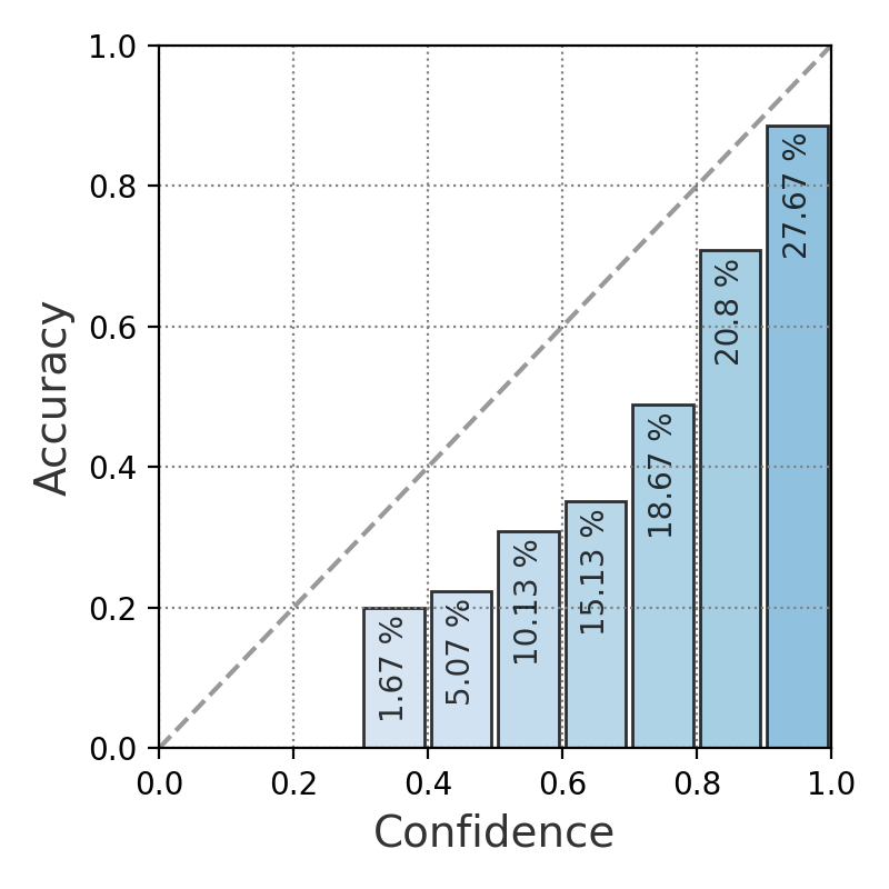
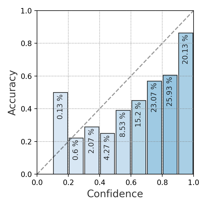
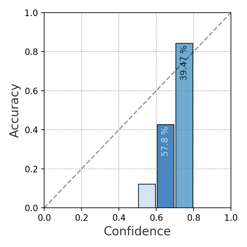
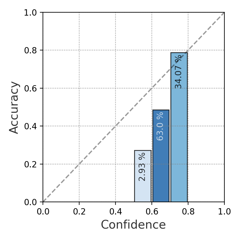
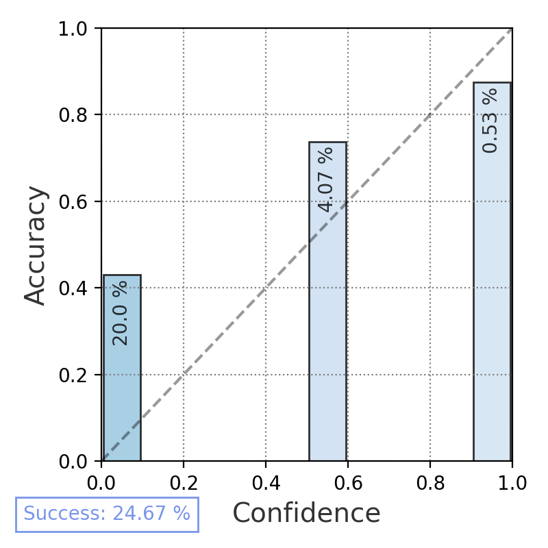
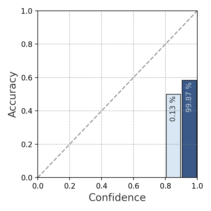
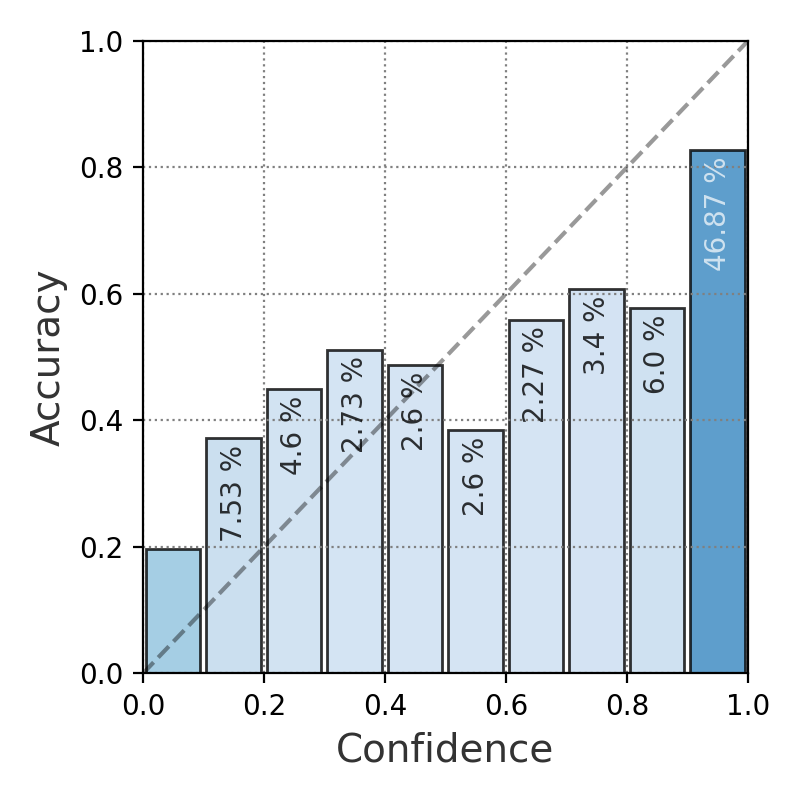
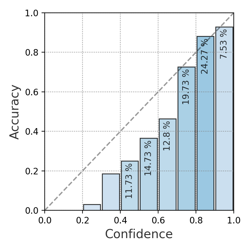
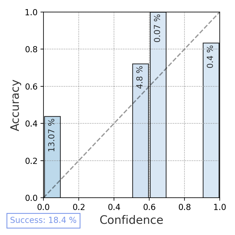
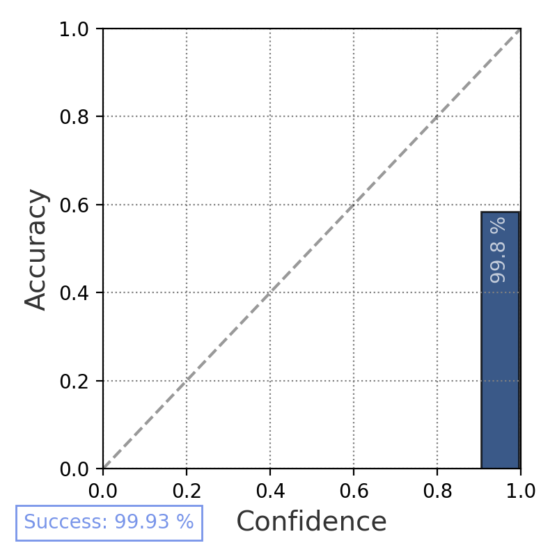
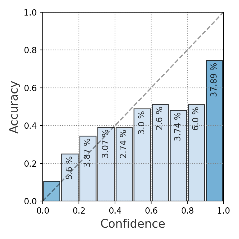
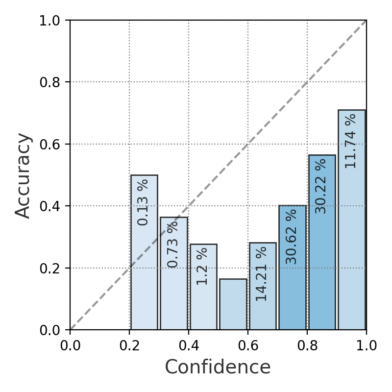
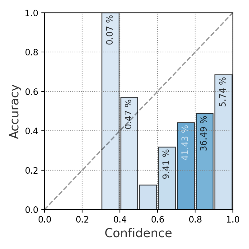
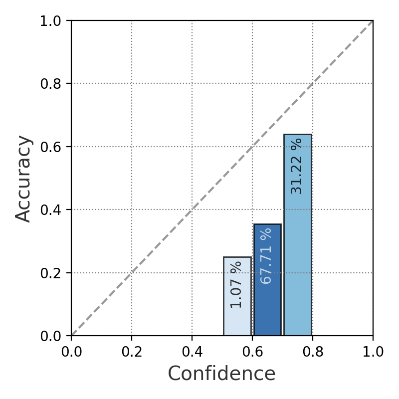
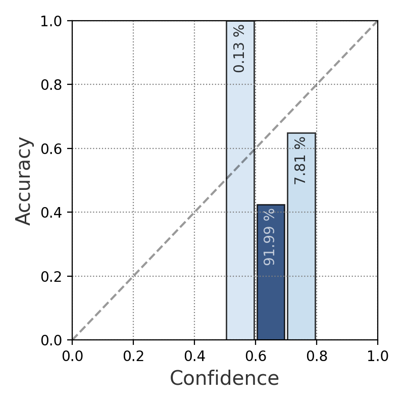
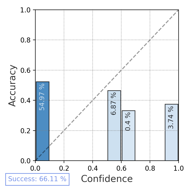
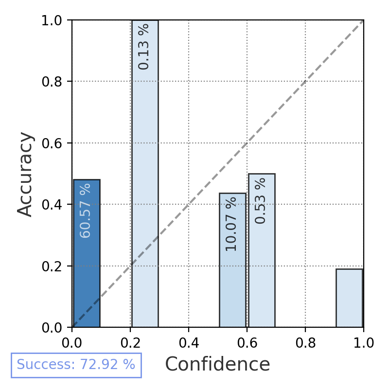
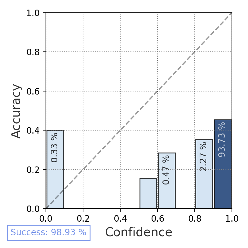
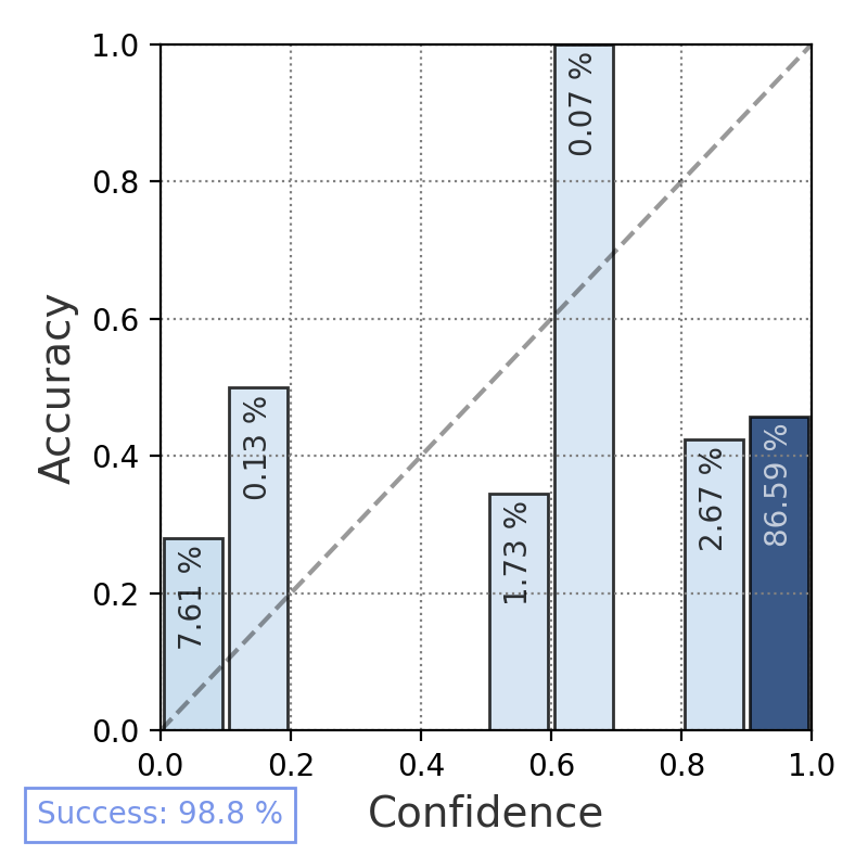
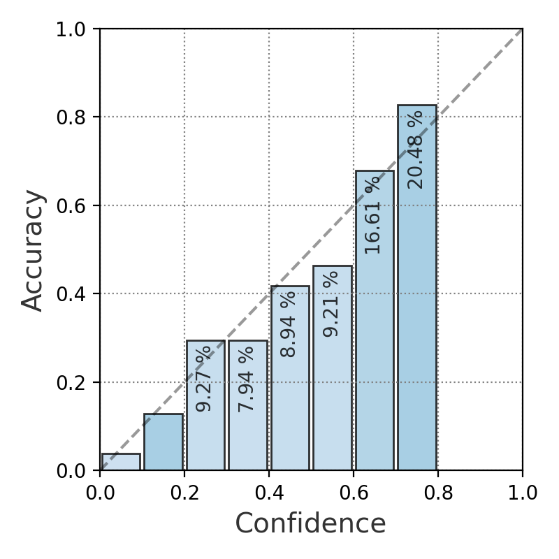
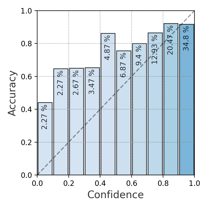
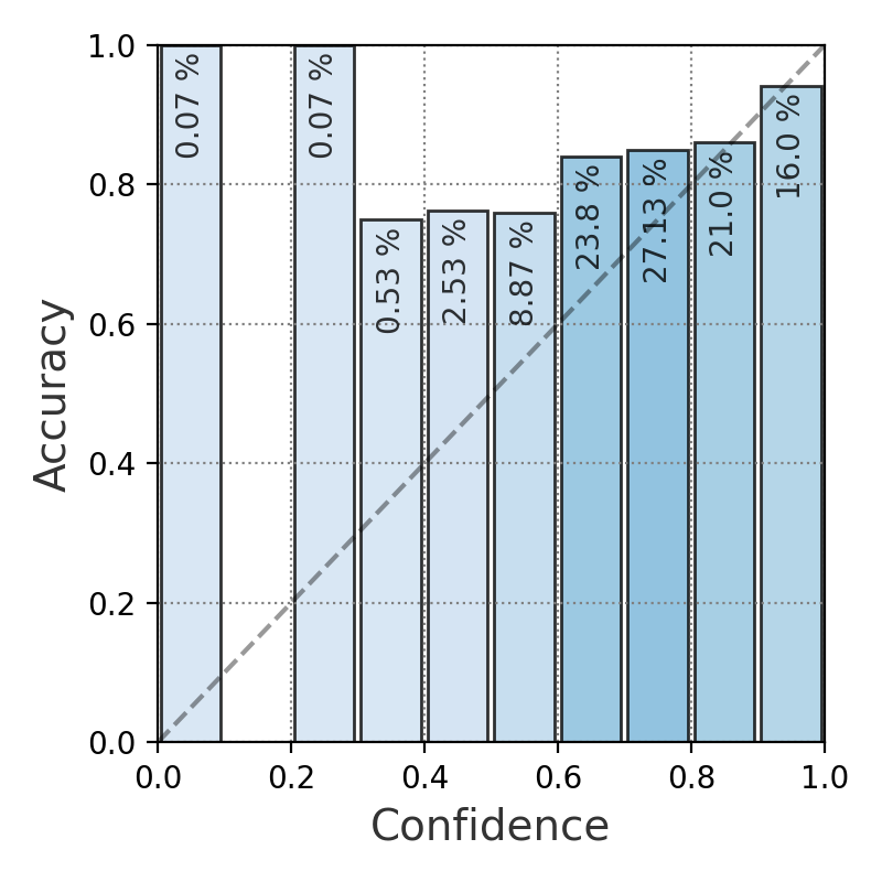
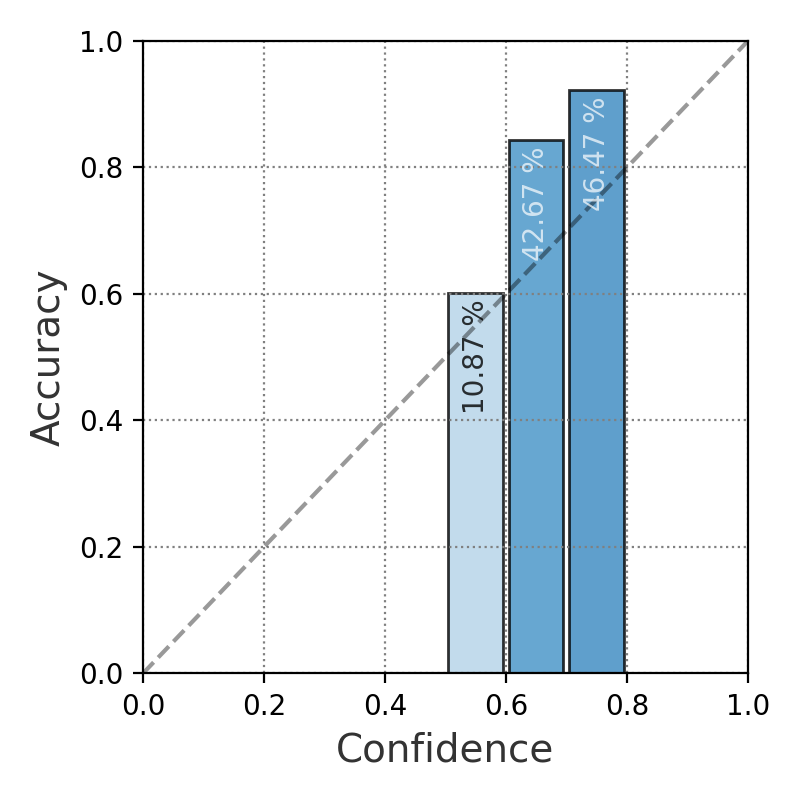
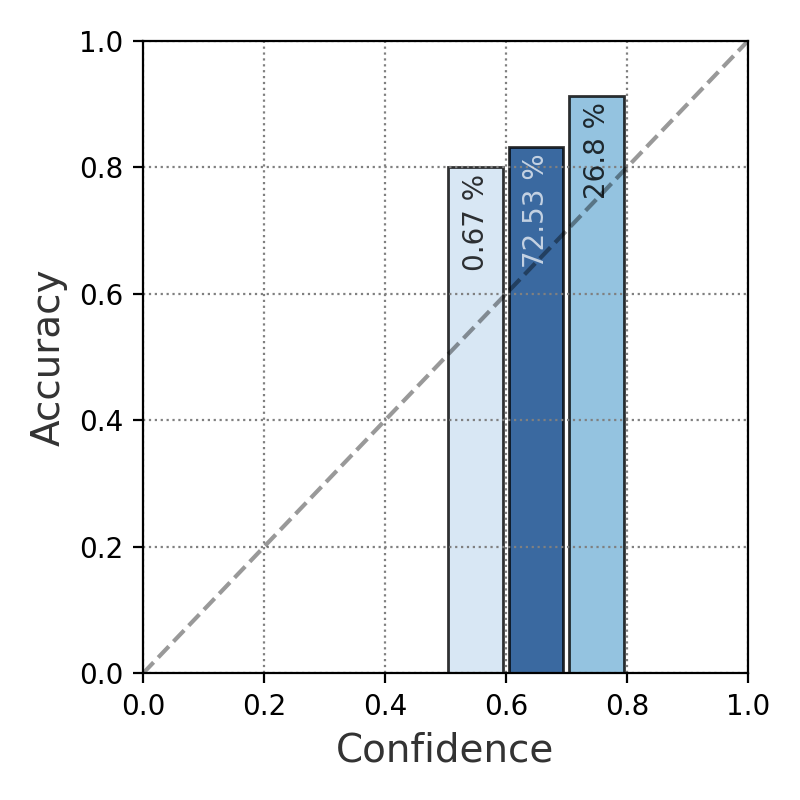
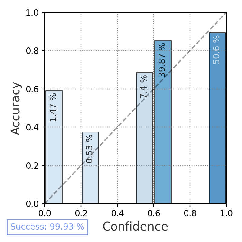
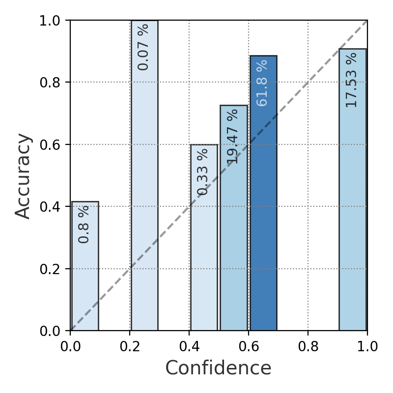
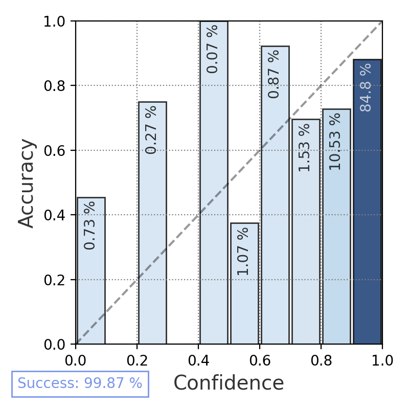
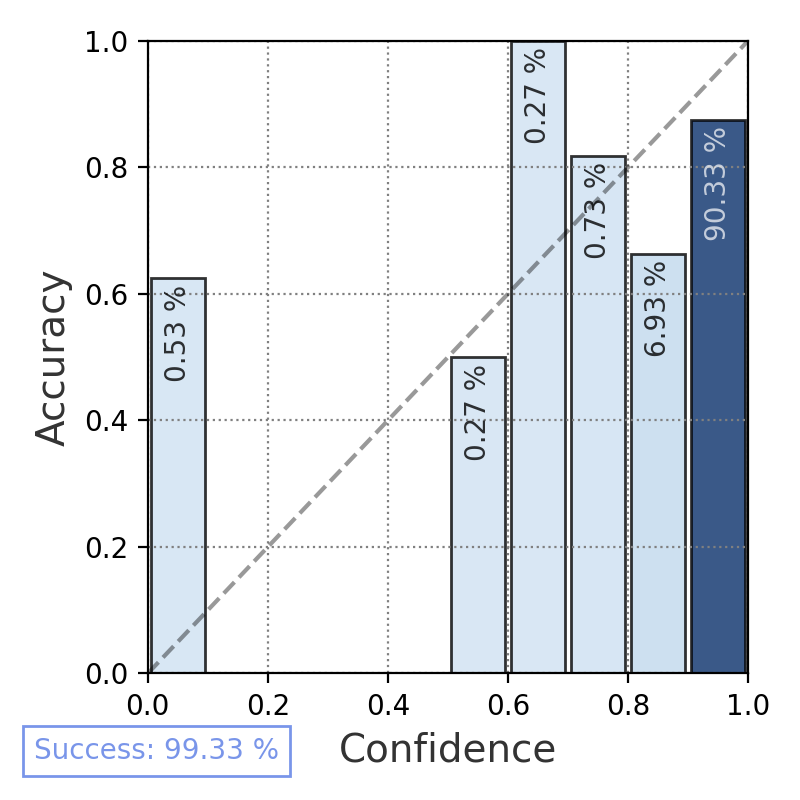
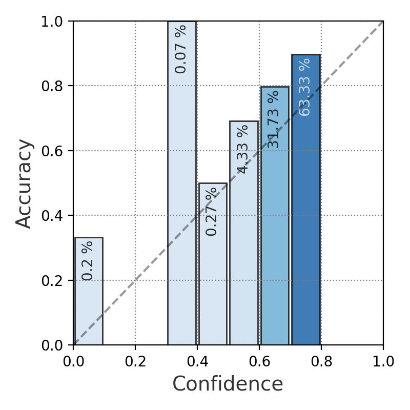
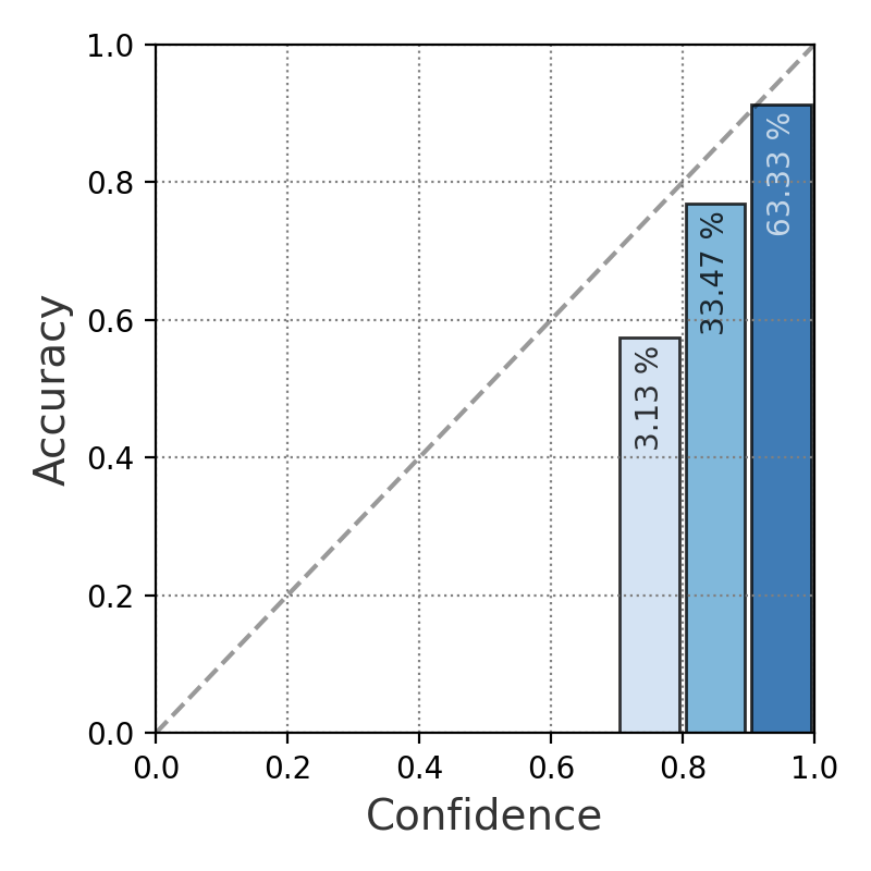
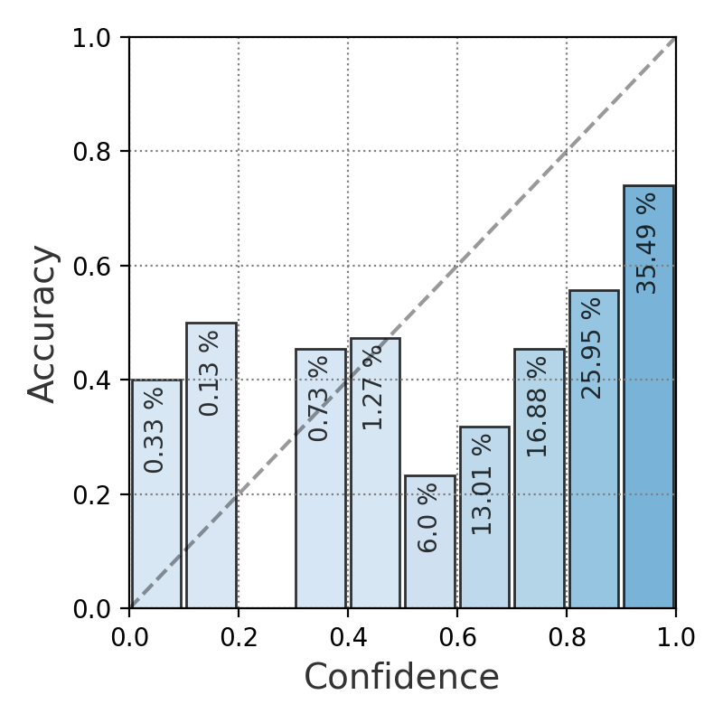
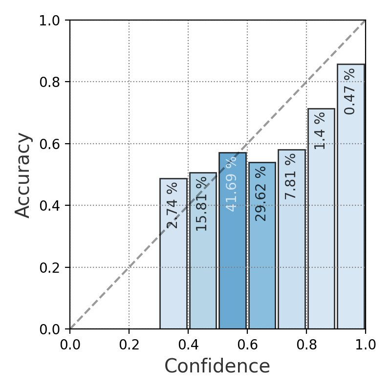
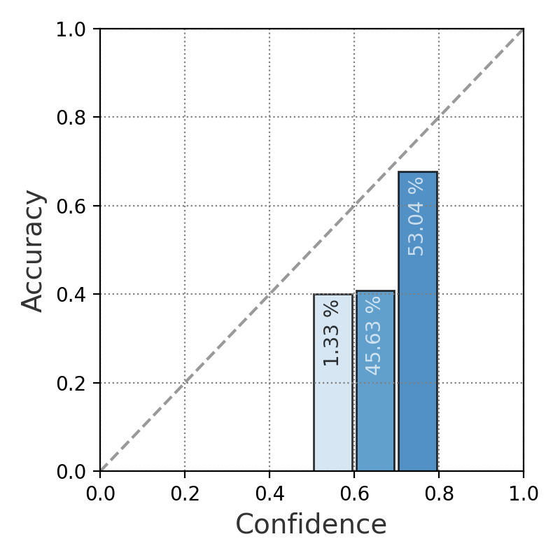
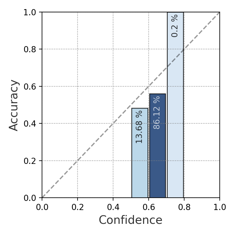
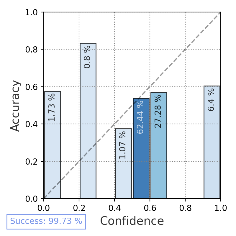
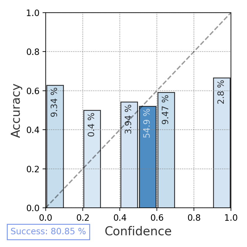
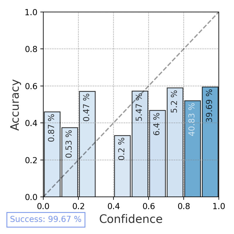
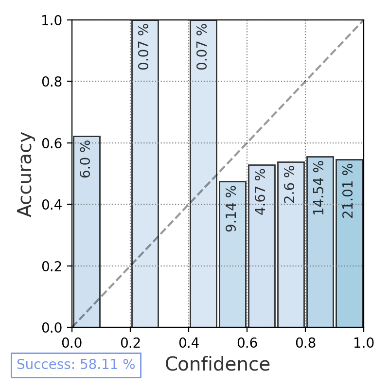
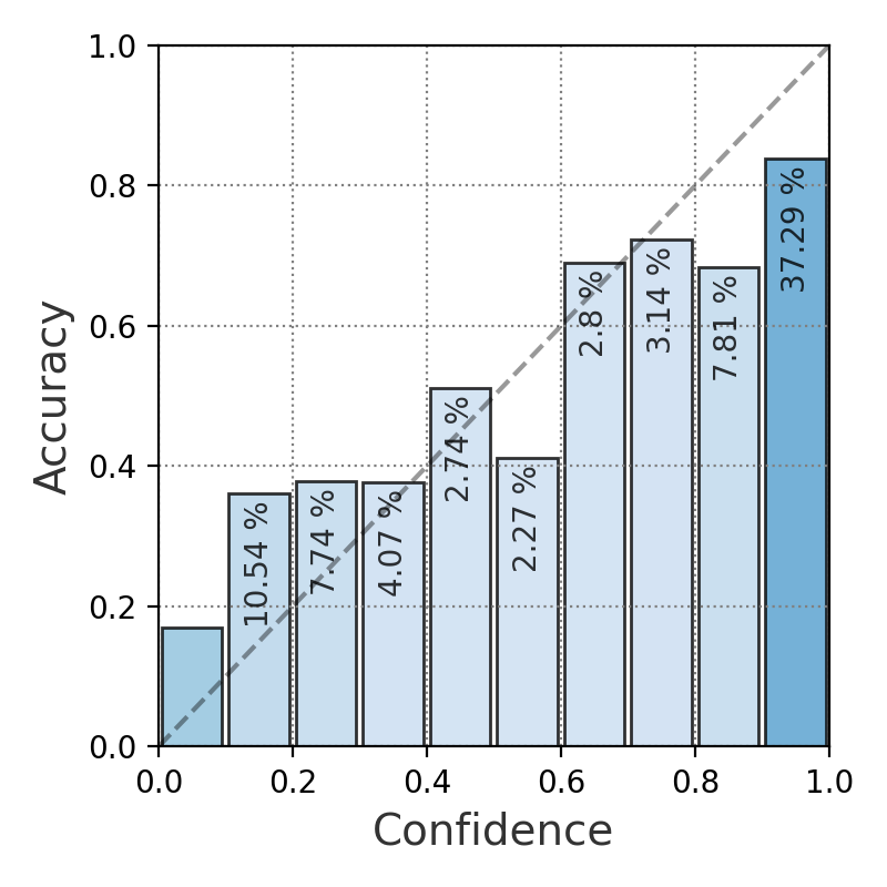
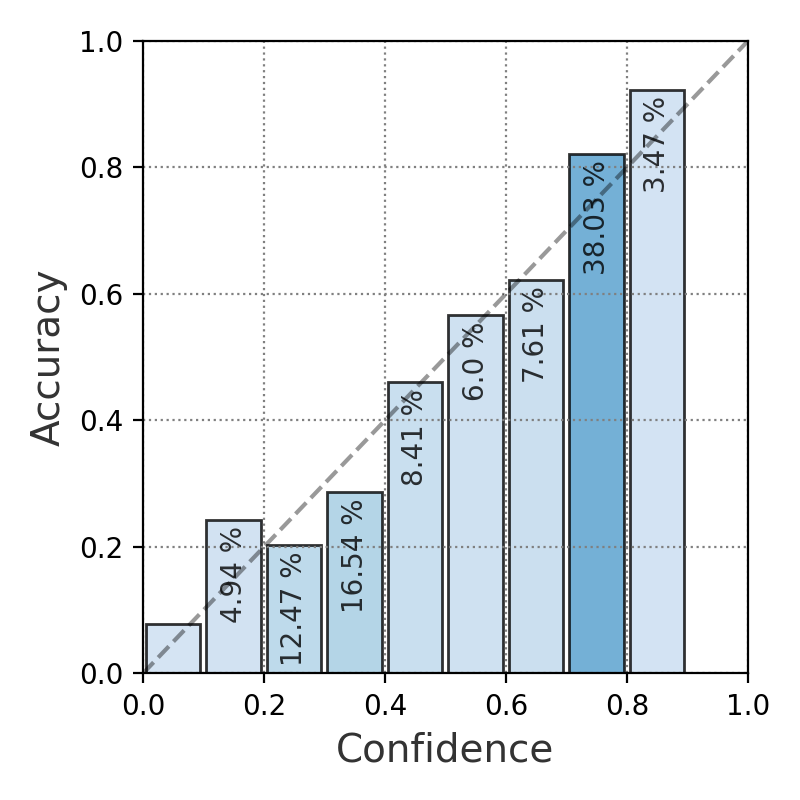
We also juxtapose reliability diagrams for the different methods for Vicuna v1.5 on TriviaQA in Figure 4 (we show the other reliability diagrams, including for GPT-3.5, in Section A.5).
Here it becomes clear that verbalized uncertainties approaches usually do not emit a wide variety of confidence scores.
This is in line with observations by Zhou et al. (2023), who hypothesize the distribution of expressions generated by verbalized uncertainty heavily depend on the mention of e.g. percentage values in the model’s training data.
While Figure 10 shows that GPT-3.5 provides more variety in this regard, the overall phenomenon persists.
We now conduct some additional analyses based on the clustering-based variant of our method.
with clustering beats the use of binary targets for Vicuna v1.5 and GPT-3.5 on both TriviaQA and CoQA.
We also juxtapose reliability diagrams for the different methods for Vicuna v1.5 on TriviaQA in Figure 4 (we show the other reliability diagrams, including for GPT-3.5, in Section A.5).
Here it becomes clear that verbalized uncertainties approaches usually do not emit a wide variety of confidence scores.
This is in line with observations by Zhou et al. (2023), who hypothesize the distribution of expressions generated by verbalized uncertainty heavily depend on the mention of e.g. percentage values in the model’s training data.
While Figure 10 shows that GPT-3.5 provides more variety in this regard, the overall phenomenon persists.
We now conduct some additional analyses based on the clustering-based variant of our method.
4.3 What does the calibrator learn from?
The previous results pose the question of which parts of input the auxiliary model actually learns from. So, analogous to the different prompting strategies in Figure 3, we explore different input variants: First, we test question-only, where the target LLM’s answer is omitted completely. We also test the performance of the calibrator when given more information, for instance the model answer with and without chain-of-thought prompting, which could potentially expose flaws in the LLM’s response.111111Based on the recent study by Turpin et al. (2023), we assume that CoT does not expose the LLM’s actual reasoning. Nevertheless, it provides more context about the given answer. Finally, we also expose the verbalized uncertainty of the LLM to the calibrator.
Results.
We show these results in Table 8 in Section A.5.
Interestingly, we can observe that even based on the question to the LLM alone, APRICOT ![]() can already achieve respectable performance across all metrics.
This suggests that the calibrator at least partially learns to infer the difficulty of the LLM answering a question from the type of question alone.
Nevertheless, we also find that adding the LLM’s actual answer further improves results, with additional gain when using CoT prompting.
In some cases, the calibration error can be improved when using the LLM’s verbalized uncertainties; in this sense, we can interpret the role of the calibrator as mapping the model’s own assessment to a calibrated confidence score.
can already achieve respectable performance across all metrics.
This suggests that the calibrator at least partially learns to infer the difficulty of the LLM answering a question from the type of question alone.
Nevertheless, we also find that adding the LLM’s actual answer further improves results, with additional gain when using CoT prompting.
In some cases, the calibration error can be improved when using the LLM’s verbalized uncertainties; in this sense, we can interpret the role of the calibrator as mapping the model’s own assessment to a calibrated confidence score.
5 Discussion
Despite the difficulty of predicting the LLM’s confidence from its generated text alone, our experiments have shown that APRICOT ![]() can be used to produce reasonable scores even under these strict constraints.
We showed in the past sections that the auxiliary model can be finetuned to learn from multiple signals.
On the one hand, the auxiliary calibrator learns a mapping from a latent category of question to the expected difficulty for a target LLM.
On the other hand, including the answer given through CoT prompting and including the LLM’s own assessment of its uncertainty helped to further improve results.
While sometimes beaten in terms of calibration error, our method consistently outperforms our baselines in misprediction AUROC, meaning that it can provide the best signal to detect wrong LLM answers.
Compared to other approaches, this yields some desirable properties:
APRICOT
can be used to produce reasonable scores even under these strict constraints.
We showed in the past sections that the auxiliary model can be finetuned to learn from multiple signals.
On the one hand, the auxiliary calibrator learns a mapping from a latent category of question to the expected difficulty for a target LLM.
On the other hand, including the answer given through CoT prompting and including the LLM’s own assessment of its uncertainty helped to further improve results.
While sometimes beaten in terms of calibration error, our method consistently outperforms our baselines in misprediction AUROC, meaning that it can provide the best signal to detect wrong LLM answers.
Compared to other approaches, this yields some desirable properties:
APRICOT ![]() is available when sequence likelihood is not; it is more reliable than verbalized uncertainty; and it only needs a light finetuning once, adding negligible inference overhead.
Compared to other methods such as Kuhn et al. (2023); Lin et al. (2023), it also does not require more generations for the same input, reducing the more expensive LLM inference costs.
is available when sequence likelihood is not; it is more reliable than verbalized uncertainty; and it only needs a light finetuning once, adding negligible inference overhead.
Compared to other methods such as Kuhn et al. (2023); Lin et al. (2023), it also does not require more generations for the same input, reducing the more expensive LLM inference costs.
6 Conclusion
We presented APRICOT ![]() , a general method to obtain confidence scores from any language model on the input and text output alone.
We showed that it is possible to compute calibration targets through the clustering of question embeddings.
Through the subsequent finetuning of a smaller language model, we then outperform other methods to distinguish incorrect from correct answers with competitive calibration scores, on different models and datasets.
While we only presented a first, more fundamental version this approach in this work, it lends itself naturally to a whole body of research that aims to improve the calibration of pretrained language models (Desai and Durrett, 2020; Jiang et al., 2021; Chen et al., 2023).
Lastly, future studies might also investigate the uncertainty of the auxiliary model itself and use techniques such as conformal prediction (Vovk et al., 2005; Papadopoulos et al., 2002; Angelopoulos and Bates, 2021) to produce estimates of LLM confidence intervals.
, a general method to obtain confidence scores from any language model on the input and text output alone.
We showed that it is possible to compute calibration targets through the clustering of question embeddings.
Through the subsequent finetuning of a smaller language model, we then outperform other methods to distinguish incorrect from correct answers with competitive calibration scores, on different models and datasets.
While we only presented a first, more fundamental version this approach in this work, it lends itself naturally to a whole body of research that aims to improve the calibration of pretrained language models (Desai and Durrett, 2020; Jiang et al., 2021; Chen et al., 2023).
Lastly, future studies might also investigate the uncertainty of the auxiliary model itself and use techniques such as conformal prediction (Vovk et al., 2005; Papadopoulos et al., 2002; Angelopoulos and Bates, 2021) to produce estimates of LLM confidence intervals.
Limitations
Clustering.
While yielding generally positive results in our case, the clustering methodology from Section 3.2 requires access to a sufficiently expressive sentence embedding model and a large enough number of data points. When this is not given, we show that the binary approach—tuning the auxiliary model to predict misprediction—is a viable alternative that can even outperform the clustering variant in some settings.
Distributional shift.
As any neural model, the auxiliary calibrator might be prone to distributional shift and out-of-distribution data. Further research could help to understand how this issue can be reduced and which parts of the input the model identifies to predict confidence scores in order to unveil potential shortcut learning (Du et al., 2023).
Other types of language generation.
Our experiments focused on open-ended question answering tasks, which provide an easy way to check answer correctness. In other types of language generation such as summarization, translation or open text generation, this notion is not given. However, we point out the relation of our approach to other NLP tasks in Section 2, which might provide an opening for future research.
Ethical Considerations
We mostly see any ethical considerations with our work arising in the general nature of neural models, which therefore also affects our auxiliary calibrator. The efficacy of neural models might vary on out-of-distribution data. In safety-sensitive applications, this also means that its predictions might be less trustworthy on certain sub-populations. In this case, explicit validation of the LLM’s answers and the auxiliary calibrators corresponding predictions is necessary and further finetuning might be necessary. In these cases, reporting the confidence score alongside an answer might also be replaced by withholding the LLM’s response, entirely.
Acknowledgements
This work was generously supported by the NAVER corporation.
References
- Angelopoulos and Bates (2021) Anastasios N Angelopoulos and Stephen Bates. 2021. A gentle introduction to conformal prediction and distribution-free uncertainty quantification. arXiv preprint arXiv:2107.07511.
- Anonymous (2024) Anonymous. 2024. Can LLMs express their uncertainty? an empirical evaluation of confidence elicitation in LLMs. In The Twelfth International Conference on Learning Representations.
- Baan et al. (2023) Joris Baan, Nico Daheim, Evgenia Ilia, Dennis Ulmer, Haau-Sing Li, Raquel Fernández, Barbara Plank, Rico Sennrich, Chrysoula Zerva, and Wilker Aziz. 2023. Uncertainty in natural language generation: From theory to applications. arXiv preprint arXiv:2307.15703.
- Bakman et al. (2024) Yavuz Faruk Bakman, Duygu Nur Yaldiz, Baturalp Buyukates, Chenyang Tao, Dimitrios Dimitriadis, and Salman Avestimehr. 2024. Mars: Meaning-aware response scoring for uncertainty estimation in generative llms. arXiv preprint arXiv:2402.11756.
- Beck et al. (2016) Daniel Beck, Lucia Specia, and Trevor Cohn. 2016. Exploring prediction uncertainty in machine translation quality estimation. In Proceedings of the 20th SIGNLL Conference on Computational Natural Language Learning, pages 208–218, Berlin, Germany. Association for Computational Linguistics.
- Bhatt et al. (2021) Umang Bhatt, Javier Antorán, Yunfeng Zhang, Q Vera Liao, Prasanna Sattigeri, Riccardo Fogliato, Gabrielle Melançon, Ranganath Krishnan, Jason Stanley, Omesh Tickoo, et al. 2021. Uncertainty as a form of transparency: Measuring, communicating, and using uncertainty. In Proceedings of the 2021 AAAI/ACM Conference on AI, Ethics, and Society, pages 401–413.
- Biewald (2020) Lukas Biewald. 2020. Experiment tracking with weights and biases. Software available from wandb.com.
- Błasiok and Nakkiran (2023) Jarosław Błasiok and Preetum Nakkiran. 2023. Smooth ece: Principled reliability diagrams via kernel smoothing. arXiv preprint arXiv:2309.12236.
- Blatz et al. (2004) John Blatz, Erin Fitzgerald, George Foster, Simona Gandrabur, Cyril Goutte, Alex Kulesza, Alberto Sanchis, and Nicola Ueffing. 2004. Confidence estimation for machine translation. In Coling 2004: Proceedings of the 20th international conference on computational linguistics, pages 315–321.
- Brier (1950) Glenn W Brier. 1950. Verification of forecasts expressed in terms of probability. Monthly weather review, 78(1):1–3.
- Campello et al. (2013) Ricardo JGB Campello, Davoud Moulavi, and Jörg Sander. 2013. Density-based clustering based on hierarchical density estimates. In Pacific-Asia conference on knowledge discovery and data mining, pages 160–172. Springer.
- Chalkidis (2023) Ilias Chalkidis. 2023. Chatgpt may pass the bar exam soon, but has a long way to go for the lexglue benchmark. arXiv preprint arXiv:2304.12202.
- Chen and Mueller (2023) Jiuhai Chen and Jonas Mueller. 2023. Quantifying uncertainty in answers from any language model via intrinsic and extrinsic confidence assessment. arXiv preprint arXiv:2308.16175.
- Chen et al. (2024) Lihu Chen, Alexandre Perez-Lebel, Fabian M Suchanek, and Gaël Varoquaux. 2024. Reconfidencing llms from the grouping loss perspective. arXiv preprint arXiv:2402.04957.
- Chen et al. (2023) Yangyi Chen, Lifan Yuan, Ganqu Cui, Zhiyuan Liu, and Heng Ji. 2023. A close look into the calibration of pre-trained language models. In Proceedings of the 61st Annual Meeting of the Association for Computational Linguistics (Volume 1: Long Papers), ACL 2023, Toronto, Canada, July 9-14, 2023, pages 1343–1367. Association for Computational Linguistics.
- Clark et al. (2020) Kevin Clark, Minh-Thang Luong, Quoc V. Le, and Christopher D. Manning. 2020. ELECTRA: pre-training text encoders as discriminators rather than generators. In 8th International Conference on Learning Representations, ICLR 2020, Addis Ababa, Ethiopia, April 26-30, 2020. OpenReview.net.
- Dahl et al. (2024) Matthew Dahl, Varun Magesh, Mirac Suzgun, and Daniel E Ho. 2024. Large legal fictions: Profiling legal hallucinations in large language models. arXiv preprint arXiv:2401.01301.
- D’Amour et al. (2022) Alexander D’Amour, Katherine Heller, Dan Moldovan, Ben Adlam, Babak Alipanahi, Alex Beutel, Christina Chen, Jonathan Deaton, Jacob Eisenstein, Matthew D Hoffman, et al. 2022. Underspecification presents challenges for credibility in modern machine learning. The Journal of Machine Learning Research, 23(1):10237–10297.
- Del Barrio et al. (2018) Eustasio Del Barrio, Juan A Cuesta-Albertos, and Carlos Matrán. 2018. An optimal transportation approach for assessing almost stochastic order. In The Mathematics of the Uncertain, pages 33–44. Springer.
- Desai and Durrett (2020) Shrey Desai and Greg Durrett. 2020. Calibration of pre-trained transformers. In Proceedings of the 2020 Conference on Empirical Methods in Natural Language Processing, EMNLP 2020, Online, November 16-20, 2020, pages 295–302. Association for Computational Linguistics.
- Dhuliawala et al. (2023) Shehzaad Dhuliawala, Vilém Zouhar, Mennatallah El-Assady, and Mrinmaya Sachan. 2023. A diachronic perspective on user trust in ai under uncertainty. arXiv preprint arXiv:2310.13544.
- Dror et al. (2019) Rotem Dror, Segev Shlomov, and Roi Reichart. 2019. Deep dominance - how to properly compare deep neural models. In Proceedings of the 57th Conference of the Association for Computational Linguistics, ACL 2019, Florence, Italy, July 28- August 2, 2019, Volume 1: Long Papers, pages 2773–2785. Association for Computational Linguistics.
- Du et al. (2023) Mengnan Du, Fengxiang He, Na Zou, Dacheng Tao, and Xia Hu. 2023. Shortcut learning of large language models in natural language understanding. Communications of the ACM, 67(1):110–120.
- Efron and Tibshirani (1994) Bradley Efron and Robert J Tibshirani. 1994. An introduction to the bootstrap. CRC press.
- Ester et al. (1996) Martin Ester, Hans-Peter Kriegel, Jörg Sander, and Xiaowei Xu. 1996. A density-based algorithm for discovering clusters in large spatial databases with noise. In Proceedings of the Second International Conference on Knowledge Discovery and Data Mining (KDD-96), Portland, Oregon, USA, pages 226–231. AAAI Press.
- Glushkova et al. (2021) Taisiya Glushkova, Chrysoula Zerva, Ricardo Rei, and André F. T. Martins. 2021. Uncertainty-aware machine translation evaluation. In Findings of the Association for Computational Linguistics: EMNLP 2021, pages 3920–3938, Punta Cana, Dominican Republic. Association for Computational Linguistics.
- Goldblum et al. (2023) Micah Goldblum, Anima Anandkumar, Richard Baraniuk, Tom Goldstein, Kyunghyun Cho, Zachary C Lipton, Melanie Mitchell, Preetum Nakkiran, Max Welling, and Andrew Gordon Wilson. 2023. Perspectives on the state and future of deep learning–2023. arXiv preprint arXiv:2312.09323.
- Guo et al. (2017) Chuan Guo, Geoff Pleiss, Yu Sun, and Kilian Q Weinberger. 2017. On calibration of modern neural networks. In International conference on machine learning, pages 1321–1330. PMLR.
- Hasan et al. (2023) Mehedi Hasan, Moloud Abdar, Abbas Khosravi, Uwe Aickelin, Pietro Lio, Ibrahim Hossain, Ashikur Rahman, and Saeid Nahavandi. 2023. Survey on leveraging uncertainty estimation towards trustworthy deep neural networks: The case of reject option and post-training processing. arXiv preprint arXiv:2304.04906.
- He et al. (2019) Jianxing He, Sally L Baxter, Jie Xu, Jiming Xu, Xingtao Zhou, and Kang Zhang. 2019. The practical implementation of artificial intelligence technologies in medicine. Nature medicine, 25(1):30–36.
- He et al. (2023) Pengcheng He, Jianfeng Gao, and Weizhu Chen. 2023. Debertav3: Improving deberta using electra-style pre-training with gradient-disentangled embedding sharing. In The Eleventh International Conference on Learning Representations, ICLR 2023, Kigali, Rwanda, May 1-5, 2023. OpenReview.net.
- He et al. (2021) Pengcheng He, Xiaodong Liu, Jianfeng Gao, and Weizhu Chen. 2021. Deberta: decoding-enhanced bert with disentangled attention. In 9th International Conference on Learning Representations, ICLR 2021, Virtual Event, Austria, May 3-7, 2021. OpenReview.net.
- Höltgen and Williamson (2023) Benedikt Höltgen and Robert C Williamson. 2023. On the richness of calibration. In Proceedings of the 2023 ACM Conference on Fairness, Accountability, and Transparency, pages 1124–1138.
- Hou et al. (2023) Bairu Hou, Yujian Liu, Kaizhi Qian, Jacob Andreas, Shiyu Chang, and Yang Zhang. 2023. Decomposing uncertainty for large language models through input clarification ensembling. arXiv preprint arXiv:2311.08718.
- Jacovi et al. (2021) Alon Jacovi, Ana Marasović, Tim Miller, and Yoav Goldberg. 2021. Formalizing trust in artificial intelligence: Prerequisites, causes and goals of human trust in ai. In Proceedings of the 2021 ACM conference on fairness, accountability, and transparency, pages 624–635.
- Jiang et al. (2023) Mingjian Jiang, Yangjun Ruan, Sicong Huang, Saifei Liao, Silviu Pitis, Roger Baker Grosse, and Jimmy Ba. 2023. Calibrating language models via augmented prompt ensembles.
- Jiang et al. (2021) Zhengbao Jiang, Jun Araki, Haibo Ding, and Graham Neubig. 2021. How can we know When language models know? on the calibration of language models for question answering. Trans. Assoc. Comput. Linguistics, 9:962–977.
- Joshi et al. (2017) Mandar Joshi, Eunsol Choi, Daniel S. Weld, and Luke Zettlemoyer. 2017. Triviaqa: A large scale distantly supervised challenge dataset for reading comprehension. In Proceedings of the 55th Annual Meeting of the Association for Computational Linguistics, ACL 2017, Vancouver, Canada, July 30 - August 4, Volume 1: Long Papers, pages 1601–1611. Association for Computational Linguistics.
- Kuhn et al. (2023) Lorenz Kuhn, Yarin Gal, and Sebastian Farquhar. 2023. Semantic uncertainty: Linguistic invariances for uncertainty estimation in natural language generation. In The Eleventh International Conference on Learning Representations, ICLR 2023, Kigali, Rwanda, May 1-5, 2023. OpenReview.net.
- Lacoste et al. (2019) Alexandre Lacoste, Alexandra Luccioni, Victor Schmidt, and Thomas Dandres. 2019. Quantifying the carbon emissions of machine learning. Workshop on Tackling Climate Change with Machine Learning at NeurIPS 2019.
- Lahlou et al. (2023) Salem Lahlou, Moksh Jain, Hadi Nekoei, Victor Butoi, Paul Bertin, Jarrid Rector-Brooks, Maksym Korablyov, and Yoshua Bengio. 2023. DEUP: direct epistemic uncertainty prediction. Trans. Mach. Learn. Res., 2023.
- Lewis et al. (2021) Patrick S. H. Lewis, Pontus Stenetorp, and Sebastian Riedel. 2021. Question and answer test-train overlap in open-domain question answering datasets. In Proceedings of the 16th Conference of the European Chapter of the Association for Computational Linguistics: Main Volume, EACL 2021, Online, April 19 - 23, 2021, pages 1000–1008. Association for Computational Linguistics.
- Liao and Sundar (2022) Q Vera Liao and S Shyam Sundar. 2022. Designing for responsible trust in ai systems: A communication perspective. In Proceedings of the 2022 ACM Conference on Fairness, Accountability, and Transparency, pages 1257–1268.
- Lin (2004) Chin-Yew Lin. 2004. Rouge: A package for automatic evaluation of summaries. In Text summarization branches out, pages 74–81.
- Lin et al. (2022) Stephanie Lin, Jacob Hilton, and Owain Evans. 2022. Teaching models to express their uncertainty in words. Trans. Mach. Learn. Res., 2022.
- Lin et al. (2023) Zhen Lin, Shubhendu Trivedi, and Jimeng Sun. 2023. Generating with confidence: Uncertainty quantification for black-box large language models. arXiv preprint arXiv:2305.19187.
- Loshchilov and Hutter (2018) Ilya Loshchilov and Frank Hutter. 2018. Fixing weight decay regularization in adam.
- Lottick et al. (2019) Kadan Lottick, Silvia Susai, Sorelle A. Friedler, and Jonathan P. Wilson. 2019. Energy usage reports: Environmental awareness as part of algorithmic accountability. Workshop on Tackling Climate Change with Machine Learning at NeurIPS 2019.
- Malinin and Gales (2021) Andrey Malinin and Mark J. F. Gales. 2021. Uncertainty estimation in autoregressive structured prediction. In 9th International Conference on Learning Representations, ICLR 2021, Virtual Event, Austria, May 3-7, 2021. OpenReview.net.
- Marcus (2020) Gary Marcus. 2020. The next decade in ai: four steps towards robust artificial intelligence. arXiv preprint arXiv:2002.06177.
- Maslej-Krešňáková et al. (2020) Viera Maslej-Krešňáková, Martin Sarnovskỳ, Peter Butka, and Kristína Machová. 2020. Comparison of deep learning models and various text pre-processing techniques for the toxic comments classification. Applied Sciences, 10(23):8631.
- Mielke et al. (2022) Sabrina J Mielke, Arthur Szlam, Emily Dinan, and Y-Lan Boureau. 2022. Reducing conversational agents’ overconfidence through linguistic calibration. Transactions of the Association for Computational Linguistics, 10:857–872.
- Mukhoti et al. (2023) Jishnu Mukhoti, Andreas Kirsch, Joost van Amersfoort, Philip HS Torr, and Yarin Gal. 2023. Deep deterministic uncertainty: A new simple baseline. In Proceedings of the IEEE/CVF Conference on Computer Vision and Pattern Recognition, pages 24384–24394.
- Naeini et al. (2015) Mahdi Pakdaman Naeini, Gregory Cooper, and Milos Hauskrecht. 2015. Obtaining well calibrated probabilities using bayesian binning. In Proceedings of the AAAI conference on artificial intelligence, volume 29.
- Nalbandian (2022) Lucia Nalbandian. 2022. An eye for an ‘i:’a critical assessment of artificial intelligence tools in migration and asylum management. Comparative Migration Studies, 10(1):1–23.
- OpenAI (2022) OpenAI. 2022. Introducing chatgpt.
- Ovadia et al. (2019) Yaniv Ovadia, Emily Fertig, Jie Ren, Zachary Nado, David Sculley, Sebastian Nowozin, Joshua Dillon, Balaji Lakshminarayanan, and Jasper Snoek. 2019. Can you trust your model’s uncertainty? evaluating predictive uncertainty under dataset shift. Advances in neural information processing systems, 32.
- Pacchiardi et al. (2023) Lorenzo Pacchiardi, Alex J Chan, Sören Mindermann, Ilan Moscovitz, Alexa Y Pan, Yarin Gal, Owain Evans, and Jan Brauner. 2023. How to catch an ai liar: Lie detection in black-box llms by asking unrelated questions. arXiv preprint arXiv:2309.15840.
- Papadopoulos et al. (2002) Harris Papadopoulos, Kostas Proedrou, Volodya Vovk, and Alex Gammerman. 2002. Inductive confidence machines for regression. In Machine Learning: ECML 2002: 13th European Conference on Machine Learning Helsinki, Finland, August 19–23, 2002 Proceedings 13, pages 345–356. Springer.
- Platt et al. (1999) John Platt et al. 1999. Probabilistic outputs for support vector machines and comparisons to regularized likelihood methods. Advances in large margin classifiers, 10(3):61–74.
- Quirk (2004) Christopher Quirk. 2004. Training a sentence-level machine translation confidence measure. In LREC.
- Reddy et al. (2019) Siva Reddy, Danqi Chen, and Christopher D Manning. 2019. Coqa: A conversational question answering challenge. Transactions of the Association for Computational Linguistics, 7:249–266.
- Reimers and Gurevych (2019) Nils Reimers and Iryna Gurevych. 2019. Sentence-bert: Sentence embeddings using siamese bert-networks. In Proceedings of the 2019 Conference on Empirical Methods in Natural Language Processing and the 9th International Joint Conference on Natural Language Processing, EMNLP-IJCNLP 2019, Hong Kong, China, November 3-7, 2019, pages 3980–3990. Association for Computational Linguistics.
- Schmidt et al. (2021) Victor Schmidt, Kamal Goyal, Aditya Joshi, Boris Feld, Liam Conell, Nikolas Laskaris, Doug Blank, Jonathan Wilson, Sorelle Friedler, and Sasha Luccioni. 2021. CodeCarbon: Estimate and Track Carbon Emissions from Machine Learning Computing.
- Snoek et al. (2012) Jasper Snoek, Hugo Larochelle, and Ryan P Adams. 2012. Practical bayesian optimization of machine learning algorithms. Advances in neural information processing systems, 25.
- Tian et al. (2023) Katherine Tian, Eric Mitchell, Allan Zhou, Archit Sharma, Rafael Rafailov, Huaxiu Yao, Chelsea Finn, and Christopher D. Manning. 2023. Just ask for calibration: Strategies for eliciting calibrated confidence scores from language models fine-tuned with human feedback. In Proceedings of the 2023 Conference on Empirical Methods in Natural Language Processing, EMNLP 2023, Singapore, December 6-10, 2023, pages 5433–5442. Association for Computational Linguistics.
- Timkey and van Schijndel (2021) William Timkey and Marten van Schijndel. 2021. All bark and no bite: Rogue dimensions in transformer language models obscure representational quality. In Proceedings of the 2021 Conference on Empirical Methods in Natural Language Processing, EMNLP 2021, Virtual Event / Punta Cana, Dominican Republic, 7-11 November, 2021, pages 4527–4546. Association for Computational Linguistics.
- Touvron et al. (2023) Hugo Touvron, Louis Martin, Kevin Stone, Peter Albert, Amjad Almahairi, Yasmine Babaei, Nikolay Bashlykov, Soumya Batra, Prajjwal Bhargava, Shruti Bhosale, et al. 2023. Llama 2: Open foundation and fine-tuned chat models. arXiv preprint arXiv:2307.09288.
- Turpin et al. (2023) Miles Turpin, Julian Michael, Ethan Perez, and Samuel R Bowman. 2023. Language models don’t always say what they think: Unfaithful explanations in chain-of-thought prompting. arXiv preprint arXiv:2305.04388.
- Ulmer et al. (2022a) Dennis Ulmer, Jes Frellsen, and Christian Hardmeier. 2022a. Exploring predictive uncertainty and calibration in NLP: A study on the impact of method & data scarcity. In Findings of the Association for Computational Linguistics: EMNLP 2022, Abu Dhabi, United Arab Emirates, December 7-11, 2022, pages 2707–2735. Association for Computational Linguistics.
- Ulmer et al. (2022b) Dennis Ulmer, Christian Hardmeier, and Jes Frellsen. 2022b. deep-significance: Easy and meaningful signifcance testing in the age of neural networks. In ML Evaluation Standards Workshop at the Tenth International Conference on Learning Representations.
- Ulmer et al. (2020) Dennis Ulmer, Lotta Meijerink, and Giovanni Cinà. 2020. Trust issues: Uncertainty estimation does not enable reliable ood detection on medical tabular data. In Machine Learning for Health, pages 341–354. PMLR.
- van der Meijden et al. (2023) Siri L van der Meijden, Anne AH de Hond, Patrick J Thoral, Ewout W Steyerberg, Ilse MJ Kant, Giovanni Cinà, and M Sesmu Arbous. 2023. Intensive care unit physicians’ perspectives on artificial intelligence–based clinical decision support tools: Preimplementation survey study. JMIR Human Factors, 10:e39114.
- Van Landeghem et al. (2022) Jordy Van Landeghem, Matthew Blaschko, Bertrand Anckaert, and Marie-Francine Moens. 2022. Benchmarking scalable predictive uncertainty in text classification. IEEE Access.
- Vazhentsev et al. (2023) Artem Vazhentsev, Gleb Kuzmin, Akim Tsvigun, Alexander Panchenko, Maxim Panov, Mikhail Burtsev, and Artem Shelmanov. 2023. Hybrid uncertainty quantification for selective text classification in ambiguous tasks. In Proceedings of the 61st Annual Meeting of the Association for Computational Linguistics (Volume 1: Long Papers), ACL 2023, Toronto, Canada, July 9-14, 2023, pages 11659–11681. Association for Computational Linguistics.
- Vovk et al. (2005) Vladimir Vovk, Alexander Gammerman, and Glenn Shafer. 2005. Algorithmic learning in a random world, volume 29. Springer.
- Wang et al. (2019) Shuo Wang, Yang Liu, Chao Wang, Huanbo Luan, and Maosong Sun. 2019. Improving back-translation with uncertainty-based confidence estimation. In Proceedings of the 2019 Conference on Empirical Methods in Natural Language Processing and the 9th International Joint Conference on Natural Language Processing, EMNLP-IJCNLP 2019, Hong Kong, China, November 3-7, 2019, pages 791–802. Association for Computational Linguistics.
- Wang et al. (2021) Yingfan Wang, Haiyang Huang, Cynthia Rudin, and Yaron Shaposhnik. 2021. Understanding how dimension reduction tools work: an empirical approach to deciphering t-sne, umap, trimap, and pacmap for data visualization. The Journal of Machine Learning Research, 22(1):9129–9201.
- Wei et al. (2022) Jason Wei, Xuezhi Wang, Dale Schuurmans, Maarten Bosma, Fei Xia, Ed Chi, Quoc V Le, Denny Zhou, et al. 2022. Chain-of-thought prompting elicits reasoning in large language models. Advances in Neural Information Processing Systems, 35:24824–24837.
- Wu et al. (2023) Zeqiu Wu, Yushi Hu, Weijia Shi, Nouha Dziri, Alane Suhr, Prithviraj Ammanabrolu, Noah A. Smith, Mari Ostendorf, and Hannaneh Hajishirzi. 2023. Fine-grained human feedback gives better rewards for language model training. In Thirty-seventh Conference on Neural Information Processing Systems.
- Xiao et al. (2020) Tim Z Xiao, Aidan N Gomez, and Yarin Gal. 2020. Wat zei je? detecting out-of-distribution translations with variational transformers. arXiv preprint arXiv:2006.08344.
- Xiong et al. (2023) Miao Xiong, Zhiyuan Hu, Xinyang Lu, Yifei Li, Jie Fu, Junxian He, and Bryan Hooi. 2023. Can llms express their uncertainty? an empirical evaluation of confidence elicitation in llms. CoRR, abs/2306.13063.
- Yang et al. (2023) Adam X Yang, Maxime Robeyns, Xi Wang, and Laurence Aitchison. 2023. Bayesian low-rank adaptation for large language models. arXiv preprint arXiv:2308.13111.
- Zerva et al. (2022a) Chrysoula Zerva, Taisiya Glushkova, Ricardo Rei, and André F. T. Martins. 2022a. Disentangling uncertainty in machine translation evaluation. In Proceedings of the 2022 Conference on Empirical Methods in Natural Language Processing, EMNLP 2022, Abu Dhabi, United Arab Emirates, December 7-11, 2022, pages 8622–8641. Association for Computational Linguistics.
- Zerva et al. (2022b) Chrysoula Zerva, Taisiya Glushkova, Ricardo Rei, and André FT Martins. 2022b. Better uncertainty quantification for machine translation evaluation. arXiv e-prints, pages arXiv–2204.
- Zheng et al. (2023) Lianmin Zheng, Wei-Lin Chiang, Ying Sheng, Siyuan Zhuang, Zhanghao Wu, Yonghao Zhuang, Zi Lin, Zhuohan Li, Dacheng Li, Eric Xing, et al. 2023. Judging llm-as-a-judge with mt-bench and chatbot arena. arXiv preprint arXiv:2306.05685.
- Zhou et al. (2024) Kaitlyn Zhou, Jena D Hwang, Xiang Ren, and Maarten Sap. 2024. Relying on the unreliable: The impact of language models’ reluctance to express uncertainty. arXiv preprint arXiv:2401.06730.
- Zhou et al. (2023) Kaitlyn Zhou, Dan Jurafsky, and Tatsunori Hashimoto. 2023. Navigating the grey area: Expressions of overconfidence and uncertainty in language models. arXiv preprint arXiv:2302.13439.
Appendix A Appendix
This appendix is structured as follows: We list all used prompts in Section A.1, briefly explore the evaluation protocal for the QA task in Section A.2 and list hyperparameter search details for replicability in Section A.3. The rest of the appendix is dedicated to additional results, namely for the analysis of the clustering step in Section A.4 or for the calibration experiments in Section A.5. We also list our compute hardware and its environmental impact in Section A.6.
A.1 Prompting Setup
In the following we elaborate on the prompts used in this work. In general, we use a very simple prompt for question answering, where we fill in a template of the form “Question: {Question} Answer:”. For in-context samples, we prepend the demonstrations to the input, using the sample template as above. In the case of chain-of-thought prompting, we use the prompting below:
In the case of CoQA, we slightly adjust the prompt template to the following:
Note that here the passage that questions are based on is given first, and chain-of-thought prompting is signaled through the “Instruction” field. When no chain-of-thought prompting is used, this field is omitted. For the verbalized uncertainty, we use the following prompts, in which case we omit any in-context samples:
| Expression | Value |
|---|---|
| Very low | |
| Low | |
| Somewhat low | |
| Medium | |
| Somewhat high | |
| High | |
| Very high |
When mapping these expressions back to probabilities using the mapping in Table 4.
We follow Kuhn et al. (2023) and use in-context samples for the original answer, which are randomly sampled from the training set (but in contrast to Kuhn et al., we sample different examples for each instance). When prompting for verbalized uncertainty, we remove these in-context samples.
A.2 Question-Answering Evaluation Protocol
In order to check model answers automatically, we take inspiration from the evaluation protocol by Kuhn et al. (2023). They use ROUGE-L (Lin, 2004) to compare the LLM’s answer against the reference answer, and consider the answer as correct if the resulting score surpasses . We improve this protocol by adding the following condition: If the gold answer can be found verbatim in the generated answer, the answer is also considered correct.
A.3 Finetuning Hyperparameters
We conduct suites of hyperparameter searches per target LLM, dataset and type of calibration targets (binary and clustering) corresponding to the results in Table 3, resulting in eight different suites. We then use these found hyperparameters for the results in Table 8.
| TriviaQA | CoQA | ||||
|---|---|---|---|---|---|
| Binary | Clustering | Binary | Clustering | ||
| Vicuna v1.5 | learning rate | ||||
| weight decay | |||||
| GPT-3.5 | learning rate | ||||
| weight decay | |||||
Search method and ranges.
For the search, we opt for Bayesian hyperparameter search (Snoek et al., 2012) as implemented by Weights & Biases (Biewald, 2020). We optimize only two hyperparameters: Learning rate and weight decay. The learning rate is samples from a log-uniform distribution and weight decay from a uniform distribution for a total of runs and training steps each. The final hyperparameters selected are given in Table 5.
Other hyperparameters.
When obtaining the responses from Vicuna v1.5 7B, we use a batch size of and generate for a maximum of tokens and stop generation when the model tries to generate parts of the prompt, such as “Question:” / “Q:” or “Answer:” / “A:”. We also use in-context samples for TriviaQA, but no in-context samples for CoQA. For the auxiliary calibrator, we use a context size of tokens, batch size of , gradient clipping with a maximum norm of .
A.4 Additional Clustering Results
| Cluster 1120 |
|---|
| How many fluid ounces are in one quarter of an imperial pint? |
| How many fluid ounces in one Imperial pint? |
| How many fluid ounces in half an Imperial pint? |
| Cluster 920 |
| Which famous US outlaw shot the cashier of a savings bank in Gallatin Missouri in 1869? |
| What famous outlaw committed the Wild West’s first train robbery on July 21, 1873 in Adair, Iowa? |
| On July 21, 1873, Jesse James and the James-Younger gang pulled off the first successful what of the American West, in Adair Iowa? |
| Cluster 984 |
| In what country was the game of golf invented? |
| Which ball game was invented by Dr James Naismith in Massachusetts USA in 1891? |
| It is generally accepted that the game of golf originated in what country? |
| What’s a country where most people love playing rugby? |
| What’s a country where most people love playing golf? |
| Cluster 64 |
| Which alternative word for the Devil is a Hebrew word with translates as Lord Of The Flies? |
| Beelzebub is Hebrew for what phrase, which is also the title of a famous novel? |
| Diablo is another name for who? |
| Cluster 811 |
| How many colors are there in the spectrum when white light is separated? |
| Which part of the eye contains about 137 million light-sensitive cells in one square inch? |
| Which of the retina’s cells can distinguish between different wavelengths of light? |
| In four colour process printing, which is also known as CMYK, which are the only four colours that are used? |
| How many colours are in the rainbow? |
| In art, what are the three primary colours? |
| What color consists of the longest wavelengths of lights visible by the human eye? |
| What are the three primary colours of light? |
| Cluster 74 |
| What was the name of the computer in the movie 2001: A Space Odyssey? |
| What was the name of the computer in Blake’s Seven? |
| Developed by IBM, Deep Blue was a computer that played what? |
| What was the name of the PDA produced by Apple, most famous for its handwriting recognition software turning Random House into Condom Nose during a major presentation? |
| Cluster 823 |
|---|
| Where in Europe is it located? |
| Is it in the European Plain? |
| Which region of Europe is it in? |
| Cluster 1176 |
| Did she have children? |
| Does she have any children? |
| Did she have any children? |
| Did she have any other children? |
| Cluster 2244 |
| Who won the Kentucky Derby? |
| as he won the Derby before? |
| Has he raced in the Derby before? |
| What were the winning horse’s odds? |
| How many Derbys have their been? |
| Cluster 11 |
| Are they densities of everything the same? |
| What is the densest elements at regular conditions? |
| What is density of a substance? |
| What is another symbol for density? |
| Who gives weight per unit volume as the definition? |
| Where is density the same value as it’s mass concentration? |
| To make comparisons easier what stands in for density? |
| What is the relative density of something that floats? |
| Cluster 1081 |
| Who was murdered? |
| who was killed? |
| Who committed this murder? |
| who was killed? |
| Who was killed? |
| who was killed? |
| Cluster 579 |
| Did it succeed? |
| DId they continue to try? |
| did they succeed? |
| Was it successful? |
| Did they expect that success? |
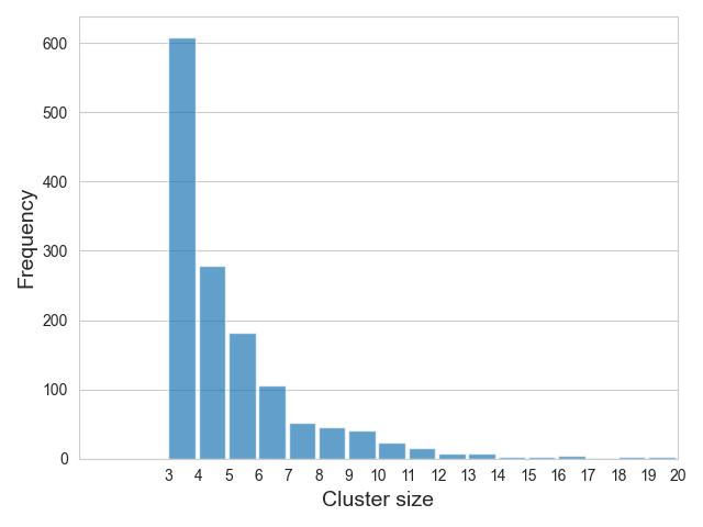
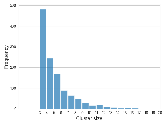
In this section we take a closer look at the results of the clustering procedure described in Section 3.2. In our experiments, we run HDBSCAN using a minimum cluster size of three, since preliminary experiments showed this number to produce the best trade-off between the coherence of cluster contents (as evaluated in Table 2) and a diversity in cluster targets. This setting yields a distribution of cluster sizes shown in Figure 5. We can see that the majority of cluster sizes are rather small, including questions on specific topics, some of which we display in Tables 6 and 7. Not shown are cluster sizes over since the distribution quickly levels off, as well the set of all points that could not be sorted into any cluster.
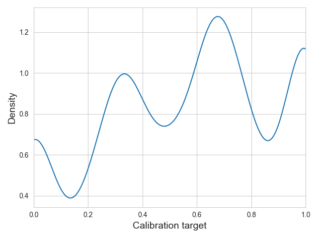
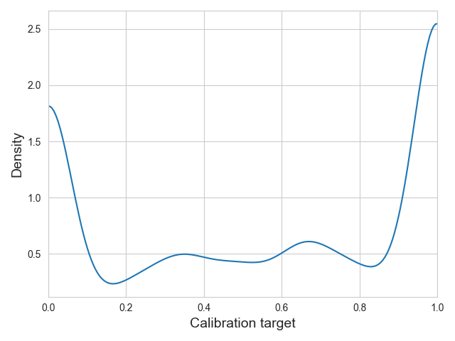
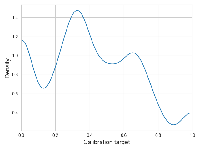
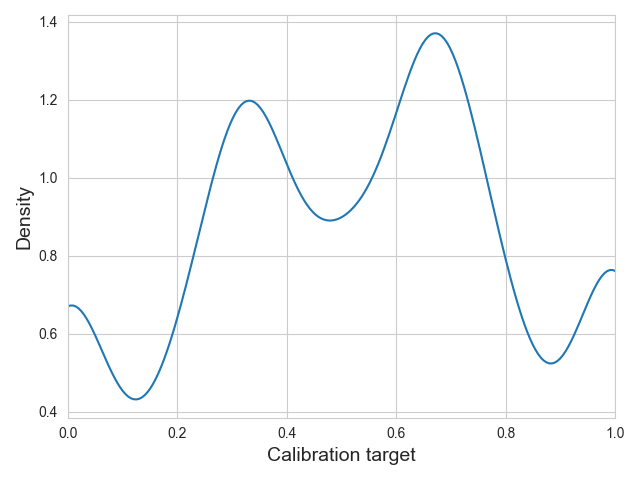
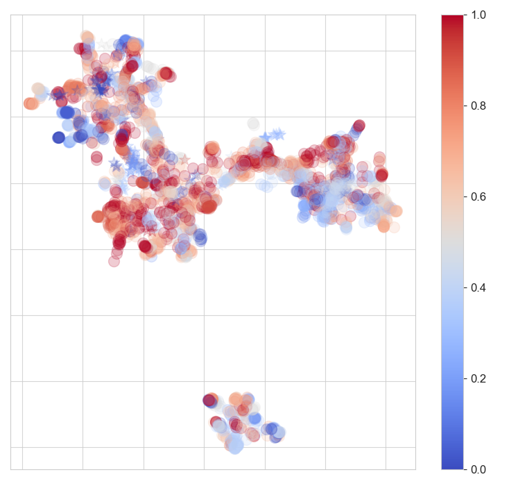
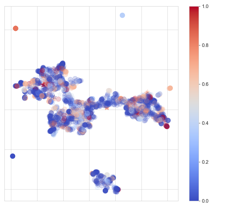
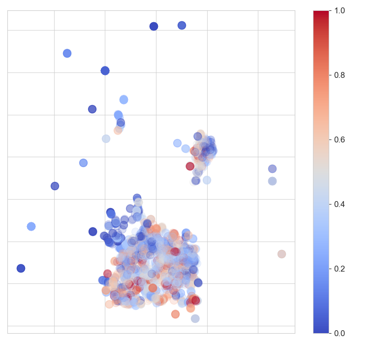
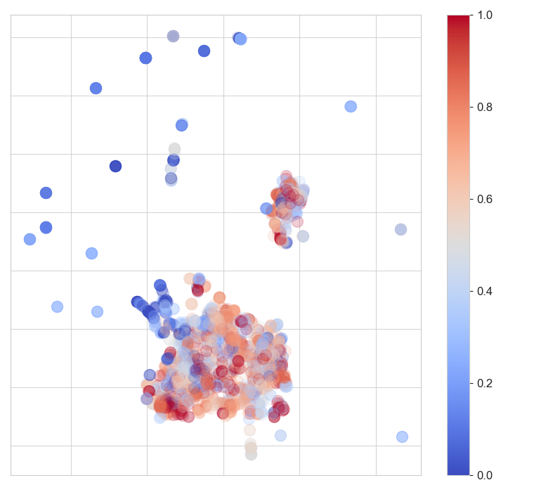
After clustering and computing the average accuracy per cluster, we obtain a distribution over calibration targets, which we show with density plots in Figure 6. Since most clusters are of size three, we can see clear modes around and for Vicuna v1.5 in Figure 6(a). For GPT-3.5 in Figure 6(b) these are however less pronounced: We see that targets are often concentrated on or , respectively. Similar spikes like in Figure 6(a) are observable for both models on CoQA in Figures 6(c) and 6(d). This trend is also visible when plotting the assigned calibration targets per datapoint in Figure 7: While we can spot more transitionary colors between the blue and red extremes in the manifold for Figure 7(a), the colors tend more to either of the options Figure 7(b). These mode trends continue for CoQA in Figure 7(c) and Figure 7(d).
A.5 Additional Calibration Results






Additional reliability plots.
We show the all available reliability diagrams for Vicuna-v1.5 for TriviaQA in Figure 4 and CoQA in Figure 9, as well as the corresponding plots for GPT-3.5 in Figures 10 and 11. We can summarize some general trends: Sequence likelihood can be well-calibrated already, but this fact depends strongly on the dataset in question. And while our version of Platt scaling can improve results, it also narrows the range of confidence values to a narrow window. Verbalized uncertainty in both of variants also is not able to produce a wide variety of responses, even though this effect is slightly less pronounced for GPT-3.5. This could be explained by previous observations by Zhou et al. (2023) that certain mentions of percentage values are over-represented in model training data. The auxiliary model is able to predict a wider array of confidence values in all settings, with the clustering variant achieving better calibration overall.
| Auxiliary Model Input | TriviaQA | CoQA | ||||||||||
|---|---|---|---|---|---|---|---|---|---|---|---|---|
| Quest. | Ans. | CoT | Verb. | Brier | ECE | smECE | AUROC | Brier | ECE | smECE | AUROC | |
| Vicuna v1.5 (white-box) | ✔ | ✗ | ✗ | ✗ | ||||||||
| ✔ | ✔ | ✗ | ✗ | |||||||||
| ✔ | ✔ | ✗ | Qual. | |||||||||
| ✔ | ✔ | ✗ | ||||||||||
| ✔ | ✔ | ✔ | ✗ | |||||||||
| ✔ | ✔ | ✔ | Qual. | |||||||||
| ✔ | ✔ | ✔ | ||||||||||
| GPT-3.5 (black-box) | ✔ | ✗ | ✗ | ✗ | ||||||||
| ✔ | ✔ | ✗ | ✗ | |||||||||
| ✔ | ✔ | ✗ | Qual. | |||||||||
| ✔ | ✔ | ✗ | ||||||||||
| ✔ | ✔ | ✔ | ✗ | |||||||||
| ✔ | ✔ | ✔ | Qual. | |||||||||
| ✔ | ✔ | ✔ | ||||||||||
Ablation results.
We show the results of the different ablations in Table 8. For both LLMs, we can see that the auxiliary model is able to achieve already decent scores by using the question as input alone. This suggest that the calibrator is learning about the general difficulty of questions for the LLM. However, both cases also show that including more information—the LLM’s answer, CoT reasoning or verbalized uncertainties—can help to improve the auxiliaries model calibration and misprediction AUROC even further, even though the effect remains somewhat inconsistent across models.
A.6 Environmental Impact
All experiments are run on a single V100 NVIDIA GPU. Using codecarbon (Schmidt et al., 2021; Lacoste et al., 2019; Lottick et al., 2019), we estimate finetuning the auxiliary calibrator on it to amount to 0.05 kgCO2eq of emission with an estimated carbon efficiency of 0.46 kgCO2eq / kWH. Therefore, we estimate total emissions of around 1 kgCO2eq to replicate all the experiments in our work.