Multirate Time-Integration based on Dynamic ODE Partitioning through Adaptively Refined Meshes for Compressible Fluid Dynamics

Abstract

In this paper, we apply the Paired-Explicit Runge-Kutta (P-ERK) schemes by Vermeire et. al. [1, 2] to dynamically partitioned systems arising from adaptive mesh refinement. The P-ERK schemes enable multirate time-integration with no changes in the spatial discretization methodology, making them readily implementable in existing codes that employ a method-of-lines approach.

We show that speedup compared to a range of state of the art Runge-Kutta methods can be realized, despite additional overhead due to the dynamic re-assignment of flagging variables and restricting nonlinear stability properties. The effectiveness of the approach is demonstrated for a range of simulation setups for viscous and inviscid convection-dominated compressible flows for which we provide a reproducibility repository.

In addition, we perform a thorough investigation of the nonlinear stability properties of the Paired-Explicit Runge-Kutta schemes regarding limitations due to the violation of monotonicity properties of the underlying spatial discretization. Furthermore, we present a novel approach for estimating the relevant eigenvalues of large Jacobians required for the optimization of stability polynomials.

ode short = ODE, long = ordinary differential equation RHS short = RHS, long = right-hand-side PDE short = PDE, long = partial differential equation MoL short = MoL, long = method of lines ssp short = SSP, long = strong stability preserving tvd short = TVD, long = total varitation diminishing DG short = DG, long = Discontinuous Galerkin dgsem short = DGSEM, long = discontinuous Galerkin spectral element method hllc short = HLLC, long = Harten-Lax-Van Leer-Contact hlle short = HLLE, long = Harten-Lax-Van Leer-Einfeldt hll short = HLL, long = Harten-Lax-Van Leer mhd short = MHD, long = magnetohydrodynamics Mhd short = MHD, long = Magnetohydrodynamics vrMHD short = VRMHD, long = visco-resistive Magnetohydrodynamics GLM short = GLM, long = generalized Lagrangian multiplier glm-mhd short = GLM-MHD, long = generalized Lagrangian multiplier magnetohydrodynamics PRKM short = PRKM, long = Partitioned Runge-Kutta method ARKMs short = ARKMs, long = Additive Runge-Kutta methods PERK short = P-ERK, long = Paired-Explicit Runge-Kutta IMEX short = IMEX, long = implicit-explicit AMR short = AMR, long = adaptive mesh refinement CFL short = CFL, long = Courant-Friedrichs-Lewy DoF short = DoF, long = degree of freedom DoFs short = DoFs, long = degrees of freedom

[1] organization=Applied and Computational Mathematics, RWTH Aachen University, country=Germany. [2] organization=High-Performance Computing Center Stuttgart (HLRS), University of Stuttgart, country=Germany. [3] organization=Department of Mathematics and Computer Science, Center for Data and Simulation Science,
University of Cologne,country=Germany.

1 Introduction

Unsteady convection-dominated flows are omnipresent in nature and engineering. Examples thereof include turbulent Navier-Stokes equations, magnetohydrodynamics, Euler equations of gas dynamics, and aeroacoustics besides many others. Despite describing notably different physical phenomena, these PDE arise from conservation laws describing the balance of mass, momentum, and energy [3]. This allows for a unified treatment of these equations in the form of hyperbolic-parabolic balance laws. When written in conserved variables $\boldsymbol{u}$, the governing PDE considered in this work are of the form

$$\partial_{t}\boldsymbol{u}(t,\boldsymbol{x})+\nabla\cdot\boldsymbol{f}\big{(}\boldsymbol{u}(t,\boldsymbol{x}),\nabla\boldsymbol{u}(t,\boldsymbol{x})\big{)}=\boldsymbol{0},$$ (1.1)

with flux function $\boldsymbol{f}$, which may contain viscous terms $\nabla\boldsymbol{u}$.

A common feature of the aforementioned PDE is that over the course of a numerical simulation, solution structures of significantly different spatial scales can be present simultaneously. Prominent examples thereof are hydrodynamic instabilities, shock waves and turbulent eddies. To resolve these structures efficiently it is for practical simulations desirable to use AMR [4] where the computational grid is refined precisely where a high resolution is required to resolve the relevant physical phenomena.

Given the inherently different nature of time (directed, one dimension) and space (non-directed, multiple dimensions) the temporal and spatial derivatives in 1.1 are conventionally treated separately. This approach is commonly referred to as the MoL [5], where the application of spatial discretization techniques such as Finite Differences/Volumes/Elements or DG leads to a typically large system of ode

$$\boldsymbol{U}(t_{0}) =\boldsymbol{U}_{0}$$ (1.2a)

$$\boldsymbol{U}^{\prime}(t) =\boldsymbol{F}\big{(}t,\boldsymbol{U}(t)\big{)}.$$ (1.2b)

For PDE like (1.1) with no explicit dependence of the flux function $\boldsymbol{f}$ on time $t$ one could suppress the explicit dependence on time in (1.2b), i.e., $\boldsymbol{U}^{\prime}(t)=\boldsymbol{F}\big{(}\boldsymbol{U}(t)\big{)}$. As the methodology employed in this work also applies to the case with explicit dependence on time we carry on with the more general formulation.

A benefit of the MoL approach is that the PDE can be solved in a modular fashion, i.e., the spatial discretization and the time-integration can be performed independently. Besides the ease of implementation, the MoL approach benefits from the availability of a large body of literature on both the spatial discretization techniques and time-integration methods. This enables an independent analysis of the building blocks of the overall fully discrete system, see for instance [5] for the DG method.

When using explicit time integration methods to solve the ode system (1.2), the maximum stable timestep is restricted by some form of CFL condition [6] which depends on the employed spatial discretization technique, the PDE which are solved, and the smallest grid size in the domain. Although implicit time-integration methods remedy this problem, they are typically considered too expensive for many practical applications with AMR due to the required nonlinear solve of the potentially huge ode system (1.2b) in each Runge-Kutta stage. The presence of locally refined cells results in a reduction of the overall timestep, causing in principle unnecessary effort in the non-refined parts of the domain, thereby reducing the computational efficiency. This is a classic problem which has been tackled already in the 1980s when techniques for stiff ode, i.e., ode problems with vastly varying time-scales where studied [7, 8]. Since then, plenty of multirate time-integration techniques have been proposed, see for instance [9, 10, 11, 12, 13, 14, 15, 16] and references therein. A common feature of such techniques is that they are in general non-trivial to implement and often require changes in the spatial discretization methodology. In particular, for some methods intermediate values need to be stored [11], interpolation of fine to coarse data may be required [11, 12] or nontrivial flux exchange routines need to be devised [13, 16]. In addition, such hybrid schemes combining spatial and temporal discretization require analysis starting from scratch, with little transferability of results from the individual spatial and temporal discretization techniques [10, 11].

Recently, a class of stabilized PRKM have been proposed which achieve multirate effects while being easy to implement - in particular, there are no changes in the spatial discretization required. Termed PERK [1], these schemes amount only to application of different Runge-Kutta methods to the semidiscretization (1.2) with no need for specialized inter/extrapolation or flux updating strategies. In fact, they can be implemented similar to the well-known IMEX schemes [17], which apply different Runge-Kutta methods for the different operators present in the numerical scheme. A schematic illustration of the application of the PERK schemes to an adaptively refined mesh is provided in Fig. 1.

Figure 1: Illustration of the assignment of grid cells (grey boundaries) to partitions $r=1,2,3$ based on the minimum edge length $h$ of the grid cells. Given a base number of stage-evaluations $E^{(1)}$ that is used to integrate the coarse blue cells, a $2E^{(1)}=E^{(2)}$ and a $4E^{(1)}=E^{(3)}$ stage-evaluation method for the green (medium) and orange (fine) cells, respectively, are required to perform the time-integration without reduction in CFL number (assuming constant wave speeds $\rho_{i}$ across the domain).
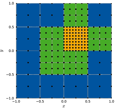
The Legendre-Gauss-Lobatto integration points of a second-order ($k=2$) DG method are indicated by the black dots. Note that on each edge there are actually two points stacked on each other, one for each adjacent cell to allow for discontinuous solutions.

Furthermore, as the PERK schemes can be cast into the framework of PRKM, one can utilize results on order conditions [18], conservation of linear invariants [19] and nonlinear stability properties [20, 21, 22, 23]. In [1, 2] the PERK schemes have been applied to static meshes for the simulation of the compressible Navier-Stokes equations. In this work, we apply the PERK schemes to dynamically refined meshes based on AMR which requires a dynamic re-assignment of the unknowns $\boldsymbol{u}$ to the corresponding integrators. We investigate whether speedup compared to other Runge-Kutta methods tailored to wave propagation and DG methods can be realized, despite the additional overhead due to the re-assignment. Besides considering viscous flows, we also apply the PERK schemes to purely hyperbolic problems.

This paper is structured as follows: First, we introduce the class of PRKM by revisiting central properties such as order of consistency, linear/absolute stability, internal consistency, conservation properties and criteria for nonlinear stability. Next, we briefly introduce the PERK methods devised by Vermeire with a special focus on showcasing issues related to nonlinear stability. As the PERK schemes can be constructed from optimized stability polynomials, we discuss the construction of the stability polynomials in Section 4 with an emphasis on the construction of the spectrum for which we propose an efficient algorithm. In Section 5 we briefly compare the PERK schemes to the composing standalone methods. Next, we turn our attention in Section 6 onto describing the implementation aspects of the partitioning and devising a measure for estimation of the effectiveness of the PERK schemes. Then, we present a range of classical testcases for both viscous and inviscid flows in Section 7 for which we provide a reproducibility repository [24]. Finally, Section 8 concludes the paper.

2 Partitioned Runge-Kutta Methods

In this work, we consider coefficient-based partitioned ode of the form

$$\boldsymbol{U}(t_{0}) =\boldsymbol{U}_{0}$$ (2.1a)

$$\boldsymbol{U}^{\prime}(t) =\begin{pmatrix}\boldsymbol{U}^{(1)}(t)\\ \vdots\\ \boldsymbol{U}^{(R)}(t)\end{pmatrix}^{\prime}=\begin{pmatrix}\boldsymbol{F}^{(1)}\big{(}t,\boldsymbol{U}^{(1)}(t),\dots,\boldsymbol{U}^{(R)}(t)\big{)}\\ \vdots\\ \boldsymbol{F}^{(R)}\big{(}t,\boldsymbol{U}^{(1)}(t),\dots,\boldsymbol{U}^{(R)}(t)\big{)}\end{pmatrix}=\boldsymbol{F}\big{(}t,\boldsymbol{U}(t)\big{)}$$ (2.1b)

where $R\in\mathbb{N}$ denotes the number of partitions which correspond to the levels of refinement in the context of quad/octree AMR, cf. Fig. 1. In the case of non-uniform meshes the partitioning of the semidiscretization (1.2) is based on the minimum edge length $h$ of the grid cells. For the DG method employed in this work, the coefficients of the local solution polynomials are the unknowns of the ode system (2.1) and can be uniquely assigned to a partition based on the minimum edge length $h$ of the associated cell. In the following, the superscript $(\cdot)^{(r)}$ indicates quantities corresponding to the $r$’th partition.

Systems of the form (2.1) motivate the usage of PRKM, which are given in Butcher form given by [25]

$$\boldsymbol{U}_{0} =\boldsymbol{U}(t_{0})$$ (2.2a)

$$\boldsymbol{K}_{i}^{(r)} =\boldsymbol{F}^{(r)}\left(t_{n}+c_{i}^{(r)}\Delta t,\boldsymbol{U}_{n}+\Delta t\sum_{j=1}^{S}\sum_{k=1}^{R}a_{i,j}^{(k)}\boldsymbol{K}_{j}^{(k)}\right),\quad r=1,\dots,R,\>\>i=1,\dots,S$$ (2.2b)

$$\boldsymbol{U}_{n+1} =\boldsymbol{U}_{n}+\Delta t\sum_{i=1}^{S}\sum_{r=1}^{R}b_{i}^{(r)}\boldsymbol{K}_{i}^{(r)}\,.$$ (2.2c)

Here, $S$ denotes the number of stages $\boldsymbol{K}_{i}$ and $a_{i,j}^{(r)}$ form the Butcher array matrix $A^{(r)}$.

PRKM have been introduced in the 1970s [26, 27] and have received notable usage for the integration of Hamiltonian systems [28, 29]. An essentially equivalent class of Runge-Kutta methods are ARKMs [30, 15, 31], which have been developed in order to achive efficient integration of multiscale and stiff systems [14, 15]. Similar works have been performed with PRKM [9, 7, 8]. Since the PERK methods we apply in this work are a special case of PRKM [2], we briefly revisit conditions for convergence order, absolute stability, conservation of linear invariants, internal consistency, and nonlinear stability.

2.1 Order Conditions

In addition to the classical conditions for convergence of order $p$, PRKM need to satisfy additional conditions which have been derived by multiple authors, see [27, 18, 32] and for a compact summary [33]. For identical abscissae $\boldsymbol{c}^{(r)}\equiv\boldsymbol{c}$ and weights $\boldsymbol{b}^{(r)}\equiv\boldsymbol{b}$ (more on this restriction below), these in principle additional order constraints reduce for $p=1,2,3$ conveniently to the classical ones:

$$p=1: \boldsymbol{b}^{T}\boldsymbol{1} \overset{!}{=}1$$ (2.3a)

$$p=2: \boldsymbol{b}^{T}\boldsymbol{c} \overset{!}{=}\frac{1}{2}$$ (2.3b)

$$p=3: \boldsymbol{b}^{T}\boldsymbol{c}^{2} \overset{!}{=}\frac{1}{3}$$ (2.3c)

$$\boldsymbol{b}^{T}A^{(r)}\boldsymbol{c} \overset{!}{=}\frac{1}{6}\quad\forall\>r=1,\dots,R\,.$$ (2.3d)

Here, $\boldsymbol{1}\in\mathbb{R}^{S}$ denotes the vector of ones and the exponentiation of vectors is to be understood element-wise.

For order $p=4$, however, even for identical abscissae $\boldsymbol{c}$ and weights $\boldsymbol{b}$ non-trivial coupling conditions between the Butcher arrays $A^{(r)}$ of the different methods arise [33], rendering the construction of an optimized fourth-order PERK scheme significantly more difficult. In the original publication [1] second-order PERK schemes are proposed which have then be extended to third-order in a subsequent work [2].

2.2 Absolute Stability

Absolute stability, or linear stability, examines the asymptotic behaviour of a time integration method applied to the constant-coefficient linear test system [34]

$$\boldsymbol{U}^{\prime}(t)=J\,\boldsymbol{U}(t).$$ (2.4)

In this work, $J$ corresponds to the Jacobian of the RHS $\boldsymbol{F}\big{(}t,\boldsymbol{U}(t)\big{)}$ (1.2)

$$J(t,\boldsymbol{U})\coloneqq\frac{\partial\boldsymbol{F}\big{(}t,\boldsymbol{U}(t)\big{)}}{\partial\boldsymbol{U}}.$$ (2.5)

A time-integration method is called absolutely stable if its associated stability function $P(z)$ (which is a polynomial for explicit methods) is in magnitude less or equal to one when evaluated at the scaled eigenvalues with non-positive real part

$$|P(\Delta t\lambda)|\overset{!}{\leq}1\quad\forall\>\lambda\in\boldsymbol{\sigma}(J):\text{Re}(\lambda)\leq 0\,.$$ (2.6)

In other words, we demand that the scaled spectrum lies in the region of absolute stability of the method with stability polynomial $P(z)$. Since the RHS $\boldsymbol{F}$ depends on the solution $\boldsymbol{U}$ itself, we require (2.6) to hold for all (unknown) states $\boldsymbol{U}(t)$ reached during the simulation. This is in principle difficult to ensure, but in practice the spectra $\boldsymbol{\sigma}\big{(}J(\boldsymbol{U})\big{)}$ are observed to be relatively similar to the spectrum of the initial condition $\boldsymbol{\sigma}\big{(}J(\boldsymbol{U}_{0})\big{)}$.

The linear stability properties of PRKM have been studied in [35] with special focus on separable Hamiltonian systems. For ARKMs, a linear stability analysis is performed in [31] based on the test problem $U^{\prime}=\sum_{r=1}^{R}\lambda^{(r)}U$.

For PRKM it is customary to investigate the test equation

$$\boldsymbol{U}^{\prime}=\Lambda\boldsymbol{U},\quad\Lambda\in\mathbb{C}^{N\times N}$$ (2.7)

which can be naturally partitioned according to a set of mask-matrices $I^{(r)}\in\{0,1\}^{N\times N}$:

$$\Lambda=\sum_{r=1}^{R}\Lambda^{(r)}=\sum_{r=1}^{R}I^{(r)}\Lambda\,.$$ (2.8)

The mask-matrices fulfill the property $\sum_{r=1}^{R}I^{(r)}=I$, with $I$ being the identity matrix of dimensions $N\times N$. The mask matrices $I^{(r)}$ are required to specify the exact partitioning of (2.1b):

$$\boldsymbol{U}(t) =\sum_{r=1}^{R}\underbrace{I^{(r)}\boldsymbol{U}(t)}_{\eqqcolon\boldsymbol{U}^{(r)}(t)}\,, \boldsymbol{F}\big{(}t,\boldsymbol{U}(t)\big{)}=\sum_{r=1}^{R}\underbrace{I^{(r)}\boldsymbol{F}\big{(}t,\boldsymbol{U}(t)\big{)}}_{\eqqcolon\boldsymbol{F}^{(r)}\big{(}t,\boldsymbol{U}(t)\big{)}}\,.$$ (2.9)

The matrix-valued stability function $P(Z)\in\mathbb{C}^{N\times N}$ is with $Z^{(r)}\coloneqq\Delta t\Lambda^{(r)}$ given by [19]

$$P(Z)=I+\left(\sum_{r=1}^{R}\left(\boldsymbol{b}^{(r)}\otimes I\right)^{T}\left(Z^{(r)}\otimes I\right)\right)\left(I_{NS}-\sum_{r=1}^{R}\left(A^{(r)}\otimes I\right)\left(Z^{(r)}\otimes I\right)\right)^{-1}(\boldsymbol{1}\otimes I).$$ (2.10)

where $\otimes$ denotes the Kronecker product and $I_{NS}$ the identity matrix of dimension $N\cdot S$. As discussed in [35], it is difficult to infer information on the linear stability of the overall partitioned scheme from (2.10) based on the stability properties of the individual schemes $(A^{(r)},b^{(r)})$ for arbitrary mask matrices $I^{(r)}$. In contrast to classic Runge-Kutta methods, one can for PRKM no longer solely infer the action of the time-integration scheme from the stability functions of the individual methods [35]. This issue returns in Section 3.2 when the nonlinear stability properties of a special class of PRKM are discussed.

In practice, however, it is observed that absolute stability of each method $(A^{(r)},\boldsymbol{b}^{(r)})$ for its associated spectrum $\boldsymbol{\lambda}^{(r)}$ suffices for overall linear stability, irrespective of the concrete realization of the mask matrices $I^{(r)}$ [1, 2]. To check this, one can either compute $P(Z)$ via (2.10) or set up the fully discrete system directly, i.e., apply the Runge-Kutta method to (2.4). Then, linear stability follows from applying stability criteria for discrete-time linear time-invariant systems [36]. This is illustrated for a concrete example in Section 3.2.2.

2.3 Internal Consistency

To ensure that the approximations of the partitioned stages $\boldsymbol{K}_{i}^{(r)}$ approximate indeed the same timesteps $c_{i}$ across partitions $r$, we require internal consistency [19, 22, 31], i.e.,

$$\sum_{j=1}^{i-1}a^{(r)}_{i,j}\overset{!}{=}c_{i}\quad\forall\>i=1,\dots,S\>\>\forall\>r=1,\dots,R\,,$$ (2.11)

which is equivalent to all $R$ Runge-Kutta methods having stage order one [19]. It has been demonstrated in [22, 19] that internal consistency is required to avoid spurious oscillations at the interfaces between partitions.

2.4 Conservation of Linear Invariants

Since the underlying PDE from which the semidiscretization (1.2) is constructed correspond oftentimes to conservation laws like (1.1) prescribing the conservation of mass, momentum, and energy it is natural to require that the application of a PRKM preserves this property for conservative spatial discretizations such as finite volume and DG schemes. For equation based partitioning according to (2.1b) this is ensured if the weights $\boldsymbol{b}$ are identical across partitions [10, 19], i.e.,

$$b_{i}^{(r_{1})}=b_{i}^{(r_{2})}=b_{i},\>\forall\>i=1,\dots,S,\>\>\forall\>r_{1},r_{2}=1,\dots,R\,.$$ (2.12)

For flux-based partitioning this restriction may be relaxed, see [23] for a detailed discussion.

2.5 Nonlinear Stability

Nonlinear stability includes (among stronger results for scalar equations) positivity preservation of physical quantities such as pressure and density and the suppression of spurious oscillations around discontinuities. Time integration methods guaranteeing these properties are termed ssp and have been well-studied over the past years [37, 38]. The nonlinear stability properties of partitioned/additive Runge-Kutta methods have been investigated in [20, 21, 22, 23]. In the aforementioned works it was shown that for an overall ssp PRKM the individual methods have to be ssp and the timestep $\Delta t$ is furthermore restricted by

$$\Delta t=\min_{r=1,\dots,R}\left\{c^{\text{SSP}}_{r}\right\}\Delta t_{\text{Forward Euler}}.$$ (2.13)

Here, $c^{\text{SSP}}_{r}$ denotes the ssp coefficient [38] (radius of absolute monotonicity [20, 39]) of the $r$’th method. Except for some special cases where the timestep is restricted due to absolute stability (see, e.g., [40]) 2.13 renders the application of ssp-capable PRKM in many cases ineffective, as the method with the smallest ssp coefficient determines the overall admissible timestep which guarantees nonlinear stability.

Having discussed the properties of PRKM, we now turn our attention to a special case thereof, namely the Paired-Explicit Runge-Kutta (P-ERK) methods proposed by Vermeire [1].

3 Paired-Explicit Runge-Kutta (P-ERK) Methods

Paired-Explicit Runge-Kutta (P-ERK) methods have been originally proposed in [1] and were extended to third-order in [2]. These schemes target systems which exhibit locally varying characteristic speeds, most prominently due to non-uniform grids. In the context of the DG schemes considered in this work, the local wave speeds depend both on the spectral radii $\rho_{i},i=1,\dots,N_{D}$ of the directional Jacobians $J_{i}=\partial_{\boldsymbol{u}}\boldsymbol{f}_{i},i=1,\dots,N_{D}$ of the flux function (1.1) and the local grid size $h_{i}$:

$$\text{CFL}\sim\min_{i=1,\dots,N_{D}}\frac{h_{i}}{(k+1)\cdot\rho_{i}}.$$ (3.1)

Here, $N_{D}\in\{1,2,3\}$ denotes the number of spatial dimensions and $k$ the local polynomial degree of the DG approximation. When applying an explicit time-integration method to the semidiscretization (1.2b) the maximum timestep $\Delta t$ is restricted according to

$$\Delta t\overset{!}{\leq}\beta\cdot\text{CFL}$$ (3.2)

where $\beta\in\mathbb{R}_{+}$ depends on the employed time-integration method. As discussed in Section 4 we seek to maximize this factor by optimizing the domain of absolute stability for the different methods.

Note that the estimate (3.1) is only a valid bound for the maximum timestep $\Delta t$ in the convection-dominated case, i.e., when the spectral radius $\rho$ of the Jacobian of the fully discrete system 1.2b $J_{\boldsymbol{F}}(\boldsymbol{U})$ scales as

$$\rho\sim\frac{|a|}{h}\gg\frac{|d|}{h^{2}}$$ (3.3)

where $h$ denotes the smallest characteristic cell size and $a,d$ are suitable quantifiers for the influence of convection and diffusion, respectively.

For such problems, one can partition the semidiscretization (1.2) according to the local CFL stability constraint. For each partition $r$, an optimized stability polynomial $P_{p;E^{(r)}}^{(r)}(z)$ of order $p$ and degree $E^{(r)}$ is constructed which is then used to derive a specific Runge-Kutta method $(A^{(r)},\boldsymbol{b}^{(r)})$. In particular, methods with more RHS evaluations $E$ and larger $\beta_{E}$ are used in regions with smaller CFL number, while methods with smaller $E$ and smaller region of absolute stability (smaller $\beta_{E}$) are used for the elements of larger size and higher CFL. This is illustrated in Fig. 1 where a three times refined grid using a quadtree refinement strategy is shown. This enables a more efficient time integration since the evaluations $E$ of the right-hand-side of (1.2b) are performed only in the regions where they are actually required, and saved in other parts of the domain. Most important, efficiency is gained only in the coarse regions of the mesh, where cheaper integrators are used instead of the expensive one used in the finest parts. This idea is conceptually similar to local time-stepping methods which perform additional operations only in the fine regions of the mesh by reducing the timestep locally [10, 11].

3.1 Introduction

To illustrate the concept of the PERK schemes, we present the Butcher Tableaus of the second-order accurate PERK method obtained from a four-stage and a six-stage method:

$$\begin{array}[]{c|c|c c c c c c|c c c c c c c c}i&\boldsymbol{c}&&&A^{(1)}&&&&&&A^{(2)}&&&&&\\ \hline\cr 1&0&&&&&&&&&&&&&&\\ 2&\nicefrac{{1}}{{10}}&\nicefrac{{1}}{{10}}&&&&&&\nicefrac{{1}}{{10}}&&&&&\\ 3&\nicefrac{{2}}{{10}}&\nicefrac{{2}}{{10}}&0&&&&&\nicefrac{{2}}{{10}}-a_{3,2}^{(2)}&a_{3,2}^{(2)}&&&&\\ 4&\nicefrac{{3}}{{10}}&\nicefrac{{3}}{{10}}&0&0&&&&\nicefrac{{3}}{{10}}-a_{4,3}^{(2)}&0&a_{4,3}^{(2)}&\\ 5&\nicefrac{{4}}{{10}}&\nicefrac{{4}}{{10}}-a_{5,4}^{(1)}&0&0&a_{5,4}^{(1)}&&&\nicefrac{{4}}{{10}}-a_{5,4}^{(2)}&0&0&a_{5,4}^{(2)}&&\\ 6&\nicefrac{{5}}{{10}}&\nicefrac{{5}}{{10}}-a_{6,5}^{(1)}&0&0&0&a_{6,5}^{(1)}&&\nicefrac{{5}}{{10}}-a_{6,4}^{(2)}&0&0&0&a_{6,4}^{(2)}&\\ \hline\cr&\boldsymbol{b}^{T}&0&0&0&0&0&1&0&0&0&0&0&1\end{array}$$ (3.4)

The first method $A^{(1)}$ requires only the computation of stages $\boldsymbol{K}_{1}^{(1)},\boldsymbol{K}_{4}^{(1)},\boldsymbol{K}_{5}^{(1)},\boldsymbol{K}_{6}^{(1)}$, i.e., four evaluations of $\boldsymbol{F}^{(1)}$ while the second method $A^{(2)}$ requires computation of all stages $\boldsymbol{K}_{i}^{(2)},i=1,\dots,6$, i.e., six evaluations of $\boldsymbol{F}^{(2)}$. When looking at the first method in isolation, it becomes a reducible [34] method, i.e., the stages $\boldsymbol{K}_{2}^{(1)},\boldsymbol{K}_{3}^{(1)}$ do not influence the final solution $\boldsymbol{U}_{n+1}^{(1)}$ and the Butcher tableau could be truncated to a four-stage method. In the context of PRKM, however, the second and third stage are required for an internally consistent cf., 2.11, update of the intermediate state $\boldsymbol{U}_{n}+\Delta t\sum_{j=1}^{S}\sum_{r=1}^{R}a_{i,j}^{(r)}\boldsymbol{K}_{j}^{(r)}$, see (2.2b).

This particular form of the Butcher tableaus (3.4) comes with three advantages: First, the PERK methods are low-storage, requiring only storage of two Runge-Kutta stages at a time. Second, the computational costs per stage are not increasing if higher stage methods are used, as always at most two previous stages are used for computing the next stage. Third, the sparse structure of both $A^{(r)}$ and $\boldsymbol{b}^{(r)}$ allows for a simplified computation of the coefficients from a certain stability polynomial. The PERK methods are clearly internally consistent and conservative, i.e., methods which satisfy (2.11) and (2.12), respectively. The restriction to shared timesteps $c_{i}$ and weights $b_{i}$ comes also with the advantage of significantly simplified order constraints [33, 25], cf. (2.3).

We remark that a different choices of abscissae $\boldsymbol{c}$ and weights $\boldsymbol{b}$ than presented in (3.4) following [1] are possible. One options is to use $c_{S}=1$ and $b_{1}=b_{S}=\nicefrac{{1}}{{2}}$ which in the $S=2$ case boils down to Heun’s method. Another compelling option is given by $c_{S}=\nicefrac{{2}}{{3}}$ and $b_{1}=\nicefrac{{1}}{{4}},b_{S}=\nicefrac{{3}}{{4}}$ which are known in the $S=2$ case as Ralston’s method which minimizes the truncation error [41]. The choice proposed in [1] corresponds for $S=2$ to the explicit midpoint method.

The stability polynomials corresponding to (3.4) are given by

$$P_{2;4}^{(1)}(z) =1+z+\frac{1}{2}z^{2}+\alpha_{3}^{(1)}z^{3}+\alpha_{4}^{(1)}z^{4}$$ (3.5a)

$$P_{2;6}^{(2)}(z) =1+z+\frac{1}{2}z^{2}+\alpha_{3}^{(2)}z^{3}+\alpha_{4}^{(2)}z^{4}+\alpha_{5}^{(2)}z^{5}+\alpha_{6}^{(2)}z^{6}.$$ (3.5b)

The first subscript of $P^{(r)}$ denotes the linear order of consistency $p$ of the method, while the second subscript denotes the degree of the polynomial which is equal to the number of RHS evaluations $E^{(r)}$.

The free coefficients $\boldsymbol{\alpha}^{(1)}\in\mathbb{R}^{2},\boldsymbol{\alpha}^{(2)}\in\mathbb{R}^{4}$ can be optimized for a certain spectrum $\boldsymbol{\sigma}\big{(}J_{\boldsymbol{F}}(\boldsymbol{U})\big{)}$ of the Jacobian $J_{\boldsymbol{F}}(\boldsymbol{U})$ (2.5). Using optimized stabilized Runge-Kutta methods further increases the efficiency of the scheme as the region of absolute stability can be closely adapted to the spectrum $\boldsymbol{\sigma}\big{(}J_{\boldsymbol{F}}(\boldsymbol{U})\big{)}$ [42]. For convection-dominated problems, cf. (3.3), the spectra $\boldsymbol{\sigma}\big{(}J_{\boldsymbol{F}}(\boldsymbol{U})\big{)}$ of the semidiscretization increases linearly with the smallest inverse grid size $\nicefrac{{1}}{{h}}$. At the same time, the largest possible timestep $\Delta t_{p;E}$ (in the sense of absolute stability) of an optimized $p$’th order, $E$ degree stability polynomial scales also (asymptotically) linearly with the degree = number of stage evaluations $E$ [43, 44, 42]. Consequently, the usage of an optimized $2E$ stage-evaluation Runge-Kutta method for the simulation of a convection-dominated PDE with smallest grid size $\frac{1}{2}h$ allows using the same timestep $\Delta t$ as the simulation of the same problem on grid size $h$ with an $E$ stage-evaluation scheme.

In contrast, for diffusion-dominated PDE, the spectral radius increases quadratically with the inverse of the grid size, cf. (3.3). Thus, for an efficient treatment of such problems the region of stability needs also to increase quadratically with the number of stages $S$, which is the case for Runge-Kutta-Chebyshev methods [45, 46] targeting exactly such problems. These methods, however, do not extend without special treatment (see for instance [47, 48]) significantly into the complex plane, thus bearing issues for the convection-induced complex eigenvalues. Consequently, we restrict ourselves in this work to convection-dominated problems for which the required number of stages increases only linearly while refining the mesh.

3.2 Nonlinear Stability Properties

The key element to the effectiveness of the PERK schemes is the fact that evaluations of the right-hand-side can be avoided in regions of the domain with accordingly reduced characteristic speeds. This, in turn, requires that the weight vector $\boldsymbol{b}$ is relatively sparse in order to be able to omit as many stage computations as possible. In the context of the previous example 3.4, it is clear that the computation of $\boldsymbol{K}^{(1)}_{2}$ and $\boldsymbol{K}^{(1)}_{3}$ can only be avoided if $b_{2}=b_{3}=0$.

The presence of zeros in the shared weight vector, however, renders the method non ssp as the requirement $\boldsymbol{b}^{(r)}>\boldsymbol{0},\,r=1,\dots R$ [21, 49, 39] (the inequality is to be understood component-wise) is violated for the PERK schemes. Consequently, the PERK schemes offer no guarantees in terms of nonlinear stability properties, and, in fact, we show in the remainder of this section that this leads to problems even in the simplest examples.

3.2.1 Linear Advection with Godunov’s Scheme

To illustrate potential issues with nonlinear stability, we consider the canonical first-order Finite Volume Godunov scheme applied to the 1D advection equation with smooth initial data

$$u_{t}+u_{x} =0,$$ (3.6a)

$$u_{0}(t_{0}=0,x) =1+\frac{1}{2}\sin(\pi x)$$ (3.6b)

on $\Omega=(-1,1)$ equipped with periodic boundaries. For a potentially non-uniform spatial discretization the semidiscretization (1.2) reads for Upwind/Godunov flux

$$\boldsymbol{U}_{0} =\boldsymbol{U}(t_{0})$$ (3.7a)

$$\frac{\text{d}}{\text{d}t}\boldsymbol{U}(t) =\underbrace{\begin{pmatrix}-\frac{1}{\Delta x_{1}}&0&\dots&0&\frac{1}{\Delta x_{1}}\\ \frac{1}{\Delta x_{2}}&-\frac{1}{\Delta x_{2}}&0&\dots&0\\ &\ddots&\ddots&\\ 0&\dots&0&\frac{1}{\Delta x_{N}}&-\frac{1}{\Delta x_{N}}\end{pmatrix}}_{\eqqcolon L}\boldsymbol{U}(t)\,,$$ (3.7b)

where

$$U_{i}(t)\coloneqq\frac{1}{\Delta x_{i}}\int_{x_{i-\nicefrac{{1}}{{2}}}}^{x_{i+\nicefrac{{1}}{{2}}}}u(t,x)\,\text{d}x,\quad i=1,\dots,N$$ (3.8)

denote the cell-averages. Applying a two-level ($R=2$) PRKM to 3.7b leads to the fully discrete system

$$\boldsymbol{U}_{n+1}=\underbrace{\begin{pmatrix}D^{(1)}(\Delta t,L)\\ D^{(2)}(\Delta t,L)\end{pmatrix}}_{\eqqcolon D}\boldsymbol{U}_{n}$$ (3.9)

which is equivalent to the matrix-valued stability function (2.10) with $R=2$ and specified mask matrices $I^{(1)},I^{(2)}$.

3.2.2 Linear Stability of the Fully Discrete System

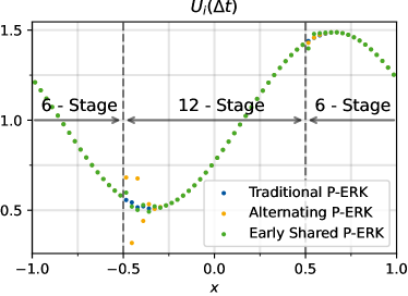
First, we consider an equidistant discretization with $N=64,\Delta x=\Delta x^{(1)}=\Delta x^{(2)}=\nicefrac{{2}}{{N}}$ where we use the optimized sixteen stage-evaluation method in the center of the domain, i.e., within $[-0.5,0.5]$, and the optimized eight stage-evaluation method in the remainder of the domain, see Fig. 3a. For the Godunov scheme, the spectrum $\boldsymbol{\sigma}\big{(}J(\boldsymbol{U})\big{)}$ is circular with center at $-a/\Delta x$ and radius $\rho=a/\Delta x$. For this spectrum the optimal stability polynomial for second-order accurate methods is known analytically for all polynomial degrees [44].

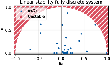
The solution $\boldsymbol{U}_{1}=\boldsymbol{U}(\Delta t)$ after one step with maximum stable timestep $\Delta t=0.21875$ is presented in Fig. 3a. Clearly, there are heavy oscillations at the interface between the two schemes. It is natural to ask whether these oscillations increase over time and cause a blow-up of the overall simulation. To answer this question, we consider the spectrum of $D$ (or equivalently $P(Z)$) which is also displayed in Fig. 2. In the present case the spectral radius $\rho(D)<1$ and thus the overall scheme is linearly stable [36], which is confirmed by long time runs. This shows that the observed oscillations are no consequence of violated linear/absolute stability, but instead are due to the nonlinear stability properties of the scheme which are explored in the next subsection.

Figure 2: Spectrum $\boldsymbol{\sigma}(D)$ of the fully discrete matrix $D$ of the $\text{P-ERK}_{2;\{8,16\}}$ scheme applied to (3.7b). The unstable region with $|\lambda|>1$ is shaded in red. Note that the purely real eigenvalue around $(1,0)$ is indeed stable with numeric value $1.0-28\varepsilon$ and machine epsilon $\varepsilon=\mathcal{O}\left(10^{-16}\right)$.

3.2.3 Nonlinear Stability of the Fully Discrete System

The fully discrete system (3.9) is monotonicity-preserving in the sense of Harten [50] if and only if

$$d_{ij}\geq 0\quad\>\forall\>i,j=1,\dots,N.$$ (3.10)

The application of the PERK schemes leads in general to a violation of (3.10), even for uniform meshes as clearly seen in Fig. 3a. To shed some more light on this, we present a plot of the matrix entries $d_{ij}$ in Fig. 3b.

(a) Result $\boldsymbol{U}_{1}$ of (3.9) after one step. The vertical dashed lines indicate the partitioning into $\boldsymbol{U}^{(1)}$ and $\boldsymbol{U}^{(2)}$.

(b) Non-zero entries $d_{ij}$ of fully-discrete system matrix $D$, cf. (3.9).

Figure 3: Cell averages $U_{i}(\Delta t)$ (Fig. 3a) after performing one timestep of the second-order 8-16 optimized PERK scheme applied to (3.7b) on a uniform mesh with $\Delta x=\nicefrac{{2}}{{64}}$. The entries of the fully discrete Matrix $D$ (cf (3.9)) are shown in Fig. 3b.

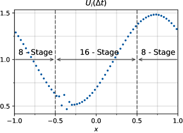
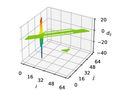
It is evident from Fig. 3b that monotonicity is lost at the intersection of the schemes, precisely where the higher-stage method retrieves only first-order data from the lower stage scheme. first-order information means in this case that the intermediate state $\boldsymbol{U}_{n}+\Delta t\sum_{i=1}^{S}\sum_{r=1}^{R}b_{i}^{(r)}\boldsymbol{K}_{i}^{(r)}$ (cf. (2.2b)) received on the $r=1$ partition only information from one evaluation of the RHS. In particular, the rows $i=17,\dots,24$ of $D$ have negative entries which originates from the fact that for these points the higher stage method still relies on first-order information only, precisely the previous iterate $\boldsymbol{U}_{n}$ plus the first stage $\boldsymbol{K}_{1}$. In particular, for the $S=16,E=\{8,16\}$ combination at stage $i=8$ the only update to $\boldsymbol{U}^{(1)}$ is due to $\left(c_{8}-a_{8,1}^{(1)}\right)\boldsymbol{K}_{8}^{(1)}$, while $\boldsymbol{U}^{(2)}$ receives an update including $a_{8,7}^{(2)}\boldsymbol{K}_{7}^{(2)}$ which contains seven consecutive evaluations of the RHS.

The influence of the negative entries can be clearly seen in Fig. 3a, where oscillations arise behind the transition from one scheme to the other. Since the initial condition is transported from the left to the right, the usage of the upwind fluxes corresponds to using information from the left. This is why there are oscillations in this case at $x=-0.5$, since the higher stage-evaluation method receives only first-order information based upon $\boldsymbol{K}_{1}^{(1)}$. At $x=0.5$ there are for positive advection velocity $a=1$ no oscillations, as the lower stage-evaluation method retrieves high order information at any time. In turn, for a negative transportation velocity, i.e., $u_{t}-u_{x}=0$ the oscillations arise at $x=0.5$.

We mention that each row sum $d_{i}\coloneqq\sum_{j=1}^{N}d_{ij}$ equals one, reflecting that the scheme is conservative, agreeing with the criteria (2.12). Furthermore, the PERK scheme converges with second-order once the asymptotic regime is reached.

This loss of monotonicity is noteworthy as it foreshadows possible problems for more complex scenarios. The first-order Godunov finite volume scheme is known to be very diffusive, yet already for this system and uniform meshes, artificial oscillations are introduced. There are several ways how the oscillations can be mitigated. First of all, the oscillations become less severe if the timestep is reduced since this leads to a reduction in magnitude of the negative entries $d_{ij}$. Next, for a higher spatial resolution $N$ the influence of the negative entries is reduced as neighboring values $U_{i}$ are of more similar value (note that no oscillations can occur for a constant solution since $d_{i}\coloneqq\sum_{j=1}^{N}d_{ij}=1$). Finally, the oscillations can also be reduced if the difference in the number of stage evaluations $E$ is reduced, with monotonicity recovered for the same method in each part of the domain. These observations are quantified in Section 3.2.5 for the intended application of the PERK schemes to non-uniform grids.

3.2.4 Alternative P-ERK Schemes

It is also instructive to consider a different stage evaluation pattern of the PERK methods. The original PERK methods perform all shared evaluations at the end, cf. (3.4). In principle, also different stage evaluation patterns are possible while preserving the key features of the PERK schemes. For instance, one can construct ”alternating” schemes such as

$$\begin{array}[]{c|c|c c c c c c}i&\boldsymbol{c}&&&A^{(1)}&&\\ \hline\cr 1&0&&&&&&\\ 2&\nicefrac{{1}}{{10}}&\nicefrac{{1}}{{10}}&&&&&\\ 3&\nicefrac{{2}}{{10}}&\nicefrac{{2}}{{10}}&0&&&&\\ 4&\nicefrac{{3}}{{10}}&\nicefrac{{3}}{{10}}-a_{4,3}^{(1)}&0&a_{4,3}^{(1)}&&&\\ 5&\nicefrac{{4}}{{10}}&\nicefrac{{4}}{{10}}&0&0&0&&\\ 6&\nicefrac{{5}}{{10}}&\nicefrac{{5}}{{10}}-a_{6,4}^{(1)}&0&0&a_{6,4}^{(1)}&0&\\ \hline\cr&\boldsymbol{b}^{T}&0&0&0&0&0&1\end{array}$$ (3.11)

from the same stability polynomial $P_{2;4}^{(1)}(z)$ (3.5) that would be used for the traditional PERK scheme (3.4). For the first scheme, specified according to (3.11), the stages $\boldsymbol{K}_{1}^{(1)},\boldsymbol{K}_{3}^{(1)},\boldsymbol{K}_{4}^{(1)},\boldsymbol{K}_{6}^{(1)}$ are evaluated, while for the classic PERK scheme (3.4) $\boldsymbol{K}_{1}^{(1)},\boldsymbol{K}_{4}^{(1)},\boldsymbol{K}_{5}^{(1)},\boldsymbol{K}_{6}^{(1)}$ are evaluated.

Another possible design pattern for PERK schemes is to perform the shared evaluations at the early stages of the method, rather than at the end as for the traditional PERK schemes. The Butcher Tableau for the $p=2$, $E=4,S=6$ scheme with this stage evaluation pattern is given by

$$\begin{array}[]{c|c|c c c c c c}i&\boldsymbol{c}&&A^{(1)}&&&\\ \hline\cr 1&0&&&&&&\\ 2&\nicefrac{{1}}{{10}}&\nicefrac{{1}}{{10}}&&&&&\\ 3&\nicefrac{{2}}{{10}}&\nicefrac{{2}}{{10}}-a_{3,2}^{(1)}&a_{3,2}^{(1)}&&&&\\ 4&\nicefrac{{3}}{{10}}&\nicefrac{{3}}{{10}}&0&0&&&\\ 5&\nicefrac{{4}}{{10}}&\nicefrac{{4}}{{10}}&0&0&0&&\\ 6&\nicefrac{{5}}{{10}}&\nicefrac{{5}}{{10}}-a_{6,3}^{(1)}&0&a_{6,3}^{(1)}&0&0&\\ \hline\cr&\boldsymbol{b}^{T}&0&0&0&0&0&1\end{array}$$ (3.12)

where the free coefficients $a_{3,2}^{(1)},a_{6,3}^{(1)}$ are again obtained from the identical stability polynomial $P_{2;4}^{(1)}(z)$ that may be used for the other methods. In this case, stages $\boldsymbol{K}_{1}^{(1)},\boldsymbol{K}_{2}^{(1)},\boldsymbol{K}_{3}^{(1)},\boldsymbol{K}_{6}^{(1)}$ are evaluated.

To illustrate the influence of the stage evaluation pattern Fig. 4 compares the results after one timestep for the standard 3.4, alternating 3.11, and shared early stage 3.12 PERK scheme. Clearly, the schemes yield different results at the interfaces at the schemes, with the strongest oscillations observed for the alternating scheme. Notably, the scheme with shared early stage evaluations causes the largest errors at the fine-coarse interface at $x=0.5$.

Analogous to the linear stability properties discussed in Section 2.2, the action of partitioned schemes is no longer determined by the stability polynomials of the individual schemes only, even for linear ode. In fact, due to the partitioning there is a discontinuity in the time-integration method introduced and consequently, the final outcome does depend on the design of the stage evaluation pattern.

This feature is similar in spirit to ssp time integration schemes. Consider for instance the two-stage second-order stability polynomial, for which infinitely many Runge-Kutta methods exist, for instance the midpoint method and Heun’s method mentioned earlier. When applied to a linear problem, both give the identical result, as the overall outcome is governed by the same stability polynomial. In contrast, when applied to a nonlinear, potentially discontinuous problem, the implementation of the intermediate stage is of crucial importance as this determines the nonlinear stability properties, see the instructive example given in [51].

Figure 4: Result $\boldsymbol{U}^{1}$ to 3.9 after one timestep of two different 6-12 PERK schemes with different stage evaluation patterns on a uniform mesh. The solution colored in blue correspond to the standard PERK scheme (3.4) while the solution obtained with the alternating PERK scheme (3.11) is colored in orange.

3.2.5 Non-uniform Meshes

Coming to the intended application case of the PERK schemes to non-uniform meshes, it is observed that the presence of a discontinuity in the system matrix $L$ (3.7b) further impairs nonlinear stability. To give evidence for this, we consider again the model problem (3.6) and refine the grid in $\Omega^{(2)}\coloneqq[-0.5,0.5]$ by a factor $\alpha>1$, i.e., $\Delta x_{2}=\Delta x_{1}/\alpha$. In the non-refined part of the mesh with $\Delta x_{1}=\nicefrac{{2}}{{64}}$ an $E^{(1)}=8$ stage-evaluation method is used, while in the refined part the number of stage evaluations is determined based on $\alpha$ such that the timestep $\Delta t_{8}=0.21875$ can be kept constant. For all configurations presented in this section linear stability was checked by means of the spectral radius of the fully discrete system matrix $D$ (3.9) and long-time simulations.

To measure the oscillations, we consider the relative total variation (TV) increase after one timestep

$$e^{\text{TV}}\coloneqq\frac{\|\boldsymbol{U}_{1}\|_{\text{TV}}-\|\boldsymbol{U}_{0}\|_{\text{TV}}}{\|\boldsymbol{U}_{0}\|_{\text{TV}}}$$ (3.13)

with total variation seminorm $\|\boldsymbol{U}\|_{\text{TV}}\coloneqq\sum_{i}|U_{i+1}-U_{i}|$. $e^{\text{TV}}$ is reported in Table 1 for a range of stage evaluations $E^{(2)}$ in the refined region. Only for the most modestly refined grid the total variation actually decreases, preserving the diffusive nature of the Godunov scheme. For higher refinement ratios, exponential increase in total variation is observed, with dramatic values for the highest refinements.

$E^{(2)}$	9	10	11	12	13	14	15	16
$\alpha$	1.125	1.25	1.375	1.5	1.625	1.75	1.875	2.0
$e^{\text{TV}}$	$\boldsymbol{-}0.03$	$0.11$	$0.55$	$1.65$	$3.71$	$7.85$	$15.4$	$26.0$

Table 1: Increase in relative total variation $e_{\,\text{TV}}$ for non-uniform meshes with grid sizes $\Delta x,\frac{\Delta x}{\alpha}$. The $E^{(1)}=8$ method is used in the non-refined region for all $\alpha$.

Similar to the case for uniform grid with partitioned schemes, the oscillations decrease with a reduction in timestep, increase in spatial resolution, and smaller difference in the number of stage evaluations $E^{(2)}-E^{(1)}$. To illustrate this, we reduce the maximum stable timestep $\Delta t_{8}$ by a factor $\text{CFL}\leq 1$ and provide the increase in total variation in Table 2

CFL	$0.4$	$0.5$	$0.6$	$0.7$	$0.8$	$0.9$	$1.0$
$e^{\text{TV}}$	$-0.01$	$0.03$	$0.28$	$1.21$	$4.04$	$11.5$	$26.0$

Table 2: Increase in relative total variation $e_{\,\text{TV}}$ for non-uniform meshes with varying base grid size $\Delta x^{(1)}=\nicefrac{{2}}{{64}}$ and two times ($\alpha=2$) finer grid in $\Omega^{(2)}=[-0.5,0.5]$ under reduction of timestep $\Delta t=\text{CFL}\cdot\Delta t_{8}$. The coarse cells are integrated with the $E^{(1)}=8$ stage evaluation method, while the fine cells are integrated using the $E^{(2)}=16$ method.

Next, the base resolution $N^{(1)}$, i.e., the resolution in $\Omega^{(1)}\coloneqq(-1,-0.5]\cup[0.5,1)$ is varied from $N^{(1)}=64$ to $N^{(1)}=4095$ for the $E^{(1)}=8,E^{(2)}=16$ scheme. As tabulated in Table 3 the increased resolution causes the increase in total variation to diminish on finer grids.

$N^{(1)}$	64	128	256	512	1024	2048	4096
$e^{\text{TV}}$	$26.0$	$7.27$	$1.82$	$0.45$	$0.11$	$0.02$	$0.01$

Table 3: Increase in relative total variation $e_{\,\text{TV}}$ for non-uniform meshes with varying base grid size $\Delta x_{\text{Base}}=\nicefrac{{2}}{{N^{(1)}}}$ and two times ($\alpha=2$) finer grid in $\Omega^{(2)}=[-0.5,0.5]$. The coarse cells are integrated with the $E^{(1)}=8$ stage evaluation method, while the fine cells are integrated using the $E^{(2)}=16$ method.

Finally, keeping cell size $\Delta x^{(1)}=\frac{2}{64}$ and ratio $\alpha=2$, the difference in stage evaluations $\Delta E=E^{(2)}-E^{(1)}$ is varied. Here, we always set $E^{(2)}=2E^{(1)}$ which implies that $\Delta E=E^{(2)}-E^{(1)}=2E^{(1)}-E^{(1)}=E^{(1)}$. For smaller $\Delta E$ the increase in total variation is reduced, as shown in Table 4. This can be intuitively explained by the fact that for smaller $\Delta E$ the higher stage method does less stages with only first-order information based on $\boldsymbol{K}_{1}^{(1)}$ from the lower stage method.

$\Delta E=E^{(1)}$	2	3	4	5	6	7	8
$e^{\text{TV}}$	$-0.00$	$-0.01$	$-0.00$	$0.06$	$0.61$	$4.25$	$26.0$

Table 4: Increase in relative total variation $e^{\text{TV}}$ for non-uniform meshes with constant base grid size $\Delta x^{(1)}=\nicefrac{{2}}{{64}}$ and two times ($\alpha=2$) finer mesh in $\Omega^{(2)}=[-0.5,0.5]$ under variation of the number of base stage evaluations $E^{(1)}=\{2,\allowbreak 3,\allowbreak 4,\allowbreak\dots,\allowbreak 8\}$. The fine cells are integrated using the $E^{(2)}=2E^{(1)}$ stage-evaluation method.

Since these issues are encountered for the Godunov scheme which evolves the cell averages, it is immediately clear that conventional limiting procedures are not applicable to remedy the loss of monotonicity. In particular, derivates of standard procedures such as MUSCL-type limiters [52] or related techniques to enforce, e.g., positivity [53] do not work as the mean state is already corrupted and therefore cannot be used as a fallback solution. In contrast, one would need to devise some form of flux limiting (or in this case stage-limiting) similar to techniques employed for the Lax-Wendroff scheme [52, 3], which also evolves cell averages.

3.2.6 Relation of Nonlinear Stability Analysis to Published Results

We would like to classify the previous observations in the context of the published results on PERK schemes. In [1, 2] the PERK schemes have been successfully applied to the simulation of the compressible Navier-Stokes equations for applications such as flows around airfoils. The meshes employed in the aforementioned works are characterized by a high resolution and small refinement rations between neighboring elements. For instance, the mesh for the simulation of a turbulent flow around the SD7003 airfoil employed in [2] has an average refinement ratio of $\bar{\alpha}\approx 1.15$. As illustrated by Table 1 moderate refinement ratios are much less vulnerable to monotonicity violations. As the refinement ration of neighboring cells is typically small, the difference in stage evaluations $E^{(r+1)}-E^{(r)}$ may also be relatively small. In fact, in [1, 2] the authors use PERK families with a maximum difference in stage evaluations of $\Delta E=4$. Again, we demonstrated by means of Table 4 that the monotonicity violations are reduced for smaller $\Delta E$. In conjunction with the fact that the simulated equations bear a diffusive nature, the potential loss of monotonicity is not observed in the aforementioned works.

Besides presenting application to the compressible Navier-Stokes equations, the inviscid isentropic vortex advection test case [37, 54] is also studied in [1, 2] for the purpose of validating the PERK schemes. Notably, they employ a random distribution of PERK schemes on a uniform grid to test the order of convergence of the schemes. For this test case it is in principle possible that the $E^{(R)}=16$ scheme is placed next to an $E^{(1)}=2$ (for the second-order accurate case) or $E^{(1)}=3$ (for the third-order accurate case) scheme. Based on the findings in the previous section one might expect that this could reveal the loss of monotonicity described in the previous section. This is not the case, however, as the timestep has to be adapted to the scheme with the smallest number of stage evaluations which requires a significant reduction in timestep. For instance, the maximum stable timestep for the $p=3,E=3$ scheme is about 8 times smaller than the one for the $p=3,E=16$ scheme. As tabulated in Table 2 there are no artificial oscillations observed if the timestep is chosen small enough.

To further strengthen the assessment discussed above, we created a test case based on a structured, smoothly refined, high-resolution mesh where we use a second-order, 16-stage PERK scheme with stage evaluations $E=\{4,6,8,\dots,16\}$. In agreement with the analysis above, this testcase can be run without reduction of the timestep for increased stage evaluations $E^{(R)}$, i.e., the stage normalized timestep $\Delta t/E^{(R)}$ can be kept almost constant for all schemes. This application is presented in more detail in A. However, we would like to stress that the use case considered in this work is different from the one considered in [1, 2] and in A, as for quad/octree AMR the mesh refinement ratio is always a factor of two and thus the difference in stage evaluations $E^{(r)}-E^{(r-1)}$ grows exponentially with the number of refinement levels.

3.3 Higher-Order P-ERK Methods

In the original paper [1] PERK schemes of order $p=2$ are presented which are extended to order $p=3$ in [2]. A particular feature of Runge-Kutta methods is that, given a certain stability polynomial, infinitely many Runge-Kutta methods with corresponding Butcher arrays can be constructed. For the third-order PERK methods, the proposed archetype of the Butcher tableau is [2]

$$\begin{array}[]{c|c c c}0&&\\ \frac{1}{3}&\frac{1}{3}&\\ 1&-1&2\\ \hline\cr&0&\frac{3}{4}&\frac{1}{4}\end{array}$$ (3.14)

which corresponds to the third-order Runge-Kutta method presented in [55] with parameter $c_{2}=\frac{1}{3}$. The presence of the negative entry $a_{3,1}=-1$ renders the incorporation of the $E=3,p=3$ in a PERK ensemble unattractive as the negative entry corresponds essentially to downwinding the numerical fluxes of stage $\boldsymbol{K}_{1}$ [51]. Alternatively, we choose the Butcher array of the canonical three-stage, third-order method by Shu and Osher [37] as the base scheme for our $p=3$ PERK schemes, i.e.,

$$\begin{array}[]{c|c c c}0&&\\ 1&1&\\ \frac{1}{2}&\frac{1}{4}&\frac{1}{4}\\ \hline\cr&\frac{1}{6}&\frac{1}{6}&\frac{4}{6}\end{array}$$ (3.15)

We emphasize that the usage of the first Runge-Kutta stage $\boldsymbol{K}_{1}$ in the final update step does not increase storage requirements of the scheme as $\boldsymbol{K}_{1}$ is used anyways to compute the higher stages, cf. (3.4). Also, the computational costs per stage stay at two scalar-vector multiplications and one vector-vector addition.

We have not yet discussed how to choose the free abscissae $c_{i},i=2,\dots,S-2$. In this work, we set

$$c_{i}=\frac{i-1}{S-3},\quad i=1,\dots,S-2$$ (3.16)

which corresponds to a linear distribution of timesteps between $c_{1}=0$ and $c_{S-2}=1$, similar to the second-order case [1]. We mention that more sophisticated choices of the abscissae are in principle possible, e.g., to improve the internal stability properties of the scheme [56]. Since this is not easily done and becomes also more relevant for many-stage methods which are not the main focus of this work, we restrict ourselves in this work to the linear distribution according to (3.16). Additionally, in contrast to the second-order accurate method, a nonlinear solver is required to obtain the $a_{i,i-1}$ from the coefficients $\alpha_{j}$ of the stability polynomial. Although in principle not guaranteed, with the choice of abscissae (3.16) we obtain positive Butcher coefficients $a_{i,i-1}$ for all optimized stability polynomials considered in this work.

As mentioned in Section 2.1 the construction of a fourth order PERK scheme is significantly more complex due to the coupling conditions involving the different Butcher arrays $A^{(r)}$ and is left for future research.

4 Construction of the Stability Polynomials

Besides their multirate property an additional advantage of the PERK schemes is that the stability polynomials of the constituting schemes can be optimized according to the intended application to maximize the admissible timestep $\Delta t$. In particular, we can construct stability polynomials that are tailored to the problem at hand, i.e., the spatial discretization, boundary and initial conditions. The optimization problem for the $p$’th order, $E^{(r)}$ degree stability polynomial thus reads

$$\max\Delta t\quad\text{s.t. }\left|P^{(r)}_{p;E^{(r)}}(\Delta t\lambda)\right|\leq 1,\>\forall\>\lambda\in\boldsymbol{\sigma}\,.$$ (4.1)

In the following, we first describe how the relevant eigenvalues of the spectrum $\boldsymbol{\sigma}$ are obtained and then discuss the solution of the optimization problem (4.1).

4.1 Generating Jacobian and Spectrum

Throughout this work we use Trixi.jl [57, 58, 59], a high-order DG code written in Julia for the numerical simulation of conservation laws. Trixi.jl supports algorithmic differentiation (AD) which allows exact and efficient computation of the Jacobian $J(\boldsymbol{U})$ (2.5). As long as memory requirements are no concern, the Jacobian can be computed quickly even for relatively large ode systems (1.2). In contrast, the eigenvalue decomposition to obtain the spectrum $\boldsymbol{\sigma}\big{(}J(\boldsymbol{U})\big{)}$ is computationally infeasible for practical simulation setups with millions of DoFs. At the same time, for the optimization of a stability polynomial the entire spectrum is not required. Instead, it suffices to supply a subset of the eigenvalues forming the boundary of the spectrum [58, 60]. To obtain this subset of eigenvalues lying on the boundary of the spectrum efficiently, we employ the following routine:

1. Compute $\widetilde{\boldsymbol{\sigma}}\left(\widetilde{J}(\boldsymbol{U}_{0})\right)$ for a semidiscretization $\boldsymbol{U}^{\prime}=\widetilde{\boldsymbol{F}}(\boldsymbol{U})$ with reduced minimal spatial resolution $\widetilde{h}$ such that the complete eigenvalue decomposition is still computational feasible. In this work, we use reduced systems with dimensionality $\mathcal{O}\left(10^{3}\times 10^{3}\right)$.

2. Compute the convex hull $\widetilde{\boldsymbol{\mu}}\left(\widetilde{\boldsymbol{\sigma}}\right)$ of the reduced spectrum $\widetilde{\boldsymbol{\sigma}}$. As the convex hull points can be quite distant from each other, additional points on the polygons are added such that the distance between two points is below the average distance $\delta$ between hull-points $\delta\coloneqq\sum_{k=1}^{K-1}\frac{\|\tilde{\mu}_{k+1}-\tilde{\mu}_{k}\|_{2}}{K-1}$.

   It suffices to consider either the second or third quadrant of the complex plane due to symmetry of $\boldsymbol{\sigma}$ with respect to the real axis. This also assumes that there are no amplifying modes with $\text{Re}(\lambda)>0$ in the spectrum, which is the case for the semidiscretizations arising from conservation laws considered in this work.

3. Increase the spatial resolution to the actual value used in the simulation, or the maximum value for which $J(\boldsymbol{U}_{0})$ can still be stored in main memory. Convert $J(\boldsymbol{U}_{0})$ to sparse format to save memory and computational costs for the subsequent Arnoldi iterations. For the DG discretizations considered here, $J(\boldsymbol{U}_{0})$ is typically extremely sparse due to the small DG stencils. As a side-node, ideally one would compute $J(\boldsymbol{U}_{0})$ already in sparse format. This, however, requires special techniques to identify the nonzeros (matrix-coloring) in the Jacobian which are not yet supported in Trixi.jl.

4. As discussed in Section 3.1 the spectrum of convection-dominated PDE scales increases linearly with decreasing characteristic grid size $h$. Consequently, the convex hull $\widetilde{\boldsymbol{\mu}}\in\mathbb{C}^{K}$ of the reduced spectrum is scaled by $\nicefrac{{\widetilde{h}}}{{h}}$ to agree with the discretization $\boldsymbol{U}^{\prime}=\boldsymbol{F}(\boldsymbol{U})$.

   Then, the ‘outer‘ eigenvalues of $J(\boldsymbol{U}_{0})$ can be estimated by performing Arnoldi iterations with shift $\mu_{k}\coloneqq\frac{\widetilde{h}}{h}\widetilde{\mu}_{k}$ to compute estimates to the eigenvalues close to the convex hull point $\mu_{k}$. This can be done efficiently as the Arnoldi iterations for the different hull points $\mu_{k},k=1,\dots,K$ can be parallelized. Furthermore, as the Arnoldi iteration involves only matrix-vector products, this approach heavily benefits from storing $J(\boldsymbol{U}_{0})$ in sparse format. Moreover, the stopping tolerance can be set relatively high as an estimate to the spectrum $\boldsymbol{\sigma}\left(J(\boldsymbol{U}_{0})\right)$ is not only sufficient, but in fact beneficial since $\widetilde{\boldsymbol{\sigma}}\left(J(\boldsymbol{U})\right)$ changes over the course of the simulation. This leads to an overall more robust stability polynomial. In terms of software we use Arpack.jl, a Julia wrapper around arpack-ng [61].

   In this work, we try to estimate the outer shape of the spectrum with 1000 eigenvalues, hence supplying to each Arnoldi iteration a target number of $M\coloneqq\nicefrac{{1000}}{{K}}$ eigenvalues. In general, after combining the estimates $\boldsymbol{\lambda}_{k}$ one will have less than 1000 distinct eigenvalues as some eigenvalues are found from multiple different shifts $\mu_{k}$. In practice, this still gives a sufficient large set of eigenvalues $\boldsymbol{\lambda}=\cup_{k=1}^{K}\boldsymbol{\lambda}_{k}$.

5. If also in step 3 a reduced system had to be considered (for instance due to memory restrictions), scale the obtained eigenvalues $\boldsymbol{\lambda}$ accordingly.

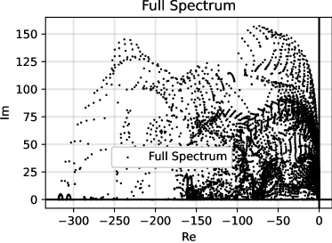
To illustrate the advantages of the presented routine, the reduced spectrum and the complete spectrum computed through a standard eigendecomposition are presented in Fig. 5. The spectrum shown in this case corresponds to the initial condition leading to a Kelvin-Helmholtz instability (see [62] for the precise setup) with the dgsem [63, 64] with flux-differencing [65, 66] using solution polynomials of degree $k=3$, hlle surface-flux [67], subcell shock-capturing [68] to suppress spurious oscillations, and entropy-conserving volume flux [69, 70]. Clearly, the shape of the spectrum is captured very well by the reduced spectrum while being significantly faster to compute. Furthermore, by estimating the spectrum using the procedure outlined above, one automatically obtains a reduced spectrum that captures the essential information while speeding up the subsequent optimization of the stability polynomial (discussed in the next section) as there are fewer redundant constraints to be checked. In this case, the shifts $\widetilde{\mu}_{k}$ are obtained from a reduced system with $\widetilde{J}\in\mathbb{R}^{1024\times 1024}$ for which the eigendecomposition can be performed in $0.4$ seconds. The large system is for the purpose of this study chosen such that the full eigendecomposition can still performed in somewhat reasonable time. Here, we consider $J\in\mathbb{R}^{16384\times 16384}$ where the full eigendecomposition takes more than $11$ minutes to complete. In contrast, for $K=20$ scaled shifts the Arnoldi iterations require in total only about $30$ seconds to complete. Here, $|\boldsymbol{\lambda}|=930$ distinct eigenvalues were found which are displayed in Fig. 5a.

(a) Reduced spectrum obtained from the procedure described in Section 4.1.

(b) Full spectrum obtained from standard eigendecomposition.

Figure 5: Reduced spectrum obtained from Arnoldi iterations around shifts (Fig. 5a) and full spectrum obtained from standard eigendecomposition (Fig. 5b). The spectrum corresponds to a dgsem discretization of the compressible Euler equations with an initial condition leading to a Kelvin-Helmholtz instability.

4.2 Optimization of the Stability Polynomial

Equipped with a set of constraining eigenvalues, it remains to find stability polynomials of prescribed degrees $E^{(r)}$ and linear order $p$ which maximize the stable timestep $\Delta t$. For this, we use the procedure developed in [42] which allows (in standard double precision) for an efficient and reliable optimization of general stability polynomials up to, say, degree 16. In principle, also the optimization of higher-degree polynomials is possible if a suitable basis, i.e., different from the monomials $z^{j}$ can be found for the spectrum of interest. While this is possible for simple cases like parabolic (negative real axis), purely hyperbolic (imaginary axis) and circle/disk spectra, the choice of the basis for the general case is unclear [42].

In the case of quad/octree-based AMR the characteristic cell size is halved with every level of refinement. This implies in the case of convection-dominated spectra (3.3) that the stable timestep needs to be reduced by a factor two, or, in the case of stabilized Runge-Kutta methods, that the number of stage-evaluation needs to be doubled.

Hence, for an $R$-times refined grid, one needs to construct stability polynomials with degrees up to $S^{(R+1)}=S^{(1)}\cdot 2^{R}$, i.e., the polynomial degree scales exponentially in the number of grid refinements $R$. As mentioned above, the optimization approach developed in [42] is for general spectra (for which no special suited basis can be found) not capable of reliably optimizing such high degree polynomials. Through employing a different ansatz for the optimization, one can optimize stability polynomials for convection dominated spectra with degrees larger than 100 [60].

Thus, we have in principle the possibility to integrate four to five times refined meshes with the same timestep as used for the base discretization. However, as discussed in Section 3.2 the nonlinear stability properties of PERK schemes worsen quickly for an increasing difference in stage evaluations $\Delta E^{(r+1)}\coloneqq E^{(r+1)}-E^{(r)}$, cf. Table 4. This renders the application of PERK schemes with stage evaluations $E^{(r)}=E^{(1)}\cdot\{1,\allowbreak 2,\allowbreak 4,\allowbreak 8,\allowbreak 16,...\}$ very inefficient, as the overall timestep needs to be reduced due to the poor nonlinear stability properties. As a consequence, we will restrict ourselves for practical cases presented in Section 7 to few-stage PERK families.

5 Validation

Before coming to applications we seek to compare the combined PERK schemes to standalone optimized schemes with regard to errors and conservation properties. For this, we consider the classic isentropic vortex testcase [37, 54] with the same parameters as used in [1, 2], except that here we use a more compact domain $\Omega=[0,10]^{2}$. In addition to the convergence studies presented in [1, 2] we compare the errors of the PERK schemes to the errors of an individual scheme. This information is essential for assessing the effectiveness of the PERK schemes since one is ultimately interested in accuracy per computational cost. For this testcase, the domain is initially discretized with 64 elements per direction, on which the solution is reconstructed using polynomials with degrees two (for second-order PERK scheme) and three (for third-order PERK scheme). The mesh is dynamically refined around the vortex based on the distance to the center of the vortex with two additional levels of refinement, i.e., the minimal grid size is in this case $h=\frac{10}{256}$. The numerical fluxes are computed using the hllc flux [71]. For solution polynomials of degree $k=2$ we construct $p=2$ optimal stability polynomials with degrees $3,6,$ and $12$, while for solution polynomials of degree $k=3$, $p=3$ stability polynomials of degrees $4,8$, and $16$ are optimized. We choose this particular PERK families since the presence of the additional free parameter allows the optimization of the lowest-degree stability polynomials, i.e., $P_{2;3}(z),P_{3;4}(z)$, to the spectrum.

The density errors at final time $t_{f}=20$

$$e_{\rho}(x,y)\coloneqq\rho(t_{f},x,y)-\rho_{h}(t_{f},x,y)$$ (5.1)

are tabulated in Table 5 for each individual optimized Runge-Kutta method and the composed PERK scheme.

Method	$\frac{1}{|\Omega|}\|e_{\rho}(x,y)\|_{L^{1}(\Omega)}$	$\|e_{\rho}(x,y)\|_{L^{\infty}(\Omega)}$
$\text{P-ERK}_{2;3}$	$1.77\cdot 10^{-5}$	$6.43\cdot 10^{-4}$
$\text{P-ERK}_{2;6}$	$1.77\cdot 10^{-5}$	$6.40\cdot 10^{-4}$
$\text{P-ERK}_{2;12}$	$1.74\cdot 10^{-5}$	$6.30\cdot 10^{-4}$
$\text{P-ERK}_{2;\{3,6,12\}}$	$2.09\cdot 10^{-5}$	$5.86\cdot 10^{-4}$
$\text{P-ERK}_{3;4}$	$4.05\cdot 10^{-7}$	$1.12\cdot 10^{-5}$
$\text{P-ERK}_{3;8}$	$4.05\cdot 10^{-7}$	$1.12\cdot 10^{-5}$
$\text{P-ERK}_{3;16}$	$4.05\cdot 10^{-7}$	$1.11\cdot 10^{-5}$
$\text{P-ERK}_{3;\{4,8,16\}}$	$3.73\cdot 10^{-7}$	$1.36\cdot 10^{-5}$

Table 5: Density-errors for isentropic vortex advection testcase after one pass through the domain $\Omega=[0,10]^{2}$ at $t_{f}=20$. The compressible Euler equations are discretized using the dgsem with hllc flux [71] on a dynamically refined mesh with cell sizes ranging from $\Delta x^{(1)}=\nicefrac{{10}}{{64}}$ to $\Delta x^{(3)}=\nicefrac{{2}}{{256}}$. For Runge-Kutta order $p=2$, the local polynomials are of degree $k=2$ while for Runge-Kutta order $p=3$ the solution is constructed using $k=3$ polynomials.

Both $L^{\infty}$ and domain-normalized $L^{1}$ errors are for the joint PERK schemes of similar size as the errors of the individual schemes. Especially the fact that there is no increase in $L^{\infty}$ norm shows that the PERK schemes can be used in practical simulations despite their poor nonlinear stability properties.

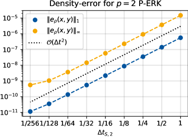
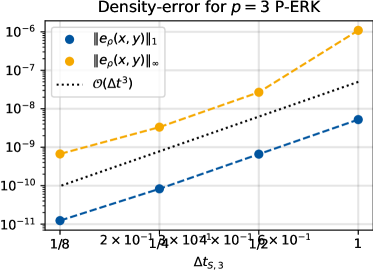
In [19] it is shown that at the interfaces of different schemes order reduction [72] may be encountered. As argued in [19], the interfaces between methods act like additional time-dependent internal boundary conditions, thus potentially suffering from effects also encountered for non-periodic problems [72]. Nevertheless, for both $L^{1}$ and $L^{\infty}$ error, both second and third-order PERK schemes display the expected order of convergence, as illustrated in Fig. 6. As in [1, 2], we employ local polynomials of degree $k=6$ for the convergence tests for both second and third-order PERK to minimize spatial errors.

(a) Density errors for second-order $E=\{3,6,12\}$ PERK family.

(b) Density errors for third-order $E=\{4,8,16\}$ PERK family.

Figure 6: $L^{1}$ and $L^{\infty}$ density errors for second (Fig. 6a) and third-order (Fig. 6b) PERK schemes applied to the isentropic vortex advection testcase. We observe the expected order of convergence for both second and third-order PERK schemes until the spatial discretization error dominates the overall error. This becomes especially visible for the $L^{\infty}$ errors plotted in orange.

It remains to examine whether the application of PERK schemes causes additional violation of the conserved fields compared to a standard Runge-Kutta scheme. For this purpose the third-order PERK scheme is compared against the three stage, third-order ssp method by Shu and Osher. As for the comparison of the density-errors of the PERK schemes to standalone schemes, the local polynomials are of degree $k=3$. The conservation error

$$e_{u}^{\text{Cons}}(t_{f})\coloneqq\left|\int_{\Omega}u(t_{0},\boldsymbol{x})\text{d}\boldsymbol{x}-\int_{\Omega}u(t_{f},\boldsymbol{x})\text{d}\boldsymbol{x}\right|$$ (5.2)

is computed for mass, momentum and energy after one pass of the vortex through the domain and tabulated in Table 6.

	$\text{P-ERK}_{3;\{4,8,16\}}$	$\text{SSP}_{3;3}$
$e_{\rho}^{\text{Cons}}(t_{f})$	$3.94\cdot 10^{-13}$	$7.82\cdot 10^{-13}$
$e_{\rho v_{x}}^{\text{Cons}}(t_{f})$	$4.79\cdot 10^{-14}$	$4.89\cdot 10^{-13}$
$e_{\rho v_{y}}^{\text{Cons}}(t_{f})$	$7.11\cdot 10^{-14}$	$5.00\cdot 10^{-13}$
$e_{\rho e}^{\text{Cons}}(t_{f})$	$1.06\cdot 10^{-12}$	$3.64\cdot 10^{-12}$

Table 6: Conservation-errors for isentropic vortex advection testcase after one pass through the domain at $t_{f}=20$ for the third-order PERK scheme and the three-stage, third-order Shu-Osher scheme.

Clearly, the errors of the $p=3,E=\{4,8,16\}$ PERK family are on par with the errors for the Shu-Osher scheme. In particular, these conservation violations are dominated by the spatial accuracy, i.e., reducing the timestep has very little influence. We also compared the $p=2,E=\{3,6,12\}$ PERK family to the two-stage second-order ssp scheme (Heun’s method) for a discretization with $k=2$ solution polynomials. For this configuration the conservation errors are negligible, both for the PERK and $\text{SSP}_{2;2}$ scheme.

All presented results from this section can be reproduced using the publicly available repository [24].

6 Methodology

In this section, we outline the procedure for the application of PERK schemes to simulations with quad/octree-based AMR in Trixi.jl.

6.1 Implementation

For obtaining the spatial semidiscretization (1.2) we use the dgsem [63, 64] with flux-differencing [65, 66] as implemented in Trixi.jl. To demonstrate that indeed no changes to the spatial discretization are required, we exemplary provide the standard implementation of the volume integral computation in Trixi.jl in LABEL:listing:Trixi and the implementation used for the PERK schemes in LABEL:listing:PERK. The only differences is that the PERK version takes an additional argument elements_r which contains the indices of the elements of partition $r$.

Listing 1: Volume integral computation for standard time integration schemes in Trixi.jl [57, 58, 59].

⬇

function calc_volume_integral!(du, u, mesh, nonconservative_terms, equations,

volume_integral::VolumeIntegralWeakForm,

dg::DGSEM, cache)

# Loop over all elements in the cache

@threaded for element in eachelement(dg, cache)

weak_form_kernel!(du, u, element, mesh, nonconservative_terms,

equations, dg, cache)

end

return nothing

end

Listing 2: Volume integral computation for PERK schemes in Trixi.jl [24]. In contrast to the standard volume integral computation LABEL:listing:Trixi, the PERK version takes an additional argument elements_r which contains the elements bundling the $k+1$ polynomial coefficients from $\boldsymbol{U}^{(r)}$, cf. 2.1b.

⬇

function calc_volume_integral!(du, u, mesh, nonconservative_terms, equations,

volume_integral::VolumeIntegralWeakForm,

dg::DGSEM, cache,

elements_r::Vector{Int64})

# Loop over elements of the r’th level

@threaded for element in elements_r

weak_form_kernel!(du, u, element, mesh, nonconservative_terms,

equations, dg, cache)

end

return nothing

end

6.2 Dynamic Partitioning based on AMR

In this work we employ two types of quad-octree based meshes with AMR. First, we consider a TreeMesh based on a hierarchical tree data structure with uniform cell sizes obtained from subsequent refinements of a square/cubic domain. For these types of meshes, the assignment of cells to partitions is trivial as the cellsizes correspond to the position of the nodes in the tree, which makes it very efficient to query the characteristic grid size of each cell. Additionally, we also employ in principle unstructured meshes based on the p4est library [73]. In that case, we cannot simply use the position of a cell in the tree data structure as a measure for the characteristic grid size, since cellsizes can vary even though they are formally on the same level of refinement. This implies that the computation of a criterion (e.g., shortest edge length, inner/outer cell diameter, determinant of the coordinate-transformation matrix, …) is required for the assignment of each cell which introduces additional computational work. Most examples considered in this work employ the first mesh type but we also present one application of the latter, where the shortest edge length of each cell is recomputed in the partition assignment step.

Trixi.jl requires four data structures to be assigned to the partitions. First, elements and its associated boundaries are are trivially assigned according to the size of the associated cell. Second, interfaces are by construction only between conforming cells of thus identical size and are hence also uniquely associated with a level. Finally, mortars (which take care of hanging nodes at the non-conforming interface of cells of different sizes [74]) are associated to the partition corresponding to the fine neighbor cells in order to receive updates whenever the fine neighboring cell is updated.

6.3 Assessing Performance

It is clear that the potential speedup of simulation using PERK is strongly depending on the ratio of coarse to fine cells. In case of two levels of refinement, we can expect almost a speedup of factor two if there is only one refined cell and the remainder of the mesh is coarse. Conversely, there is effectively no speedup to be gained if there is only one coarse cell left with the rest of the mesh refined.

6.3.1 Actual Number of Right-Hand-Side Evaluations

In order to accurately assess the performance of a given PERK scheme when applied to a specific problem we require a way to compute the optimal, minimal runtime. In the ideal scenario, one would have an optimized scheme for every cell size present in the mesh such that the timestep does not need to be reduced if the cells are further refined throughout the simulation. As argued in Section 3.2 this is in practice not possible due to the loss of monotonicity that occurs for the usage of schemes with increasing difference in stage evaluations $\Delta E^{(r+1)}\coloneqq E^{(r+1)}-E^{(r)}$. Consequently, we restrict ourselves in practice to, e.g., a three-level ($R=3$) PERK family with moderate number of stage evaluations such as $E=\{3,6,12\}$. If, however, there is now a mesh with more than three levels $L$ of refinement, i.e., $L>R$ optimality is inevitably lost since either the lowest or highest level is integrated non-optimal. In this work, we always use the highest stage-evaluation method for the finest level and fill the lower levels with the lowest stage-evaluation method. For instance, if we have a mesh with six levels of refinement and a PERK scheme with $E=\{3,6,12\}$, we would use for the finest cells the $E=12$ scheme, for the second finest cells the $E=6$ scheme, and for the remaining levels the $E=3$ scheme. For this case, the number of scalar, i.e., per DG solution coefficient, RHS evaluations $N_{\text{RHS}}^{\text{Actual}}$ can be computed as

$$N_{\text{RHS}}^{\text{Actual}}=\sum_{i=1}^{\lceil N_{t}/N_{\text{AMR}}\rceil}N_{\text{AMR}}\,N\,(k+1)^{N_{D}}\left[\sum_{l=1}^{R}E^{(l)}N_{\text{C}}(i,l)+\sum_{l=R+1}^{L}E^{(1)}N_{\text{C}}(i,l)\right]$$ (6.1)

In the formula above, $N_{t}$ denotes the overall number of timesteps to progress the simulation from initial time $t_{0}$ to final time $t_{f}$. $N_{\text{AMR}}$ is the number of timesteps taken until the next (potential) change of the mesh, $N$ denotes the number of fields of the PDE (1.1), $k$ is the DG solution polynomial degree, and $N_{D}\in\{1,2,3\}$ denotes the number of spatial dimensions. $N_{\text{C}}(i,l)$ denotes the number of cells associated with the $l$’th level assigned at the $i$’th AMR call and $E^{(l)}$ denotes the number of stage evaluations for the $l$’th level.

6.3.2 Minimal Number of Right-Hand-Side Evaluations

For an optimal scheme one would have a method $E^{(l)}$ for every level $l=1,\dots,L$ of refinement. In this case, the second sum in 6.1 is not necessary as the first sum would already cover all levels of refinement, i.e., $R=L$. Recalling that for the quad/octree meshes considered here the cell sizes vary from level to level by a factor of 2 it is clear that for a coarser cell, in principle, a timestep twice as large can be used. For the optimized Runge-Kutta schemes considered here, this translates to employing a method with half the number of stage evaluations $E$. Consequently, the total number of additional scalar, i.e., per DoF, right-hand-side evaluations $N_{\text{RHS+}}\coloneqq N_{\text{RHS}}^{\text{Actual}}-N_{\text{RHS}}^{R=L}$ due to the lack of a full range of optimized schemes can be computed as

$$N_{\text{RHS+}}=\sum_{i=1}^{\lceil N_{t}/N_{\text{AMR}}\rceil}N_{\text{AMR}}\,N\,(k+1)^{N_{D}}\sum_{l=R+1}^{L}E^{(1)}\left(1-\frac{1}{2^{l-R}}\right)N_{\text{C}}(i,l)\,.$$ (6.2)

The term in parentheses computes the difference in actual stage evaluations $E^{(1)}$ to the number of in principal required stage evaluations $\nicefrac{{E^{(1)}}}{{2^{l-R}}}$ for the $l=R+1,\dots,L$ coarser levels.

For most examples considered in this work, a three-member PERK family involving the non-optimized $p=3,E^{(1)}=3$ schemes is performing best since this leads to a PERK scheme with minimal difference in stage evaluations $\Delta E$ which is advantageous when it comes to avoiding artificial oscillations at the interfaces, see Table 4. Then, the linearly stable timestep is usually doubling already for the $E^{(2)}=4$ method and doubling a second time for, say, the $E^{(3)}=7$ scheme. While the timestep $\Delta t$ decreases by a factor of four from the $E^{(3)}=7$ to the $E^{(1)}=3$ scheme, the number of stage evaluations decreases only by a factor of $\nicefrac{{3}}{{7}}>\frac{1}{4}$. In other words, such a PERK scheme is non-optimal on every but the finest level $r=R$. Hence, to quantify the additional computational effort due to the lack of a full range of optimized schemes we need to compute the number of additional RHS evaluations not only for those levels $l=R+1,\dots,L$ that are not integrated with the optimal scheme but also for the levels $l=1,\dots,R-1$ for which methods are present. Thus, the optimal, gold-standard PERK method has stage evaluations $E_{\star}=E^{(1)}_{\star}\cdot\left\{1,\allowbreak 2,\allowbreak 4,\allowbreak\dots,\allowbreak 2^{L-1}\right\}$, or, equivalently, $E_{\star}=E^{(R)}\cdot\left\{2^{-(L-1)},\allowbreak 2^{-(L-2)},\allowbreak\dots,\allowbreak 1\right\}$. Consequently, the overall number of additional RHS evaluations $N_{\text{RHS+}}$ compared to a hypothetical optimal PERK scheme for which both timestep and number of stage evaluations halve for every member method the number of additional RHS evaluations

$$N_{\text{RHS+}}^{\text{Hyp}}\coloneqq N_{\text{RHS}}^{\text{Actual}}-N_{\text{RHS}}^{\text{Opt}}$$ (6.3)

which can be computed as

$$N_{\text{RHS+}}^{\text{Hyp}}=\sum_{i=1}^{\lceil N_{t}/N_{\text{AMR}}\rceil}N_{\text{AMR}}\,N\,(k+1)^{N_{D}}\Bigg{[} \sum_{l=1}^{R-1}\left(E^{(l)}-\frac{E^{(R)}}{2^{l-1}}\right)N_{\text{C}}(i,l)$$ (6.4)

$$+ \sum_{l=R+1}^{L}\left(E^{(1)}-\frac{E^{(R)}}{2^{l-1}}\right)N_{\text{C}}(i,l)\Bigg{]}\>.$$

Note that this assumes the same maximal linearly stable timestep is achieved for both the optimal and actual PERK method, i.e., $E^{(R)}=E^{(R)}_{\star}$.

It is worthwhile to discuss 6.4 for a concrete example. In this work, the method with highest stage-evaluations is often $E^{(3)}=6$ and it is thus not immediately clear how one would interpret e.g. $\frac{6}{2^{2}}=1.5$ stage evaluations for the hypothetical optimal scheme. To resolve this, recall that for optimized stabilized Runge-Kutta methods the maximum linearly stable timestep increases linearly with the number of stage evaluations. Thus, the computational effort in the ideal case (i.e., without loss of monotonicity) of a PERK scheme with base method of $E^{(1)}=3$ is equivalent to a PERK scheme with base method $E^{(1)}=6$ since (again, in the ideal case) the timestep of the latter family can be doubled, hence cutting the number of timesteps $N_{t}$ and the AMR interval $N_{\text{AMR}}$ in half. Thus, up to rounding, the number of scalar RHS evaluations $N_{\text{RHS}}^{\text{Opt}}$ for two PERK families with different number of base evaluations $E^{(1)}$ is the same:

$$N_{\text{RHS}}^{\text{Opt}} =\sum_{i=1}^{\lceil N_{t}/N_{\text{AMR}}\rceil}N_{\text{AMR}}\,N\,(k+1)^{N_{D}}\sum_{l=1}^{L}E^{(l)}N_{\text{C}}(i,l)$$ (6.5)

$$=\sum_{i=1}^{\lceil(N_{t}/2)/(N_{\text{AMR}}/2)\rceil}\frac{N_{\text{AMR}}}{2}\,N\,(k+1)^{N_{D}}\sum_{l=1}^{L}2E^{(l)}N_{\text{C}}(i,l)$$ (6.6)

Now, one can in principal choose $E^{(R)}$ high enough such that $E^{(R)}/2^{L-1}$ is still an integer.

6.3.3 Degree of Optimality

Equipped with the number of additional RHS evaluations $N_{\text{RHS+}}^{\text{Hyp}}$ and the average cost of evaluating the RHS per cell $\tau_{\text{RHS/C}}$, which is provided by Trixi.jl, one can compute the potential savings of a fully-optimal scheme. Neglecting possible additional overhead due to the usage of more levels, the hypothetical optimal runtime $\tau_{\text{Opt}}$ can then be computed as

$$\tau_{\text{Opt}} \coloneqq N_{\text{RHS}}^{\text{Opt}}\cdot\tau_{\text{RHS/C}}$$ (6.7a)

$$=\tau-N_{\text{RHS+}}^{\text{Hyp}}\cdot\tau_{\text{RHS/C}}\,,$$ (6.7b)

where $\tau$ denotes the measured wallclock runtime of an actual simulation with a PERK scheme and $\tau_{\text{RHS/C}}$ quantifies the average cost of evaluating the RHS $\boldsymbol{F}$ (1.2b) per cell. It is important to note that 6.7b is only valid if the CFL number of the actual simulation using a PERK scheme does not need to be reduced below the value obtained during optimization for absolute stability. While this is the case for the hyperbolic-parabolic examples considered in this work, the practical CFL number used in the simulation of hyperbolic PDE needs to be reduced. In this case, the number of additional RHS evaluations $N_{\text{RHS+}}^{\text{Hyp}}$ is given by

$$N_{\text{RHS+}}^{\text{Hyp}}\coloneqq N_{\text{RHS}}^{\text{Actual}}-\frac{\text{CFL}_{\text{Actual}}}{\text{CFL}_{\text{Opt}}}N_{\text{RHS}}^{\text{Opt}}\,.$$ (6.8)

To examine the performance of the non-optimal schemes we will provide the ratio

$$\kappa\coloneqq\frac{\tau_{\text{Opt}}}{\tau}\leq 1$$ (6.9)

for the applications discussed in Section 7. This is a measure of optimality in the sense that this quantifies how much of the theoretically possible speedup is actually achieved in practice.

6.3.4 Memory Footprint

The additional data structures due to the partitioning increase the memory footprint of the method. This is a classic example of storage vs. computations where we save RHS evaluations at the cost of storing additional information. In particular, for the herein employed TreeMesh and p4est mesh for each element, interface, boundary, and mortar an integer specifying the corresponding method $r$ is stored. For other mesh types, such as the structured mesh used in A there are only cells required and thus only for those additional data structures indicating the partitioning are required. For the considered examples the partitioning variables cause on average a $10-30\%$ increase in memory footprint.

7 Applications

In this section, we present a number of applications of the PERK schemes to classic test problems with quad/octree-based AMR. All presented cases are made publicly available in the reproducibility repository [24]. We begin by studying hyperbolic-parabolic PDE, i.e., systems with viscous fluxes for which we expect in general a better performance of the PERK schemes due to inherent damping of potential high-frequency oscillations at the interfaces of methods. Additionally, we also consider hyperbolic PDE to assess whether the PERK schemes can be used efficiently in practice for such systems without the need for additional stabilization. In particular, this is a novel contribution since the PERK schemes have so far only been applied to hyperbolic-parabolic systems [1, 2].

For all considered examples, three-level ($R=3$) PERK families are observed to be the most efficient PERK schemes. In particular, the methods are always chosen such that the admissible timestep doubles between levels, yielding values of $\beta=\{1,2,4\}$, cf. 3.2. Schemes with more family members, i.e., $R>3$ are observed to suffer from the issues discussed in Section 3.2 which, in turn, demand a reduction in the CFL number, rendering them ultimately less efficient than the three-level families. In this work, we compare the multi-level PERK schemes always to a single optimized PERK method and four third-order integrators optimized for PDE implemented in OrdinaryDiffEq.jl [75]. These are a seven-stage low-dissipation, low-dispersion scheme optimized for wave propagation problems with DG methods [76], a five-stage method optimized for high-order spectral difference methods applied to wave-propagation problems [77], a four stage method optimized for compressible Navier-Stokes equations [78], and a recently published five-stage method with timestep computation based on error-control [79]. Furthermore, we compare also to canonical third-order Shu-Osher ssp scheme [37], which is the considered benchmark method in [1, 2].

For all simulations we aim for cells as coarse as possible that still allow for a meaningful simulation. This is important since we could generate artificial speedup by e.g. allowing only four instead of six levels of refinement which would lead to many more lowest-level cells on which the speedup is gained. Additionally, we employ robust AMR indicator setups to avoid a too strong influence of the inevitably different solutions of the different methods on the AMR process and thus on the mesh and computational cost.

7.1 Hyperbolic-Parabolic Equations

The presence of viscous fluxes makes the PERK schemes less vulnerable to oscillations due to monotonicity violations and are thus, at least in the convection-dominated regime, a suitable choice for the integration of such systems. In fact, for the hyperbolic-parabolic equations considered here, the $R=3$ PERK schemes can be run with the same CFL number as the optimized single PERK method. The hyperbolic-parabolic problems are discretized using the dgsem [63, 64] where the viscous fluxes are treated using the Bassi-Rebay 1 (BR1) scheme [80].

7.1.1 Periodic Shear-Layer

This example is selected to showcase the potential speed up from using the PERK schemes. In contrast to the majority of the other examples shown in this work, the finest cells make up only for a small fraction of the entire grid. In particular, the mesh is refined only in confined regions where the roll-up of emerging vortices is observed, keeping the majority of the domain relatively coarse.

Following the configuration described in [81], we set

$$\boldsymbol{u}_{\text{primal}}(t_{0}=0,x,y)=\begin{pmatrix}\rho\\ v_{x}\\ v_{y}\\ p\end{pmatrix}=\begin{pmatrix}1\\ \begin{cases}\tanh(\kappa(y-0.25))&y\leq 0.5\\ \tanh(\kappa(0.75-y))&y>0.5\end{cases}\\ \delta\sin\big{(}2\pi(x+0.25)\big{)}\\ c^{2}\rho/\gamma\end{pmatrix}$$ (7.1)

with flow parameters $\kappa=80,\delta=0.05,c_{0}=10,\text{Ma}_{0}=0.1,\text{Re}_{0}=2.5\cdot 10^{4},\text{Pr}=0.72$ and run the simulation until $t_{f}=1.2$ as in [81]. In terms of spatial discretization, local polynomials of degree $k=3$ with hllc surface-flux and flux differencing for the entropy-stable volume flux by Ranocha [82] are employed to discretize the spatial derivatives. In contrast to the subsequent examples the subcell shock-capturing [68] is not required to suppress any spurious oscillations. The domain $\Omega=[0,1]^{2}$ is initially heavily underresolved with only $2^{3}=8$ cells per coordinate direction. To allow for a physically meaningful simulation that resolves the vortex build-up, AMR is employed based on the indicator by Löhner [83] with indicator variable $v_{x}$. The implementation in Trixi.jl of the indicator by Löhner follows the adaptations to Legendre-Gauss-Lobatto elements developed in the FLASH code [84]. In this simulation, cells are allowed to be refined up to six times where the finest level corresponds to a discretization with $2^{9}=512$ cells per dimension. The velocity component $v_{x}$ and the computational mesh at $t=0.8$ are displayed in Fig. 7.

(a) Velocity $v_{x}$ in $x$-direction at $t=0.8$ for the periodic shear layer.

(b) Five times refined mesh at $t=0.8$.

Figure 7: Velocity $v_{x}$ in $x$-direction at $t=0.8$ for the doubly periodic double shear layer testcase 7.1 (Fig. 7a) and corresponding adaptively refined mesh Fig. 7b.

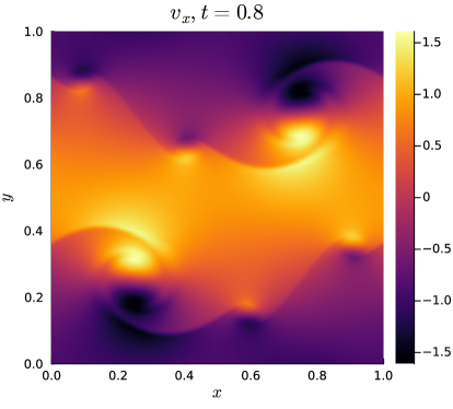
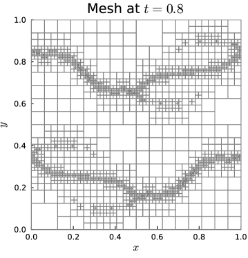
For this setup, a $p=3$ PERK scheme with $E=\{3,4,7\}$ stage evaluations is constructed, where the admissible timestep doubles for each family member. The mesh is allowed to change every $N_{\text{AMR}}=20$ timesteps, which involves the recomputation of the flagging-variables for the PERK integrator. In this case, the latter consumes $2.5\%$ of the total runtime with is the overhead due to the partitioning. Comparing this to the speedup of the stand-alone PERK scheme, this overhead is well invested additional computational effort. Comparing the simulation with $\text{P-ERK}_{3;\{3,4,7\}}$ to the standalone method $\text{P-ERK}_{3;7}$, the memory footprint increases in the mean by $20\%$.

The ratio of over ten runs averaged relative runtimes $\nicefrac{{\bar{\tau}}}{{\bar{\tau}_{\text{P-ERK}_{3;\{3,4,7\}}}}}$ of the different schemes are tabulated in Table 7. Also, we provide the degree of optimality $\kappa=\tau_{\text{Opt}}/\bar{\tau}$ cf. 6.9 and the number of performed scalar RHS evaluations $N_{\text{RHS}}^{\text{Actual}}$ 6.1 for the different schemes. For each method we compare to, the AMR interval is adjusted such that approximately the same number of grid refinements is performed as for the simulation with the PERK family. This is roughly equivalent to performing the mesh refinement at the same physical timestamps. When comparing the different schemes it is important to note that, while the simulations are equipped with identical parameters (except for CFL number and AMR interval $N_{\text{AMR}}$), the AMR indicator which governs local mesh refinement or coarsening is based on the solution itself, which is inevitably different for the different methods. This becomes already apparent for this example as the $\text{DGLDD}_{3;7}$ [76] scheme is slightly faster than the optimized $\text{P-ERK}_{3;7}$ scheme which can be traced back to the fact that the finest level is reached later for the simulation with the $\text{DGLDD}_{3;7}$ scheme, hence imposing the timestep restriction later.

Overall, the $\text{P-ERK}_{3;\{3,4,7\}}$ is the fastest method for this testcase with all other methods being at least $40\%$ slower. For this example we have a four times as large overall timestep for the $\text{P-ERK}_{3;\{3,4,7\}}$ scheme compared to the $\text{SSP}_{3;3}$ method while observing a speedup of factor $2.356$. Comparing this to the examples given in [2] where the authors observe speedups of about $4.3$ across examples for an eight times as large timestep (compared to the $\text{SSP}_{3;3}$) we conclude that we have essentially the same ratio of speedup per timestep increase.

The four-stage method $\text{CKLLS}_{3;4}$ [78] is not significantly faster than the canonical Shu-Osher ssp scheme, and is thus not considered in the following examples. This is possibly due to optimization for Navier-Stokes equations where diffusion plays a more dominant role than in the convection-dominated flows considered here.

Method	$\nicefrac{{\bar{\tau}}}{{\bar{\tau}_{\text{P-ERK}_{3;\{3,4,7\}}}}}$	$\nicefrac{{\tau_{\text{Opt}}}}{{\bar{\tau}}}$	$N_{\text{RHS}}^{\text{Actual}}$
$\text{P-ERK}_{3;\{3,4,7\}}$	$1.0$	$68.8\%$	$5.26\cdot 10^{9\hphantom{0}}$
$\text{P-ERK}_{3;7}$	$1.468$	$46.9\%$	$9.27\cdot 10^{9\hphantom{0}}$
$\text{SSP}_{3;3}$	$2.356$	$29.2\%$	$1.42\cdot 10^{10}$
$\text{DGLDD}_{3;7}$ [76]	$1.412$	$48.8\%$	$8.53\cdot 10^{9\hphantom{0}}$
$\text{PKD3S}_{3;5}$ [77]	$1.854$	$37.1\%$	$1.07\cdot 10^{10}$
$\text{RDPKFSAL}_{3;5}$ [79]	$2.171$	$31.7\%$	$1.30\cdot 10^{10}$
$\text{CKLLS}_{3;4}$ [78]	$2.350$	$29.3\%$	$1.45\cdot 10^{10}$

Table 7: Runtimes, optimality fraction 6.9, and number of scalar RHS evaluations 6.1 of different third-order ode solvers compared to the optimized $p=3,S=\{3,4,7\}$ PERK scheme for the periodic shear-layer.

7.1.2 Visco-Resistive Orszag-Tang Vortex

We consider the classic Orszag-Tang vortex [85] in the context of the vrMHD equations [86]. The ideal mhd equations are implemented with divergence cleaning through a GLM approach [87, 88] and extended by viscous and resistive terms by means of the BR1 scheme [80]

As in [86] the domain is $\Omega=[0,2\pi]^{2}$ and the gas parameters are set to $\gamma=\frac{5}{3}$, $\text{Pr}=1$. Compared to [86] we reduce viscosity and resistivity by one order of magnitude to $\mu=\nu=10^{-3}$ to stay convection-dominated (cf. (3.3)) even in the finest parts of the mesh. The initial condition is given by [86]

$$\boldsymbol{u}_{\text{primal}}(t_{0}=0,x,y)=\begin{pmatrix}\rho\\ v_{x}\\ v_{y}\\ v_{z}\\ p\\ B_{x}\\ B_{y}\\ B_{z}\end{pmatrix}=\begin{pmatrix}1.0\\ -2\sqrt{\pi}\sin(y)\\ 2\sqrt{\pi}\sin(x)\\ 0.0\\ \frac{15}{4}+\frac{1}{4}\cos(4x)+\frac{4}{5}\cos(2x)\cos(y)-\cos(x)\cos(y)+\frac{1}{4}\cos(2y)\\ -\sin(2y)\\ \sin(2x)\\ 0.0\end{pmatrix}$$ (7.2)

and the simulation is run until $t_{f}=2.0$ as in [86]. Note that in the vrMHD equations employed in [86] the magnetic terms are nondimensionalized using viscous and resistive Lundquist numbers, which is different from [87] used in this work. The grid cells vary between $h=\nicefrac{{2\pi}}{{2^{5}}}$ and $h=\nicefrac{{2\pi}}{{2^{9}}}$, i.e., a mesh with five consecutive levels of refinement is employed.

To discretize the spatial derivatives a split-form DG method [66] is used. The surface-flux itself is split up into conserved terms which are discretized using the Rusanov/Local Lax-Friedrichs flux and a non-conserved part for which a specialized flux is employed [89, 90]. Also for the volume flux/integral the conservative and non-conserved terms are treated differently. For this, we use the central flux for the conserved terms alongside the flux for the nonconservative Powell term [89]. As AMR indicator we employ the shock-capturing indicator developed in [68] based on density-pressure $\rho\cdot p$. This particular example benefits heavily from AMR since the configuration leads to initially sharp structures cf. Fig. 8 requiring accurate resolution which are then, due to the viscous effects, damped out over time with less need for high resolution.

(a) Pressure $p$ at $t=1.0$ for the visco-resistive Orszag-Tang vortex.

(b) Four times refined mesh at $t=1.0$.

Figure 8: Pressure $p$ at $t=1.0$ for the visco-resistive Orszag-Tang vortex (Fig. 8a) and corresponding adaptively refined mesh (Fig. 8b).

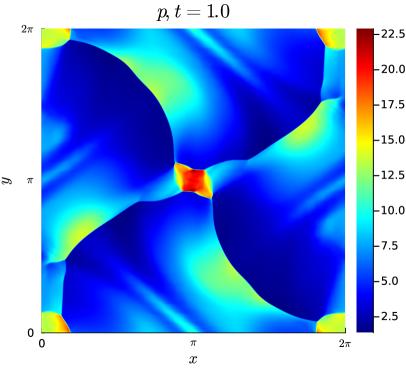
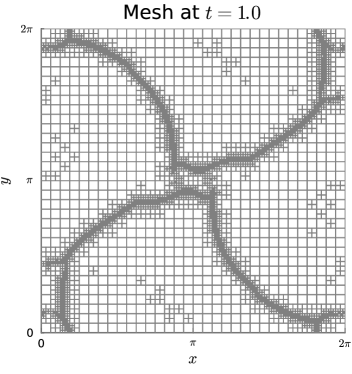
For time discretization, we employ the three-level $p=3,E=\{3,4,6\}$ optimized PERK family and compare it against the standalone $S=6$ PERK scheme, the $\text{SSP}_{3;3}$ method, $\text{DGLDD}_{3;7}$, and $\text{PKD3S}_{3;5}$ with runtimes provided in Table 8. As the ideal GLM-MHD equations require a CFL-based timestep for the divergence cleaning mechanism, we also supply a CFL number to $\text{RDPKFSAL}_{3;5}$ instead of an adaptive error-controlled timestep. As for the other cases, the PERK family is the fastest method among the considered ones. We observe that linear/absolute stability governs in this case the maximum admissible timestep as both the family as well as the standalone optimized PERK schemes outperform the other schemes. Furthermore, the $\text{SSP}_{3;3}$ scheme is the slowest Runge-Kutta method, which matches the expectations as this scheme is not optimized at all for a special class of semidiscretizations, in contrast to the other methods. As for the previous example, we obtain for a four times larger stable timestep for the $\text{P-ERK}_{3;\{3,4,6\}}$ scheme compared to the $\text{SSP}_{3;3}$ a speedup by a factor of $2.005$ which is again the same ratio of speedup per timestep increase demonstrated in the examples in [2].

Method	$\nicefrac{{\bar{\tau}}}{{\bar{\tau}_{\text{P-ERK}_{3;\{3,4,7\}}}}}$	$\nicefrac{{\tau_{\text{Opt}}}}{{\bar{\tau}}}$	$N_{\text{RHS}}^{\text{Actual}}$
$\text{P-ERK}_{3;\{3,4,6\}}$	$1.0$	$58.2\%$	$1.44\cdot 10^{10}$
$\text{P-ERK}_{3;6}$	$1.248$	$46.6\%$	$2.07\cdot 10^{10}$
$\text{SSP}_{3;3}$	$2.005$	$29.0\%$	$3.28\cdot 10^{10}$
$\text{DGLDD}_{3;7}$ [76]	$1.575$	$37.0\%$	$2.55\cdot 10^{10}$
$\text{PKD3S}_{3;5}$ [77]	$1.717$	$33.9\%$	$2.72\cdot 10^{10}$
$\text{RDPKFSAL}_{3;5}$ [79]	$1.649$	$35.3\%$	$2.72\cdot 10^{10}$

Table 8: Runtimes, optimality fraction 6.9, and number of scalar RHS evaluations 6.1 of different third-order integrators compared to the optimized $p=3,S=\{3,4,6\}$ PERK integrator for the visco-resistive Orszag-Tang vortex.

In terms of performance, there are $3.92\cdot 10^{9}$ excess scalar RHS evaluations which lead to an overall $1.718$ slower-than-optimal PERK scheme, i.e., for this case a significant speed-up would be possible if a full range of optimized methods without monotonicity violation could be employed. The update of the partition identifiers amounts to $1.0\%$ of the total runtime, that is, the overhead due to the partitioning is again negligible. The memory requirements of the $\text{P-ERK}_{3;\{3,4,6\}}$ scheme are on average $28\%$ larger than for the standalone $\text{P-ERK}_{3;6}$ scheme.

7.1.3 3D Taylor-Green Vortex

The three-dimensional Taylor-Green vortex is a well-known reference problem showcasing emerging turbulence from a simple initial condition which is followed by the decay of the turbulent structures accompanied by kinetic energy dissipation [91, 92]. The initial condition in primitive variables is given by

$$\boldsymbol{u}_{\text{prim}}(t_{0}=0,x,y,z)=\begin{pmatrix}\rho\\ v_{x}\\ v_{y}\\ v_{z}\\ p\end{pmatrix}=\begin{pmatrix}1\\ \sin(x)\cos(y)\cos(z)\\ -\cos(x)\sin(y)\cos(z)\\ 0\\ p_{0}+\frac{1}{16}\rho\Big{(}\big{(}\cos(2x)+\cos(2y)\big{)}\big{(}2+\cos(2z)\big{)}\Big{)}\end{pmatrix},$$ (7.3)

where $p_{0}=\frac{\rho}{M^{2}\gamma}$ with Mach number $M=0.1$ as in [93]. The Prandtl and Reynolds number are $\text{Pr}=0.72$ and $\text{Re}=1600$, and the compressible Navier-Stokes equations are simulated on $\Omega=[0,2\pi]^{3}$ equipped with periodic boundaries until $t_{f}=20.0$.

In terms of spatial discretization, we employ solution polynomials of degree $k=2$, HLLE surface flux [67], and an entropy-conservative volume flux [70, 66]. We employ a simple AMR indicator based on the enstrophy

$$\epsilon\coloneqq 0.5\,\rho\,\boldsymbol{\omega}\cdot\boldsymbol{\omega}\,,$$ (7.4)

which refines cells once a specified threshold is exceeded. Doing so, we expect the mesh to be refined in regions where the vorticity $\boldsymbol{\omega}\coloneqq\nabla\times\boldsymbol{v}$ is high, i.e., where turbulent structures are emerging. The initial condition is discretized using $16^{3}$ cells which are allowed to be two times refined corresponding to a smallest cell size of $h=\frac{2\pi}{64}$. While the Taylor-Green vortex is certainly not a classic use case for AMR it allows us to examine the cost of the dynamic re-assignment of cells to partitions for a three-dimensional problem.

In terms of the temporal integrators, we employ the three-level $p=3,E=\{3,4,6\}$ optimized PERK family and compare it against the standalone $S=6$ PERK scheme, the $\text{SSP}_{3;3}$ method, $\text{DGLDD}_{3;7}$ [76], $\text{PKD3S}_{3;5}$ [77], and $\text{RDPKFSAL}_{3;5}$ [79] with runtimes provided in Table 9. The integrated enstrophy

$$\bar{\epsilon}\coloneqq\frac{1}{\rho_{0}|\Omega|}\int_{\Omega}\epsilon\,\text{d}\Omega$$ (7.5)

and integrated kinetic energy

$$\overline{E}_{\text{kin}}=\frac{1}{\rho_{0}|\Omega|}\int_{\Omega}\frac{1}{2}\rho\boldsymbol{v}\cdot\boldsymbol{v}\,\text{d}\Omega$$ (7.6)

showcase for the Taylor-Green vortex a characteristic behavior which allows for a meaningful comparsion of different simulations. These are plotted in Fig. 9 for the simulation with the $\text{P-ERK}_{3;\{3,4,6\}}$ scheme and compared against the fourth-order finite difference method from [93] on uniform $64^{3},128^{3}$ grids and a reference solution from [54] obtained by a dealiased pseudo-spectral method with $512^{3}$ grid cells. Despite the relatively coarse grid involving cells of size $h=\frac{2\pi}{16}$ the simulation using the dgsem method captures the increase in enstrophy better than the fourth-order finite difference method on a uniform $64^{3}$ grid, see Fig. 9a. Similarly, the decay of the integrated kinetic energy is also captured very well by the dgsem method on an adaptively refined grid with partitioned time integration, cf. Fig. 9b.

(a) Integrated enstrophy $\bar{\epsilon}$ (7.5) for the 3D Taylor-Green vortex.

(b) Integrated kinetic energy $\overline{E}_{\text{kin}}$ (7.6) for the 3D Taylor-Green vortex.

Figure 9: Integrated enstrophy $\bar{\epsilon}$ (7.5) (Fig. 9a) and integrated kinetic energy $\overline{E}_{\text{kin}}$ (7.6) (Fig. 9b) for the 3D Taylor-Green vortex with AMR (blue). For the simulation with AMR the spatial resolution varies from $h=\frac{2\pi}{16}$ to $h=\frac{2\pi}{64}$.

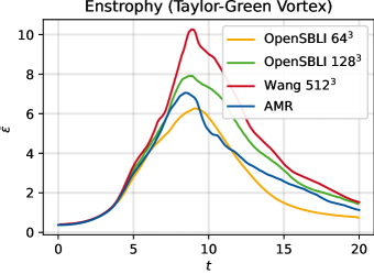
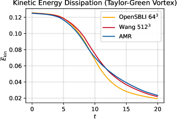
When comparing the runtimes of the different schemes in Table 9 we observe that the $\text{P-ERK}_{3;\{3,4,6\}}$ scheme is again the fastest method among the considered ones, although the standalone $S=6$ PERK scheme is only about $4\%$ slower. This is not surprising, as for the majority of timesteps most cells are completely refined and thus only very little speed-up may be gained. This is also reflected by the speedup that could be gained from a hypothetical ideally scaling set of methods. The $5.44\cdot 10^{9}$ excess scalar RHS evaluations lead only to an overall $1.034$ slower-than-optimal PERK scheme. We included this example for instructive purposes since it showcases that also (at least for small) 3D problems the overhead of the re-computation of the partitioning datastructures does not exceed speedup gained. In particular, only $0.3\%$ of the total runtime is spent on the constuction of the flagging variables after mesh changes. In this case, the memory footprint of the $\text{P-ERK}_{3;\{3,4,6\}}$ scheme is on average only $7\%$ larger than the standalone $\text{P-ERK}_{3;6}$ scheme.

Method	$\nicefrac{{\bar{\tau}}}{{\bar{\tau}_{\text{P-ERK}_{3;\{3,4,7\}}}}}$	$\nicefrac{{\tau_{\text{Opt}}}}{{\bar{\tau}}}$	$N_{\text{RHS}}^{\text{Actual}}$
$\text{P-ERK}_{3;\{3,4,6\}}$	$1.0$	$96.8\%$
$\text{P-ERK}_{3;6}$	$1.068$	$90.6\%$
$\text{SSP}_{3;3}$	$1.768$	$54.7\%$
$\text{DGLDD}_{3;7}$ [76]	$1.250$	$77.4\%$
$\text{PKD3S}_{3;5}$ [77]	$1.622$	$59.7\%$
$\text{RDPKFSAL}_{3;5}$ [79]	$1.425$	$67.9\%$

Table 9: Runtimes, optimality fraction 6.9, and number of scalar RHS evaluations 6.1 of different third-order integrators compared to the optimized $p=3,S=\{3,4,6\}$ PERK integrator for the Taylor-Green vortex.

7.2 Hyperbolic Equations

In addition to the isentropic vortex test case used for verification in Section 5 we present additional applications to inviscid, hyperbolic problems. In particular, this is the first time the PERK schemes are applied to invsicid problems, apart from the isentropic vortex used in convergence tests. For inviscid problems the issues concerning nonlinear stability discussed in Section 3.2 resurface and a simulation with three-level ($R=3$) PERK schemes demands in general a reduction of the timestep compared te the optimized standalone scheme. Recall that for hyperbolic-parabolic problems the CFL number did not have to be reduced for simulations with PERK schemes compared to the standalone scheme. This clearly impairs the performance of the PERK schemes for inviscid problems and correspondingly, we do not see the same speedup as for the viscous problems.

7.2.1 Kelvin-Helmholtz Instability

The inviscid Kelvin-Helmholtz instability is a suitable testcase for the AMR-based dynamic ode partitioning developed in this work. The initial condition can be accurately represented with a quite coarse discretization while the emerging instability requires a significantly finer resolution. We use the setup from [62] where the initial condition is given by

$$\boldsymbol{u}_{\text{primal}}(t_{0}=0,x,y)=\begin{pmatrix}\rho\\ v_{x}\\ v_{y}\\ p\end{pmatrix}=\begin{pmatrix}0.5+0.75B(y)\\ 0.5\big{(}B(y)-1\big{)}\\ 0.1\sin(2\pi x)\\ 1\end{pmatrix}$$ (7.7)

with $B(y)=\tanh(15y+7.5)-\tanh(15y-7.5)$ which corresponds to Mach number $\text{Ma}\leq 0.6$. The compressible Euler equations are discretized using the dgsem with $k=3$ local polynomials, hlle surface-flux [67], subcell shock-capturing [68] to avoid spurious oscillations and entropy-conserving volume flux [70, 69]. Initially, the domain $\Omega=[-1,1]^{2}$ is discretized with $2^{4}\times 2^{4}$ cells which are allowed to be refined five times, i.e., the finest cells may have edge length $h=2^{-8}$. The indicator for AMR coincides in this case with the shock-capturing indicator [68] and is based on the density $\rho$. For time-integration, the $p=3,E=\{4,6,11\}$ PERK family is employed where the admissible timestep doubles with increasing stage evaluations $E$. In contrast to the viscous flows from the previous section, the CFL number of the $\text{P-ERK}_{3;\{4,6,11\}}$ scheme has to be reduced to $70\%$ of the CFL number of the $\text{P-ERK}_{3;11}$ scheme. This reduction is a consequence of the troubling nonlinear stability properties of the PERK schemes at scheme boundaries, cf. Section 3.2.

The computational mesh and solution at final time $t_{f}=3.0$ are displayed in Fig. 10.

(a) Density $\rho$ at final time $t_{f}=3.0$ for the Kelvin-Helmholtz instability.

(b) Five times refined mesh at $t_{f}=3.0$.

Figure 10: Density $\rho$ at final time $t_{f}=3.0$ for the Kelvin-Helmholtz instability 7.7 (Fig. 10a) and corresponding adaptively refined mesh Fig. 10b.

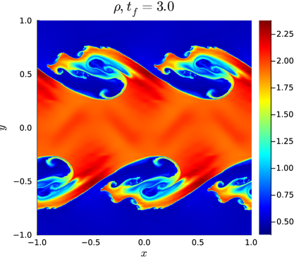
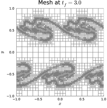
As for the viscous problems, we compare the PERK family to the stand-alone $p=3,S=11$ scheme and the $\text{SSP}_{3;3}$, $\text{DGLDD}_{3;7}$, $\text{PKD3S}_{3;5}$, and $\text{RDPKFSAL}_{3;5}$ schemes. The AMR-interval $N_{\text{AMR}}$ (cf. (6.2)) is adjusted according to the timesteps undertaken by the different methods to have an approximately equal AMR load. The runtimes $\tau$ are averaged over ten runs on a shared-memory multicore thread-parallelized machine and presented in Table 10. The $\text{P-ERK}_{3;\{4,6,11\}}$ is in this case the most efficient integrator with minimal runtime. Notably, the $\text{DGLDD}_{3;7}$ method is only slightly slower and even faster than the optimized $\text{P-ERK}_{3;11}$ scheme. This is attributed to favorable nonlinear stability properties (low-dispersion, low-dissipation), which are for this example (and for the inviscid problems in this section overall) more relevant than optimized absolute stability. Similarly, the $\text{SSP}_{3;3}$ scheme performs also better than the $\text{PKD3S}_{3;5}$ and $\text{RDPKFSAL}_{3;5}$ schemes despite that these are optimized for DG methods and computational fluid dynamics, respectively. Note that this was not the case for the previous hyperbolic-parabolic examples, i.e., the $\text{SSP}_{3;3}$ scheme did not outperform any of the optimized schemes for viscous problems.

Method	$\nicefrac{{\bar{\tau}}}{{\bar{\tau}_{\text{P-ERK}_{3;\{3,4,7\}}}}}$	$\nicefrac{{\tau_{\text{Opt}}}}{{\bar{\tau}}}$	$N_{\text{RHS}}^{\text{Actual}}$
$\text{P-ERK}_{3;\{4,6,11\}}$	$1.0$	$92.4\%$	$3.78\cdot 10^{9}$
$\text{P-ERK}_{3;11}$	$1.311$	$70.5\%$	$5.30\cdot 10^{9}$
$\text{SSP}_{3;3}$	$1.426$	$64.8\%$	$6.62\cdot 10^{9}$
$\text{DGLDD}_{3;7}$ [76]	$1.169$	$79.1\%$	$5.19\cdot 10^{9}$
$\text{PKD3S}_{3;5}$ [77]	$1.866$	$49.4\%$	$8.36\cdot 10^{9}$
$\text{RDPKFSAL}_{3;5}$ [79]	$1.659$	$55.7\%$	$6.54\cdot 10^{9}$

Table 10: Runtimes, optimality fraction 6.9, and number of scalar RHS evaluations 6.1 of different third-order integrators compared to the optimized $p=3,S=\{4,6,11\}$ PERK integrator for the inviscid Kelvin-Helmholtz instability.

The update of the identifier variables required for the partitioning amounts in this case to about $0.4\%$ of the total runtime $\tau_{\text{P-ERK}}$. The memory footprint of the $\text{P-ERK}_{3;\{4,6,11\}}$ scheme is on average $23\%$ larger than the standalone $\text{P-ERK}_{3;11}$ scheme. To assess the optimality, or, in other words, the room for further improvements of using, e.g., a PERK family with more members and higher stages, we compute the excess scalar RHS evaluations according to (6.2). For this example, there are $3.80\cdot 10^{8}$ additional scalar RHS evaluations per conserved variable which increase the runtime of the employed $\text{P-ERK}_{3;\{4,6,11\}}$ scheme to $1.035$ of the optimal one, neglecting overhead due to additional levels. This value results from the fact that the vast majority of the cells is distributed among the finest three levels. In particular, at final time $t_{f}=3.0$ the three non-optimal integrated levels form only $6\%$ of the entire number of cells, cf. Fig. 10b. In other words, the majority of the cells are integrated optimally with results in a speed-up of $30\%$ compared to the standalone $\text{P-ERK}_{3;11}$ scheme.

When comparing the number of performed scalar RHS evaluations $N_{\text{RHS}}^{\text{Actual}}$ to the runtime $\tau$ we observe not exactly a linear correspondence. This is due to two factors: First, the AMR contributes a fixed-cost to the overall measured runtime $\tau$ which does not decrease with the number of scalar RHS evaluations. Second, and more signficantly, the employed shock-capturing mechanism [68] leads to different computational costs for different cells, as for some a plain dgsem reconstruction is employed while for others a blending of dgsem and subcell Finite Volume reconstruction is necessary. The influence of this can clearly be seen by comparing the runtimes of the standalone $\text{P-ERK}_{3;11}$ scheme and the $\text{DGLDD}_{3;7}$ scheme which have roughly the same number of scalar RHS evaluations. The $\text{DGLDD}_{3;7}$ scheme is, however, over-proportionally faster than the $\text{P-ERK}_{3;11}$ scheme, which is attributed to the lower computational cost of the employed shock-capturing mechanism. Similarly, the speedup of the $\text{P-ERK}_{3;\{4,6,11\}}$ scheme compared to the $\text{P-ERK}_{3;11}$ scheme is not exactly proportional to the number of scalar RHS evaluations, again due to increased computational cost of the employed shock-capturing mechanism. This can be seen as a price of the poor nonlinear stability properties of the PERK schemes which cause more cells to rely on a blend of dgsem and subcell Finite Volume reconstruction.

7.2.2 Rayleigh-Taylor Instability

Another classic example is the Rayleigh-Taylor instability, where a heavier fluid gets pushed into a lighter one, leading to complicated flow structures beneath the characteristic mushroom cap. The configuration follows [94] with reflective boundary conditions on the boundaries in $x$-direction and weakly enforced Dirichlet boundary conditions in $y$-direction. The domain $\Omega=[0,0.25]\times[0,1]$ is initially discretized with $N_{x}=12,N_{y}=4\cdot N_{x}=48$ third-order ($k=3$) elements. The spatial discretization is analogous to the Kelvin-Helmholtz instability from Section 7.2.1 and the simulation is run up to $t_{f}=1.95$ as in [94]. Following [94], we set the ratio of specific heats $\gamma=\nicefrac{{5}}{{3}}$ and the initial state to

$$\boldsymbol{u}_{\text{prim}}(t_{0}=0,x,y)=\begin{pmatrix}\rho\\ v_{x}\\ v_{y}\\ p\end{pmatrix}=\begin{pmatrix}\begin{cases}2.0&y\leq 0.5\\ 1.0&y>0.5\end{cases}\\ 0.0\\ ck\cos(8\pi x)\\ \begin{cases}2.0\cdot y+1.0&y\leq 0.5\\ y+1.5&y>0.5\end{cases}\end{pmatrix}$$ (7.8)

where $c=\sqrt{\frac{\gamma p}{\rho}}$ denotes the speed of sound and $k=-0.025$ quantifies the strength of the initial perturbation.

Each cell is allowed to be refined at most six times, i.e., the theoretically maximum resolution is $768\times 3072$ with $h=\nicefrac{{1}}{{3072}}$. For time integration we employ a $p=3,E=\{3,4,6\}$ scheme where the maximum admissible timestep doubles for each family member. Thus, the finest three levels can be integrated optimally and only the remaining levels are not efficiently integrated. Compared to the standalone $\text{P-ERK}_{3;6}$ scheme the CFL number of the $\text{P-ERK}_{3;\{3,4,6\}}$ is reduced to $96\%$ of the optimal value. We observe, however, that the $\text{P-ERK}_{3;4}$ has a higher stage-normalized CFL number $\text{CFL}/E$, rendering it more efficient. Consequently, we employ $\text{P-ERK}_{3;4}$ for the runtime comparisons in Table 11. The computation of the partitioning variables consumes about $4.4\%$ of the total runtime. This increase compared to the other examples is due to the usage of the in principle unstructured p4est mesh which requires the computation of the minimum edge length for each cell. This is additional effort compared to the necessarily square/cubic cells forming the TreeMesh, where each cells’ characteristic length is fully determined by the position of the associated node in the underlying tree datastructure. In terms of additional memory consumption, the $\text{P-ERK}_{3;\{3,4,6\}}$ scheme requires on average $34\%$ more memory than the standalone $\text{P-ERK}_{3;4}$ scheme.

(a) Density $\rho$ at final time $t_{f}=1.95$ for the Rayleigh-Taylor instability.

(b) Five times refined mesh at $t_{f}=1.95$.

Figure 11: Density $\rho$ at final time $t_{f}=1.95$ for the Rayleigh-Taylor instability 7.8 (Fig. 11a) and corresponding adaptively refined mesh Fig. 11b.

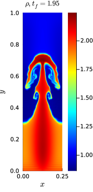
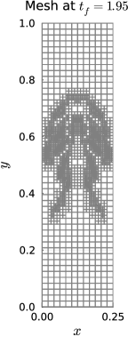
As for the Kelvin-Helmholtz instability, the $\text{P-ERK}_{3;\{3,4,6\}}$ scheme is the fastest method among the considered ones, see Table 11 followed by the standalone optimized $\text{P-ERK}_{3;4}$ scheme. Notably, the usually well-performing $\text{DGLDD}_{3;7}$ [76] scheme is in this case relatively slow. As for the Kelvin-Helmholtz instability, we observe a discrepancy between the number of scalar RHS evaluations $N_{\text{RHS}}^{\text{Actual}}$ and the runtime $\tau$. For instance, the $\text{P-ERK}_{3;\{3,4,6\}}$ scheme has roughly half the number of scalar RHS evaluations of the $\text{PKD3S}_{3;5}$ scheme. However, the $\text{P-ERK}_{3;\{3,4,6\}}$ scheme is only about $1.4$ times faster than the $\text{PKD3S}_{3;5}$ scheme. This is attributed to more cells relying on the expensive subcell shock-capturing mechanism [68] for the $\text{P-ERK}_{3;\{3,4,6\}}$ scheme than for the $\text{PKD3S}_{3;5}$ scheme. Additionally, the AMR fixed-costs which are for the $\text{P-ERK}_{3;\{3,4,6\}}$ scheme about $23\%$ of the total runtime, do not decrease if $N_{\text{RHS}}^{\text{Actual}}$ is reduced.

Method	$\nicefrac{{\bar{\tau}}}{{\bar{\tau}_{\text{P-ERK}_{3;\{3,4,7\}}}}}$	$\nicefrac{{\tau_{\text{Opt}}}}{{\bar{\tau}}}$	$N_{\text{RHS}}^{\text{Actual}}$
$\text{P-ERK}_{3;\{3,4,6\}}$	$1.0$	$82.5\%$	$1.25\cdot 10^{10}$
$\text{P-ERK}_{3;4}$	$1.126$	$73.3\%$	$1.84\cdot 10^{10}$
$\text{SSP}_{3;3}$	$1.205$	$68.5\%$	$2.04\cdot 10^{10}$
$\text{DGLDD}_{3;7}$ [76]	$1.751$	$47.1\%$	$3.32\cdot 10^{10}$
$\text{PKD3S}_{3;5}$ [77]	$1.402$	$58.9\%$	$2.40\cdot 10^{10}$
$\text{RDPKFSAL}_{3;5}$ [79]	$1.292$	$63.9\%$	$1.44\cdot 10^{10}$

Table 11: Runtimes, optimality fraction 6.9, and number of scalar RHS evaluations 6.1 of different third-order integrators compared to the optimized $p=3,S=\{3,4,6\}$ PERK integrator for the inviscid Rayleigh-Taylor instability.

7.2.3 MHD Rotor

In order to go beyond the Euler equations of gas dynamics we consider the ideal mhd equations with divergence cleaning through a GLM approach [87, 88]. A classic testcase thereof is the mhd rotor [95] which we also study here. The somewhat lenghty initial condition is provided in B.

In terms of spatial discretization, we employ $k=4$ local polynomials with the fluxes being discretized analogous to the inviscid fluxes from the visco-resistive Orszag-Tang vortex studied in Section 7.1.2. Again, for AMR indication the shock-capturing mechanism from [68] based on density-pressure $\rho\cdot p$ is employed. The pressure distribution at final time $t_{f}=0.15$ is displayed in Fig. 12 together with the corresponding mesh.

(a) Pressure $p$ at final time $t_{f}=0.15$ for the ideal MHD rotor.

(b) Six times refined mesh at $t_{f}=0.15$.

Figure 12: Pressure $p$ at final time $t_{f}=0.15$ for the MHD rotor [95] (Fig. 12a) and corresponding adaptively refined mesh Fig. 12b.

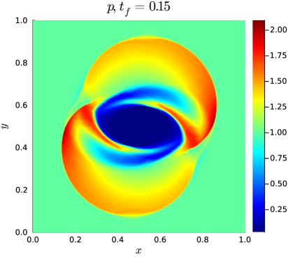
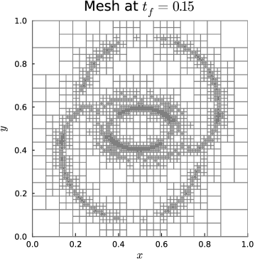
For this example the $p=3$, $E=\{4,6,10\}$ scheme is a suitable choice for the PERK family where the maximum admissible timestep doubles for each family member. Similar to the Rayleigh-Taylor instability, the CFL number of the $\text{P-ERK}_{3;\{4,6,10\}}$ scheme has not to be significantly reduced compared to the standalone $\text{P-ERK}_{3;10}$ scheme. We compare the PERK family to the best performing stand-alone $\text{P-ERK}_{3;6}$ optimized method, $\text{SSP}_{3;3}$, $\text{DGLDD}_{3;7}$, $\text{PKD3S}_{3;5}$, and $\text{RDPKFSAL}_{3;5}$ (with CFL-determined timestep). The results are tabulated in Table 12. As for the previous examples, the PERK family is the fastest method among the considered ones with the standalone $S=6$ PERK scheme being about $10\%$ slower. The runtimes for the $\text{PKD3S}_{3;5}$ and $\text{RDPKFSAL}_{3;5}$ scheme are almost identical which is not surprising since the scheme $\text{RDPKFSAL}_{3;5}$ developed in [79] is based on the $\text{PKD3S}_{3;5}$ scheme [77].

Method	$\nicefrac{{\bar{\tau}}}{{\bar{\tau}_{\text{P-ERK}_{3;\{3,4,7\}}}}}$	$\nicefrac{{\tau_{\text{Opt}}}}{{\bar{\tau}}}$	$N_{\text{RHS}}^{\text{Actual}}$
$\text{P-ERK}_{3;\{4,6,10\}}$	$1.0$	$88.1\%$	$2.35\cdot 10^{9}$
$\text{P-ERK}_{3;6}$	$1.097$	$80.6\%$	$3.23\cdot 10^{9}$
$\text{SSP}_{3;3}$	$1.492$	$57.9\%$	$4.43\cdot 10^{9}$
$\text{DGLDD}_{3;7}$ [76]	$1.148$	$76.7\%$	$3.51\cdot 10^{9}$
$\text{PKD3S}_{3;5}$ [77]	$1.195$	$73.7\%$	$3.56\cdot 10^{9}$
$\text{RDPKFSAL}_{3;5}$ [79]	$1.192$	$73.9\%$	$3.56\cdot 10^{9}$

Table 12: Runtimes, optimality fraction 6.9, and number of scalar RHS evaluations 6.1 of different third-order integrators compared to the optimized $p=3,S=\{4,6,10\}$ PERK integrator for the ideal MHD rotor.

For this case, a fully optimal PERK scheme could save $7.71\cdot 10^{7}$ scalar RHS calls per field. Correspondingly, the here employed three-level PERK scheme is $1.135$ times slower than a hypothetical optimal PERK family, again neglecting potential overhead due to the usage of additional levels. The dynamic updating of the partitioning indicator variables amounts in this case to $0.8\%$ of the total runtime. The memory footprint of the $\text{P-ERK}_{3;\{4,6,10\}}$ scheme is on average $11\%$ larger than the standalone $\text{P-ERK}_{3;6}$ scheme. As for the other two inviscid examples, the decrease in runtime $\tau$ of the PERK schemes is not proportional to the number of scalar RHS evaluations $N_{\text{RHS}}^{\text{Actual}}$. The reason behind this is that for the $\text{P-ERK}_{3;\{4,6,10\}}$ scheme a larger number of cells require the subcell stabilizing mechanism [68] compared to the standalone schemes. This is due to the poor nonlinear stability properties of the PERK schemes and thus an increased computational cost per RHS evaluation.

8 Conclusions

In this work, we applied the Paired-Explicit Runge-Kutta (P-ERK) schemes by Vermeire et. al. [1, 2] to convection-dominated, compressible flows with adaptive mesh refinement. For a range of hyperbolic and hyperbolic-parabolic examples we demonstrate speed-up compared to state-of-the-art optimized Runge-Kutta methods. In particular, the PERK outperform for every considered case the non-multirate schemes by factors up to $2.4$ for viscous problems and $1.8$ for inviscid problems.

Additional data structures are required for the partitioning, which can for all considered examples be set up in less of $5\%$ of the total runtime. The memory footprint of partitioning variables leads to $7-34\%$ additional memory consumption compared to the standalone schemes. For the shown applications a public reproducibility repository is provided [24].

In general, the PERK schemes perform better for PDE involving viscous fluxes compared to purely inviscid problems. This is due to the fact that the PERK schemes are in general not monotonicity-preserving and thus require the stabilizing shock-capturing strategy [68] on a larger number of cells than the standalone schemes. We investigated the mechanism behind this behaviour by conducting a thorough nonlinear stability analysis of the fully discrete, partitioned system. In particular, we show that the usage of the PERK schemes leads in general to a loss of the monotonicity properties of the spatial discretization. More precise, the monotonicity properties are violated at the intersection of different schemes, i.e., where the partitioning is performed. This restricts the PERK schemes to configurations with limited difference in stage evaluations among partitions for an efficient time integration.

Future work will focus on the constuction of fourth-order consistent PERK schemes and the application to unstructured meshes with adaptive mesh refinement.

Data Availability

All data generated or analyzed during this study are included in this published article and its supplementary information files.

Code Availability & Reproducibility

We provide a reproducibility repository [24] containing the source code and scripts and data to reproduce the results from Section 5 and Section 7.

Declaration of competing interest

The authors declare the following financial interests/personal relationships which may be considered as potential competing interests: Daniel Doehring financial support was provided by German Research Foundation.

CRediT authorship contribution statement

Daniel Doehring: Formal analysis, Investigation, Methodology, Software, Writing - original draft.
Michael Schlottke-Lakemper: Conceptualization, Software, Funding acquisition, Writing - review & editing.
Gregor J. Gassner: Conceptualization, Funding acquisition, Writing - review & editing.
Manuel Torrilhon: Conceptualization, Funding acquisition, Supervision, Writing - review & editing.

Appendix A P-ERK Schemes on a Smoothly Refined, High-Resolution Mesh

In order to give further evidence for the nonlinear stability analysis conducted in Section 3.2, we present a testcase where the PERK schemes are applied to a smooth, high-resolution mesh. The refinement factor $\alpha$ of neighboring cells is for this example close to $1$, i.e., the discontinuities in the mesh are substantially less pronounced than for the quad/octree-based AMR meshes. To this end, we construct a structured curved mesh by defining the mapping of the edges of the cartesian square $(\xi,\eta)\in[-1,1]^{2}$ onto curved edges $\boldsymbol{e}_{i},i=1,\dots,4$ of the computational domain. In particular, we employ the mapping

$$\boldsymbol{e}_{1}(\xi,\eta) =\begin{pmatrix}r_{0}+0.5(r_{1}-r_{0})(\xi+1)\\ 0\end{pmatrix}$$ (A.1a)

$$\boldsymbol{e}_{2}(\xi,\eta) =\begin{pmatrix}r_{1}\cos\big{(}0.5\pi(\eta+1)\big{)}\\ r_{1}\sin\big{(}0.5\pi(\eta+1)\big{)}\end{pmatrix}$$ (A.1b)

$$\boldsymbol{e}_{3}(\xi,\eta) =\begin{pmatrix}-r_{0}-0.5(r_{1}-r_{0})(\xi+1)\\ 0\end{pmatrix}$$ (A.1c)

$$\boldsymbol{e}_{4}(\xi,\eta) =\begin{pmatrix}r_{0}\cos\big{(}0.5\pi(\eta+1)\big{)}\\ r_{0}\sin\big{(}0.5\pi(\eta+1)\big{)}\end{pmatrix}$$ (A.1d)

where the edges $\boldsymbol{e}_{i}$ of the $[-1,1]^{2}$ cube are labeled counter-clockwise starting from the bottom $(\xi,\eta=0)$ edge. This mapping corresponds to a half-circle with radius $r_{1}$ from which a half-circle with radius $r_{0}$ is subtracted. The mesh is discretized using $N_{\xi}=192\times N_{\eta}=128$ cells and is displayed in Fig. 13.

Figure 13: High-resolution, structured mesh for demonstration of working PERK schemes on smooth meshes.

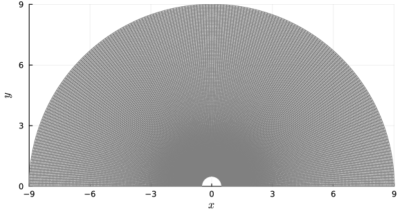
For this testcase we simulate the inviscid Euler equations of gas dynamics with $\gamma=1.4$ with initial condition

$$\boldsymbol{u}_{\text{prim}}(t_{0}=0,x,y)=\begin{pmatrix}\rho\\ v_{x}\\ v_{y}\\ p\end{pmatrix}=\begin{pmatrix}1.0\\ 0.0\\ 0.0\\ 1.0+2^{-\frac{(x-0.6r_{1})^{2}+y^{2}}{0.45^{2}}}\end{pmatrix}$$ (A.2)

which corresponds to a pressure perturbation with magnitude $p_{\text{max}}=2$ located at the right-bottom of the half-circle, cf. Fig. 14a.

In terms of spatial discretization we employ the dgsem with $k=2$ local polynomials, hll surface-flux and an entropy-conservative volume flux [70, 66] with reflective boundaires. In particular, no techniques like shock capturing or positivity-preserving limiters are employed to suppress spurious oscillations.

For time-integration, second-order accurate stability polynomials with degrees $S=\allowbreak\{4,\allowbreak 6,\allowbreak 8,\allowbreak\dots,\allowbreak 16\}$ are optimized, based on which we construct a range of PERK schemes. The gridcells are sorted into $R$ (number of PERK family members) bins based on their minimum edge length which govern the associated Runge-Kutta method. We test all combinations of PERK schemes with $E^{(1)}=4$ minimum stage evaluations, i.e., from the standalone $S=4$ scheme up to the $S=16,E=\{4,6,8,\dots,16\}$ family. For all combinations, the maximum admissible timestep is increased according to highest number of stage evaluations $E^{(R)}$. For this setup, across different PERK schemes, the stage-evaluation normalized CFL-number for stable simulation is essentially constant across PERK families, as shown in Table 13. For the sake of completeness we also provide the speedup compared to the Shu-Osher $p=3,S=3$ scheme, the reference method from [1, 2] in Table 13.

$E^{(R)}$	4	6	8	10	12	14	16
$\text{CFL}\cdot\frac{E^{(1)}}{E^{(R)}}$	$0.95$	$0.97$	$0.97$	$0.94$	$0.94$	$0.94$	$0.93$
$\frac{\tau_{\text{SSP}_{3;3}}}{\tau_{\text{P-ERK}_{2;4,\dots,E^{(R)}}}}$	$1.26$	$1.64$	$1.90$	$2.06$	$2.22$	$2.37$	$2.45$

Table 13: Normalized CFL numbers and speedup across different PERK schemes for the structured mesh testcase. Here, $E^{(1)}=4$ is the base scheme utilized in all cases.

For illustration, the final pressure distribution $p$ at $t_{f}=5.0$ is displayed in Fig. 14 alongside the initial perturbation according to (A.2).

(a) Initial pressure perturbation according to A.2.

(b) Pressure $p$ at final time $t_{f}=5.0$.

Figure 14: Initial pressure perturbation according to A.2 (Fig. 14a) and pressure $p$ at final time $t_{f}=5.0$ (Fig. 14b).

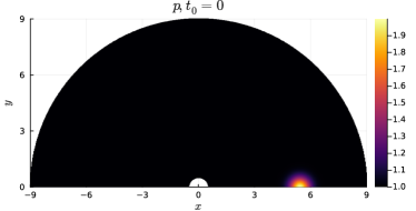
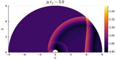
We repeated this testcase for a significantly coarser mesh with $N_{\xi}=48\times N_{\eta}=32$ cells and obtained qualitatively similar results. In particular, the normalized CFL number is again of similar value, with the largest value $\text{CFL}=1.04$ for the PERK scheme with $E^{(R)}=10$ and smallest value for $E^{(R)}=16$ with $\text{CFL}=0.95$.

This example demonstrates that the PERK schemes are a suitable multirate scheme, even for inviscid problems without stabilization. In particular, due to the smooth meshes, the discontinuity in the mesh is effectively eliminated and does not coincide with the discontinuity in the time integration method. This is the main difference to quad/octree-basedAMR meshes where the discontinuity in the mesh coincides with the discontinuity in the time integration method. In this case, the mesh refinement factor is always $\alpha=2$ and the difference in stage evaluations scales quadratically with the number of levels, leading to a discontinuity in methods for the finest levels.

Appendix B Ideal MHD Rotor: Initial Condition

For the simulation of the ideal MHD rotor we employ the initial condition from [95]. The radius $r_{0}$ of the spinning cylinder is set to $r_{0}=0.1$ while the medium is initially at rest for $r\geq r_{1}=0.115$ with radius $r(x,y)=\sqrt{(x-0.5)^{2}+(y-0.5)^{2}}$. The magnetic field is set uniformly to $\boldsymbol{B}(t_{0}=0,x,y)=\begin{pmatrix}\frac{5}{2\sqrt{\pi}}&0&0\end{pmatrix}$ as well as pressure $p(0,x,y)=1$ and $v_{z}(0,x,y)=0$. Inside the spinning cylinder, i.e., $r\leq r_{0}$ we set the density to $\rho(0,x,y)=10$ and the velocities to $v_{x}(0,x,y)=-20(y-0.5)$, $v_{y}(0,x,y)=20(x-0.5)$. In the transition from $r_{0}$ to $r_{1}$ we set the density to $\rho(0,x,y)=1+9f\big{(}r(x,y)\big{)}$ and the velocities to $v_{x}(0,x,y)=-20(y-0.5)f\big{(}r(x,y)\big{)}$, $v_{y}(0,x,y)=20(x-0.5)f\big{(}r(x,y)\big{)}$ with $f\big{(}r(x,y)\big{)}\coloneqq\frac{r_{1}-r(x,y)}{r_{1}}$. Outside of $r_{1}$, i.e., $r>r_{1}$ the medium is at rest $v_{x}(t_{0},x,y)=0$, $v_{y}(t_{0},x,y)=0$ and density is set to $\rho(0,x,y)=1$.

References

- Vermeire [2019] B. C. Vermeire, Paired explicit Runge-Kutta schemes for stiff systems of equations, Journal of Computational Physics 393 (2019) 465–483. doi:10.1016/j.jcp.2019.05.014.
- Nasab and Vermeire [2022] S. H. Nasab, B. C. Vermeire, Third-order paired explicit Runge-Kutta schemes for stiff systems of equations, Journal of Computational Physics 468 (2022) 111470. doi:10.1016/j.jcp.2022.111470.
- Godlewski and Raviart [2013] E. Godlewski, P.-A. Raviart, Numerical approximation of hyperbolic systems of conservation laws, volume 118 of Applied Mathematical Sciences, 2 ed., Springer Science & Business Media, 2013. doi:10.1007/978-1-0716-1344-3.
- Berger and Oliger [1984] M. J. Berger, J. Oliger, Adaptive mesh refinement for hyperbolic partial differential equations, Journal of Computational Physics 53 (1984) 484–512. doi:10.1016/0021-9991(84)90073-1.
- Cockburn and Shu [2001] B. Cockburn, C.-W. Shu, Runge–Kutta discontinuous Galerkin methods for convection-dominated problems, Journal of Scientific Computing 16 (2001) 173–261. doi:10.1023/A:1012873910884.
- Courant et al. [1967] R. Courant, K. Friedrichs, H. Lewy, On the partial difference equations of mathematical physics, IBM Journal of Research and Development 11 (1967) 215–234. doi:10.1147/rd.112.0215.
- Rentrop [1985] P. Rentrop, Partitioned Runge-Kutta methods with stiffness detection and stepsize control, Numerische Mathematik 47 (1985) 545–564. doi:10.1007/BF01389456.
- Bruder et al. [1988] J. Bruder, K. Strehmel, R. Weiner, Partitioned adaptive Runge-Kutta methods for the solution of nonstiff and stiff systems, Numerische Mathematik 52 (1988) 621–638. doi:10.1007/BF01395815.
- Günther et al. [2001] M. Günther, A. Kvaernø, P. Rentrop, Multirate partitioned Runge-Kutta methods, BIT Numerical Mathematics 41 (2001) 504–514. doi:10.1023/A:1021967112503.
- Constantinescu and Sandu [2007] E. M. Constantinescu, A. Sandu, Multirate timestepping methods for hyperbolic conservation laws, Journal of Scientific Computing 33 (2007) 239–278. doi:10.1007/s10915-007-9151-y.
- Grote et al. [2015] M. J. Grote, M. Mehlin, T. Mitkova, Runge–Kutta-based explicit local time-stepping methods for wave propagation, SIAM Journal on Scientific Computing 37 (2015) A747–A775. doi:10.1137/140958293.
- Krivodonova [2010] L. Krivodonova, An efficient local time-stepping scheme for solution of nonlinear conservation laws, Journal of Computational Physics 229 (2010) 8537–8551. doi:10.1016/j.jcp.2010.07.037.
- Schlegel et al. [2009] M. Schlegel, O. Knoth, M. Arnold, R. Wolke, Multirate Runge–Kutta schemes for advection equations, Journal of Computational and Applied Mathematics 226 (2009) 345–357. doi:10.1016/j.cam.2008.08.009.
- Günther and Sandu [2016] M. Günther, A. Sandu, Multirate generalized additive Runge-Kutta methods, Numerische Mathematik 133 (2016) 497–524. doi:10.1007/s00211-015-0756-z.
- Cooper and Sayfy [1983] G. J. Cooper, A. Sayfy, Additive Runge-Kutta methods for stiff ordinary differential equations, Mathematics of Computation 40 (1983) 207–218. doi:10.1090/S0025-5718-1983-0679441-1.
- Jenny [2020] P. Jenny, Time adaptive conservative finite volume method, Journal of Computational Physics 403 (2020) 109067. doi:10.1016/j.jcp.2019.109067.
- Ascher et al. [1995] U. M. Ascher, S. J. Ruuth, B. T. Wetton, Implicit-explicit methods for time-dependent partial differential equations, SIAM Journal on Numerical Analysis 32 (1995) 797–823. doi:10.1137/0732037.
- Hairer [1981] E. Hairer, Order conditions for numerical methods for partitioned ordinary differential equations, Numerische Mathematik 36 (1981) 431–445. doi:10.1007/BF01395956.
- Hundsdorfer et al. [2015] W. Hundsdorfer, D. I. Ketcheson, I. Savostianov, Error analysis of explicit partitioned Runge-Kutta schemes for conservation laws, Journal of Scientific Computing 63 (2015) 633–653. doi:10.1007/s10915-014-9906-1.
- Higueras [2006] I. Higueras, Strong stability for additive Runge–Kutta methods, SIAM Journal on Numerical Analysis 44 (2006) 1735–1758. doi:10.1137/040612968.
- Higueras [2009] I. Higueras, Characterizing strong stability preserving additive Runge-Kutta methods, Journal of Scientific Computing 39 (2009) 115–128. doi:10.1007/s10915-008-9252-2.
- Hundsdorfer et al. [2007] W. Hundsdorfer, A. Mozartova, V. Savcenco, Analysis of explicit multirate and partitioned Runge-Kutta schemes for conservation laws, Technical Report, Centrum voor Wiskunde en Informatica, 2007. URL: https://research.tue.nl/en/publications/analysis-of-explicit-multirate-and-partitioned-{R}unge-{K}utta-scheme, cWI report. MAS-E; Vol. 0715.
- Ketcheson et al. [2013] D. I. Ketcheson, C. B. MacDonald, S. J. Ruuth, Spatially partitioned embedded Runge–Kutta methods, SIAM Journal on Numerical Analysis 51 (2013) 2887–2910. doi:10.1137/130906258.
- Doehring et al. [2024] D. Doehring, M. Schlottke-Lakemper, G. J. Gassner, M. Torrilhon, Reproducibility repository for ”Multirate time-integration based on dynamic ode partitioning through adaptively refined meshes for compressible fluid dynamics”, https://github.com/trixi-framework/paper-2024-amr-paired-rk, 2024. doi:https://doi.org/10.5281/zenodo.10792779.
- Hairer et al. [1993] E. Hairer, G. Wanner, S. P. Nørsett, Solving Ordinary Differential Equations I: Nonstiff Problems, Springer Series in Computational Mathematics, 2 ed., Springer Berlin, Heidelberg, 1993. doi:10.1007/978-3-540-78862-1.
- Hofer [1976] E. Hofer, A partially implicit method for large stiff systems of odes with only few equations introducing small time-constants, SIAM Journal on Numerical Analysis 13 (1976) 645–663. URL: 10.1137/0713054. doi:10.1137/0713054. arXiv:10.1137/0713054.
- Griepentrog [1978] E. Griepentrog, Gemischte Runge-Kutta-verfahren für steife systeme, Seminarbereicht Sekt. Math (1978) 19–29.
- Jay [1996] L. Jay, Symplectic partitioned Runge-Kutta methods for constrained Hamiltonian systems, SIAM Journal on Numerical Analysis 33 (1996) 368–387. URL: 10.1137/0733019. doi:10.1137/0733019. arXiv:10.1137/0733019.
- Abia and Sanz-Serna [1993] L. Abia, J. Sanz-Serna, Partitioned Runge-Kutta methods for separable Hamiltonian problems, mathematics of Computation 60 (1993) 617–634. doi:10.1090/S0025-5718-1993-1181328-1.
- Kennedy and Carpenter [2003] C. A. Kennedy, M. H. Carpenter, Additive Runge–Kutta schemes for convection–diffusion–reaction equations, Applied Numerical Mathematics 44 (2003) 139–181. URL: https://www.sciencedirect.com/science/article/pii/S0168927402001381. doi:10.1016/S0168-9274(02)00138-1.
- Sandu and Günther [2015] A. Sandu, M. Günther, A generalized-structure approach to additive Runge–Kutta methods, SIAM Journal on Numerical Analysis 53 (2015) 17–42. doi:10.1137/130943224.
- Albrecht [1987] P. Albrecht, A new theoretical approach to Runge–Kutta methods, SIAM Journal on Numerical Analysis 24 (1987) 391–406. doi:10.1137/0724030.
- Jackiewicz and Vermiglio [2000] Z. Jackiewicz, R. Vermiglio, Order conditions for partitioned Runge-Kutta methods, Applications of Mathematics 45 (2000) 301–316. URL: http://dml.cz/dmlcz/134441.
- Wanner and Hairer [1996] G. Wanner, E. Hairer, Solving ordinary differential equations II: Stiff and Differential-Algebraic Problems, volume 375 of Springer Series in Computational Mathematics, 2 ed., Springer Berlin, Heidelberg, 1996. doi:10.1007/978-3-642-05221-7.
- McLachlan et al. [2011] R. I. McLachlan, Y. Sun, P. Tse, Linear stability of partitioned Runge–Kutta methods, SIAM Journal on Numerical Analysis 49 (2011) 232–263. doi:10.1137/100787234.
- Hespanha [2018] J. P. Hespanha, Linear systems theory, 2 ed., Princeton University press, 2018. URL: https://press.princeton.edu/books/hardcover/9780691179575/linear-systems-theory.
- Shu and Osher [1988] C.-W. Shu, S. Osher, Efficient implementation of essentially non-oscillatory shock-capturing schemes, Journal of Computational Physics 77 (1988) 439–471. doi:10.1016/0021-9991(88)90177-5.
- Gottlieb et al. [2011] S. Gottlieb, D. Ketcheson, C.-W. Shu, Strong stability preserving Runge-Kutta and multistep time discretizations, World Scientific, 2011. doi:10.1142/9789814289276_0001.
- Kraaijevanger [1991] J. F. B. M. Kraaijevanger, Contractivity of Runge-Kutta methods, BIT Numerical Mathematics 31 (1991) 482–528. doi:10.1007/BF01933264.
- Kubatko et al. [2014] E. J. Kubatko, B. A. Yeager, D. I. Ketcheson, Optimal strong-stability-preserving Runge–Kutta time discretizations for discontinuous Galerkin methods, Journal of Scientific Computing 60 (2014) 313–344. doi:10.1007/s10915-013-9796-7.
- Ralston [1962] A. Ralston, Runge-Kutta methods with minimum error bounds, Mathematics of Computation 16 (1962) 431–437. doi:10.1090/S0025-5718-1962-0150954-0.
- Ketcheson and Ahmadia [2013] D. Ketcheson, A. Ahmadia, Optimal stability polynomials for numerical integration of initial value problems, Communications in Applied Mathematics and Computational Science 7 (2013) 247–271. doi:10.2140/camcos.2012.7.247.
- Jeltsch and Nevanlinna [1978] R. Jeltsch, O. Nevanlinna, Largest disk of stability of explicit Runge-Kutta methods, BIT Numerical Mathematics 18 (1978) 500–502. doi:10.1007/BF01932030.
- Owren and Seip [1990] B. Owren, K. Seip, Some stability results for explicit Runge-Kutta methods, BIT Numerical Mathematics 30 (1990) 700–706. doi:10.1007/BF01933217.
- Abdulle [2011] A. Abdulle, Explicit stabilized Runge-Kutta methods, Technical Report, Mathematics Institute of Computational Science and Engineering, School of Basic Sciences - Section of Mathematics EPFL Lausanne, 2011. URL: https://www.epfl.ch/labs/mathicse/wp-content/uploads/2018/10/27.2011_AA.pdf.
- Van der Houwen [1996] P. Van der Houwen, The development of Runge-Kutta methods for partial differential equations, Applied Numerical Mathematics 20 (1996) 261–272. doi:10.1016/0168-9274(95)00109-3.
- Verwer et al. [2004] J. G. Verwer, B. P. Sommeijer, W. Hundsdorfer, RKC time-stepping for advection–diffusion–reaction problems, Journal of Computational Physics 201 (2004) 61–79. doi:10.1016/j.jcp.2004.05.002.
- Torrilhon and Jeltsch [2007] M. Torrilhon, R. Jeltsch, Essentially optimal explicit Runge-Kutta methods with application to hyperbolic–parabolic equations, Numerische Mathematik 106 (2007) 303–334. doi:10.1007/s00211-006-0059-5.
- Ferracina and Spijker [2005] L. Ferracina, M. Spijker, An extension and analysis of the Shu-Osher representation of Runge-Kutta methods, Mathematics of Computation 74 (2005) 201–219. doi:10.1090/S0025-5718-04-01664-3.
- Harten [1997] A. Harten, High resolution schemes for hyperbolic conservation laws, Journal of Computational Physics 135 (1997) 260–278. URL: https://www.sciencedirect.com/science/article/pii/S0021999197957132. doi:10.1006/jcph.1997.5713.
- Gottlieb and Shu [1998] S. Gottlieb, C.-W. Shu, Total variation diminishing Runge-Kutta schemes, Mathematics of Computation 67 (1998) 73–85. doi:ttps://doi.org/10.1090/S0025-5718-98-00913-2.
- LeVeque [2002] R. J. LeVeque, Finite volume methods for hyperbolic problems, volume 31 of Cambridge Texts in Applied Mathematics, Cambridge university press, 2002. doi:10.1017/CBO9780511791253.
- Zhang and Shu [2011] X. Zhang, C.-W. Shu, Maximum-principle-satisfying and positivity-preserving high-order schemes for conservation laws: Survey and new developments, Proceedings of the Royal Society A: Mathematical, Physical and Engineering Sciences 467 (2011) 2752–2776. URL: https://royalsocietypublishing.org/doi/abs/10.1098/rspa.2011.0153. doi:10.1098/rspa.2011.0153. arXiv:https://royalsocietypublishing.org/doi/pdf/10.1098/rspa.2011.0153.
- Wang et al. [2013] Z. J. Wang, K. Fidkowski, R. Abgrall, F. Bassi, D. Caraeni, A. Cary, H. Deconinck, R. Hartmann, K. Hillewaert, H. T. Huynh, et al., High-order CFD methods: Current status and perspective, International Journal for Numerical Methods in Fluids 72 (2013) 811–845. doi:10.1002/fld.3767.
- Sanderse and Veldman [2019] B. Sanderse, A. E. Veldman, Constraint-consistent Runge–Kutta methods for one-dimensional incompressible multiphase flow, Journal of Computational Physics 384 (2019) 170–199. doi:10.1016/j.jcp.2019.02.001.
- Ketcheson et al. [2014] D. I. Ketcheson, L. Lóczi, M. Parsani, Internal error propagation in explicit Runge-Kutta methods, SIAM Journal on Numerical Analysis 52 (2014) 2227–2249. doi:10.1137/130936245.
- Ranocha et al. [2022] H. Ranocha, M. Schlottke-Lakemper, A. R. Winters, E. Faulhaber, J. Chan, G. Gassner, Adaptive numerical simulations with Trixi.jl: A case study of Julia for scientific computing, Proceedings of the JuliaCon Conferences 1 (2022) 77. doi:10.21105/jcon.00077. arXiv:2108.06476.
- Schlottke-Lakemper et al. [2021a] M. Schlottke-Lakemper, A. R. Winters, H. Ranocha, G. Gassner, A purely hyperbolic discontinuous Galerkin approach for self-gravitating gas dynamics, Journal of Computational Physics 442 (2021a) 110467. doi:10.1016/j.jcp.2021.110467. arXiv:2008.10593.
- Schlottke-Lakemper et al. [2021b] M. Schlottke-Lakemper, G. Gassner, H. Ranocha, A. R. Winters, J. Chan, Trixi.jl: Adaptive high-order numerical simulations of hyperbolic PDEs in Julia, https://github.com/trixi-framework/Trixi.jl, 2021b. doi:10.5281/zenodo.3996439.
- Doehring et al. [2024] D. Doehring, G. J. Gassner, M. Torrilhon, Many-stage optimal stabilized Runge-Kutta methods for hyperbolic partial differential equations, 2024. arXiv:2402.12140, preprint; accepted in revised form for publication in Journal of Scientific Computing.
- Lehoucq et al. [1998] R. B. Lehoucq, D. C. Sorensen, C. Yang, ARPACK users’ guide: solution of large-scale eigenvalue problems with implicitly restarted Arnoldi methods, SIAM, 1998. doi:10.1137/1.9780898719628.
- Rueda-Ramírez and Gassner [2021] A. M. Rueda-Ramírez, G. J. Gassner, A subcell finite volume positivity-preserving limiter for DGSEM discretizations of the Euler equations, arXiv preprint arXiv:2102.06017 (2021). doi:10.48550/arXiv.2102.06017.
- Black [1999] K. Black, A conservative spectral element method for the approximation of compressible fluid flow, Kybernetika 35 (1999) 133–146. URL: https://www.kybernetika.cz/content/1999/1/133/paper.pdf.
- Kopriva [2009] D. A. Kopriva, Implementing spectral methods for partial differential equations: Algorithms for scientists and engineers, Scientific Computation (SCIENTCOMP), 1 ed., Springer Science & Business Media, 2009. doi:10.1007/978-90-481-2261-5.
- Gassner [2013] G. J. Gassner, A skew-symmetric discontinuous Galerkin spectral element discretization and its relation to SBP-SAT finite difference methods, SIAM Journal on Scientific Computing 35 (2013) A1233–A1253. doi:10.1137/120890144.
- Gassner et al. [2016] G. J. Gassner, A. R. Winters, D. A. Kopriva, Split form nodal discontinuous Galerkin schemes with summation-by-parts property for the compressible Euler equations, Journal of Computational Physics 327 (2016) 39–66. doi:10.1016/j.jcp.2016.09.013.
- Einfeldt [1988] B. Einfeldt, On Godunov-type methods for gas dynamics, SIAM Journal on Numerical Analysis 25 (1988) 294–318. doi:10.1137/0725021.
- Hennemann et al. [2021] S. Hennemann, A. M. Rueda-Ramírez, F. J. Hindenlang, G. J. Gassner, A provably entropy stable subcell shock capturing approach for high order split form DG for the compressible Euler equations, Journal of Computational Physics 426 (2021) 109935. doi:10.1016/j.jcp.2020.109935.
- Fisher and Carpenter [2013] T. C. Fisher, M. H. Carpenter, High-order entropy stable finite difference schemes for nonlinear conservation laws: Finite domains, Journal of Computational Physics 252 (2013) 518–557. doi:10.1016/j.jcp.2013.06.014.
- Ranocha [2020] H. Ranocha, Entropy conserving and kinetic energy preserving numerical methods for the Euler equations using summation-by-parts operators, Spectral and high order methods for partial differential equations ICOSAHOM 2018 134 (2020) 525–535. URL: https://library.oapen.org/handle/20.500.12657/41274. doi:10.1007/978-3-030-39647-3.
- Toro et al. [1994] E. F. Toro, M. Spruce, W. Speares, Restoration of the contact surface in the HLL-Riemann solver, Shock Waves 4 (1994) 25–34. doi:10.1007/BF01414629.
- Hundsdorfer and Verwer [2010] W. H. Hundsdorfer, J. G. Verwer, Numerical solution of time-dependent advection-diffusion-reaction equations, volume 33 of Springer Series in Computational Mathematics, 1 ed., Springer, 2010. doi:10.1007/978-3-662-09017-6.
- Burstedde et al. [2011] C. Burstedde, L. C. Wilcox, O. Ghattas, p4est: Scalable algorithms for parallel adaptive mesh refinement on forests of octrees, SIAM Journal on Scientific Computing 33 (2011) 1103–1133. doi:10.1137/100791634.
- Kopriva [1996] D. A. Kopriva, A conservative staggered-grid Chebyshev multidomain method for compressible flows. II. A semi-structured method, Journal of Computational Physics 128 (1996) 475–488. doi:10.1006/jcph.1996.0225.
- Rackauckas and Nie [2017] C. Rackauckas, Q. Nie, DifferentialEquations.jl – a performant and feature-rich ecosystem for solving differential equations in julia, The Journal of Open Research Software 5 (2017). URL: https://app.dimensions.ai/details/publication/pub.1085583166andhttp://openresearchsoftware.metajnl.com/articles/10.5334/jors.151/galley/245/download/. doi:10.5334/jors.151, exported from https://app.dimensions.ai on 2019/05/05.
- Toulorge and Desmet [2012] T. Toulorge, W. Desmet, Optimal Runge–Kutta schemes for discontinuous Galerkin space discretizations applied to wave propagation problems, Journal of Computational Physics 231 (2012) 2067–2091. doi:10.1016/j.jcp.2011.11.024.
- Parsani et al. [2013] M. Parsani, D. I. Ketcheson, W. Deconinck, Optimized explicit Runge–Kutta schemes for the spectral difference method applied to wave propagation problems, SIAM Journal on Scientific Computing 35 (2013) A957–A986. doi:10.1137/120885899.
- Kennedy et al. [2000] C. A. Kennedy, M. H. Carpenter, R. M. Lewis, Low-storage, explicit Runge–Kutta schemes for the compressible Navier–Stokes equations, Applied Numerical Mathematics 35 (2000) 177–219. doi:10.1016/S0168-9274(99)00141-5.
- Ranocha et al. [2022] H. Ranocha, L. Dalcin, M. Parsani, D. I. Ketcheson, Optimized Runge-Kutta methods with automatic step size control for compressible computational fluid dynamics, Communications on Applied Mathematics and Computation 4 (2022) 1191–1228. doi:10.1007/s42967-021-00159-w.
- Bassi and Rebay [1997] F. Bassi, S. Rebay, A high-order accurate discontinuous finite element method for the numerical solution of the compressible Navier–Stokes equations, Journal of Computational Physics 131 (1997) 267–279. doi:10.1006/jcph.1996.5572.
- Brown and Minion [1995] D. L. Brown, M. L. Minion, Performance of under-resolved two-dimensional incompressible flow simulations, Journal of Computational Physics 122 (1995) 165–183. doi:10.1006/jcph.1995.1205.
- Ranocha [2018] H. Ranocha, Comparison of some entropy conservative numerical fluxes for the Euler equations, Journal of Scientific Computing 76 (2018) 216–242. doi:10.1007/s10915-017-0618-1.
- Löhner [1987] R. Löhner, An adaptive finite element scheme for transient problems in CFD, Computer Methods in Applied Mechanics and Engineering 61 (1987) 323–338. doi:10.1016/0045-7825(87)90098-3.
- Fryxell et al. [2000] B. Fryxell, K. Olson, P. Ricker, F. Timmes, M. Zingale, D. Lamb, P. MacNeice, R. Rosner, J. Truran, H. Tufo, FLASH: An adaptive mesh hydrodynamics code for modeling astrophysical thermonuclear flashes, The Astrophysical Journal Supplement Series 131 (2000) 273. doi:10.1086/317361.
- Orszag and Tang [1979] S. A. Orszag, C.-M. Tang, Small-scale structure of two-dimensional magnetohydrodynamic turbulence, Journal of Fluid Mechanics 90 (1979) 129–143. doi:10.1017/S002211207900210X.
- Warburton and Karniadakis [1999] T. Warburton, G. E. Karniadakis, A discontinuous Galerkin method for the viscous mhd equations, Journal of computational Physics 152 (1999) 608–641. doi:10.1006/jcph.1999.6248.
- Derigs et al. [2018] D. Derigs, A. R. Winters, G. J. Gassner, S. Walch, M. Bohm, Ideal GLM-MHD: about the entropy consistent nine-wave magnetic field divergence diminishing ideal magnetohydrodynamics equations, Journal of Computational Physics 364 (2018) 420–467. doi:10.1016/j.jcp.2018.03.002.
- Munz et al. [2000] C.-D. Munz, P. Omnes, R. Schneider, E. Sonnendrücker, U. Voss, Divergence correction techniques for Maxwell solvers based on a hyperbolic model, Journal of Computational Physics 161 (2000) 484–511. doi:10.1006/jcph.2000.6507.
- Bohm et al. [2020] M. Bohm, A. R. Winters, G. J. Gassner, D. Derigs, F. Hindenlang, J. Saur, An entropy stable nodal discontinuous Galerkin method for the resistive MHD equations. Part I: Theory and numerical verification, Journal of Computational Physics 422 (2020) 108076. doi:10.1016/j.jcp.2018.06.027.
- Powell et al. [1999] K. G. Powell, P. L. Roe, T. J. Linde, T. I. Gombosi, D. L. De Zeeuw, A solution-adaptive upwind scheme for ideal magnetohydrodynamics, Journal of Computational Physics 154 (1999) 284–309. doi:10.1006/jcph.1999.6299.
- DeBonis [2013] J. DeBonis, Solutions of the Taylor-Green vortex problem using high-resolution explicit finite difference methods, in: 51st AIAA aerospace sciences meeting including the new horizons forum and aerospace exposition, 2013, pp. 1–20. URL: https://arc.aiaa.org/doi/abs/10.2514/6.2013-382. doi:10.2514/6.2013-382. arXiv:https://arc.aiaa.org/doi/pdf/10.2514/6.2013-382.
- Bull and Jameson [2014] J. R. Bull, A. Jameson, Simulation of the compressible Taylor Green vortex using high-order flux reconstruction schemes, in: 7th AIAA Theoretical Fluid Mechanics Conference, 2014, p. 3210. URL: https://arc.aiaa.org/doi/abs/10.2514/6.2014-3210. doi:10.2514/6.2014-3210. arXiv:https://arc.aiaa.org/doi/pdf/10.2514/6.2014-3210.
- Jacobs et al. [2017] C. T. Jacobs, S. P. Jammy, N. D. Sandham, Opensbli: A framework for the automated derivation and parallel execution of finite difference solvers on a range of computer architectures, Journal of Computational Science 18 (2017) 12–23. doi:10.1016/j.jocs.2016.11.001.
- Shi et al. [2003] J. Shi, Y.-T. Zhang, C.-W. Shu, Resolution of high order WENO schemes for complicated flow structures, Journal of Computational Physics 186 (2003) 690–696. doi:10.1016/S0021-9991(03)00094-9.
- Derigs et al. [2018] D. Derigs, G. J. Gassner, S. Walch, A. R. Winters, Entropy stable finite volume approximations for ideal magnetohydrodynamics, Jahresbericht der Deutschen Mathematiker-Vereinigung 120 (2018) 153–219. doi:10.1365/s13291-018-0178-9.