RLPeri: Accelerating Visual Perimetry Test with Reinforcement Learning and Convolutional Feature Extraction

Abstract

Visual perimetry is an important eye examination that helps detect vision problems caused by ocular or neurological conditions. During the test, a patient’s gaze is fixed at a specific location while light stimuli of varying intensities are presented in central and peripheral vision. Based on the patient’s responses to the stimuli, the visual field mapping and sensitivity are determined. However, maintaining high levels of concentration throughout the test can be challenging for patients, leading to increased examination times and decreased accuracy.

In this work, we present RLPeri, a reinforcement learning-based approach to optimize visual perimetry testing. By determining the optimal sequence of locations and initial stimulus values, we aim to reduce the examination time without compromising accuracy. Additionally, we incorporate reward shaping techniques to further improve the testing performance. To monitor the patient’s responses over time during testing, we represent the test’s state as a pair of 3D matrices. We apply two different convolutional kernels to extract spatial features across locations as well as features across different stimulus values for each location. Through experiments, we demonstrate that our approach results in a 10-20% reduction in examination time while maintaining the accuracy as compared to state-of-the-art methods. With the presented approach, we aim to make visual perimetry testing more efficient and patient-friendly, while still providing accurate results.

Introduction

Perimetry, also known as the visual field test, is a crucial diagnostic tool used to assess a patient’s visual abilities. The test measures the extent of the visual field (VF), and the sensitivity of vision in different areas without the need for eye movements. It is an essential examination for identifying and monitoring a range of ocular and neurological conditions, such as glaucoma, which initially affects peripheral vision and can progress to total blindness if left untreated. With an estimated 80 million people suffering from glaucoma worldwide in 2020, and a projected increase to 111.8 million by 2040 (Tham et al. 2014), the importance of improving the perimetry test procedure cannot be overstated. The development of innovative methods that make perimetry testing more efficient and effective will benefit both patients and society as a whole.

Perimetry tests require patients to maintain focus on a fixed reference point while pressing a button in response to presented light stimuli of varying intensities. The test results are used to determine the sensitivity threshold at each location, and the examination time can range from 3 minutes to 15 minutes per eye, depending on the type of test and the condition being diagnosed (Bengtsson, Heijl, and Olsson 1998; Chauhan and Johnson 1999; Phu and Kalloniatis 2021). For older patients, who are at a higher risk of developing glaucoma, the prolonged examination time can be taxing and potentially impact the accuracy of the test results. The perimetry test heavily relies on patient attention, and prolonged testing times can decrease the reliability and accuracy of the results. Hence, there is a need to optimize the perimetry procedure to reduce examination times while maintaining test accuracy. By improving the efficiency of the perimetry test, patients will benefit from a more streamlined and less overwhelming diagnostic experience.

Figure 1: Three decision-making steps of visual field testing.

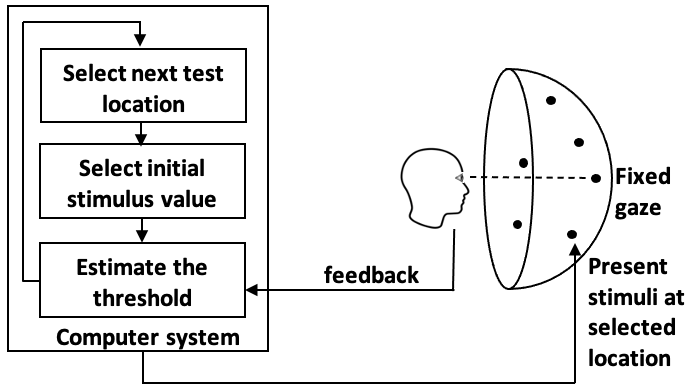
As shown in Figure 1, the perimetry test can be divided into three critical decision-making steps: (1) selection of the next testing location, (2) determination of the initial stimulus intensity to be presented at the next location, and (3) estimation of the sensitivity threshold at that location. This sequential decision-making problem is characterized by uncertainty, as the patient’s response to the presented stimuli is probabilistic. Reinforcement learning (RL) presents a suitable approach for optimizing the perimetry test, as it can determine the optimal sequence of locations and initial stimulus values to be tested to maximize speed and accuracy. In this paper, we propose RLPeri, an RL-based perimetry strategy, which focuses on optimizing the entire visual field testing procedure. For the third step, we use Zippy Estimation by Sequential Testing (ZEST) (King-Smith et al. 1994) method to estimate the sensitivity threshold at each location. Our approach differs from recent works, such as Patient-Adaptive Sampling Strategy (PASS) (Kucur et al. 2019), which only selects a predefined number of locations to be tested. Our method optimizes the entire visual field testing sequence and shows improved test accuracy compared to PASS. Our proposed method is designed to address the requirement for higher accuracy in clinics. In this particular case, selecting fewer locations like PASS is insufficient to meet this requirement.

Since the 1970s, perimetry tests has been automated by computer algorithms (Johnson, Wall, and Thompson 2011). These algorithms have a trade-off between accuracy versus speed of assessment. A detailed assessment aiming for high precision and accuracy comes at the price of long testing times, patient fatigue, and consequently (and paradoxically) less reliable patient results. On the other hand, a cursory/fast assessment of the visual field may produce too imprecise/inaccurate results.

To address this trade-off between speed and accuracy, previous research has either proposed reducing the testing duration by testing only a selected number of locations (Kucur and Sznitman 2017; Kucur et al. 2019) or predicting the sensitivity threshold values (Shon, Sung, and Shin 2022; Park, Kim, and Lee 2019). In our work, we adopt a unique approach by using potential-based reward shaping to strike a balance between speed and accuracy. The potential, or reconstruction error, is calculated as the difference between the suggested initial value and the actual ground truth sensitivity value and used to shape the reward. Furthermore, in order to capture the connection between the presented stimulus at a specific location and the corresponding feedback from the patient, along with sensitivity values from neighboring locations, we represent the test state using a pair of 3D matrices. Subsequently, we employ group-wise (Krizhevsky, Sutskever, and Hinton 2012) and point-wise (Howard et al. 2017) convolution kernels to extract the relevant features from the matrices. Group-wise kernels have been demonstrated to efficiently extract features in a variety of scenarios (Douillard et al. 2020; Verma et al. 2021). In our work, this approach enables us to examine the relationship between stimuli, patient feedback, and sensitivity values across neighboring locations effectively. To summarise, following is our main contribution

• We formulate perimetry testing as a Markov Decision Process (MDP) and propose RLPeri method to determine the optimal sequence of locations and initial testing intensities for faster and more accurate results.

• We address the trade-off between speed and accuracy by utilizing potential based reward shaping. This technique uses reconstruction error as the potential of the current state, helping to achieve a balanced outcome.

• We represent test’s state as a pair of 3D matrices, and to extract features related to presented stimulus values and threshold values of neighboring locations, we utilize two distinct convolution kernels.

• Through rigorous experimentation, we demonstrate that our RLPeri approach outperforms existing state-of-the-art methods in terms of speed while maintaining the accuracy.

(a)

(b)

(c)

Figure 2: LABEL:sub@fig:sensitivity The inverse relationship between light intensity and sensitivity to light. Individuals with a high sensitivity to light are able to detect even faint lights, while those with low sensitivity to light can only see very bright lights. LABEL:sub@fig:fos Frequency-of-seeing (FOS) curve. Sensitivity threshold is defined as the intensity at which probability of seeing is 50%. Note the inverse relationship between sensitivity and stimulus intensity. LABEL:sub@fig:vf 2D mapping of sensitivity threshold values for 54 locations of 24-2 test pattern. Darker color indicates low sensitivity.

Background

In this section we briefly discuss about perimetry, ZEST procedure and reinforcement learning.

Perimetry

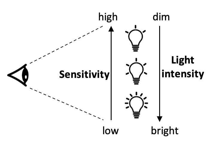
Perimetry testing is a crucial procedure in ophthalmology to assess a patient’s visual field and sensitivity thresholds. The test is done by presenting light stimuli of different intensities (in decibels, dB) at different locations of visual field. The relationship between stimulus intensity and a patient’s sensitivity to light is inverse. As shown in Figure 2a, a patient with a high sensitivity to light can see with a low-intensity stimulus, whereas a patient with low sensitivity to light requires a high-intensity stimulus. The sensitivity to light is measured in decibels (dB) as follows

$$dB=10*log(L_{max}/L)$$ (1)

Where $L_{max}$ is the maximum luminance (intensity of light reflected on the perimetric surface, measured in apostilb, asb) the perimeter can display and $L$ is luminance of the stimulus at the threshold (Racette et al. 2018). 0 dB represents the highest level of intensity that the perimetry equipment can produce.

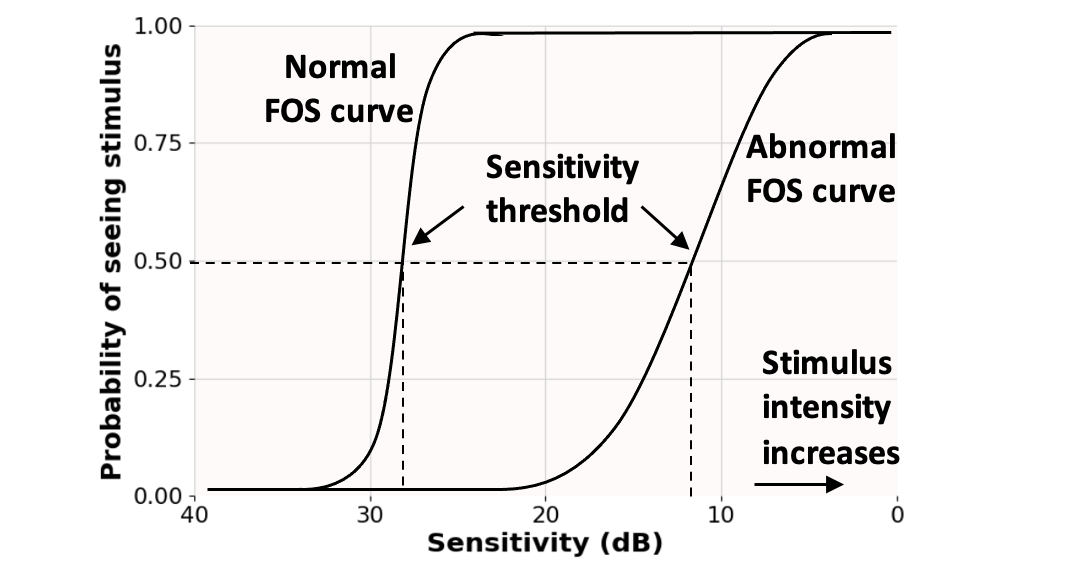
Following stimulus presentation, the patient responds seen/not seen depending on their ability to perceive the stimulus. Based on their response, the intensity of the stimuli is adjusted until the sensitivity threshold is estimated for that specific location. The procedure is then repeated again for the next location till the sensitivity threshold is estimated for all the visual field locations. However, it is a noisy process and same patient always show slightly varying responses if test is repeated. In short, the likelihood of seeing or not seeing is probabilistic, especially for stimuli values near threshold value. The sensitivity threshold is defined as the intensity of light that can be perceived by the patient 50% of the time. Figure 2b depicts frequency-of-seeing (FOS) curve, which describes the probability that a patient will see a target as a function of the intensity of the stimulus. The FOS curve on the left with a threshold value of 32 dB represents a normal eye, while the FOS curve on the right with a lower threshold value indicates some visual defect. A sensitivity threshold of 0 dB means that the patient is not able to see the most intense stimulus that the perimetry equipment can produce.

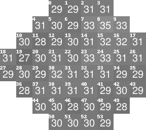
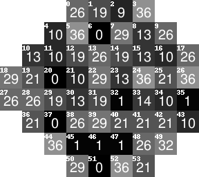
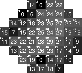
The number of locations in the visual field varies depending on the test pattern, for example a 24-2 test strategy (Henson 1993) test 54 locations. Figure 2c illustrates a 2D representation of visual fields specific to the 24-2 test strategy. The visualization includes sensitivity threshold values (measured in dB) at the center and location identifiers placed in the upper left corner. The threshold values generally varies from 0-40 dB.

ZEST Procedure

The ZEST (King-Smith et al. 1994) procedure involves associating each visual field location with a probability density function (pdf), which characterizes the probability that a specific stimulus value is the threshold for that location. Initial pdf, a likelihood function and a stopping criteria are key components of ZEST. The test at a given location begins with an initial pdf. Subsequently, the procedure iteratively refines the pdf by incorporating the patient’s responses and the likelihood function. The test at that location concludes when the stipulated stopping criterion is met. One possible way to stop the test is to terminate it when the standard deviation of the pdf is lower than a predetermined value (Turpin et al. 2002), which we used in our experiments.

Reinforcement Learning

Reinforcement Learning (Sutton and Barto 1998) is a popular method for solving Markov Decision Process (MDP) when the model of MDP is not known. An MDP is formally defined as the tuple $\big{\langle}{\mathcal{S,A,T,R}}\big{\rangle}$, where $\mathcal{S}$ is the set of states, $\mathcal{A}$ is the set of actions, $\mathcal{T}(s,a,s^{\prime})$ represents the probability of transitioning from state $s$ to state $s^{\prime}$ on taking action $a$ and $\mathcal{R}(s,a)$ represents the reward obtained on taking action $a$ in state $s$. RL agents learn a policy that maximizes their expected future reward while interacting with the environment. Q-learning (Watkins and Dayan 1992) is one of the most popular RL approach, where the action value function $Q(s,a)$ are updated based on experiences given by $(s,a,s^{\prime},r)$:

$${Q}(s,a)\leftarrow(1-\alpha){Q}(s,a)+\alpha[r+\gamma\max_{a^{\prime}}Q(s^{\prime},a^{\prime})]$$ (2)

Where $\alpha$ is the learning rate and $\gamma$ is the discount factor. Advantage function $A(s,a)$ is a measure of how much action $a$ is good or bad decision in state $s$, in short it measures the advantage of selecting action $a$

$$A(s,a)=Q(s,a)-V(s)$$ (3)

where $V(s)$ is the state value function. DQN (Mnih et al. 2015) approximates the Q-values with a deep neural network. This deep network for Q-values is parameterized by a set of parameters, $\theta$ and the parameters are learned using an iterative approach that employs gradient descent on the loss function. Specifically, the loss function at each iteration is defined as follows:

$$\mathcal{L}_{\theta}=\mathbb{E}[(y^{DQN}-Q(s,a;\theta))^{2}]$$ (4)

where $y^{DQN}=r+\gamma\text{max}_{a^{\prime}}Q(s^{\prime},a^{\prime};\theta^{-})$ is the target value computed by a target network parameterized by previous set of parameters, $\theta^{-}$. Parameters $\theta^{-}$ are frozen for some time while updating the current parameters $\theta$. To ensure independence across experiences this approach maintains a replay memory ${\mathcal{J}}$ and then samples experiences from it.

Knowledge Based Learning

Knowledge based reinforcement learning deals with incorporating domain knowledge into the learning to guide exploration. Reward shaping is one of such approach which provides additional reward signal representative of prior knowledge in additional to the reward received from the environment. Reward $r$ is augmented with additional reward signal $F(s,s^{\prime})$, which is a general form of any state based reward shaping function. Reward shaping has been shown to improve learning (Ng, Harada, and Russell 1999b). However it can result into agent learning unexpected/undesired behavior if used improperly. For example, Randløv and Alstrøm (1998) demonstrated that by providing additional reward to stay balanced while learning to ride a bicycle resulted into learning a policy which preferred staying balanced and cycling in circles than reaching the destination.

To avoid such behavior, Ng, Harada, and Russell (1999a) proposed potential based reward shaping, where additional reward is computed as the difference in some potential function $\varphi$ defined over states. The potential based reward is computed as

$$F(s,s^{\prime})=\gamma\varphi(s^{\prime})-\varphi(s)$$ (5)

Where $\gamma$ is the same discount factor used in update rule provided in Equation 2. The potential of a state represents the goodness of the state, for example, potentials of states close to goal state are generally set to be more than the states that are far from the goal state. Potential based reward shaping algorithms do not alter the optimal policy.

RLPeri: Reinforcement Learning Based Perimetry

Figure 3: The test’s status is depicted using a pair of 3D matrices, encompassing the patient’s responses. Each matrix is designated for seen responses and not seen responses, respectively. Group-wise and point-wise convolutional kernels are employed to capture features related to the threshold values of the surrounding locations as well as the patient’s responses to different stimulus values presented at a given location.

As discussed in previous section, MDP is a mathematical framework that models decision making problems. In the context of visual field testing, the MDP represents the process of performing a visual field test on a patient.

State Space and State Features

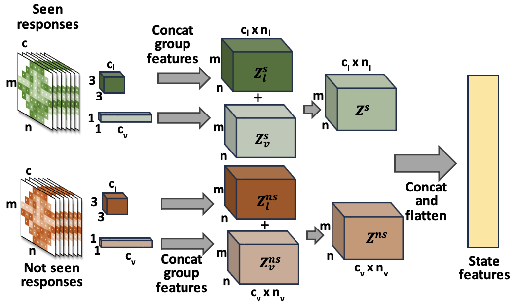
The state space of the MDP, $\mathcal{S}$, consists of all the possible visual fields that are represented as a pair of 3D matrix of size $c\times m\times n$. Here $m$ and $n$ are dependent upon the specific test pattern. For instance, in the case of the 24-2 test pattern, a total of 54 locations can be represented using an $8\times 9$ 2D matrix, with corner locations masked as demonstrated in Figure 2c. The variable $c$ denotes the number of possible stimulus values. Consequently, the state can be conceptualized as a collection of $c$ 2D matrices, each dedicated to a distinct stimulus value. First matrix compiles all the seen responses, while the second matrix accounts for all the not seen responses of the patient during testing. The entry at position $[i,j,k]$ ($i\in[1,c]$, $j\in[1,m]$, $k\in[1,n]$) of the seen matrix represents the number of times the patient was able to perceive a stimulus with an intensity of $i$ dB at location $[j,k]$. Similarly, the entry at position $[i,j,k]$ in the not seen matrix represents the number of times the patient fails to perceive the stimulus with an intensity of $i$ dB at location $[j,k]$. As discussed earlier, the patient’s ability to perceive a stimulus is probabilistic. Consequently, the algorithm may repeatedly present the same stimulus value at a chosen location. This is the reason we maintain a count of both seen and not seen responses for each stimulus value. The purpose of employing this state representation is to comprehensively capture the entirety of the patient’s responses, enabling subsequent extraction of pertinent features for the purpose of learning the state values.

Figure 3 depicts the process of extracting the state feature. We use two types of group-wise convolutional kernels, $k^{l}\in\mathbb{R}^{3\times 3\times c_{l}}$ and $K^{v}\in\mathbb{R}^{1\times 1\times c_{v}}$. $c_{l}$ and $c_{v}$ ($c_{l},c_{v}<c$) are number of channels in each group and $n_{l}$ and $n_{v}$ are number of groups in $K^{l}$ and $K^{v}$ respectively. We ensure that $c_{l}\times n_{l}=c_{v}\times n_{v}=c$. $K^{l}$ is utilized to capture spatial characteristics based on threshold values of neighboring locations, as these sensitivity thresholds often exhibit correlations. Similarly, to capture features across various stimulus values presented at a location, we employ $K^{v}$, which is a pointwise kernel. Since the patient’s ability to perceive a presented stimulus is probabilistic, if the patient is unable to perceive almost all of the consecutive stimuli in a selected stimulus intensity range, it is likely that the threshold value at that location is lower than the selected range. Conversely, if the patient successfully perceives the majority of stimuli within the selected range, it suggests that the actual threshold is likely situated above that range. This is why we use a pointwise kernel to help the model decide on the starting stimulus value. After extracting group-wise features, these features are combined to yield $Z^{s}_{l}$ and $Z^{s}_{v}$ features from the seen matrix, as well as $Z^{ns}_{l}$ and $Z^{ns}_{v}$ features from the not seen matrix. These features are then added to obtain the respective $Z^{s}$ and $Z^{ns}$ features, which are subsequently concatenated and flattened to produce the final state features.

Action Space

The set of possible visual field locations is represented by $L$, and the set of possible stimulus values is represented by $V,|V|=c$. The action taken in the MDP is represented as a tuple $(a_{l},a_{v})$, where $a_{l}\in L$ represents the location in the visual field where the stimulus is to be presented and $a_{v}\in V$ represents the stimulus value in dB. The state transition probability depends on the FOS curve for the selected location, which models the patient’s probabilistic response to the stimulus.

Reward Function

The reward function $\mathcal{R}(s,a_{l},a_{v})$ represents the negative of the number of stimuli presented to complete the test at location $a_{l}$ in the current state $s$, given that the initial stimulus value presented was $a_{v}$. To reconcile the conflicting objectives of speed (the number of stimuli presented) and accuracy (the mean squared error between the ground truth values and the constructed visual field), we use the potential based reward shaping. The potential $\varphi(s)$ of the state is represented by the negative mean squared error between the already discovered locations in the current state and their corresponding ground truth values. Consequently, during the target computation in Equation 6, $r$ is replaced with $r+F(s,s^{\prime})$, where $F(s,s^{\prime})$ is computed as outlined in Equation 5.

The action space of the MDP is huge due to its two dimensions. Hence, to tackle large action space, we use Branching Dueling Q-Network (BDQ) (Tavakoli, Pardo, and Kormushev 2018) architecture to optimize learning. Figure 4 shows the framework of RLPeri where $Q$-values of each action dimension are learned separately and independently, allowing for more effective and efficient learning. The shared state representation allows for estimation of both the state values and advantages of each action dimension, resulting in improved overall performance. We define $Q_{l}(s,a;\theta)$ and $Q_{v}(s,a;\theta)$ as the parameterised action-value functions for location dimension and stimuli value dimension actions. Here $\theta$ is the network parameter. These values are estimated using the state value function $V(s,\theta)$ and the advantage functions $A(s,a_{l},\theta)$ and $A(s,a_{v},\theta)$ as follows

Figure 4: Framework for RLPeri. Q-values are learned independently for each action dimension.

$$Q_{l}(s,a;\theta)=V(s,\theta)+\Big{(}A(s,a_{l};\theta)-\dfrac{1}{|L|}\sum_{a_{l}^{\prime}}A(s,a_{l}^{\prime};\theta)\Big{)}$$

$$Q_{v}(s,a;\theta)=V(s,\theta)+\Big{(}A(s,a_{v};\theta)-\dfrac{1}{|V|}\sum_{a_{v}^{\prime}}A(s,a_{v}^{\prime};\theta)\Big{)}$$

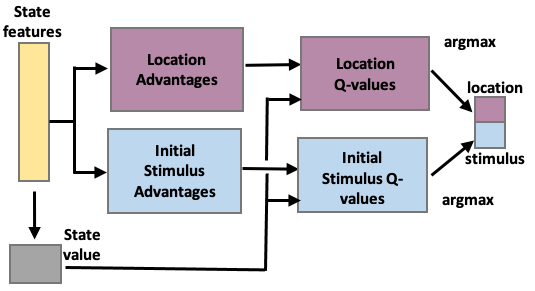
After estimating Q-values for each action dimension, the target values are computed by averaging the next state’s action-values for each dimension. For experience $<s,a_{l},a_{v},r,s^{\prime}>$, the target value is computed as follows

$$y=r+ \gamma\dfrac{1}{2}\Big{[}Q_{l}\Big{(}s^{\prime},\mathrm{argmax}_{a^{\prime}_{l}}Q_{l}(s^{\prime},a^{\prime}_{l};\theta);\theta^{-}\Big{)}$$

$$+Q_{v}\Big{(}s^{\prime},\mathrm{argmax}_{a^{\prime}_{v}}Q_{v}(s^{\prime},a^{\prime}_{v};\theta);\theta^{-}\Big{)}\Big{]}$$ (6)

Finally, the the network is trained on batch of experiences replayed from the replay memory ($\mathcal{J}$) by computing loss values for each action dimension. The loss function is defined as

$$\mathcal{L}=\mathbb{E}_{(s,a_{l},a_{v},r,s^{\prime})\sim\mathcal{J}}\Big{[}\dfrac{1}{2}\big{[}\big{(}y-Q_{l}(s,a_{l};\theta)\big{)}$$

$$+\big{(}y-Q_{v}(s,a_{v};\theta)\big{)}\big{]}\Big{]}^{2}$$ (7)

The training is episodic where one complete visual field test (i.e. all $L$ locations have been tested) is considered as one episode. RLPeri uses $\epsilon-$greedy exploration (Sutton and Barto 1998) to generate learning episodes. Experiences $<s,a_{l},a_{v},r,s^{\prime}>$ are used to update the learning. After selecting next location $a_{l}$ and corresponding starting stimulus value $a_{v}$, ZEST is used to estimate the threshold value at the location. The detailed steps of RLPeri and ZEST are provided in the Appendix.

Experiments

In this section we discuss our experimental results in detail. We first describe our dataset and simulator.

Dataset

We evaluated our approach on Rotterdam visual field data set (Erler et al. 2014). It includes 5108 visual field samples from 22 healthy and 139 glaucomatous patients. Visual Fields were acquired using 24-2 pattern (54 locations). We divided the data set into training data (60%), test data (20%) and validation data (20%).

Simulator

To train and evaluate RLPeri, we created a realistic simulator using the dataset. As mentioned, the patient responses are probabilistic, with the likelihood of a seen or not seen response being dependent on the location’s FOS curve. The ground truth data only provides visual field maps with corresponding sensitivity threshold values, but does not include the actual FOS curve. To address this, we estimated the FOS curve for each location by fitting a normal cumulative distribution function to the ground truth threshold value, with a fixed standard deviation of 1.

In RLPeri, each complete VF test is treated as a single learning episode. At the start of each episode, the initial state is represented with two 3D matrices of size $41\times 8\times 9$, one each for seen and not seen matrix. Non-VF locations (corner locations if we represent 2D map of Figure 2c using $8\times 9$ matrix) in the each 2D matrix are initialized to -2 while valid VF locations are initialized with a count of 0. During training and testing, the simulator presents a stimulus value to a location and simulates a seen or not seen response based on the estimated FOS curve and its corresponding probability distribution. In order to simulate the responses of seen and not seen at a particular location for a given stimulus, we generate a random number between 0 and 1. Let p represent the probability of seeing at that location for the presented stimulus, as determined by the FOS curve. If the randomly generated number is less than or equal to p, we assume that the stimulus was seen. Otherwise, if the generated number is greater than p, we consider the stimulus to be not seen. The sate moves to the next state based on these responses.

We employed a stimulus value range of 0 to 40 dB. After determining next location to be tested and initial stimulus value, we use ZEST to estimate the final sensitivity threshold value at the location to reconstruct the VF. As described in the background section, initial probability density function (pdf) for each location is needed. The training dataset was utilized to calculate the frequency distribution of sensitivity values at each location, which was subsequently employed to formulate the initial pdf for each location. Similarly, we assumed liklihood function to be a gaussian function with presented stimuli as mean and a fixed standard deviation of 0.5 dB. We used standard deviation (represented as $\sigma$ in experimental results) of the estimated pdf as the stopping criteria. When $\sigma$ of estimated pdf falls below a predefined value (we experimented with $\sigma=1,2,3$), the testing at the location is considered to be complete.

Evaluation Metric

We used two different metrics to compare the performances. First one is total number of stimuli presented to complete the visual field test. As time taken to complete the test is linearly correlated with total number of stimuli presented, we use total number of stimuli presented as the proxy of speed of the visual field test. Mean Squared Error (MSE) between the ground truth visual field and the reconstructed visual field is used as the second evaluation metric. As illustrated in Equation 1, the correlation between sensitivity and light intensity is non-linear. Similarly, the relationship between visual function and light intensity exhibits non-linearity. For example, a 90 asb increase is noticeable when intensity goes from 10 to 100 asb, but the same increase is hardly noticeable when it goes from 1,000 to 1,090 asb (Racette et al. 2018). This method of measuring sensitivity from light intensity effectively imparts linearity to the relationship between dB and intensity. Therefore, the visual effect difference between higher dB values (such as 24 dB and 30 dB) is similar to the visual effect difference between lower dB values (such as 2 dB and 8 dB). This characteristic makes MSE an appropriate metric for assessing accuracy.

The experiments were carried out across five separate seeds, and the results encompass both the reported mean values and their respective standard deviations. In the Appendix, we additionally conduct a qualitative analysis of the generated sequence of locations and initial stimulus values across multiple visual fields.

Hyperparameter and Computing Infrastructure

We used Adam optimizer (Kingma and Ba 2014) to perform mini-batch stochastic gradient descent optimization. We also use dropout layer and layer normalization to prevent the network from overfitting. We set number of groups in $K^{l}$ to 8 and number of groups in the pointwise convolutional kernel $K^{v}$ to 4. We used 1e-4 as learning rate after tuning it in the range of 1e-2-1e-4. The batch size was set to 2048. We performed $\epsilon$-greedy exploration and it was decayed exponentially. We stopped decaying $\epsilon$ once its value reached to 0.01. We also use validation error while training to select the best model. Our experiments were conducted on a 64-bit Ubuntu machine equipped with 500GB of memory and a 40GB GPU. For deep learning tasks, we employed the PyTorch framework.

Results

$\sigma$	Method	Number of	MSE
		stimuli presented
1	ZEST	348.15 (0.66)	0.949 (0.005)
	SORS	364.62 (0.66)	0.943 (0.007)
	RLPeri	310.56 (3.2)	0.938 (0.013)
2	ZEST	278.68 (0.54)	1.475 (0.01)
	SORS	295.93 (0.36)	1.454 (0.009)
	RLPeri	240.94 (2.48)	1.448 (0.027)
3	ZEST	258.41 (0.53)	1.897 (0.017)
	SORS	279.29 (0.32)	1.764 (0.016)
	RLPeri	221.19 (3.10)	1.906 (0.083)
-	PASS	108.07 (14.76)	15.03 (14.87)
-	TOP	54.00 (0.00)	32.35 (12.99)
-	DS	156.31 (12.81)	15.17 (11.04)

Table 1: Performance of different perimetry strategies. Mean and standard deviation is provided for number of stimuli presented and MSE. Results are aggregated over five different runs.

We use ZEST method with random sequence of locations and random initial stimulus values as our baseline method. We also compare with SORS (Kucur and Sznitman 2017), PASS (Kucur et al. 2019), DS (Weber, Dannheim, and Dannheim 1990) and TOP strategy (Morales, Weitzman, and de la Rosa 2000). SORS determines sequence of locations to be tested for reconstructing VFs more accurately and uses these reconstructed values to determine the threshold. Similar to RLPeri, it uses ZEST to estimate sensitivity threshold at a location. Unlike the SORS paper, we chose not to enforce the maximum limit of 4 stimuli per location in our implementation to ensure fairness in comparison. PASS is an RL based method that uses a predetermined number of test locations to estimate sensitivity thresholds at different locations in the visual field. On the other hand, both DS and TOP use sensitivity threshold of tested neighbour locations as the starting stimuli value. TOP tests each location only once, yielding very fast VFs with low-accuracy. For DS and TOP, we use results presented in paper (Kucur et al. 2019).

Table 1 provides experimental results for RLPeri and other methods. $\sigma$, which is the stopping criteria for ZEST, is the predefined value of the standard deviation of the pdf. As can be seen, with increasing value of $\sigma$, MSE error increases and number of stimuli needed to complete the testing decreases. This is expected as for more accurate estimate of sensitivity threshold, a location needs to be tested with high number of stimuli. For all the values of $\sigma$, RLPeri is the fastest with comparable accuracy as compared to ZEST and SORS. Though MSE values are very close (which is expected as it is dependent on ZEST’s stopping criteria), paired t-test confirmed that they are significantly different at a p-value of 1%. This indicates that starting stimulus value and the sequence of testing locations do impact the accuracy. Overall, depending on the stopping criteria, RLPeri is faster than ZEST by around 10-15% and faster than SORS by around 15-20%.

TOP is a fast method as it tests each location with only one stimuli, but its accuracy is low with a high MSE of 32.35. Likewise DS is fast with 156.31 stimuli presented, it has a high MSE of 15.17. As RLPeri tests every location, for fair comparison we include results for PASS with every location tested. Although PASS is faster (108.07 number of stimuli), its MSE is high at 15.03. RLPeri’s effectiveness is demonstrated by the low number of stimuli presented while maintaining the accuracy.

Ablation Studies

To demonstrate the efficacy of reward shaping technique, we conduct ablation studies employing different reward functions. The outcomes of these studies are summarized in Table 2. The num stimuli reward type employs the number of stimuli required to conclude the test as the reward function, the reconstruction reward type employs the MSE as the reward function, and the shaping reward type corresponds to the reward shaping approach detailed in previous section. Ideally, the num stimuli reward type would prioritize speed over accuracy. Surprisingly, our observations revealed that employing the number of stimuli as a reward did not consistently result in policies that generated faster tests. This might be attributed to the fact that it overlooked the importance of recommending optimal initial stimulus values. Conversely, the reconstruction reward type, as anticipated, led to relatively slower tests while achieving marginally enhanced accuracy. Reward shaping demonstrates consistent performance, contrasting with the other two methods, as evidenced by its reduced variance (as indicated by the standard deviation within parentheses). These results suggest that reward shaping can be leveraged to strike a balance between speed and accuracy. In the Appendix, we offer a comparative analysis by employing a 2D matrix to represent the state, in contrast to the proposed utilization of a pair of 3D matrices.

$\sigma$	Reward	Number of	MSE
	type	stimuli presented
1	num stimuli	329.42 (33.72)	0.952 (0.013)
	reconstruction	347.09 (30.43)	0.932 (0.004)
	shaping	310.56 (3.2)	0.938 (0.013)
2	num stimuli	254.32 (26.43)	1.482 (0.033)
	reconstruction	276.25 (35.50)	1.442 (0.009)
	shaping	240.94 (2.48)	1.448 (0.027)
3	num stimuli	216.82 (4.92)	1.978 (0.166)
	reconstruction	251.19 (31.77)	1.82 (0.095)
	shaping	221.19 (3.10)	1.906 (0.083)

Table 2: Ablation studies. Results are aggregated over five different runs.

Related Work

Researchers aim to accelerate visual field testing by developing methods that efficiently manipulate stimuli values at a location. SITA (Swedish Interactive Thresholding Algorithm) is a family of visual field testing methods that uses a Bayesian adaptive approach to estimate the patient’s threshold sensitivity at each location in the visual field. These algorithms also estimate the level of certainty with which the threshold is known at each point, and testing is stopped at each test location based on predetermined levels of threshold certainty. SITA standard (Bengtsson et al. 1997) is the original algorithm whereas SITA Fast (Bengtsson and Heijl 1998) and SITA Faster (Heijl et al. 2019) were developed as faster alternatives to SITA standard, with SITA Faster being the fastest but also the least accurate. To estimate threshold value at a location, ZEST (King-Smith et al. 1994) assigns a prior probability density function (pdf) to the visual field location, which represents the likelihood of a particular stimuli value being the sensitivity threshold of that location. In our work we use ZEST to determine the sensitivity threshold at a specific location.

Some methods find initial stimulus values by considering the interdependence of thresholds at neighboring locations, aiming to choose stimuli values that maximize information gained per stimulus. For example, DS (Dynamic Strategy) (Weber, Dannheim, and Dannheim 1990) method uses the sensitivity threshold of the neighboring locations as the starting stimuli value, and adjusts the stimuli values at each location based on the response obtained at the previous location. Likewise, GOANNA (Gradient-Oriented Automated Natural Neighbor Approach) (Chong et al. 2014) uses a technique called natural neighbor interpolation to estimate the visual field sensitivity at untested locations based on the sensitivity values at tested locations. SWeLZ (Spatially Weighted Likelihoods in Zest) (Rubinstein, McKendrick, and Turpin 2016) is a modification of the ZEST algorithm that takes into account the spatial relationships between adjacent locations in the visual field.

Efforts have been made to decrease the number of locations required to complete the visual field test in order to further expedite the process. In TOP (Tendency Oriented Perimetry) (Morales, Weitzman, and de la Rosa 2000), the stimuli are presented only once at each location, and the test sequence is predetermined based on the location’s tendency to have a visual field defect. SEP (Spatial entropy pursuit) (Wild, Kucur, and Sznitman 2017) utilizes entropy, which quantifies the level of uncertainty or randomness in a system, to identify the most informative locations to test and thereby minimize the number of required test locations.

Another research direction is to find optimal sequence of these locations. SORS (Sequentially Optimized Reconstruction Strategy) (Kucur and Sznitman 2017) uses an adaptive algorithm to determine the order in which visual field locations are tested to reconstruct the visual field with the greatest accuracy. Conversely, PASS (Patient-Adaptive Scheduling System) (Kucur et al. 2019) employs reinforcement learning to determine the optimal sequence of a predetermined number of test locations to estimate sensitivity thresholds. However, these methods often prioritize either speed (PASS) or accuracy (SORS). Our approach aligns with this category, utilizing reinforcement learning to determine the optimal sequence for locations during visual field testing and implementing reward shaping to strike a balance between speed and accuracy. Our experimental results demonstrate that our proposed method is faster than SORS and more accurate than PASS.

Conclusion

In this study, we introduce RLPeri, a reinforcement learning-based strategy to optimize visual perimetry testing. Our approach focuses on determining an optimal sequence of locations and initial stimulus values, aiming to reduce examination time while maintaining accuracy. Incorporating reward shaping techniques further enhances testing performance. By representing the test’s state with 3D matrices and employing specialized convolutional kernels, we extract spatial and stimulus-specific features. Our experiments reveal a noteworthy 10-20% decrease in examination time while preserving accuracy. This finding points towards a promising avenue for improving the efficiency and user-friendliness of visual perimetry testing, a critical procedure in diagnosing and monitoring conditions like glaucoma and other ocular and neurological disorders.

Appendix: RLPeri: Accelerating Visual Perimetry Test with Reinforcement Learning and Convolutional Feature Extraction

Appendix A RLPeri

In this section, we present a comprehensive overview of the RLPeri approach and the underlying ZEST algorithm. Algorithm 1 outlines the detailed steps involved in learning action-values using RLPeri, which employs $\epsilon$-greedy exploration to generate learning episodes. Testing all $L$ locations based on a ground truth visual field is considered as an episode where ground truth values are used to generate seen and not seen responses and computing reconstruction errors. Upon selecting the next location $a_{l}$ and the corresponding initial stimulus value $a_{v}$, ZEST is employed to determine the reward $r$, representing the negative of the number of steps taken to complete the test at location $a_{l}$, and the estimated sensitivity threshold $v$ at that location. Reward shaping is applied based on potential values of current state and next state. Subsequently, after collecting experiences $<s,a_{l},a_{v},r,s^{\prime}>$, the algorithm iteratively updates network parameters to minimize loss, facilitating convergence.

Algorithm 1 RLPeri

Input: Ground truth visual fields $G$, stopping standard deviation value $\sigma$.
Output: Trained model.

1:  Initialize replay buffer $\mathcal{J}$, action-value functions $Q_{l}(s,a;\theta)$, $Q_{v}(s,a;\theta)$ and target functions $Q_{l}(s,a;\theta^{-})$, $Q_{v}(s,a;\theta^{-})$

2:  Initialize initial probability density function, $init\_pdf$ for every location

3:  while not converged do

4:     for $g\in G$ do {Loop over ground truth VFs}

5:        Initialize seen and not seen matrices to get current state $s$

6:        Initialize threshold values $pred[i]=-1,i\in L$

7:        Initialize frequency of seeing $fos$ for every location based on $g$

8:        for $i\in|L|$ do {Loop over number of testing locations}

9:           Compute potential $\varphi(s)$ based on $g$ and $pred$

10:           With probability $\epsilon$, select random action$\quad a_{l}\leftarrow\text{random location from untested locations}$ $\quad a_{v}\leftarrow\text{random initial stimulus value}$ With remaining probability $1-\epsilon$ $\quad a_{l}\leftarrow\underset{a^{\prime}_{l}}{\mathrm{argmax}}Q_{l}(s,a^{\prime}_{l};\theta)$ $\quad a_{v}\leftarrow\underset{a^{\prime}_{v}}{\mathrm{argmax}}Q_{v}(s,a^{\prime}_{v};\theta)$

11:           Estimate threshold using ZEST, receive corresponding reward and move to next state$\quad-r,v,s^{\prime}\leftarrow ZEST(a_{v},init\_pdf[a_{l}],fos[a_{l}],s,\sigma)$

12:           $pred[a_{l}]=v$

13:           Compute potential $\varphi(s^{\prime})$ based on $g$ and $pred$

14:           $r\leftarrow r+\gamma\varphi(s^{\prime})-\varphi(s)$

15:           $s\leftarrow s^{\prime}$

16:           Store experience $<s,a_{l},a_{v},r,s^{\prime}>$ in the replay memory $\mathcal{J}$

17:        end for

18:        Periodically update the network parameters $\theta$ by sampling experiences from $\mathcal{J}$ and minimizing the loss function $\mathcal{L}=\mathbb{E}_{(s,a_{l},a_{v},r,s^{\prime})\sim\mathcal{J}}\Big{[}\dfrac{1}{2}\big{[}\big{(}y-Q_{l}(s,a_{l};\theta)\big{)}+\big{(}y-Q_{v}(s,a_{v};\theta)\big{)}\big{]}\Big{]}^{2}$

19:        Periodically update the target network parameters

20:     end for

21:  end while

22:  return $Q_{l}(s,a;\theta)$, $Q_{v}(s,a;\theta)$

The details of ZEST is provided in Algorith 2. It estimates threshold values during perimetry testing. It begins with an initial stimulus value and iteratively adjusts the probability density function based on patient responses and likelihood. The algorithm stops when stopping criterion is met. It returns the number of stimuli presented, estimated threshold value, and the next state.

Algorithm 2 ZEST

Input: Initial stimulus value $a_{v}$, initial pdf $init\_pdf$, probability of seeing $p$, current state $s$, stopping criteria $\sigma$.
Output: Number of stimuli presented $n$, estimated threshold value $v$, next state $s^{\prime}$.

1:  $n=0,v=a_{v},min=0,max=40$

2:  $vals=[min,...,max]$

3:  $terminate=False$

4:  while $!terminate$ and $v\geq min$ and $v\leq max$ do

5:     $rand=U(0,1)$ {sample from uniform distribution}

6:     Determine patient’s response, $resp=(p>rand)$

7:     Update state to $s^{\prime}$ based on response

8:     Get likelihood function, $l=likelihood(resp,v,vals)$

9:     Update the pdf estimate, $pdf=pdf*l$

10:     $pdf=norm(pdf)$

11:     $terminate=std(pdf)<\sigma$

12:     $v=argmax(pdf)$

13:  end while

14:  return $n,v,s^{\prime}$

1:  Function $likelihood$ ($resp,v,vals$):

2:  $l=Gaussian\_cdf(vals,mean=v,std=1)$

3:  $l=resp*(resp-l)+(1-resp)*l$

4:  return $l$

Appendix B Ablation Studies

In this section, we present a comparison of results obtained when utilizing a 2D matrix to represent the state, as opposed to the proposed approach using a pair of seen and not seen matrices. Additionally, we offer a qualitative analysis of the generated sequence of locations and initial stimulus values across multiple visual fields.

State Representation

To assess the effectiveness of the proposed state representation using a pair of 3D matrices, we conduct a comparison with an alternative state representation. The alternative approach involves representing the state as a 2D matrix, where visual locations are mapped onto the matrix and estimated threshold values are assigned as the entries. We used a $8\times 9$ matrix to represent the 54 locations, masking the corner locations that do not belong to the visual field. Specifically, the non-visual field locations were assigned a constant value of -2. For the remaining locations, we initialized the threshold sensitivity values to values outside the valid range (-1), which were subsequently updated withe estimated threshold values during testing.

Table 3 shows the results for different $\sigma$ values. During training, reward shaping was employed for both type of state representation. The number of stimuli presented (indicative of speed) and MSE (accuracy) values both exhibit inferior performance with the 2D state representation. Moreover, the high variance indicates inconsistent performance when using the 2D matrix state representation. This observation supports our assertion that representing the state as a pair of seen and not seen matrices leads to more efficient extraction of state features, resulting in the learning of improved policies.

Table 3: Ablation studies. Mean and standard deviation is provided for number of stimuli presented and MSE. Results are aggregated over five different runs.

$\sigma$	State	Number of	MSE
	type	stimuli presented
1	2D state	328.99 (14.26)	0.952 (0.008)
	3D state	310.56 (3.2)	0.938 (0.013)
2	2D state	257.41 (10.9)	1.486 (0.009)
	3D state	240.94 (2.48)	1.448 (0.027)
3	2D state	235.67 (21.42)	1.965 (0.091)
	3D state	221.19 (3.10)	1.906 (0.083)

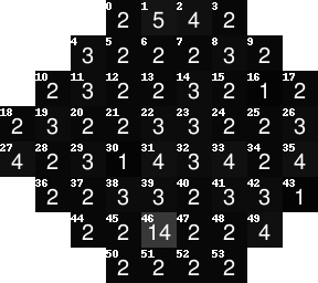
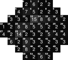
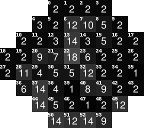
Qualitative Analysis

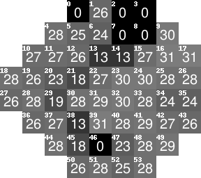
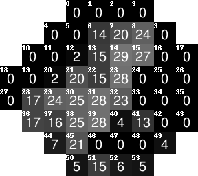
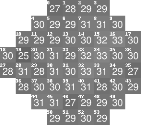
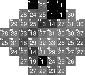
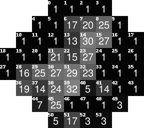
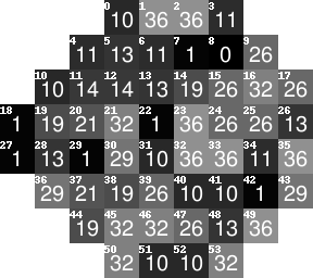
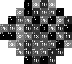
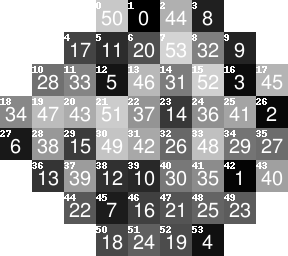
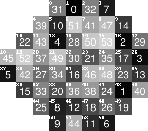
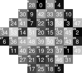
Figure 5 provides a qualitative understanding of RLPeri by displaying ground truth values, reconstructed VFs, initial stimulus values, the sequence of testing locations, and the number of stimuli presented at each location for different visual fields. We selected three visual fields with varying degree of sensitivities and we used stopping criterion $\sigma=3$. The ground truth VFs are represented in Figures 5a-5c with darker shades indicating lower sensitivity. The corresponding reconstructed VFs are displayed in Figures 5d-5f. The sequence of testing locations used is depicted in Figures 5j-5l, with darker shades indicating early tested locations. Figures 5m-5o illustrate the number of stimuli presented (following the ZEST algorithm) at each location. The total number of stimuli presented were 146 for VF A, 219 for VF B, and 300 for VF C. The reconstruction MSE errors were 1.56, 1.80 and 2.07 respectively. It is interesting to note that due to probabilistic responses, presenting initial stimulus values closer to the ground truth value does not necessarily result in fewer stimuli presented to estimate the threshold. For instance, for VF A, even if the initial stimulus value of 32 (Figure 5g) for location 46 is close to the ground truth value of 28 (Figure 5a), it still required 14 stimuli (Figure 5m) to estimate the threshold. On the contrary, even if the initial stimulus value of 26 (Figure 5i) at location 0 (Figure 5l) is far from the ground truth value of 0 (Figure 5c), it only took 2 stimuli (Figure 5o) to estimate the threshold as 1 (Figure 5f). Figures 5j-5l demonstrate that the sequence of initial tested locations (darker shade locations) are similar when a test is started, however the sequence changes as the test proceeds and threshold values are estimated. This observation indicates that the algorithm has learned to suggest the next location based on the current state. Similarly, the recommendation for initial stimulus value also improves as testing progresses.

(a) Ground truth A

(b) Ground truth B

(c) Ground truth C

(d) Reconstructed VF A

(e) Reconstructed VF B

(f) Reconstructed VF C

(g) Initial stimulus value A

(h) Initial stimulus value B

(i) Initial stimulus value C

(j) Sequence of locations A

(k) Sequence of locations B

(l) Sequence of locations C

(m) Number of stimuli A

(n) Number of stimuli B

(o) Number of stimuli C

Figure 5: Ground truth values, reconstructed visual fields, initial stimulus presented, sequence of locations and number of stimuli presented at each location for testing of three different visual fields A, B and C.

References

- Bengtsson and Heijl (1998) Bengtsson, B.; and Heijl, A. 1998. SITA Fast, a new rapid perimetric threshold test. Description of methods and evaluation in patients with manifest and suspect glaucoma. Acta Ophthalmologica Scandinavica, 76(4): 431–437.
- Bengtsson, Heijl, and Olsson (1998) Bengtsson, B.; Heijl, A.; and Olsson, J. 1998. Evaluation of a new threshold visual field strategy, SITA, in normal subjects. Swedish Interactive Thresholding Algorithm. Acta Ophthalmologica Scandinavica, 76(2): 165–169.
- Bengtsson et al. (1997) Bengtsson, B.; Olsson, J.; Heijl, A.; and Rootzén, H. 1997. A new generation of algorithms for computerized threshold perimetry, SITA. Acta Ophthalmologica Scandinavica, 75(4): 368–375.
- Chauhan and Johnson (1999) Chauhan, B.; and Johnson, C. 1999. Test-retest variability of frequency-doubling perimetry and conventional perimetry in glaucoma patients and normal subjects. Investigative ophthalmology & visual science, 40(3): 648–656.
- Chong et al. (2014) Chong, L. X.; McKendrick, A. M.; Ganeshrao, S. B.; and Turpin, A. 2014. Customized, automated stimulus location choice for assessment of visual field defects. Investigative ophthalmology & visual science, 55(5): 3265–3274.
- Douillard et al. (2020) Douillard, A.; Cord, M.; Ollion, C.; Robert, T.; and Valle, E. 2020. Podnet: Pooled outputs distillation for small-tasks incremental learning. In Computer Vision–ECCV 2020: 16th European Conference, Glasgow, UK, August 23–28, 2020, Proceedings, Part XX 16, 86–102. Springer.
- Erler et al. (2014) Erler, N. S.; Bryan, S. R.; Eilers, P. H.; Lesaffre, E. M.; Lemij, H. G.; and Vermeer, K. A. 2014. Optimizing structure–function relationship by maximizing correspondence between glaucomatous visual fields and mathematical retinal nerve fiber models. Investigative ophthalmology & visual science, 55(4): 2350–2357.
- Heijl et al. (2019) Heijl, A.; Patella, V. M.; Chong, L. X.; Iwase, A.; Leung, C. K.; Tuulonen, A.; Lee, G. C.; Callan, T.; and Bengtsson, B. 2019. A new SITA perimetric threshold testing algorithm: construction and a multicenter clinical study. American Journal of Ophthalmology, 198: 154–165.
- Henson (1993) Henson. 1993. Visual Fields. In Visual Fields. Oxford: Oxford University Press.
- Howard et al. (2017) Howard, A. G.; Zhu, M.; Chen, B.; Kalenichenko, D.; Wang, W.; Weyand, T.; Andreetto, M.; and Adam, H. 2017. Mobilenets: Efficient convolutional neural networks for mobile vision applications. arXiv preprint arXiv:1704.04861.
- Johnson, Wall, and Thompson (2011) Johnson, C. A.; Wall, M.; and Thompson, H. S. 2011. A history of perimetry and visual field testing. Optometry and Vision Science, 88(1): E8–E15.
- King-Smith et al. (1994) King-Smith, P. E.; Grigsby, S. S.; Vingrys, A. J.; Benes, S. C.; and Supowit, A. 1994. Efficient and unbiased modifications of the QUEST threshold method: theory, simulations, experimental evaluation and practical implementation. Vision research, 34(7): 885–912.
- Kingma and Ba (2014) Kingma, D. P.; and Ba, J. 2014. Adam: A method for stochastic optimization. arXiv preprint arXiv:1412.6980.
- Krizhevsky, Sutskever, and Hinton (2012) Krizhevsky, A.; Sutskever, I.; and Hinton, G. E. 2012. Imagenet classification with deep convolutional neural networks. Advances in neural information processing systems, 25.
- Kucur et al. (2019) Kucur, Ş. S.; Márquez-Neila, P.; Abegg, M.; and Sznitman, R. 2019. Patient-attentive sequential strategy for perimetry-based visual field acquisition. Medical image analysis, 54: 179–192.
- Kucur and Sznitman (2017) Kucur, Ş. S.; and Sznitman, R. 2017. Sequentially optimized reconstruction strategy: A meta-strategy for perimetry testing. Plos one, 12(10): e0185049.
- Mnih et al. (2015) Mnih, V.; Kavukcuoglu, K.; Silver, D.; Rusu, A. A.; Veness, J.; Bellemare, M. G.; Graves, A.; Riedmiller, M.; Fidjeland, A. K.; Ostrovski, G.; et al. 2015. Human-level control through deep reinforcement learning. nature, 518(7540): 529–533.
- Morales, Weitzman, and de la Rosa (2000) Morales, J.; Weitzman, M. L.; and de la Rosa, M. G. 2000. Comparison between Tendency-Oriented Perimetry (TOP) and octopus threshold perimetry. Ophthalmology, 107(1): 134–142.
- Ng, Harada, and Russell (1999a) Ng, A. Y.; Harada, D.; and Russell, S. 1999a. Policy invariance under reward transformations: Theory and application to reward shaping. In Icml, volume 99, 278–287.
- Ng, Harada, and Russell (1999b) Ng, A. Y.; Harada, D.; and Russell, S. 1999b. Theory and application to reward shaping. In Proceedings of the Sixteenth International Conference on Machine Learning.
- Park, Kim, and Lee (2019) Park, K.; Kim, J.; and Lee, J. 2019. Visual field prediction using recurrent neural network. Scientific reports, 9(1): 1–12.
- Phu and Kalloniatis (2021) Phu, J.; and Kalloniatis, M. 2021. Viability of performing multiple 24-2 visual field examinations at the same clinical visit: the Frontloading Fields Study (FFS). American Journal of Ophthalmology, 230: 48–59.
- Racette et al. (2018) Racette, L.; Fischer, M.; Bebie, H.; Holló, G.; Johnson, C. A.; and Matsumoto, C. 2018. Visual field digest. In A guide to perimetry and the Ocotpus perimeter, volume 7, chapter 2. Haag-Streit AG.
- Randløv and Alstrøm (1998) Randløv, J.; and Alstrøm, P. 1998. Learning to Drive a Bicycle Using Reinforcement Learning and Shaping. In ICML, volume 98, 463–471. Citeseer.
- Rubinstein, McKendrick, and Turpin (2016) Rubinstein, N. J.; McKendrick, A. M.; and Turpin, A. 2016. Incorporating spatial models in visual field test procedures. Translational vision science & technology, 5(2): 7–7.
- Shon, Sung, and Shin (2022) Shon, K.; Sung, K. R.; and Shin, J. W. 2022. Can Artificial Intelligence Predict Glaucomatous Visual Field Progression? A Spatial–Ordinal Convolutional Neural Network Model. American Journal of Ophthalmology, 233: 124–134.
- Sutton and Barto (1998) Sutton, R. S.; and Barto, A. G. 1998. Reinforcement learning: an introduction MIT Press. Cambridge, MA, 22447.
- Tavakoli, Pardo, and Kormushev (2018) Tavakoli, A.; Pardo, F.; and Kormushev, P. 2018. Action branching architectures for deep reinforcement learning. In Proceedings of the AAAI Conference on Artificial Intelligence, volume 32.
- Tham et al. (2014) Tham, Y.-C.; Li, X.; Wong, T. Y.; Quigley, H. A.; Aung, T.; and Cheng, C.-Y. 2014. Global prevalence of glaucoma and projections of glaucoma burden through 2040: a systematic review and meta-analysis. Ophthalmology, 121(11): 2081–2090.
- Turpin et al. (2002) Turpin, A.; McKendrick, A. M.; Johnson, C. A.; and Vingrys, A. J. 2002. Development of efficient threshold strategies for frequency doubling technology perimetry using computer simulation. Investigative ophthalmology & visual science, 43(2): 322–331.
- Verma et al. (2021) Verma, V. K.; Liang, K. J.; Mehta, N.; Rai, P.; and Carin, L. 2021. Efficient feature transformations for discriminative and generative continual learning. In Proceedings of the IEEE/CVF conference on computer vision and pattern recognition, 13865–13875.
- Watkins and Dayan (1992) Watkins, C. J.; and Dayan, P. 1992. Q-learning. Machine learning, 8(3): 279–292.
- Weber, Dannheim, and Dannheim (1990) Weber, J.; Dannheim, F.; and Dannheim, D. 1990. The topographical relationship between optic disc and visual field in glaucoma. Acta Ophthalmologica, 68(5): 568–574.
- Wild, Kucur, and Sznitman (2017) Wild, D.; Kucur, Ş. S.; and Sznitman, R. 2017. Spatial entropy pursuit for fast and accurate perimetry testing. Investigative ophthalmology & visual science, 58(9): 3414–3424.