Machine Unlearning by Suppressing Sample Contribution

Abstract

Machine Unlearning (MU) is to forget data from a well-trained model, which is practically important due to the “right to be forgotten”. In this paper, we start from the fundamental distinction between training data and unseen data on their contribution to the model: the training data contributes to the final model while the unseen data does not. We theoretically discover that the input sensitivity can approximately measure the contribution and practically design an algorithm, called MU-Mis (machine unlearning via minimizing input sensitivity), to suppress the contribution of the forgetting data. Experimental results demonstrate that MU-Mis outperforms state-of-the-art MU methods significantly. Additionally, MU-Mis aligns more closely with the application of MU as it does not require the use of remaining data.

1 Introduction

Deep learning has achieved amazing performance by successfully learning from immense amounts of data. It is revealed that memorization of training data is a recipe for good generalization under such an overparameterization regime (Feldman, 2020; Zhang et al., 2021). Deep neural networks (DNNs) not only extract universal patterns, but also memorize specific samples (Feldman & Zhang, 2020). However, these stored public and private information can be reproduced by privacy attacks (Shokri et al., 2017; Zhu et al., 2019), raising data privacy concerns. Considering this, the sensitive data, e.g., the consuming behavior of a customer himself/herself, should has the “right to be forgotten” (RTBF, (Regulation, 2018)). This means that the data should be removed not only from the dataset but also from the trained DNN, ensuring that the DNN performs as if the data were never present in the training set. Ideally, one can retrain the model without the data that should be removed. However, it is practically impossible because training DNNs is very expensive in both time and energy. Consequently, a new and important task, called “Machine Unlearning” (MU) (Cao & Yang, 2015), has emerged. The goal of MU is to efficiently and effectively scrub information about the forgetting data from models while maintaining performance on the remaining data.

Learning is a dynamic process that gradually remembers and assimilates data (Achille et al., 2019), while unlearning is the inverse process that gradually removes data information. Thus, a line of work store historical information (e.g. parameter, gradient) during training and then subtract the related gradient updates to retrieve learning (Wu et al., 2020; Graves et al., 2021; Neel et al., 2021). Another line of work estimate training points’ impact on model parameters with influence function (Guo et al., 2020; Suriyakumar & Wilson, 2022; Mehta et al., 2022) instead of explicitly recording it. Although these methods are going ahead to the essence, it is important to note that the inverse dynamic is at least as complicated as the training process itself.

Most of the practical MU methods now follow behaviorism (Golatkar et al., 2020a, b; Chundawat et al., 2023; Tarun et al., 2023), i.e., one first models the behavior (e.g., weight distribution, activation, output, and loss) of the retrained model on the forgetting data, and then fine-tune the DNN to mimic this behavior. Theoretical modeling on weight distribution (Golatkar et al., 2020a) and activation (Golatkar et al., 2020b) rely on simplifying learning dynamics, and are quite computationally expensive. Empirical modeling mainly depends on their understanding of the distinction between training and unseen data, and then transferring knowledge for output (Chundawat et al., 2023) or learning error-maximization noise (Tarun et al., 2023) to misclassify the forgetting data. While these guidelines work well in cases where the difference is significant, they may not sufficiently ensure performance when the difference is less pronounced. Moreover, most of these guidelines impair retained performance, requiring additional maintenance by replaying the remaining data.

In this paper, we distinguish the contribution to the learned model whether a sample is involved in the training process or not. Abstractly, once the learning algorithm $\cal A$ is determined, encompassing the structure, scheme, and parameters, the resulting learned model $f$ becomes a function of the training data. In other words, the learning process is a mapping from the training set $\mathcal{D}$ to a function $f$: denoted as $f={\cal A}(\mathcal{D})$. Therefore, the training sample contributes the output: $\partial{\cal A(D)}/\partial\mathcal{D}\neq 0$ while a sample out of the training set does not. A simple but enlightening example lies in the support vector machine (Cortes & Vapnik, 1995; Christmann & Steinwart, 2008), where only the training data can act as support vectors that impact the decision boundary.

The difference in contribution to the output is conceptually significant. However, when designing a MU algorithm, we encounter two significant challenges that must be addressed. Firstly, $\cal A$ is determined by a dynamic training process, and measuring the sample contribution using the terminal state, i.e., the learned model, is difficult. To overcome this, we theoretically show that the contribution of a specific sample $x$, $\partial{\cal A(D)}/\partial x$, could be approximated by its input sensitivity $\partial{f(x)}/\partial x$ with $f=\cal A(D)$. In light of this, we propose to do Machine Unlearning via Minimizing Input Sensitivity (MU-Mis). Secondly, in DNNs, ${\cal A}$ is complicated, and data in/out of the training set could be similar either in image space or in feature space, which makes the naive sensitivity value not a very significant indicator. To address this, we investigate the input sensitivity with respect to each class. In the training process, the model gradually focuses on the target class, leading to an empirical enlargement of the discrepancy in input sensitivity between the correct class and irrelevant classes. Thus, in MU-Mis, we utilize such difference in input sensitivity as the measure of discrepancy.

We evaluate the performance of MU-Mis on standard unlearning tasks, including forgetting a full class, a sub-class, and a random subset. MU-Mis consistently outperforms state-of-the-art methods in evaluation metrics. Moreover, unlike many other methods, MU-Mis does not require the remaining data neither additional maintenance, which makes MU-Mis a more practical approach and aligns more closely with the application of MU.

Our contributions can be summarized below.

• We point out that the difference between seen and unseen data lies in their contribution to the learned model, and theoretically indicate that such contribution manifests in model sensitivity to them.

• We investigate how a sample’s contribution affects the model’s sensitivity to its own empirically. We reveal that the sample’s contribution is indicated as enlarging its own sensitivity gap between the output of its target class and irrelevant classes.

• In light of the above investigation, we convert withdrawing a sample’s contribution into withdrawing its impact on input sensitivity. Then, we propose MU-Mis, a novel unlearning method, to roll back the sensitivity gap for the forgetting data so as to eliminate the network’s response as they have never been seen.

• MU-Mis can unlearn effectively and efficiently, as evaluated on 3 unlearning tasks with comparison to 4 existing methods. Without the remaining data, MU-Mis still achieves consistent and significant improvement.

2 Related Work

Current unlearning methods can be classified into two categories (Xu et al., 2023): exact unlearning and approximate unlearning. Exact unlearning guarantees remained information of the forgetting data after unlearning statistically, while approximate unlearning aims at efficiently and effectively withdrawing data influence so that the unlearned model is undistinguishable from the retrained model. In this paper, we mainly focus on approximate unlearning, which is more practical in scenarios with limited time and resources.

Unlearning by Gradient-Based Update. Unlearning can be regarded as the inverse process of learning, by removing information of the forgetting data gradually. A line of unlearning methods keep and utilize the historical information (e.g., parameters and gradients) during training. Graves et al. (2021) withdraw gradient update of related batches, and Wu et al. (2020) perform fast retraining from intermediate checkpoints with quasi-newton method. However, due to interference of gradients between the remaining data and the forgetting data, such revocation usually damages model performance on the remaining data. Therefore, Hoang et al. (2024) project gradient update to the orthogonal subspace of the remaining data to reduce interference. Nevertheless, since learning is a progressive process, naive withdrawal of past updates can inevitably impact the model’s performance on the remaining data. Additionally, the requirement of storing historical information raises memory concerns.

Unlearning by Withdrawing Contribution to Parameters. Another line of work to address unlearning involves withdrawing the impact of the forgetting data on model parameters rather than explicitly recording it. One commonly used method for estimation is the influence function (Koh & Liang, 2017), which was first introduced to unlearning by Guo et al. (2020). However, the computation of the inverse Hessian in influence function is computationally expensive, especially for large-scale models. Therefore, follow-up work are devoted to reducing its computing overhead. Suriyakumar & Wilson (2022) avoid recalculation of Hessian inverse at every removal request with infinitesimal jackknife. Mehta et al. (2022) select a subset of important parameters to reduce matrix size. To preserve performance on the remaining data, Wu et al. (2022) patch up the damage caused by influence update through reweighting the remaining data in optimization objective. Improving from the calculation method, Peste et al. (2021) use rank-one updates to approximate the inverse of the Fisher Information Matrix (FIM). Influence-based unlearning shows potential but still hurts performance on the remaining data. This may be due to inherently inaccurate calculations. Moreover, the influence function is revealed to be fragile in DNNs (Basu et al., 2020) due to its reliance on the assumptions of convexity and optimality. Hence, there is a need for appropriate and efficient influence estimation methods tailored for DNNs.

Unlearning by Re-optimization. The above influence-based unlearning methods suffer from practical limitations, including high memory overhead and expensive computation. An alternative approach is re-optimization, where DNNs are fine-tuned to approach the retrained model by optimizing a proposed loss. This loss function is typically designed to capture the behavior of the retrained model, e.g. weight distribution, activation, output, and loss. Some work model the retrained model theoretically by depicting the learning dynamics. FisherForget (Golatkar et al., 2020a) depicts the training process with gradient flow and then minimizes the KL divergence between the weight distribution of the scrubbed network and the retrained model. However, output may still leak information due to the huge null space of parameters, they proposes minimizing the gap on activations in their follow-up work (Golatkar et al., 2020b). Theoretical modeling relies on simplifying learning dynamics, such as linearization or convexity. More efficient methods are mainly designed based on empirical insights. Empirical design relies on the distinction between seen and unseen data in model outputs or loss. Chundawat et al. (2023) propose a knowledge-transfer approach to leverage information from both useful and useless teachers for the remaining and the forgetting data. Tarun et al. (2023) propose a fast unlearning method by learning an error-maximizing noise.

3 Method

3.1 Problem Formulation

We first formulate the machine unlearning task. Denote the training dataset as $\mathcal{D}=\{x_{i},y_{i}\}_{i=1}^{N}$ and the learning algorithm $\mathcal{A}$. In Section 1, we abstractly discussed the learning model and the output of $\mathcal{A}$ is a function. For algorithm design, we parameterize the function as $f(w,x)$, where $w\in\mathbb{R}^{d}$ with $d$ being the number of parameters of the model. For a $C$-class classification problem, the output of $f$ is in $C$-dimensional space, indicating the logits to each category. Then the training is on parameters $w$ and ${\cal A}$ is a mapping from data to final parameters, i.e., ${\cal A}:\mathcal{D}\rightarrow\mathbb{R}^{d}$.

Now, we can present the well-trained model as $w_{p}=\cal{A}(\mathcal{D})$, which is called the pretrained model and serves as the start of machine unlearning. Our objective is to forget a subset of data $\mathcal{D}_{f}\subset\mathcal{D}$, in which the data are called the forgetting data. The elements in the retained subset $\mathcal{D}_{r}=\mathcal{D}\backslash{\mathcal{D}}_{f}$ is called the remaining data, and our goal of machine unlearning is to approach the retrained model, $w_{r}={\cal{A}}(\mathcal{D}_{r})$. A good unlearning mechanism should efficiently and effectively transform $w_{p}$ into a sanitized model $w_{u}$, such that the difference between $w_{u}$ and $w_{r}$ remains minimal.

3.2 Learning, Unlearning, and Input Sensitivity

Machine unlearning is to withdraw a sample’s contribution to the learning process. As discussed before, the derivative of the mapping to training data, $\partial{\mathcal{A}}/\partial{\mathcal{D}}$ conceptually reflects the contribution. However, there is no explicit expression for this mapping, and the intermediate models are usually not accessible. Therefore, it is necessary to find a surrogate for $\partial{\mathcal{A}}/\partial{\mathcal{D}}$ using only the pretrained model $w_{p}$.

Suppose the randomly initialized model is $w_{0}\in\mathbb{R}^{d}$ that corresponds to function $f_{0}\in\mathbb{R}^{C}$. Then, the iterative learning process can be written as $w_{p}=w_{0}+\sum_{k=1}^{T}\nolimits\Delta w_{k}$ with $\Delta w_{k}=w_{k+1}-w_{k}$. Specifically, when gradient descent is used, we have

$$\Delta w_{k}(\mathcal{X})=-\eta\dfrac{\partial f(w,\mathcal{X})}{\partial w}^{\top}\dfrac{\partial\mathcal{L}(\mathcal{X})}{\partial f}\bigg{|}_{w=w_{k}}.$$

In the view of function, correspondingly we have $f=f_{0}+\sum_{k=1}^{T}\Delta f_{k}$, where $\Delta f_{k}=f(w_{k+1})-f(w_{k})$.

Let us consider the mapping from model input $x$ to induced backpropogation gradient with parameters $w_{k}$, which is denoted as $g_{k}$:

$$g_{k}(\cdot)=\dfrac{\partial f(w,\cdot)}{\partial w}\bigg{|}_{w_{k}}\in\mathbb{R}^{C\times d}.$$

With the first-order expanding $f$ on $w_{k}$, we can calculate the change in function $f$ as:

$$\Delta f_{k}(x)=g_{k}(x){\Delta w_{k}(\mathcal{X})}=-\eta g_{k}(x)g_{k}(\mathcal{X})^{\top}\dfrac{\partial\mathcal{L}(\mathcal{X})}{\partial f},$$

where $g_{k}(\mathcal{X})=\sum_{x\in\mathcal{X}}g_{k}(x)$.

Denote derivative of $g_{k}(\cdot)$ as $g_{k}^{\prime}(\cdot)$. Taking derivative of $f$ w.r.t $\mathcal{X}$ and $x$ respectively, we have

$$\left\{\begin{aligned} \dfrac{\partial f}{\partial\mathcal{X}}(x)&=-\eta\sum_{k=1}^{T}\nolimits g_{k}(x)g^{\prime}_{k}(\mathcal{X})^{\top}\dfrac{\partial\mathcal{L}(\mathcal{X})}{\partial f},\\ \dfrac{\partial f}{\partial x}(\mathcal{X})&=\dfrac{\partial f_{0}}{\partial x}-\eta\sum_{k=1}^{T}\nolimits g^{\prime}_{k}(x)g_{k}(\mathcal{X})^{\top}\dfrac{\partial\mathcal{L}(\mathcal{X})}{\partial f}.\end{aligned}\right.$$

In the above, the first one is the sensitivity of output for a sample to the training set, which is what we want to know but is generally hard to calculate. The second one is the sensitivity of an input when the training set is fixed, which can be calculated relatively more easily. Now we fix the training data set $\mathcal{D}$ unchanged and focus on a specific sample $\hat{x}\in\mathcal{D}$ to better investigate their relationship:

$$\left\{\begin{aligned} \dfrac{\partial f}{\partial\mathcal{X}}\bigg{|}_{\mathcal{D}}(\hat{x})&=-\eta\sum_{k=1}^{T}\nolimits g_{k}(\hat{x})g^{\prime}_{k}(\mathcal{D})^{\top}\dfrac{\partial\mathcal{L}(\mathcal{D})}{\partial f},\\ \dfrac{\partial f}{\partial x}\bigg{|}_{\hat{x}}(\mathcal{D})&=\dfrac{\partial f_{0}}{\partial x}\bigg{|}_{\hat{x}}-\eta\sum_{k=1}^{T}\nolimits g^{\prime}_{k}(\hat{x})g_{k}(\mathcal{D})^{\top}\dfrac{\partial\mathcal{L}(\mathcal{D})}{\partial f}.\end{aligned}\right.$$

With expanding the summation, we have :

$$\left\{\begin{aligned} \dfrac{\partial f}{\partial\mathcal{X}}\bigg{|}_{\mathcal{D}}(\hat{x})&=-\eta\sum_{k=1}^{T}\nolimits\sum_{\tilde{x}\in\mathcal{D}}\underbrace{g_{k}(\hat{x})g^{\prime}_{k}(\tilde{x})^{\top}\dfrac{\partial\mathcal{L}(\tilde{x})}{\partial f}}_{=:\mathcal{C}_{k}(\hat{x},\tilde{x})},\\ \dfrac{\partial f}{\partial x}\bigg{|}_{\hat{x}}(\mathcal{D})&=\dfrac{\partial f_{0}}{\partial x}\bigg{|}_{\hat{x}}-\eta\sum_{k=1}^{T}\nolimits\sum_{\tilde{x}\in\mathcal{D}}\underbrace{g^{\prime}_{k}(\hat{x})g_{k}(\tilde{x})^{\top}\dfrac{\partial\mathcal{L}(\tilde{x})}{\partial f}}_{=:\mathcal{S}_{k}(\hat{x},\tilde{x})}.\end{aligned}\right.$$

Sample’s contribution to learning is framed as self-influence (Feldman, 2020; Feldman & Zhang, 2020), which means the prediction changes on itself when training with or without it. As the contribution of $\hat{x}$ to training, the term $\mathcal{C}_{k}(\hat{x},\hat{x})={\partial f}\backslash{\partial\mathcal{X}}\big{|}_{\hat{x}}(\hat{x})$ measures the self-influence. From the symmetry of $g_{k}{g_{k}^{\prime}}^{\top}$, we have $\mathcal{C}_{k}(\hat{x},\hat{x})=\mathcal{S}_{k}(\hat{x},\hat{x})$ and then can further decompose the second equation as follows,

$$\dfrac{\partial f}{\partial x}\bigg{|}_{\hat{x}}=\dfrac{\partial f_{0}}{\partial x}\bigg{|}_{\hat{x}}-\eta\sum_{k=1}^{T}\nolimits[\mathcal{S}_{k}(\hat{x},\hat{x})+\sum_{\tilde{x}\in{\mathcal{D}/\hat{x}}}\mathcal{S}_{k}(\hat{x},\tilde{x})]$$

$$=\underbrace{\vphantom{\sum_{\tilde{x}\in{\mathcal{D}/\hat{x}}}}-\eta\sum_{k=1}^{T}\nolimits\mathcal{S}_{k}(\hat{x},\hat{x})}_{\text{Contribution Term}}+\underbrace{\dfrac{\partial f_{0}}{\partial x}\bigg{|}_{\hat{x}}-\eta\sum_{k=1}^{T}\nolimits\sum_{\tilde{x}\in{\mathcal{D}/\hat{x}}}\mathcal{S}_{k}(\hat{x},\tilde{x})}_{\text{Residual Term}}.$$

An initial random function $f_{0}$ is generally quite insensitive to input change. Thus, the first term for the above residual term is very small. The second term is related to the correlation between the gradient on $\tilde{x}$ and the input sensitivity of the gradient on $\hat{x}$. Although without rigorous derivation, we can expect that such correlation for a sample itself is generally much larger than that for two different samples, i.e., $\mathcal{S}_{k}(\hat{x},\tilde{x})<<\mathcal{S}_{k}(\hat{x},\hat{x})$ with $\hat{x}\neq\tilde{x}$. The conclusion here is that the residual term is relatively smaller than the contribution term, and thus, the contribution of a sample during the training process could be approximately reflected in the input sensitivity for the sample.

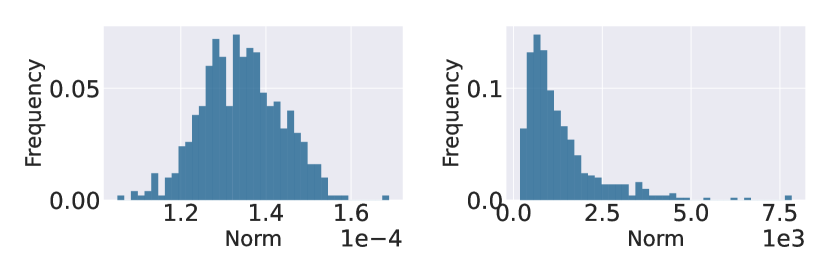
This could also be verified numerically: we compare $\|\nabla_{x}f\|_{F}$ on training data before and after training and show the histogram in Figure 1. We can see that the magnitude of $\|\nabla_{x}f\|_{F}$ grows much larger in well-trained model $w_{p}$ than randomly initialized model $w_{0}$. During the learning process, training data contribute to model performance, and such efforts include promoting model sensitivity to them. Thereby, we use $df/dx$ as an estimation for sample contribution $d{\cal A}/d{\mathcal{X}}$ .

Figure 1: Input sensitivity $\|\nabla_{x}f\|_{F}$ of training data before and after training. Left: In randomly initialized model $w_{0}$. Right: In well-trained model $w_{p}$. The learning process largely increases the sensitivity.

Figure 2: Input sensitivity $\|\nabla_{x}f_{c}\|_{F}$ and $\|\nabla_{x}f_{c^{\prime}}\|_{F}$ of training data before and after training. Left: In randomly initialized model $w_{0}$. Right: In well-trained model $w_{p}$. After training, the distinction in sensitivity between different classes becomes larger, resulting in a promising discrepancy of whether a sample is involved in training or not.

3.3 Input Sensitivity in the Target and Irrelevant Class

The above findings show that input sensitivity can approximately measure the sample contribution to the learned model. This notion is further supported by the observed increasing trend of input sensitivity during the training process. During the learning process, the semantic meaning is fed via approaching the label. Consequently, the contributions of training samples to different labels vary. It could be expected that the input sensitivity for the target class is more pronounced compared to that for other irrelevant classes.

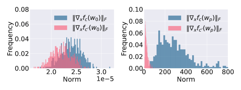
Let $f_{c}$ stand for the logit output of the target class and $f_{c^{\prime}}$ for the irrelevant classes. Figure 2 illustrates the distribution of $\|\nabla_{x}f_{c}\|_{F}$ and $\sum_{c^{\prime}\neq c}\nolimits\|\nabla_{x}f_{c^{\prime}}\|_{F}$ before and after training. For a randomly initialized model, there is little response to input changes, only about $10^{-5}$. However, after training, there is a significant order of magnitude growth in these quantities, indicating an increased attention of the trained model to input variations. As expected, these two quantities are of comparative magnitude in the randomly initialized model, but $\|\nabla_{x}f_{c}\|_{F}$ becomes much larger than $\|\nabla_{x}f_{c^{\prime}}\|_{F}$ after training. This observation implies that the model amplifies $\|\nabla_{x}f_{c}\|_{F}$ to surpass $\|\nabla_{x}f_{c^{\prime}}\|_{F}$, thereby generating a discernible difference in whether a sample has been learned.

3.4 Input Sensitivity with and without Involved in Training

Previously, we focus on the change of input sensitivity in the training process. Here, we shift to exploring input sensitivity from a sample-based perspective.

Roughly speaking, when a sample is used for training, its sensitivity should be larger than in cases where it is absent from the training set. Numerically, we inspect the forgetting data across 3 tasks studied in this paper, including unlearning a full class, sub-class, and random subset. For each instance, we compare the retrained model’s sensitivity to that of the pretrained model. Such difference serves as an approximation of the sample’s contribution to $\nabla_{x}f$, and further to the learned model. Aiming for a lightweight unlearning algorithm, we prefer an optimization direction rather than specifying a target value for each sample. Therefore, we care more about the sign of difference rather than magnitude. We calculate the difference for each forgetting instance in $\|\nabla_{x}f_{c}\|_{F},\sum_{c^{\prime}\neq c}\nolimits\|\nabla_{x}f_{c^{\prime}}\|_{F}$ between the retrained model $w_{r}$ and the pretrained model $w_{p}$, and then count the ratio of rise and fall, examining the overall trend. The result is shown in Figure 3.

Figure 3: Proportion of input sensitivity rise and fall across 3 tasks. Top: $\Delta=\|\nabla_{x}f_{c}(w_{r},x)\|_{F}-\|\nabla_{x}f_{c}(w_{p},x)\|_{F}$. Bottom: $\Delta=\sum_{c^{\prime}\neq c}\nolimits\|\nabla_{x}f_{c^{\prime}}(w_{r},x)\|_{F}-\sum_{c^{\prime}\neq c}\nolimits\|\nabla_{x}f_{c^{\prime}}(w_{p},x)\|_{F}$. Learning an instance promotes its $\|\nabla_{x}f_{c}\|_{F}$ and suppresses its $\sum_{c^{\prime}\neq c}\nolimits\|\nabla_{x}f_{c^{\prime}}\|_{F}$.

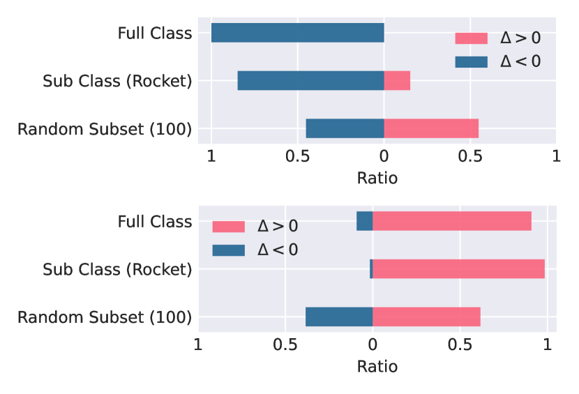
In the upper graph of Figure 3, $\Delta$ refers to $\|\nabla_{x}f_{c}(w_{r},x)\|_{F}-\|\nabla_{x}f_{c}(w_{p},x)\|_{F}$. For full class and sub-class on rocket cases, where the retrained model exhibits limited generalization on the forgetting data, $f_{c}$ of the retrained model is less sensitive to most $\mathcal{D}_{f}$ than the pretrained model. It indicates that if the model can successfully classify these instances, $f_{c}$ will exhibit a more pronounced response to changes in their input. For random subset cases, where the retrained model still has considerable generalization on the forgetting data, there is no obvious trend across $\mathcal{D}_{f}$. Therefore, we conclude that $\|\nabla_{x}f_{c}\|_{F}$ is more related to correct prediction on samples.

In the lower graph of Figure 3, $\Delta$ refers to $\sum_{c^{\prime}\neq c}\|\nabla_{x}f_{c^{\prime}}(w_{r},x)\|_{F}-\sum_{c^{\prime}\neq c}\|\nabla_{x}f_{c^{\prime}}(w_{p},x)\|_{F}$. Across 3 tasks, $\sum_{c^{\prime}}\|\nabla_{x}f_{c^{\prime}}\|_{F}$ of samples are consistently smaller in the pretrained model than that in the retrained model. It implies that if a sample is in the training set, its $\sum_{c^{\prime}\neq c}\|\nabla_{x}f_{c^{\prime}}\|_{F}$ may be implicitly regularized during training. Therefore, for each instance, $\sum_{c^{\prime}\neq c}\|\nabla_{x}f_{c^{\prime}}\|_{F}$ correlates more with whether it is seen by the model during training.

3.5 Unlearning by Suppressing Relative Magnitude

The difference in sensitivity change trend suggests that unlearning cannot purely minimize $\|\nabla_{x}f\|_{F}$ but should take the inherent difference into account. Since the changes occur in opposite directions, the simplest choice is to consider the relative magnitude $\|\nabla_{x}f_{c}\|_{F}-\sum_{c^{\prime}\neq c}\|\nabla_{x}f_{c^{\prime}}\|_{F}$, regardless of their relative weight.

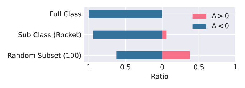
To support our idea, we investigate the relative magnitude across 3 tasks. Comparing the ratios in Figure 4 with those in Figure 3, we observe a higher proportion of magnitude decrease. This can be attributed to the accumulation of differences in $\|\nabla_{x}f_{c}\|_{F}$ and $\sum_{c^{\prime}\neq c}\|\nabla_{x}f_{c^{\prime}}\|_{F}$ within the relative magnitude, leading to more pronounced decreases. Therefore, the sample contribution to the model manifests in promoting $f_{c}$’s response to input changes and meanwhile suppressing the reaction of irrelevant classes $f_{c^{\prime}}$.

Figure 4: Proportion of relative magnitude rise and fall across 3 tasks. $\Delta=R(w_{r})-R(w_{p})$, where $R=\|\nabla_{x}f_{c}(w,x)\|_{F}-\sum_{c^{\prime}\neq c}\|\nabla_{x}f_{c^{\prime}}(w,x)\|_{F}$. There is a more consistent trend in the change of the relative magnitude $R$, which means a sample’s contribution to training lies in enhancing its relative magnitude $R$.

The relative magnitude includes both class-wise level and instance-wise level behavior. This is in line with unlearning, which requires wiping off both the public (shared within the class) and the private (unique to the instance) information that an instance contributes. Based upon the above insights, we propose to unlearning by rolling back such an enhancement on relative magnitude. Minimizing this loss guides the well-trained model to roll back $\|\nabla f_{c}\|_{F}$ and pick up $\|\nabla f_{c^{\prime}}\|_{F}$. Mathematically, our optimization objective is expressed as:

$$\min\limits_{w}\sum_{x\in\mathcal{D}_{f}}\underbrace{\|\nabla_{x}f_{c}(w,x)\|^{2}_{F}-\|\nabla_{x}f_{c^{\prime}}(w,x)\|^{2}_{F}}_{=:\mathcal{L}(w,x)}$$ (1)

where $c$ is target label and $c^{\prime}\neq c$ are the irrelevant labels.

Our overall algorithm is given in Algorithm 1, which has the pretrained model and forgetting data as input and has three hyperparameters, namely, the step length $\eta$, the max iterations $T_{MU}$, and a stopping threshold $\delta$. $\delta$ controls change of relative magnitude. For MU-Mis, $\delta$ is a particular parameter and its value depends on a specific unlearning task. Generally, a large $\delta$ means that we require significant change on $\mathcal{L}$, which is suitable for full class and sub-class unlearning. For random sample unlearning, there will be a slight difference from the pretrained model, and so $\delta$ is suggested to be small.

Algorithm 1 MU-Mis: Machine Unlearning via Minimizing Input Sensitivity

  Input: Pretrained model $w_{p}$, forgetting data $\mathcal{D}_{f}$, step length $\eta$, stopping threshold $\delta$, max iterations $T_{MU}$

  Output: Unlearned model $w_{u}$

  Initialize model parameters $w_{0}=w_{p}$

  Measure initial loss $\tilde{\mathcal{L}}_{0}=\sum_{x\in\mathcal{D}_{f}}\mathcal{L}(w_{0},x)$ in (1)

  repeat

     for $t=0$ to $T_{MU}-1$ do

        Initialize $\Delta w=0$.

        Initialize avgerage loss $\tilde{\mathcal{L}}=0$.

        for $x\in\mathcal{D}_{f}$ do

           Randomly select a random irrelevant class $c^{\prime}\neq c$

           Compute $\mathcal{L}(w_{t},x)$

           $\Delta w=\Delta w+\nabla_{w}\mathcal{L}(w_{t},x)$

        end for

        $w_{t+1}=w_{t}-\eta\Delta w$

        $\Delta\tilde{\mathcal{L}}=\dfrac{1}{|\mathcal{D}_{f}|}(\tilde{\mathcal{L}}_{0}-\tilde{\mathcal{L}})$

     end for

  until $\Delta\tilde{\mathcal{L}}\geq\delta$

4 Experiment

4.1 Setup

Unlearning Tasks. We investigate 3 kinds of unlearning tasks in supervised image classification scenarios, including forgetting a full class, a sub-class under a super-class, and a random subset. Three tasks are respectively evaluated with CIFAR-100, CIFAR-20, and CIFAR-10 in line with (Golatkar et al., 2020a; Foster et al., 2023). Specifically, we perform full class unlearning by forgetting the “Rocket” class, subclass unlearning by forgetting the “Rocket” and “Sea” classes, and random subset unlearning by randomly selecting 100 samples. For a more comprehensive evaluation, we pick “Rocket” and “Sea” two cases in subclass unlearning, corresponding to cases the retrained model generalizes on the forgetting data or not. Following Foster et al. (2023), we also evaluate full class unlearning on Face Recognition classification, with PinsFaceRecognition (Burak, 2020) dataset consisting of 17,534 faces of 105 celebrities.

Evaluation Metrics. Machine unlearning algorithms should be assessed based on three aspects: utility, privacy, and efficiency. For utility evaluation, we evaluate the accuracy of the forgetting data and the remaining data. For privacy guarantee, we use membership inference attack (MIA) to evaluate information remaining after unlearning. Notice that MIA itself is an interesting and developing field. Thus, although we select a very good MIA method (Chundawat et al., 2023), it still may confuse unseen data as the training set. Additionally, we also compare the execution time with other methods to measure timeliness.

Baselines. We evaluate our method along with 5 unlearning methods, including finetuning on the remaining data, blindspot (Chundawat et al., 2023) which transfers knowledge from useful and useless teachers, amnesiac (Graves et al., 2021) which records and withdraws related historical updates, Boundary Shrink which shifts the decision boundary and SSD (Foster et al., 2023) which suppresses specialized parameter for the forgetting data. Among them, Boundary Shrink is designed for full class unlearning and thus omitted in the other 2 tasks. It is worth noting that the above baselines, except for Boundary Shrink, all require utilizing the remaining data.

Implementations. Our method and baselines are implemented with PyTorch and conducted on NVIDIA GeForce RTX 2080Ti. We train our ResNet18 (He et al., 2016) model from scratch for 200 epochs in line with (Foster et al., 2023). The step length is chosen from $\{10^{-3},2\times 10^{-3},5\times 10^{-3}\}$. $T_{MU}$ is set to 30 in all experiments .

4.2 Unlearning Performance

Full Class Unlearn Table 1 and Table 2 show the performance of full class unlearning on “Rocket” in CIFAR100 and PinsFaceRecognition. On both datasets, MU-Mis effectively scrubs information of the forgetting class while preserving the highest accuracy on the remaining data.

Table 1: Full class unlearning on CIFAR-100 with ResNet18.

Methods	Retain Acc	Forget Acc	MIA
Pretrain	76.36	86.02	95.40
Finetune	64.91	0.00	12.00
Blindspot	74.82	0.00	0.00
Amnesiac	73.84	0.00	27.40
Bound. Shrink	62.37	0.00	9.40
SSD	76.06	0.00	0.00
MU-Mis	76.32	0.00	0.00
Retrain	76.91	0.00	5.60

Table 2: Full class unlearning on PinsFaceRecognition with ResNet18.

Methods	Retain Acc	Forget Acc	MIA
Pretrain	100.0	100.0	100.0
Finetune	89.45	0.00	2.35
Blindspot	92.23	0.00	0.00
Amnesiac	91.40	0.00	87.05
Bound. Shrink	88.73	4.71	0.00
SSD	86.85	0.00	0.00
MU-Mis	92.83	0.00	0.00
Retrain	92.43	0.00	0.00

Sub-Class Unlearn Table 3 and Table 4 present the performance of sub-class unlearning. “Rocket” and “Sea” correspond to two cases of sub-class unlearning, with distinction in whether the retrained model can generalize to the forgetting class. In both cases, MU-Mis is closest to the retrained model on the accuracy of the remaining and forgetting data. For MIA, the value is the ratio of forgetting data that are recognized as the training data by Chundawat et al. (2023). Thus, a lower value is desired. However, for the two sub-class unlearn tasks, the value for the retrained model is not low, which is due to the imperfections of the current MIA method. In this case, the reported MIA values are only for reference.

Table 3: Sub-class (Rocket) unlearning on CIFAR-20 with ResNet18.

Methods	Retain Acc	Forget Acc	MIA
Pretrain	85.26	80.73	92.80
Finetune	73.60	2.95	11.60
Blindspot	83.71	1.39	0.00
Amnesiac	81.90	1.39	13.60
SSD	75.29	0.00	16.00
MU-Mis	83.81	2.17	0.60
Retrain	84.95	2.95	12.40

Table 4: Sub-class (Sea) unlearning on CIFAR-20 with ResNet18.

Methods	Retain Acc	Forget Acc	MIA
Pretrain	85.09	97.66	91.80
Finetune	74.42	72.40	51.00
Blindspot	83.50	78.56	0.00
Amnesiac	81.90	30.73	13.60
SSD	81.55	0.00	1.80
MU-Mis	85.01	97.66	83.40
Retrain	84.00	97.05	95.40

Table 5: Random subset unlearning on CIFAR-10 with ResNet18.

Methods	Retain Acc	Forget Acc	MIA
Pretrain	94.67	100.0	95.00
Finetune	89.99	94.00	79.00
Blindspot	94.17	91.00	34.00
Amnesiac	93.16	28.00	16.00
SSD	94.67	100.0	93.00
MU-Mis	94.67	100.0	94.00
Retrain	94.79	100.0	94.00

Random Subset Unlearn Table 5 displays the performance of random subset unlearning. There is a clear gap between other methods and retraining except for SSD and MU-Mis.

4.3 Time Consuming Comparison

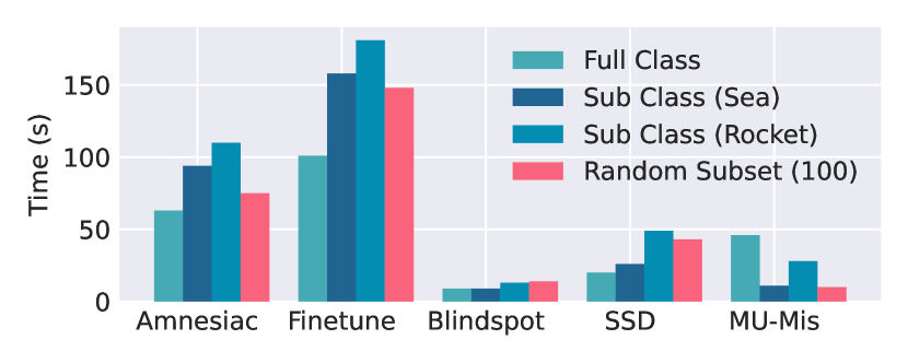
We compared the unlearning time of different methods for three unlearn tasks, referred to Figure 5. MU-Mis is approximately $1000\times/100\times/100\times/80\times$ times faster than retraining in full class / sub-class (Rocket) / sub-class (Sea) / random subset tasks. The time consumption of retraining is omitted in the figure for the substantial difference in orders of magnitude compared to the other methods.

Our method along with blindspot and SSD are overall more efficient than others. For unlearning a single class, blindspot is the fastest, and our method is comparable to SSD. When it comes to forgetting a random subset, our method is faster than the others.

Figure 5: Time consumption of different unlearning methods. Our method is quite effective.

4.4 Attention Map

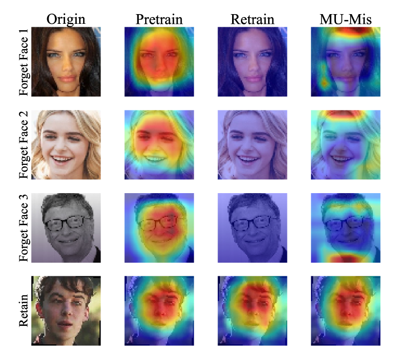
To further investigate and understand the behavior of our unlearned model, we examine the attention heatmaps of the models before and after applying our unlearning method to the data for PinsFaceRecognition, as shown in Figure 6. Attention heatmaps (Selvaraju et al., 2017) are widely used to highlight important regions in an image that contribute to prediction. For the forgetting data, the original attention is focused on the faces. After applying MU-Mis, the attention on the faces either disappears or significantly weakens, and is shifted towards the background at the image edges (last column in the first three rows of Figure 6). For the remaining data, MU-Mis fully maintains attention (last column in the last row of Figure 6). Importantly, an alternative interpretation of input sensitivity is the measurement of how changes in an image influence its model prediction (Smilkov et al., 2017). Our proposed method effectively reduces the sensitivity to the forgetting data class by suppressing $\|\nabla f_{c}\|_{F}$, while enhancing $\|\nabla f_{c^{\prime}}\|_{F}$ to prevent sensitivity degradation in the retain classes. These results demonstrate that MU-Mis enables the unlearned model to disregard the semantic information in the forgotten data while preserving prediction sensitivity and performance on the remaining data.

Figure 6: Visualization of attention maps for the full class unlearning task on PinsFaceRecognition. From left to right: original image, pretrained model attention, retrained model attention, and unlearned model attention by MU-Mis. The first three rows show the results of different methods when forgetting a single class. The last row displays the results of different methods on the remaining data. MU-Mis successfully distracts the model’s attention from the forgetting data’s semantic region while preserving the remaining data.

4.5 Ablation Study

We study the role of each term in our loss (1) by taking the full class (Rocket) unlearning as an example. We denote the first term $\|\nabla_{x}f_{c}(w,x)\|^{2}_{F}$ in our loss as TC (Target Class) and the second term $\|\nabla_{x}f_{c^{\prime}}(w,x)\|^{2}_{F}$ as OC (Other Class). In Table 6, we present the unlearning performance of decreasing TC, increasing OC, and decreasing TC - OC, respectively. We set an upper bound for OC to avoid performance breakdown. Learning from the ablation study, we observe that minimizing the first term obliviates information of the forgetting data, but greatly hurts performance on the remaining data. Solely increasing OC brings a slight accuracy drop on remaining data, and hardly affects the forgetting data. We further investigate whether the second term takes effect only when $\|\nabla_{x}f_{c}\|^{2}_{F}$ is small enough. We decrease TC at first and then switch to increasing OC when the accuracy on the forgetting data drops to 0, denoting it as TC, OC. As expected, the accuracy of the remaining data stages a recovery compared to TC only.

Table 6: Ablation study on each term of our loss in full class (Rocket) unlearning. TC (Target Class) refers to the first term and OC (Other Class) refers to the second term.

Methods	Retain Acc	Forget Acc	MIA
Pretrain	76.36	86.02	95.40
TC	60.45	0.00	5.80
OC	75.58	86.02	96.40
TC, OC	71.55	8.51	0.20
TC - OC	76.32	0.00	0.00
Retrain	76.91	0.00	5.60

5 Conclusion

From the fact that sample contribution to the learning process is a key difference for whether the data are involved in the training or not, we in this paper propose a novel method to suppress sample contribution for machine unlearning. Via analysis, we find that sample contribution reflects on the input sensitivity of the learned model, which can be efficiently calculated and optimized. Based on this, MU-Mis is designed and evaluated on standard unlearning tasks and comparison with SOTA methods. The empirical results illustrate that sample contribution could be promising for investigating learning and unlearning behavior.

MU-Mis hardly disturbs performance on the remaining data and we empirically discuss the orthogonality across samples in Appendix A. But the reason behind is not well-understood. Another limitation is how to better measure sample contribution. Input sensitivity is only an approximation. More in-depth analyses are needed to achieve better unlearning. Especially, the use of learning dynamic trajectory is needed.

6 Boarder Impacts

Our research establishes a connection between input sensitivity and sample contribution, providing a novel perspective for MU from the sample level. We also propose an efficient and effective loss function that is designed to suppress sample contributions and forget any training data point by minimizing relative magnitudes. Although not discussed in this paper, our viewpoints and proposed methods may have implications in areas such as protecting model privacy, mitigating bias or toxic data, enhancing model robustness, and improving generalization capabilities.

Appendix A Additional Discussion

One great advantage of our method is that we don’t need the remaining data. In this part, we demonstrate such an advantage by showing the inherent orthogonality from the perspective of input sensitivity. And we empirically demonstrate that optimizing our proposed loss function solely on the forgetting data does not affect the relative magnitudes of input sensitivities for the remaining data.

A.1 Input Sensitivity More Orthogonal than Output-based Derivatives

Current gradient-based unlearning methods (Wu et al., 2020; Graves et al., 2021; Neel et al., 2021) utilize loss gradient $\nabla_{\theta}\mathcal{L}(w,x)$ to reverse parameter updates of the forgetting data, where $\mathcal{L}$ refers to cross-entropy loss. However, gradients are quite similar within a class in a well-trained model (Fort & Ganguli, 2019; Papyan, 2020). To avoid performance drop on the remaining data, previous work relies on utilizing the remaining data to patch up the damage (Tarun et al., 2023) or introduce extra maintenance (Fan et al., 2023; Hoang et al., 2024). Different from previous methods, we leverage the model’s sensitivity to input instead of directly computing derivatives from output w.r.t. parameters. We show that manipulations based on input sensitivity exhibit greater orthogonality between samples, even within the same class

We calculate the pairwise cosine similarity within a class and between classes of the derivatives of four metrics w.r.t. parameters in a well-trained model. They are $\nabla_{w}\mathcal{L},\nabla_{w}f_{c},\nabla_{w}\|\nabla_{x}f_{c}\|_{F},$ and $\nabla_{w}\sum_{c^{\prime}\neq c}\|\nabla_{x}f_{c^{\prime}}\|_{F}$. The first two metrics are commonly used in current unlearning methods, and the last two are utilized in our proposed approach. The similarity results are shown in Figure 7. Derivatives of all four metrics are approximately orthogonal between samples from different classes. However, intra-class similarities differ across four metrics. We can see that both $\nabla_{w}\mathcal{L}$ and $\nabla_{w}f_{c}$ bear a resemblance within a class, with cosine similarity centering around $0.3$ and reaching up to $0.6$. On the other hand, $\nabla_{w}\|\nabla_{x}f_{c}\|_{F}$ centers around $0.1$ with intra-class similarity scarcely exceeding $0.3$. Directly taking the derivative of output w.r.t parameters preserves within-class similarity of the output, but such similarity is reduced when output first takes the derivative to the input and then back to parameters.

Interestingly, $\nabla_{w}\sum_{c^{\prime}\neq c}\|\nabla_{x}f_{c^{\prime}}\|_{F}$ seems to be pairwise similar. However, we speculate that there are two reasons why this portion of our loss function does not significantly harm the performance of the remaining data. Firstly, as shown in Figure 2, $\sum_{c^{\prime}\neq c}\|\nabla_{x}f_{c^{\prime}}\|_{F}$ is significantly smaller than $\|\nabla_{x}f_{c}\|_{F}$ on well-trained models. Therefore, in the early stages of optimizing the relative magnitudes of input sensitivities, the contribution of $\nabla_{w}\sum_{c^{\prime}\neq c}\|\nabla_{x}f_{c^{\prime}}\|_{F}$ to the optimization direction can be neglected. Secondly, $\sum_{c^{\prime}\neq c}\|\nabla_{x}f_{c^{\prime}}\|_{F}$ for the forgetting data actually corresponds to the target class of some remaining data. The inter-class similarity of $\nabla_{w}\sum_{c^{\prime}\neq c}\|\nabla_{x}f_{c^{\prime}}\|_{F}$ implies that when we increase the input sensitivity of the forgetting data for the other irrelevant classes, we also increase the input sensitivity of the remaining data of the corresponding classes, thus preserving their sample contributions.

Figure 7: Inter-class and intra-class cosine similarity of four different metrics w.r.t parameters. From left to right: $\nabla_{w}\mathcal{L}$, $\nabla_{w}f_{c}$, $\nabla_{w}\|\nabla_{x}f_{c}\|_{F}$, and $\nabla_{w}\|\nabla_{x}f_{c^{\prime}}\|_{F}$. Directly taking the derivative of output w.r.t parameters bears a resemblance across samples, but such similarity is reduced when output first takes derivative to input and then back to parameters.

A.2 Relative Magnitudes of The Remaining Data Keeping Stable

Figure 8: The relative magnitudes of input sensitivities between the forgetting and remaining data during the unlearning process.

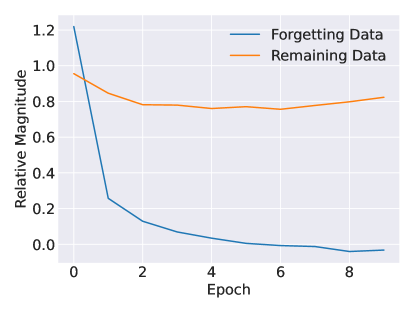
To investigate the impact of applying our proposed loss function solely on the forgetting data on the remaining data, we examined the changes in the relative magnitudes of input sensitivities between the forgotten and retained data during the unlearning process. The results in Figure 8 indicate that as we minimize our loss function on the forgetting data to eliminate their contribution to the model, the relative magnitudes on the remaining data only slightly decrease and keep nearly unchanged throughout the unlearning process. As analyzed in the above part, this can be attributed to the inherent orthogonality of $\nabla_{w}\|\nabla_{x}f_{c}\|_{F}$ among samples and the negligible contribution of $\nabla_{w}\sum_{c^{\prime}\neq c}\|\nabla_{x}f_{c^{\prime}}\|_{F}$ to the optimization, which ensures that the performance on the remaining data is preserved during the unlearning process.

References

- Achille et al. (2019) Achille, A., Paolini, G., and Soatto, S. Where is the information in a deep neural network? arXiv preprint arXiv:1905.12213, 2019.
- Basu et al. (2020) Basu, S., Pope, P., and Feizi, S. Influence functions in deep learning are fragile. In International Conference on Learning Representations, 2020.
- Burak (2020) Burak. Pinterest face recognition dataset. www.kaggle.com/datasets/hereisburak/pins-facerecognition, 2020.
- Cao & Yang (2015) Cao, Y. and Yang, J. Towards making systems forget with machine unlearning. In IEEE Symposium on Security and Privacy, pp. 463–480. IEEE, 2015.
- Christmann & Steinwart (2008) Christmann, A. and Steinwart, I. Support Vector Machines. Springer, 2008.
- Chundawat et al. (2023) Chundawat, V. S., Tarun, A. K., Mandal, M., and Kankanhalli, M. Can bad teaching induce forgetting? unlearning in deep networks using an incompetent teacher. In the AAAI Conference on Artificial Intelligence, pp. 7210–7217, 2023.
- Cortes & Vapnik (1995) Cortes, C. and Vapnik, V. Support-vector networks. Machine Learning, 20:273–297, 1995.
- Fan et al. (2023) Fan, C., Liu, J., Zhang, Y., Wei, D., Wong, E., and Liu, S. Salun: Empowering machine unlearning via gradient-based weight saliency in both image classification and generation. arXiv preprint arXiv:2310.12508, 2023.
- Feldman (2020) Feldman, V. Does learning require memorization? a short tale about a long tail. In the Annual ACM SIGACT Symposium on Theory of Computing, pp. 954–959, 2020.
- Feldman & Zhang (2020) Feldman, V. and Zhang, C. What neural networks memorize and why: Discovering the long tail via influence estimation. Advances in Neural Information Processing Systems, 33:2881–2891, 2020.
- Fort & Ganguli (2019) Fort, S. and Ganguli, S. Emergent properties of the local geometry of neural loss landscapes. arXiv preprint arXiv:1910.05929, 2019.
- Foster et al. (2023) Foster, J., Schoepf, S., and Brintrup, A. Fast machine unlearning without retraining through selective synaptic dampening. arXiv preprint arXiv:2308.07707, 2023.
- Golatkar et al. (2020a) Golatkar, A., Achille, A., and Soatto, S. Eternal sunshine of the spotless net: Selective forgetting in deep networks. In IEEE/CVF Conference on Computer Vision and Pattern Recognition, pp. 9304–9312, 2020a.
- Golatkar et al. (2020b) Golatkar, A., Achille, A., and Soatto, S. Forgetting outside the box: Scrubbing deep networks of information accessible from input-output observations. In European Conference on Computer Vision, pp. 383–398, 2020b.
- Graves et al. (2021) Graves, L., Nagisetty, V., and Ganesh, V. Amnesiac machine learning. In the AAAI Conference on Artificial Intelligence, pp. 11516–11524, 2021.
- Guo et al. (2020) Guo, C., Goldstein, T., Hannun, A. Y., and van der Maaten, L. Certified data removal from machine learning models. In Proceedings of the 37th International Conference on Machine Learning, pp. 3832–3842, 2020.
- He et al. (2016) He, K., Zhang, X., Ren, S., and Sun, J. Deep residual learning for image recognition. In IEEE Conference on Computer Vision and Pattern Recognition, pp. 770–778, 2016.
- Hoang et al. (2024) Hoang, T., Rana, S., Gupta, S., and Venkatesh, S. Learn to unlearn for deep neural networks: Minimizing unlearning interference with gradient projection. In IEEE/CVF Winter Conference on Applications of Computer Vision, pp. 4819–4828, 2024.
- Koh & Liang (2017) Koh, P. W. and Liang, P. Understanding black-box predictions via influence functions. In International Conference on Machine Learning, pp. 1885–1894. PMLR, 2017.
- Mehta et al. (2022) Mehta, R., Pal, S., Singh, V., and Ravi, S. N. Deep unlearning via randomized conditionally independent hessians. In IEEE/CVF Conference on Computer Vision and Pattern Recognition, pp. 10422–10431, 2022.
- Neel et al. (2021) Neel, S., Roth, A., and Sharifi-Malvajerdi, S. Descent-to-delete: Gradient-based methods for machine unlearning. In Algorithmic Learning Theory, pp. 931–962. PMLR, 2021.
- Papyan (2020) Papyan, V. Traces of class/cross-class structure pervade deep learning spectra. Journal of Machine Learning Research, 21(1):10197–10260, 2020.
- Peste et al. (2021) Peste, A., Alistarh, D., and Lampert, C. H. SSSE: Efficiently erasing samples from trained machine learning models. In NeurIPS 2021 Workshop Privacy in Machine Learning, 2021.
- Regulation (2018) Regulation, G. D. P. General data protection regulation (GDPR). Intersoft Consulting, Accessed in October, 24(1), 2018.
- Selvaraju et al. (2017) Selvaraju, R. R., Cogswell, M., Das, A., Vedantam, R., Parikh, D., and Batra, D. Grad-cam: Visual explanations from deep networks via gradient-based localization. In IEEE International Conference on Computer Vision, pp. 618–626, 2017.
- Shokri et al. (2017) Shokri, R., Stronati, M., Song, C., and Shmatikov, V. Membership inference attacks against machine learning models. In 2017 IEEE Symposium on Security and Privacy (SP), pp. 3–18. IEEE, 2017.
- Smilkov et al. (2017) Smilkov, D., Thorat, N., Kim, B., Viégas, F., and Wattenberg, M. Smoothgrad: removing noise by adding noise. arXiv preprint arXiv:1706.03825, 2017.
- Suriyakumar & Wilson (2022) Suriyakumar, V. and Wilson, A. C. Algorithms that approximate data removal: New results and limitations. Advances in Neural Information Processing Systems, pp. 18892–18903, 2022.
- Tarun et al. (2023) Tarun, A. K., Chundawat, V. S., Mandal, M., and Kankanhalli, M. Fast yet effective machine unlearning. IEEE Transactions on Neural Networks and Learning Systems, 2023.
- Wu et al. (2022) Wu, G., Hashemi, M., and Srinivasa, C. Puma: Performance unchanged model augmentation for training data removal. In the AAAI Conference on Artificial Intelligence, volume 36, pp. 8675–8682, 2022.
- Wu et al. (2020) Wu, Y., Dobriban, E., and Davidson, S. Deltagrad: Rapid retraining of machine learning models. In International Conference on Machine Learning, pp. 10355–10366. PMLR, 2020.
- Xu et al. (2023) Xu, J., Wu, Z., Wang, C., and Jia, X. Machine unlearning: Solutions and challenges. arXiv preprint arXiv:2308.07061, 2023.
- Zhang et al. (2021) Zhang, C., Ippolito, D., Lee, K., Jagielski, M., Tramèr, F., and Carlini, N. Counterfactual memorization in neural language models. arXiv preprint arXiv:2112.12938, 2021.
- Zhu et al. (2019) Zhu, L., Liu, Z., and Han, S. Deep leakage from gradients. Advances in Neural Information Processing Systems, 32, 2019.