Error Feedback Reloaded: From Quadratic to Arithmetic Mean of Smoothness Constants
Abstract
Error Feedback (EF) is a highly popular and immensely effective mechanism for fixing convergence issues which arise in distributed training methods (such as distributed GD or SGD) when these are enhanced with greedy communication compression techniques such as TopK. While EF was proposed almost a decade ago (Seide et al., 2014), and despite concentrated effort by the community to advance the theoretical understanding of this mechanism, there is still a lot to explore. In this work we study a modern form of error feedback called EF21 (Richtárik et al., 2021) which offers the currently best-known theoretical guarantees, under the weakest assumptions, and also works well in practice. In particular, while the theoretical communication complexity of EF21 depends on the quadratic mean of certain smoothness parameters, we improve this dependence to their arithmetic mean, which is always smaller, and can be substantially smaller, especially in heterogeneous data regimes. We take the reader on a journey of our discovery process. Starting with the idea of applying EF21 to an equivalent reformulation of the underlying problem which (unfortunately) requires (often impractical) machine cloning, we continue to the discovery of a new weighted version of EF21 which can (fortunately) be executed without any cloning, and finally circle back to an improved analysis of the original EF21 method. While this development applies to the simplest form of EF21, our approach naturally extends to more elaborate variants involving stochastic gradients and partial participation. Further, our technique improves the best-known theory of EF21 in the rare features regime (Richtárik et al., 2023). Finally, we validate our theoretical findings with suitable experiments.
1 Introduction
Due to their ability to harness the computational capabilities of modern devices and their capacity to extract value from the enormous data generated by organizations, individuals, and various digital devices and sensors, Machine Learning (ML) methods (Bishop, 2016; Shalev-Shwartz & Ben-David, 2014) have become indispensable in numerous practical applications (Krizhevsky et al., 2012; Lin et al., 2022; Vaswani et al., 2017; Onay & Öztürk, 2018; Poplin et al., 2017; Gavriluţ et al., 2009; Sun et al., 2017).
The necessity to handle large datasets has driven application entities to store and process their data in powerful computing centers (Yang et al., 2019; Dean et al., 2012; Verbraeken et al., 2020) via distributed training algorithms. Beside this industry-standard centralized approach, decentralized forms of distributed learning are becoming increasingly popular. For example, Federated Learning (FL) facilitates a collaborative learning process in which various clients, such as hospitals or owners of edge devices, collectively train a model on their devices while retaining their data locally, without uploading it to a centralized location (Konečný et al., 2016b; a; McMahan et al., 2017; Li et al., 2020a; Kairouz et al., 2021; Wang et al., 2021).
Distributed training problems are typically formulated as optimization problems of the form
| (1) |
where is the number of clients/workers/nodes, vector represents the trainable parameters, and is the loss of the model parameterized by on the training data stored on client . One of the key issues in distributed training in general, and FL in particular, is the communication bottleneck (Konečný et al., 2016b; Kairouz et al., 2021). The overall efficiency of a distributed algorithm for solving (1) can be characterized by multiplying the number of communication rounds needed to find a solution of acceptable accuracy by the cost of each communication round:
| (2) |
This simple formula clarifies the rationale behind two orthogonal approaches to alleviating the communication bottleneck. i) The first approach aims to minimize the first factor in (2). This is done by carefully deciding on what work should be done on the clients in each communication round in order for it to reduce the total number of communication rounds needed, and includes methods based on local training (Stich, 2018; Lin et al., 2018; Mishchenko et al., 2022; Condat et al., 2023; Li et al., 2019) and momentum (Nesterov, 1983; 2004; d’Aspremont et al., 2021). Methods in this class communicate dense -dimensional vectors. ii) The second approach aims to minimize the second factor in (2). Methods in this category compress the information (typically -dimensional vectors) transmitted between the clients and the server (Alistarh et al., 2017; Khirirat et al., 2018; Bernstein et al., 2018; Safaryan et al., 2021).
1.1 Communication compression
Vector compression can be achieved through the application of a compression operator. Below, we outline two primary classes of these operators: unbiased (with conically bounded variance) and contractive.
Definition 1 (Compressors).
A randomized mapping is called i) an unbiased compressor if for some it satisfies
| (3) |
and ii) a contractive compressor if for some it satisfies
| (4) |
It is well known that whenever a compressor satisfies (3), then the scaled compressor satisfies (4) with . In this sense, the class of contractive compressors includes all unbiased compressors as well. However, it is also strictly larger. For example, the Top compressor, which retains the largest elements in absolute value of the vector it is applied to and replaces the rest by zeros, and happens to be very powerful in practice (Alistarh et al., 2018), satisfies (4) with , but does not satisfy (3). From now on, we write to denote the class of compressors satisfying (4).
It will be convenient to define the following functions of the contraction parameter
| (5) |
Note that . The behavior of distributed algorithms utilizing unbiased compressors for solving (1) is relatively well-understood from a theoretical standpoint (Khirirat et al., 2018; Mishchenko et al., 2019; Li et al., 2020b; Gorbunov et al., 2021; Tyurin & Richtárik, 2023). By now, the community possesses a robust theoretical understanding of the advantages such methods can offer and the mechanisms behind their efficacy (Gorbunov et al., 2020; Khaled et al., 2023; Tyurin & Richtárik, 2023). However, it is well known that the class of contractive compressors includes some practically very powerful operators, such as the greedy sparsifier Top (Stich et al., 2018; Alistarh et al., 2018) and the low-rank approximator Rank (Vogels et al., 2019; Safaryan et al., 2022), which are biased, and hence their behavior is not explainable by the above developments. These compressors have demonstrated surprisingly effective performance in practice (Seide et al., 2014; Alistarh et al., 2018), even when compared to the best results we can get with unbiased compressors (Szlendak et al., 2022), and are indispensable on difficult tasks such as the fine-tuning of foundation models in a geographically distributed manner over slow networks (Wang et al., 2023).
However, our theoretical understanding of algorithms based on contractive compressors in general, and these powerful biased compressors in particular, is very weak. Indeed, while the SOTA theory involving unbiased compressors offers significant and often several-degrees-of-magnitude improvements over the baseline methods that do not use compression (Mishchenko et al., 2019; Horváth et al., 2019b; Li et al., 2020b; Gorbunov et al., 2020; 2021; Tyurin & Richtárik, 2023), the best theory we currently have for methods that can provably work with contractive compressors, i.e., the theory behind the error feedback method called EF21 developed by Richtárik et al. (2021) (see Algorithm 1) and its variants (Fatkhullin et al., 2021; Condat et al., 2022; Fatkhullin et al., 2023), merely matches the communication complexity of the underlying methods that do not use any compression (Szlendak et al., 2022).
To the best of our knowledge, the only exception to this is the very recent work of Richtárik et al. (2023) showing that in a rare features regime, the EF21 method (Richtárik et al., 2021) outperforms gradient descent (which is a special case of EF21 when for all and ) in theory. However, Richtárik et al. (2023) obtain no improvements upon the current best theoretical result for vanilla EF21 (Richtárik et al., 2021) in the general smooth nonconvex regime, outlined in Section 1.2, we investigate in this work.
1.2 Assumptions
We adopt the same very weak assumptions as those used by Richtárik et al. (2021) in their analysis of EF21.
Assumption 1.
The function is -smooth, i.e., there exists such that
| (6) |
Assumption 2.
The functions are -smooth, i.e., for all there exists such that
| (7) |
Note that if (7) holds, then (6) holds, and . So, Assumption 1 does not further limit the class of functions already covered by Assumption 2. Indeed, it merely provides a new parameter better characterizing the smoothness of than the estimate obtainable from Assumption 2 could.
Since our goal in (1) is to minimize , the below assumption is necessary for the problem to be meaningful.
Assumption 3.
There exists such that .
1.3 Summary of contributions
In our work we improve the current SOTA theoretical communication complexity guarantees for distributed algorithms that work with contractive compressors in general, and empirically powerful biased compressors such as Top and Rank in particular (Richtárik et al., 2021; Fatkhullin et al., 2021).
In particular, under Assumptions 1–3, the best known guarantees were obtained by Richtárik et al. (2021) for the EF21 method: to find a (random) vector satisfying , Algorithm 1 requires
iterations, where is the Quadratic Mean of the smoothness constants . Our main finding is an improvement of this result to
| (8) |
where is the Arithmetic Mean of the smoothness constants . We obtain this improvement in three different ways:
- i)
- ii)
- iii)
We obtain refined linear convergence results cases under the Polyak-Łojasiewicz condition. Further, our analysis technique extends to many variants of EF21, including EF21-SGD which uses stochastic gradients instead of gradients (Section E), and EF21-PP which enables partial participation of clients (Section G). Our analysis also improves upon the results of Richtárik et al. (2023) who study EF21 in the rare features regime (Section H). Finally, we validate our theory with suitable computational experiments (Sections 3, I and J).
2 EF21 Reloaded: Our Discovery Story
We now take the reader along on a ride of our discovery process.
2.1 Step 1: Cloning the client with the worse smoothness constant
The starting point of our journey is a simple observation described in the following example.
Example 1.
Let and . Assume the smoothness constants of are equal to 1, and is equal to . In this case,EF21 needs to run for
iterations. Now, envision the existence of an additional machine capable of downloading the data from the fourth “problematic” machine. By rescaling local loss functions, we maintain the overall loss function as:
Rescaling of the functions modifies the smoothness constants to for , and for . EF21, launched on this setting of five nodes, requires
iterations, where is the quadratic mean of the new smoothness constants .
This simple observation highlights that the addition of just one more client significantly enhances the convergence rate. Indeed, EF21 requires approximately fewer iterations. We will generalize this client cloning idea in the next section.
2.2 Step 2: Generalizing the cloning idea
We will now take the above motivating example further, allowing each client to be cloned arbitrarily many () times. Let us see where this gets us. For each , let denote a positive integer. We define (the total number of clients after cloning), and observe that can be equivalently written as
| (9) |
where for all and Notice that we scaled the functions as before, and that is -smooth, where .
Analysis of the convergence rate. The performance of EF21, when applied to the problem (9) involving clients, depends on the quadratic mean of the new smoothness constants:
| (10) |
Note that if for all , then .
Optimal choice of cloning frequencies. Our goal is to find integer values minimizing the function defined in (10). While we do not have a closed-form formula for the global minimizer, we are able to explicitly find a solution that is at most times worse than the optimal one in terms of the objective value. In particular, if we let for all , then
and moreover, . That is, we need at most double the number of clients in our client cloning construction. See Lemma 2 in the Appendix for details.
By directly applying EF21 theory from (Richtárik et al., 2021) to problem (9) involving clients, we obtain the advertised improvement from to .
Theorem 2 (Convergence of EF21 applied to problem (9) with machines).
When we choose the largest allowed stepsize and for all , this leads to the complexity (8); that is, by cloning client machines, we can replace in the standard rate with . A similar result can be obtained even if we do not ignore the integrality constraint, but we do not include it for brevity reasons. However, it is important to note that the cloning approach has several straightforward shortcomings, which we will address in the next section.111 In our work, we address an optimization problem of the form where represent certain constants. This formulation bears a resemblance to the meta problem in the importance sampling strategy discussed in (Zhao & Zhang, 2015). Despite the apparent similarities in the abstract formulation, our approach and the one in the referenced work diverge significantly in both motivation and implementation. While Zhao & Zhang (2015) applies importance sampling to reduce the variance of a stochastic gradient estimator by adjusting sampling probabilities, our method involves adjusting client cloning weights without sampling. Furthermore, our gradient estimator is biased, unlike the unbiased estimator in the referenced paper, and we aim to minimize the quadratic mean of the smoothness constants, which is inherently different from the objectives in Zhao & Zhang (2015). Although both approaches can be expressed through a similar mathematical framework, they are employed in vastly different contexts, and any parallelism may be coincidental rather than indicative of a direct connection.
2.3 Step 3: From client cloning to update weighting
It is evident that employing client cloning improves the convergence rate. Nevertheless, there are obvious drawbacks associated with this approach. Firstly, it necessitates a larger number of computational devices, rendering its implementation less appealing from a resource allocation perspective. Secondly, the utilization of EF21 with cloned machines results in a departure from the principles of Federated Learning, as it inherently compromises user privacy – transferring data from one device to another is prohibited in FL.
However, a simpler approach to implementing the cloning idea emerges when we assume the compressors used to be deterministic. To illustrate this, let us initially examine how we would typically implement EF21 with cloned machines:
| (11) | |||
| (12) |
We will now rewrite the same method in a different way. Assume we choose for all . We show by induction that is the same for all . We have just seen that this holds for . Assume this holds for some . Then since for all combined with the induction hypothesis, (12) and the determinism of , we see that is the same for all . Let us define for all . This is a valid definition since we have shown that does not depend on . Because of all of the above, iterations (11)–(12) can be equivalently written in the form
| (13) | |||
| (14) |
where . This transformation effectively enables us to operate the method on the original clients, eliminating the need for clients! This refinement has led to the creation of a new algorithm that outperforms EF21 in terms of convergence rate, which we call EF21-W (Algorithm 2).
While we relied on assuming that the compressors are deterministic in order to motivate the transition from to clients, it turns out that EF21-W converges without the need to invoke this assumption.
Theorem 3 (Theory for EF21-W).
Consider Algorithm 2 (EF21-W) applied to the distributed optimization problem (1). Let Assumptions 1–3 hold, assume that for all and , set
where for all , and let the stepsize satisfy If for we define as an element of the set chosen uniformly at random, then
| (15) |
2.4 Step 4: From weights in the algorithm to weights in the analysis
In the preceding section, we introduced a novel algorithm: EF21-W. While it bears some resemblance to the vanilla EF21 algorithm (Richtárik et al., 2021) (we recover it for uniform weights), the reliance on particular non-uniform weights enables it to achieve a faster convergence rate. However, this is not the end of the story as another insight reveals yet another surprise.
Let us consider the scenario when the compressors in Algorithm 2 are positively homogeneous222A compressor is positively homogeneous if for all and .. Introducing the new variable , we can reformulate the gradient update in Algorithm 2 to
indicating that adheres to the update rule of the vanilla EF21 method! Furthermore, the iterates also follow the same rule as EF21:
So, what does this mean? One interpretation suggests that for positively homogeneous contractive compressors, the vanilla EF21 algorithm is equivalent to EF21-W, and hence inherits its faster convergence rate that depends on rather than on . However, it turns out that we can establish the same result without having to resort to positive homogeneity altogether. For example, the ”natural compression” quantizer, which rounds to one of the two nearest powers of two, is not positively homogeneous (Horváth et al., 2019a).
Theorem 4 (New theory for EF21).
Consider Algorithm 1 (EF21) applied to the distributed optimization problem (1). Let Assumptions 1–3 hold, assume that for all and , set
where for all , and let the stepsize satisfy If for we define as an element of the set chosen uniformly at random, then
| (16) |
This last result effectively pushes the weights from the algorithm in EF21-W to the proof, which enabled us to show that the original EF21 method also enjoys the same improvement: from to .
3 Experiments
3.1 Non-convex logistic regression on benchmark datasets
In our first experiment, we employed a logistic regression model with a non-convex regularizer, i.e.,
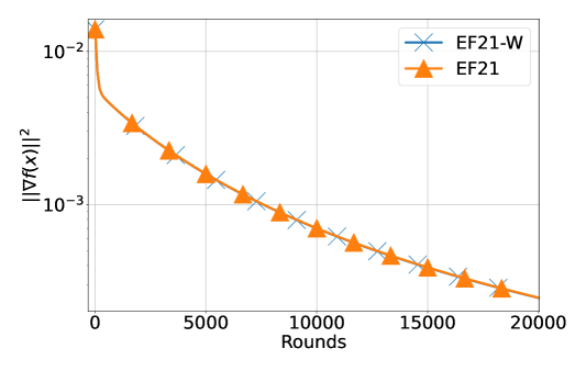
where represents the -th data point out from a set of data points stored at client , and denotes a regularization coefficient. We utilized six datasets from LIBSVM (Chang & Lin, 2011). The dataset shuffling strategy, detailed in Section I.5, was employed to emulate heterogeneous data distribution. Each client was assigned the same number of data points. Figure 1 provides a comparison between EF21 employing the original stepsize (Richtárik et al., 2021) and EF21-W with the better stepsize. The initial gradient estimators were chosen as for all . As evidenced empirically, the EF21-W algorithm emerges as a practical choice when utilized in situations characterized by high variance in smoothness constants. As evident from the plots, the algorithm employing the new step size exhibits superior performance compared to its predecessor.
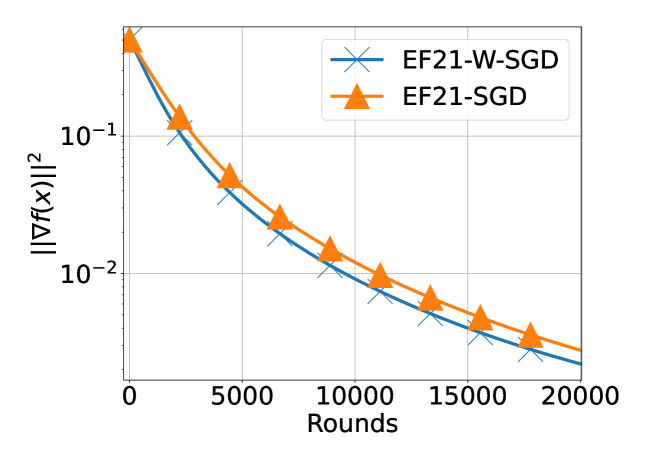
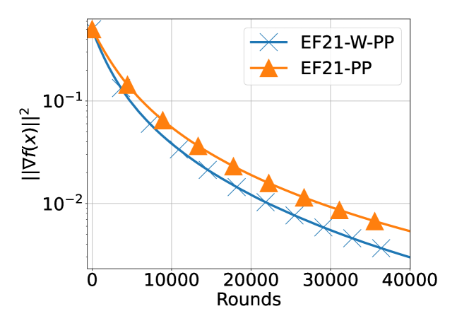
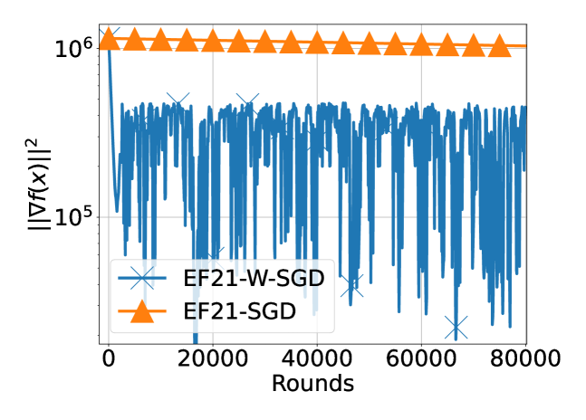
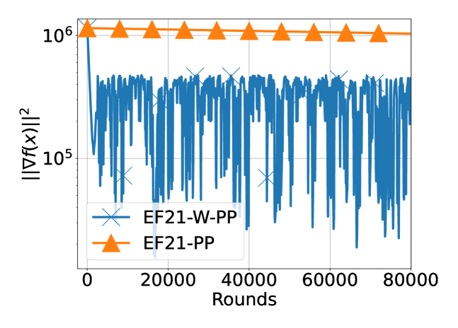
Next, we conducted a comparative analysis of the performance of EF21-W-PP and EF21-W-SGD, as elucidated in the appendix, compared to their non-weighted counterparts. In the EF21-PP/EF21-W-PP algorithms, each client participated independently in each round with probability . Moreover, in the case of EF21-SGD/EF21-W-SGD algorithms, a single data point was stochastically sampled from a uniform distribution at each client during each iteration of the algorithm. As observed in Figure 2, the algorithms employing the new learning rates demonstrate faster convergence. Notably, Figure 2 (c) depicts more pronounced oscillations with updated step sizes, as the new analysis permits larger step sizes, which can induce oscillations in stochastic methods.
3.2 Non-convex linear model on synthetic datasets
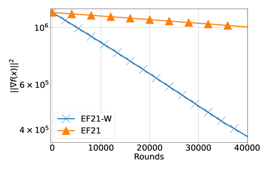
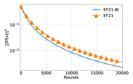
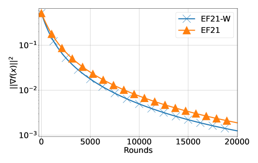
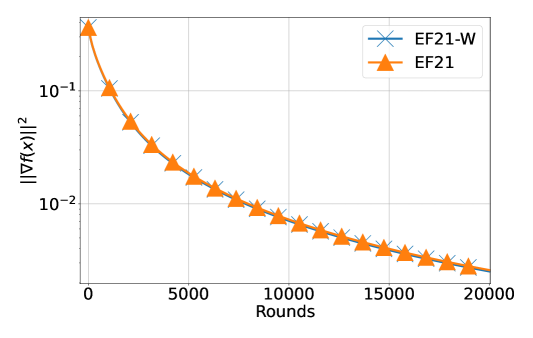
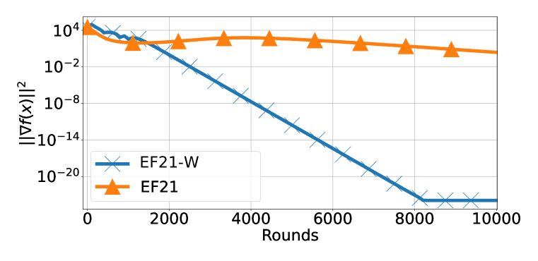
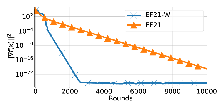
In our second set of experiments, we trained a linear regression model with a non-convex regularizer. The function for the linear regression problem is defined as follows: Here, and represent the feature matrix and labels stored on client encompassing data points. The data employed in four experiments, as illustrated in Figure 3, was generated in such a manner that the smoothness constant remained fixed, while varied so that the difference between two crucial to analysis terms and changed from a relatively large value to negligible. As evident from Figure 3, the performance of EF21-W consistently matches or surpasses that of the original EF21, particularly in scenarios characterized by significant variations in the smoothness constants. For additional details and supplementary experiments, we refer the reader to Sections I and J.



Acknowledgements
This work of all authors was supported by the KAUST Baseline Research Scheme (KAUST BRF). The work Peter Richtárik and Konstantin Burlachenko was also supported by the SDAIA-KAUST Center of Excellence in Data Science and Artificial Intelligence (SDAIA-KAUST AI). We wish to thank Babis Kostopoulos—a VSRP intern at KAUST who spent some time working on this project in Summer 2023—for helping with some parts of the project. We offered Babis co-authorship, but he declined.
References
- Alistarh et al. (2017) Dan Alistarh, Demjan Grubic, Jerry Li, Ryota Tomioka, and Milan Vojnovic. QSGD: Communication-efficient SGD via gradient quantization and encoding. In Advances in Neural Information Processing Systems, 2017.
- Alistarh et al. (2018) Dan Alistarh, Torsten Hoefler, Mikael Johansson, Sarit Khirirat, Nikola Konstantinov, and Cédric Renggli. The convergence of sparsified gradient methods. In Advances in Neural Information Processing Systems, 2018.
- Bernstein et al. (2018) Jeremy Bernstein, Yu-Xiang Wang, Kamyar Azizzadenesheli, and Animashree Anandkumar. signsgd: Compressed optimisation for non-convex problems. In International Conference on Machine Learning, pp. 560–569. PMLR, 2018.
- Bishop (2016) C.M. Bishop. Pattern Recognition and Machine Learning. Information Science and Statistics. Springer New York, 2016. ISBN 9781493938438. URL https://books.google.com.sa/books?id=kOXDtAEACAAJ.
- Burlachenko et al. (2021) Konstantin Burlachenko, Samuel Horváth, and Peter Richtárik. Fl_pytorch: optimization research simulator for federated learning. In Proceedings of the 2nd ACM International Workshop on Distributed Machine Learning, pp. 1–7, 2021.
- Chang & Lin (2011) Chih-Chung Chang and Chih-Jen Lin. LIBSVM: a library for support vector machines. ACM Transactions on Intelligent Systems and Technology (TIST), 2(3):1–27, 2011.
- Condat et al. (2022) Laurent Condat, Kai Yi, and Peter Richtárik. EF-BV: A unified theory of error feedback and variance reduction mechanisms for biased and unbiased compression in distributed optimization. In Advances in Neural Information Processing Systems, volume 35, 2022.
- Condat et al. (2023) Laurent Condat, Grigory Malinovsky, and Peter Richtárik. Tamuna: Accelerated federated learning with local training and partial participation. arXiv preprint arXiv:2302.09832, 2023.
- d’Aspremont et al. (2021) Alexandre d’Aspremont, Damien Scieur, and Adrien Taylor. Acceleration methods. Foundation and Trends in Optimization, 5(1–2):1–245, 2021.
- Dean et al. (2012) Jeffrey Dean, Greg Corrado, Rajat Monga, Kai Chen, Matthieu Devin, Mark Mao, Marc’aurelio Ranzato, Andrew Senior, Paul Tucker, Ke Yang, et al. Large scale distributed deep networks. Advances in Neural Information Processing Systems, 25, 2012.
- Fatkhullin et al. (2021) Ilyas Fatkhullin, Igor Sokolov, Eduard Gorbunov, Zhize Li, and Peter Richtárik. EF21 with bells & whistles: Practical algorithmic extensions of modern error feedback. arXiv preprint arXiv:2110.03294, 2021.
- Fatkhullin et al. (2023) Ilyas Fatkhullin, Alexander Tyurin, and Peter Richtárik. Momentum provably improves error feedback! In Advances in Neural Information Processing Systems, volume 36, 2023.
- Gavriluţ et al. (2009) Dragoş Gavriluţ, Mihai Cimpoeşu, Dan Anton, and Liviu Ciortuz. Malware detection using machine learning. In 2009 International Multiconference on Computer Science and Information Technology, pp. 735–741. IEEE, 2009.
- Gorbunov et al. (2020) Eduard Gorbunov, Filip Hanzely, and Peter Richtárik. A unified theory of SGD: Variance reduction, sampling, quantization and coordinate descent. In The 23rd International Conference on Artificial Intelligence and Statistics, 2020.
- Gorbunov et al. (2021) Eduard Gorbunov, Konstantin Burlachenko, Zhize Li, and Peter Richtárik. MARINA: Faster non-convex distributed learning with compression. In 38th International Conference on Machine Learning, 2021.
- Horváth et al. (2019a) Samuel Horváth, Chen-Yu Ho, Ľudovít Horváth, Atal Narayan Sahu, Marco Canini, and Peter Richtárik. Natural compression for distributed deep learning. arXiv preprint arXiv:1905.10988, 2019a.
- Horváth et al. (2019b) Samuel Horváth, Dmitry Kovalev, Konstantin Mishchenko, Sebastian Stich, and Peter Richtárik. Stochastic distributed learning with gradient quantization and variance reduction. arXiv preprint arXiv:1904.05115, 2019b.
- Horváth et al. (2022) Samuel Horváth, Chen-Yu Ho, Ludovit Horvath, Atal Narayan Sahu, Marco Canini, and Peter Richtárik. Natural compression for distributed deep learning. In Mathematical and Scientific Machine Learning, pp. 129–141. PMLR, 2022.
- IEEE Computer Society (2008) IEEE Computer Society. IEEE Standard for Floating-Point Arithmetic. Technical report, IEEE, 2008. URL {https://ieeexplore.ieee.org/document/4610935}. IEEE Std 754-2008.
- Kairouz et al. (2021) Peter Kairouz, H Brendan McMahan, Brendan Avent, Aurélien Bellet, Mehdi Bennis, Arjun Nitin Bhagoji, Kallista Bonawitz, Zachary Charles, Graham Cormode, Rachel Cummings, et al. Advances and open problems in federated learning. Foundations and Trends® in Machine Learning, 14(1–2):1–210, 2021.
- Khaled & Richtárik (2022) Ahmed Khaled and Peter Richtárik. Better theory for SGD in the nonconvex world. Transactions on Machine Learning Research, 2022.
- Khaled et al. (2023) Ahmed Khaled, Othmane Sebbouh, Nicolas Loizou, Robert M. Gower, and Peter Richtárik. Unified analysis of stochastic gradient methods for composite convex and smooth optimization. Journal of Optimization Theory and Applications, 2023.
- Khirirat et al. (2018) Sarit Khirirat, Hamid Reza Feyzmahdavian, and Mikael Johansson. Distributed learning with compressed gradients. arXiv preprint arXiv:1806.06573, 2018.
- Konečný et al. (2016a) Jakub Konečný, H. Brendan McMahan, Daniel Ramage, and Peter Richtárik. Federated optimization: distributed machine learning for on-device intelligence. arXiv:1610.02527, 2016a.
- Konečný et al. (2016b) Jakub Konečný, H. Brendan McMahan, Felix Yu, Peter Richtárik, Ananda Theertha Suresh, and Dave Bacon. Federated learning: strategies for improving communication efficiency. In NIPS Private Multi-Party Machine Learning Workshop, 2016b.
- Krizhevsky et al. (2012) Alex Krizhevsky, Ilya Sutskever, and Geoffrey E Hinton. Imagenet classification with deep convolutional neural networks. In Advances in Neural Information Processing Systems, volume 25, 2012.
- Li et al. (2020a) Tian Li, Anit Kumar Sahu, Ameet Talwalkar, and Virginia Smith. Federated learning: Challenges, methods, and future directions. IEEE Signal Processing Magazine, 37:50–60, 2020a.
- Li et al. (2019) Xiang Li, Kaixuan Huang, Wenhao Yang, Shusen Wang, and Zhihua Zhang. On the convergence of FedAvg on non-iid data. arXiv preprint arXiv:1907.02189, 2019.
- Li et al. (2020b) Zhize Li, Dmitry Kovalev, Xun Qian, and Peter Richtárik. Acceleration for compressed gradient descent in distributed and federated optimization. In International Conference on Machine Learning, 2020b.
- Li et al. (2021) Zhize Li, Hongyan Bao, Xiangliang Zhang, and Peter Richtárik. PAGE: A simple and optimal probabilistic gradient estimator for nonconvex optimization. In International Conference on Machine Learning (ICML), 2021.
- Lin et al. (2022) Stephanie Lin, Jacob Hilton, and Owain Evans. TruthfulQA: Measuring how models mimic human falsehoods. In Proceedings of the 60th Annual Meeting of the Association for Computational Linguistics (Volume 1: Long Papers), pp. 3214–3252, Dublin, Ireland, May 2022. Association for Computational Linguistics. doi: 10.18653/v1/2022.acl-long.229. URL https://aclanthology.org/2022.acl-long.229.
- Lin et al. (2018) Tao Lin, Sebastian U Stich, Kumar Kshitij Patel, and Martin Jaggi. Don’t use large mini-batches, use local SGD. arXiv preprint arXiv:1808.07217, 2018.
- McMahan et al. (2017) Brendan McMahan, Eider Moore, Daniel Ramage, Seth Hampson, and Blaise Aguera y Arcas. Communication-efficient learning of deep networks from decentralized data. In Artificial intelligence and statistics, pp. 1273–1282. PMLR, 2017.
- Mishchenko et al. (2019) Konstantin Mishchenko, Eduard Gorbunov, Martin Takáč, and Peter Richtárik. Distributed learning with compressed gradient differences. arXiv preprint arXiv:1901.09269, 2019.
- Mishchenko et al. (2022) Konstantin Mishchenko, Grigory Malinovsky, Sebastian Stich, and Peter Richtárik. Proxskip: Yes! Local gradient steps provably lead to communication acceleration! Finally! In International Conference on Machine Learning, pp. 15750–15769. PMLR, 2022.
- Nesterov (1983) Yurii Nesterov. A method for unconstrained convex minimization problem with the rate of convergence o (1/k^ 2), 1983. URL https://cir.nii.ac.jp/crid/1370576118744597902.
- Nesterov (2004) Yurii Nesterov. Introductory lectures on convex optimization: a basic course (Applied Optimization). Kluwer Academic Publishers, 2004.
- Onay & Öztürk (2018) Ceylan Onay and Elif Öztürk. A review of credit scoring research in the age of big data. Journal of Financial Regulation and Compliance, 26(3):382–405, 2018.
- Poplin et al. (2017) Ryan Poplin, Avinash V. Varadarajan, Katy Blumer, Yun Liu, Michael V. McConnell, Gregory S. Corrado, Lily Peng, and Dale R. Webster. Predicting cardiovascular risk factors from retinal fundus photographs using deep learning. arXiv preprint arXiv:1708.09843, 2017.
- Richtárik et al. (2021) Peter Richtárik, Igor Sokolov, and Ilyas Fatkhullin. EF21: A new, simpler, theoretically better, and practically faster error feedback. In Advances in Neural Information Processing Systems, volume 34, 2021.
- Richtárik et al. (2023) Peter Richtárik, Elnur Gasanov, and Konstantin Burlachenko. Error feedback shines when features are rare. arXiv preprint arXiv:2305.15264, 2023.
- Safaryan et al. (2021) Mher Safaryan, Egor Shulgin, and Peter Richtárik. Uncertainty principle for communication compression in distributed and federated learning and the search for an optimal compressor. Information and Inference: A Journal of the IMA, 11(2):557–580, 04 2021. ISSN 2049-8772. doi: 10.1093/imaiai/iaab006. URL https://doi.org/10.1093/imaiai/iaab006.
- Safaryan et al. (2022) Mher Safaryan, Rustem Islamov, Xun Qian, and Peter Richtárik. FedNL: Making Newton-type methods applicable to federated learning. In Internatioanl Conference on Machine Learning, 2022.
- Seide et al. (2014) Frank Seide, Hao Fu, Jasha Droppo, Gang Li, and Dong Yu. 1-bit stochastic gradient descent and its application to data-parallel distributed training of speech DNNs. In Fifteenth Annual Conference of the International Speech Communication Association, 2014.
- Shalev-Shwartz & Ben-David (2014) S. Shalev-Shwartz and S. Ben-David. Understanding Machine Learning: From Theory to Algorithms. Understanding Machine Learning: From Theory to Algorithms. Cambridge University Press, 2014. ISBN 9781107057135. URL https://books.google.com.sa/books?id=ttJkAwAAQBAJ.
- Stich (2018) Sebastian U Stich. Local SGD converges fast and communicates little. arXiv preprint arXiv:1805.09767, 2018.
- Stich et al. (2018) Sebastian U. Stich, J.-B. Cordonnier, and Martin Jaggi. Sparsified SGD with memory. In Advances in Neural Information Processing Systems, 2018.
- Sun et al. (2017) Yu Sun, Yuan Liu, Guan Wang, Haiyan Zhang, et al. Deep learning for plant identification in natural environment. Computational Intelligence and Neuroscience, 2017.
- Szlendak et al. (2022) Rafał Szlendak, Alexander Tyurin, and Peter Richtárik. Permutation compressors for provably faster distributed nonconvex optimization. In International Conference on Learning Representations, 2022.
- Tyurin & Richtárik (2023) Alexander Tyurin and Peter Richtárik. DASHA: Distributed nonconvex optimization with communication compression and optimal oracle complexity. In International Conference on Learning Representations, 2023.
- Vaswani et al. (2017) Ashish Vaswani, Noam Shazeer, Niki Parmar, Jakob Uszkoreit, Llion Jones, Aidan N Gomez, Lukasz Kaiser, and Illia Polosukhin. Attention is all you need. In Advances in Neural Information Processing Systems, volume 30, 2017.
- Verbraeken et al. (2020) Joost Verbraeken, Matthijs Wolting, Jonathan Katzy, Jeroen Kloppenburg, Tim Verbelen, and Jan S Rellermeyer. A survey on distributed machine learning. ACM Computing Surveys, 53(2):1–33, 2020.
- Vogels et al. (2019) Thijs Vogels, Sai Praneeth Karimireddy, and Martin Jaggi. PowerSGD: Practical low-rank gradient compression for distributed optimization. In Advances in Neural Information Processing Systems, 2019.
- Wang et al. (2021) Jianyu Wang, Zachary Charles, Zheng Xu, Gauri Joshi, H. Brendan McMahan, Blaise Aguera y Arcas, Maruan Al-Shedivat, Galen Andrew, Salman Avestimehr, Katharine Daly, Deepesh Data, Suhas Diggavi, Hubert Eichner, Advait Gadhikar, Zachary Garrett, Antonious M. Girgis, Filip Hanzely, Andrew Hard, Chaoyang He, Samuel Horvath, Zhouyuan Huo, Alex Ingerman, Martin Jaggi, Tara Javidi, Peter Kairouz, Satyen Kale, Sai Praneeth Karimireddy, Jakub Konecny, Sanmi Koyejo, Tian Li, Luyang Liu, Mehryar Mohri, Hang Qi, Sashank J. Reddi, Peter Richtarik, Karan Singhal, Virginia Smith, Mahdi Soltanolkotabi, Weikang Song, Ananda Theertha Suresh, Sebastian U. Stich, Ameet Talwalkar, Hongyi Wang, Blake Woodworth, Shanshan Wu, Felix X. Yu, Honglin Yuan, Manzil Zaheer, Mi Zhang, Tong Zhang, Chunxiang Zheng, Chen Zhu, and Wennan Zhu. A field guide to federated optimization. arXiv preprint arXiv:2107.06917, 2021.
- Wang et al. (2023) Jue Wang, Yucheng Lu, Binhang Yuan, Beidi Chen, Percy Liang, Christopher De Sa, Christopher Re, and Ce Zhang. Cocktailsgd: Fine-tuning foundation models over 500mbps networks. In International Conference on Machine Learning, pp. 36058–36076. PMLR, 2023.
- Yang et al. (2019) Tao Yang, Xinlei Yi, Junfeng Wu, Ye Yuan, Di Wu, Ziyang Meng, Yiguang Hong, Hong Wang, Zongli Lin, and Karl H. Johansson. A survey of distributed optimization. Annual Reviews in Control, 47:278–305, 2019. ISSN 1367-5788. doi: https://doi.org/10.1016/j.arcontrol.2019.05.006. URL https://www.sciencedirect.com/science/article/pii/S1367578819300082.
- Zhao & Zhang (2015) Peilin Zhao and Tong Zhang. Stochastic optimization with importance sampling for regularized loss minimization. In Francis Bach and David Blei (eds.), Proceedings of the 32nd International Conference on Machine Learning, volume 37 of Proceedings of Machine Learning Research, pp. 1–9, Lille, France, 07–09 Jul 2015. PMLR. URL https://proceedings.mlr.press/v37/zhaoa15.html.
Appendix A Basic Results and Lemmas
In this section, we offer a few results that serve as essential prerequisites for establishing the main findings in the paper.
A.1 Optimal client cloning frequencies
Lemma 1 (Optimal weights).
Let for . Then
| (17) |
which is achieved when . This means that
| (18) |
We now show that the cloning frequencies given by form a -approximation for the optimization problem of finding the optimal integer client frequencies.
Lemma 2 (-approximation).
If we let for all , then
Proof.
Recall that
The first inequality in the claim follows by relaxing the integrality constraints, which gives us the bound
and subsequently applying Lemma 17.
Next, we argue that the quantity is at most . Indeed,
| (19) |
We will now use this to bound from above:
Since for all , the proof is finished as follows:
∎
A.2 Descent lemma
A.3 Young’s inequality
Lemma 4 (Young’s inequality).
For any and any positive scalar it holds that
| (21) |
A.4 -Suboptimal but simple stepsize rule
Lemma 5 (Lemma 5, Richtárik et al. (2021)).
Let . If then . Moreover, the bound is tight up to the factor of 2 since
A.5 Optimal coefficient in Young’s inequality
Lemma 6 (Lemma 3, Richtárik et al. (2021)).
Let and for , let and . Then, the solution of the optimization problem
| (22) |
is given by . Furthermore, , and .
Appendix B Cloning reformulation for Polyak-Łojaschewitz functions
For completeness, we also provide a series of convergence results under Polyak-Łojasiewicz condition. We commence our exposition with the subsequent definition.
Assumption 4 (Polyak-Łojasiewicz).
There exists a positive scalar such that for all points , the following inequality is satisfied:
| (23) |
where .
Theorem 5.
Appendix C Proof of Theorem 3 (Theory for EF21-W)
In this section, we present a proof for Theorem 3. To start this proof, we establish a corresponding contraction lemma. We define the following quantities:
| (24) |
where the weights are defined as specified in Algorithm 2, that is,
| (25) |
C.1 A lemma
With these definitions in place, we are now prepared to proceed to the lemma.
Lemma 7.
Let for all and . Let . Then, for iterates of Algorithm 2 we have
| (26) |
and
| (27) |
where is an arbitrary positive scalar, and
| (28) |
Proof.
The proof is straightforward and bears resemblance to a similar proof found in a prior work (Richtárik et al., 2021).
with the final inequality holding for any positive scalar . Consequently, we have successfully established the first part of the lemma.
By employing (24) and the preceding inequality, we can derive the subsequent bound for the conditional expectation of :
| (29) | |||||
Applying 2 and (25), we further proceed to:
| (30) | |||||
Using the tower property, we get
and this finalizes the proof. ∎
C.2 Main result
We are now prepared to establish the proof for Theorem 3.
Proof.
Note that, according to (13), the gradient estimate for Algorithm 2 gets the following form:
| (31) |
Using Lemma 3 and Jensen’s inequality applied to the function (since ), we obtain the following bound:
| (32) | |||||
Subtracting from both sides and taking expectation, we get
| (33) |
Let , and Subsequently, by adding (27) with a multiplier, we obtain
The last inequality is a result of the bound which is satisfied for the stepsize
where . Maximizing the stepsize bound over the choice of using Lemma 6, we obtain the final stepsize. By summing up inequalities for we get
Multiplying both sides by , after rearranging we get
It remains to notice that the left hand side can be interpreted as , where is chosen from uniformly at random. ∎
C.3 Main result for Polyak-Łojasiewicz functions
The main result is presented next.
Theorem 6.
Let Assumptions 1, 2, and 4 hold. Assume that for all and . Let the stepsize in Algorithm 2 be set as
Let
Then, for any the following inequality holds:
| (34) |
Proof.
We proceed as in the previous proof, starting from the descent lemma with the same vector but using the PL inequality and subtracting from both sides:
| (35) | |||||
Let , and . Thus,
where and are set as in Lemma 6. Note that our extra assumption on the stepsize implies that and
The last inequality follows from the bound . Thus,
It remains to unroll the recurrence. ∎
Appendix D Proof of Theorem 4 (Improved Theory for EF21)
We commence by redefining gradient distortion as follows:
| (36) |
We recall that the gradient update step for standard EF21 (Algorithm 1) takes the following form:
| (37) | |||
| (38) |
D.1 Two lemmas
Once more, we start our proof with the contraction lemma.
Lemma 8.
Proof.
The proof of this lemma starts as the similar lemma in the standard analysis of EF21:
for all . We proceed the proof as follows:
| (41) | |||||
Note that this is the exact place where the current analysis differs from the standard one. It fully coincides with it when , i.e., when we assign the same weight for each individual gradient distortion . However, applying weights according to “importance” of each function, we proceed as follows:
what finishes the proof. ∎
To prove the main convergence theorem, we also need the following lemma.
Lemma 9.
For the variable from Algorithm 1, the following inequality holds:
| (42) |
Proof.
The proof is straightforward:
where the only inequality in this series of equations is derived using Jensen’s inequality. ∎
D.2 Main result
We are now equipped with all the necessary tools to establish the convergence theorem.
Proof.
Let us define the Lyapunov function
Let us also define . We start as follows:
The inequality in the last but one line is valid if
according to Lemma 5. By optimizing the stepsize bound through the selection of in accordance with Lemma 6, we derive the final stepsize and establish the optimal value for in defining the Lyapunov function. Applying the tower property and unrolling the recurrence, we finish the proof. ∎
D.3 Main result for Polyak-Łojasiewicz functions
For completeness, we also provide a convergence result under Polyak-Łojasiewicz condition (Assumption 4). The main result is presented next.
Theorem 7.
Let Assumptions 1, 2, and 4 hold. Assume that for all and . Let the stepsize in Algorithm 2 be set as
Let
Then, for any the following inequality holds:
| (43) |
Proof.
We proceed as in the previous proof, starting from the descent lemma with the same vector but using the PL inequality and subtracting from both sides:
| (44) | |||||
Let , and . Thus,
Note that our extra assumption on the stepsize implies that and
The last inequality follows from the bound . Thus,
It remains to unroll the recurrence which finishes the prove. ∎
Appendix E EF21-W-SGD: Weighted Error Feedback 2021 with Stochastic Subsampled Gradients
The EF21-W algorithm assumes that all clients can compute the exact gradient in each round. In some scenarios, the exact gradients may be unavailable or too costly to compute, and only approximate gradient estimators can be obtained. In this section, we present the convergence result for EF21-W in the setting where the gradient computation on the clients, , is replaced by a specific stochastic gradient estimator. For a variation of EF21-W-SGD which is working under a more general setting please see Appendix F.
E.1 Algorithm
In this section, we extend EF21-W to handle stochastic gradients, and we call the resulting algorithm EF21-W-SGD (Algorithm 3). Our analysis of this extension follows a similar approach as the one used by Fatkhullin et al. (2021) for studying the stochastic gradient version of the vanilla EF21 algorithm, which they called EF21-SGD. Analysis of EF21-W-SGD has two important differences with vanilla EF21-SGD:
-
1.
Vanilla EF21-SGD provides maximum theoretically possible , where EF21-W-SGD has
- 2.
Assumption 5 (General assumption for stochastic gradient estimators).
We assume that for all there exist parameters , such that
| (45) |
holds for all , where333When one can ignore the first term in the right-hand side of (45), i.e., assumption is not required in this case. .
We study EF21-W-SGD under the same assumption as was used for analyzing Vanilla EF21-SGD, which we denote as Assumption 5. To the best of our knowledge, this assumption, which was originally presented as Assumption 2 by Khaled & Richtárik (2022), is the most general assumption for a stochastic gradient estimator in a non-convex setting.
Next, to be aligned with original Vanilla EF21-SGD (Fatkhullin et al., 2021) we have considered a specific form of gradient estimator. This specific form of gradient estimator from Vanilla EF21-SGD presented in Section 4.1.2. of Fatkhullin et al. (2021) where the stochastic gradient has been computed as follows:
Here is a minibatch size of sampled datapoint indexed by of client in iteration . And are independent random variables. For a version of EF21-W-SGD which is working under a more general setting please see Appendix F.
E.2 A lemma
The contraction lemma in this case gets the following form:
Proof.
Define . The proof starts as follows:
To further bound the last term, which contains multiple factors, we leverage the property that is a random variable serving as an unbiased estimator of , taking the form
where are independent random variables. Next, we can continue as follows:
Furthermore, as a result of leveraging 2, we can derive the subsequent bound:
Applying the tower property and subsequently taking the expectation, we obtain:
| (47) | ||||
Regarding the expectation of , we derive the subsequent bound:
Employing quantities and , the final bound can be reformulated as follows:
Given that , we have:
what completes the proof. ∎
E.3 Main result
Now we are ready to prove the main convergence theorem.
Theorem 8.
Let for all and in Algorithm 3. Set the following quantities:
Under Assumptions 1, 2, and 5, and selection of , such that set the stepsize in the following way:
| (48) |
Choose an iterate from with probability
| (49) |
where
Then,
| (50) |
where .
Proof.
Subtracting from both sides and taking expectation, we get
| (53) | |||||
Let , and Then by adding and employing (46), we obtain:
The last inequality follows from the bound , which holds due to Lemma 5 for Subsequently, we will reconfigure the final inequality and perform algebraic manipulations, taking into account that . In the final step of these algebraic transformations, we will leverage the fact that :
Therefore,
Further,
We sum up inequalities above with weights , where and :
Finally, we notice that , what concludes the proof. ∎
Appendix F EF21-W-SGD: Weighted Error Feedback 2021 with Stochastic Gradients under the ABC Assumption
In this section, we present the convergence result for Weighted EF21 in the setting where the gradient computation on the clients is replaced with a pretty general unbiased stochastic gradient estimator.
F.1 Algorithm
The EF21-W algorithm assumes that all clients can compute the exact gradient in each round. In some scenarios, the exact gradients may be unavailable or too costly to compute, and only approximate gradient estimators can be obtained. To have the ability for EF21-W to work in such circumstances we extended EF21-W to handle stochastic gradients. We called the resulting algorithm EF21-W-SGD (Algorithm 4).
Our analysis of this extension follows a similar approach as the one used by Fatkhullin et al. (2021) for studying the stochastic gradient version under the name EF21-SGD. However, EF21-W-SGD has four important differences with vanilla EF21-SGD:
- 1.
-
2.
Vanilla EF21-SGD provides maximum theoretically possible , where EF21-W-SGD has .
-
3.
In contrast to the original analysis Vanilla EF21-SGD our analysis provides a more aggressive parameter which is smaller by a factor of .
- 4.
Assumption 6 (General assumption for stochastic gradient estimators).
We assume that for all there exist parameters , such that
| (54) |
holds for all , where444When one can ignore the first term in the right-hand side of (54), i.e., assumption is not required in this case. .
Assumption 7 (Unbiased assumption for stochastic gradient estimators).
We assume that for all there following holds for all :
We study EF21-W-SGD under Assumption 6 and Assumption 7.To the best of our knowledge, this Assumption 6, which was originally presented as Assumption 2 by Khaled & Richtárik (2022), is the most general assumption for a stochastic gradient estimator in a non-convex setting. For a detailed explanation of the generality of this assumption see Figure 1 of Khaled & Richtárik (2022).
F.2 A lemma
The contraction lemma in this case gets the following form:
Lemma 11.
Proof.
Define . The proof starts as follows:
Further, we continue as follows
To further bound the last term, which contains multiple factors, we leverage the property that is a random variable serving as an unbiased estimator of . Our approach is as follows:
Now due to the requirement of unbiasedness of gradient estimators expressed in the form of Assumption 7 we have the following:
| (56) |
Using this variance decomposition, we can proceed as follows.
Next leveraging 2 we replace the second term in the last expression, and we can derive the subsequent bound:
Applying the tower property and subsequently taking the expectation, we obtain:
| (57) | ||||
Next for the expectation of the main quantity of our interest , we derive the subsequent bound:
Employing quantities and , the final bound can be reformulated as follows:
Given that , we have:
what completes the proof. ∎
F.3 Main result
Now we are ready to prove the main convergence theorem.
Theorem 9.
Let for all and in Algorithm 4. set the following quantities:
Under Assumptions 1, 2, 6, 7, and selection of small enough such that holds, set the stepsize in the following way:
| (58) |
Choose an iterate from with probability
| (59) |
where
Then,
| (60) |
where .
Proof.
Subtracting from both sides and taking expectation, we get
Let , and Then by adding and employing inequality (46), we obtain:
The last inequality follows from the bound , which holds due to Lemma 5 for
Subsequently, we will reconfigure the final inequality and perform algebraic manipulations, taking into account that . In the final step of these algebraic transformations, we will leverage the fact that :
Therefore,
Further,
We sum up inequalities above with weights , where and :
Finally, we notice that , what concludes the proof. ∎
Appendix G EF21-W-PP: Weighted Error Feedback 2021 with Partial Participation
In this section, we present another extension of error feedback. Again, to maintain brevity, we show our results for EF21-W, however, we believe getting an enhanced rate for standard EF21 should be straightforward.
G.1 Algorithm
Building upon the delineation of EF21-W in Algorithm 2, we turn our attention to its partial participation variant, EF21-W-PP, and seek to highlight the primary distinctions between them. One salient difference is the introduction of a distribution, denoted as , across the clients. For clarity, consider the power set of the set , representing all possible subsets of . Then, the distribution serves as a discrete distribution over .
While EF21-W-PP runs, at the start of each communication round , the master, having computed a descent step as , samples a client subset from the distribution . Contrasting with Algorithm 2 where the new iteration is sent to all clients, in this variant, it is sent exclusively to those in .
Any client adheres to procedures akin to EF21-W: it compresses the quantity and transmits this to the master. Conversely, client omitted in , i.e., , is excluded from the training for that iteration. Concluding the round, the master updates by integrating the averaged compressed variances received from clients in the set .
Assume is drawn from the distribution . Let us denote
| (62) |
In other words, represents the probability of client being selected in any iteration. For given parameters such that for , we introduce the notations and , respectively.
G.2 A lemma
Having established the necessary definitions, we can now proceed to formulate the lemma.
Lemma 12.
Let for all and . Let 2 hold. Define
| (63) |
For any and , let us define the following quantities:
Additionally, assume that
Then, we have
| (64) |
Proof.
Let us define . If client participates in the training at iteration , then
Utilizing the tower property and taking the expectation with respect to , we derive:
| (65) |
where , and . We now aim to bound the quantity , starting with an application of the tower property:
We combine the two preceding bounds:
Consequently, for , we derive the subsequent bound:
where we applied the preceding inequality. Remembering the definitions and , we subsequently obtain:
Applying (63) and (25), we obtain:
Subsequently, in order to simplify the last inequality, we introduce the variables and :
Therefore,
Expressed in terms of these variables, the final inequality can be reformulated as:
Since we need the contraction property over the gradient distortion , we require . We rewrite these conditions as follows:
∎
G.3 Main result
We are ready to prove the main convergence theorem.
Theorem 10.
Consider Algorithm 5 (EF21-W-PP) applied to the distributed optimization problem (1). Let Assumptions 1, 2, 3 hold, assume that for all and , set
where for all , and let the stepsize satisfy
| (67) |
where , , and
Additionally, assume that
If for we define as an element of the set chosen uniformly at random, then
| (68) |
Proof.
Following the same approach employed in the proof for the SGD case, we obtain
Let , and Applying the previous lemma, we obtain:
By summing up inequalities for we get
Finally, via multiplying both sides by , after rearranging we get:
It remains to notice that the left-hand side can be interpreted as , where is chosen from the set uniformly at random. ∎
Our analysis of this extension follows a similar approach as the one used by Fatkhullin et al. (2021), for algorithm they called EF21-PP. Presented analysis of EF21-W-PP has a better provides a better multiplicative factor in definition of , where in vanilla EF21-PP had . This fact improves upper bound on allowable step size in (67).
Appendix H Improved Theory for EF21 in the Rare Features Regime
In this section, we adapt our new results to the rare features regime proposed and studied by Richtárik et al. (2023).
H.1 Algorithm
In this section, we focus on Algorithm 6, which is an adaptation of EF21 (as delineated in Algorithm 1) that specifically employs Top operators. This variant is tailored for the rare features scenario, enhancing the convergence rate by shifting from the average of squared Lipschitz constants to the square of their average. The modifications introduced in Algorithm 6, compared to the standard EF21, are twofold and significant.
Primarily, the algorithm exclusively engages Top compressors, leveraging the inherent sparsity present in the data. Additionally, the initial gradient estimates are confined to the respective subspaces , as characterized by equation (71). With the exception of these distinct aspects, the algorithm’s execution parallels that of the original EF21.
H.2 New sparsity measure
To extend our results to the rare features regime, we need to slightly change the definition of the parameter in the original paper. The way we do it is unrolled as follows. First, we recall the following definitions from (Richtárik et al., 2023):
| (69) |
and
| (70) |
We also need the following definition of :
| (71) |
H.3 Lemmas
We will proceed through several lemmas.
Lemma 13.
Let for all . Then, the following inequality holds:
| (73) |
Proof.
Initially, we observe that
| (74) |
We note that for any it holds that
| (75) | ||||
where on the last line we used the Jensen’s inequality. Subsequent arithmetic manipulations and the incorporation of definition (72) yield:
| (76) | |||||
Lemma 14.
Assume that for all . Then, it holds for all that
| (77) |
Proof.
For the convenience of the reader, we briefly revisit Lemma 6 from (Richtárik et al., 2023).
Now, we proceed to the following lemma, which aims to provide a tighter bound for the quantity .
Lemma 16.
If 2 holds, then
| (80) |
Proof.
The proof commences as follows:
| (81) | |||||
To advance our derivations, we consider the maximum value over :
what completes the proof. ∎
For clarity and easy reference, we recapitulate Lemma 10 from Richtárik et al. (2023).
Lemma 17 (Lemma 10 from Richtárik et al. (2023)).
Lemma 18.
Under 2, iterates of Algorithm 6 satisfies
| (83) |
H.4 Main result
And now we are ready to formulate the main result.
Theorem 11.
Let Assumptions 1, 2 and 3 hold. Let for all ,
Under these conditions, the iterates of Algorithm 6 satisfy
| (84) |
Proof.
Let us define the Lyapunov function:
| (85) |
We start the proof as follows:
Unrolling the inequality above, we get
from what the main result follows. ∎
Appendix I Experiments: Further Details
I.1 Computing and software environment
We used the Python software suite FL_PyTorch (Burlachenko et al., 2021) to simulate the distributed environment for training. We carried out experiments on a compute node with Ubuntu 18.04 LTS, GBytes of DRAM DDR4 memory at GHz, and cores ( sockets with cores per socket) of Intel(R) Xeon(R) Gold 6246 CPU at GHz. We used double-precision arithmetic during computing gradient oracles. All our computations were carried on CPU.
I.2 Comments on the improvement
The standard EF21 analysis (Richtárik et al., 2021) allows to utilize EF21 with maximum allowable step size equal to:
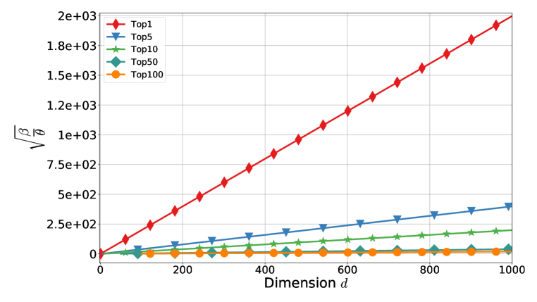
Our analysis allows us to replace the quantity with . This improvement has an important consequence. The replaced quantity affects the step size by a factor of . This factor can be arbitrarily large as increases, as shown in Figure 4. If is increasing and the parameter of TopK compressor is fixed, then even a small improvement in the constant term can have a significant impact in an absolute sense to the computed step size if .
I.3 When improved analysis leads to more aggressive steps
The quantity plays essential role in EF21 analysis. As we saw with special consideration this quantity for EF21 and its extensions is improvable. The improved analysis allows us to replace it with Clearly, by the arithmetic-quadratic mean inequality,
The difference can be expressed as follows:
The coefficient in the last equation can be bounded from below and above as follows:
As a consequence, difference is bound above by the estimated variance of divided by the mean of , also known as Index of Dispersion in statistics. From this consideration, we can more easily observe that EF21-W can have an arbitrarily better stepsize than vanilla EF21 if the variance of is increasing faster than the mean of .
I.4 Dataset generation for synthetic experiment
First, we assume that the user provides two parameters: and . These parameters define the construction of strongly convex function , which are modified by meta-parameters and , described next.
-
1.
Each client initially has
where is initialized in such way that is smooth and strongly convex. Parameters are defined in the following way:
-
2.
The scalar value informally plays the role of meta parameter to change the distribution of and make values of close to one of the following: (i) ; (ii) ; (iii) . The exact modification of depends on the sign of meta parameter .
-
•
Case . In this case for first (i.e., ) compute the value , where is standard linear interpolation
The last () compute the value . For example, if then , and if then for first clients and for last clients.
-
•
Case . In this for all clients the new value . In this case for example if then and if then .
The process firstly fills the in such form that forms a uniform spectrum in with the center of this spectrum equal to . And then as , the variance of is increasing.
-
•
-
3.
We use these new values for all clients as a final target values. Due to numerical issues, we found that it’s worthwhile for the first and last client to add extra scaling. First client scales by factor , and last -th client scales by factor . Here is an additional meta-parameter.
-
4.
Next obtained values are used to generate in such way that has uniform spectrum in .
-
5.
As a last step the objective function is scaled in such a way that it is smooth with constant value . The for each client is initialized as , where is fixed solution.
I.5 Dataset shuffling strategy for LIBSVM dataset
Our dataset shuffling strategy heuristically splits data points so that is maximized. It consists of the following steps:
-
1.
Sort data points from the whole dataset according to constants. Sort all data points according to the smoothness constants of the loss function for each single data point.
-
2.
Assign a single data point to each client Assume that there are total data points in the datasets, and the total number of clients is . At the beginning each client holds a single data point .
-
3.
Pass through all points. Initialize set . Next, we pass through all points except those assigned from the previous step. For each point we find the best client to assign the point in a way that assignment of point to client maximize . Once the client already has data points assigned to it, the client is added to the set .
The set in the last step guarantees each client will have data points. In general, this is a heuristic greedy strategy that approximately maximizes under the constraint that each client has the same amount of data points equal to . Due to its heuristic nature, the Algorithm does not provide deep guarantees, but it was good enough for our experiments.
Appendix J Additional Experiments
In this section, we present additional experiments for comparison EF21-W, EF21-W-PP, EF21-W-SGD with their vanilla versions. We applied these algorithms in a series of synthetically generated convex and non-convex optimization problems and for training logistic regression with non-convex regularized with using several LIBSVM datasets (Chang & Lin, 2011). While carrying out additional experiments we will use three quantities. These quantities have already been mentioned in the main part, but we will repeat them here:
The relationship between these quantities was discussed in Appendix I.3. In our experiments we used TopK compressor. The TopK compressor returns sparse vectors filled with zeros, except positions, which correspond to maximum values in absolute value and which are unchanged by the compressor. Even if this compressor breaks ties arbitrarily, it is possible to show that . The compressor parameter is defined without considering properties of . The quantities , , are derived from , and they do not depend on .
J.1 Additional experiments for EF21
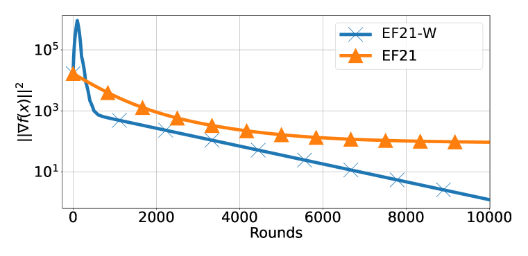
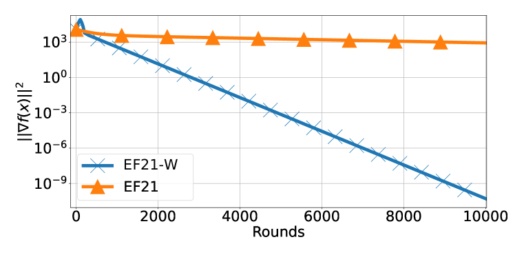
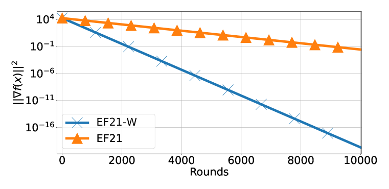
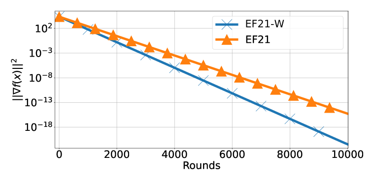
Convex case with synthetic datasets.
We aim to solve optimization problem (1) in the case when the functions are strongly convex. In particular, we work with
| (86) |
where . It can be shown that . The result of experiments for training linear regression model with a convex regularized is presented in Figure 5. The total number of rounds for simulation is . Instances of optimization problems were generated for values , with several values of with using the dataset generation schema described in Appendix I.4. The summary of derived quantities is presented in Table 1. We present several optimization problems to demonstrate the possible different relationships between and . As we see from experiments, the EF21-W is superior as the variance of tends to increase. The plots in Figure 5 (a)–(d) correspond to decreasing variance of . As we see, as the variance of decreases, the difference between EF21-W and EF21 also tends to decrease. Finally, EF21-W is always at least as best as EF21.
| Tag | |||||||||
|---|---|---|---|---|---|---|---|---|---|
| (a) | |||||||||
| (b) | |||||||||
| (c) | |||||||||
| (d) |
Non-convex case with synthetic datasets.
We aim to solve optimization problem (1) in the case when the functions are non-convex. In particular, we work with
| (87) |


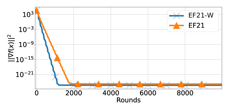
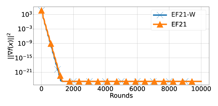
The result of experiments for training linear regression model with a non-convex regularization is presented in Figure 6. The regularization coefficient . Instances of optimization problems were generated for values and several values of for employed dataset generation schema from Appendix I.4.
The summary of derived quantities is presented in Table 2. We present various instances of optimization problems to demonstrate the different relationships between and . As we see in the case of small variance of algorithm EF21-W is at least as best as standard EF21.
| Tag | |||||||||
|---|---|---|---|---|---|---|---|---|---|
| (a) | |||||||||
| (b) | |||||||||
| (c) | |||||||||
| (d) |
Non-convex logistic regression on benchmark datasets.
We aim to solve optimization problem (1) in the case when the functions are non-convex. In particular, we work with logistic regression with a non-convex robustifying regularization term:
| (88) |
where .
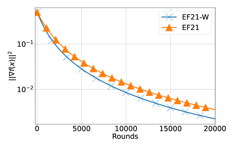
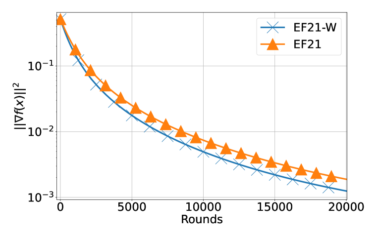
We used several LIBSVM datasets (Chang & Lin, 2011) for our benchmarking purposes. The results are presented in Figure 7 and Figure 8. The important quantities for these instances of optimization problems are summarized in Table 3. From Figures 7 (a), (b), (c), we can observe that for these datasets, the EF21-W is better, and this effect is observable in practice. For example, from these examples, we can observe that K rounds of EF21-W corresponds to only K rounds of EF21. This improvement is essential for Federated Learning, in which both communication rounds and communicate information during a round represent the main bottlenecks and are the subject of optimization. Figures 7 (d), (e), (f) demonstrate that sometimes the EF21-W can have practical behavior close to EF21, even if there is an improvement in step-size (For exact values of step size see Table 3). The experiment on AUSTRALIAN datasets are presented in Figure 8. This example demonstrates that in this LIBSVM benchmark datasets, the relative improvement in the number of rounds for EF21-W compared to EF21 is considerable. For example K rounds of EF21 corresponds to K rounds of EF21-W in terms of attainable .
| Tag | |||||||
|---|---|---|---|---|---|---|---|
| (a) W1A | |||||||
| (b) W2A | |||||||
| (c) W3A | |||||||
| (d) MUSHROOMS | |||||||
| (e) SPLICE | |||||||
| (f) PHISHING | |||||||
| (g) AUSTRALIAN |

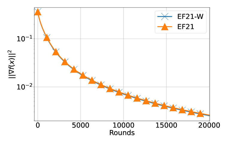
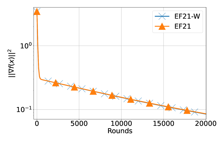
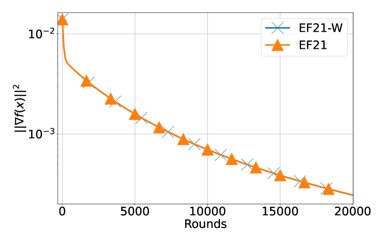
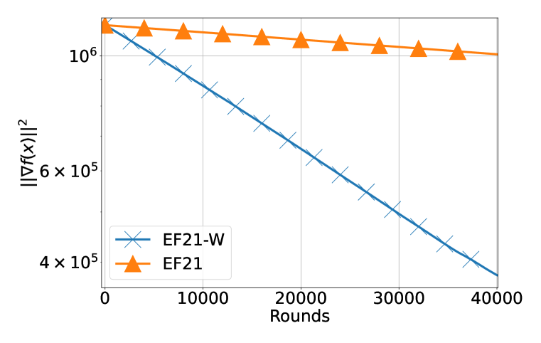
Non-convex logistic regression with non-homogeneous compressor.
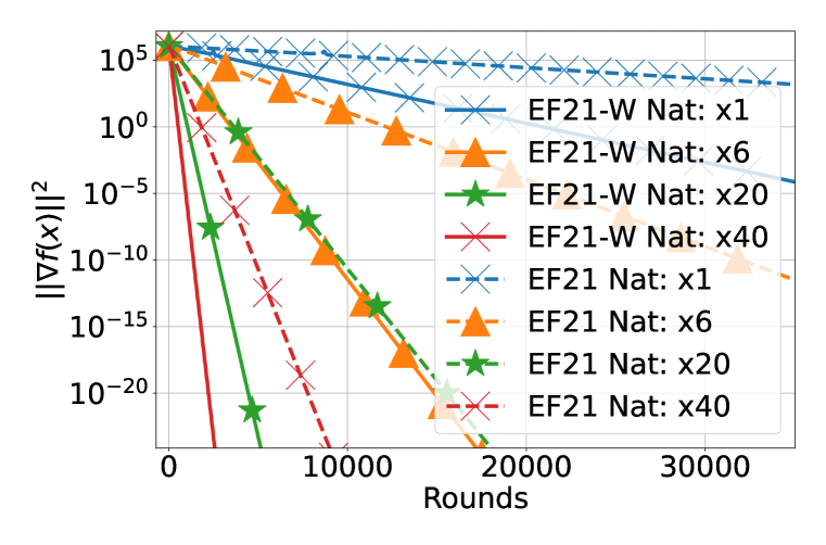
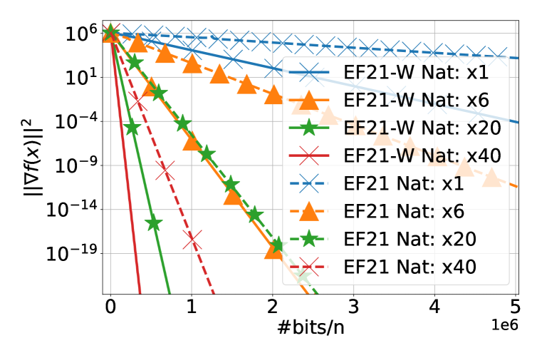
In this supplementary experiment, we leveraged the AUSTRALIAN LIBSVM datasets (Chang & Lin, 2011) to train logistic regression, incorporating a non-convex sparsity-enhanced regularization term defined in Eq. (88). The experiment featured the utilization of a non-homogeneous compressor known as Natural by Horváth et al. (2022), belonging to the family of unbiased compressors and adhering to Definition 3 with . This compressor, in a randomized manner, rounds the exponential part and zeros out the transferred mantissa part when employing the standard IEEE 754 Standard for Floating-Point Arithmetic IEEE Computer Society (2008) representation for floating-point numbers. Consequently, when using a single float-point format (FP32) during communication, only bits of payload per scalar need to be sent to the master, and the remaining bits of mantissa can be entirely dropped.
The experiment results are depicted in Figure 9. In this experiment, we fine-tuned the theoretical step size by multiplying it with a specific constant. As we can see the EF21-W consistently outperforms EF21 across all corresponding step-size multipliers. As we see EF21-W operates effectively by utilizing unbiased non-homogeneous compressors, and the advantages over EF21 extend beyond the scope of applying EF21-W solely to homogeneous compressors. Finally, it is worth noting that the increased theoretical step size in EF21-W does not entirely capture the practical scenario of potentially enhancing the step size by a significantly large multiplicative factor (e.g., ), which remains a subject for future research.
J.2 Additional experiments for EF21-W-PP
Convex case with synthetic datasets.
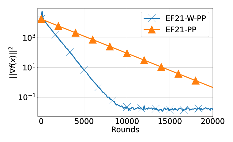
| Tag | |||||||||
|---|---|---|---|---|---|---|---|---|---|
| (a) | |||||||||
| (b) | |||||||||
| (c) |
We aim to solve optimization problem (1) in the case when the functions are strongly convex. In particular, we choose:
| (89) |
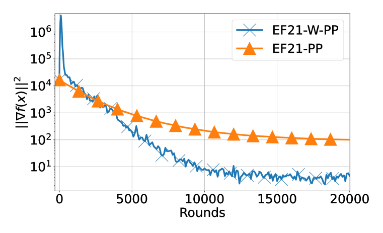
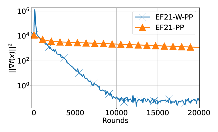
In this synthetic experiment, we have used the maximum allowable step size suggested by the theory of EF21-PP and for the proposed EF21-W-PP algorithm. The initial gradient estimators have been initialized as for all . The number of clients in simulation , dimension of optimization problem , number of samples per client , and number of communication rounds is . For both EF21-PP and EF21-W-PP clients we used Top1 biased contractile compressor. In our experiment, each client’s participation in each communication round is governed by an independent Bernoulli trial which takes . The result of experiments for training linear regression model with a convex regularizer is presented in Figure 10. The regularization constant was chosen to be . Instances of optimization problems were generated for values , with several values of and . The summary of derived quantities is presented in Table 4. We present several optimization problems to demonstrate the possible different relationships between and . As we see from experiments, the EF21-W-PP is superior as the variance of tends to increase. As we can observe EF21-W-PP is always at least as best as EF21-PP.
Non-convex logistic regression on benchmark datasets.
We provide additional numerical experiments in which we compare EF21-PP and EF21-W-PP for solving (1). We address the problem of training a binary classifier via a logistic model on several LIBSVM datasets (Chang & Lin, 2011) with non-convex regularization. We consider the case when the functions are non-convex; in particular, we set as follows:
| (90) |
where .
We conducted distributed training of a logistic regression model on W1A, W2A, W3A, PHISHING, and AUSTRALIAN datasets with non-convex regularization. The initial gradient estimators are set for all . For comparison of EF21-PP and EF21-W-PP, we used the largest step size allowed by theory. We used the dataset shuffling strategy described in Appendix I.5. The results are presented in Figure 11 and Figure 12. The important quantities for these instances of optimization problems are summarized in Table 5.
| Tag | ||||||
|---|---|---|---|---|---|---|
| (a) W1A | ||||||
| (b) W2A | ||||||
| (c) W3A | ||||||
| (d) PHISHING | ||||||
| (e) AUSTRALIAN |
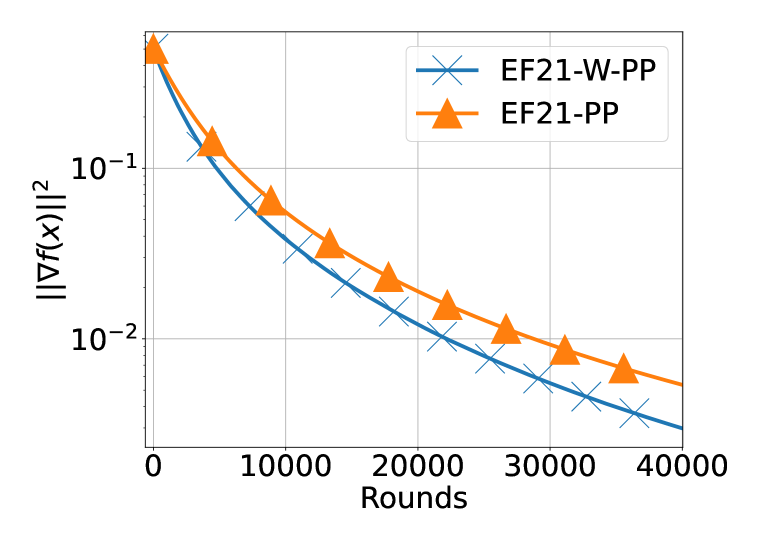
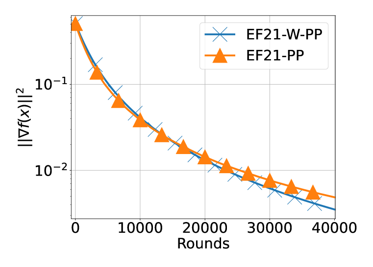
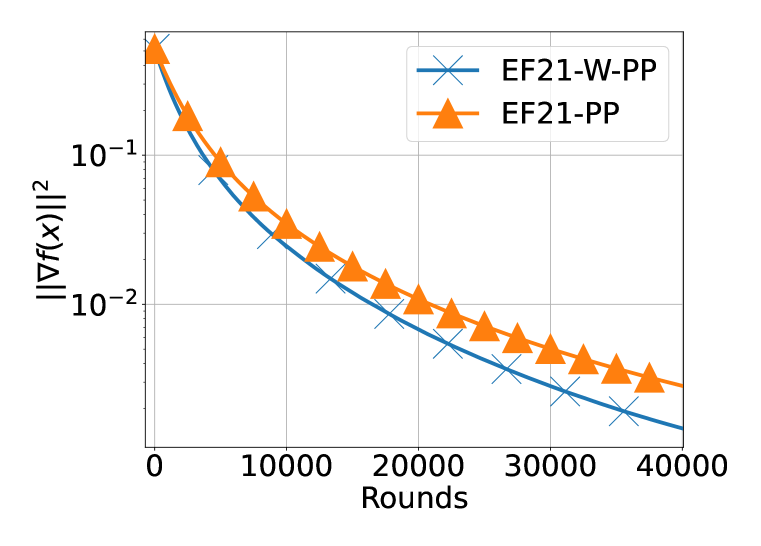
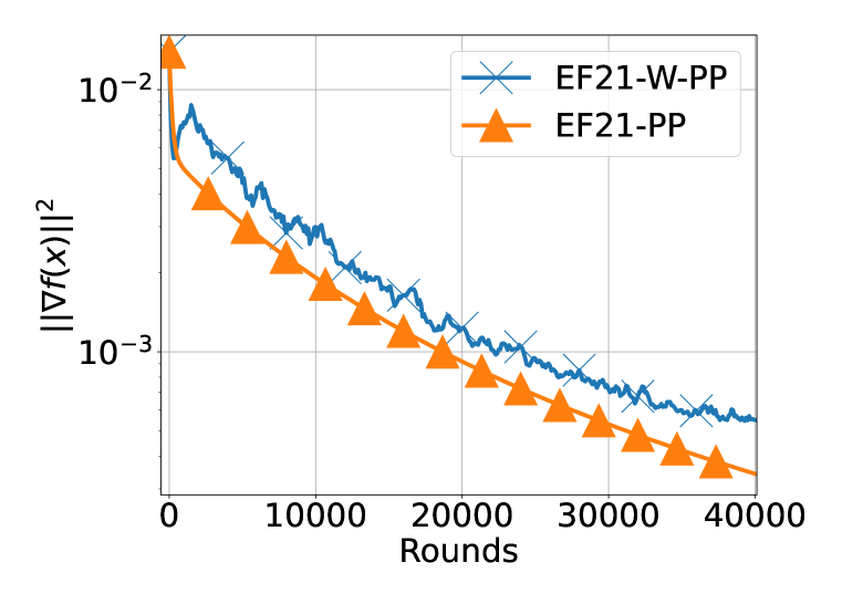
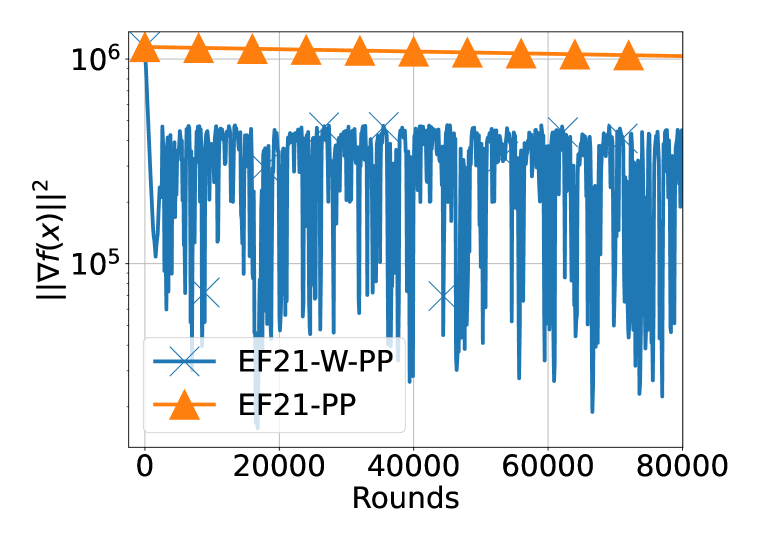
From Figure 11 (a), (b), (c), we can observe that for these datasets, the EF21-W-PP is better, and this effect is observable in practice and is not negligible. Figures 11 (d), demonstrate that sometimes EF21-W-PP in terms of the full gradient at last iterate can have slightly worse behavior compared to EF21-PP, even though theory allow more aggressive step-size (For exact values of step size see Table 5. The experiment on AUSTRALIAN dataset is presented in Figure 12. This example demonstrates that in this LIBSVM benchmark datasets, the relative improvement in the number of rounds for EF21-W-PP compared to EF21-PP is considerable. The EF21-W-PP exhibits more oscillation behavior in terms of for AUSTRALIAN dataset, however as we can see observe in expectation tends to decrease faster compare to EF21-PP.
J.3 Additional experiments for EF21-W-SGD
The standard EF21-SGD with the analysis described in Corollary 4 (Fatkhullin et al., 2021) allows performing the optimization procedure with maximum allowable step size up to the factor of equal to:
In last expression quantities , and . Improved analysis for EF21-W-SGD allows to apply step size:
Therefore in terms of step size
and EF21-W-SGD exhibits a more aggressive step-size.
We conducted distributed training of a logistic regression model on W1A, W2A, W3A, PHISHING, AUSTRALIAN datasets with non-convex regularization. For all datasets, we consider the optimization problem (1), where
| (91) |
and .
The initial gradient estimators are set to for all . For comparison of EF21-SGD and EF21-W-SGD, we used the largest step size allowed by theory. The dataset shuffling strategy repeats the strategy that we have used for EF21-W-PP and EF21-W and it is described in Appendix I.5. The algorithms EF21-SGD and /EF21-W-SGD employed an unbiased gradient estimator, which was estimated by sampling a single training point uniformly at random and independently at each client.
| Tag | ||||||
|---|---|---|---|---|---|---|
| (a) W1A | ||||||
| (b) W2A | ||||||
| (c) W3A | ||||||
| (f) PHISHING | ||||||
| (g) AUSTRALIAN |
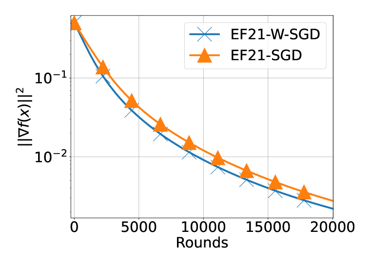
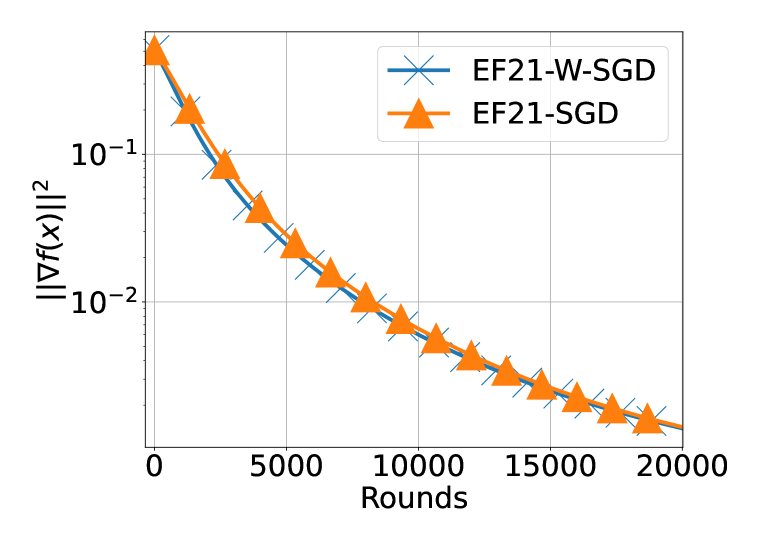
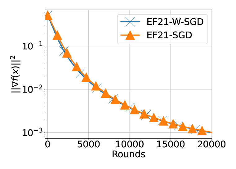
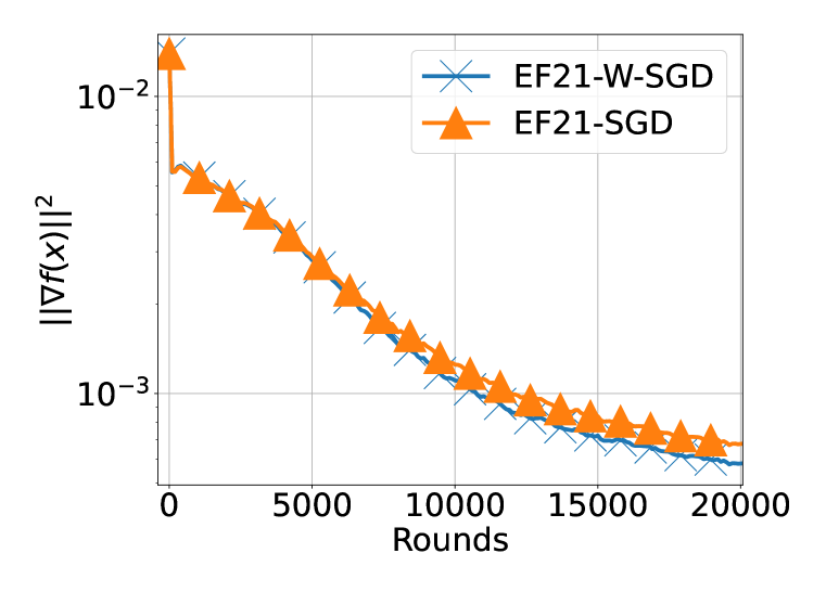
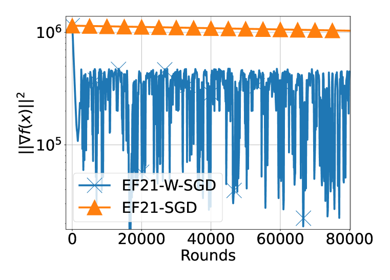
The results are presented in Figure 13 and Figure 14. The important quantities for these instances of optimization problems are summarized in Table 6. In all Figures 13 (a), (b), (c), (d) we can observe that for these datasets, the EF21-W-SGD is better, and this effect is observable in practice. The experiment on AUSTRALIAN datasets are presented in Figure 14. This example demonstrates that in this LIBSVM benchmark datasets, the relative improvement in the number of rounds for EF21-W-SGD compared to EF21-SGD is considerable. Finally, we address oscillation behavior to the fact that employed step size for EF21-SGD is too pessimistic, and its employed step size removes oscillation of .
Appendix K Reproducibility Statement
To ensure reproducibility, we use the following FL_PyTorch simulator features: (i) random seeds were fixed for data synthesis; (ii) random seeds were fixed for the runtime pseudo-random generators involved in EF21-PP and EF21-SGD across clients and the server; (iii) the thread pool size was turned off to avoid the non-deterministic order of client updates in the server.
If you are interested in the source code for all experiments, please contact the authors.