Optimal Savings and Value of Population in A Stochastic Environment: Transient Behavior

We dedicate this paper to the memory of Kenneth J. Arrow; it extends the research he initiated and pursued further with a coauthor of this paper.

Abstract

We extend the work on optimal investment and consumption of a population considered in [2] to a general stochastic setting over a finite time horizon. We incorporate the Cobb-Douglas production function in the capital dynamics while the consumption utility function and the drift rate in the population dynamics can be general, in contrast with [2, 30, 31]. The dynamic programming formulation yields an unconventional nonlinear Hamilton-Jacobi-Bellman (HJB) equation, in which the Cobb-Douglas production function as the coefficient of the gradient of the value function induces the mismatching of power rates between capital and population. Moreover, the equation has a very singular term, essentially a very negative power of the partial derivative of the value function with respect to the capital, coming from the optimization of control, and their resolution turns out to be a complex problem not amenable to classical analysis. To show that this singular term, which has not been studied in any physical systems yet, does not actually blow up, we establish new pointwise generalized power laws for the partial derivative of the value function. Our contribution lies in providing a theoretical treatment that combines both the probabilistic approach and theory of partial differential equations to derive the pointwise upper and lower bounds as well as energy estimates in weighted Sobolev spaces. By then, we accomplish showing the well-posedness of classical solutions to a non-canonical parabolic equation arising from a long-lasting problem in macroeconomics.

Unlike the stationary problem in [2], the intricate transient behavior is only evident over finite time horizons; particularly, if the production function $F$ is dominant, the capital will be steadily built and then reach an equilibrium level; otherwise, with a weak influence of $F$, the capital will gradually shrink to a lower level. Further, due to the nonlinearity of the system, there could be a phase transition at certain critical parameter thresholds, under which an overshooting (undershooting, resp.) of the capital dynamics can be observed when the initial population is larger (smaller, resp.) than the equilibrium level. However, the presence of large enough volatility in the capital investment detours us from determining what the exact transient mechanism of the underlying economy is.

Keywords: Cobb-Douglas production function; Stochastic logistic growth model for population; Stochastic optimal control; Two-dimensional Hamilton-Jacobi-Bellman equation; Weighted Sobolev theory; Control of growth rate; Schauder’s fixed point theorem.

1. Introduction

1.1. Literature review

In 1928, Frank Ramsey [32] introduced the dynamic problem of optimal savings. He used the calculus of variations to derive the general principle of maximizing society’s enjoyment by equating the product of the savings rate and the marginal utility of consumption with the bliss point (the maximum obtainable enjoyment rate minus the actual total utility rate). Ever since, economists and financial mathematicians have extensively explored various versions of the optimal savings problem; for instances, various related works can be founded in [4, 6, 8, 9, 13, 15, 19, 21, 22, 26, 28, 33, 35, 36].

Following Arrow et al. [2, 3], we aim to maximize the total utility of consumption by a randomly growing population over a finite time horizon and of its terminal wealth in a stochastic economic environment. The vital difference between our model and the existing literature is that both the capital stock and the population size, the states in our model, are subject to stochastic dynamics. As will become clear later, such presence of randomness has subtle implications absent in any deterministic framework.

In the economic growth theory, the society’s capital stock represents the total value of assets used to produce goods and services. These assets produce output to be allocated between consumption and investment. Any individual in the society derives utility from his own consumption, and investment generates more capital to help sustain future economic growth. As Ramsey [32] pointed out in a deterministic framework, sensible economic planning regarding consumption and investment is in striving for a balance between current and future welfare.

How does a society plan for its economic future? Arrow et al. [3] studied this question by formulating an optimal control problem to determine whether and to what extent the optimal consumption policy results in the gain in aggregate welfare. The population plays two roles. One, it represents the working labor force that goes into the production function along with the capital. Two, the individuals in the population consume and derive utility from the capital acquired. The concept of total utilitarianism considers the society’s utility as the product of per capita consumption and the size of the population. This concept dates back to the work of Henry Sidgwick and Francis Edgeworth in the 1870s [34, 12] and has been echoed by several subsequent works including Meade [27] and Mirrlees [29].

More importantly, Arrow et al. [3] also jettisoned the standard exponential growth assumption for the population as unrealistic, given the dramatic reduction in birth rates worldwide. The assumption has been a hallmark of the classical economic growth literature mainly because it helps to eliminate the population size from being a state variable. The underlying optimal control problem is greatly simplified with capital stock as the only state variable. Arrow et al. [2] considered arbitrary population growth until it reached a critical level or exponential growth until it reached a saturation level, after which there was no more growth. By letting the population variable serve as the time surrogate, they depicted the optimal path and its convergence to the long-run equilibrium on a two-dimensional phase diagram. The phase diagram consists of a transient curve that reaches the classical curve associated with a positive exponential growth when the population reaches the critical mass. In the case of an asymptotic population saturation, the transient curve approaches the equilibrium as the population tends to its saturation level. The authors also characterized the transient approach to the classical curve and to the equilibrium.

Morimoto and Zhou [31] used the Cobb-Douglas production function to study a finite time horizon optimal consumption problem. They used a stochastic differential equation (SDE) to model the population dynamics and an ordinary differential equation (ODE) to model the capital dynamics. The resulting equation is of second-order parabolic type and the spatial dimensions of the equation could be reduced to one due to the special form of the population drift. Under a boundedness condition on the consumption process, they proved that a unique solution exists using viscosity techniques under a sign condition on the model parameters. They also synthesized the optimal consumption policy in the feedback form. The same problem with the constant elasticity of substitution (CES) production function was studied in [1, 30]. Huang and Khalili [16] removed the boundedness condition on the consumption process and proved the existence and uniqueness of the solution to the corresponding HJB equation under the same sign condition on the parameters as in [31].

Here, we consider a more realistic economic growth model where capital and population dynamics can interact on a finite time interval. Moreover, we use SDEs to model both the capital and population dynamics. Relating to [31], it is fair to say that modeling capital by an SDE is more realistic and meaningful since, in a short time, capital increment is noisier and fluctuates more frequently compared to labor force. Perhaps, this formulation has not been adopted in the literature due to the difficulty of the required analysis. We also consider a more general function for the drift rate of the population dynamics, representing a generalization of the Ornstein–Uhlenbeck process. As for the objective function, we consider a more general, both intertemporal and terminal, utility functions over a finite time horizon, and we only impose some natural growth conditions on them. We use dynamic programming and see that the corresponding HJB equation (cf. (1.7) below) is parabolic. Unlike [31] and [16], our spatial domain remains two-dimensional and it cannot be reduced to one-dimensional because of the general form of the drift rate of population growth. Moreover, we are able to dispense with the sign condition on the model parameters used in the papers cited above.

The main ingredient in solving the HJB equation (1.7) is establishing enough a priori estimates along with the using of analytical tools such as weighted Sobolev spaces, the Feynman-Kac formula, and Schauder’s fixed point theorem. Compared to [2], the optimal capital and population paths exhibit some oscillating behavior because of the associated random noise terms. Notably, the random noise enables us to cover different optimal paths of capital with essentially different behavior, which we call the transient behavior of the capital. However, this phenomenon also depends on the power of the production function, which plays a vital role in the optimal path of capital.

1.2. Model formulation and HJB equation

This section formulates the problem and defines relevant notations. Our objective is to maximize the value of society’s utility of consumption over a finite time horizon $[0,T]$ while we treat the consumption per head as the control variable. The two state variables are the capital stock $K(t)$ of the whole community and the population $N(t)$, and we model them by the following stochastic differential equations: for $0\leq t\leq T$,

(1.1) $$\left\{\begin{aligned} dK(t)&=\left[F(K(t),N(t))-N(t)c(t)\right]dt+\epsilon K(t)dW_{K}(t),\\ K(0)&=K>0,\end{aligned}\right.$$

(1.2) $$\left\{\begin{aligned} dN(t)&=f(N(t))dt+{\sigma}N(t)dW_{N}(t),\\ N(0)&=N>0,\end{aligned}\right.$$

where $\epsilon$ and ${\sigma}$ are two positive constants, $W_{K}$ and $W_{N}$ are two independent Brownian motions on a complete probability space ($\mathit{\Omega}$, $\mathcal{F}$, $\mathcal{F}_{t}$, $\mathbb{P}$), while the filtration $\mathcal{F}_{t}$ being generated jointly by $W_{K}$ and $W_{N}$. We use $F(K,N)$ to denote the production function, which represents the goods produced by the society using capital stock $K$ and labor force $N$, and control $c(t)$ represents per capita consumption. We aim to maximize society’s expected utility of consumption

(1.3) $$J(c)=\mathbb{E}\left[\int_{0}^{T}N(t)u_{1}(c(t))dt+N(T)u_{2}\left(\frac{K(T)}{N(T)}\right)\right],$$

where $u_{1}(\cdot)$ is the running utility function of each individual’s consumption and $u_{2}(\cdot)$ is the individual’s terminal utility of per capita capital. We require $c(t)\geq 0$ and progressively measurable with respect to the filtration $\mathcal{F}_{t}$.

Remark 1.1.

We do not discount the utilities over time for convenience in notation, given that we are considering a finite horizon problem. It does not alter the underlying mathematical structure much, and we can easily extend our analysis to allow for discounting.

We give the following definition:

Definition 1.2.

The value function $v(t,K,N)$ – a function of time $t$, capital stock $K$ and population $N$ is defined as

(1.4) $$v(t,K,N)=\sup_{c\in\mathcal{A}_{t}}J(t,c):=\sup_{c\in\mathcal{A}_{t}}\mathbb{E}\left[\int_{t}^{T}N(s)u_{1}(c(s))dt+N(T)u_{2}\left(\frac{K(T)}{N(T)}\right)\right],$$

where $\mathcal{A}_{t}$, the class of all admissible consumption policies is defined as:

(1.5) $$\mathcal{A}_{t}: =\left.\Bigg{\{}c:\mathit{\Omega}\times[t,T]\to\mathbb{R}_{+}|~{}c(s)~{}\textrm{is $\mathcal{F}_{s}$-progressively measurable}\right.$$

$$\qquad\left.\textrm{and}~{}\int_{t}^{r}c(\omega,s)\frac{N(\omega,s)}{K(\omega,s)}ds<\infty,~{}\forall r\in[t,T]~{}~{}\textrm{for}~{}\mathbb{P}-\text{a.s.}~{}\omega\in\mathit{\Omega}\right.\Bigg{\}},$$

with $K(\omega,s)$ and $N(\omega,s)$ ($t\leq s\leq T$) are characterized by the SDEs (1.1) and (1.2) with the corresponding initials changed to $K(t)=K>0$ and $N(t)=N>0$.

Using the standard Dynamic Programming Principle (DPP), we can derive the corresponding Hamilton-Jacobi-Bellman (HJB) equation for the value function $v$:

(1.6) $$\left\{\begin{aligned} &v_{t}+F(K,N)v_{K}+f(N)v_{N}+\frac{1}{2}{\epsilon}^{2}K^{2}v_{KK}+\frac{1}{2}{{\sigma}^{2}}N^{2}v_{NN}\\ &\quad+\sup_{\begin{subarray}{c}c\geq 0\end{subarray}}\left\{-Ncv_{K}+Nu_{1}(c)\right\}=0,~{}K,N>0,~{}\textrm{for}~{}0\leq t<T,\\ &v(T)=Nu_{2}\left(\frac{K}{N}\right).\end{aligned}\right.$$

The first-order condition gives $u^{\prime}_{1}(\hat{c})$ = $v_{K}$, where the optimal control $\hat{c}:=\text{arg}\sup_{\begin{subarray}{c}c\geq 0\end{subarray}}\left\{-Ncv_{K}+Nu_{1}(c)\right\}$. Consequently, we have $\hat{c}(\omega,t)=(u^{\prime}_{1})^{-1}(v_{K}(t,K(\omega),N(\omega)))$. Therefore, we can rewrite (1.6) as

(1.7) $$\left\{\begin{aligned} &0=v_{t}+Nu_{1}\left((u^{\prime}_{1})^{-1}(v_{K})\right)-Nv_{K}\cdot(u^{\prime}_{1})^{-1}(v_{K})+F(K,N)v_{K}+f(N)v_{N}\\ &\quad+\frac{1}{2}{\epsilon}^{2}K^{2}v_{KK}+\frac{1}{2}{\sigma}^{2}N^{2}v_{NN},\\ &v(T,K,N)=Nu_{2}\left(\frac{K}{N}\right).\\ \end{aligned}\right.$$

It is known that solving the HJB equation is not always equivalent to solving the original optimal control problem unless its solution is classical, in which case, the solution gives the value function of the problem. Here, the traditional approach does not help, and we must thus develop a novel method to accomplish the task. Next, we impose technical assumptions on the given functions $F$, $f$, $u_{1}$ and $u_{2}$ with their economic interpretations.

Assumption I (Cobb-Douglas production function).

The production function $F$ is of the form

(1.8) $$F(K,N)=AK^{\beta}N^{1-\beta},$$

where $A$ is a positive constant and $\beta$ is a constant satisfying $0<\beta<1$.

Remark 1.3.

The Cobb-Douglas production function was first proposed and statistically tested by Charles Cobb and Paul Douglas during 1927-1947; see [7] for details. This concise and useful production function has been widely adopted; see [10].

Assumption II (Lipschitz drift in population dynamics).

Assume $f\in C^{1}[0,\infty)$, and there is a positive constant $C_{f}$ such that

$$f(0)=0,\quad\textrm{and}\quad|f(x)-f(y)|\leq C_{f}|x-y|,~{}\forall~{}x,y\in[0,\infty).$$

Remark 1.4.

It is natural that $f(0)=0$; the growth rate of zero population is zero. As we only require $f$ to be Lipschitz continuous, any well-chosen $f$ can model the general phenomenon that a population increases rapidly at the beginning when the people in need are scarce, and approaches its saturation level due to its ultimate limit. An example of such an $f$ is

(1.9) $$f(x)=\begin{cases}\alpha x(\bar{N}-x)\qquad\qquad\textrm{for $x$ $\leq$ $M$};\\ \alpha M^{2}+\alpha(\bar{N}-2M)x\quad\textrm{for $x>M$},\end{cases}$$

where $\alpha$, $M$, and $\bar{N}$ are positive constants and $M\geq\bar{N}$. This function has the same effect as the logistic growth model (see Chapter 6.1 in [11]) but has a slower convergence rate to the equilibrium state. In contrast, [31] and [16] assume $f(N)=\nu N$ for some constant $\nu$, which must satisfy the sign condition $\nu-\sigma^{2}>0$ to make their analysis viable. Our approach extends their case even when $\nu-\sigma^{2}\leq 0$.

Assumption III (Running utility function $u_{1}$).

The following conditions are satisfied:

1. (Inada condition) $u_{1}\in C[0,\infty)\cap C^{2}(0,\infty)$, $u^{\prime}_{1}(x)>0$, $u^{\prime\prime}_{1}(x)<0$, $u^{\prime}_{1}(0+)=u_{1}(\infty)=\infty$, and $u^{\prime}_{1}(\infty)=u_{1}(0)=0$;

2. (Risk aversion condition) $0<u^{\prime}_{1}(x)\leq{a_{1}^{\gamma}}x^{-\gamma}$ for some $0<\gamma<1$;

3. (Minimal level of risk aversion) $0<-x\frac{1}{u_{1}^{\prime\prime}((u^{\prime}_{1})^{-1}(x))}\leq\tilde{a}_{1}(u^{\prime}_{1})^{-1}(x)+\tilde{\tilde{a}}_{1}$,

for some positive constants $a_{1}$, $\tilde{a}_{1}$, and $\tilde{\tilde{a}}_{1}$.

Assumption IV (Terminal utility function $u_{2}$).

The following conditions holds:

1. (Smoothness of $u_{2}$) $u_{2}\in C[0,\infty)\cap C^{3}(0,\infty)$ and $u_{2}(0)=0$;

2. (Risk-aversion condition) $a_{2}x^{-\gamma}\leq u^{\prime}_{2}(x)\leq a_{3}x^{-\gamma}$;

3. (Boundedness of relative risk aversion) $\beta\wedge\gamma\leq-x\frac{u^{\prime\prime}_{2}(x)}{u^{\prime}_{2}(x)}\leq\beta\vee\gamma$. Additionally, $\inf_{x>0}\frac{\tilde{u}_{2}^{\prime}}{\tilde{u}_{2}}(x)>\beta$ when $\beta<\gamma$, where $\tilde{u}_{2}(x):=u^{\prime}_{2}(\frac{1}{x})$;

4. (Higher order derivative technical assumption) $a_{4}{u}^{\prime}_{2}(x)\leq x^{2}u^{\prime\prime\prime}_{2}(x)\leq a_{5}u^{\prime}_{2}(x)$,

for some positive constants $a_{2}$, $a_{3}$, $a_{4}$, and $a_{5}$.

Remark 1.5.

Condition (3) in our Assumption IV gets its name since it is equivalent to the inequality $\min\{\beta,\gamma\}\leq\textrm{RRA}_{2}(x)\leq\max\{\beta,\gamma\}$. We recall that the RRA of a utility function $u$ is the Arrow-Pratt measure of its relative risk-aversion defined as RRA: = $-\frac{xu^{\prime\prime}(x)}{u^{\prime}(x)}$. Here, $\textrm{RRA}_{2}(x)$ means the RRA of $u_{2}$. We also note the RRA of a power function $u=\frac{x^{1-\gamma}}{1-\gamma}+e$ is the constant $\gamma$.

Remark 1.6.

Note that the commonly used constant relative risk aversion utilities $u_{1}(x)$ and $u_{2}(x)$ of the form $cx^{1-\gamma}$ satisfy Assumption III and Assumption IV, respectively. The second condition in IV ensures that

$$u_{2}(x)=\int_{0}^{x}u^{\prime}_{2}(t)dt+u_{2}(0)\leq\int_{0}^{x}a_{3}t^{-\gamma}dt=\frac{a_{3}}{1-\gamma}x^{1-\gamma},$$

and hence,

(1.10) $$\lim_{N\to 0}Nu_{2}\left(\frac{K}{N}\right)\leq\lim_{N\to 0}\frac{a_{3}}{1-\gamma}N\left(\frac{K}{N}\right)^{1-\gamma}=\lim_{N\to 0}\frac{a_{3}}{1-\gamma}N^{\gamma}K^{1-\gamma}=0,$$

$$\lim_{K\to 0}Nu_{2}\left(\frac{K}{N}\right)=Nu_{2}(0)=0.$$

Equation (1.10) agrees with the intuition that when either population or capital vanishes, the society’s terminal utility drops to 0.

1.3. Matters arising from tackling HJB equation (1.7)

We note the HJB equation (1.7) is a nonlinear degenerate second-order parabolic PDE on the unbounded domain $\mathbb{R}_{+}^{2}:=(\mathbb{R}_{+})^{2}:=\{(K,N);K,N>0\}$ with unbounded coefficients. Due to the unboundedness of the spatial domain $\mathbb{R}_{+}^{2}$ and the degeneracy of the underlying elliptic operator of (1.7) at the spatial boundaries $K=0$ and $N=0$, we have to grasp the asymptotic behavior (e.g., upper bounds) of solutions and their derivatives as $N$, $K\to 0^{+}$ or $+\infty$ so that a unique solution with a sound economic meaning can be obtained. Moreover, the nonlinearity arising from the running utility $u_{1}$ in (1.7) behaves like a negative power of $v_{K}$ after incorporating the first-order condition, indicating the lower bound on $v_{K}$ is quite critical for the well-posedness of the equation. Thus both a lower and upper bound for the growth rate for $v_{K}$ must be sought to establish the solution’s very existence.

Furthermore, the difference between the corresponding exponents of $K$ and $N$ as defined in the Cobb-Douglas production function also brings in additional difficulty, especially when we try to obtain the aforementioned lower and upper bounds and when applying the energy estimates method. To see the difficulty from another aspect, we can apply the transformation $x=\ln K$ and $y=\ln N$ to (1.7), then the Cobb-Douglas function $F$ and the terms involving $(u^{\prime}_{1})^{-1}(v_{K})$ in (1.7) have exponential growth rates with respect to $x$ and $y$ on $\mathbb{R}^{2}:=\{(x,y);x,y\in\mathbb{R}\}$. Notably, classical theories of parabolic equations, which commonly focus on various physical systems, rarely address equations with such rapid exponential growth rates. So an extra caution has to be paid. One major novelty of our present work is to apply the probabilistic techniques to derive appropriate pointwise lower and upper bounds, using which good, appropriately-weighted energy estimates can be obtained.

To this end, we first show the unique existence of classical solutions to Equation (2.2) for $\lambda:=\frac{\partial v}{\partial K}$ by obtaining the optimal upper and lower bounds for $\lambda$. On the one hand, we must obtain the necessary upper and lower bounds for $\lambda$ as explained above. On the other, it is almost equivalent to the unique existence of a classical solution to the HJB Equation (1.7). Once we obtain $\lambda$, then heuristically, we can obtain $v$ by direct integration with respect to $K$. Of course, the resulting function is well-defined only modulo a function of $N$ and $t$, so to select the correct one, we have to use the HJB equation (1.7) again. Technically and more precisely, we replace all $v_{K}$ by this $\lambda$, which is the unique solution to (2.2) (that we have already obtained) in (1.7), and then solve $v$ in the resulting linear equation (see (7.1) for instance). The last thing is to check that we have the compatible relation $\lambda=\frac{\partial v}{\partial K}$, which can finally be shown by using a specific uniqueness theorem for parabolic equations; see Section 7.3 for details.

Further, we aim to solve the nonlinear problem (2.2) with a proper fixed-point map. Thus, we must solve its linearized counterpart (2.5) first. We note that the coefficient $(u_{1}^{\prime})^{-1}(\psi)=j(\psi)\sim\psi^{-\frac{1}{\gamma}}$ (e.g., the lower bound of $\psi$) affects the wellposedness of PDE (2.5) critically; this suggests a certain lower bound on $\psi$ is essential for solving (2.5). Indeed, for a sufficient smooth $\psi$ with a decent lower bound, the rapid growth of $j(\psi)\sim\psi^{-\frac{1}{\gamma}}$ can be controlled. By then, we are able to establish the upper bound and unique existence of the classical solution to (2.5) in a local Hölder space; see Theorem 4.1. The next challenge is to ensure that the output $\lambda$ is bounded from below by the same lower bound of the input $\psi$ so that, a fixed-point argument can be utilized to solve the nonlinear problem (2.2). This standard approach will not work without our optimal pointwise estimates obtained by using the following probabilistic techniques.

For the crucial lower bound for the solution $\lambda$ to the linearized problem (2.5), we shall prove a stronger result, namely a priori lower bound for $\lambda$ independent of $\psi$ can be obtained. Particularly in Section 5 we shall deduce the pointwise lower bounds via the terminal condition and estimates of various SDEs induced from Feynman-Kac formulas for (2.5); the upper bounds can be then obtained based on the crucial lower bounds and the same techniques; see Theorems 5.1, 5.2 and their proofs for details. We may ultimately verify the pointwise estimates by the usual maximum principle, it can never be an effective method here (cf. Remark 4.2) since one has to correctly guess the corresponding pointwise behavior in advance, which is far from trivial and out of the blue. Technically speaking, the existence of a solution in a local Hölder space guarantees that the Feynman-Kac representation is valid, based on which the crucial pointwise estimates can be derived rigorously.

We then extend this existence result to measurable inputs $\psi$ with the same aforementioned lower bound a.e. (cf. Lemma 7.3) based on the energy estimates in weighted Sobolev spaces to be obtained in Theorem 6.2 and properties of weights. By then, a fixed-point argument on a properly chosen subset $S$ defined in (2.17) below (involving the pointwise bounds) of the weighted Sobolev space will give the solution to the nonlinear problem (2.2), which relies on the compactness of the weighted Sobolev spaces crucially. The reason we use weighted Sobolev spaces to find a fixed point is that they are much more feasible to deal with compactness than the weighted Hölder spaces.

The organization of the remainder of this article is as follows. In Section 2, we introduce the most relevant definition of the functional spaces in which the first proxy weak solution is constructed. Section 3 provides some numerical experiments to illustrate some interesting phenomena that are ubiquitous over finite time horizon, which makes the economic prediction so hard in a short time. In Section 4, we prove the unique existence of a classical solution to (2.5) in a Hölder space when the input $\psi$ is smooth enough and possesses a specific lower bound. The existence and uniqueness are both based on a specialized maximum principle for parabolic equations with possible exponential growth coefficients on the whole space. The solution obtained in this section is sufficiently regular to use the Feynman-Kac representation for deriving the lower and upper growth rate estimates in Section 5. In Section 5, we prove the almost optimal pointwise estimates of the solution to the linearized equation (2.5) and verify that the solution’s lower bound can be the same as that of the input $\psi$. We present the weighted energy estimates for the weak solution of the linearized equation (2.5) in Section 6. Finally, we return to the nonlinear problem in Section 7, where we solve the nonlinear problem (2.2) by a fixed point argument and the original HJB equation (1.7). To conclude this section, we state the main theorem motivating subsequent sections.

Theorem 1.7.

There exists a classical solution $v$ to (1.7). Moreover, it is the unique one that satisfies the following pointwise estimates: for some positive constants $B_{1}$, … , $B_{9}$ and some real (not necessarily positive) constants $\beta_{1}$ and $\gamma_{1}$ such that

$$B_{1}\left(\frac{N}{K}\right)^{\gamma}\leq\frac{\partial v}{\partial K}(t,K,N)\leq B_{2}\left(\frac{N}{K}\right)^{\gamma}+B_{3}\left(\frac{N}{K}\right)^{\beta}~{}\textrm{when}~{}\beta\geq\gamma;~{}\textrm{or}~{}\qquad\qquad(\ast 1)$$

$$B_{4}\left(\frac{N}{K}\right)^{\beta}\left(B_{5}\left(\frac{N}{K}\right)^{\beta-1}+B_{6}\right)^{\frac{\gamma-\beta}{\beta-1}}\leq\frac{\partial v}{\partial K}(t,K,N)\leq B_{7}\left(\frac{N}{K}\right)^{\gamma}~{}\textrm{when}~{}\beta<\gamma,(\ast 2)$$

and

$$|v(t,K,N)|\leq B_{8}K^{\beta_{1}}+B_{8}N^{\gamma_{1}}+B_{9}.\qquad\qquad\qquad\qquad\qquad\qquad\qquad\qquad\quad\quad\,(\ast 3)$$

Remark 1.8.

Without using the stochastic techniques, the generalized power laws $(\ast 1)-(\ast 2)$ are hard to be observed, so proving $(\ast 1)-(\ast 2)$ solely by the classical techniques, such as the maximum principle, is highly non-trivial. Indeed, the non-effectiveness of classical techniques for showing $(\ast 1)-(\ast 2)$ is anticipated, since the generalized power laws like $(\ast 1)-(\ast 2)$ are rare in physical systems.

Since the solution $v$ we obtained is classical, while $(\ast 1-\ast 3)$ are all economically soundly, we can conclude that it indeed solves the original optimal control problem.

Corollary 1.9 (Verification Theorem).

The solution $v$ to equation (1.7) is the value function of Definition 1.2.

2. Classical solvability of the HJB equation

2.1. The linearized equation for the partial derivative of the value function

As illustrated in the “generalized” power laws $(\ast 1)-(\ast 2)$, one may heuristically realize that $\frac{\partial v}{\partial K}$ is a better unknown, because of the scaling. More essentially, due to the nonlinearity of equation (1.7) and the necessity to obtain lower and upper bounds of the derivative $\frac{\partial v}{\partial K}$, we shall deal with $\lambda:=\frac{\partial v}{\partial K}$ first, which is more effective; and it satisfies the following equation:

(2.1) $$\left\{\begin{aligned} &{\lambda}_{t}+Nu^{\prime}_{1}((u^{\prime}_{1})^{-1}(v_{K}))\cdot((u^{\prime}_{1})^{-1})^{\prime}(v_{K})\cdot v_{KK}-N(u^{\prime}_{1})^{-1}(v_{K})\cdot v_{KK}\\ &\quad-Nv_{K}\cdot((u^{\prime}_{1})^{-1})^{\prime}(v_{K})\cdot v_{KK}+AN^{1-\beta}K^{\beta}\frac{\partial\lambda}{\partial K}+{\epsilon}^{2}K\frac{\partial\lambda}{\partial K}+\frac{1}{2}{\epsilon}^{2}K^{2}\frac{\partial^{2}\lambda}{\partial K^{2}}\\ &\quad+f(N)\frac{\partial\lambda}{\partial N}+\frac{1}{2}{{\sigma}}^{2}N^{2}\frac{\partial^{2}\lambda}{\partial N^{2}}+A\beta N^{1-\beta}K^{\beta-1}\lambda=0,\\ &\lambda(T,K,N)=u^{\prime}_{2}\left(\frac{K}{N}\right).\end{aligned}\right.$$

The Inada condition on $u_{1}$ implies that $u^{\prime}_{1}(x)$ is strictly decreasing in $x$, hence its inverse $j(\cdot):=(u^{\prime}_{1})^{-1}(\cdot)$ is well-defined and strictly decreasing, which leads to the following equality:

$$\quad Nu^{\prime}_{1}((u^{\prime}_{1})^{-1}(v_{K}))((u^{\prime}_{1})^{-1})^{\prime}(v_{K})v_{KK}-N(u^{\prime}_{1})^{-1}(v_{K})v_{KK}-Nv_{K}((u^{\prime}_{1})^{-1})^{\prime}(v_{K})v_{KK}=-Nj(v_{K})v_{KK}.$$

With this result, we can simplify (2.1) further as follows:

(2.2) $$\left\{\begin{aligned} &{\lambda}_{t}-Nj(\lambda)\frac{\partial\lambda}{\partial K}+AN^{1-\beta}K^{\beta}\frac{\partial\lambda}{\partial K}+{\epsilon}^{2}K\frac{\partial\lambda}{\partial K}+\frac{1}{2}{\epsilon}^{2}K^{2}\frac{\partial^{2}\lambda}{\partial K^{2}}\\ &\quad+f(N)\frac{\partial\lambda}{\partial N}+\frac{1}{2}{\sigma}^{2}N^{2}\frac{\partial^{2}\lambda}{\partial N^{2}}+A\beta N^{1-\beta}K^{\beta-1}\lambda=0,\\ &\lambda(T,K,N)=u^{\prime}_{2}\left(\frac{K}{N}\right).\end{aligned}\right.$$

We note the inverse function $j$, using the first condition (on $u_{1}$) in Assumption III, satisfies the inequality:

(2.3) $$0<j(x)\leq{a_{1}}x^{-\frac{1}{\gamma}},\quad 0<-xj^{\prime}(x)<\tilde{a}_{1}j(x)+\tilde{\tilde{a}}_{1},~{}\textrm{for}~{}x>0.$$

From (2.3), we know that $0<-j^{\prime}(x)<a_{1}\tilde{a}_{1}x^{-1-\frac{1}{\gamma}}+\frac{\tilde{\tilde{a}}_{1}}{x}\lesssim x^{-1-\frac{1}{\gamma}}+1$, then for the sake of convenience and to avoid introducing new parameters, we also assume that

(2.4) $$0<-j^{\prime}(x)\leq\tilde{a}_{1}x^{-1-\frac{1}{\gamma}}+\tilde{\tilde{a}}_{1},~{}\textrm{for}~{}x>0.$$

Note that $j(\lambda)$ is generally nonlinear in $\lambda$. To rectify this, one may replace the argument $\lambda$ in $j(\lambda)$ by a given function $\psi$. We therefore consider the linearized problem

(2.5) $$\left\{\begin{aligned} &{\lambda}_{t}-Nj(\psi)\frac{\partial\lambda}{\partial K}+AN^{1-\beta}K^{\beta}\frac{\partial\lambda}{\partial K}+{\epsilon}^{2}K\frac{\partial\lambda}{\partial K}+\frac{1}{2}{\epsilon}^{2}K^{2}\frac{\partial^{2}\lambda}{\partial K^{2}}\\ &\quad+f(N)\frac{\partial\lambda}{\partial N}+\frac{1}{2}{{\sigma}^{2}}N^{2}\frac{\partial^{2}\lambda}{\partial N^{2}}+A\beta N^{1-\beta}K^{\beta-1}\lambda=0,\\ &\lambda(T,K,N)=u^{\prime}_{2}\left(\frac{K}{N}\right).\end{aligned}\right.$$

Based on it, we define a map $\Gamma$ from an input $\psi$ to $\lambda$. A suitable choice of weighted Sobolev space will be chosen later, on which a fixed point theorem for $\Gamma$ can be applied to construct a weak solution. To this end, we first discuss the weak solution to Equation (2.5) in Subsection 2.2. Its unique existence and regularity will be discussed in Sections 4, 6 and 7.

2.2. Weak solution of the linearized equation (2.5)

The unbounded domain of PDEs (2.2) and (2.5) necessitates us to adopt a weighted Sobolev space; it essentially compactifies the domain. To this end, we define the following inner products associated with different power weights of $K$ and $N$ and a common weight $\varphi$:

(2.6) $$(\phi,\psi)_{k,K,n,N,\varphi}:=\int_{\mathbb{R}_{+}^{2}}\phi\psi K^{2k}N^{2n}{\varphi}dKdN,~{}k,n\in\mathbb{N},$$

where $\varphi$ is a smooth positive bounded function on $\mathbb{R}^{2}_{+}$ to be specified later in Equation (6.1). We denote the corresponding spaces by ${L^{2}_{k,K,n,N,\varphi}}$ , with norms denoted by $||\cdot||_{L^{2}_{k,K,n,N,\varphi}}$. Moreover, we denote $(\phi,\psi)_{\varphi}=(\phi,\psi)_{0,K,0,N,\varphi}$, $(\phi,\psi)_{k,K,\varphi}=(\phi,\psi)_{k,K,0,N,\varphi}$ and $(\phi,\psi)_{n,N,\varphi}=(\phi,\psi)_{0,K,n,N,\varphi}$. The spaces $L^{2}_{\varphi}$, ${L^{2}_{k,K,\varphi}}$ and ${L^{2}_{n,N,\varphi}}$, and their norms can be understood accordingly.

Next, we define the weighted Sobolev space

(2.7) $$H^{1}_{\varphi}:=\left\{\psi\in L^{2}_{\varphi}\left|\left|\left|\frac{\partial\psi}{\partial K}\right|\right|^{2}_{L^{2}_{1,K,\varphi}}<\infty,\left|\left|\frac{\partial\psi}{\partial N}\right|\right|^{2}_{L^{2}_{1,N,\varphi}}<\infty\right.\right\},$$

with the norm $||\psi||_{H^{1}_{\varphi}}^{2}=||\psi||^{2}_{L^{2}_{\varphi}}+\left|\left|\frac{\partial\psi}{\partial K}\right|\right|^{2}_{L^{2}_{1,K,\varphi}}+\left|\left|\frac{\partial\psi}{\partial N}\right|\right|^{2}_{L^{2}_{1,N,\varphi}}$. To handle the mismatching of the exponents in the term $AN^{1-\beta}K^{\beta}$, we further define $Y:=L^{2}_{\varphi}\cap L^{2}_{\tilde{\varphi}}=L^{2}_{\varphi+\tilde{\varphi}}$ where

(2.8) $$\tilde{\varphi}=\left\{\begin{aligned} (N^{4-4\beta}K^{4\beta-4}+N^{2+2\beta}K^{-2-2\beta})\varphi~{}\textrm{ when $\beta\geq\gamma$};\\ (N^{4-4\beta}K^{4\beta-4}+N^{2+2\gamma}K^{-2-2\gamma})\varphi~{}\textrm{ when $\beta<\gamma$}.\\ \end{aligned}\right.$$

We define $Y_{1}:=H^{1}_{\varphi}\cap L^{2}_{\tilde{\varphi}}$, and $Y_{0}$ is the dual space of $Y_{1}$. Note that $Y_{1}$ is a Hilbert space with the inner product $(\phi,\psi)_{Y_{1}}:=\int_{\mathbb{R}_{+}^{2}}\phi\psi({\varphi}+\tilde{\varphi})+\frac{\partial\phi}{\partial K}\frac{\partial\psi}{\partial K}K^{2}\varphi+\frac{\partial\phi}{\partial N}\frac{\partial\psi}{\partial N}N^{2}\varphi dKdN$. The dual space $Y_{0}$ is endowed with the operator norm. We shall always identify the space $L^{2}_{\varphi}$ with its dual space, but not $Y$ and its dual space, as we cannot identity them with their dual spaces simultaneously.

Remark 2.1.

Any $\psi\in L^{2}_{\varphi}$ can be identified as an element in $Y_{0}$ through the linear functional: for any $\phi\in Y_{1}$, $\phi\mapsto\int_{\mathbb{R}_{+}^{2}}\psi\phi\varphi dKdN=(\psi,\phi)_{\varphi}$. With this identification, we have a Hilbert triple $Y_{1}\subset L^{2}_{\varphi}\subset Y_{0}$.

If $\psi$ is a square integrable function of time $t$, capital $K$ and population $N$, we can treat $\psi$ as a map from $[0,T]$ to $L^{2}_{\varphi}$. Hence, we can naturally define the following space

(2.9) $$L^{2}([0,T];L^{2}_{\varphi}):=\left\{\psi:[0,T]\to L^{2}_{\varphi}\left|\int_{0}^{T}\|\psi\|^{2}_{L^{2}_{\varphi}}dt<\infty\right.\right\},$$

with the norm $||\psi||_{L^{2}([0,T];L^{2}_{\varphi})}^{2}=\int_{0}^{T}\|\psi\|^{2}_{L^{2}_{\varphi}}dt.$ Analogous to (2.9), we further define other functional spaces by using $Y_{1}$ and $Y_{0}$ as follows: The space

(2.10) $$L^{2}([0,T];Y_{1}):=\left\{\psi:[0,T]\to Y_{1}\left|\int_{0}^{T}\left|\left|\psi\right|\right|^{2}_{Y_{1}}dt<\infty\right.\right\}$$

is equipped with norm $||\psi||_{L^{2}([0,T];Y_{1})}^{2}=\int_{0}^{T}\left|\left|\psi\right|\right|^{2}_{Y_{1}}dt$. The space

(2.11) $$L^{2}([0,T];Y_{0}):=\left\{\psi:[0,T]\to Y_{0}\left|\int_{0}^{T}\left|\left|\psi\right|\right|^{2}_{Y_{0}}dt<\infty\right.\right\}$$

is equipped with norm $||\psi||_{L^{2}([0,T];Y_{0})}^{2}=\int_{0}^{T}\left|\left|\psi\right|\right|^{2}_{Y_{0}}dt$. The following space is the space in which we shall seek for a weak solution:

(2.12) $$\mathcal{H}^{1}_{\varphi}:=\left\{\psi\in L^{2}([0,T];Y_{1}),\frac{\partial\psi}{\partial t}\in L^{2}([0,T];Y_{0})\right\}.$$

Definition 2.2.

We call $\lambda$ $\in$ $\mathcal{H}^{1}_{\varphi}$ a weak solution to Problem (2.5) if the following equations are satisfied: for every $\phi\in Y_{1}$,

(2.13) $$\left\{\begin{aligned} &\langle\lambda_{t},\phi\rangle_{Y_{0},Y_{1}}+\int_{\mathbb{R}_{+}^{2}}\left(-Nj(\psi)\frac{\partial\lambda}{\partial K}+AN^{1-\beta}K^{\beta}\frac{\partial\lambda}{\partial K}+{\epsilon}^{2}K\frac{\partial\lambda}{\partial K}\right)\phi\varphi dKdN\\ &\quad+\int_{\mathbb{R}_{+}^{2}}\left(f(N)\frac{\partial\lambda}{\partial N}+A\beta N^{1-\beta}K^{\beta-1}\lambda\right)\phi\varphi dKdN\\ &\quad-\int_{\mathbb{R}_{+}^{2}}\frac{1}{2}{\epsilon}^{2}\frac{\partial\lambda}{\partial K}\left(\frac{\partial\phi}{\partial K}K^{2}\varphi+\phi\frac{\partial(K^{2}\varphi)}{\partial K}\right)+\frac{1}{2}{{\sigma}^{2}}\frac{\partial\lambda}{\partial N}\left(\frac{\partial\phi}{\partial N}N^{2}\varphi+\phi\frac{\partial(N^{2}\varphi)}{\partial N}\right)dKdN\\ &\qquad=0,\quad\textrm{a.e. $t\in[0,T],$}\\ &\lambda(T,K,N)=u^{\prime}_{2}\left(\frac{K}{N}\right).\end{aligned}\right.$$

Here, $\langle\lambda_{t},\phi\rangle_{Y_{0},Y_{1}}$ represents the pairing between the dual space $Y_{0}$ and $Y_{1}$ and $\langle\lambda_{t},\phi\rangle_{Y_{0},Y_{1}}=\left(\lambda_{t},\phi\right)_{\varphi}$ if $\lambda_{t}\in L^{2}_{\varphi}$. Similarly, we call $\lambda$ $\in$ $\mathcal{H}^{1}_{\varphi}$ a weak solution to Problem (2.2) if for all $\phi\in Y_{1}$,

(2.14) $$\left\{\begin{aligned} &\langle\lambda_{t},\phi\rangle_{Y_{0},Y_{1}}+\int_{\mathbb{R}_{+}^{2}}\left(-Nj(\lambda)\frac{\partial\lambda}{\partial K}+AN^{1-\beta}K^{\beta}\frac{\partial\lambda}{\partial K}+{\epsilon}^{2}K\frac{\partial\lambda}{\partial K}\right)\phi\varphi dKdN\\ &\quad+\int_{\mathbb{R}_{+}^{2}}\left(f(N)\frac{\partial\lambda}{\partial N}+A\beta N^{1-\beta}K^{\beta-1}\lambda\right)\phi\varphi dKdN\\ &\quad-\int_{\mathbb{R}_{+}^{2}}\frac{1}{2}{\epsilon}^{2}\frac{\partial\lambda}{\partial K}\left(\frac{\partial\phi}{\partial K}K^{2}\varphi+\phi\frac{\partial(K^{2}\varphi)}{\partial K}\right)+\frac{1}{2}{{\sigma}^{2}}\frac{\partial\lambda}{\partial N}\left(\frac{\partial\phi}{\partial N}N^{2}\varphi+\phi\frac{\partial(N^{2}\varphi)}{\partial N}\right)dKdN\\ &\qquad=0,~{}\textrm{a.e. for $t\in[0,T],$}\\ &\lambda(T,K,N)=u^{\prime}_{2}\left(\frac{K}{N}\right).\end{aligned}\right.$$

We note that by Lions–Magenes lemma [24], $\mathcal{H}^{1}_{\varphi}$ is embedded into $C([0,T];L^{2}_{\varphi})$, hence, the terminal condition $\lambda(T,K,N)=K^{-\gamma}N^{\gamma}$ a.e. in $K,N$ in Equations (2.13) and (2.14) makes sense. We define a bilinear map at time $t$:

(2.15) $$B[\lambda(t),\phi;t]: =\int_{\mathbb{R}_{+}^{2}}\left(-N\frac{\partial\lambda}{\partial K}j(\psi)+AN^{1-\beta}K^{\beta}\frac{\partial\lambda}{\partial K}+{\epsilon}^{2}K\frac{\partial\lambda}{\partial K}\right)\phi\varphi dKdN$$

$$+\int_{\mathbb{R}_{+}^{2}}\left(f(N)\frac{\partial\lambda}{\partial N}+A\beta N^{1-\beta}K^{\beta-1}\lambda\right)\phi\varphi dKdN$$

$$-\int_{\mathbb{R}_{+}^{2}}\frac{1}{2}{\epsilon}^{2}\frac{\partial\lambda}{\partial K}\left(\frac{\partial\phi}{\partial K}K^{2}\varphi+\phi\frac{\partial(K^{2}\varphi)}{\partial K}\right)+\frac{1}{2}{{\sigma}^{2}}\frac{\partial\lambda}{\partial N}\left(\frac{\partial\phi}{\partial N}N^{2}\varphi+\phi\frac{\partial(N^{2}\varphi)}{\partial N}\right)dKdN.$$

Then, we can rewrite Equation (2.13) as

(2.16) $$\left\{\begin{aligned} &\langle\lambda_{t},\phi\rangle_{Y_{0},Y_{1}}+B[\lambda(t),\phi;t]=0\textrm{ for all $\phi$ in $Y_{1}$ and a.e. $t$ $\in$ $[0,T]$,}\\ &\lambda(T,K,N)=u^{\prime}_{2}\left(\frac{K}{N}\right).\end{aligned}\right.$$

We note that if $\lambda$ is a classical solution to Equation (2.5), then Equation (2.13) or (2.16) holds for any $\phi\in C^{\infty}_{c}({\mathbb{R}_{+}^{2}})$. If we know that $C^{\infty}_{c}({\mathbb{R}_{+}^{2}})$ is dense in $Y_{1}$ and $B[\lambda(t),\phi;t]$ is a bilinear form on $Y_{1}$ for each $t\in[0,T]$, then by a density argument, we can see that Equation (2.13) or (2.16) still holds for all $\phi\in Y_{1}$ under the requirement that $\lambda(t)\in Y_{1}$ with $\frac{\partial\lambda}{\partial t}\in Y_{0}$. The density of $C^{\infty}_{c}({\mathbb{R}_{+}^{2}})$ in $Y_{1}$ follows from the standard argument with the help of weights $K^{2}\varphi$ and $N^{2}\varphi$. We deduce $|B[\lambda(t),\phi;t]|\leq C||\lambda(t)||_{Y_{1}}||\phi||_{Y_{1}}$ for some constant $C$ independent of $\lambda$ and $\phi$ from the Hölder’s inequality and the definition of $Y_{1}$; we refer to the proof of Theorem 6.6 for more details.

We introduce some relevant notations before we proceed. The parabolic distance between two points $P=(t,x)$ and $Q=(s,y)$ in $Q_{T}:=(0,T)\times\Omega$ for some domain $\Omega$ in $\mathbb{R}^{n}$ is defined by $d(P,Q):=(|t-s|+|x-y|^{2})^{\frac{1}{2}}$, where $|x-y|$ is the Euclidean distance between $x$ and $y$. We define the ($t-$anisotropic) Hölder space $C^{\frac{\alpha}{2},\alpha}(Q_{T})$ for any $0<\alpha<1$ as the collection of functions $u$ that

$$\|u\|_{\frac{\alpha}{2},\alpha}:=\sup_{P\in Q_{T}}|u(P)|+\sup_{P,Q\in Q_{T},P\neq Q}\frac{|u(P)-u(Q)|}{|d(P,Q)|^{\alpha}}<\infty,$$

and the norm of $u$ in $C^{\frac{\alpha}{2},\alpha}(Q_{T})$ is defined by the quantity $\|u\|_{\frac{\alpha}{2},\alpha}$ above. Similarly, for any integer $k$, we define $C^{k+\frac{\alpha}{2},2k+\alpha}(Q_{T})$ as the collection of functions $u$ that

$$\left\|u\right\|_{k+\frac{\alpha}{2},2k+\alpha}:=\sum_{2|k_{1}|+|k_{2}|\leq 2k}\left\|D^{k_{1}}_{t}D^{k_{2}}_{x}u\right\|_{\frac{\alpha}{2},\alpha}<\infty,$$

and the norm of $u$ in $C^{k+\frac{\alpha}{2},2k+\alpha}(Q_{T})$ is defined by $\|u\|_{k+\frac{\alpha}{2},2k+\alpha}$. Moreover, we say that $u$ is in $C^{k+\frac{\alpha}{2},2k+\alpha}_{loc}(Q_{T})$ if $u\in$ $C^{k+\frac{\alpha}{2},2k+\alpha}(V)$ for any compact set $V$ of $Q_{T}$. Similarly, we also consider the usual (spatial) Hölder space $C^{\alpha}(\Omega)$ consists of functions $u$ such that

$$\|u\|_{\alpha}:=\sup_{x\in\Omega}|u_{1}(x)|+\sup_{x,y\in\Omega,x\neq y}\frac{|u_{1}(x)-u(y)|}{|x-y|^{\alpha}}<\infty,$$

with the corresponding norm $\|u\|_{\alpha}$. The spaces $C^{k+\alpha}(\Omega)$ and $C^{k+\alpha}_{loc}(\Omega)$ are defined accordingly.

2.3. On the solution of the linearized equation (2.5) and the fixed point argument

We first discuss the feasible choices of $\psi$ that ensure the existence of a solution $\lambda$ to (2.5). As pointed out in Subsection 1.3, the problematic coefficient $j(\psi)\sim\psi^{-\frac{1}{\gamma}}$ demands us to bound the growth of $\psi$ from below so that a pointwise upper bound of $\lambda$ can be obtained. Then we are able to choose suitable weights according to this upper bound, and henceforth to derive a proper weighted energy estimate; see Section 6 for details. Finally, to ensure $\Gamma$ is a self-map, we have to obtain the same lower bound for $\lambda$. Fortunately, we can obtain this lower bound a priori (independent of the input $\psi$), mainly due to the terminal data already has a certain lower bound that can propagate over time. The proof will heavily rely on the Feymann-Kac theorem; also see Section 5.

To facilitate the subsequent fixed point argument in Section 7, we define the set in which we seek a fixed point as follows:

(2.17) $$S:=\left\{\begin{aligned} &\left\{\psi\left|c_{0}^{\gamma}\left(\frac{N}{K}\right)^{\gamma}\leq\psi(K,N,t)\leq C_{1}\left(\frac{N}{K}\right)^{\gamma}+C_{2}\left(\frac{N}{K}\right)^{\beta}\right.\textrm{a.e. }\right\},\qquad\qquad\qquad\textrm{if $\beta\geq\gamma$};\\ &\left\{\psi\left|C_{3}\left(\frac{N}{K}\right)^{\beta}\left(C_{4}\left(\frac{N}{K}\right)^{\beta-1}+C_{5}\right)^{\frac{\gamma-\beta}{\beta-1}}\leq\psi(t,K,N)\leq C_{6}\left(\frac{N}{K}\right)^{\gamma}\right.\textrm{a.e. }\right\},\textrm{if $\beta<\gamma$}.\end{aligned}\right.$$

The constant $c_{0}$ will be given in (5.9), $C_{1}$ and $C_{2}$ will be given in (5.14) when $\gamma\leq 2\beta-1$ and $\gamma<\beta$ while it will be given in (5.25) when $\beta>\gamma>2\beta-1$; finally the values of $C_{1}$ and $C_{2}$ will be given in (5.15) when $\beta=\gamma$. The constants $C_{3},C_{4}$ and $C_{5}$ will be given in (5.33), and $C_{6}$ will be given in (5.38). In Theorem 7.1, we shall demonstrate that $\Gamma:S\to S$ is well-defined and possesses a fixed point.

3. Numerical experiments and economic interpretations

We present numerical simulations to explore the dynamics of state variables $K$ and $N$ and compare their behaviors with their deterministic counterparts when both $\sigma$ and $\epsilon$ vanish. We observe overshooting and undershooting phenomena in the capital process $K$, as well as how the relative magnitude of the production function and the volatilities of $K$ and $N$ affect the path of the capital, resulting in transient behavior. To conduct the simulations, we employ the Euler-Maruyama method (cf. [18]) with a step size of $\Delta t=0.002$ for time $t$. Additionally, we set $\alpha$ = 0.5 and $M$= 3 in $f(x)$ and $\beta=\gamma=0.5$ in $F(K,N)$.

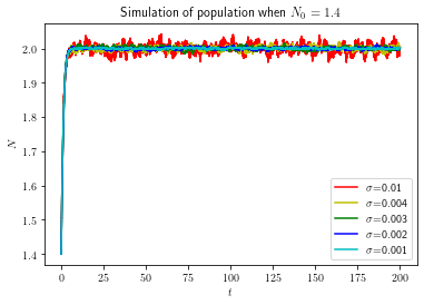
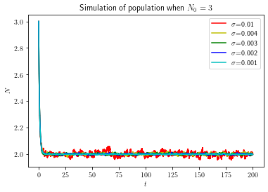
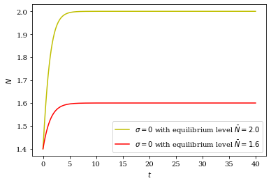
We first provide numerical examples for the population state. The quantity $\bar{N}$ in $f(x)$ represents the equilibrium level of the population, to which the population should converge as $t$ approaches infinity. Figure 1 depicts the movement of $N$ against $t$ for different initial values $N_{0}=$ 1.4 and 3 with $\bar{N}=2$, along with varying values of $\sigma$, representing different levels of volatility and fluctuation. Notably, all scenarios demonstrate quick convergence, and the red curves in both subfigures cover all the other curves due to their largest magnitudes of fluctuations. This observation highlights the significant impact of $\sigma$ on the population dynamics.

Figure 1. Simulation of population with $\alpha$= 0.5, $M=3$ and $\bar{N}=2.0$.

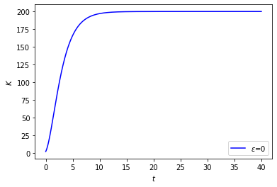
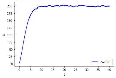
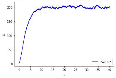
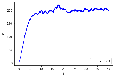
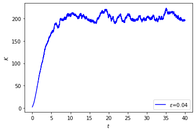
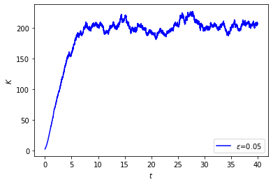
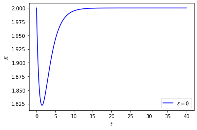
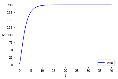
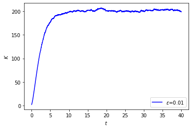
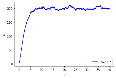
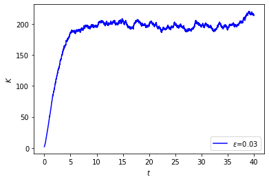
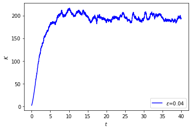
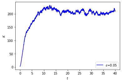
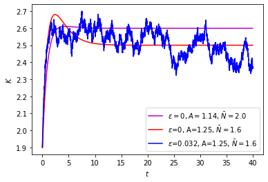
As for the capital dynamics, we first consider a scenario where the production function is dominant due to a very large coefficient $A$, indicating high production efficiency. In our simulations, given an initial value for capital (which is 2 in our simulation), the production function drives the behavior of capital, leading to its increase regardless of population movement. Capital also converges to an equilibrium in a manner similar to population, as shown in Figure 2. If we ignore production (i.e., $A=0$), the capital decreases significantly with the sole contribution from consumption. Hence, a phase transition behavior is expected for intermediate values of $A$.

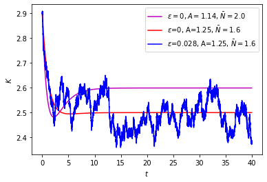
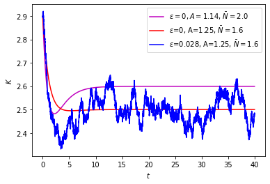
Meanwhile, it is crucial in our study whether the population is increasing or decreasing to the equilibrium level. The total consumption remains approximately proportional to capital due to the control effect $c=(u^{\prime}_{1})^{-1}(v_{k})\simeq\frac{K}{N}$. If the population is relatively small at the beginning and increases towards the equilibrium level, when $A$ falls within a critical region, a small initial value of $N$ leads to a small value for the production function initially, after subtracting the total consumption it will lead to the decay of capital. Subsequently, we may expect the capital to increase due to the population growth and reduced total consumption, resulting in an undershoot behavior. Conversely, if the initial population is relatively large and decreases towards equilibrium, we may expect an overshoot behavior in capital. This model motivates an explanation of a sharp economic growth after a body boom. These two types of capital behavior illustrate the potential pitfalls in anticipating economic trends. For instance, a decrease in capital might be perceived negatively, but it could actually be the turning point for the economy. In a certain sense, in order to understand the economy, one has to consider both the population and capital dynamics. By carefully considering the interactions between production function, population, and consumption, we gain insights into the dynamic behavior of the economy, shedding light on potential economic trends and the need for cautious interpretation of observed phenomena.

To verify our observations, we present various numerical illustrations on the movement of the capital. We have previously observed the rapid convergence of population in Figure 1 regardless of the value of $\sigma$. Therefore, in the following illustrations, we set $\sigma=0$ to demonstrate the capital dynamics more clearly. Now, let us describe the other parameter settings as follows: the population deterministically increase or decrease from initial value $N_{0}$ to the equilibrium level $\bar{N}=2$; $\epsilon$ takes values from 0 to 0.05 at an 0.01 interval. We present the simulations of $K(t)$ with initial value $K_{0}=2$ in Figures 2, 3, 4 and 5 when the pair of parameters $(N_{0},A)=(1.4,10),(1.4,1),(3,10),(3,1)$, respectively. We observe that when $A=10$, $K(t)$ exhibits an increasing trend regardless of the values of $N_{0}$ and $\epsilon$. On the other hand, when $A=1$, which actually falls into a critical region, we observe clear undershoot (resp. overshoot) behavior as long as $\epsilon$ below 0.03 when there is an increasing (resp. decreasing) trend towards equilibrium for population. However, such behavior becomes unidentifiable when $\epsilon$ is above 0.03 due to the large fluctuations, regardless of the population trend.

Figure 2. Simulation of capital when $(N_{0},A)=(1.4,10)$, $K_{0}=2$ and $\epsilon=0,\ 0.01,\ 0.02,\ 0.03,\ 0.04,\ 0.05$.

Figure 3. Simulation of capital when $(N_{0},A)=(1.4,1)$, $K_{0}=2$ and $\epsilon=0,\ 0.01,\ 0.02,\ 0.03,\ 0.04,\ 0.05$

Figure 4. Simulation of capital when $(N_{0},A)=(3,10)$, $K_{0}=2$ and $\epsilon=0,\ 0.01,\ 0.02,\ 0.03,\ 0.04,\ 0.05$.

Figure 5. Simulation of capital when $(N_{0},A)=(3,1)$, $K_{0}=2$ and $\epsilon=0,\ 0.01,\ 0.02,\ 0.03,\ 0.04,\ 0.05$.

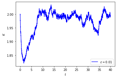
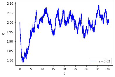
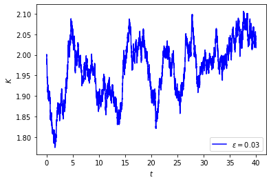
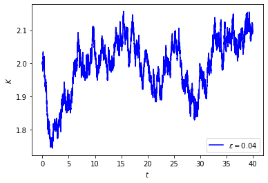
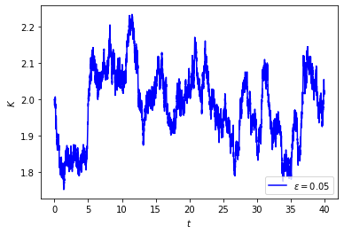
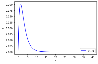
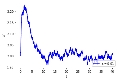
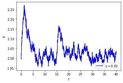
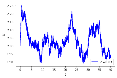
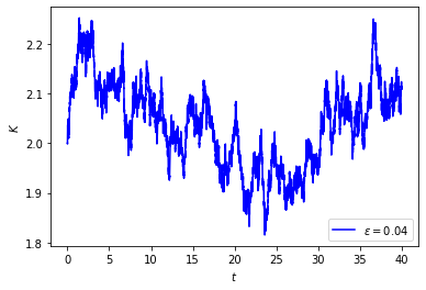
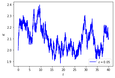
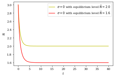
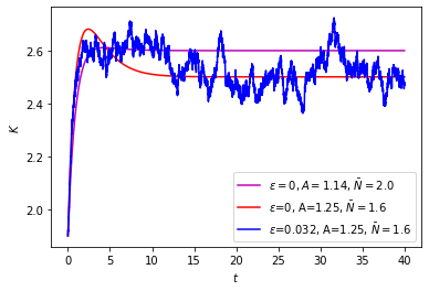
To conclude this section, we further investigate the effect of the random noise; namely its existence hinders our ability to tell whether the overshoot or undershoot behavior is present for $K(t)$. To do so, we conduct two sets of simulations and plot their respective results in Figures 6 to 9. In these figures, we first consider two populations with the same initial value but different equilibrium, with corresponding parameters specified in each plot. We then plot the paths of $K$ in Figure 7 and Figure 9 under the different dynamics of populations. We can see that if we are only given the development of the capital, it is challenging for us to determine whether the red line or the violet line of population traces represent the true underlying population, especially when the random noise is significant, hence increasing the difficulty to identify the overshoot (resp. undershoot) behavior of capital correctly. That is, the presence of random noise complicates the interpretation of the asymptotic behavior of the capital, leading to potential misunderstandings. Therefore, the effect of random fluctuations should be carefully considered when we analyze the behavior of the capital process and draw conclusions based solely on observed data.

Figure 6. Simulation of population with initial value $N_{0}=$3 and equilibrium levels $\bar{N}=$1.6 and $\bar{N}=$2.

Figure 7. Simulation of capital under different population dynamics when $N_{0}=3,K_{0}=1.9$.

Figure 8. Simulation of population with initial value $N_{0}=$1.4 and equilibrium levels $\bar{N}=$1.6 and $\bar{N}=$2.

Figure 9. Simulation of capital evolution under different population dynamics.

4. Unique existence of the classical solution of (2.5) in the local Hölder space

We show the existence in Subsection 4.1 and uniqueness in Subsection 4.2 for Problem (2.5) with smooth input $\psi$. The main difficulty encountered here is the exponential growth of the coefficients of Equation (4.2), this prevents us from obtaining a global Schauder estimates to establish a solution, and it is also not possible to use the classical maximum principle to conclude uniqueness. Since the solution is expected to be unbounded on the whole space, our main idea is to multiply the solution by an appropriate spatial weight so that the weighted solution is bounded. Then, we can apply the maximum principle to the weighted solution to derive $L^{\infty}$ estimates and uniqueness.

One should note that the $L^{\infty}$ bounds obtained in this section do not provide the crucial non-trivial lower bounds of the solutions to (2.5), which is essential for the well-posedness of the nonlinear problem, and this will be the main objective of Section 5.

We now state the existence and uniqueness results given in this section:

Theorem 4.1.

Let $\psi\in{C^{\infty}([0,T]\times\mathbb{R}^{2}_{+})}$ such that

(i) when $\beta\geq\gamma$, $~{}\psi(t,K,N)\geq c_{0}^{\gamma}\left(\frac{N}{K}\right)^{\gamma}~{}$ for a positive constant $c_{0}$;

(ii) when $\beta<\gamma$, $~{}\psi(t,K,N)\geq C_{3}\left(\frac{N}{K}\right)^{\beta}\left(C_{4}\left(\frac{N}{K}\right)^{\beta-1}+C_{5}\right)^{\frac{\gamma-\beta}{\beta-1}}~{}$ for some positive constants $C_{3}$, $C_{4}$

and $C_{5}$.
Then there is a unique classical solution $\lambda$ to (2.5) satisfying

(4.1) $$|\lambda(t,K,N)|\leq B\left(\left(\frac{N}{K}\right)^{\beta_{1}}+\left(\frac{N}{K}\right)^{\gamma_{1}}\right),~{}t\in[0,T],$$

for some $B>0$ and $0<\beta_{1},\gamma_{1}<1$. Furthermore, $\lambda\in C^{1+\frac{\alpha}{2},2+\alpha}_{loc}([0,T]\times\mathbb{R}^{2}_{+})$ for any $0<\alpha<1$.

For this theorem, any constants $c_{0}$, $C_{3}$, $C_{4}$ and $C_{5}$ suffice for the claim of the unique existence of the solution.

4.1. $L^{\infty}$ a priori estimates and existence of a solution of the linearized equation (2.5)

For the linearized equation (2.5), we try to use some classical tools of parabolic equations directly to obtain a regular solution. To do so, we want to first transform (2.5) into a uniformly parabolic equation. Precisely, we apply the transformation $K=e^{x}$, $N=e^{y}$, $x,y\in\mathbb{R}$, and denote $\tilde{\lambda}(t,x,y)={\lambda}(t,e^{x},e^{y})$, we then obtain the following equation for $\tilde{\lambda}$ from Equation (2.5):

(4.2) $$\left\{\begin{aligned} \tilde{\lambda}_{t}&+\left(-e^{y-x}j(\psi(t,e^{x},e^{y}))+Ae^{(y-x)(1-\beta)}+\frac{1}{2}\epsilon^{2}\right)\tilde{\lambda}_{x}+\left(\frac{f(e^{y})}{e^{y}}-\frac{1}{2}\sigma^{2}\right)\tilde{\lambda}_{y}\\ &+\frac{1}{2}\epsilon^{2}\tilde{\lambda}_{xx}+\frac{1}{2}\sigma^{2}\tilde{\lambda}_{yy}+A\beta e^{(y-x)(1-\beta)}\tilde{\lambda}=0,~{}x,y\in\mathbb{R},~{}t\in[0,T),\\ &\tilde{\lambda}(T,x,y)=\tilde{u}_{2}(e^{y-x})\quad(\textrm{its rate is asymptotically equal to }e^{\gamma(y-x)}),\end{aligned}\right.$$

where $\tilde{u}_{2}(z)=u^{\prime}_{2}(\frac{1}{z})$. We use $w:=\frac{\tilde{\lambda}}{\rho}$ to transform Equation (4.2), where the auxiliary function $\rho=e^{(\beta+\theta)(y-x)}+e^{\gamma(y-x)}>0$ and $\theta$ is a positive number. We then obtain:

(4.3) $$\left\{\begin{aligned} &w_{t}+\left({-e^{y-x}j(\psi)}+Ae^{(y-x)(1-\beta)}+\frac{1}{2}\epsilon^{2}+\epsilon^{2}\frac{\rho_{x}}{\rho}\right)w_{x}+\left(\frac{f(e^{y})}{e^{y}}-\frac{1}{2}\sigma^{2}+\sigma^{2}\frac{\rho_{y}}{\rho}\right)w_{y}\\ &\quad+\frac{1}{2}\epsilon^{2}w_{xx}+\frac{1}{2}\sigma^{2}w_{yy}+\left[\left({\color[rgb]{1,0,0}\definecolor[named]{pgfstrokecolor}{rgb}{1,0,0}-e^{y-x}j(\psi)}+{\color[rgb]{1,0,0}\definecolor[named]{pgfstrokecolor}{rgb}{1,0,0}Ae^{(y-x)(1-\beta)}}+\frac{1}{2}\epsilon^{2}\right)\frac{\rho_{x}}{\rho}\right.\\ &\left.\quad+\left(\frac{f(e^{y})}{e^{y}}-\frac{1}{2}\sigma^{2}\right)\frac{\rho_{y}}{\rho}+\frac{1}{2}\epsilon^{2}\frac{\rho_{xx}}{\rho}+\frac{1}{2}\sigma^{2}\frac{\rho_{yy}}{\rho}+{\color[rgb]{1,0,0}\definecolor[named]{pgfstrokecolor}{rgb}{1,0,0}A\beta e^{(y-x)(1-\beta)}}\right]w=0,~{}\textrm{for}~{}(x,y)\in\mathbb{R}^{2},t\in[0,T],\\ &w(T,x,y)=\frac{\tilde{u}_{2}(e^{y-x})}{\rho}.\end{aligned}\right.$$

The auxiliary function $\rho$ serves as a weight function and it captures the growth rate of $\tilde{\lambda}$ (the solution of Equation (4.2)) in order to make $w=\frac{\tilde{\lambda}}{\rho}$ as a bounded function. To derive the Schauder estimate for $w$, we shall apply an approximation scheme that truncates the unbounded coefficients. The key is to obtain the $L^{\infty}$ estimate uniformly in these approximate solutions so that we can extract a convergent subsequence from the approximate solutions.

To apply the maximum principle, we need to ensure an upper bound for the coefficient of zeroth-order term of $w$. To this end, it is easy to see that we only need to provide an upper bound for the sum of red terms in (4.3), i.e., $-e^{y-x}j(\psi)\frac{\rho_{x}}{\rho}+Ae^{(y-x)(1-\beta)}\frac{\rho_{x}+\beta\rho}{\rho}$ since all the other terms are already bounded. It could be done by a detailed calculation with this particular choice of $\rho$ using the bounds on $\psi$ stated in Theorem 4.1 and the bound on $j(x)$ in (2.3) by considering the cases $\beta\geq\gamma$ and $\beta<\gamma$ separately, one can refer to [25, Section 3.2] for more detailed calculations, and we omit the details here. Hence, we obtain that the coefficient of zeroth-order term of $w$ is bounded from above by some constant $M$ depending on given parameters as follows:

(4.4) $$\left(-e^{y-x}j(\psi)+Ae^{(y-x)(1-\beta)}+\frac{1}{2}\epsilon^{2}\right)\frac{\rho_{x}}{\rho}+\left(\frac{f(e^{y})}{e^{y}}-\frac{1}{2}\sigma^{2}\right)\frac{\rho_{y}}{\rho}$$

$$\quad+\frac{1}{2}\epsilon^{2}\frac{\rho_{xx}}{\rho}+\frac{1}{2}\sigma^{2}\frac{\rho_{yy}}{\rho}+A\beta e^{(y-x)(1-\beta)}\leq M(\theta,\beta,\gamma,C_{f},A,\epsilon,\sigma,a_{1},c_{0}).$$

We can then consider the approximate solution $w^{m}$ to the following approximate equation for Equation (4.3) and derive its uniform $L^{\infty}$ bound being independent of $m$ with the aid of the classical maximum principle:

(4.5) $$\left\{\begin{aligned} w^{m}_{t}&+\left(-e^{y-x}j(\psi)+Ae^{(y-x)(1-\beta)}+\frac{1}{2}\epsilon^{2}+\epsilon^{2}\frac{\rho_{x}}{\rho}\right)\xi_{m}w^{m}_{x}\\ &+\left(\frac{f(e^{y})}{e^{y}}-\frac{1}{2}\sigma^{2}+\sigma^{2}\frac{\rho_{y}}{\rho}\right)\xi_{m}w^{m}_{y}+\frac{1}{2}\epsilon^{2}w^{m}_{xx}+\frac{1}{2}\sigma^{2}w^{m}_{yy}\\ &+\left((-e^{y-x}j(\psi)+Ae^{(y-x)(1-\beta)}+\frac{1}{2}\epsilon^{2})\frac{\rho_{x}}{\rho}\right.\\ &\left.\quad+\left(\frac{f(e^{y})}{e^{y}}-\frac{1}{2}\sigma^{2}\right)\frac{\rho_{y}}{\rho}+\frac{1}{2}\epsilon^{2}\frac{\rho_{xx}}{\rho}+\frac{1}{2}\sigma^{2}\frac{\rho_{yy}}{\rho}+A\beta e^{(y-x)(1-\beta)}\right)\xi_{m}w^{m}=0,\\ &w^{m}(T,x,y)=\frac{\tilde{u}_{2}(e^{y-x})}{\rho},\end{aligned}\right.$$

where $\xi_{m}$ for $m\geq$1 is a sequence of smooth cutoff functions such that $\xi_{m}=1$ on the ball $\mathcal{B}_{\frac{m}{2}}(0)$ and vanishes outside the ball $\mathcal{B}_{m}(0)$ with bounded derivatives whose bounds independent of $m$. The unique existence of solution $w_{m}$ in $C^{1+\frac{\alpha}{2},2+\alpha}([0,T]\times\mathbb{R}^{2})$ for Equation (4.5) is standard as the coefficients are all bounded, being at least Lipschitz continuous, and the terminal data is $C^{3}$. It is also clear that the coefficient of the zeroth-order term of Equation (4.5) is bounded from above by the same bound $M=M(\theta,\beta,\gamma,C_{f},A,\epsilon,\sigma,a_{1},c_{0})$ in (4.4) which is independent of $m$. Hence, it follows from the comparison principle that, by first comparing with 0, we see that $w^{m}>0$. Clearly, $w$ is bounded as $0<w(T,x,y)\leq a_{3}$ due to Assumption IV on $u_{2}$ (see also (5.7)). Then comparing with $e^{M(T-t)}M_{1}$ such that $M_{1}:=\sup_{\mathbb{R}^{2}}\frac{\tilde{u}_{2}(e^{y-x})}{\rho}$, we also have

(4.6) $$0<w^{m}\leq e^{M(T-t)}M_{1},~{}M=M(\theta,\beta,\gamma,C_{f},A,\epsilon,\sigma,a_{1},c_{0}).$$

Using the classical interior Schauder estimates (cf. [14]), and the uniform $L^{\infty}$ bound of $w^{m}$ we obtained in (4.6), we can use a diagonal argument to find a subsequence $\{w^{m_{k}}\}_{k=0}^{\infty}$ such that $w^{m_{k}}$ converge to some $w$ in $C^{1+\frac{\alpha}{2},2+\alpha}_{loc}([0,T]\times\mathbb{R}^{2})$ for any $0<\alpha<1$. We can now conclude that Equation (4.3), and so, Equation (4.2) has a classical solution in $C^{1+\frac{\alpha}{2},2+\alpha}_{loc}([0,T]\times\mathbb{R}^{2})$ for any $\alpha<1$. Besides, it is smooth as long as $j$, $\psi$, and $f$ are smooth by the standard regularity theory; see [14] for instance.

Remark 4.2.

The conventional maximum principle helps in establishing an upper bound but not so for getting a more precise lower bound other than the trivial bound 0, without which it is impossible to ensure the well-posedness of the nonlinear problem (2.2). We shall obtain more accurate lower and upper bounds for the solution $\lambda$ below in next Section 5 through Theorem 5.1 and Theorem 5.2.

4.2. A modified maximum principle for the linearized equation (4.2) and uniqueness of its solution

In this section, we aim to establish the uniqueness of the classical solution for Equation (4.2) within a certain function class. For this purpose, we need a customized maximum principle to handle the growth rate. We begin with a lemma asserting that if we already have the control, uniformly in time for the solution at the far field, then the maximum principle holds.

Lemma 4.3.

Consider the parabolic operator

(4.7) $$Lu:=\sum_{i,j=1}^{n}a_{ij}(t,x)\frac{\partial^{2}u}{\partial x_{i}\partial x_{j}}+\sum_{i=1}^{n}b_{i}(t,x)\frac{\partial u}{\partial x_{i}}+c(t,x)u-\frac{\partial u}{\partial t},$$

for $(t,x)\in(0,T]\times\mathbb{R}^{n}$. Assume that $a_{ij}$, $b_{i}$ and $c$ are continuous for $i,j=1,\cdots,n$. Moreover, $c$ is assumed to be bounded from above. If $Lu\leq 0$ on $(0,T]\times\mathbb{R}^{n}$, $u(0,x)\geq 0$ on $\mathbb{R}^{n}$ and

(4.8) $$\liminf_{|x|\to\infty}u(t,x)\geq 0$$

uniformly in $t\in[0,T]$, then $u(t,x)\geq 0$ on $[0,T]\times\mathbb{R}^{n}$.

This lemma is standard, we refer to [14, Section 2.4, Lemma 5].

Theorem 4.4 (Maximum principle).

Let $\psi$ satisfy the condition specified in Theorem 4.1. Assume that $\tilde{\lambda}$ is a classical solution of Equation ${\eqref{eq: equation for tilde lamba}}_{1}$, and $|\tilde{\lambda}(t,x,y)|\leq B(e^{\beta_{1}(y-x)}+e^{\gamma_{1}(y-x)})$ for all $(x,y)\in\mathbb{R}^{2}$, $t\in[0,T]$ for some constants $0<\beta_{1},\gamma_{1}<1$ and $B>0$. If $\tilde{\lambda}(T,x,y)\geq 0$ on $\mathbb{R}^{2}$, then $\tilde{\lambda}(t,x,y)\geq 0$ on $[0,T]\times\mathbb{R}^{2}$.

Proof.

The validity of our claim relies on a suitable choice of a weight function $\rho$, which should have faster growth at infinity than those assumed for $\tilde{\lambda}$. Let $\rho=e^{-x+2y}+e^{x-y}+e^{-x+y}+e^{-x-y}$. Consider $w=\frac{\tilde{\lambda}}{\rho}$ which satisfies ${\eqref{eq: the equation of w}}_{1}$ for this new choice $\rho$. After some elaborate calculations (cf. [25, Pooof of Theorem 3.3.1]), one can show that the coefficient of the zeroth-order term in ${\eqref{eq: the equation of w}}_{1}$ is still bounded from above no matter $\beta\geq\gamma$ or $\beta<\gamma$; moreover

(4.9) $$\lim_{R\to\infty}\sup_{|x|+|y|\geq R}|w|\to 0~{}\textrm{uniformly in $t\in[0,T]$},$$

due to the choice of this new $\rho$ and the bound on $\tilde{\lambda}$ assumed in the statement, i.e., $|\tilde{\lambda}(t,x,y)|\leq B(e^{\beta_{1}(y-x)}+e^{\gamma_{1}(y-x)})$. Applying Lemma 4.3 (after a reversal of time), we have $w\geq 0$, so is $\tilde{\lambda}$. ∎

Remark 4.5.

In fact Theorem 4.4 remains valid under a weaker condition $\tilde{\lambda}(t,x,y)\geq-B(e^{\beta_{1}(y-x)}+e^{\gamma_{1}(y-x)})$ upon Lemma 4.3.

Remark 4.6.

The maximum principle provided in Theorem 4.4 is designed for our parabolic operator with exponential growth coefficients, for which we need a more stringent growth rate on the solution compared with the classical result. That is, if the growth rates of the coefficients are not so rapid, then the maximum principle holds for a broader class of functions. In particular, if the coefficients $a_{ij}$’s of the parabolic operator in (4.7) are bounded, $b_{i}$’s are of at most linear growth rate, and $c$ is of at most quadratic growth, then the maximum principle holds for the class of solutions with at most $e^{k|x|^{2}}$ (for any $k>0$) growth rate in $x$; see [14, Section 2.4, Theorem 9 and Theorem 10].

Corollary 4.7 (Uniqueness of the classical solution).

There exists at most one classical solution to the Cauchy problem (4.2) satisfying

$$|\tilde{\lambda}(t,x,y)|\leq B(e^{\beta_{1}(y-x)}+e^{\gamma_{1}(y-x)}),~{}t\in[0,T],$$

for some constants $B>0$ and $0<\beta_{1},\gamma_{1}<1$.

Proof.

To show the uniqueness, we only need to show $\tilde{\lambda}=0$ when the terminal data $\tilde{u}_{2}$ in the second equation of Problem $\eqref{eq: equation for tilde lamba}$ is replaced by 0. We then apply Theorem 4.4 for $\tilde{\lambda}$ and $-\tilde{\lambda}$ to deduce that. ∎

5. Refined pointwise estimates for the solution to the linearized problem (2.5)

We derive the refined pointwise lower and upper estimates, which seem almost optimal for the solution $\lambda$ to the linearized equation (2.5). In particular, we shall establish a crucial lower bound for solutions to (2.5) that enables the application of a fixed point argument to solve (2.2). To achieve this, we employ a combination of probabilistic and analytic methodologies, combining the strengths of both approaches.

The main tools of use are the celebrated Feynman-Kac formula with a delicate stochastic analysis for a pair of partially coupled diffusion processes with non-Lipschitz driving coefficients associated with the infinitesimal generator of Equation (2.5) and a sophisticated use of Hölder’s and reverse Hölder’s inequalities. The main results in this section are the following.

Theorem 5.1 (Pointwise estimates when $\beta\geq\gamma$).

Let $\beta$, $\gamma$ $\in(0,1)$ such that $\beta\geq\gamma$. Let the input function $\psi$ be a continuous function satisfying $\psi(t,K,N)\geq c_{0}^{\gamma}\left(\frac{N}{K}\right)^{\gamma}$ for some positive constant $c_{0}$ which is specified in (5.9). Assume that $\lambda\in C^{1,2}([0,T]\times\mathbb{R}_{+}^{2})$ is a classical solution of the linearized problem (2.5). Under Assumptions III and IV in Section 1.2, the solution $\lambda$ satisfies

$$c_{0}^{\gamma}\left(\frac{N}{K}\right)^{\gamma}\leq\lambda(t,K,N)\leq C_{1}\left(\frac{N}{K}\right)^{\gamma}+C_{2}\left(\frac{N}{K}\right)^{\beta},$$

where the positive constants $C_{1}$ and $C_{2}$ are given in (5.14) and (5.15) when $\gamma\leq 2\beta-1$ or in (5.25) when $\gamma>2\beta-1$.

Theorem 5.2 (Pointwise estimates for $\beta<\gamma$).

Let $\beta$, $\gamma$ $\in(0,1)$ such that $\beta<\gamma$. Let the input function $\psi$ be a continuous function satisfying $\psi(t,K,N)\geq C_{3}\left(\frac{N}{K}\right)^{\beta}\left(C_{4}\left(\frac{N}{K}\right)^{\beta-1}+C_{5}\right)^{\frac{\gamma-\beta}{\beta-1}}$. Assume that $\lambda\in C^{1,2}([0,T]\times\mathbb{R}_{+}^{2})$ is a classical solution of the linearized problem (2.5). Under Assumptions III and IV in Section 1.2, then the solution $\lambda$ satisfies

$$C_{3}\left(\frac{N}{K}\right)^{\beta}\left(C_{4}\left(\frac{N}{K}\right)^{\beta-1}+C_{5}\right)^{\frac{\gamma-\beta}{\beta-1}}\leq\lambda(t,K,N)\leq C_{6}\left(\frac{N}{K}\right)^{\gamma},$$

where the positive constants $C_{3},C_{4}$ and $C_{5}$ are given in (5.33), and $C_{6}$ is given in (5.38).

The proof of Theorem 5.1 relies on Lemma 5.6 (providing the lower bound when $\beta\geq\gamma$), Lemma 5.9, and Lemma 5.11 (together providing the upper bound when $\beta\geq\gamma$). On the other hand, the proof of Theorem 5.2 involves Lemma 5.13 (giving the lower bound when $\beta<\gamma$) and Lemma 5.15 (giving the upper bound when $\beta<\gamma$).

To summarize, in Subsection 5.1 we derive a Feynman-Kac representation for the solution to Problem (2.5). In Subsections 5.2 and 5.3, we establish the lower and upper bounds when $\beta\geq\gamma$, respectively; while in Subsection 5.4, we derive the lower and upper bounds in the case $\beta<\gamma$. All of them rely on the Feynman-Kac representation in Subsection 5.1.

5.1. Feynman-Kac representation of the solution to the linearized problem (2.5)

Given the existence of the solution $\lambda$ of Equation (2.5), we give its solution formula. To this end, we adopt the celebrated Feynman-Kac formula to express it through some properly chosen diffusion processes. It is more feasible for us to derive pointwise estimates, particularly the more critical lower bounds.

Specifically, we first define two processes $X_{1}$ and $X_{2}$, which are associated with the infinitesimal generators of Equation (2.5), with which the corresponding Feynman-Kac formulas can be derived. We consider

(5.1) $$\left\{\begin{aligned} dX_{1}(s)=&\left[AX_{2}^{1-\beta}(s)X_{1}^{\beta}(s)-X_{2}(s)j\left(\psi\left(s,X_{1}(s),X_{2}(s)\right)\right)+{\epsilon}^{2}X_{1}(s)\right]ds+{\epsilon}X_{1}(s)dB_{1}(s),\\ X_{1}(t)=&K,\end{aligned}\right.$$

(5.2) $$\left\{\begin{aligned} dX_{2}(s)&=f(X_{2}(s))ds+{{\sigma}}X_{2}(s)dB_{2}(s),\\ X_{2}(t)&=N,\end{aligned}\right.$$

where $B_{1}(s)$ and $B_{2}(s)$ are two independent Brownian motions on some suitable probability space. There is a unique process $X_{2}$ satisfying (5.2) since $f(x)$ is Lipschitz continuous. Moreover, since

$$dX_{2}(s) \geq-C_{f}X_{2}ds+{{\sigma}}X_{2}(s)dB_{2}(s),\quad X_{2}(t)=N>0,$$

we deduce from the comparison principle that $X_{2}(s)>0$ for all $s\in[t,T]$. For the process $X_{1}$, it is not obvious that it has a solution, so we need to first show the solvability of $X_{1}$.

Lemma 5.3 (Existence of process $X_{1}$).

There exists a solution $X_{1}$ of (5.1).

To prove this, we adopt the idea of considering the stochastic differential equation (SDE) for $X_{1}^{1-\beta}$, which is motivated by the Bernoulli differential equation. Importantly, the corresponding SDE is indeed “almost” linear. The proof of Lemma 5.3 will be provided in Appendix A. Applying the Feynman-Kac formula, we can express $\lambda$ in an expectation form in terms of the processes $X_{1}$ and $X_{2}$ as follows.

Lemma 5.4 (Feynman-Kac formula for $\lambda$).

For $\lambda$, the classical solution to Problem (2.5), we can write

(5.3) $$\lambda(t,K,N)=\mathbb{E}\left[e^{\int_{t}^{T}A\beta(X_{2}(\tau))^{1-\beta}(X_{1}(\tau))^{\beta-1}d\tau}u^{\prime}_{2}\left(\frac{X_{1}(T)}{X_{2}(T)}\right)\right].$$

Indeed, by considering $Y(s)=e^{\int_{t}^{s}A\beta(X_{2}(\tau))^{1-\beta}(X_{1}(\tau))^{\beta-1}d\tau}\lambda(s,X_{1}(s),X_{2}(s))$, we can establish this Lemma 5.4, and the details are in Appendix A. We mainly aim to utilize (5.3) to derive both lower and upper pointwise bounds for $\lambda(t,K,N)$. Motivated by the expression (5.3), to estimate $\lambda(t,K,N)$, we consider the process

(5.4) $$G(s) :=e^{\int_{t}^{s}A\beta(X_{2}(\tau))^{1-\beta}(X_{1}(\tau))^{\beta-1}d\tau}u^{\prime}_{2}\left(\frac{X_{1}(s)}{X_{2}(s)}\right)=e^{\int_{t}^{s}A\beta(X_{2}(\tau))^{1-\beta}(X_{1}(\tau))^{\beta-1}d\tau}\tilde{u}_{2}\left(\frac{X_{2}(s)}{X_{1}(s)}\right),$$

where $\tilde{u}_{2}(x)=u^{\prime}_{2}(\frac{1}{x})$, since we have $\lambda(t,K,N)=\mathbb{E}[G(T)]$. Our main goal is then to estimate $\mathbb{E}[G(T)]$ by studying the process $G(s)$ and other related processes. A direct computation using (5.1) and (5.2) shows that

(5.5) $$d\left(\frac{X_{2}}{X_{1}}\right) =\frac{1}{X_{1}}dX_{2}+X_{2}d\left(\frac{1}{X_{1}}\right)+d(X_{2})d\left(\frac{1}{X_{1}}\right)$$

$$=\frac{1}{X_{1}}\left(f(X_{2})ds+{{\sigma}}X_{2}dB_{2}\right)-\frac{X_{2}}{X_{1}^{2}}(AX_{2}^{1-\beta}X_{1}^{\beta}-X_{2}j(\psi)+\epsilon^{2}X_{1})ds+\epsilon^{2}X_{2}X_{1}^{-1}ds-\epsilon\frac{X_{2}}{X_{1}}dB_{1}$$

$$=\frac{1}{X_{1}}f(X_{2})ds-\left(A\left(\frac{X_{2}}{X_{1}}\right)^{2-\beta}-\left(\frac{X_{2}}{X_{1}}\right)^{2}j(\psi)\right)ds+{{\sigma}}\frac{X_{2}}{X_{1}}dB_{2}(s)-\epsilon\frac{X_{2}}{X_{1}}dB_{1}(s).$$

From above, the dynamics of $G$ can be easily obtained, and it will be used to derive various useful estimates. We have

Proposition 5.5.

For $0<s<T$,

(5.6) $$dG(s) =A\left(\beta-\frac{\tilde{u}_{2}^{\prime}\left(\frac{X_{2}}{X_{1}}\right)}{\tilde{u}_{2}\left(\frac{X_{2}}{X_{1}}\right)}\cdot\frac{X_{2}}{X_{1}}\right)\cdot\left(\frac{X_{2}}{X_{1}}\right)^{1-\beta}Gds$$

$$\quad+e^{\int_{t}^{s}A\beta(X_{2}(\tau))^{1-\beta}(X_{1}(\tau))^{\beta-1}d\tau}\tilde{u}_{2}^{\prime}\left(\frac{X_{2}}{X_{1}}\right)\left[\frac{1}{X_{1}}f(X_{2})ds+\left(\frac{X_{2}}{X_{1}}\right)^{2}j(\psi)ds\right]$$

$$\quad+e^{\int_{t}^{s}A\beta(X_{2}(\tau))^{1-\beta}(X_{1}(\tau))^{\beta-1}d\tau}\left[\frac{1}{2}\tilde{u}_{2}^{\prime\prime}\left(\frac{X_{2}}{X_{1}}\right)\left(\frac{X_{2}}{X_{1}}\right)^{2}({{\sigma}^{2}}+{\epsilon}^{2})ds\right]$$

$$\quad+e^{\int_{t}^{s}A\beta(X_{2}(\tau))^{1-\beta}(X_{1}(\tau))^{\beta-1}d\tau}\tilde{u}_{2}^{\prime}\left(\frac{X_{2}}{X_{1}}\right)\left(\frac{X_{2}}{X_{1}}\right)\left({{\sigma}}dB_{2}-\epsilon dB_{1}\right).$$

We note that it follows from Assumption IV (i.e., conditions on $u_{2}$) that $\tilde{u}_{2}$ satisfies the following conditions:

(5.7) $$a_{2}x^{\gamma}\leq\tilde{u}_{2}(x)\leq a_{3}x^{\gamma},~{}\min\{\beta,\gamma\}\tilde{u}_{2}(x)\leq x{\tilde{u}_{2}^{\prime}}(x)\leq\max\{\beta,\gamma\}\tilde{u}_{2}(x),~{}\tilde{a}_{4}\tilde{u}_{2}(x)\leq x^{2}\tilde{u}_{2}^{\prime\prime}(x)\leq\tilde{a}_{5}\tilde{u}_{2}(x),$$

where

(5.8) $$\tilde{a}_{4}=a_{4}-2\max\{\beta,\gamma\}\textrm{ and }\tilde{a}_{5}=a_{5}-2\min\{\beta,\gamma\}$$

are both constants.

5.2. Lower bound for the solution in the case $\beta\geq\gamma$

This section derives a lower bound for the solution $\lambda$ to the linearized problem (2.5) when $\beta\geq\gamma$. Our main result is:

Lemma 5.6 (Lower bound for $\lambda$).

Under the same assumptions stated in Theorem 5.1, we have

$$\lambda(t,K,N)=\mathbb{E}[G(T)]\geq a_{2}e^{(-C_{f}\beta+\frac{\tilde{a}_{4}}{2}({\sigma}^{2}+\epsilon^{2}))(T-t)}\left(\frac{N}{K}\right)^{\gamma}\geq c_{0}^{\gamma}\left(\frac{N}{K}\right)^{\gamma},$$

where the constant

(5.9) $$c_{0}=\min{\left\{a_{2}^{\frac{1}{\gamma}},a_{2}^{\frac{1}{\gamma}}e^{{(-C_{f}\beta+\frac{\tilde{a}_{4}}{2}({\sigma}^{2}+\epsilon^{2}))T}/{\gamma}}\right\}}.$$

Proof.

It follows from (5.6), conditions (5.7), Assumption II, $j(\psi)>0$ and $\beta\geq\gamma$ that we have

$$dG(s)\geq\tilde{a}G(s)ds+e^{\int_{t}^{s}A\beta(X_{2}(\tau))^{1-\beta}(X_{1}(\tau))^{\beta-1}d\tau}\tilde{u}_{2}^{\prime}\left(\frac{X_{2}}{X_{1}}\right)\frac{X_{2}}{X_{1}}({{\sigma}}dB_{2}-\epsilon dB_{1}),$$

for the constant $\tilde{a}:=-C_{f}\beta+\frac{\tilde{a}_{4}}{2}({\sigma}^{2}+\epsilon^{2})$. Integrating from $t$ to $s$ yields

$$G(s)-G(t)\geq \int_{t}^{s}\tilde{a}G(\tau)d\tau+\int_{t}^{s}e^{\int_{t}^{\tau}A\beta(X_{2}(\tau))^{1-\beta}(X_{1}(\tau))^{\beta-1}d\tau}\tilde{u}_{2}^{\prime}\left(\frac{X_{2}(\tau)}{X_{1}(\tau)}\right)\frac{X_{2}}{X_{1}}(\tau)({{\sigma}}dB_{2}-\epsilon dB_{1}).$$

Taking expectations on both sides and using the initial conditions $\eqref{eq:process of X_1}_{2}$ and $\eqref{eq:process of X_2}_{2}$, we have

$$\mathbb{E}[G(s)]-a_{2}\left(\frac{N}{K}\right)^{\gamma}\geq\mathbb{E}[G(s)-G(t)]$$

$$\geq \mathbb{E}\left[\int_{t}^{s}\tilde{a}G(\tau)d\tau+\int_{t}^{s}e^{\int_{t}^{\tau}A\beta\left(\frac{X_{2}}{X_{1}}(\tau)\right)^{1-\beta}d\tau}\tilde{u}_{2}^{\prime}\left(\frac{X_{2}(\tau)}{X_{1}(\tau)}\right)\left(\frac{X_{2}(\tau)}{X_{1}(\tau)}\right)({{\sigma}}dB_{2}-\epsilon dB_{1})\right]=\mathbb{E}\left[\int_{t}^{s}\tilde{a}G(\tau)d\tau\right].$$

It follows from the integral form of the Grönwall inequality to deduce that $\mathbb{E}[G(s)]\geq a_{2}e^{\tilde{a}(s-t)}\left(\frac{N}{K}\right)^{\gamma}$. In particular, evaluating at $s=T$, and noting the definition of $c_{0}$, we conclude the proof. ∎

Remark 5.7.

In the proof of Lemma 5.6, we do not use the explicit lower bound or upper bound of the input $\psi$ but only require that $\beta\geq\gamma$ and $\psi>0$. In this sense, the lower bound of $\lambda$ mainly comes from the terminal data and $\beta\geq\gamma$.

5.3. Upper bound for the solution in the case $\beta\geq\gamma$

We next derive an upper bound for $\mathbb{E}[G(s)]$ when $\beta\geq\gamma$. To do so, we first consider the process

(5.10) $$h(s)=e^{\int_{t}^{s}A(\gamma-\beta)(X_{2}(\tau))^{1-\beta}(X_{1}(\tau))^{\beta-1}d\tau}G(s)=e^{\int_{t}^{s}A\gamma(X_{2}(\tau))^{1-\beta}(X_{1}(\tau))^{\beta-1}d\tau}\tilde{u}_{2}\left(\frac{X_{2}(s)}{X_{1}(s)}\right),$$

and its variants, then use $\mathbb{E}[h(s)]$ and its variants to bound $\mathbb{E}[G(s)]$. Let us begin with the following estimate for $\mathbb{E}[h(s)]$. The estimates for its variants can be obtained similarly.

Lemma 5.8 (Estimate for process $h(s)$).

Under the same assumptions stated in Theorem 5.1, we have

(5.11) $$\mathbb{E}[h(s)]\leq{a}_{3}e^{{a}(s-t)}\left(\frac{N}{K}\right)^{\gamma},$$

where the constant $a:=C_{f}\beta+\frac{\tilde{a}_{5}}{2}({\sigma}^{2}+\epsilon^{2})+\frac{a_{1}\beta}{c_{0}}$ with $c_{0}$ given in (5.9).

Proof.

It follows from a direct computation using (5.5) that

(5.12) $$dh(s) =A\left(\gamma-\frac{\tilde{u}^{\prime}_{2}\left(\frac{X_{2}}{X_{1}}\right)}{\tilde{u}_{2}\left(\frac{X_{2}}{X_{1}}\right)}\cdot\frac{X_{2}}{X_{1}}\right)X_{2}^{1-\beta}X_{1}^{\beta-1}hds$$

$$\quad+e^{\int_{t}^{s}A\gamma(X_{2}(\tau))^{1-\beta}(X_{1}(\tau))^{\beta-1}d\tau}\tilde{u}_{2}^{\prime}\left(\frac{X_{2}}{X_{1}}\right)\left[\frac{1}{X_{1}}f(X_{2})ds+\left(\frac{X_{2}}{X_{1}}\right)^{2}j(\psi)ds\right]$$

$$\quad+e^{\int_{t}^{s}A\gamma(X_{2}(\tau))^{1-\beta}(X_{1}(\tau))^{\beta-1}d\tau}\left[\frac{1}{2}\tilde{u}_{2}^{\prime\prime}\left(\frac{X_{2}}{X_{1}}\right)\left(\frac{X_{2}}{X_{1}}\right)^{2}({{\sigma}^{2}}+{\epsilon}^{2})ds\right]$$

$$\quad+e^{\int_{t}^{s}A\gamma(X_{2}(\tau))^{1-\beta}(X_{1}(\tau))^{\beta-1}d\tau}\left[\tilde{u}_{2}^{\prime}\left(\frac{X_{2}}{X_{1}}\right)\left(\frac{X_{2}}{X_{1}}\right)\left({{\sigma}}dB_{2}-\epsilon dB_{1}\right)\right]$$

$$\leq e^{\int_{t}^{s}A\gamma(X_{2}(\tau))^{1-\beta}(X_{1}(\tau))^{\beta-1}d\tau}\tilde{u}_{2}^{\prime}\left(\frac{X_{2}}{X_{1}}\right)\left[\frac{1}{X_{1}}f(X_{2})ds+\left(\frac{X_{2}}{X_{1}}\right)^{2}j(\psi)ds\right]$$

$$\quad+e^{\int_{t}^{s}A\gamma(X_{2}(\tau))^{1-\beta}(X_{1}(\tau))^{\beta-1}d\tau}\left[\frac{1}{2}\tilde{u}_{2}^{\prime\prime}\left(\frac{X_{2}}{X_{1}}\right)\left(\frac{X_{2}}{X_{1}}\right)^{2}({{\sigma}^{2}}+{\epsilon}^{2})ds\right]$$

$$\quad+e^{\int_{t}^{s}A\gamma(X_{2}(\tau))^{1-\beta}(X_{1}(\tau))^{\beta-1}d\tau}\left[\tilde{u}_{2}^{\prime}\left(\frac{X_{2}}{X_{1}}\right)\left(\frac{X_{2}}{X_{1}}\right)\left({{\sigma}}dB_{2}-\epsilon dB_{1}\right)\right],$$

where last inequality holds due to $\frac{\tilde{u}^{\prime}_{2}\left(\frac{X_{2}}{X_{1}}\right)}{\tilde{u}_{2}\left(\frac{X_{2}}{X_{1}}\right)}\cdot\frac{X_{2}}{X_{1}}\geq\gamma$ which follows from (5.7). Using (5.7) and (2.3), we obtain

(5.13) $$\quad\tilde{u}_{2}^{\prime}\left(\frac{X_{2}}{X_{1}}\right)\cdot\left(\frac{X_{2}}{X_{1}}\right)^{2}j(\psi)=\tilde{u}_{2}^{\prime}\left(\frac{X_{2}}{X_{1}}\right)\frac{X_{2}}{X_{1}}\frac{X_{2}}{X_{1}}j(\psi)\leq\beta\tilde{u}_{2}\left(\frac{X_{2}}{X_{1}}\right)\frac{X_{2}}{X_{1}}j(\psi)$$

$$\leq\beta\tilde{u}_{2}\left(\frac{X_{2}}{X_{1}}\right)\frac{X_{2}}{X_{1}}a_{1}\psi^{-\frac{1}{\gamma}}\leq a_{1}\beta\tilde{u}_{2}\left(\frac{X_{2}}{X_{1}}\right)\frac{X_{2}}{X_{1}}\left(c_{0}^{\gamma}\left(\frac{X_{2}}{X_{1}}\right)^{\gamma}\right)^{-\frac{1}{\gamma}}\leq\frac{a_{1}\beta}{c_{0}}\tilde{u}_{2}\left(\frac{X_{2}}{X_{1}}\right).$$

Now, using the above estimate (5.13), the conditions (5.7) and Assumption II into Equation (5.12), we conclude that

$$dh(s)\leq ah(s)ds+e^{\int_{t}^{s}A\beta(X_{2}(\tau))^{1-\beta}(X_{1}(\tau))^{\beta-1}d\tau}\tilde{u}_{2}^{\prime}\left(\frac{X_{2}}{X_{1}}\right)\left(\frac{X_{2}}{X_{1}}\right)({{\sigma}}dB_{2}-\epsilon dB_{1}),\\$$

where the constant $a:=C_{f}\beta+\frac{\tilde{a}_{5}}{2}({\sigma}^{2}+\epsilon^{2})+\frac{{a_{1}\beta}}{c_{0}}$. Using a similar argument as that in the proof of Lemma 5.6 and noting that $h(t)\leq{a}_{3}\left(\frac{N}{K}\right)^{\gamma}$ due to (5.7), we finally obtain (5.11). ∎

Now we derive the upper bound for $\mathbb{E}[G(s)]$ when $\beta\geq\gamma$ in the two distinct subcases: $\gamma\leq 2\beta-1$ and $\gamma>2\beta-1$. In the case when $\gamma\leq 2\beta-1$, we can control the nonlinear term $\left(\frac{X_{2}}{X_{1}}\right)^{1-\beta+\gamma}$ by using a linear combination of $\left(\frac{X_{2}}{X_{1}}\right)^{\beta}$ and $\left(\frac{X_{2}}{X_{1}}\right)^{\gamma}$, such as (5.16) below, we can then obtain the unconventional upper bound; see Lemma 5.9. However, when $\gamma>2\beta-1$, (5.16) does not hold, the proof for Lemma 5.9 will not be applicable anymore; we need to study the relationship between processes $G$ and $h$ carefully, for this purpose we shall analyse the process $\left(\frac{X_{2}}{X_{1}}\right)^{\beta-1}$, which indeed satisfies an “almost” linear SDE, see Equation (5.24) below. For technical details for obtaining the upper bound in this case, see Lemma 5.10 and Lemma 5.11.

Lemma 5.9 (Upper bound for $\lambda$ when $\gamma\leq 2\beta-1$).

Under the same assumptions stated in Theorem 5.1 and $\gamma\leq 2\beta-1$, we have

$$\lambda(t,K,N)=\mathbb{E}[G(T)]\leq C_{1}\left(\frac{N}{K}\right)^{\gamma}+C_{2}\left(\frac{N}{K}\right)^{\beta}.$$

When $\beta>\gamma$, the constants $C_{1}$ and $C_{2}$ above are given by

(5.14) $$C_{1}: =\max\left\{a_{3},a_{3}e^{b_{1}T}\right\},\quad C_{2}:=\max\left\{b_{2}e^{b_{1}T}\frac{e^{b_{3}T}-1}{b_{3}},b_{2}\frac{e^{b_{3}T}-1}{b_{3}}\right\},~{}\textrm{where}$$

$$b_{1}: =(\beta-\gamma)A\frac{a_{3}}{a_{2}}+C_{f}\beta+\frac{{a_{1}\beta}}{c_{0}}+\frac{\tilde{a}_{5}}{2}({\sigma}^{2}+\epsilon^{2}),$$

$$b_{2}: =(\beta-\gamma)Aa_{3}C(\beta,\gamma),\quad b_{3}:=C_{f}\beta+\frac{a_{1}}{c_{0}}\beta+\frac{\beta(\beta-1)}{2}(\sigma^{2}+\epsilon^{2}),$$

and $C(\beta,\gamma)$ is any positive constant so that $1\leq C(\beta,\gamma)x^{2\beta-1-\gamma}+x^{\beta-1}$ holds for all $x>0$. And when $\beta=\gamma$, $C_{1}$ and $C_{2}$ are given by

(5.15) $$C_{1}=a_{3}e^{{a}T},~{}C_{2}=0,\textrm{and}~{}a=C_{f}\beta+\frac{\tilde{a}_{5}}{2}({\sigma}^{2}+\epsilon^{2})+\frac{a_{1}\beta}{c_{0}}.$$

Proof.

Assume that $\beta>\gamma$, otherwise if $\beta=\gamma$, we have $\lambda(t,K,N)=\mathbb{E}[G(T)]=\mathbb{E}[h(T)]\leq a_{3}e^{{a}(T-t)}\left(\frac{N}{K}\right)^{\gamma}$, by then the lemma follows. Since $\beta\geq 2\beta-1\geq\gamma$, we know $\beta\geq 1-\beta+\gamma\geq\gamma$ and by the definition of $C(\beta,\gamma)$, we have

(5.16) $$\left(\frac{X_{2}}{X_{1}}\right)^{1-\beta+\gamma}\leq C(\beta,\gamma)\left(\frac{X_{2}}{X_{1}}\right)^{\beta}+\left(\frac{X_{2}}{X_{1}}\right)^{\gamma}.$$

Let us now define

(5.17) $$h_{1}(s):=e^{\int_{t}^{s}A\beta(X_{2}(\tau))^{1-\beta}(X_{1}(\tau))^{\beta-1}d\tau}\left(\frac{X_{2}(s)}{X_{1}(s)}\right)^{\beta}.$$

Then using the definition of $G(s)$ and $h_{1}(s)$, i.e., Equations (5.4) and (5.17) and combining conditions (5.7) on $\tilde{u}_{2}$ and the inequality (5.16), we have

(5.18) $$\left(\frac{X_{2}}{X_{1}}\right)^{1-\beta}(s)G(s) =e^{\int_{t}^{s}A\beta(X_{2}(\tau))^{1-\beta}(X_{1}(\tau))^{\beta-1}d\tau}\tilde{u}_{2}\left(\frac{X_{2}(s)}{X_{1}(s)}\right)\left(\frac{X_{2}}{X_{1}}\right)^{1-\beta}$$

$$\leq a_{3}e^{\int_{t}^{s}A\beta(X_{2}(\tau))^{1-\beta}(X_{1}(\tau))^{\beta-1}d\tau}\left(\frac{X_{2}}{X_{1}}\right)^{1-\beta+\gamma}$$

$$\leq a_{3}e^{\int_{t}^{s}A\beta(X_{2}(\tau))^{1-\beta}(X_{1}(\tau))^{\beta-1}d\tau}\left(C(\beta,\gamma)\left(\frac{X_{2}}{X_{1}}\right)^{\beta}+\left(\frac{X_{2}}{X_{1}}\right)^{\gamma}\right)$$

$$\leq a_{3}e^{\int_{t}^{s}A\beta(X_{2}(\tau))^{1-\beta}(X_{1}(\tau))^{\beta-1}d\tau}\left(C(\beta,\gamma)\left(\frac{X_{2}}{X_{1}}\right)^{\beta}+\frac{1}{a_{2}}\tilde{u}_{2}\left(\frac{X_{2}(s)}{X_{1}(s)}\right)\right)$$

$$=a_{3}\left(\frac{1}{a_{2}}G(s)+C(\beta,\gamma)h_{1}(s)\right).$$

Hence, it follows from Equations (5.6), (5.18) and conditions (5.7) on $\tilde{u}_{2}$ that

(5.19) $$dG(s) \leq A\left(\beta-\gamma\right)\left(\frac{X_{2}}{X_{1}}\right)^{1-\beta}(s)G(s)ds$$

$$\quad+e^{\int_{t}^{s}A\beta(X_{2}(\tau))^{1-\beta}(X_{1}(\tau))^{\beta-1}d\tau}\tilde{u}_{2}^{\prime}\left(\frac{X_{2}(s)}{X_{1}(s)}\right)\left[\frac{1}{X_{1}}f(X_{2})ds+\left(\frac{X_{2}}{X_{1}}\right)^{2}j(\psi)ds\right]$$

$$\quad+e^{\int_{t}^{s}A\beta(X_{2}(\tau))^{1-\beta}(X_{1}(\tau))^{\beta-1}d\tau}\left[\frac{1}{2}\tilde{u}_{2}^{\prime\prime}\left(\frac{X_{2}(s)}{X_{1}(s)}\right)\left(\frac{X_{2}}{X_{1}}\right)^{2}({{\sigma}^{2}}+{\epsilon}^{2})ds\right]$$

$$\quad+e^{\int_{t}^{s}A\beta(X_{2}(\tau))^{1-\beta}(X_{1}(\tau))^{\beta-1}d\tau}\tilde{u}_{2}^{\prime}\left(\frac{X_{2}(s)}{X_{1}(s)}\right)\left(\frac{X_{2}}{X_{1}}\right)\left({{\sigma}}dB_{2}-\epsilon dB_{1}\right)$$

$$\leq Aa_{3}\left(\beta-\gamma\right)\left(\frac{1}{a_{2}}G(s)+C(\beta,\gamma)h_{1}(s)\right)ds$$

$$\quad+e^{\int_{t}^{s}A\beta(X_{2}(\tau))^{1-\beta}(X_{1}(\tau))^{\beta-1}d\tau}\tilde{u}_{2}^{\prime}\left(\frac{X_{2}(s)}{X_{1}(s)}\right)\left[\frac{1}{X_{1}}f(X_{2})ds+\left(\frac{X_{2}}{X_{1}}\right)^{2}j(\psi)ds\right]$$

$$\quad+e^{\int_{t}^{s}A\beta(X_{2}(\tau))^{1-\beta}(X_{1}(\tau))^{\beta-1}d\tau}\left[\frac{1}{2}\tilde{u}_{2}^{\prime\prime}\left(\frac{X_{2}(s)}{X_{1}(s)}\right)\left(\frac{X_{2}}{X_{1}}\right)^{2}({{\sigma}^{2}}+{\epsilon}^{2})ds\right]$$

$$\quad+e^{\int_{t}^{s}A\beta(X_{2}(\tau))^{1-\beta}(X_{1}(\tau))^{\beta-1}d\tau}\tilde{u}_{2}^{\prime}\left(\frac{X_{2}(s)}{X_{1}(s)}\right)\left(\frac{X_{2}}{X_{1}}\right)\left({{\sigma}}dB_{2}-\epsilon dB_{1}\right).$$

We now integrate (5.19) from $t$ to $s$, and then take expectations on both sides, by using the conditions (5.7), Assumption II and the initial conditions $\eqref{eq:process of X_1}_{2}$ and $\eqref{eq:process of X_2}_{2}$, we have

(5.20) $$\mathbb{E}[G(s)]-a_{3}\left(\frac{N}{K}\right)^{\gamma}\leq\mathbb{E}[G(s)-G(t)]$$

$$\leq \int_{t}^{s}\left(Aa_{3}(\beta-\gamma)\frac{1}{a_{2}}+C_{f}\beta+\frac{{a_{1}\beta}}{c_{0}}+\frac{\tilde{a}_{5}}{2}({\sigma}^{2}+\epsilon^{2})\right)\mathbb{E}[G(\tau)]+Aa_{3}(\beta-\gamma)C(\beta,\gamma)\mathbb{E}[h_{1}(\tau)]d\tau$$

$$=: \int_{t}^{s}b_{1}\mathbb{E}[G(\tau)]+b_{2}\mathbb{E}[h_{1}(\tau)]d\tau.$$

Following the same argument as that for Lemma 5.8, we can first obtain

(5.21) $$\mathbb{E}[h_{1}(s)]\leq e^{b_{3}(s-t)}\left(\frac{N}{K}\right)^{\beta},~{}s\in[t,T],$$

where $b_{3}:=C_{f}\beta+\frac{a_{1}}{c_{0}}\beta+\frac{\beta(\beta-1)}{2}(\sigma^{2}+\epsilon^{2})$. Finally, applying Grönwall inequality to (5.20) and using (5.21), we have

(5.22) $$\mathbb{E}[G(s)]\leq e^{b_{1}(s-t)}\left(b_{2}\frac{e^{b_{3}(s-t)}-1}{b_{3}}\left(\frac{N}{K}\right)^{\beta}+a_{3}\left(\frac{N}{K}\right)^{\gamma}\right),$$

then choosing $s=T$, we obtain

(5.23) $$\lambda(t,K,N) =\mathbb{E}[G(T)]\leq e^{b_{1}(T-t)}\left(b_{2}\frac{e^{b_{3}(T-t)}-1}{b_{3}}\left(\frac{N}{K}\right)^{\beta}+a_{3}\left(\frac{N}{K}\right)^{\gamma}\right)\leq C_{1}\left(\frac{N}{K}\right)^{\gamma}+C_{2}\left(\frac{N}{K}\right)^{\beta}.$$

This finishes the proof. ∎

Next, we consider the subcase when $\gamma>2\beta-1$, and as mentioned above, we analyze $\left(\frac{X_{2}}{X_{1}}\right)^{\beta-1}$ first. It leads to the following result.

Lemma 5.10 ($\text{Estimate for}\left(\frac{X_{2}(s)}{X_{1}(s)}\right)^{\beta-1}$ ).

We have

$$\mathbb{E}\left[\left(\frac{X_{2}(s)}{X_{1}(s)}\right)^{\beta-1}\right]\leq e^{b(s-t)}\left(\frac{N}{K}\right)^{\beta-1}+A(1-\beta)\frac{e^{b(s-t)}-1}{b},$$

where $b:=(\beta-1)\left(-C_{f}+\frac{\beta-2}{2}({{\sigma}^{2}}+{\epsilon}^{2})\right)>0$.

Proof.

From a direct computation using (5.5), we see that

(5.24) $$d\left(\frac{X_{2}}{X_{1}}\right)^{\beta-1} =(\beta-1)\left(\frac{X_{2}}{X_{1}}\right)^{\beta-2}\left\{\frac{f(X_{2})}{X_{1}}-\left(A\left(\frac{X_{2}}{X_{1}}\right)^{2-\beta}-\left(\frac{X_{2}}{X_{1}}\right)^{2}j(\psi)\right)\right\}ds$$

$$\quad+(\beta-1)\left(\frac{X_{2}}{X_{1}}\right)^{\beta-1}\left({{\sigma}}dB_{2}-\epsilon dB_{1}\right)+\frac{1}{2}(\beta-1)(\beta-2)\left(\frac{X_{2}}{X_{1}}\right)^{\beta-1}\left({{\sigma}^{2}}+{\epsilon}^{2}\right)ds.$$

Using Assumption II, we have $f(X_{2})\geq-C_{f}X_{2}$. Following (2.3), we also have the fact that $j(\psi)>0$. Hence,

$$d\left(\frac{X_{2}}{X_{1}}\right)^{\beta-1} \leq(\beta-1)\left(\frac{X_{2}}{X_{1}}\right)^{\beta-1}\left(-C_{f}+0\right)ds+A(1-\beta)ds$$

$$\quad+\frac{1}{2}(\beta-1)(\beta-2)\left(\frac{X_{2}}{X_{1}}\right)^{\beta-1}\left({{\sigma}^{2}}+{\epsilon}^{2}\right)ds+(\beta-1)\left(\frac{X_{2}}{X_{1}}\right)^{\beta-1}({{\sigma}}dB_{2}-{\epsilon}dB_{1}).$$

Let $y(s)=\mathbb{E}\left[\left(\frac{X_{2}}{X_{1}}(s)\right)^{\beta-1}\right]$. Then, it follows from the initial conditions $\eqref{eq:process of X_1}_{2}$ and $\eqref{eq:process of X_2}_{2}$ that $y(t)=\left(\frac{N}{K}\right)^{\beta-1}$. So directly integrating and taking expectations on both sides, it yields

$$y(s)-\left(\frac{N}{K}\right)^{\beta-1} \leq\int_{t}^{s}b\cdot y(\tau)d\tau+A(1-\beta)(s-t),$$

where $b=(\beta-1)(-C_{f}+\frac{\beta-2}{2}({{\sigma}^{2}}+{\epsilon}^{2}))>0,$ since $\beta<1$. We now use the integral form of Grönwall’s inequality to conclude that

$$y(s) \leq A(1-\beta)(s-t)+\left(\frac{N}{K}\right)^{\beta-1}+\int_{t}^{s}\left(A(1-\beta)(\tau-t)+\left(\frac{N}{K}\right)^{\beta-1}\right)\cdot be^{\int_{\tau}^{s}bdr}d\tau$$

$$=e^{b(s-t)}\left(\frac{N}{K}\right)^{\beta-1}+A(1-\beta)\frac{e^{b(s-t)}-1}{b}.$$

∎

Lemma 5.11 (Upper bound for $\lambda$ when $\gamma>2\beta-1$).

Under the same assumptions in Theorem 5.1, and that $\gamma>2\beta-1$,

$$\lambda(t,K,N)=\mathbb{E}[G(T)]\leq C_{1}\left(\frac{N}{K}\right)^{\gamma}+C_{2}\left(\frac{N}{K}\right)^{\beta},$$

where the constants $C_{1}$ and $C_{2}$ are given by

(5.25) $$C_{1}:=a_{3}\max\left\{1,\exp\left({\frac{a_{p(\beta-\gamma)}T}{p}}+\frac{a_{p\beta}T}{p}+{b(\gamma-\beta)T}/{(\beta-1)}\right)\right\},$$

$$C_{2}:=a_{3}\max\left\{\left(A(1-\beta)\frac{e^{bT}-1}{b}\right)^{\frac{\gamma-\beta}{\beta-1}},~{}\exp\left({\frac{a_{p(\beta-\gamma)}T}{p}}+{\frac{a_{p\beta}T}{p}}\right)\left(A(1-\beta)\frac{e^{bT}-1}{b}\right)^{\frac{\gamma-\beta}{\beta-1}}\right\}.$$

Here, we denote

(5.26) $$a_{p(\beta-\gamma)}:=C_{f}{p(\beta-\gamma)}+\frac{1}{2}{{\sigma}^{2}}{p(\beta-\gamma)}({p(\beta-\gamma)}-1)+\frac{1}{2}{\epsilon^{2}}{p(\beta-\gamma)}({p(\beta-\gamma)}-1)+\frac{a_{1}{p(\beta-\gamma)}}{c_{0}},$$

$$a_{p\beta}:=C_{f}{p\beta}+\frac{1}{2}({\sigma}^{2}+\epsilon^{2})(p(p-1)\beta^{2}+p\tilde{a}_{5})+\frac{{a_{1}}{p\beta}}{c_{0}},~{}\textrm{and finally p is chosen as}~{}p:=2\frac{1-\beta}{1+\gamma-2\beta}.$$

Proof.

If we look at the process $h(s)$ defined in (5.10), it has a special structure; we rewrite $\mathbb{E}[u_{2}(s)]$ as follows to use this special structure and then use the Hölder’s inequality to derive some relevant bounds. We have

(5.27) $$\mathbb{E}[G(s)] =\mathbb{E}\left[e^{\int_{t}^{s}A\beta(X_{2}(\tau))^{1-\beta}(X_{1}(\tau))^{\beta-1}d\tau}\tilde{u}_{2}\left(\frac{X_{2}(s)}{X_{1}(s)}\right)\right]$$

$$=\mathbb{E}\left[e^{\int_{t}^{s}A(\beta-\gamma)(X_{2}(\tau))^{1-\beta}(X_{1}(\tau))^{\beta-1}d\tau}\left(\frac{X_{2}(s)}{X_{1}(s)}\right)^{\beta-\gamma}\right.$$

$$\qquad\cdot\left.e^{\int_{t}^{s}A\gamma(X_{2}(\tau))^{1-\beta}(X_{1}(\tau))^{\beta-1}d\tau}\tilde{u}_{2}\left(\frac{X_{2}(s)}{X_{1}(s)}\right)\cdot\left(\frac{X_{2}(s)}{X_{1}(s)}\right)^{\gamma-\beta}\right]$$

$$\leq\left(\mathbb{E}\left[e^{\int_{t}^{s}Ap(\beta-\gamma)(X_{2}(\tau))^{1-\beta}(X_{1}(\tau))^{\beta-1}d\tau}\left(\frac{X_{2}(s)}{X_{1}(s)}\right)^{p(\beta-\gamma)}\right]\right)^{\frac{1}{p}}$$

$$\quad\cdot\left(\mathbb{E}\left[e^{\int_{t}^{s}Ap\gamma(X_{2}(\tau))^{1-\beta}(X_{1}(\tau))^{\beta-1}d\tau}\tilde{u}_{2}^{p}\left(\frac{X_{2}(s)}{X_{1}(s)}\right)\right]\right)^{\frac{1}{p}}\cdot\left(\mathbb{E}\left[\left(\frac{X_{2}(s)}{X_{1}(s)}\right)^{q(\gamma-\beta)}\right]\right)^{\frac{1}{q}},$$

where $p,q>1$ and $\frac{2}{p}+\frac{1}{q}=1$. In the last inequality, we have used Hölder’s inequality and $p,q$ will be determined later. Now, following the same argument in the proof of Lemma 5.8, we can easily obtain upper bounds for $\mathbb{E}\left[e^{\int_{t}^{s}Ap(\beta-\gamma)\left(\frac{X_{2}}{X_{1}}(\tau)\right)^{1-\beta}d\tau}\left(\frac{X_{2}(s)}{X_{1}(s)}\right)^{p(\beta-\gamma)}\right]$ and $\mathbb{E}\left[e^{\int_{t}^{s}Ap\gamma\left(\frac{X_{2}}{X_{1}}(\tau)\right)^{1-\beta}d\tau}\tilde{u}_{2}^{p}\left(\frac{X_{2}(s)}{X_{1}(s)}\right)\right]$. In particular, one may directly obtain

(5.28) $$\left(\mathbb{E}\left[e^{\int_{t}^{s}Ap(\beta-\gamma)(X_{2}(\tau))^{1-\beta}(X_{1}(\tau))^{\beta-1}d\tau}\left(\frac{X_{2}(s)}{X_{1}(s)}\right)^{p(\beta-\gamma)}\right]\right)^{\frac{1}{p}}\leq e^{\frac{a_{p(\beta-\gamma)}(s-t)}{p}}\left(\frac{N}{K}\right)^{\beta-\gamma},$$

where $a_{p(\beta-\gamma)}:=C_{f}{p(\beta-\gamma)}+\frac{{\sigma}^{2}+\epsilon^{2}}{2}{p(\beta-\gamma)}({p(\beta-\gamma)}-1)+\frac{a_{1}{p(\beta-\gamma)}}{c_{0}}$. Furthermore, conditions (5.7) on $\tilde{u}_{2}$ imply the following conditions on $\tilde{u}_{2}^{p}$:

$$p\gamma\tilde{u}_{2}^{p}\leq(\tilde{u}_{2}^{p})^{\prime}\cdot x=p\tilde{u}_{2}^{p-1}\tilde{u}_{2}^{\prime}\cdot x\leq p\beta\tilde{u}_{2}^{p},$$

and

$$\left(p(p-1)\gamma^{2}+p\tilde{a}_{4}\right)\tilde{u}_{2}^{p}\leq(\tilde{u}_{2}^{p})^{\prime\prime}\cdot x^{2}=p(p-1)\tilde{u}_{2}^{p-2}(\tilde{u}_{2}^{\prime})^{2}+p\tilde{u}_{2}^{p-1}\tilde{u}_{2}^{\prime\prime}\leq\left(p(p-1)\beta^{2}+p\tilde{a}_{5}\right)\tilde{u}_{2}^{p}.$$

Hence, the calculations similar to that in the proof of Lemma 5.8 yields

(5.29) $$\left(\mathbb{E}\left[e^{\int_{t}^{s}Ap\gamma(X_{2}(\tau))^{1-\beta}(X_{1}(\tau))^{\beta-1}d\tau}\tilde{u}_{2}^{p}\left(\frac{X_{2}(s)}{X_{1}(s)}\right)\right]\right)^{\frac{1}{p}}\leq a_{3}e^{\frac{a_{p\beta}(s-t)}{p}}\left(\frac{N}{K}\right)^{\gamma},$$

where $a_{p\beta}:=C_{f}{p\beta}+\frac{1}{2}({\sigma}^{2}+\epsilon^{2})(p(p-1)\beta^{2}+p\tilde{a}_{5})+\frac{{a_{1}}{p\beta}}{c_{0}}$. For the last term on the right-hand side of (5.27), we apply Jensen’s inequality and Lemma 5.10 to deduce that

(5.30) $$\mathbb{E}\left[\left(\frac{X_{2}(s)}{X_{1}(s)}\right)^{q(\gamma-\beta)}\right] =\mathbb{E}\left[\left(\left(\frac{X_{2}(s)}{X_{1}(s)}\right)^{\beta-1}\right)^{\frac{q(\gamma-\beta)}{\beta-1}}\right]\leq\left(\mathbb{E}\left[\left(\frac{X_{2}(s)}{X_{1}(s)}\right)^{\beta-1}\right]\right)^{\frac{q(\gamma-\beta)}{\beta-1}}$$

$$\leq\left(e^{b(s-t)}\left(\frac{N}{K}\right)^{\beta-1}+A(1-\beta)\frac{e^{b(s-t)}-1}{b}\right)^{\frac{q(\gamma-\beta)}{\beta-1}},$$

provided that ${\frac{q(\gamma-\beta)}{\beta-1}}\leq 1$. Since $\beta<1$ and $\gamma>2\beta-1$, we know that $0<\frac{\gamma-\beta}{\beta-1}<1$. Then we can choose $q:=\frac{\beta-1}{\gamma-\beta}$ and $p:=\frac{2q}{q-1}=2\frac{1-\beta}{1+\gamma-2\beta}$. Choosing $s=T$, we obtain

(5.31) $$\quad\left(\mathbb{E}\left[\left(\frac{X_{2}(T)}{X_{1}(T)}\right)^{q(\gamma-\beta)}\right]\right)^{\frac{1}{q}}\leq\left(e^{b(T-t)}\left(\frac{N}{K}\right)^{\beta-1}+A(1-\beta)\frac{e^{b(T-t)}-1}{b}\right)^{\frac{\gamma-\beta}{\beta-1}}$$

$$\leq\left(e^{b(T-t)}\left(\frac{N}{K}\right)^{\beta-1}\right)^{{\frac{\gamma-\beta}{\beta-1}}}+\left(A(1-\beta)\frac{e^{b(T-t)}-1}{b}\right)^{\frac{\gamma-\beta}{\beta-1}}$$

$$=e^{b(\gamma-\beta)(T-t)/(\beta-1)}\left(\frac{N}{K}\right)^{\gamma-\beta}+\left(A(1-\beta)\frac{e^{b(T-t)}-1}{b}\right)^{\frac{\gamma-\beta}{\beta-1}},$$

where for the second inequality we have used the inequality $(x_{1}+x_{2})^{\theta}\leq x_{1}^{\theta}+x_{2}^{\theta}$ for any two positive numbers $x_{1}$ and $x_{2}$, provided that $0\leq{\theta}\leq 1$. Applying the equations (5.27) to (5.31) and evaluating at $s=T$, we finally obtain

(5.32) $$\lambda(t,K,N)=\mathbb{E}[G(T)]\leq a_{3}e^{\frac{a_{p(\beta-\gamma)}(T-t)}{p}}\left(\frac{N}{K}\right)^{\beta-\gamma}\cdot e^{\frac{a_{p\beta}(T-t)}{p}}\left(\frac{N}{K}\right)^{\gamma}$$

$$\qquad\qquad\qquad\qquad\qquad\cdot\left[e^{b(\gamma-\beta)(T-t)/(\beta-1)}\left(\frac{N}{K}\right)^{\gamma-\beta}+\left(A(1-\beta)\frac{-1+e^{b(T-t)}}{b}\right)^{\frac{\gamma-\beta}{\beta-1}}\right]$$

$$\qquad\qquad\qquad\qquad\quad\leq C_{1}\left(\frac{N}{K}\right)^{\gamma}+C_{2}\left(\frac{N}{K}\right)^{\beta}.$$

This finishes the proof. ∎

Combining Lemma 5.6 and Lemma 5.11, we complete the proof of Theorem 5.1.

Remark 5.12.

The lower bound of the input function $\psi$ is used in an essential way to bound $\mathbb{E}[h(s)]$ from above (in the proof of Lemma 5.8), $\mathbb{E}[h_{1}(s)]$ (in the proof of Lemma 5.9) and other similar stochastic processes (in the proof of Lemma 5.11). It is because the upper bound for the solution $\lambda$ relies on the singular behavior of $j(\psi)$ (in Equation (2.5)) in a crucial way.

5.4. Lower and upper bounds for the solution in the case $\beta<\gamma$

In this case, the crucial lower bound is more difficult to obtain compared with the case $\beta\geq\gamma$, as the first term in $dG(s)$ in (5.6), which is nonlinear and most challenging to handle, will be negative now. Our main ingredient is to apply a reverse Hölder’s inequality to overcome this issue. We give the lower bound and upper bound of $\lambda$ in Lemma 5.13 and Lemma 5.15, respectively.

Lemma 5.13 (Lower bound).

Under the same assumption of Theorem 5.2, we have

$$\lambda(t,K,N)\geq C_{3}\left(\frac{N}{K}\right)^{\beta}\left(C_{4}\left(\frac{N}{K}\right)^{\beta-1}+C_{5}\right)^{\frac{\gamma-\beta}{\beta-1}},$$

where

(5.33) $$C_{3} :=a_{2}e^{\left(-C_{f}\beta+\frac{1}{2}\beta\left(\frac{\beta-\beta^{2}}{\gamma+1-2\beta}-1\right)\left(\sigma^{2}+\epsilon^{2}\right)\right)T},\quad C_{4}:=e^{(\beta-1)(-C_{f}+\frac{\beta-2}{2}({{\sigma}^{2}}+{\epsilon}^{2}))T}$$

$$C_{5} :=A(1-\beta)\frac{e^{bT}-1}{b}=A(1-\beta)\frac{e^{(\beta-1)(-C_{f}+\frac{\beta-2}{2}({{\sigma}^{2}}+{\epsilon}^{2}))T}-1}{(\beta-1)(-C_{f}+\frac{\beta-2}{2}({{\sigma}^{2}}+{\epsilon}^{2}))}.$$

Proof.

Noting that $\beta<\gamma$, we can use the reverse Hölder’s inequality and conditions (5.7) on $\tilde{u}_{2}$ to obtain

(5.34) $$\mathbb{E}[G(s)] =\mathbb{E}\left[e^{\int_{t}^{s}A\beta(X_{2}(\tau))^{1-\beta}(X_{1}(\tau))^{\beta-1}d\tau}\tilde{u}_{2}\left(\frac{X_{2}(s)}{X_{1}(s)}\right)\right]$$

$$=\mathbb{E}\left[e^{\int_{t}^{s}A\beta(X_{2}(\tau))^{1-\beta}(X_{1}(\tau))^{\beta-1}d\tau}\left(\frac{X_{2}(s)}{X_{1}(s)}\right)^{\beta}\right.\cdot\left.\left(\frac{X_{2}(s)}{X_{1}(s)}\right)^{-\beta}\tilde{u}_{2}\left(\frac{X_{2}(s)}{X_{1}(s)}\right)\right]$$

$$\geq a_{2}\left(\mathbb{E}\left[e^{\int_{t}^{s}A\frac{\beta}{p}(X_{2}(\tau))^{1-\beta}(X_{1}(\tau))^{\beta-1}d\tau}\left(\frac{X_{2}(s)}{X_{1}(s)}\right)^{\frac{\beta}{p}}\right]\right)^{p}\cdot\left(\mathbb{E}\left[\left(\frac{X_{2}(s)}{X_{1}(s)}\right)^{\frac{\gamma-\beta}{1-p}}\right]\right)^{-(p-1)},$$

where $p>1$ will be determined later. Let

$$h_{2}(s)=e^{\int_{t}^{s}A\frac{\beta}{p}(X_{2}(\tau))^{1-\beta}(X_{1}(\tau))^{\beta-1}d\tau}\left(\frac{X_{2}(s)}{X_{1}(s)}\right)^{\frac{\beta}{p}}.$$

Following exactly the same argument as Lemma 5.8 (but now for “$\geq$” direction), we can obtain

(5.35) $$\mathbb{E}[h_{2}(s)]\geq e^{b_{5}(s-t)}\left(\frac{N}{K}\right)^{\frac{\beta}{p}}\quad\textrm{for $s\in[t,T]$},$$

where $b_{5}:=-C_{f}\frac{\beta}{p}+\frac{1}{2}{\frac{\beta}{p}\left(\frac{\beta}{p}-1\right)}(\sigma^{2}+\epsilon^{2})<0$. Moreover, it follows from Jensen’s inequality that

(5.36) $$\mathbb{E}\left[\left(\frac{X_{2}(s)}{X_{1}(s)}\right)^{\frac{\gamma-\beta}{1-p}}\right] =\mathbb{E}\left[\left(\left(\frac{X_{2}(s)}{X_{1}(s)}\right)^{\beta-1}\right)^{\frac{\gamma-\beta}{(1-p)(\beta-1)}}\right]\leq\left(\mathbb{E}\left[\left(\frac{X_{2}(s)}{X_{1}(s)}\right)^{\beta-1}\right]\right)^{\frac{\gamma-\beta}{(1-p)(\beta-1)}},$$

as long as $\frac{\gamma-\beta}{(1-p)(\beta-1)}\leq 1$ or equivalently $p\geq\frac{\gamma+1-2\beta}{1-\beta}>1$. Combining Equations (5.34), (5.35) and (5.36) and using Lemma 5.10 leads to

(5.37) $$\mathbb{E}[G(s)]\geq a_{2}e^{b_{5}p(s-t)}\left(\frac{N}{K}\right)^{\beta}\left(e^{b(s-t)}\left(\frac{N}{K}\right)^{\beta-1}+A(1-\beta)\frac{e^{b(s-t)}-1}{b}\right)^{\frac{\gamma-\beta}{\beta-1}}.$$

Since $b_{5}p=-C_{f}\beta+\frac{1}{2}\beta\left(\frac{\beta}{p}-1\right)\left(\sigma^{2}+\epsilon^{2}\right)<0$, it is clear that we can maximize the lower bound of $\mathbb{E}[G(s)]$ above by choosing $p=\frac{\gamma+1-2\beta}{1-\beta}$. Now, let $p=\frac{\gamma+1-2\beta}{1-\beta}$ and $s=T$, using $b>0$ and $b_{5}<0$, we obtain

$$\lambda(t,K,N)=\mathbb{E}[G(T)]$$

$$\geq a_{2}e^{b_{5}p(T-t)}\left(\frac{N}{K}\right)^{\beta}\left(e^{b(T-t)}\left(\frac{N}{K}\right)^{\beta-1}+A(1-\beta)\frac{e^{b(T-t)}-1}{b}\right)^{\frac{\gamma-\beta}{\beta-1}}$$

$$\geq a_{2}e^{b_{5}pT}\left(\frac{N}{K}\right)^{\beta}\left(e^{bT}\left(\frac{N}{K}\right)^{\beta-1}+A(1-\beta)\frac{e^{bT}-1}{b}\right)^{\frac{\gamma-\beta}{\beta-1}}=C_{3}\left(\frac{N}{K}\right)^{\beta}\left(C_{4}\left(\frac{N}{K}\right)^{\beta-1}+C_{5}\right)^{\frac{\gamma-\beta}{\beta-1}}.$$

∎

Remark 5.14.

Similar to Remark 5.7, in the proof of Lemma 5.13 we only require that $\beta<\gamma$ and $\psi>0$. In this sense, the lower bound of $\lambda$ mainly comes from the terminal data and we can weaken the assumption on $\psi$ when considering the lower bound of $\lambda$.

Lemma 5.15 (Upper bound).

Under the assumptions of Theorem 5.2 and additional assumption that $\inf_{x>0}\frac{\tilde{u}_{2}^{\prime}}{\tilde{u}_{2}}(x)>\beta$, we have $\lambda(t,K,N)\leq C_{6}\left(\frac{N}{K}\right)^{\gamma}$, where

(5.38) $$C_{6}=a_{3}e^{\left(b_{6}+C_{f}\gamma+\frac{\tilde{a}_{5}}{2}({\sigma}^{2}+\epsilon^{2})\right)T},$$

and $b_{6}=b_{6}\left(C_{f},a_{1},a_{2},\sigma,\epsilon,\gamma,\beta,A,T,\inf_{x>0}\frac{\tilde{u}_{2}^{\prime}(x)}{\tilde{u}_{2}(x)}\right)$ is implicitly determined in (5.40).

Proof.

We start from Equation (5.6) and rewrite it as

(5.39) $$dG(s) =G(s)\cdot\left(A\left(\beta-\frac{\tilde{u}_{2}^{\prime}}{\tilde{u}_{2}}\right)\left(\frac{X_{2}(s)}{X_{1}(s)}\right)^{1-\beta}+\frac{\tilde{u}_{2}^{\prime}}{\tilde{u}_{2}}\cdot\left(\frac{X_{2}}{X_{1}}\right)^{2}j(\psi)\right)ds$$

$$\quad+e^{\int_{t}^{s}A\beta(X_{2}(\tau))^{1-\beta}(X_{1}(\tau))^{\beta-1}d\tau}\tilde{u}_{2}^{\prime}\left(\frac{X_{2}(s)}{X_{1}(s)}\right)\left[\frac{1}{X_{1}}f(X_{2})ds\right]$$

$$\quad+e^{\int_{t}^{s}A\beta(X_{2}(\tau))^{1-\beta}(X_{1}(\tau))^{\beta-1}d\tau}\left[\frac{1}{2}\tilde{u}_{2}^{\prime\prime}\left(\frac{X_{2}(s)}{X_{1}(s)}\right)\left(\frac{X_{2}}{X_{1}}\right)^{2}({{\sigma}^{2}}+{\epsilon}^{2})ds\right]$$

$$\quad+e^{\int_{t}^{s}A\beta(X_{2}(\tau))^{1-\beta}(X_{1}(\tau))^{\beta-1}d\tau}\tilde{u}_{2}^{\prime}\left(\frac{X_{2}(s)}{X_{1}(s)}\right)\left(\frac{X_{2}}{X_{1}}\right)\left({{\sigma}}dB_{2}-\epsilon dB_{1}\right).$$

We observe that using the lower bound on $\psi$ and the definition of $C_{3},C_{4}$ and $C_{5}$ in (5.33), we have

(5.40) $$\quad\ \frac{\tilde{u}_{2}^{\prime}}{\tilde{u}_{2}}\cdot\left(\frac{X_{2}}{X_{1}}\right)^{2}j(\psi)\leq a_{1}\gamma\frac{X_{2}}{X_{1}}\psi^{-\frac{1}{\gamma}}$$

$$\leq a_{1}\gamma\frac{X_{2}}{X_{1}}\left(a_{2}e^{b_{5}pT}\left(\frac{X_{1}}{X_{2}}\right)^{\beta}\left(e^{bT}\left(\frac{X_{1}}{X_{2}}\right)^{\beta-1}+A(1-\beta)\frac{e^{bT}-1}{b}\right)^{\frac{\gamma-\beta}{\beta-1}}\right)^{-\frac{1}{\gamma}}$$

$$\leq a_{1}\gamma\frac{X_{2}}{X_{1}}a_{2}^{-\frac{1}{\gamma}}e^{-\frac{1}{\gamma}b_{5}pT}\left(\frac{X_{1}}{X_{2}}\right)^{-\frac{\beta}{\gamma}}\left(e^{\frac{\gamma-\beta}{\gamma(1-\beta)}bT}\left(\frac{X_{1}}{X_{2}}\right)^{\frac{\beta}{\gamma}-1}+\left(A(1-\beta)\frac{e^{bT}-1}{b}\right)^{\frac{\gamma-\beta}{\gamma(1-\beta)}}\right)$$

$$=a_{1}\gamma a_{2}^{-\frac{1}{\gamma}}e^{-\frac{1}{\gamma}b_{5}pT+\frac{\gamma-\beta}{\gamma(1-\beta)}bT}+a_{1}\gamma a_{2}^{-\frac{1}{\gamma}}e^{-\frac{1}{\gamma}b_{5}pT}\left(A(1-\beta)\frac{e^{bT}-1}{b}\right)^{\frac{\gamma-\beta}{\gamma(1-\beta)}}\left(\frac{X_{1}}{X_{2}}\right)^{1-\frac{\beta}{\gamma}}$$

$$\leq b_{6}\left(C_{f},a_{1},a_{2},\sigma,\epsilon,\gamma,\beta,A,T,\inf_{x>0}\frac{\tilde{u}_{2}^{\prime}(x)}{\tilde{u}_{2}(x)}\right)+A\left(\frac{\tilde{u}_{2}^{\prime}}{\tilde{u}_{2}}-\beta\right)\left(\frac{X_{2}}{X_{1}}\right)^{1-\beta},$$

where $p=\frac{\gamma+1-2\beta}{1-\beta}$, and the third inequality above follows by using

$$\left(e^{bT}\left(\frac{X_{1}}{X_{2}}\right)^{\beta-1}+A(1-\beta)\frac{e^{bT}-1}{b}\right)^{\frac{\gamma-\beta}{\gamma(1-\beta)}}\leq e^{-\frac{bT}{\gamma}}\left(\frac{X_{1}}{X_{2}}\right)^{\frac{\beta}{\gamma}-1}+\left(A(1-\beta)\frac{e^{bT}-1}{b}\right)^{\frac{\gamma-\beta}{\gamma(1-\beta)}},$$

due to $\frac{\gamma-\beta}{\gamma(1-\beta)}\leq 1$ and inequality $(x_{1}+x_{2})^{\theta}\leq x_{1}^{\theta}+x_{2}^{\theta}$ for any two positive numbers $x_{1}$ and $x_{2}$, provided that $0\leq{\theta}\leq 1$. We also use the fact $0<1-\frac{\beta}{\gamma}<1-\beta$, and hence, there exists a positive constant $b_{6}$ such that the last inequality in Equation (5.40) holds. It then follows from Equations (5.39), (5.40) and conditions (5.7) on $\tilde{u}_{2}$ that

$$dG(s)\leq\tilde{a}G(s)ds+e^{\int_{t}^{s}A\beta(X_{2}(\tau))^{1-\beta}(X_{1}(\tau))^{\beta-1}d\tau}\tilde{u}_{2}^{\prime}\left(\frac{X_{2}(s)}{X_{1}(s)}\right)\left(\frac{X_{2}}{X_{1}}\right)({{\sigma}}dB_{2}-\epsilon dB_{1}),$$

where the constant $\tilde{a}=b_{6}+C_{f}\gamma+\frac{\tilde{a}_{5}}{2}({\sigma}^{2}+\epsilon^{2})$. Using $\mathbb{E}[G(t)]\leq{a}_{3}\left(\frac{N}{K}\right)^{\gamma}$, we deduce that

$$\mathbb{E}[G(s)]-a_{3}\left(\frac{N}{K}\right)^{\gamma}\leq\mathbb{E}[G(s)-G(t)]$$

$$\leq \mathbb{E}\left[\int_{t}^{s}\tilde{a}G(\tau)d\tau+\int_{t}^{s}e^{\int_{t}^{\tau}A\beta\left(\frac{X_{2}}{X_{1}}(\tau)\right)^{1-\beta}d\tau}\tilde{u}_{2}^{\prime}\left(\frac{X_{2}(\tau)}{X_{1}(\tau)}\right)\left(\frac{X_{2}}{X_{1}}\right)({{\sigma}}dB_{2}-\epsilon dB_{1})\right]=\mathbb{E}\left[\int_{t}^{s}\tilde{a}G(\tau)d\tau\right].$$

Using the Grönwall inequality, we find that $\mathbb{E}[G(s)]\leq a_{3}e^{\tilde{a}(s-t)}\left(\frac{N}{K}\right)^{\gamma}.$ In particular,

$$\lambda(t,K,N)=\mathbb{E}[G(T)]\leq a_{3}e^{\tilde{a}(T-t)}\left(\frac{N}{K}\right)^{\gamma}\leq C_{6}\left(\frac{N}{K}\right)^{\gamma}.$$

∎

6. Energy estimates for the solution to linearized problem (2.5) in weighted Sobolev spaces

In this and the next section, we shall show that the solution map $\Gamma:\psi\mapsto\lambda$ generated by solving the linearized problem (2.5) has a fixed point in the set $S$ defined in (2.17) based on the pointwise estimates in Section 5. This section will focus on the energy estimates for the linearized problem in a suitably chosen weighted Sobolev spaces, which will be applied in the next section to extend the existence result in Section 4 to the case with a merely measurable input $\psi$. Moreover, we shall utilize a compactness result based on the energy estimates to obtain a fixed point and then show the uniqueness and regularity of the solution to the nonlinear problem (2.2) in the next section. In this and the next section, we use $C$ to denote some universal constant that may differ in different lines.

Inspired by the upper bounds we obtained for the linearized problem (2.5), we choose the weight

(6.1) $$\varphi=\frac{K^{6}}{K^{10}+1}\frac{N^{2}}{N^{10}+1},$$

so that all the following energy estimates remain finite. First of all, let us define another function space over the spatial domain for later use,

(6.2) $$Y_{2}:=\left\{{\psi\in Y_{1}\left|\left|\left|\frac{\partial^{2}\psi}{\partial K^{2}}\right|\right|^{2}_{L^{2}_{2,K,\varphi}},\right.~{}\left|\left|\frac{\partial^{2}\psi}{\partial K^{2}}\right|\right|^{2}_{L^{2}_{2,N,\varphi}},~{}\left|\left|\frac{\partial^{2}\psi}{\partial K\partial N}\right|\right|^{2}_{L^{2}_{1,K,1,N,\varphi}}<\infty}\right\},$$

equipped with the norm

$$||\psi||_{Y_{2}}^{2}:=||\psi||^{2}_{Y_{1}}+\left|\left|\frac{\partial^{2}\psi}{\partial K^{2}}\right|\right|^{2}_{L^{2}_{2,K,\varphi}}+\left|\left|\frac{\partial^{2}\psi}{\partial K^{2}}\right|\right|^{2}_{L^{2}_{2,N,\varphi}}+\left|\left|\frac{\partial^{2}\psi}{\partial K\partial N}\right|\right|^{2}_{L^{2}_{1,K,1,N,\varphi}}.$$

We also define its spatial-time variants

(6.3) $$\mathcal{H}^{2}_{\varphi}:=\left\{\psi\in L^{2}([0,T];Y_{2})\left|\frac{\partial\psi}{\partial t}\in L^{2}([0,T];Y)\right.\right\}.$$

Remark 6.1.

It follows from the Sobolev embedding theorem that if $\psi(t)$ belongs to $Y_{2}$ for some $t$, then $\psi(t)$ $\in$ $\cap_{\delta\in(0,1)}C^{\delta}_{loc}(\mathbb{R}_{+}^{2})$, where $C^{\delta}_{loc}(\mathbb{R}_{+}^{2})$ is the local Hölder space with the exponent $\delta$.

The main result in this section is:

Theorem 6.2.

Let $\psi$ be a smooth input function satisfying the pointwise bound in Theorem 4.1, then there exists a classical solution $\lambda$ to Equation (2.5) such that this $\lambda$ belongs to $\mathcal{H}^{1}_{\varphi}$, and it is also a weak solution to Equation (2.5) in the sense of Definition 2.2. Furthermore, $\lambda\in\mathcal{H}^{2}_{\varphi}$, precisely, we have

(6.4) $$\sup_{0\leq t\leq T}||\lambda(t)||_{Y_{1}}^{2}+||\lambda||_{L^{2}([0,T];Y_{2})}+||\lambda_{t}||_{L^{2}([0,T];Y)}\leq C\left|\left|u^{\prime}_{2}\left(\frac{K}{N}\right)\right|\right|_{Y_{1}}^{2}+\bar{C},$$

for some constant $C$ and $\bar{C}$ that depend on $a_{1}$, $a_{2}$, $a_{3}$, ${a}_{4}$, $a_{5}$ $A,C_{f},\beta,\gamma,\epsilon,{\sigma}$ and $T$. Moreover, $\lambda$ satisfies the pointwise estimates in Theorems 5.1 and 5.2, that is $\lambda\in S$ for $S$ defined in (2.17).

Proof.

When $\psi\in{C^{\infty}([0,T]\times\mathbb{R}^{2}_{+})}$ and satisfies the pointwise bound in Theorem 4.1, we already have a classical solution to (2.5) by Theorem 4.1, and due to Theorems 5.1 and 5.2, we have $\lambda\in S$. If we can establish (6.4), then it follows that $\lambda$ is a weak solution in the sense of Definition 2.2 by a density argument, as mentioned in Section 2, the estimates (6.4) will be shown in the next two sections. ∎

Remark 6.3.

We only require $\psi$ in Theorem 6.2 to satisfy the lower bound condition appeared in the definition of the set $S$, as the singular behavior of $j(\psi)$, and hence, the upper bounds of the solution $\lambda$ in Theorems 5.1 and 5.2 are only determined by the lower bounds of $\psi$.

We shall give the weighted energy estimates in $\mathcal{H}^{1}_{\varphi}$ and their proofs; for precise statements, see Theorems 6.5 and 6.6. The weighted energy estimates in $\mathcal{H}^{2}_{\varphi}$ are similar and will be omitted. Let us begin with some preliminary results first.

Lemma 6.4 (${L^{2}_{\varphi}}$ and ${L^{2}_{\tilde{\varphi}}}$-estimates for $\lambda$).

Under the assumption of Theorem 6.2, there exists a constant $C_{7}$ depending on $C_{1},C_{2},C_{6},\beta$ and $\gamma$, such that $\sup_{0\leq t\leq T}||\lambda(t)||_{L^{2}_{\varphi}}$, $\sup_{0\leq t\leq T}||\lambda(t)||_{L^{2}_{\tilde{\varphi}}}$ $\leq$ $C_{7}$ and $\int_{0}^{T}\int_{\mathbb{R}_{+}^{2}}{\lambda}^{2}\varphi dKdNdt$, $\int_{0}^{T}\int_{\mathbb{R}_{+}^{2}}{\lambda}^{2}\tilde{\varphi}dKdNdt\leq C_{7}^{2}T$.

Proof.

For $\beta\geq\gamma$, it follows from Theorem 5.1, $\varphi=\frac{K^{6}}{K^{10}+1}\frac{N^{2}}{N^{10}+1}$ and ${\eqref{eq:def of tildevarphi}}_{1}$, i.e., $\tilde{\varphi}=(N^{4-4\beta}K^{4\beta-4}+N^{2+2\beta}K^{-2-2\beta})\varphi$, we have

$${\lambda}^{2}\varphi \leq 2\left(C_{1}^{2}\frac{N^{2\gamma}}{K^{2\gamma}}+C_{2}^{2}\frac{N^{2\beta}}{K^{2\beta}}\right)\cdot\frac{K^{6}}{K^{10}+1}\frac{N^{2}}{N^{10}+1}$$

$$=2C_{1}^{2}\frac{K^{6-2\gamma}}{K^{10}+1}\frac{N^{2+2\gamma}}{N^{10}+1}+2C_{2}^{2}\frac{K^{6-2\beta}}{K^{10}+1}\frac{N^{2+2\beta}}{N^{10}+1}.$$

$${\lambda}^{2}\tilde{\varphi} \leq 2\left(C_{1}^{2}\frac{N^{2\gamma}}{K^{2\gamma}}+C_{2}^{2}\frac{N^{2\beta}}{K^{2\beta}}\right)\cdot\left(\frac{N^{4-4\beta}}{K^{4-4\beta}}+\frac{N^{2+2\beta}}{K^{2+2\beta}}\right)\cdot\frac{K^{6}}{K^{10}+1}\frac{N^{2}}{N^{10}+1}$$

$$=2C_{1}^{2}\frac{K^{2+4\beta-2\gamma}}{K^{10}+1}\frac{N^{6-4\beta+2\gamma}}{N^{10}+1}+2C_{1}^{2}\frac{K^{4-2\gamma-2\beta}}{K^{10}+1}\frac{N^{4+2\beta+2\gamma}}{N^{10}+1}$$

$$\quad+2C_{2}^{2}\frac{K^{2+2\beta}}{K^{10}+1}\frac{N^{6-2\beta}}{N^{10}+1}+2C_{2}^{2}\frac{K^{4-4\beta}}{K^{10}+1}\frac{N^{4+4\beta}}{N^{10}+1}.$$

For $\beta<\gamma$, we see from Theorem 5.2, $\varphi=\frac{K^{6}}{K^{10}+1}\frac{N^{2}}{N^{10}+1}$ and ${\eqref{eq:def of tildevarphi}}_{2}$, i.e., $\tilde{\varphi}=(N^{4-4\beta}K^{4\beta-4}+N^{2+2\gamma}K^{-2-2\gamma})\varphi$ that

$${\lambda}^{2}\varphi\leq 2C_{6}^{2}\frac{K^{6-2\gamma}}{K^{10}+1}\frac{N^{2+2\gamma}}{N^{10}+1},~{}{\lambda}^{2}\tilde{\varphi}\leq C_{6}^{2}\frac{K^{2+4\beta-2\gamma}}{K^{10}+1}\frac{N^{6-4\beta+2\gamma}}{N^{10}+1}+C_{6}^{2}\frac{K^{4-4\gamma}}{K^{10}+1}\frac{N^{4+4\gamma}}{N^{10}+1}.$$

We can easily verify that all the terms on the right-hand side are integrable on $\mathbb{R}^{2}_{+}$, then there exists a constant $C_{7}=C_{7}(C_{1},C_{2},C_{6},\beta,\gamma)$ such that the statement holds. ∎

Theorem 6.5 ($C(0,T;Y)$ and $L^{2}(0,T;Y_{1})$ estimates for $\lambda$).

Under the same assumption of Theorem 6.2, there exists a constant $\bar{C}$ depending on $a_{1},a_{2}$, $a_{3},a_{4}$, $a_{5},A$, $C_{f},\beta$,$\gamma,\epsilon,{\sigma}$, and $T$, such that

(6.5) $$\sup_{0\leq t\leq T}||\lambda(t)||_{Y}^{2}+\int_{0}^{T}||\lambda||_{Y_{1}}^{2}dt\leq \frac{4}{\min{(\epsilon^{2},{\sigma}^{2})}}\left|\left|u^{\prime}_{2}\left(\frac{K}{N}\right)\right|\right|_{L^{2}_{\varphi}}^{2}+\bar{C}(a_{1},a_{2},a_{3},a_{4},a_{5},A,C_{f},\beta,\gamma,\epsilon,{\sigma},T).$$

For the energy estimates here, we formally multiply (2.2) by $\lambda\varphi$, then integrate on $\mathbb{R}_{+}^{2}$. All the terms can be handled in a classical manner, except for $\int_{\mathbb{R}_{+}^{2}}N\frac{\partial\lambda}{\partial K}j(\psi)\lambda\varphi dKdN$, $\int_{\mathbb{R}_{+}^{2}}AN^{1-\beta}K^{\beta}\frac{\partial\lambda}{\partial K}\lambda\varphi dKdN$ and $\int_{\mathbb{R}_{+}^{2}}A\beta N^{1-\beta}K^{\beta-1}\lambda^{2}\varphi dKdN$ due to the unbounded coefficients. However, they can be controlled with the help of pointwise estimates in Theorems 5.1 and 5.2 and the decaying weights $\varphi$ and $\tilde{\varphi}$. Taking $\int_{\mathbb{R}_{+}^{2}}AN^{1-\beta}K^{\beta}\frac{\partial\lambda}{\partial K}\lambda\varphi dKdN$ as an example, we can estimate it as follows:

$$\quad\left|\int_{\mathbb{R}_{+}^{2}}AN^{1-\beta}K^{\beta}\frac{\partial\lambda}{\partial K}\lambda\varphi dKdN\right|\leq A{\tilde{\alpha}}\left|\left|\frac{\partial\lambda}{\partial K}(t)\right|\right|^{2}_{L^{2}_{1,K,\varphi}}+\frac{A}{8{\tilde{\alpha}}}||\lambda||^{2}_{L^{2}_{\tilde{\varphi}}}+\frac{AC(\beta)}{8{\tilde{\alpha}}}||\lambda||^{2}_{L^{2}_{\varphi}},$$

where the second term on the right-hand side is finite due to the pointwise estimates and the choice of our weights $\varphi$ and $\tilde{\varphi}$. We put the complete proof in Appendix A.

Theorem 6.6 ($Y_{0}$-estimate for $\frac{\partial\lambda}{\partial t}$).

The weak derivative $\frac{\partial\lambda}{\partial t}$ is in $L^{2}([0,T];Y_{0})$, hence, $\lambda$ is in $\mathcal{H}^{1}_{\varphi}$.

Proof.

We note that for the bilinear form $B[\lambda(t),\phi;t]$ defined in (2.15) we have $|B[\lambda(t),\phi;t]|\leq C||\lambda(t)||_{Y_{1}}||\phi||_{Y_{1}}$. Indeed, using Lemma 6.4, Theorem 6.5, and the Cauchy-Schwarz inequality, we have

$$\quad\left|\int_{\mathbb{R}_{+}^{2}}N^{1-\beta}K^{\beta}\frac{\partial\lambda}{\partial K}\phi\varphi dKdN\right|$$

$$\leq\left(\int_{\mathbb{R}_{+}^{2}}\left(\frac{\partial\lambda}{\partial K}\right)^{2}K^{2}\varphi dKdN\right)^{\frac{1}{2}}\left(\int_{\mathbb{R}_{+}^{2}}N^{2-2\beta}K^{2\beta-2}\phi^{2}\varphi dKdN\right)^{\frac{1}{2}}\leq C||\lambda||_{Y_{1}}||\phi||_{Y}.$$

$$\left|\int_{\mathbb{R}_{+}^{2}}N^{1-\beta}K^{\beta-1}\lambda\phi\varphi dKdN\right| \leq\left(\int_{\mathbb{R}_{+}^{2}}\lambda^{2}\varphi dKdN\right)^{\frac{1}{2}}\left(\int_{\mathbb{R}_{+}^{2}}N^{2-2\beta}K^{2\beta-2}\phi^{2}\varphi dKdN\right)^{\frac{1}{2}}\leq C||\lambda||_{Y}||\phi||_{Y}.$$

For $\beta\geq\gamma$, using the fact that $j(\psi)\frac{N}{K}\leq\frac{a_{1}}{c_{0}}$, we have

$$\left|\int_{\mathbb{R}_{+}^{2}}Nj(\psi)\frac{\partial\lambda}{\partial K}\phi\varphi dKdN\right|\leq\frac{a_{1}}{c_{0}}\left(\int_{\mathbb{R}_{+}^{2}}\left(\frac{\partial\lambda}{\partial K}\right)^{2}K^{2}\varphi dK\right)^{\frac{1}{2}}\left(\int_{\mathbb{R}_{+}^{2}}\phi^{2}\varphi dKdN\right)^{\frac{1}{2}}\leq C||\lambda||_{Y_{1}}||\phi||_{Y}.$$

While for $\beta<\gamma$, using Equation (A.3), we obtain

$$\quad\left|\int_{\mathbb{R}_{+}^{2}}Nj(\psi)\frac{\partial\lambda}{\partial K}\phi\varphi dKdN\right|\leq\left|\int_{\mathbb{R}_{+}^{2}}\left(b_{7}+\left(\frac{N}{K}\right)^{1-\beta}\right)K\frac{\partial\lambda}{\partial K}\phi\varphi dKdN\right|$$

$$\leq b_{7}\left(\int_{\mathbb{R}_{+}^{2}}\left(\frac{\partial\lambda}{\partial K}\right)^{2}K^{2}\varphi dKdN\right)^{\frac{1}{2}}\left(\int_{\mathbb{R}_{+}^{2}}\phi^{2}\varphi dKdN\right)^{\frac{1}{2}}$$

$$\qquad+\left(\int_{\mathbb{R}_{+}^{2}}\left(\frac{\partial\lambda}{\partial K}\right)^{2}K^{2}\varphi dKdN\right)^{\frac{1}{2}}\left(\int_{\mathbb{R}_{+}^{2}}\phi^{2}\left(\frac{N}{K}\right)^{2-2\beta}\varphi dKdN\right)^{\frac{1}{2}}\leq C||\lambda||_{Y_{1}}||\phi||_{Y}.$$

All the other terms are rather standard and can be estimated directly. Hence, we can obtain from (2.16) that

$$\left|\langle\lambda_{t},\phi\rangle\right|=\left|B[\lambda(t),\phi;t]\right|\leq C||\lambda(t)||_{Y_{1}}||\phi||_{Y_{1}}$$

for some $C$ depending on the given parameters. Then, for a.e. $t$,

$$||\lambda_{t}(t)||_{Y_{0}}=\sup_{||\phi||_{Y_{1}}=1}\left|\langle\lambda_{t},\phi\rangle\right|=\sup_{||\phi||_{Y_{1}}=1}\left|B[\lambda(t),\phi;t]\right|\leq\sup_{||\phi||_{Y_{1}}=1}C||\lambda||_{Y_{1}}||\phi||_{Y_{1}}\leq C||\lambda||_{Y_{1}}.$$

Finally, we conclude that $||\lambda_{t}||_{L^{2}([0,T];Y_{0})}^{2}=\int_{0}^{T}||\lambda_{t}(t)||_{Y_{0}}^{2}dt\leq C\int_{0}^{T}||\lambda||_{Y_{1}}^{2}dt<\infty.$ ∎

Corollary 6.7 (Uniqueness of weak solution).

Let $\psi\in S$, then the weak solution $\lambda\in\mathcal{H}^{1}_{\varphi}\cap S$ to Equation (2.5) in the sense of Definition 2.2 is unique.

Note carefully that, we do not assume $\psi$ to be smooth here, and we have not shown the existence of a weak solution in this case (this will be done in Section 7, cf. Lemma 7.3). What we try to prove here is that if a weak solution exists in $\mathcal{H}^{1}_{\varphi}\cap S$, it is unique. Moreover, similar to Remark 6.3, we can weaken the assumption $\psi\in S$ to that $\psi$ only satisfies the lower bounds under respective cases in the definition of $S$ in (2.17).

Proof.

The key to the proof is also the maximum principle, but this time, for the weak solution. We just need to prove the weak solution $\lambda$ of $\eqref{eq:weak solution of equation of lambda}_{1}$ has to be 0 if the terminal data $u^{\prime}_{2}$ in $\eqref{eq:weak solution of equation of lambda}_{2}$ is replaced by 0. First, we note that $w=\frac{\tilde{\lambda}}{h}$ would be a weak solution to Equation (4.3) (with 0 terminal data) after change-of-variables $K=e^{x}$, $N=e^{y}$ and setting $\tilde{\lambda}(t,x,y)=\lambda(t,e^{x},e^{y})$ if $\lambda$ is a weak solution to Equation (2.5). Since $\lambda\in S$, after choosing the same weight $\rho$ as in the proof of Theorem 4.4, we know that $\lim_{R\to\infty}\sup_{|x|+|y|\geq R}|w|$$\to 0$ uniformly in $t\in[0,T]$. We use the maximum principle for the weak solution to conclude that $\sup_{[0,T]\times B_{R}}|w|\leq\sup_{[0,T]\times\partial B_{R}\cup\{T\}\times B_{R}}|w|$ (the boundary value of $w$ is interpreted in the trace sense), for a reference, one can see Theorem 6.25 and Corollary 6.26 in [23]. As $w(T,x,y)=0$, we can choose $R$ arbitrarily large to see that $|w|$ can be arbitrarily small on the parabolic boundary $[0,T]\times\partial B_{R}\cup\{T\}\times B_{R}$. Hence, we must have $|w|=0$, this also shows that $\tilde{\lambda}$ and $\lambda$ are 0. ∎

The weighted energy estimates in $\mathcal{H}^{2}_{\varphi}$, i.e, Theorem 6.2 can be derived similarly; we leave them to interested readers, one can also refer to [25, Section 5.2].

7. Solution for the nonlinear problem and the original HJB equation

Up to now, we have shown that if $\psi$ is smooth, $\psi(K,N,t)\geq c_{0}^{\gamma}\left(\frac{N}{K}\right)^{\gamma}$ when $\beta\geq\gamma$, and $\psi(t,K,N)\geq C_{3}\left(\frac{N}{K}\right)^{\beta}\left(C_{4}\left(\frac{N}{K}\right)^{\beta-1}+C_{5}\right)^{\frac{\gamma-\beta}{\beta-1}}$ when $\beta<\gamma$, then the linearized problem (2.5) has a unique weak solution in $\mathcal{H}^{2}_{\varphi}\cap S$ (cf. Theorem 6.2) which is also classical (cf. Theorem 4.1). In Subsection 7.1, we shall show that the weak solution still exists in $\mathcal{H}^{2}_{\varphi}\cap S$ even when the input function $\psi$ is just measurable and satisfies the prescribed lower bound for a.e. $t$, $K$, and $N$ by an approximation argument based on the energy estimates in Theorem 6.2 (cf. Lemma 7.3). Next, we consider the solution map $\Gamma$ defined on $S$, which is a self-map now, and use Schauder’s fixed point theorem to find a solution to the nonlinear Equation (2.2). The key to applying Schauder’s fixed point theorem is the compactness of $\Gamma(S)\subset\mathcal{H}^{2}_{\varphi}\cap S$. It will be done in Subsection 7.2 (cf. Lemma 7.6). Subsection 7.3 is devoted to the regularity and uniqueness of weak solutions to the nonlinear problem (2.2) obtained in Subsection 7.1 and to the original HJB equation (1.7).

7.1. The extension lemma for the linearized equation and the fixed point

As already explained above, to show the existence of a fixed point, the key is to prove and apply a certain compactness of $\Gamma$. At the first glance, one may try to show the compactness of $\mathcal{H}^{2}_{\varphi}\cap S$ in $L^{2}([0,T];Y)$ or $L^{2}([0,T];Y_{1})$, where the function space $\mathcal{H}^{2}_{\varphi}$ is defined in (6.3). However, $Y_{2}$ is not compactly embedded in $Y_{1}$ or $Y$, thus preventing us from using the standard Aubin-Lions lemma to obtain the compactness of $\mathcal{H}^{2}_{\varphi}\cap S$.

To overcome this issue, we introduce two additional spaces: $\bar{Y}:=L^{2}_{(\varphi+\tilde{\varphi})\bar{\varphi}}$ and $\bar{Y}_{1}$, defined as Hilbert spaces equipped with the inner product $(\phi,\psi):=\int_{\mathbb{R}_{+}^{2}}\left(\phi\psi(\varphi+\tilde{\varphi})+\frac{\partial\phi}{\partial K}\frac{\partial\psi}{\partial K}K^{2}\varphi+\frac{\partial\phi}{\partial N}\frac{\partial\psi}{\partial N}N^{2}\varphi\right)\bar{\varphi}dKdN$, and $\bar{\varphi}$ is a positive bounded smooth function and $\bar{\varphi}\to 0$ uniformly as either $K$ or $N$ $\to 0$ or $\infty$. For example, we can choose $\bar{\varphi}=\frac{K}{K^{2}+1}\frac{N}{N^{2}+1}$. It is obvious that $Y$ is a subspace of $\bar{Y}$. The idea is that we use faster decay weights for spaces $\bar{Y}$ and $\bar{Y}_{1}$ to weaken their corresponding norms (topologies), so that we have more compact sets and make it possible to have a compact embedding. We shall show that ${\mathcal{H}}^{2}_{\varphi}$ is compactly embedded into $L^{2}([0,T];\bar{Y}_{1})$ in Subsection 7.2. We now state the main result in this section.

Theorem 7.1 (Existence of weak solution of nonlinear equation (2.2)).

For any given $\psi\in S$, we have a unique weak solution $\lambda\in{\mathcal{H}}^{2}_{\varphi}\cap S$ to the linearized problem (2.5) in the sense of Definition 2.2. Furthermore, the solution map $\Gamma:\psi\mapsto\lambda$ defined by solving the linearized problem (2.5) has a fixed point in ${\mathcal{H}}^{2}_{\varphi}\cap S$; this gives a weak solution to the nonlinear problem (2.2).

Proof.

We shall show that the solution map $\Gamma$ initially defined on $S\cap{C^{\infty}([0,T]\times\mathbb{R}^{2}_{+})}$ can be extended to the whole $S$ (which is bounded, closed and convex in $L^{2}([0,T];\bar{Y})$; see Lemma 7.2 below) continuously (under the norm of $L^{2}([0,T];\bar{Y})$) in Lemma 7.3 below. The uniqueness follows from Corollary 6.7. We then consider the extended map $\Gamma:S\to S$, which is well-defined and continuous under the norm of $L^{2}([0,T];\bar{Y})$. Due to Theorem 6.2, $\Gamma(S)\subset\mathcal{H}^{2}_{\varphi}\cap S$ is a bounded set in $\mathcal{H}^{2}_{\varphi}$, and hence a pre-compact set in $L^{2}([0,T];\bar{Y}_{1})$, then obviously a pre-compact set in $L^{2}([0,T];\bar{Y})$ by Lemma 7.6. It follows from the Schauder fixed point theorem that we have a fixed point in $S$, and this fixed point belongs to $\mathcal{H}^{2}_{\varphi}\cap S$. ∎

Lemma 7.2.

The set $S$ is bounded, closed and convex in $L^{2}([0,T];\bar{Y})$.

Proof.

The boundedness and convexity of $S$ is clear and we only need to show that $S$ is closed in $L^{2}([0,T];\bar{Y})$. Indeed, let $\psi_{n}$ be a sequence in $S$ and converge to some $\psi\in L^{2}([0,T];\bar{Y})$, which implies that

$$\int_{0}^{T}||\psi_{n}(t)-\psi(t)||_{\bar{Y}}^{2}dt\to 0.$$

It follows that after passing to a subsequence, which is still denoted by $\{\psi_{n}\}$, we have

$$||\psi_{n}(t)-\psi(t)||_{\bar{Y}}\to 0\quad\textrm{a.e. $t$}.$$

Now, we fix a $t$ such that $||\psi_{n}(t)-\psi(t)||_{\bar{Y}}\to 0$, by passing to a subsequence $\{\psi_{k_{n}}\}$ again, we have $\psi_{k_{n}}(K,N,t)\to\psi(K,N,t)$ for a.e. $K$ and $N$. Since $c_{0}^{\gamma}\left(\frac{N}{K}\right)^{\gamma}\leq\psi_{k_{n}}\leq C_{1}\left(\frac{N}{K}\right)^{\gamma}+C_{2}\left(\frac{N}{K}\right)^{\beta}$ when $\beta\geq\gamma$, we conclude that $c_{0}^{\gamma}\left(\frac{N}{K}\right)^{\gamma}\leq\psi\leq C_{1}\left(\frac{N}{K}\right)^{\gamma}+C_{2}\left(\frac{N}{K}\right)^{\beta}$ for a.e. $K$ and $N$ and a.e. $t$, and hence $\psi\in S$. The case $\beta<\gamma$ follows in the same manner. ∎

Lemma 7.3.

The solution map $\Gamma$ initially defined on $S\cap{C^{\infty}([0,T]\times\mathbb{R}^{2}_{+})}$ can be extended to the whole set $S$ (under the norm of $L^{2}([0,T];\bar{Y})$) continuously. Moreover, the following pointwise estimates of the weak solution $\lambda$ to linearized Equation (2.5):

$$c_{0}^{\gamma}\left(\frac{N}{K}\right)^{\gamma}\leq\lambda\leq C_{1}\left(\frac{N}{K}\right)^{\gamma}+C_{2}\left(\frac{N}{K}\right)^{\beta}\textrm{for a.e. $K$, $N$, and a.e. $t$,}$$

when $\beta\geq\gamma$, and

$$C_{3}\left(\frac{N}{K}\right)^{\beta}\left(C_{4}\left(\frac{N}{K}\right)^{\beta-1}+C_{5}\right)^{\frac{\gamma-\beta}{\beta-1}}\leq\lambda\leq C_{6}^{\gamma}\left(\frac{N}{K}\right)^{\gamma}\textrm{for a.e. $K$, $N$, and a.e. $t$,}$$

when $\beta<\gamma$ hold for all $\psi\in S$. Hence, the solution map $\Gamma:S\to\mathcal{H}^{2}_{\varphi}\cap S\subset S$ is well-defined and continuous (under the norm of $L^{2}([0,T];\bar{Y})$).

Proof.

Let $\{\psi_{n}\}$ be a sequence in $S\cap{C^{\infty}([0,T]\times\mathbb{R}^{2}_{+})}$ that converges to some $\psi\in S$ under the norm of $L^{2}([0,T];\bar{Y})$. We shall show that the corresponding weak solution $\lambda_{n}=\Gamma(\psi_{n})$ will converge to some $\lambda\in L^{2}([0,T];\bar{Y})$, which is the weak solution corresponding to $\psi$. By Theorem 4.1, Theorem 5.1 and Theorem 6.5, we know that $\lambda_{n}\in S\cap{C^{1+\frac{\alpha}{2},2+\alpha}_{loc}([0,T]\times\mathbb{R}^{2}_{+})}\cap\mathcal{H}^{2}_{\varphi}$ and $\{\lambda_{n}\}$ is uniformly bounded in $\mathcal{H}^{2}_{\varphi}$. It follows from Banach-Alaoglu theorem that there exists a subsequence of $\{\lambda_{n}\}$ which converges to some $\lambda\in\mathcal{H}^{2}_{\varphi}$ weakly. Using the fact that $\mathcal{H}^{2}_{\varphi}$ is compactly embedded into $L^{2}([0,T];\bar{Y}_{1})$, this subsequence of $\{\lambda_{n}\}$ should converge to $\lambda$ in $L^{2}([0,T];\bar{Y}_{1})$ strongly, and hence, also in $L^{2}([0,T];\bar{Y})$ strongly. We now fix this subsequence and still use $\{\lambda_{n}\}$ to denote it. Similar to the proof of Lemma 7.2, by passing to further subsequence, we conclude that $\lambda\in S$, and hence, $\lambda\in\mathcal{H}^{2}_{\varphi}\cap S$. Finally, using the weak convergence, the pointwise bounds on $\lambda$ and the property of weights, we can show that the corresponding integrals in the definition of weak solutions will also converge accordingly and hence the following holds:

Claim 7.4.

$\lambda$ is a weak solution to the linearized problem (2.5) with the input $\psi$ in the sense of Definition 2.2, i.e., $\lambda=\Gamma(\psi)$.

The technical details of the proof of Claim 7.4 will be presented in Appendix A. Now by the uniqueness result in Corollary 6.7, we know that the whole sequence $\lambda_{n}$ converges to this $\lambda$, indeed. We then have the following result: for any (not necessarily smooth) $\psi_{n}\in S$, $\psi_{n}\to\psi\in S$ under the norm $L^{2}([0,T];\bar{Y})$ the corresponding weak solutions $\{\lambda_{n}\}$ converge to $\lambda$ in $L^{2}([0,T];\bar{Y}_{1})$ and of course in $L^{2}([0,T];\bar{Y})$, hence, the solution map $\Gamma:$ $S\to S$ is continuous under the norm of $L^{2}([0,T];\bar{Y})$. ∎

7.2. Compact embedding of ${\mathcal{H}}^{2}_{\varphi}$ into $L^{2}([0,T];\bar{Y}_{1})$

In this subsection, we give several compactness results which have been used in the proof of Theorem 7.1 to ensure the existence of a fixed point.

Lemma 7.5 (Compactness of $Y_{1}$).

$Y_{2}$ is compactly embedded into $\bar{Y}_{1}$ and $\bar{Y}_{1}$ is continuously embedded into $\bar{Y}$.

The fact that $\bar{Y}_{1}$ is continuously embedded into $\bar{Y}$ is obvious. For the first part of this lemma, using the decay property of the weights, we can prove it by a diagonal argument together with the classical Rellich’s lemma (cf. [25, Lemma 6.2.2 ]). Indeed, these kinds of Rellich’s lemma and its enhancements in unbounded domains are very subtle. Interested readers can see also [5].

Lemma 7.6.

The space ${\mathcal{H}}^{2}_{\varphi}$ is compactly embedded into $L^{2}([0,T];\bar{Y}_{1})$.

Proof.

We note that

$$\mathcal{H}^{2}_{\varphi} =\left\{\psi\in L^{2}([0,T];Y_{2})\left|\frac{\partial\psi}{\partial t}\in L^{2}([0,T];Y)\right.\right\}\subset\left\{\psi\in L^{2}([0,T];Y_{2})\left|\frac{\partial\psi}{\partial t}\in L^{2}([0,T];\bar{Y})\right.\right\}.$$

By the Aubin–Lions lemma and Lemma 7.5, ${\mathcal{H}}^{2}_{\varphi}$ is compactly embedded into $L^{2}([0,T];\bar{Y}_{1})$. ∎

Remark 7.7.

If we use a faster decay weight for the norm in $\bar{Y}$, for example we define $\bar{Y}:=L^{2}_{(\varphi+\tilde{\varphi})\bar{\varphi}^{2}}$, then one can prove that $\bar{Y}_{1}$ is compactly embedded into $\bar{Y}$ by a similar argument for Lemma 7.5.

7.3. Existence, regularity, and uniqueness of solutions to the nonlinear problem and the original HJB equation

We first consider the regularity of the weak solution to Equation (2.2) obtained in Section 7.1. Then we shall show the unique existence of classical solutions to the original problem (1.7).

Theorem 7.8 (Smoothness of the solution to Equation (2.2)).

The weak solution of Equation (2.2) given by Theorem 7.1 is indeed classical.

Proof.

Right now we have a weak solution for Equation (2.2) with pointwise estimates so that $\lambda\in S$. By a deep regularity result deals with rough coefficients equations originally due to Nash (Chapter 3, Theorem 10.1 in [20]), we know that $\lambda$ is indeed locally Hölder continuous, that is in $C_{loc}^{\frac{\alpha}{2},\alpha}([0,T)\times\mathbb{R}_{+}^{2})$ for some positive $\alpha$. By interior Schauder estimates this solution $\lambda$ to Equation(2.2) is in $C_{loc}^{1+\frac{\alpha}{2},2+\alpha}([0,T)\times\mathbb{R}^{2}_{+})$ (Chapter 4, Theorem 5.1 in [20]). If $f$ in (2.2) is smooth, we can repeatedly use this argument and get a smooth solution. ∎

Now we have proven that the solution $\lambda$ to (2.2) exists in the classical sense, we try to use this $\lambda$ to obtain $v$. There are several ways to do so. One way is replacing $v_{K}$ by $\lambda$ in Equation (1.7) viewing this $\lambda$ as given, and then solving the resulting equation. We then obtain

(7.1) $$\left\{\begin{aligned} &0=v_{t}+Nu_{1}\left((u^{\prime}_{1})^{-1}(\lambda)\right)-N\lambda\cdot(u^{\prime}_{1})^{-1}(\lambda)+AK^{\beta}N^{1-\beta}\lambda+f(N)v_{N}+\frac{1}{2}{\epsilon}^{2}K^{2}v_{KK}+\frac{1}{2}{\sigma}^{2}N^{2}v_{NN},\\ &v(T,K,N)=Nu_{2}\left(\frac{K}{N}\right).\\ \end{aligned}\right.$$

It means that we treat $Nu_{1}\left((u^{\prime}_{1})^{-1}(\lambda)\right)-N\lambda\cdot(u^{\prime}_{1})^{-1}(\lambda)+AK^{\beta}N^{1-\beta}\lambda$ in (7.1) as given source terms, then solve the resulting parabolic equation uniquely. We need to be more precise for what we mean “‘uniquely”, as there is no uniqueness for the linear equation (7.1) when there is no restriction on the growth rate of the solution itself (there are some “physically incorrect” solutions). For this purpose, we let $K=e^{x}$, $N=e^{y}$, $\tilde{v}(t,x,y)=v(t,e^{x},e^{y})$, and $\tilde{\lambda}(t,x,y)=\lambda(t,e^{x},e^{y})$, Equation (7.1) is transformed to

(7.2) $$\left\{\begin{aligned} &\tilde{v}_{t}-\frac{1}{2}\epsilon^{2}\tilde{v}_{x}+\left(\frac{f(e^{y})}{e^{y}}-\frac{1}{2}\sigma^{2}\right)\tilde{v}_{y}+\frac{1}{2}\epsilon^{2}\tilde{v}_{xx}+\frac{1}{2}\sigma^{2}\tilde{v}_{yy}\\ &=-e^{y}u_{1}\left(j(\tilde{\lambda})\right)+e^{y}\tilde{\lambda}j(\tilde{\lambda})-Ae^{\beta x+(1-\beta)y}\tilde{\lambda},~{}x,y\in\mathbb{R},~{}t\in[0,T),\\ &\tilde{v}(T,x,y)=e^{y}u_{2}(e^{x-y}),\\ \end{aligned}\right.$$

where we recall that $j(\cdot)=(u^{\prime}_{1})^{-1}(\cdot)$. The existence of the solution to this linear equation (7.2) is clear due to its uniformly parabolic nature. Moreover, since the coefficients in front of $\tilde{v}$ and its various derivatives are bounded, we conclude that there exists at most one solution $\tilde{v}$ to the above equation satisfying $|\tilde{v}|\leq Be^{C(x^{2}+y^{2})}$ for some positive constants $B$ and $C$, the claim follows by referring to, for example [14, Chapter 2, Section 4, Theorem 10]. It means that Equation (7.1) is uniquely solvable within the function class with the growth rate no faster than $Be^{C((\ln K)^{2}+(\ln N)^{2})}$ for some positive constants $B$ and $C$.

Next, we need to verify that the solution $v$ (or $\tilde{v}$) we obtained by solving (7.1) (or (7.2)) indeed satisfies the compatible condition $v_{K}=\lambda$. For this purpose, differentiating Equation (7.1) with respect to $K$, we have

$$\left\{\begin{aligned} &{\bar{\lambda}}_{t}-Nj({\lambda})\frac{\partial{\lambda}}{\partial K}+AN^{1-\beta}K^{\beta}\frac{\partial{\lambda}}{\partial K}+{\epsilon}^{2}K\frac{\partial\bar{\lambda}}{\partial K}+\frac{1}{2}{\epsilon}^{2}K^{2}\frac{\partial^{2}\bar{\lambda}}{\partial K^{2}}\\ &\quad+f(N)\frac{\partial\bar{\lambda}}{\partial N}+\frac{1}{2}{\sigma}^{2}N^{2}\frac{\partial^{2}\bar{\lambda}}{\partial N^{2}}+A\beta N^{1-\beta}K^{\beta-1}{\lambda}=0,\\ &\bar{\lambda}(T,K,N)=u^{\prime}_{2}\left(\frac{K}{N}\right),\end{aligned}\right.$$

where $\bar{\lambda}:=v_{K}$, and $v$ is the solution to (7.1). Comparing with Equation (2.2) for $\lambda$, $\bar{\lambda}-\lambda$ will satisfy the following equation

$$\left\{\begin{aligned} &\frac{\partial}{\partial t}({\bar{\lambda}}-\lambda)+{\epsilon}^{2}K\frac{\partial({\bar{\lambda}}-\lambda)}{\partial K}+\frac{1}{2}{\epsilon}^{2}K^{2}\frac{\partial^{2}({\bar{\lambda}}-\lambda)}{\partial K^{2}}+f(N)\frac{\partial({\bar{\lambda}}-\lambda)}{\partial N}+\frac{1}{2}{\sigma}^{2}N^{2}\frac{\partial^{2}({\bar{\lambda}}-\lambda)}{\partial N^{2}}=0,\\ &({\bar{\lambda}}-\lambda)(T,K,N)=0.\end{aligned}\right.$$

It is then obvious that $\bar{\lambda}(t,K,N)-\lambda(t,K,N)\equiv 0$ (within the “physically correct” function class), hence, $\bar{\lambda}\equiv\lambda$. Indeed, if not, then $\bar{\lambda}-\lambda$ and hence $\bar{\lambda}$ grows faster than $Be^{C((\ln K)^{2}+(\ln N)^{2})}$ for any positive constants $B$ and $C$ since $\lambda$ has pointwise estimates stated in the set $S$ defined in (2.17); this will contradict with the fact that $|v_{K}|\lesssim\frac{1}{K}\rho(\ln K,\ln N)$ which we will prove now, and $\rho$ is defined in (7.3) below.

To see this fact, we choose the weight

(7.3) $$\rho(x,y)=e^{x}+e^{y}\textrm{ for }\beta\geq\gamma,~{}\textrm{ and }\rho(x,y)=e^{x}+e^{y}+e^{-x}+e^{-8x}+e^{8y}\textrm{ for }\beta<\gamma,$$

and consider $w:=\frac{\tilde{v}}{\rho}$, it satisfies

(7.4) $$\left\{\begin{aligned} &{w}_{t}+\left(-\frac{1}{2}\epsilon^{2}+\epsilon^{2}\frac{\rho_{x}}{\rho}\right){w}_{x}+\left(\frac{f(e^{y})}{e^{y}}-\frac{1}{2}\sigma^{2}+\sigma\frac{\rho_{y}}{\rho}\right){w}_{y}+\frac{1}{2}\epsilon^{2}{w}_{xx}+\frac{1}{2}\sigma^{2}{w}_{yy}\\ &+\left[-\frac{1}{2}\epsilon^{2}\frac{\rho_{x}}{\rho}+\left(\frac{f(e^{y})}{e^{y}}-\frac{1}{2}\sigma^{2}\right)\frac{\rho_{y}}{\rho}+\frac{1}{2}\epsilon^{2}\frac{\rho_{xx}}{\rho}+\frac{1}{2}\sigma^{2}\frac{\rho_{yy}}{\rho}\right]w\\ &\quad=\frac{-e^{y}u_{1}\left(j(\tilde{\lambda})\right)+e^{y}\tilde{\lambda}\cdot j(\tilde{\lambda})-Ae^{\beta x+(1-\beta)y}\tilde{\lambda}}{\rho},~{}x,y\in\mathbb{R},~{}t\in[0,T),\\ &{w}(T,x,y)=\frac{e^{y}u_{2}(e^{x-y})}{\rho}\simeq\frac{e^{(1-\gamma)x+\gamma y}}{\rho}.\\ \end{aligned}\right.$$

When $\beta\geq\gamma$, using Assumptions (III) on $u_{1}$ and conditions (2.3) on $j(x)$, together with $\lambda\gtrsim\left(\frac{N}{K}\right)^{\gamma}$, we find that $\left|-e^{y}u_{1}\left(j(\tilde{\lambda})\right)\right.$ $\left.+e^{y}\tilde{\lambda}\cdot j(\tilde{\lambda})\right|$ $\lesssim e^{(1-\gamma)x+\gamma y}$. Also, by the estimate $|\tilde{\lambda}|\lesssim e^{\beta(y-x)}+e^{\gamma(y-x)}$, we have $\left|Ae^{\beta x+(1-\beta)y}\tilde{\lambda}\right|$ $\lesssim$ $e^{y}$$+e^{(\beta-\gamma)x+(1-\beta+\gamma)y}$. When $\beta\geq\gamma$, $e^{(\beta-\gamma)x+(1-\beta+\gamma)y}\lesssim e^{x}+e^{y}$. Then we easily verify that the solution $w$ and its derivatives are all bounded as the coefficients, the source term and the terminal data in (7.4) are all bounded and Lipschitz continuous. And we can then obtain that $|\tilde{v}|,|\tilde{v}_{x}|$, $|\tilde{v}_{y}|$ $\lesssim\rho$. The case $\beta<\gamma$ can be proved similarly. By a change of variable, we have proven that $|v_{K}|\lesssim\frac{1}{K}\rho(\ln K,\ln N)$. Hence, we finish the proof of the compatible condition $v_{K}=\lambda$.

Our main goal next is to show the uniqueness of the solution $v$ to the HJB equation (1.7) within the class of functions satisfying a certain growth rate at infinity and near the boundary $K=0$ and $N=0$. We have:

Theorem 7.9 (Smoothness and uniqueness of the solution to HJB (1.7)).

Under the same assumption of Theorem 7.1, we have a classical solution for the original HJB equation (1.7). Moreover, it is a unique one that satisfies the following:

$$\left\{\begin{aligned} &B_{1}\left(\frac{N}{K}\right)^{\gamma}\leq\frac{\partial v}{\partial K}(t,K,N)\leq B_{2}\left(\frac{N}{K}\right)^{\gamma}+B_{3}\left(\frac{N}{K}\right)^{\beta}~{}\textrm{when}~{}\beta\geq\gamma;\\ &B_{4}\left(\frac{N}{K}\right)^{\beta}\left(B_{5}\left(\frac{N}{K}\right)^{\beta-1}+B_{6}\right)^{\frac{\gamma-\beta}{\beta-1}}\leq\frac{\partial v}{\partial K}(t,K,N)\leq B_{7}\left(\frac{N}{K}\right)^{\gamma}~{}\textrm{when}~{}\beta<\gamma,\end{aligned}\right.$$

and

(7.5) $$|v|\leq B_{8}K^{\beta_{1}}+B_{8}N^{\gamma_{1}}+B_{9},$$

for some positive constants $B_{1}$, $B_{2}$, $B_{3}$, $B_{4}$, $B_{5}$, $B_{6}$, $B_{7}$, $B_{8}$, $B_{9}$, and (not necessarily positive) constants $\beta_{1}$ and $\gamma_{1}$.

Proof.

We have obtained a classical solution from $\lambda=\frac{\partial v}{\partial K}$ for Equation (1.7). For the uniqueness of the classical solution, we suppose that there exist two classical solutions $v_{1}$ and $v_{2}$ to Equation (1.7), let $v_{3}=v_{1}-v_{2}$, $K=e^{x}$ and $N=e^{y}$. We consider $\tilde{v}_{3}(t,x,y):=v_{3}(t,e^{x},e^{y})$, it satisfies the following equations:

(7.6) $$\left\{\begin{aligned} &\quad\tilde{v}_{3t}+\left(Ae^{(y-x)(1-\beta)}-\frac{1}{2}\epsilon^{2}\right)\tilde{v}_{3x}+\left(\frac{f(e^{y})}{e^{y}}-\frac{1}{2}\sigma^{2}\right)\tilde{v}_{3y}+\frac{1}{2}\epsilon^{2}\tilde{v}_{3xx}+\frac{1}{2}\sigma^{2}\tilde{v}_{3yy}\\ &=e^{y}\left(u_{1}\left(j\left(\frac{\tilde{v}_{1x}}{e^{x}}\right)\right)-u_{1}\left(j\left(\frac{\tilde{v}_{2x}}{e^{x}}\right)\right)\right)-e^{y-x}\left(\tilde{v}_{1x}j\left(\frac{\tilde{v}_{1x}}{e^{x}}\right)-\tilde{v}_{2x}j\left(\frac{\tilde{v}_{2x}}{e^{x}}\right)\right)~{}x,y\in\mathbb{R},~{}t\in[0,T),\\ &\quad\tilde{v}_{3}(T,x,y)=0,\\ \end{aligned}\right.$$

where $j(x)=(u_{1}^{\prime})^{-1}(x)$, $\tilde{v}_{1}(t,x,y)=v_{1}(t,e^{x},e^{y})$ and $\tilde{v}_{2}(t,x,y)=v_{2}(t,e^{x},e^{y})$. Note that

$$e^{y}u_{1}\left(j\left(\frac{\tilde{v}_{1x}}{e^{x}}\right)\right)-e^{y}u_{1}\left(j\left(\frac{\tilde{v}_{2x}}{e^{x}}\right)\right)=e^{y}\theta_{1}j^{\prime}(\theta_{1})\left(\frac{\tilde{v}_{1x}}{e^{x}}-\frac{\tilde{v}_{2x}}{e^{x}}\right)=e^{y-x}\theta_{1}j^{\prime}(\theta_{1})\tilde{v}_{3x}$$

$$e^{y-x}\tilde{v}_{1x}j\left(\frac{\tilde{v}_{1x}}{e^{x}}\right)-e^{y-x}\tilde{v}_{2x}j\left(\frac{\tilde{v}_{2x}}{e^{x}}\right)=e^{y}(\theta_{2}j^{\prime}(\theta_{2})+j(\theta_{2}))\left(\frac{\tilde{v}_{1x}}{e^{x}}-\frac{\tilde{v}_{2x}}{e^{x}}\right)=e^{y-x}(\theta_{2}j^{\prime}(\theta_{2})+j(\theta_{2}))\tilde{v}_{3x},$$

for some $\theta_{1}$ and $\theta_{2}$ between $\frac{\tilde{v}_{1x}}{e^{x}}$ and $\frac{\tilde{v}_{2x}}{e^{x}}$. We shall apply the maximum principle to conclude that $w:=\frac{\tilde{v}_{3}}{\rho}$ is 0 for a suitable weight $\rho$ to be specified later, similar to the proof of Theorem 4.4. And we only need to check the following two facts

(7.7) $$\lim_{R\to\infty}\sup_{|x|+|y|\geq R}|w|\to 0~{}\textrm{uniformly in $t\in[0,T]$};$$

(7.8) $$Ae^{(y-x)(1-\beta)}\frac{\rho_{x}}{\rho}~{}\textrm{is bounded from above}.$$

When $\beta\geq\gamma$, using $\frac{\tilde{v}_{1x}}{e^{x}},\frac{\tilde{v}_{2x}}{e^{x}}\geq c_{0}^{\gamma}e^{\gamma(y-x)}$ and conditions (2.3) on $j(x)$ we know $e^{y-x}\theta_{1}j^{\prime}(\theta_{1})$ and $e^{y-x}(\theta_{2}j^{\prime}(\theta_{2})+j(\theta_{2}))$ are bounded. We first consider the case of $0<\beta_{1},\gamma_{1}<1$ and explain the main idea. In this case, we can choose weight $\rho=e^{-x+5y}+e^{3(x-y)}+e^{x-y}+e^{-x+y}+e^{-(x+y)}$. For this purpose, note that $\frac{1}{2}e^{-x+5y}+\frac{1}{2}e^{3(x-y)}\geq e^{x+y}$, and hence $\rho\gtrsim e^{x+y}+e^{x-y}+e^{-x+y}+e^{-(x+y)}$ $\geq e^{|x|+|y|}$, then by assumption (7.5) and $0<\beta_{1},\gamma_{1}<1$, (7.7) follows easily. Moreover,

$$Ae^{(y-x)(1-\beta)}\frac{\rho_{x}}{\rho}=\frac{e^{(2+\beta)x-(2+\beta)y}+e^{\beta x-\beta y}+~{}\textrm{negative terms}}{e^{-x+5y}+e^{3(x-y)}+e^{x-y}+e^{-x+y}+e^{-(x+y)}}.$$

The fact (7.8), $Ae^{(y-x)(1-\beta)}\frac{\rho_{x}}{\rho}$ is bounded from above follows from

$$e^{(2+\beta)x-(2+\beta)y}\lesssim e^{3(x-y)}+1,\quad e^{\beta x-\beta y}\lesssim e^{x-y}+1,\quad\rho\gtrsim e^{3(x-y)}+e^{x-y}+1.$$

For general cases, we use $\rho=e^{-x+(2k_{1}-1)y}+e^{k_{1}(x-y)}+e^{k_{2}(x-y)}+e^{-k_{2}x+k_{2}y}+e^{-k_{2}(x+y)}$ to be our weight, where $k_{1}=1+\max\{2|\gamma_{1}|+2\epsilon_{0},2|\beta_{1}|+2\epsilon_{0}\}$ and $k_{2}=\max\{|\gamma_{1}|+\epsilon_{0},|\beta_{1}|+\epsilon_{0}\}$ for a fixed $\epsilon_{0}>0$. Then $\rho\gtrsim e^{\frac{k_{1}-1}{2}(x+y)}+e^{k_{2}(x-y)}+e^{-k_{2}x+k_{2}y}+e^{-k_{2}(x+y)}\geq e^{k_{2}(|x|+|y|)}$ by our choice of $k_{2}$. Then by (7.5), (7.7) follows. The fact (7.8) can be obtained by a direct calculation similarly as above.

When $\beta<\gamma$, we need to deal with the additional term $e^{y-x}\theta_{1}j^{\prime}(\theta_{1})\frac{\rho_{x}}{\rho}\simeq-e^{y-x}j(\theta_{1})\frac{\rho_{x}}{\rho}$ and $e^{y-x}(\theta_{2}j^{\prime}(\theta_{2})+j(\theta_{2}))\frac{\rho_{x}}{\rho}\simeq-e^{y-x}j(\theta_{2})\frac{\rho_{x}}{\rho}$. This could also be done by a direct calculation and noting that $\theta_{1},\theta_{2}\geq B_{4}e^{\beta(y-x)}\left(B_{5}e^{(\beta-1)(y-x)}+B_{6}\right)^{\frac{\gamma-\beta}{\beta-1}}$ (cf. [25, Section 6.3]). We complete the proof. ∎

Acknowledgements

Tak Kwong Wong was partially supported by the HKU Seed Fund for Basic Research under the project code 201702159009, the Start-up Allowance for Croucher Award Recipients, and Hong Kong General Research Fund (GRF) grants with project numbers 17306420, 17302521, and 17315322. Phillip Yam acknowledges the financial supports from HKGRF-14301321 with the project title “General Theory for Infinite Dimensional Stochastic Control: Mean Field and Some Classical Problems”, and HKGRF-14300123 with the project title “Well-posedness of Some Poisson-driven Mean Field Learning Models and their Applications”. The work described in this article was supported by a grant from the Germany/Hong Kong Joint Research Scheme sponsored by the Research Grants Council of Hong Kong and the German Academic Exchange Service of Germany (Reference No. G-CUHK411/23). He also thanks The University of Texas at Dallas for the kind invitation to be a Visiting Professor in Naveen Jindal School of Management during his sabbatical leave.

Appendix A Technical Proofs

We give the technical details of the respective proof for Lemma 5.3, Lemma 5.4, Theorem 6.5 and Claim 7.4.

Proof of Lemma 5.3.

By applying Itô’s lemma, we have that

(A.1) $$dX_{1}^{1-\beta} =(1-\beta)X_{1}^{-\beta}dX_{1}-\frac{1}{2}(1-\beta)\beta X_{1}^{-\beta-1}d\langle X_{1}\rangle_{t}$$

$$=(1-\beta)X_{1}^{-\beta}\left(\left[AX_{2}^{1-\beta}(s)X_{1}^{\beta}(s)-X_{2}(s)j\left(\psi\left(s,X_{1}(s),X_{2}(s)\right)\right)+{\epsilon}^{2}X_{1}(s)\right]ds\right)$$

$$\quad+(1-\beta){\epsilon}X_{1}^{1-\beta}(s)dB_{1}(s)-\frac{1}{2}(1-\beta)\beta X_{1}^{-\beta-1}(\epsilon^{2}X_{1}^{2}ds)$$

$$=(1-\beta)\left[AX_{2}^{1-\beta}(s)-X_{1}^{1-\beta}(s)\frac{X_{2}(s)}{X_{1}(s)}j\left(\psi\left(s,X_{1}(s),X_{2}(s)\right)\right)+{\epsilon}^{2}X_{1}^{1-\beta}(s)\right]ds$$

$$\qquad\qquad+(1-\beta){\epsilon}X_{1}^{1-\beta}(s)dB_{1}(s)-\frac{1}{2}(1-\beta)\beta\epsilon^{2}X_{1}^{1-\beta}ds,$$

where $\langle X_{1}\rangle_{t}$ is the quadratic variation process of $X_{1}$. Since $\frac{X_{2}(s)}{X_{1}(s)}j\left(\psi\left(s,X_{1}(s),X_{2}(s)\right)\right)$ is locally bounded because of (2.3) and that $\psi$ is demanded to satisfy the lower bound stated in Theorem 5.1 and Theorem 5.2, and it is also continuous, then $X_{1}^{1-\beta}$ admits a solution by using Theorem 2.3 and 2.4 in Section 3 [17]. Similarly for $X_{2}$, we can use the comparison principle to show that $X_{1}^{1-\beta}$ is positive; this implies $X_{1}$ admits a positive solution. ∎

Proof of Lemma 5.4.

We consider $Y(s)=e^{\int_{t}^{s}A\beta(X_{2}(\tau))^{1-\beta}(X_{1}(\tau))^{\beta-1}d\tau}$$\lambda(s,X_{1}(s),X_{2}(s)).$ It follows from Itô’s lemma and Equation $\eqref{eq: differential equation for $lambda$}_{1}$ that

$$dY(s) =e^{\int_{t}^{s}A{\beta}(X_{2}(\tau))^{1-\beta}(X_{1}(\tau))^{\beta-1}d\tau}A\beta(X_{2}(s))^{1-\beta}(X_{1}(s))^{\beta-1}\lambda(s,X_{1}(s),X_{2}(s))ds$$

$$\quad+e^{\int_{t}^{s}A{\beta}(X_{2}(\tau))^{1-\beta}(X_{1}(\tau))^{\beta-1}d\tau}\left[\frac{\partial\lambda}{\partial s}ds+\frac{\partial\lambda}{\partial K}(AX_{1}^{\beta}X_{2}^{1-\beta}-X_{2}j(\psi)+{\epsilon}^{2}X_{1})ds\right.$$

$$\quad\left.+\frac{\partial\lambda}{\partial N}f(X_{2}(s))ds+\epsilon\frac{\partial\lambda}{\partial K}X_{1}dB_{1}(s)+\sigma\frac{\partial\lambda}{\partial N}X_{2}dB_{2}(s)\right]$$

$$\quad+e^{\int_{t}^{s}A{\beta}(X_{2}(\tau))^{1-\beta}(X_{1}(\tau))^{\beta-1}d\tau}\left[\frac{1}{2}\epsilon^{2}\frac{\partial^{2}\lambda}{\partial K^{2}}X_{1}^{2}ds+\frac{1}{2}{\sigma}^{2}\frac{\partial^{2}\lambda}{\partial N^{2}}X_{2}^{2}ds\right]$$

$$=e^{\int_{t}^{s}A{\beta}(X_{2}(\tau))^{1-\beta}(X_{1}(\tau))^{\beta-1}d\tau}\left(\epsilon\frac{\partial\lambda}{\partial K}X_{1}dB_{1}(s)+{\sigma_{N}}\frac{\partial\lambda}{\partial N}X_{2}dB_{2}(s)\right).$$

It implies that

$$Y(T)-Y(t)=\int_{t}^{T}e^{\int_{t}^{s}A{\beta}(X_{2}(\tau))^{1-\beta}(X_{1}(\tau))^{\beta-1}d\tau}\left(\epsilon\frac{\partial\lambda}{\partial K}X_{1}dB_{1}(s)+{\sigma_{N}}\frac{\partial\lambda}{\partial N}X_{2}dB_{2}(s)\right).$$

Taking expectations on both sides, by also stopping time argument, so as to vanish the martingale part, we finally obtain

$$\lambda(t,K,N) =\mathbb{E}[Y(t)]=\mathbb{E}[Y(T)]=\mathbb{E}\left[e^{\int_{t}^{T}A\beta(X_{2}(\tau))^{1-\beta}(X_{1}(\tau))^{\beta-1}d\tau}\lambda(T,X_{1}(T),X_{2}(T))\right]$$

$$=\mathbb{E}\left[e^{\int_{t}^{T}A\beta(X_{2}(\tau))^{1-\beta}(X_{1}(\tau))^{\beta-1}d\tau}u^{\prime}_{2}\left(\frac{X_{1}(T)}{X_{2}(T)}\right)\right].$$

This completes the proof. ∎

Proof of Theorem 6.5.

Choose a sequence of cut-off functions $\xi_{m}(K,N)$ on $\mathbb{R}^{2}_{+}$, such that $\xi_{m}(K,N)$ $\in$ $C^{\infty}_{0}({\mathbb{R}^{2}_{+}})$ and

$$\textrm{(i)}~{}\xi_{m}(K,N)=1~{}\textrm{on $\left[\frac{1}{m},m\right]\times\left[\frac{1}{m},m\right]$};\quad\textrm{(ii)}~{}0\leq\xi_{m}(K,N)\leq 1~{}\textrm{on $\mathbb{R}_{+}^{2}$};$$

$$\textrm{(iii)}~{}\xi_{m}(K,N)=0~{}\textrm{outside $\left[\frac{1}{2m},2m\right]\times\left[\frac{1}{2m},2m\right]$},\quad\textrm{(iv)}~{}N\left|\frac{\partial\xi_{m}}{\partial N}\right|\leq 10,\quad~{}K\left|\frac{\partial\xi_{m}}{\partial K}\right|\leq 10.$$

At this stage we only know that $\lambda$ is classical, whether $\lambda(t)\in Y_{1}$ is not clear. That is the reason why we need to use a cutoff function. Using $\phi:=\lambda(t)\xi_{m}^{2}$ as the test function in (2.16), we have

(A.2) $$\left\{\begin{aligned} &\langle\lambda_{t},\lambda\xi_{m}^{2}\rangle_{Y_{0},Y_{1}}+B[\lambda(t),\lambda\xi_{m}^{2};t]=0~{}\textrm{a.e.}~{}t\in[0,T],\\ &\lambda(T,K,N)=u^{\prime}_{2}\left(\frac{K}{N}\right),\end{aligned}\right.$$

where $B[\lambda(t),\phi;t]$ is defined in (2.15). We estimate $B[\lambda(t),\lambda(t)\xi_{m}^{2};t]$ first. For $\beta\geq\gamma$ using Conditions (2.3) on $j(x)$ and the fact that $\psi\geq c_{0}^{\gamma}\left(\frac{N}{K}\right)^{\gamma}$ we have $0<j(\psi)^{2}\left(\frac{N}{K}\right)^{2}\leq\frac{a_{1}^{2}}{c_{0}^{2}}$. Then using Young’s inequality, we have

$$\quad\left|\int_{\mathbb{R}_{+}^{2}}N\frac{\partial\lambda}{\partial K}j(\psi)\lambda\xi_{m}^{2}\varphi dKdN\right|\leq{\tilde{\alpha}}\left|\left|\frac{\partial\lambda}{\partial K}\xi_{m}\right|\right|^{2}_{L^{2}_{1,K,\varphi}}+\frac{a_{1}^{2}}{4\tilde{\alpha}c_{0}^{2}}||\lambda\xi_{m}||_{L^{2}_{\varphi}}^{2}.$$

where ${\tilde{\alpha}}$ is a positive constant that will be determined later. For $\beta<\gamma$, similar to Equation (5.40), we have

(A.3) $$j(\psi)\frac{N}{K} \leq a_{1}\frac{N}{K}\left(C_{3}\left(\frac{N}{K}\right)^{\beta}\left(C_{4}\left(\frac{N}{K}\right)^{\beta-1}+C_{5}\right)^{\frac{\gamma-\beta}{\beta-1}}\right)^{-\frac{1}{\gamma}}$$

$$\leq a_{1}a_{2}^{-\frac{1}{\gamma}}e^{-\frac{1}{\gamma}b_{5}pT+\frac{\gamma-\beta}{\gamma(1-\beta)}bT}+a_{1}a_{2}^{-\frac{1}{\gamma}}e^{-\frac{1}{\gamma}b_{5}pT}\left(A(1-\beta)\frac{-1+e^{bT}}{b}\right)^{\frac{\gamma-\beta}{\gamma(1-\beta)}}\left(\frac{N}{K}\right)^{1-\frac{\beta}{\gamma}}$$

$$\leq b_{7}(C_{f},a_{1},a_{2},\sigma,\epsilon,\gamma,\beta,A,T)+\left(\frac{N}{K}\right)^{1-\beta},$$

for $p=\frac{\gamma+1-2\beta}{1-\beta}$ and some constant $b_{7}>0$. For the later use, we also assume that $b_{7}$ is large enough such that $j(\psi)\frac{N}{K}\leq b_{7}+\left(\frac{N}{K}\right)^{2-2\beta}$. We have

$$\quad\left|\int_{\mathbb{R}_{+}^{2}}N\frac{\partial\lambda}{\partial K}j(\psi)\lambda\xi_{m}^{2}\varphi dKdN\right|\leq{\tilde{\alpha}}\left|\left|\frac{\partial\lambda}{\partial K}\xi_{m}\right|\right|^{2}_{L^{2}_{1,K,\varphi}}+\frac{b_{7}^{2}}{2\tilde{\alpha}}||\lambda\xi_{m}||_{L^{2}_{\varphi}}^{2}+\frac{1}{2\tilde{\alpha}}||\lambda\xi_{m}||_{L^{2}_{\tilde{\varphi}}}^{2}.$$

Using Young’s inequality again, we also have for any $\tilde{\alpha}>0$,

$$\left|\int_{\mathbb{R}_{+}^{2}}AN^{1-\beta}K^{\beta}\frac{\partial\lambda}{\partial K}\lambda\xi_{m}^{2}\varphi dKdN\right|\leq A{\tilde{\alpha}}\left|\left|\frac{\partial\lambda}{\partial K}(t)\xi_{m}\right|\right|^{2}_{L^{2}_{1,K,\varphi}}+\frac{A}{8{\tilde{\alpha}}}||\lambda\xi_{m}||^{2}_{L^{2}_{\tilde{\varphi}}}+\frac{AC(\beta)}{8{\tilde{\alpha}}}||\lambda\xi_{m}||^{2}_{L^{2}_{\varphi}};$$

$$\epsilon^{2}\left|\int_{\mathbb{R}_{+}^{2}}K\frac{\partial\lambda}{\partial K}\lambda\xi_{m}^{2}\varphi dKdN\right|\leq\epsilon^{2}\tilde{\alpha}\left|\left|\frac{\partial\lambda}{\partial K}(t)\xi_{m}\right|\right|^{2}_{L^{2}_{1,K,\varphi}}+\frac{\epsilon^{2}}{4{\tilde{\alpha}}}||\lambda\xi_{m}||^{2}_{L^{2}_{\varphi}}.$$

Using Young’s inequality and Assumption II, we have

$$\quad\left|\int_{\mathbb{R}_{+}^{2}}f(N)\frac{\partial\lambda}{\partial N}\lambda\xi_{m}^{2}\varphi dKdN\right|\leq{\tilde{\alpha}}\left|\left|\frac{\partial\lambda}{\partial N}\xi_{m}\right|\right|^{2}_{L^{2}_{1,N,\varphi}}+\frac{C_{f}^{2}}{4\tilde{\alpha}}||\lambda\xi_{m}||_{L^{2}_{\varphi}}^{2};$$

$$\left|\int_{\mathbb{R}_{+}^{2}}A\beta N^{1-\beta}K^{\beta-1}\lambda^{2}\xi_{m}^{2}\varphi dKdN\right|\leq A\beta\left(\tilde{\alpha}||\lambda\xi_{m}||_{L^{2}_{\varphi}}^{2}+\frac{1}{8\tilde{\alpha}}||\lambda\xi_{m}||_{L^{2}_{\tilde{\varphi}}}^{2}+\frac{C(\beta)}{8\tilde{\alpha}}||\lambda\xi_{m}||_{L^{2}_{\varphi}}^{2}\right).$$

Next, we estimate the remaining terms of $B[\lambda(t),\lambda(t)\xi_{m}^{2};t]$ as follows. We note that $\left|K\frac{\partial\varphi}{\partial K}\right|=\left|\frac{4K^{10}-6}{K^{10}+1}\right|\varphi\leq 6\varphi$, by Young’s inequality, we have

$$\quad\left|\int_{\mathbb{R}_{+}^{2}}\frac{1}{2}{\epsilon}^{2}\frac{\partial\lambda}{\partial K}\lambda\xi_{m}^{2}\frac{\partial}{\partial K}(K^{2}\varphi)dKdN\right|\leq\int_{\mathbb{R}_{+}^{2}}\left|\frac{1}{2}{\epsilon}^{2}\frac{\partial\lambda}{\partial K}\cdot 8K\lambda\xi_{m}^{2}\varphi\right|dKdN$$

$$\leq 4\epsilon^{2}\left({\tilde{\alpha}}\left|\left|\frac{\partial\lambda}{\partial K}\xi_{m}\right|\right|^{2}_{L^{2}_{1,K,\varphi}}dt+\frac{1}{4\tilde{\alpha}}||\lambda\xi_{m}||_{L^{2}_{\varphi}}^{2}\right).$$

Similarly, $\left|N\frac{\partial\varphi}{\partial N}\right|=\left|\frac{8N^{10}-2}{N^{10}+1}\right|\varphi<8\varphi$, by Young’s inequality again, we have

$$\quad\left|\int_{\mathbb{R}_{+}^{2}}\frac{1}{2}{{{\sigma}^{2}}}\frac{\partial\lambda}{\partial N}\lambda\xi_{m}^{2}\frac{\partial}{\partial N}\left(N^{2}\varphi\right)dKdN\right|\leq{5{\sigma}^{2}}\left({\tilde{\alpha}}\left|\left|\frac{\partial\lambda}{\partial N}\xi_{m}\right|\right|^{2}_{L^{2}_{1,N,\varphi}}+\frac{1}{4\tilde{\alpha}}||\lambda\xi_{m}||_{L^{2}_{\varphi}}^{2}\right).$$

Using the properties of the cutoff functions $\xi_{m}$, we have

(A.4) $$-\int_{\mathbb{R}_{+}^{2}}\frac{1}{2}{\epsilon}^{2}\frac{\partial\lambda}{\partial K}\frac{\partial\lambda\xi_{m}^{2}}{\partial K}K^{2}\varphi dKdN=-\int_{\mathbb{R}_{+}^{2}}\frac{1}{2}{\epsilon}^{2}\frac{\partial\lambda}{\partial K}\left(\frac{\partial\lambda}{\partial K}\xi_{m}^{2}+2\lambda\xi_{m}\frac{\partial\xi_{m}}{\partial K}\right)K^{2}\varphi dKdN$$

$$\leq -\int_{\mathbb{R}_{+}^{2}}\frac{1}{2}{\epsilon}^{2}\left(\frac{\partial\lambda}{\partial K}\right)^{2}\xi_{m}^{2}K^{2}\varphi dKdN+100{\tilde{\alpha}}\epsilon^{2}\left|\left|\frac{\partial\lambda}{\partial K}{\xi_{m}}\right|\right|^{2}_{L^{2}_{1,K,\varphi}}dt+\frac{\epsilon^{2}}{4\tilde{\alpha}}||\lambda||_{L^{2}_{\varphi}}^{2}.$$

(A.5) $$-\int_{\mathbb{R}_{+}^{2}}\frac{1}{2}{\sigma}^{2}\frac{\partial\lambda}{\partial N}\frac{\partial\lambda\xi_{m}^{2}}{\partial N}N^{2}\varphi dKdN$$

$$\leq -\int_{\mathbb{R}_{+}^{2}}\frac{1}{2}{\sigma}^{2}\left(\frac{\partial\lambda}{\partial N}\right)^{2}\xi_{m}^{2}N^{2}\varphi dKdN+100{\tilde{\alpha}}\sigma^{2}\left|\left|\frac{\partial\lambda}{\partial N}{\xi_{m}}\right|\right|^{2}_{L^{2}_{1,N,\varphi}}dt+\frac{\sigma^{2}}{4\tilde{\alpha}}||\lambda||_{L^{2}_{\varphi}}^{2}.$$

Applying all of the above estimates to (A.2), we finally obtain

(A.6) $$B[\lambda(t),\lambda(t)\xi_{m}^{2};t] \leq-\int_{\mathbb{R}_{+}^{2}}\frac{1}{2}{\epsilon}^{2}\left(\frac{\partial\lambda}{\partial K}\right)^{2}\xi_{m}^{2}K^{2}\varphi dKdN-\int_{\mathbb{R}_{+}^{2}}\frac{1}{2}{{\sigma}}^{2}\left(\frac{\partial\lambda}{\partial N}\right)^{2}\xi_{m}^{2}N^{2}\varphi dKdN$$

$$\quad+C(A,\epsilon,{\sigma})\cdot\tilde{\alpha}\left(\left|\left|\frac{\partial\lambda}{\partial K}\xi_{m}\right|\right|^{2}_{L^{2}_{1,K,\varphi}}+\left|\left|\frac{\partial\lambda}{\partial N}\xi_{m}^{2}\right|\right|^{2}_{L^{2}_{1,N,\varphi}}\right)$$

$$\quad+C(\tilde{\alpha},a_{1},c_{0},b_{7},A,C_{f},\beta,\epsilon,{\sigma})||\lambda||_{L^{2}_{\varphi}}^{2}+C(\tilde{\alpha},A,\beta)||\lambda||_{L^{2}_{\tilde{\varphi}}}^{2}.$$

Now, we choose $\tilde{\alpha}$ suitably small such that $C(A,\epsilon,{\sigma})\cdot\tilde{\alpha}\leq\frac{1}{4}\min{(\epsilon^{2},{\sigma}^{2})},$ then we get

$$B[\lambda(t),\lambda(t)\xi_{m}^{2};t] \leq-\int_{\mathbb{R}_{+}^{2}}\frac{1}{4}{\epsilon}^{2}\left(\frac{\partial\lambda}{\partial K}\right)^{2}\xi_{m}^{2}K^{2}\varphi dKdN-\int_{\mathbb{R}_{+}^{2}}\frac{1}{4}{{\sigma}}^{2}\left(\frac{\partial\lambda}{\partial N}\right)^{2}\xi_{m}^{2}N^{2}\varphi dKdN$$

$$\quad+C(a_{1},c_{0},b_{7},A,C_{f},\beta,\epsilon,{\sigma})||\lambda||_{L^{2}_{\varphi}}^{2}+C(A,\beta,\epsilon,{\sigma})||\lambda||_{L^{2}_{\tilde{\varphi}}}^{2}$$

$$\leq-\frac{1}{4}\min{(\epsilon^{2},{\sigma}^{2})}\int_{\mathbb{R}_{+}^{2}}\left(\left(\frac{\partial\lambda}{\partial K}\right)^{2}\xi_{m}^{2}K^{2}+\left(\frac{\partial\lambda}{\partial N}\right)^{2}\xi_{m}^{2}N^{2}\right)\varphi dKdN$$

$$\quad+C(a_{1},c_{0},b_{7},A,C_{f},\beta,\epsilon,{\sigma})||\lambda||_{L^{2}_{\varphi}}^{2}+C(A,\beta,\epsilon,{\sigma})||\lambda||_{L^{2}_{\tilde{\varphi}}}^{2}.$$

We note that by Lions–Magenes lemma $\frac{1}{2}\frac{d}{dt}||\lambda(t)\xi_{m}||_{L^{2}_{\varphi}}^{2}=\langle\lambda_{t},\lambda\xi_{m}^{2}\rangle_{Y_{0},Y_{1}},$ and hence,

$$0 =\frac{d}{dt}||\lambda(t)\xi_{m}||_{L^{2}_{\varphi}}^{2}+B[\lambda(t),\lambda(t)\xi_{m}^{2};t]$$

$$\leq\frac{d}{dt}||\lambda(t)\xi_{m}||_{L^{2}_{\varphi}}^{2}-\frac{1}{4}\min{(\epsilon^{2},{\sigma}^{2})}\int_{\mathbb{R}_{+}^{2}}\left(\left(\frac{\partial\lambda}{\partial K}\right)^{2}\xi_{m}^{2}K^{2}+\left(\frac{\partial\lambda}{\partial N}\right)^{2}\xi_{m}^{2}N^{2}\right)\varphi dKdN$$

$$\quad+C(a_{1},c_{0},b_{7},A,C_{f},\beta,\epsilon,{\sigma})||\lambda||_{L^{2}_{\varphi}}^{2}+C(A,\beta,\epsilon,{\sigma})||\lambda||_{L^{2}_{\tilde{\varphi}}}^{2}.$$

Integrating from $t$ to $T$ with respect to time $s$, we obtain

(A.7) $$||\lambda(t)\xi_{m}||_{L^{2}_{\varphi}}^{2}+\frac{1}{4}\min{(\epsilon^{2},{\sigma}^{2})}\int_{t}^{T}\int_{\mathbb{R}_{+}^{2}}\left(\left(\frac{\partial\lambda}{\partial K}\right)^{2}\xi_{m}^{2}K^{2}+\left(\frac{\partial\lambda}{\partial N}\right)^{2}\xi_{m}^{2}N^{2}\right)\varphi dKdNds$$

$$\leq \left|\left|u^{\prime}_{2}\left(\frac{K}{N}\right)\xi_{m}\right|\right|_{L^{2}_{\varphi}}^{2}+C(a_{1},c_{0},b_{7},A,C_{f},\beta,\epsilon,{\sigma})\int_{t}^{T}||\lambda||_{L^{2}_{\varphi}}^{2}ds+C(A,\beta,\epsilon,{\sigma})\int_{t}^{T}||\lambda||_{L^{2}_{\tilde{\varphi}}}^{2}ds.$$

Now we can pass to the limit as $m\to\infty$, and then let $t=0$ to obtain

$$\quad\frac{1}{4}\min{(\epsilon^{2},{\sigma}^{2})}\int_{0}^{T}\int_{\mathbb{R}_{+}^{2}}\left(\left(\frac{\partial\lambda}{\partial K}\right)^{2}K^{2}+\left(\frac{\partial\lambda}{\partial N}\right)^{2}N^{2}\right)\varphi dKdNds$$

$$\leq\left|\left|u^{\prime}_{2}\left(\frac{K}{N}\right)\right|\right|_{L^{2}_{\varphi}}^{2}+C(a_{1},c_{0},b_{7},A,C_{f},\beta,\epsilon,{\sigma})\int_{0}^{T}||\lambda||_{L^{2}_{\varphi}}^{2}ds+C(A,\beta,\epsilon,{\sigma})\int_{0}^{T}||\lambda||_{L^{2}_{\tilde{\varphi}}}^{2}ds.$$

Finally, by combining Lemma 6.4 and noting the dependence of $c_{0}$, $b_{7}$ and $C_{7}$ on the given parameters, we obtain Equation (6.5). ∎

Proof of Claim 7.4.

We must show that $\lambda$ is a weak solution to the linearized problem (2.5) with the input $\psi$. For this purpose, the weak convergence of $\{\lambda_{n}\}$ in $\mathcal{H}^{1}_{\varphi}$ will suffice, that is we consider the sequence $\{{\lambda}_{n}\}$ converges to $\lambda$ in $L^{2}([0,T];Y_{1})$ weakly and $\left\{\frac{\partial{\lambda}_{n}}{\partial t}\right\}$ converges to $\frac{\partial\lambda}{\partial t}$ in $L^{2}([0,T];Y_{0})$ in weak*-sense. We have for any $\phi\in Y_{1}$ and $\phi_{1}(t)\in C_{c}^{\infty}(0,T)$ (so that $\phi\phi_{1}(t)\in L^{2}([0,T];Y_{1})$) that

(A.8) $$\left\{\begin{aligned} &\int_{0}^{T}\left\langle\frac{\partial\lambda_{n}}{\partial t},\phi\right\rangle_{Y_{0},Y_{1}}\phi_{1}(t)dt+\int_{0}^{T}\int_{\mathbb{R}_{+}^{2}}\left(-N\frac{\partial\lambda_{n}}{\partial K}j(\psi_{n})+AN^{1-\beta}K^{\beta}\frac{\partial\lambda_{n}}{\partial K}+{\epsilon}^{2}K\frac{\partial\lambda_{n}}{\partial K}\right.\\ &\qquad\left.+f(N)\frac{\partial\lambda_{n}}{\partial N}+A\beta N^{1-\beta}K^{\beta-1}\lambda_{n}\right)\phi\phi_{1}(t)\varphi dKdNdt\\ &~{}~{}-\int_{0}^{T}\int_{\mathbb{R}_{+}^{2}}\frac{1}{2}{\epsilon}^{2}\frac{\partial\lambda_{n}}{\partial K}\left(\frac{\partial\phi}{\partial K}K^{2}\varphi+\phi\frac{\partial(K^{2}\varphi)}{\partial K}\right)\phi_{1}(t)dKdNdt\\ &~{}~{}-\int_{0}^{T}\frac{1}{2}{{\sigma}}^{2}\frac{\partial\lambda_{n}}{\partial N}\left(\frac{\partial\phi}{\partial N}N^{2}\varphi+\phi\frac{\partial(N^{2}\varphi)}{\partial N}\right)\phi_{1}(t)dKdNdt=0\\ &\lambda_{n}(T,K,N)=u_{2}^{\prime}\left(\frac{K}{N}\right).\end{aligned}\right.$$

By the weak convergence of $\{\lambda_{n}\}$ to $\lambda$ in $L^{2}([0,T];Y_{1})$, one can check quickly that all the terms except for $-N\frac{\partial\lambda_{n}}{\partial K}j(\psi_{n})\phi\phi_{1}(t)\varphi$ will converge accordingly. For example, as

$$\quad\int_{0}^{T}\int_{\mathbb{R}_{+}^{2}}AN^{1-\beta}K^{\beta}\frac{\partial\lambda}{\partial K}\phi\phi_{1}(t)\varphi dKdNdt$$

$$\leq A\left(\int_{0}^{T}\int_{\mathbb{R}_{+}^{2}}\left(\frac{\partial\lambda}{\partial K}\right)^{2}K^{2}\varphi dKdNdt\right)^{\frac{1}{2}}\left(\int_{0}^{T}\int_{\mathbb{R}_{+}^{2}}N^{2-2\beta}K^{2\beta-2}\phi^{2}\phi_{1}^{2}(t)\varphi dKdNdt\right)^{\frac{1}{2}}$$

$$\leq A||\phi\phi_{1}||_{L^{2}([0,T];Y)}||\lambda||_{L^{2}([0,T];Y_{1})},$$

the left-hand side above can be viewed as a linear functional on $L^{2}([0,T];Y_{1})$, then by the weak convergence of $\{\lambda_{n}\}$ in $L^{2}([0,T];Y_{1})$, we have, as $n\to\infty$,

$$\int_{0}^{T}\int_{\mathbb{R}_{+}^{2}}AN^{1-\beta}K^{\beta}\frac{\partial\lambda_{n}}{\partial K}\phi\phi_{1}(t)\varphi dKdNdt\to\int_{0}^{T}\int_{\mathbb{R}_{+}^{2}}AN^{1-\beta}K^{\beta}\frac{\partial\lambda}{\partial K}\phi\phi_{1}(t)\varphi dKdNdt.$$

We are left to show, as $n\to\infty$,

(A.9) $$\int_{0}^{T}\int_{\mathbb{R}_{+}^{2}}-N\frac{\partial\lambda_{n}}{\partial K}j(\psi_{n})\phi\varphi\phi_{1}(t)dKdNdt\to\int_{0}^{T}\int_{\mathbb{R}_{+}^{2}}-N\frac{\partial\lambda}{\partial K}j(\psi)\phi\varphi\phi_{1}(t)dKdNdt.$$

If so, then $\int_{0}^{T}\left(\langle\lambda_{t},\phi\rangle_{Y_{0},Y_{1}}+B[\lambda(t),\phi;t]\right)\phi_{1}(t)dt=0$, for all $\phi_{1}(t)\in C_{c}^{\infty}(0,T)$, and hence, $\langle\lambda_{t},\phi\rangle_{Y_{0},Y_{1}}+B[\lambda(t),\phi;t]=0,~{}\textrm{for a.e. $t\in[0,T]$}.$ Without loss of generality, we may assume that $\psi_{n}\to\psi$ a.e.. Then

(A.10) $$\left|\int_{0}^{T}\int_{\mathbb{R}_{+}^{2}}-N\frac{\partial\lambda_{n}}{\partial K}j(\psi_{n})\phi\phi_{1}(t)\varphi dKdNdt-\int_{0}^{T}\int_{\mathbb{R}_{+}^{2}}-N\frac{\partial\lambda}{\partial K}j(\psi)\phi\phi_{1}(t)\varphi dKdNdt\right|$$

$$= \left|\int_{0}^{T}\int_{\mathbb{R}_{+}^{2}}Nj(\psi)\left(\frac{\partial\lambda}{\partial K}-\frac{\partial\lambda_{n}}{\partial K}\right)\phi\phi_{1}(t)\varphi+N\left(j(\psi)-j(\psi_{n})\right)\frac{\partial\lambda_{n}}{\partial K}\phi\phi_{1}(t)\varphi dKdNdt\right|$$

$$\leq \left|\int_{0}^{T}\int_{\mathbb{R}_{+}^{2}}Nj(\psi)\left(\frac{\partial\lambda}{\partial K}-\frac{\partial\lambda_{n}}{\partial K}\right)\phi\phi_{1}(t)\varphi dKdNdt\right|+\left|\int_{0}^{T}\int_{\mathbb{R}_{+}^{2}}N\left(j(\psi)-j(\psi_{n})\right)\frac{\partial\lambda_{n}}{\partial K}\phi\phi_{1}(t)\varphi dKdNdt\right|.$$

For the first term, when $\beta\geq\gamma$, using the fact that $j(\psi)\frac{N}{K}\leq\frac{a_{1}}{c_{0}}$, we have

$$\quad\left|\int_{0}^{T}\int_{\mathbb{R}_{+}^{2}}Nj(\psi)\frac{\partial\lambda}{\partial K}\phi\phi_{1}(t)\varphi dKdNdt\right|$$

$$\leq\frac{a_{1}}{c_{0}}\left(\int_{0}^{T}\int_{\mathbb{R}_{+}^{2}}\left(\frac{\partial\lambda}{\partial K}\right)^{2}K^{2}\varphi dKdNdt\right)^{\frac{1}{2}}\left(\int_{0}^{T}\int_{\mathbb{R}_{+}^{2}}\phi^{2}\phi^{2}_{1}(t)\varphi dKdNdt\right)^{\frac{1}{2}},$$

then due to the weak convergence of $\{\lambda_{n}\}$ to $\lambda$, $\int_{0}^{T}\int_{\mathbb{R}_{+}^{2}}Nj(\psi)\left(\frac{\partial\lambda}{\partial K}-\frac{\partial\lambda_{n}}{\partial K}\right)\phi\phi_{1}(t)\varphi dKdNdt$ tends to 0. When $\beta<\gamma$, the same conclusion holds by noting that using (A.3), we have

$$\quad\left|\int_{0}^{T}\int_{\mathbb{R}_{+}^{2}}Nj(\psi)\frac{\partial\lambda}{\partial K}\phi\phi_{1}(t)\varphi dKdNdt\right|\leq\int_{0}^{T}\int_{\mathbb{R}_{+}^{2}}\left(b_{7}+\left(\frac{N}{K}\right)^{1-\beta}\right)\left|K\frac{\partial\lambda}{\partial K}\phi\phi_{1}(t)\right|\varphi dKdNdt$$

$$\leq b_{7}\left(\int_{0}^{T}\int_{\mathbb{R}_{+}^{2}}\left(\frac{\partial\lambda}{\partial K}\right)^{2}K^{2}\varphi dKdNdt\right)^{\frac{1}{2}}\left(\int_{0}^{T}\int_{\mathbb{R}_{+}^{2}}\phi^{2}\phi^{2}_{1}(t)\varphi dKdNdt\right)^{\frac{1}{2}}$$

$$\quad+\left(\int_{0}^{T}\int_{\mathbb{R}_{+}^{2}}\left(\frac{\partial\lambda}{\partial K}\right)^{2}K^{2}\varphi dKdNdt\right)^{\frac{1}{2}}\left(\int_{0}^{T}\int_{\mathbb{R}_{+}^{2}}\phi^{2}\phi^{2}_{1}(t)\left(\frac{N}{K}\right)^{2-2\beta}\varphi dKdNdt\right)^{\frac{1}{2}}$$

$$\leq C||\lambda||_{L^{2}([0,T];Y_{1})}||\phi\phi_{1}(t)||_{L^{2}([0,T];Y)}.$$

For the second term in the right-hand side of (A.10), we first note that by the mean value theorem, there exists a real number $\theta$ between $\psi_{n}$ and $\psi$ such that $\left|j(\psi)-j(\psi_{n})\right|=|j^{\prime}(\theta)||\psi-\psi_{n}|$. When $\beta\geq\gamma$, $\theta\geq c_{0}^{\gamma}\left(\frac{N}{K}\right)^{\gamma}$ as $\psi_{n}$, $\psi$$\geq c_{0}^{\gamma}\left(\frac{N}{K}\right)^{\gamma}$. Using conditions (2.4) on $j^{\prime}(x)$, we have $\left|j(\psi)-j(\psi_{n})\right|\leq(\tilde{a}_{1}\theta^{-1-\frac{1}{\gamma}}+\tilde{\tilde{a}}_{1})|\psi-\psi_{n}|\leq\tilde{a}_{1}{c_{0}}^{-1-\gamma}N^{-1-\gamma}K^{1+\gamma}|\psi-\psi_{n}|+{\tilde{\tilde{a}}}_{1}|\psi-\psi_{n}|$. Therefore,

$$\quad\left|\int_{0}^{T}\int_{\mathbb{R}_{+}^{2}}N\left(j(\psi)-j(\psi_{n})\right)\frac{\partial\lambda_{n}}{\partial K}\phi\phi_{1}(t)\varphi dKdNdt\right|$$

$$\leq\tilde{a}_{1}{c_{0}}^{-1-\gamma}\left(\int_{0}^{T}\int_{\mathbb{R}_{+}^{2}}\left(\frac{\partial{\lambda}_{n}}{\partial K}\right)^{2}K^{2}\varphi dKdNdt\right)^{\frac{1}{2}}\cdot\left(\int_{0}^{T}\int_{\mathbb{R}_{+}^{2}}{N^{-2\gamma}}{K^{2\gamma}}|\psi-\psi_{n}|^{2}\phi^{2}\phi^{2}_{1}(t)\varphi dKdNdt\right)^{\frac{1}{2}}$$

$$\quad+{\tilde{\tilde{a}}}_{1}\left(\int_{0}^{T}\int_{\mathbb{R}_{+}^{2}}\left(\frac{\partial{\lambda}_{n}}{\partial K}\right)^{2}K^{2}\varphi dKdNdt\right)^{\frac{1}{2}}\cdot\left(\int_{0}^{T}\int_{\mathbb{R}_{+}^{2}}{N^{2}}{K^{-2}}|\psi-\psi_{n}|^{2}\phi^{2}\phi^{2}_{1}(t)\varphi dKdNdt\right)^{\frac{1}{2}}.$$

By weak convergence (or by Theorem 6.5), $\int_{0}^{T}\int_{\mathbb{R}_{+}^{2}}\left(\frac{\partial{\lambda}_{n}}{\partial K}\right)^{2}K^{2}\varphi dK$ $dNdt$ is uniformly bounded and

$$\quad\int_{0}^{T}\int_{\mathbb{R}_{+}^{2}}{N^{-2\gamma}}{K^{2\gamma}}|\psi-\psi_{n}|^{2}\phi^{2}\phi^{2}_{1}(t)\varphi dKdNdt\leq 2\int_{\mathbb{R}_{+}^{2}}{N^{-2\gamma}}{K^{2\gamma}}(\psi^{2}+\psi_{n}^{2})\phi^{2}\phi^{2}_{1}(t)\varphi dKdNdt$$

$$\leq 8\int_{0}^{T}\int_{\mathbb{R}_{+}^{2}}{N^{-2\gamma}}{K^{2\gamma}}\left(C_{1}^{2}\left(\frac{N}{K}\right)^{2\gamma}+C_{2}^{2}\left(\frac{N}{K}\right)^{2\beta}\right)\phi^{2}\phi^{2}_{1}(t)\varphi dKdNdt$$

$$=8\int_{0}^{T}\int_{\mathbb{R}_{+}^{2}}\left(C_{1}^{2}+C_{2}^{2}\left(\frac{N}{K}\right)^{2\beta-2\gamma}\right)\phi^{2}\phi^{2}_{1}(t)\varphi dKdNdt<(8C_{1}^{2}+8C(\beta,\gamma)C_{2}^{2})||\phi\phi_{1}(t)||_{L^{2}([0,T];Y)}^{2}.$$

In the above, the last inequality follows from the fact that $0\leq 2\beta-2\gamma<2+2\beta$ and hence, there exists a constant $C(\beta,\gamma)$ such that $\left(\frac{N}{K}\right)^{2\beta-2\gamma}\varphi$ $<\left(C(\beta,\gamma)+\left(\frac{N}{K}\right)^{2+2\beta}\right)$$\varphi$$\leq C(\beta,\gamma)(\varphi+\tilde{\varphi})$. Similarly

$$\quad\int_{0}^{T}\int_{\mathbb{R}_{+}^{2}}{N^{2}}{K^{-2}}|\psi-\psi_{n}|^{2}\phi^{2}\phi^{2}_{1}(t)\varphi dKdNdt\leq 2\int_{\mathbb{R}_{+}^{2}}{N^{2}}{K^{-2}}(\psi^{2}+\psi_{n}^{2})\phi^{2}\phi^{2}_{1}(t)\varphi dKdNdt$$

$$\leq 8\int_{0}^{T}\int_{\mathbb{R}_{+}^{2}}{N^{2}}{K^{-2}}\left(C_{1}^{2}\left(\frac{N}{K}\right)^{2\gamma}+C_{2}^{2}\left(\frac{N}{K}\right)^{2\beta}\right)\phi^{2}\phi^{2}_{1}(t)\varphi dKdNdt$$

$$=8\int_{0}^{T}\int_{\mathbb{R}_{+}^{2}}\left(C_{1}^{2}\left(\frac{N}{K}\right)^{2+2\gamma}+C_{2}^{2}\left(\frac{N}{K}\right)^{2+2\beta}\right)\phi^{2}\phi^{2}_{1}(t)\varphi dKdNdt<8(C(\beta,\gamma)C_{1}^{2}+C_{2}^{2})||\phi\phi_{1}(t)||_{L^{2}([0,T];Y)}^{2}.$$

Now we can apply Lebesgue’s dominated convergence theorem to conclude that $\int_{0}^{T}\int_{\mathbb{R}_{+}^{2}}$ $N\left(j(\psi)-j(\psi_{n})\right)$ $\frac{\partial\lambda_{n}}{\partial K}$$\phi\phi_{1}(t)$$\varphi$$dKdNdt$$\to 0$.

If $\beta<\gamma$, $\left|j(\psi)-j(\psi_{n})\right|\leq\tilde{a}_{1}\left(C_{3}\left(\frac{N}{K}\right)^{\beta}\left(C_{4}\left(\frac{N}{K}\right)^{\beta-1}+C_{5}\right)^{\frac{\gamma-\beta}{\beta-1}}\right)^{-\frac{\gamma_{+}1}{\gamma}}|\psi-\psi_{n}|$ $+{\tilde{\tilde{a}}}_{1}|\psi-\psi_{n}|$. We only need to consider the first term; we have

$$~{}\left(C_{3}\left(\frac{N}{K}\right)^{\beta}\left(C_{4}\left(\frac{N}{K}\right)^{\beta-1}+C_{5}\right)^{\frac{\gamma-\beta}{\beta-1}}\right)^{-\frac{\gamma_{+}1}{\gamma}}$$

$$=C_{3}^{-\frac{\gamma_{+}1}{\gamma}}\left(\frac{N}{K}\right)^{-\frac{\beta(\gamma+1)}{\gamma}}\left(\left(C_{4}\left(\frac{N}{K}\right)^{\beta-1}+C_{5}\right)^{\frac{\gamma-\beta}{\gamma(1-\beta)}}\right)^{\gamma+1}$$

$$\leq C_{3}^{-\frac{\gamma_{+}1}{\gamma}}\left(\frac{N}{K}\right)^{-\frac{\beta(\gamma+1)}{\gamma}}\left(C_{4}^{\frac{\gamma-\beta}{\gamma(1-\beta)}}\left(\frac{N}{K}\right)^{-\frac{\gamma-\beta}{\gamma}}+C_{5}^{\frac{\gamma-\beta}{\gamma(1-\beta)}}\right)^{\gamma+1}$$

$$\leq C\left(\left(\frac{N}{K}\right)^{-\gamma-1}+\left(\frac{N}{K}\right)^{-\frac{\beta(\gamma+1)}{\gamma}}\right)\leq C^{\prime}+C^{\prime}\left(\frac{N}{K}\right)^{-\gamma-1},$$

for some constants $C$ and $C^{\prime}$ depending on $C_{3}$, $C_{4}$, $C_{5}$, $\beta$ and $\gamma$. Then, we can use the same argument above for the case $\beta\geq\gamma$ to show that $\int_{0}^{T}\int_{\mathbb{R}_{+}^{2}}N\left(j(\psi)-j(\psi_{n})\right)\frac{\partial\lambda_{n}}{\partial K}$ $\phi\phi_{1}(t)\varphi dK$$dNdt$ $\to$ 0 by noting that $\psi_{n}$, $\psi$ $\leq C_{6}\left(\frac{N}{K}\right)^{\gamma}$ and $\tilde{\varphi}=(N^{4-4\beta}K^{4\beta-4}+N^{2+2\gamma}K^{-2-2\gamma})\varphi$ when $\beta<\gamma$. We have proven (A.9), hence $\lambda$ is a weak solution to the linearized problem (2.5) with the input $\psi$. ∎

References

- [1] Takashi Adachi and Hiroaki Morimoto. Optimal consumption of the finite time horizon Ramsey problem. Journal of Mathematical Analysis and Applications, 358(1):28–46, 2009.
- [2] Kenneth J Arrow, Alain Bensoussan, Qi Feng, and Suresh P Sethi. Optimal savings and the value of population. Proceedings of the National Academy of Sciences, 104(47):18421–18426, 2007.
- [3] Kenneth J Arrow, Partha Dasgupta, and Karl-Göran Mäler. The genuine savings criterion and the value of population. Economic theory, 21(2-3):217–225, 2003.
- [4] Peter Bank and Frank Riedel. Optimal consumption choice with intertemporal substitution. The Annals of Applied Probability, 11(3):750–788, 2001.
- [5] Alain Bensoussan, Ka Chun Cheung, Yiqun Li, and Sheung Chi Phillip Yam. Inter-temporal mutual-fund management. Mathmatical Finance, 32(3):825–877, 2022.
- [6] Alain Bensoussan, Jussi Keppo, and Suresh P Sethi. Optimal consumption and portfolio decisions with partially observed real prices. Mathematical Finance, 19(2):215–236, 2009.
- [7] Charles W Cobb and Paul H Douglas. A theory of production. The American Economic Review, 18(1):139–165, 1928.
- [8] Domenico Cuoco. Optimal consumption and equilibrium prices with portfolio constraints and stochastic income. Journal of Economic Theory, 72(1):33–73, 1997.
- [9] Sudhakar D Deshmukh and Stanley R Pliska. Optimal consumption of a nonrenewable resource with stochastic discoveries and a random environment. The Review of Economic Studies, 50(3):543–554, 1983.
- [10] Paul H Douglas. The Cobb-Douglas production function once again: its history, its testing, and some new empirical values. Journal of Political Economy, 84(5):903–915, 1976.
- [11] Leah Edelstein-Keshet. Mathematical models in biology, volume 46 of Classics in Applied Mathematics. Society for Industrial and Applied Mathematics (SIAM), Philadelphia, PA, 2005. Reprint of the 1988 original.
- [12] Francis Ysidro Edgeworth. New and Old Methods of Ethics: Or,“Physical Ethics” and “Methods of Ethics”. J. Parker, 1877.
- [13] Wendell H Fleming and Thaleia Zariphopoulou. An optimal investment/consumption model with borrowing. Mathematics of Operations Research, 16(4):802–822, 1991.
- [14] Avner Friedman. Partial differential equations of parabolic type. Prentice-Hall, Inc., Englewood Cliffs, N.J., 1964.
- [15] Peter Grandits. Optimal consumption until ruin for an endowment described by an autonomous ode for an infinite time horizon. Mathematics of Operations Research, 41(3):953–968, 2016.
- [16] Yu-Jui Huang and Saeed Khalili. Optimal consumption in the stochastic Ramsey problem without boundedness constraints. SIAM Journal on Control and Optimization, 57(2):783–809, 2019.
- [17] Nobuyuki Ikeda and Shinzo Watanabe. Stochastic differential equations and diffusion processes, volume 24. Elsevier, 2014.
- [18] Peter E. Kloeden and Eckhard Platen. Numerical solution of stochastic differential equations, volume 23 of Applications of Mathematics (New York). Springer-Verlag, Berlin, 1992.
- [19] Holger Kraft and Claus Munk. Optimal housing, consumption, and investment decisions over the life cycle. Management Science, 57(6):1025–1041, 2011.
- [20] Olga Aleksandrovna Ladyzhenskaia, Vsevolod Alekseevich Solonnikov, and Nina N Ural’tseva. Linear and quasi-linear equations of parabolic type, volume 23. American Mathematical Society, 1988.
- [21] J Lehoczky, Suresh Sethi, and S Shreve. Optimal consumption and investment policies allowing consumption constraints and bankruptcy. Mathematics of Operations Research, 8(4):613–636, 1983.
- [22] Haim Levy. Multi-period consumption decision under conditions of uncertainty. Management Science, 22(11):1258–1267, 1976.
- [23] Gary M. Lieberman. Second order parabolic differential equations. World Scientific Publishing Co., Inc., River Edge, NJ, 1996.
- [24] J.-L. Lions and E. Magenes. Non-homogeneous boundary value problems and applications. Vol. I. Springer-Verlag, New York-Heidelberg, 1972. Translated from the French by P. Kenneth, Die Grundlehren der mathematischen Wissenschaften, Band 181.
- [25] Hao Liu. On the well-posedness of classical solutions to non-canonical parabolic equations arising from macroeconomics. PhD thesis, The University of Hong Kong, 2021.
- [26] Hong Liu. Optimal consumption and investment with transaction costs and multiple risky assets. The Journal of Finance, 59(1):289–338, 2004.
- [27] J.E. Meade. Trade and Welfare. The theory of international economic policy. Oxford University Press, 1962.
- [28] Haim Mendelson and Yakov Amihud. Optimal consumption policy under uncertain income. Management Science, 28(6):683–697, 1982.
- [29] J. A. Mirrlees. Optimum Growth when Technology is Changing. Review of Economic Studies, 34(1):95–124, 1967.
- [30] Hiroaki Morimoto. Optimal consumption models in economic growth. Journal of Mathematical Analysis and Applications, 337(1):480–492, 2008.
- [31] Hiroaki Morimoto and Xun Yu Zhou. Optimal consumption in a growth model with the Cobb–Douglas production function. SIAM Journal on Control and Optimization, 47(6):2991–3006, 2008.
- [32] Frank Plumpton Ramsey. A mathematical theory of saving. The Economic Journal, 38(152):543–559, 1928.
- [33] Steven E Shreve and H Mete Soner. Optimal investment and consumption with transaction costs. The Annals of Applied Probability, 4(3):609–692, 1994.
- [34] Henry Sidgwick. The methods of ethics. Good Press, 2019.
- [35] Gan-Lin Xu and Steven E Shreve. A duality method for optimal consumption and investment under short-selling prohibition. i. general market coefficients. The Annals of Applied Probability, pages 87–112, 1992.
- [36] Rui Yao and Harold H Zhang. Optimal consumption and portfolio choices with risky housing and borrowing constraints. The Review of Financial Studies, 18(1):197–239, 2004.