MIM-Refiner: A Contrastive Learning Boost from Intermediate Pre-Trained Representations

Abstract

We introduce MIM (Masked Image Modeling)-Refiner, a contrastive learning boost for pre-trained MIM models. MIM-Refiner is motivated by the insight that strong representations within MIM models generally reside in intermediate layers. Accordingly, MIM-Refiner leverages multiple contrastive heads that are connected to different intermediate layers. In each head, a modified nearest neighbor objective constructs semantic clusters that capture semantic information which improve performance on downstream tasks.

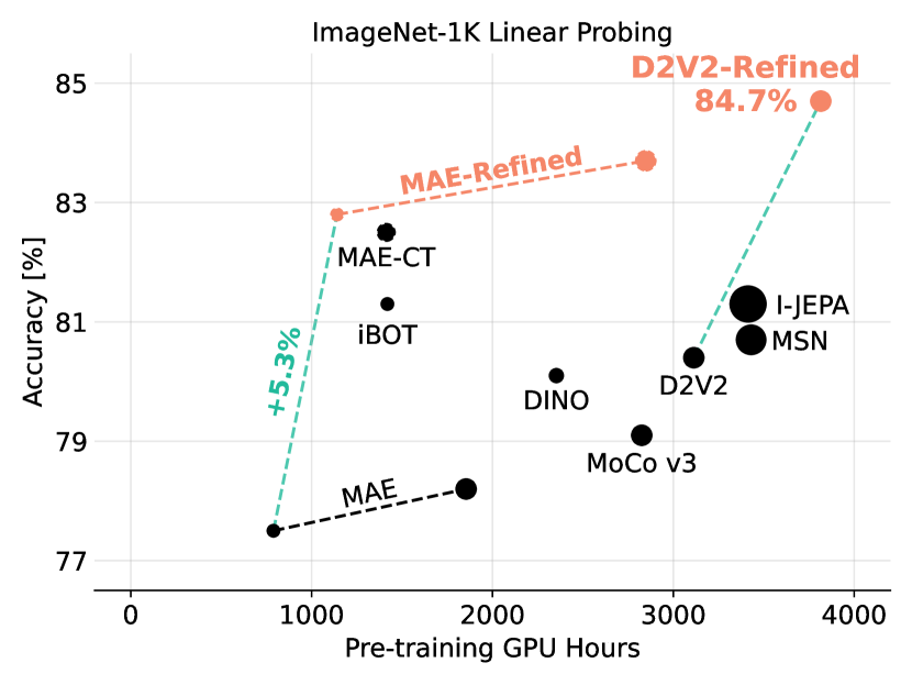
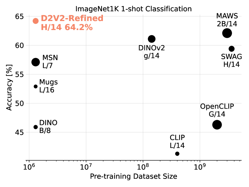
The refinement process is short but effective. Within a few epochs, we refine the features of MIM models from subpar to state-of-the-art, off-the-shelf features. Refining a ViT-H, pre-trained with data2vec 2.0 on ImageNet-1K, sets a new state-of-the-art in linear probing (84.7%) and low-shot classification among models that are pre-trained on ImageNet-1K. At ImageNet-1K 1-shot classification, MIM-Refiner advances the state-of-the-art to 64.2%, outperforming larger models that were trained on up to 2000 times more data such as DINOv2-g, OpenCLIP-G and MAWS-6.5B. Project page: https://ml-jku.github.io/MIM-Refiner

1 Introduction

Figure 1: Linear probing state-of-the-art on ImageNet-1K over the last four years.

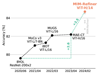
Self-supervised learning (SSL) has attracted considerable attention, owing to its data efficiency and generalization ability [40]. SSL leverages pre-taining tasks and creates intricate input representations without the need for explicit supervision via expensive annotations. In computer vision, Masked Image Modeling (MIM) [11, 59, 49] has emerged as one of the prevalent SSL pre-training paradigms, enabling an efficient pretraining of large models on unlabeled data by reconstructing masked parts of the input images.

The success of MIM is driven by methods like Masked Autoencoder (MAE) [25], data2vec [6, 5], and others [7, 64]. For example, MAE opens the door for sparse pre-training of Vision Transformers (ViTs) [19] by masking large parts of the image and not processing the masked areas. The computational efficiency, coupled with the data efficiency of a generative reconstruction task [65, 22, 55] fosters the scaling to larger architectures on datasets of limited size. However, MIM models tend to spread their attention across the whole image [60]. When adapting to downstream tasks, a sufficient amount of labels is required to rewire the attention to focus on important regions in the image. In the absence thereof, MIM models perform poorly. In contrast, for example, Instance Discrimination (ID) [26, 13, 9, 24] methods implicitly focus on objects and form semantic clusters in the latent space [10], which eases adaption to downstream tasks in the absence of vast amounts of labels. In summary, the most important desiderata for efficient SSL pre-training methods in computer vision are rich representations of the input – ideally in the form of semantic clusters in the latent space – alongside efficiency in both compute and data, and, most notably, favorable scaling to larger architectures.

Figure 2: Left: Representation quality of SSL methods evaluated via linear probing. MIM-Refiner advances state-of-the-art among models pre-trained on ImageNet-1K in low- and high-compute regimes. Right: MIM-Refiner advances state-of-the-art in the extreme setting of 1-shot classification despite being trained on orders of magnitude less data. Size of dots corresponds to model FLOPS.

In this work, we first analyze pre-trained MIM models, where we find that MIM models have different types of blocks: those that mainly improve the pre-training objective and others that are responsible for abstraction within the MIM encoder. The origin of this behavior can be traced back to the fact that MIM architectures usually comprise a large ViT encoder together with a very light-weight decoder. For larger models, the light-weight decoder reaches a point, where it cannot further improve the pre-training objective on its own and passes part of the reconstruction task back to the last encoder blocks. Consequently, the feature quality for downstream tasks of the later blocks degrades, and, somewhat unusual, the representation quality peaks in the middle blocks of the encoder.

Based on these insights, we introduce MIM-Refiner, a sequential refinement approach tailored to MIM models. MIM-Refiner applies an ensemble of ID heads that enforce semantic clusters via an ID objective. Most importantly, those ID heads are attached to intermediate blocks of the encoder including those that exhibit peak representation quality, instead of only a single ID head attached to the last block.

As ID objective, we introduce Nearest Neighbor Alignment (NNA). Given a batch of samples, NNA aligns each sample with its nearest neighbor and repels each sample from all other samples in the batch.

Experimentally, we show that within few epochs, MIM-Refiner refines the features of MIM models from subpar to state-of-the-art, off-the-shelf features, see Figure 2. For example, a refined ViT-H, pre-trained with data2vec 2.0 [5] on ImageNet-1K [17], achieves new state-of-the-art results in linear probing (84.7%, Figure 1), $k$-NN accuracy (82.3%), $k$-means cluster accuracy (67.3%) and low-shot classification among models pre-trained on ImageNet-1K. In ImageNet-1K 1-shot classification it sets a new state-of-the-art of 64.2%, outperforming larger models that were trained on up to 2000x more data such as DINOv2-g, OpenCLIP-G and MAWS-6.5B.

Our contributions can be summarized as follows:

1. We experimentally find that MIM models have different types of blocks: those that mainly improve the pre-training objective and others that are responsible for abstraction within the MIM encoder.

2. We introduce MIM-Refiner, a sequential approach to refine the representation of a pre-trained MIM model to form semantic clusters via an ID objective. Motivated by the findings in (1), MIM-Refiner is designed to exploit the intermediate representations via an ensemble of ID heads attached to multiple encoder blocks.

3. We introduce Nearest Neighbor Alignment (NNA), an ID objective that aligns each sample with its nearest neighbor while repelling other samples in a batch.

2 Challenges of Masked Image Modeling

(a) Encoder-decoder Parameter Count

(b) ImageNet-1K $k$-NN Accuracy per Block

(c) ImageNet-1K Low-shot Accuracy.

(d) Relative Improvements per Block.

Figure 3: (a) MIM models are asymmetrically designed where the encoder has most of the parameters, as indicated by the percentages in the bars. (b) The representation quality of the encoder (measured by $k$-NN accuracy) peaks in the middle blocks before degrading when the later blocks take over parts of the decoder’s task. (c) The decline in representation quality in later blocks primarily contributes to the degradation in downstream performance. ID methods (represented by iBOT [69]) and our MAE-Refined do not suffer from this issue. (d) Correlation of the relative improvement of the reconstruction loss and the relative improvement in the $k$-NN accuracy per block. The relative $k$-NN accuracy improvement is obtained from the $k$-NN accuracy shown in (b). Similarly, the relative improvement of the reconstruction loss is obtained from Figure 7 in the appendix. Middle blocks form abstract representations (large improvements in the $k$-NN accuracy, almost no improvement in reconstruction loss), later blocks take over parts of the reconstruction task (decrease in the $k$-NN accuracy, large improvement in the reconstruction loss). More details in Appendix 0.C.2.

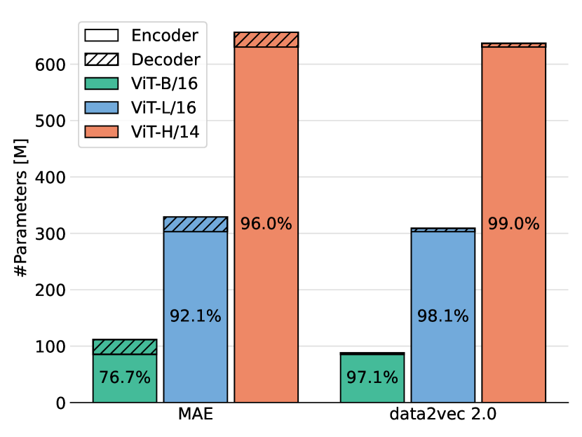
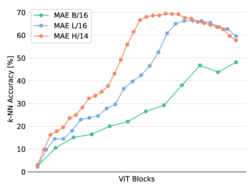
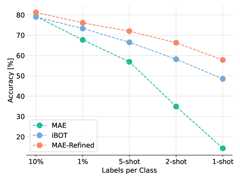
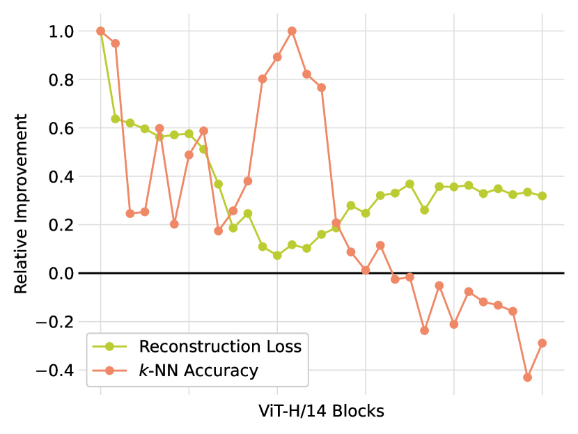
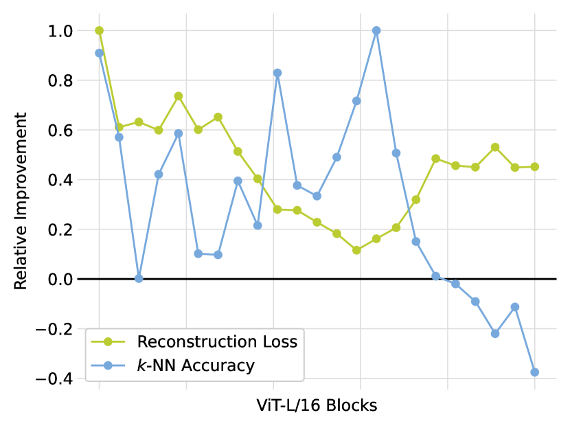
MIM models, such as MAE [25] and data2vec 2.0 [5], enable an efficient pre-training of large models. In terms of architecture, the encoder and decoder are intentionally designed asymmetrically. The encoder, on the one hand, is a large ViT, where discarding 75% of the input patches drastically reduces the cost of a forward pass. The decoder, on the other hand, operates on the full sequence length – by concatenating mask tokens to the encoded visible patches – and, thus, is typically very lightweight to compensate for the increased number of tokens (Figure 3(a)). As models increase in size, the decoder eventually reaches a point where it cannot further improve the pre-training objective on its own. Consequently, it begins to delegate a portion of the reconstruction task back to the last encoder blocks. This transfer adversely affects the feature quality for downstream tasks associated with those blocks (Figure 3(b)), especially when only few labels are available (Figure 3(c)). We observe this phenomenon by correlating the relative improvement in the reconstruction loss vs the $k$-NN accuracy (Figure 3(d)). Roughly speaking, the blocks of the encoder operate in three different regimes:

1. In early ViT blocks, general purpose features are learned, which improve the reconstruction loss and the $k$-NN accuracy simultaneously.

2. In middle ViT blocks, abstractions are formed. The reconstruction loss improves only slightly, while the $k$-NN accuracy improves drastically.

3. In late ViT blocks, features are prepared for the reconstruction task. The reconstruction loss improves at a faster rate, while the $k$-NN accuracy decreases.

When naïvely using the features of the last encoder block, those features are suited for reconstruction, but not particularly for downstream tasks. If lots of labels are available, this can be compensated by fine-tuning the last encoder blocks on the downstream task. However, if not enough labels are available, or the last encoder blocks are not fine-tuned, downstream performance suffers.

3 MIM-Refiner

We propose MIM-Refiner, a novel approach aimed at improving downstream performance by refining the later blocks of a pre-trained MIM model. MIM-Refiner leverages the abstract intermediate representations with an ensemble of Instance Discrimination (ID) heads, which are attached to multiple blocks towards the end of the encoder, as visualized on the left side of Figure 4. The resulting experimental improvements in various downstream tasks are discussed in Section 5.

Figure 4: Left: Comparison of different pre-training schemes. ID uses a single ID head, whereas MIM models use a light-weight decoder to train an encoder. MIM-Refiner attaches multiple ID heads to the later third of the blocks of a pre-trained MIM encoder. Right: Nearest Neighbor Alignment (NNA). An anchor sample is attracted by its NN and simultaneously repelled from other samples in the batch. The NN is retrieved from a first-in-first-out queue of samples from previous batches.

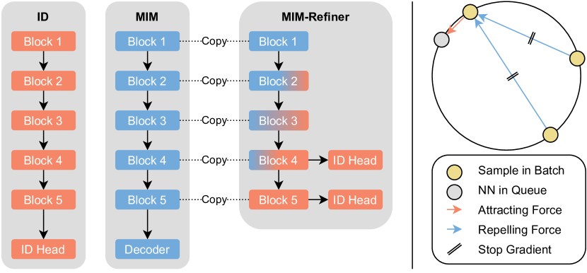
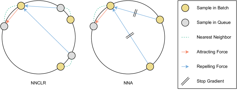
Inspired by NN based contrastive learning [21, 4], we propose Nearest Neighbor Alignment (NNA). NN contrastive objectives introduce an inter-sample correlation by retrieving NNs of samples in a batch and subsequently applying an objective between the samples and their NNs. In practice, the NN retrieval is typically done by tracking samples from previous iterations in a first-in-first-out queue [21, 26]. Therefore, the samples in the queue are from a previous model state which creates a tradeoff between the benefit of the NN-swap and the worse signal from the out-of-sync samples. We argue that the NN-swap does not offer a benefit for negative samples, since there are already different images in every batch, and instead, degrades the signal from the contrastive objective. We therefore propose to use the NN only for the alignment of positive samples, as visualized on the right side of Figure 4. Omitting the NN-swap for the negatives gives a small but consistent improvement as ablated in Table 1. NNA is inspired by NNCLR [21]. Their differences are visualized in Appendix Figure 9.

Formally, given a batch of features $\mathcal{Z}=\{z_{1},\dots,z_{N}\}$ and a queue $\mathcal{Q}$ the NNA objective can be written as:

$$\mathcal{L}^{\text{NNA}}_{i} =-\log\frac{\exp(\text{NN}(z_{i},\mathcal{Q})\cdot z_{i}/\tau)}{\exp(\text{NN}(z_{i},\mathcal{Q})\cdot z_{i}/\tau)+\sum\limits^{N}_{j=1}\exp(\text{SG}(z_{j})\cdot z_{i}/\tau)[i\neq j]}\ ,$$ (1)

$$\text{NN}(z_{i},\mathcal{Q}) =\underset{q\in\mathcal{Q}}{\text{argmax}}(z_{i}\cdot q)\ ,$$ (2)

where $z_{i}$ is the anchor, $\text{NN}(z_{i},\mathcal{Q})$ is the positive, $z_{j}$ are the negatives, $\tau$ is the temperature, and SG is the stop-gradient operation. $[i\neq j]$ denotes the Iverson bracket that evaluates to $1$ if $i\neq j$ and to $0$ if $i=j$. All vectors are assumed to be normalized to length $1$.

4 Related Work

4.1 Pre-training in Computer Vision

Following the success of generative pre-training of transformers [58] in language modeling [18, 52], similar directions were explored in computer vision [19, 64, 61, 12]. With the introduction of Vision Transformers [19], large Masked Image Modeling (MIM) models could be efficiently trained [25, 5, 55] by using the ability of transformers to effortlessly process sparse input by dropping masked patch tokens in the input and subsequently reconstructing the masked parts. In order to optimize the MIM pre-training objective, models have to infer the missing regions by efficiently encoding foreground and background alike which leads to a rich representation.

Building on the rich features learned by MIM models has been explored in various ways. MAWS [55] first pre-trains an MAE, followed by weakly supervised training on a billion-scale dataset and billion-scale models. SemiViT [8] uses a pre-trained MAE as a starting point for semi-supervised learning. Segment Anything [34] use MAE as basis for a segmentation foundation model. MIM-Refiner also builds on the rich features of MIM models and refines them with a ID objective to ease adaption to downstream tasks.

Instance Discrimination (ID) is another branch of self-supervised learning that uses augmentations to create multiple views of the same sample where the task is then to find matching pairs within the views from all samples within a batch [13, 26, 20, 62] or align features of one view with the features from another [24, 10]. We use the terminology that views from the same sample are “positive pairs” and views of different samples are “negative pairs”. When describing a single view of a sample, it is called the “anchor” to which all other views in a batch are either “positives” or “negatives”. NN-based ID [21, 4] extends this setting to use NNs in various ways to create views or otherwise augment samples during training. MIM-Refiner introduces Nearest Neighbor Alignment, which is a modification of previous NN-based ID methods to use the NN only for the alignment part, i.e. pulling the anchor closer to the NN of its positives while pushing the anchor away from its negatives.

4.2 Combining MIM and ID

Adding a MIM to ID methods has emerged as a powerful pre-training scheme. However, in contrast to ID models, the MIM objective in the end-to-end training either uses significantly lower masking ratios with mask tokens getting processed by the encoder [69, 47], or requires a target encoder to encode the unmasked image [29, 2]. Both drastically increase the computational requirements as the encoder operates on the full sequence length. Consequently, these models either require copious amounts of compute to train [47] or limit themselves to relatively small models [69, 29]. Contrary, MIM models have shown success and scalability to large models with comparatively little compute [25, 5, 55]. MIM-Refiner can build on these models which allows us to scale to large model sizes without a large amount of compute. Our largest model, MAE-Refined-2B contains approximately twice the parameters of the currently largest uni-modal contrastive model DINOv2-g [47] and can be trained on two orders of magnitude less data.

Attempts to preserve the efficiency while training MIM and ID objectives end-to-end have been less successful [38, 32], where both works came to the conclusion that sequential training (MIM $\rightarrow$ ID) circumvents various problem with end-to-end training. First, a powerful encoder is trained solely with a MIM objective. Second, the encoder is trained with a ID objective while preserving the rich features in early blocks with a layer-wise learning rate decay [15] in lower blocks and either constraining changes in early blocks [32] or completely freezing them [38].

MIM-Refiner is also a sequential MIM $\rightarrow$ ID method. In contrast to our work, previous works start from the representation after the last MIM encoder block and are therefore highly reliant on a good representation thereof. This can be seen for example on MAE-CT [38] where their ViT-H/14 model is worse than their ViT-H/16 model, despite using 30% more FLOPS. On the current landscape of MIM models, this limits their method to MAE [25], since other MIM models have a far worse representation in the last block after pre-training (e.g. MAE has 58.1% $k$-NN accuracy while data2vec 2.0 has only 48%). Additionally, previous works [38, 32] omit current go-to techniques such as multi-crop augmentation [9] which has been shown to improve performance [10, 70, 69].

Training models with additional losses from intermediate layers dates back to the early deep learning days [37, 56] where these auxiliary losses were used to alleviate optimization issues in lower layers. MIM-Refiner relates to deep supervision in the sense that we use multiple ID heads attached at intermediate layers where each head produces a loss for training.

5 Experiments

We focus our work on two prominent MIM models that are publicly available, namely MAE [25, 55] and data2vec 2.0 [5] (abbreviated as D2V2). These models were pre-trained on ImageNet-1K, which we also use for the refinement.

We first discuss and ablate different design choices of MIM-Refiner. We then evaluate our models in various settings including low-shot classification, feature evaluation, clustering, transfer learning and semantic segmentation.

5.1 Ablation Study

We investigate various design choices of our method in Table 1.

(a) Adding multiple heads at intermediate features improves $k$-NN accuracy by 0.8%. The best settings include the blocks with the best representation quality (see Figure 3(b)). Adding additional heads before the best blocks does not improve performance while increasing training costs.

(b) Spacing heads out across the last third of the encoder blocks achieves comparable results to simply using eight heads while requiring less compute. We find the default setting of attaching ID heads to the last third of the blocks to work well across MIM methods and model sizes whereas using less heads with larger spacing between them would require a more careful selection depending on the model and its size (see Appendix Table 6).

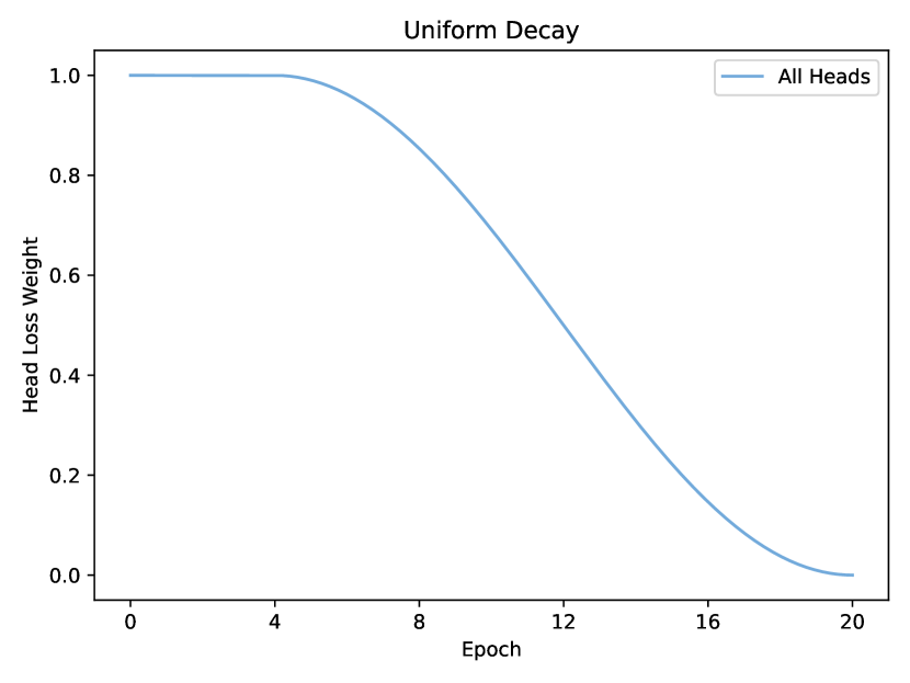
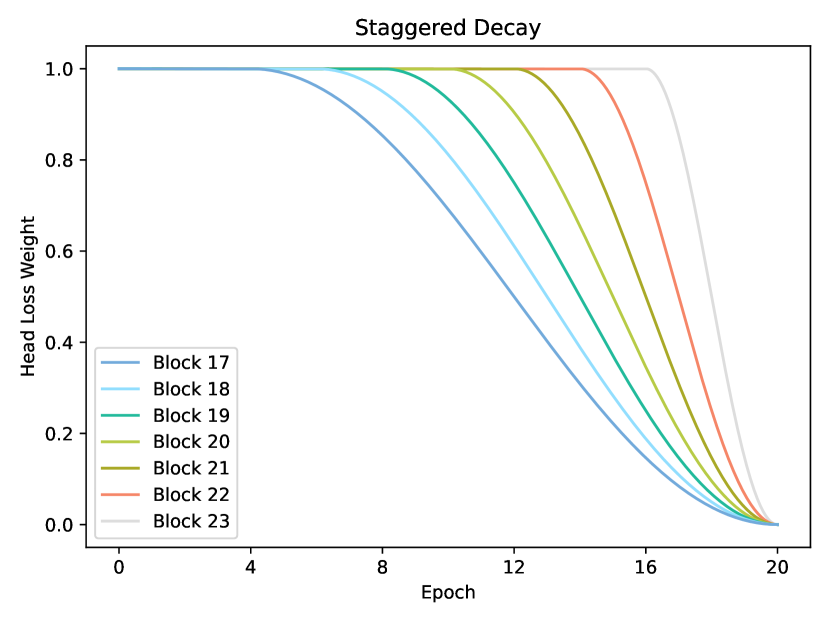
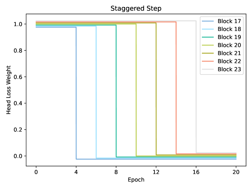
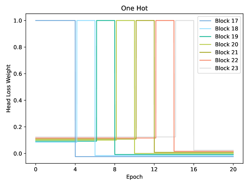
(c) Scheduling the loss weight of each intermediate head is not necessary, i.e., simply summing all losses is sufficient to achieve good performances. “Uniform Decay” decays the loss weight of all intermediate heads during training. “Staggered Decay” starts by decaying the first head and gradually starts to decay more and more heads as training progresses. “Staggered Step” disables the first head after some time followed by gradually disabling more and more heads. “One Hot” trains the encoder with only one intermediate head at a time where training starts with the earliest intermediate head and gradually iterates through the heads. Details to the loss schedules are in Appendix 0.C.11.

(d) Freezing early blocks as a form of regularization to preserve MIM features (similar to related works [38, 32]) is not necessary for MIM-Refiner. Note that we still use a layer-wise learning rate decay [15].

(e) Using the NN swap only for aligning the positive with the anchor is slightly better than also swapping the negatives with their NN.

(f) Multi-crop augmentation [9] greatly improves performance. Relying only on the data-driven augmentation of the NN-swap [21] by omitting color/blur augmentations, is beneficial for certain downstream tasks such as low-shot classification [38]. We further investigate training without color/blur augmentations on a ViT-H/14 in Appendix 0.A.2 which also improves performance in low-shot classification.

#Heads	$k$-NN
1	80.2
2	80.2
4	80.9
8	81.0
12	81.0

(a)

Block Indices	$k$-NN
20, 24	80.9
16, 20, 24	81.1
15, 18, 21, 24	81.1
18, 20, 22, 24	81.0
17-24	81.0

(b)

Schedule	$k$-NN
Constant	81.0
Uniform Decay	80.9
Staggered Decay	81.0
Staggered Step	80.9
One Hot	80.7

(c)

#Frozen	$k$-NN
0	81.0
6	80.9
12	80.6

(d)

Swap Neg.	$k$-NN
✗	81.0
✓	80.9

(e)

Color/Blur	Multi-crop	$k$-NN	1-shot
✓	✗	78.4	58.9
✓	✓	81.0	61.7
✗	✓	80.5	63.4

(f)

Table 1: Ablation study by refining data2vec 2.0 ViT-L/16. Default settings

5.2 ImageNet-1K Low-shot and Frozen Feature Evaluations

We evaluate the ability of our models to perform low-shot classification in Table 2. Additionally, linear probing and $k$-NN accuracy are reported which are computed from the features of the frozen encoder. These metrics are typically correlated to low-shot performance as it indicates that the representation is already linear separable which eases drawing decision boundaries given only few labels. Note that we use the linear probing protocol of DINOv2 [47] which includes using features of the last four blocks in its hyperparameter grid. Therefore, linear probing evaluates the feature representation at the end of the encoder, while $k$-NN accuracy evaluates only the features of the last block.

MIM-Refiner significantly improves upon MIM models and other SSL models. In the 1-shot settings D2V2-Refined H/14 sets a new state-of-the-art of 64.7%, outperforming the 63.6% of MAWS ViT-6.5B/14 [55] which is pre-trained on a private dataset with approximately 2000 times the size of ImageNet-1K.

ViT	Method	Low-shot Evaluation					Feature Eval
		1-shot	2-shot	5-shot	1%	10%	Probe	$k$-NN
L/16	MAE [25]	14.3	34.9	56.9	67.7	79.3	77.5	60.6
	data2vec 2.0 [5]	24.1	58.8	72.1	75.1	81.5	78.2	51.8
	iBOT [69]	48.5	58.2	66.5	73.3	79.0	81.1	78.0
	Mugs [70]	52.9	62.3	69.4	76.2	80.3	82.1	80.4
	MAE-Refined	57.8	66.3	72.0	76.1	81.2	82.8	81.5
	D2V2-Refined	61.7	69.6	73.9	78.1	82.1	83.5	81.0
H/14	MAE [25]	7.2	14.1	40.2	72.8	81.2	78.2	58.1
	data2vec 2.0 [5]	21.6	60.8	74.2	77.6	83.3	80.4	48.0
	I-JEPA [3]	35.1	47.9	59.9	73.3	79.5	79.3	71.6
	MAE-CT [38]	49.4	59.6	67.4	74.4	81.7	82.3	79.1
	MAE-Refined	59.5	68.5	73.8	77.4	82.1	83.7	82.3
	D2V2-Refined	64.2	71.3	75.5	78.1	83.5	84.7	82.3
2B/14	MAE [25, 55]	17.8	29.1	62.9	73.6	82.0	79.7	67.1
	MAE-Refined	58.2	68.6	74.8	78.7	82.5	84.5	83.2
L/7	MSN [2] (IN-1K)	57.1	66.4	72.1	75.1	-	80.7	-
L/16	iBOT [69] (IN-22K)	37.4	49.9	61.9	70.9	80.3	82.7	72.9
g/14	DINOv2 [47] (LVD-142M)	60.5	68.3	74.4	79.1	83.8	86.5	83.5
H/14	D2V2-Refined (IN-1K)	64.2	71.3	75.5	78.1	83.5	84.7	82.3

Table 2: Low-shot and feature evaluations of recent SSL models on ImageNet-1K. MIM-Refiner significantly improves in-class state-of-the-art and also compares favorably against some larger models and/or larger pre-training datasets. Our Models

5.3 ImageNet-1K Cluster Evaluations

ViT	Method	Cluster Performance				Class Separation
		ACC	NMI	AMI	ARI	SIL ($\uparrow$)	DBS ($\downarrow$)
L/16	MAE [25]	18.5	55.2	29.1	6.9	-5.9	5.0
	data2vec 2.0 [5]	10.5	45.1	19.5	2.5	-9.1	6.4
	iBOT [69]	52.2	80.5	67.0	33.4	13.3	3.5
	Mugs [70]	54.3	78.6	65.5	22.4	14.9	3.3
	MAE-Refined	61.8	84.0	72.6	40.7	21.4	2.9
	D2V2-Refined	67.4	86.3	76.2	40.5	37.1	2.2
H/14	MAE [25]	14.3	50.2	24.2	4.3	-7.8	5.2
	data2vec 2.0 [5]	9.9	45.8	18.0	2.6	-10.8	6.5
	MAE-Refined	64.6	85.3	74.6	45.5	21.0	2.9
	D2V2-Refined	67.3	87.2	77.9	42.2	34.5	2.3
2B/14	MAE [25, 55]	19.9	54.1	33.1	6.2	-3.6	4.8
	MAE-Refined	63.0	85.0	74.4	44.0	14.0	3.2
g/14	DINOv2 [47] (LVD-142M)	47.7	76.3	63.6	5.1	30.4	2.8
H/14	D2V2-Refined (IN-1K)	67.3	87.2	77.9	42.2	34.5	2.3

Table 3: $k$-means cluster performance and class separation on ImageNet of recent SSL models. MIM-Refiner drastically improves performance of unrefined models and outperforms competitors. Our Models

We compare the cluster performance of MIM and MIM-Refined models against recent SSL models in Table 3. For this experiment, we apply mini-batch $k$-means [54] to the validation set of ImageNet-1K. We perform mini-batch $k$-means 100 times on each embedding and select the run with lowest $k$-means loss for comparison (average performance is reported in Appendix Table 9). We report commonly used metrics for measuring Cluster Performance w.r.t. the ground truth clustering: Cluster Accuracy (ACC) [66], Normalized Mutual Information (NMI) [36], Adjusted Mutual Information (AMI) [45], Adjusted Rand Index (ARI) [30], where higher values indicate a better match of the found clustering with the ground truth labels. Further, we measure the Class Separation in the embedded space using the Davies-Bouldin score (DBS) [16] and silhouette score (SIL) [53] w.r.t. the ground truth classes. The DBS measures the separation and compactness of classes, where lower values are better and zero is the minimum. The SIL ranges from -100 to 100, where higher values are better. Negative SILs relate to mismatches between classes and embedding, where scores close to zero indicate a potential overlap of classes.

Table 3 shows that ACC is increasing more than threefold from MAE/D2V2 (18.5/10.5) to their refined counterparts MAE-Refined/D2V2-Refined (61.8/67.4) for ViT L/16. This holds true for other model sizes as well. The reached ACC of 67.4 outperforms the current state-of-the-art of 61.6 reached by TEMI MSN [1]. The improvement in cluster performance shows in the enhanced separation of classes in the embedding as well. MIM-Refiner lifts MAE and D2V2 from negative SILs to positive double digit scores, indicating the formation of clearer semantic clusters after refinement. The DBS shows this improvement as well, by about a factor of two reduction after refinement. Figure 6 illustrate this drastic increase in cluster performance and class separation visually.

\begin{overpic}[width=433.62pt]{res/d2v2-large16_ccwnwqmn_plot_food_large16.pdf} \scriptsize \put(20.0,-5.0){ACC: 19.3 $|$ SIL: -12.2} \end{overpic}

(a) D2V2

\begin{overpic}[width=433.62pt]{res/d2v2-large16-refined-5yvj2un6_f3slqv9a_plot_food_large16.pdf} \scriptsize \put(19.0,-5.0){ACC: 70.3 $|$ SIL: 32.4} \end{overpic}

(b) D2V2-Refined

\begin{overpic}[width=433.62pt]{res/mugs_large16_067cpxym_plot_food_large16.pdf} \scriptsize \put(20.0,-5.0){ACC: 64.3 $|$ SIL: 10.0} \end{overpic}

(c) Mugs

Figure 6: UMAP [43] plots of embeddings from D2V2, D2V2-Refined and Mugs for ViT-L on all food related classes of ImageNet. The corresponding $k$-means cluster accuracy (ACC) and class separation measured in silhouette score (SIL) is shown below each plot. Clusters in D2V2 (a) are visually more condensed and better separated with corresponding improvements in ACC and SIL after refinement (b). Mugs (c) does not separate the clusters that well, as shown by the merged clusters in the middle and the lower SIL score. The colors show the 53 ground truth food classes.

5.4 Experiments on other Datasets

We investigate generalization of MIM-Refiner to other datasets with low-shot fine-tuning on iNaturalist18 [28] and linear probing to a diverse set of datasets. For linear probing, we evaluate classification on iNaturalist18 [28], generalization to a diverse set of seven classification tasks from VTAB [67] and semantic segmentation on ADE20K [68]. From VTAB, we use the seven datasets from the “Natural” category which consists of Caltech101 [23], CIFAR-100 [35], DTD [14], Flowers102 [46], Pets [48], Sun397 [63] and SVHN [44]. Due to the prohibitively large costs of fine-tuning large ViT models on a semantic segmentation task, we instead opt for a protocol similar to DINOv2 [47]. We train a linear probe that assigns a class to each patch and upscale the predictions to the input resolution.

Table 4 shows the benefits of MIM-Refiner models when transferring a pre-trained representation to various datasets. MAE-Refined consistently improves over MAE and shows overall strong performances and favorable scaling to larger models. D2V2-Refined improves over D2V2 on iNaturalist classification but does not improveme on VTAB and ADE20K. Since we use close to identical settings for refining MAE and D2V2 (see Appendix Table 10), we hypothesize that inherent differences within the pre-trained representation exist, which influence generalization capabilities. While D2V2 [5] demonstrates that their pre-training can also be applied to speech processing and natural language processing, generalization beyond ImageNet was not thoroughly explored for their vision models.

		iNat18 fine-tuning			Linear Probe
Method	Arch.	1-shot	5-shot	10-shot	iNat18 ($\uparrow$)	VTAB ($\downarrow$)	ADE20K ($\uparrow$)
MAE [25]	L/16	7.1	51.6	68.9	42.8	10.0	58.5
D2V2 [5]	L/16	5.5	53.1	70.6	39.4	9.5	60.9
DINO [10]	B/8	19.8	55.1	69.3	59.7	6.8	59.4
iBOT [69]	L/16	15.8	51.5	65.5	56.0	6.4	58.4
Mugs [70]	L/16	19.5	53.2	66.9	61.5	6.6	61.5
MAE-Refined	L/16	19.0	58.0	71.7	60.6	5.0	59.4
D2V2-Refined	L/16	15.2	56.3	71.8	52.0	9.9	60.3
MAE [25]	H/14	6.5	53.3	71.7	43.0	10.8	59.7
D2V2 [5]	H/14	5.9	55.7	73.4	41.7	7.4	62.5
MSN [2]	L/7	17.0	38.0	74.4	-	-	-
MAE-Refined	H/14	20.9	62.4	75.4	64.6	3.6	60.8
D2V2-Refined	H/14	16.1	59.2	74.8	54.4	7.4	62.2
MAE [25, 55]	2B/14	10.0	53.7	72.2	51.0	6.4	61.0
MAE-Refined	2B/14	22.5	63.5	76.5	69.6	1.4	61.6

Table 4: Transferring MIM-Refiner models to other datasets. VTAB reports the average rank among seven datasets from the VTAB benchmark [67], detailed results are shown in Appendix Table 8. ADE20K reports the mean intersection over union (mIoU) of a semantic segmentation head. MIM-Refiner, especially MAE-Refined, learns general features that can easily be transferred to other datasets and tasks.

5.5 Fine-tuning with Large Amounts of Labels

We investigate if our refining procedure involuntarily degrades the performance when an abundance of labels is available. To this end, we fine-tune MAE models and their refined version on ImageNet-1K [17] and iNaturalist18 [28]. Table 5 shows that the refined models perform slightly better with 100% of the labels.

Model	ViT-L/16		ViT-H/14
	ImageNet-1K	iNat18	ImageNet-1K	iNat18
MAE	85.7	80.7	86.7	82.7
MAE-Refined	85.6	80.9	86.9	83.3

Table 5: Full fine-tuning using 100% of the labels.

6 Limitations

One limitation of MIM-Refiner is that it requires batch normalization [31] layers in the ID head. Without them, performance decreases significantly. As we do not change anything in the MIM pre-training, we hypothesize that feature statistics after MIM pre-training are not suited for an ID task and therefore require per-feature normalization. The batch normalization layers significantly decrease scalability to distributed hardware setups as each batch normalization layer requires a synchronization of batch statistics. This limitation can possibly be alleviated by normalizing with feature statistics from previous iterations (akin to the centering operation in self-distillation ID methods [10]), which can be communicated asynchronously.

MIM-Refiner addresses a common issue with MIM models: their typically lightweight decoder often delegates part of the reconstruction to the encoder, resulting in subpar representations for the later encoder blocks in downstream tasks. Alternatively, one could simply argue for a larger decoder. However, a larger decoder drastically increases computational costs since the decoder operates on the full sequence length. The direction of a larger decoder was explored to a certain extent in the original MAE paper [25], where larger decoders performed worse in fine-tuning and linear probing.

7 Conclusion

We introduce MIM-Refiner, a procedure to refine pre-trained MIM models. Motivated by the insights that the representation quality of MIM models peaks in the middle of the encoder, we employ an ensemble of contrastive heads attached at multiple blocks towards the end of the encoder, including the blocks where representation quality peaks, to improve upon the best existing representation. We train this ensemble for a short duration to improve the representation for downstream tasks. As contrastive objective we introduce Nearest Neighbor Alignment, an adaption of existing nearest neighbor based objectives that uses the nearest neighbor relation to align positive pairs and not to push negative pairs apart, which improves the signal quality from the negatives.

Our refined MIM models learn strong features from ImageNet-1K alone that can be readily used for downstream tasks such as classification or clustering. Our models outperform competitors that were also trained on ImageNet-1K and sometimes also ones that were trained on more data or use larger models.

8 Acknowledgements

We thank Johannes Lehner for helpful discussions and suggestions.

We acknowledge EuroHPC Joint Undertaking for awarding us access to Karolina at IT4Innovations, Czech Republic and Leonardo at CINECA, Italy.

The ELLIS Unit Linz, the LIT AI Lab, the Institute for Machine Learning, are supported by the Federal State Upper Austria. We thank the projects Medical Cognitive Computing Center (MC3), INCONTROL-RL (FFG-881064), PRIMAL (FFG-873979), S3AI (FFG-872172), EPILEPSIA (FFG-892171), AIRI FG 9-N (FWF-36284, FWF-36235), AI4GreenHeatingGrids (FFG- 899943), INTEGRATE (FFG-892418), ELISE (H2020-ICT-2019-3 ID: 951847), Stars4Waters (HORIZON-CL6-2021-CLIMATE-01-01). We thank Audi.JKU Deep Learning Center, TGW LOGISTICS GROUP GMBH, Silicon Austria Labs (SAL), FILL Gesellschaft mbH, Anyline GmbH, Google, ZF Friedrichshafen AG, Robert Bosch GmbH, UCB Biopharma SRL, Merck Healthcare KGaA, Verbund AG, GLS (Univ. Waterloo), Software Competence Center Hagenberg GmbH, Borealis AG, TÜV Austria, Frauscher Sensonic, TRUMPF and the NVIDIA Corporation.

Appendix 0.A Extended Results

0.A.1 Where to Attach ID Heads?

Table 1 ablates different choices of where to attach ID heads on a data2vec 2.0 pre-trained ViT-L/16 and ViT-H/14. On ViT-L/16, there is almost no difference of where to attach the ID heads in the last third of blocks. We tried to transfer this insight to ViT-H/14 where the default setting of attaching ID heads to all later layers performs better. We therefore use the default setting of attaching ID heads to the last 8 blocks (ViT-L/2B) or the last 12 blocks (ViT-H).

Block Indices	$k$-NN
20,24	80.9
16,20,24	81.1
15,18,21,24	81.1
18,20,22,24	81.0
17-24	81.0

(a) ViT-L/16

Block Indices	$k$-NN
22,24,26,28,30,32	82.0
16,18,20,22,24,26,28,30,32	82.1
20-32	82.3

(b) ViT-H/14

Table 6: Spacing heads out more across the later ViT blocks can achieve comparable performances for ViT-L/16 but does not generalize to ViT-H/14. The default setting of attaching ID heads to all later blocks generalizes well across model scales.

0.A.2 Low-shot Classification without Color Augmentations

MAE-CT [38] showed that omitting color augmentations can lead to performance gains for low-shot classification, especially on larger models. We therefore train our ViT-H/14 models also without color augmentations. We use the same hyperparameters as with color augmentations (see Table 10) except that we disable color augmentations (i.e. we train with only crop & flip augmentations) and half the training duration.

Model	Color	Low-shot Evaluation					Feature Eval
	Augmentations	1-shot	2-shot	5-shot	1%	10%	Probe	$k$-NN
D2V2-Refined	✗	64.7	72.0	75.9	79.1	83.5	84.1	82.1
D2V2-Refined	✓	64.2	71.3	75.5	78.1	83.5	84.7	82.3

Table 7: ImageNet-1K low-shot and feature evaluations of a refined data2vec 2.0 ViT-H/14 with and without color augmentations. Omitting color augmentations (i.e. using only crop & flip augmentations) improves ImageNet-1K low-shot performance.

0.A.3 VTAB Results

We show detailed results for the seven considered datasets from the VTAB benchmark [67] in Table 8. As the benchmark consists of a broad variety of images, we rank the performance of all models per dataset and report the average rank.

Method	Arch.	CT101	CF-100	DTD	FL102	Pets	Sun397	SVHN	Rank
MAE	L/16	91.0	79.6	78.0	91.6	91.9	76.0	75.7	10.0
D2V2	L/16	90.7	85.0	76.4	92.6	86.7	76.8	77.5	9.5
DINO	B/8	90.5	86.6	80.4	97.8	93.4	77.4	74.6	6.8
iBOT	L/16	90.9	89.2	79.6	97.3	93.7	77.7	69.9	6.4
MUGS	L/16	89.6	89.4	78.4	97.8	95.4	77.2	76.5	6.6
MAE-Refined	L/16	91.1	89.0	80.4	97.1	96.0	79.0	71.1	5.0
D2V2-Refined	L/16	88.7	88.8	75.6	94.1	94.7	77.3	59.1	9.9
MAE	H/14	89.8	81.1	78.3	91.5	91.6	76.3	73.0	10.8
D2V2	H/14	90.5	87.0	80.0	92.9	86.2	78.3	77.8	7.4
MAE-Refined	H/14	91.2	90.0	82.0	98.0	96.1	79.5	69.7	3.6
D2V2-Refined	H/14	89.2	90.5	77.4	95.3	95.7	78.4	61.7	7.4
MAE	2B/14	91.5	82.5	79.5	93.5	92.8	77.9	78.5	6.4
MAE-Refined	2B/14	91.8	90.8	82.8	98.2	96.5	80.3	77.5	1.4

Table 8: Linear probing accuracy on the seven VTAB [67] datasets from the “Natural” category: Caltech101 [23], CIFAR-100 [35], DTD [14], Flowers102 [46], Pets [48], Sun397 [63] and SVHN [44].

0.A.4 Extended ImageNet-1K Cluster Evaluations

Table 9 shows the average clustering results of the 100 mini-batch $k$-means runs as described in Section 5.3. We see that MIM-Refiner has also better average performance than competitor methods.

ViT	Method	Cluster Performance
		ACC	NMI	AMI	ARI
L/16	MAE [25]	17.9	54.5	28.9	6.5
	data2vec 2.0 [5]	10.2	44.5	19.3	2.3
	iBOT [69]	50.5	80.0	66.6	31.6
	Mugs [70]	50.7	77.4	64.4	18.1
	MAE-Refined	60.6	83.5	71.9	35.0
	D2V2-Refined	60.6	83.9	72.9	30.0
H/14	MAE [25]	13.8	49.8	24.4	4.2
	data2vec 2.0 [5]	9.7	45.2	18.1	2.5
	MAE-Refined	63.2	84.7	74.0	40.1
	D2V2-Refined	60.4	84.5	74.3	28.4
2B/14	MAE [25, 55]	19.2	53.5	32.9	5.7
	MAE-Refined	59.4	84.0	73.4	38.0
g/14	DINOv2 [47] (LVD-142M)	46.8	75.6	62.7	3.5
H/14	D2V2-Refined (IN-1K)	60.4	84.5	74.3	28.4

Table 9: Average $k$-means cluster performance on ImageNet of recent SSL models. MIM-Refiner drastically improves performance of unrefined models and outperforms competitors. For each model size the best model is bold and second best is underlined.

Appendix 0.B Implementation Details

0.B.1 Vision Transformer

The architecture of our models follows the ones from the respective MIM model that is refined. That is a pre-norm architecture for MAE [25] and a post-norm architecture for data2vec 2.0 [5]. We attach the ID heads to the [CLS] tokens and also use the [CLS] token for evaluation.

0.B.2 ID Head Architecture

We use a three layer MLP with hidden dimension 2048 as projector and a two layer MLP with hidden dimension 4096 as predictor. Each linear projection is followed by a GELU [27] and a batchnorm [31] layer. For the last linear projection in projector and predictor, no GELU is used.

0.B.3 Refinement Hyperparameters

Hyperparameters for the refinement stage are listed in Table 10. Following MAE-CT [38], we initialize all ID heads first by training them with a frozen encoder to ensure a good learning signal from the start of the refinement process. We use the same hyperparameters except that we use 20 epochs for all models, a learning rate of $2e-4$ and a top1-NN lookup. As we do not use a momentum encoder during training, we instead track an EMA of the encoder and use the EMA then for downstream tasks. As ViT-2B is very expensive to train, we freeze the first 6 layers (for refinement and also for evaluation). As shown in Table 1 this slightly reduces performance but also reduces memory consumption and runtime.

Parameter	Value
Epochs	30 (MAE L/H), 20 (MAE 2B, data2vec 2.0)
Batch Size	1024 (L), 512 (H, 2B)
Optimizer	AdamW [33, 41]
Momentum	$\beta_{1}=0.9,\beta_{2}=0.95$
Learning Rate Schedule	Linear Warmup $\rightarrow$ Cosine Decay
Warmup Epochs	4
Learning Rate	4e-4
Encoder
Layer-wise LR Decay [15]	0.65
Freeze Layers	0 (everything exept ViT-2B), 6 (ViT-2B)
Weight Decay	0.05
EMA [51]	0.9999
NNCLR Heads
Weight Decay	1e-5
Temperature	0.2 (L), 0.3 (H), 0.35 (2B)
topk-NN $k$	20
NN-swap for Positives	✓
NN-swap for Negatives	✗
Data Augmentation
Color & Blur Settings	see BYOL [24]
Global Views	2
Global View Resolution	224
Global View Scale	[0.25, 1.0]
Local Views	10
Local View Resolution	96 (L), 98 (H)
Local View Scale	[0.05, 0.25]

Table 10: MIM-Refiner hyperparameters.

Appendix 0.C Evaluation Details

0.C.1 GPU Hours Benchmark

For benchmarking GPU hours, we follow the setup from MAE-CT [38]: we conduct a comparison by implementing all methods in a single code-base and conducting short training runs on a single A100 40GB PCIe card. These runs are executed in mixed precision training mode and with the highest possible batchsize that is a power of 2. The runtime of these benchmark runs is then extrapolated to the reported number of epochs. Benchmarks are conducted in pytorch 2.1 with CUDA 12.1. FLOPS are measured with the fvcore library. For the 1-shot classification plot in Figure 2, we do not take into account that some models train on higher resolutions (e.g. DINOv2) for visual clarity.

0.C.2 MAE Intermediate Representation Analysis

We analyze how well the features of a ViT block are suited for reconstruction by training an MAE with a decoder attached after every ViT block. We use the same parameters as for training from scratch [25] but reduce training duration to 20 epochs, warmup to 5 epochs and the depth of all decoders to 2. The encoder remains fully frozen during training and only the decoders are trained.

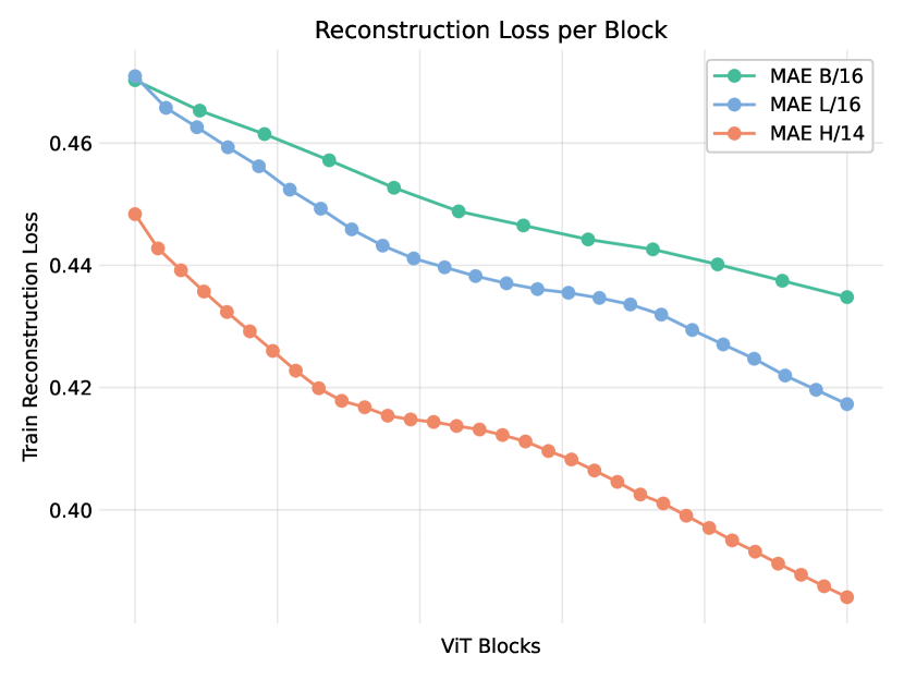
For the visualization in Figure 3(d), we calculate the delta from one block to the next and normalize the deltas by dividing by the maximum delta. We do this for both the $k$-NN accuracy and the reconstruction loss. Figure 7 shows the reconstruction loss per block and the same plot for a MAE L/16, where a similar behavior can be observed.

Figure 7: Left: Reconstruction loss per block of MAEs. Right Relative improvement of reconstruction loss and $k$-NN accuracy for a MAE L/16.

0.C.3 ImageNet-1K Linear Probing Evaluation Details

For linear probing, we use the protocol from DINOv2 [47] for publicly released models and the values from the original papers otherwise. We train for 50 epochs using SGD with momentum 0.9. As data augmentation we use $\tt{RandomResizedCrop}$ and $\tt{HorizontalFlip}$. The DINOv2 protocol sweeps over the following hyperparameters by training multiple linear classifiers at once:

• 13 learning rates ranging from 0.0001 to 0.5

• Use the last layer output or concatenate the output of the last 4 layers

• Use the [CLS] token or the concatenation of [CLS] and [AVG] token

As the linear probes trained on the concatenation of the last 4 layers have more features and more parameters to discriminate between classes, they tend to be the best within the sweeped parameters. Note that we evaluate the representation of the last layer in isolation via $k$-NN classification. We investigate $k$-NN classification with features from the last 4 layers in Appendix 0.C.10.

0.C.4 ImageNet-1K $k$-NN Classification Details

For $k$-NN classification, we follow the protocol of DINO [62, 10]. We train a soft $k$-NN classifier weighted by cosine similarity with $k=10$. For MIM models, higher values for $k$ are beneficial, so we tune this parameter for MAE and data2vec 2.0.

0.C.5 ImageNet-1K Low-shot Evaluation Details

For the 1, 2 and 5-shot benchmarks we train a logistic regression [10, 2] using the [CLS] token after the last encoder block with the cyanure [42] library. As MIM models benefit from fine-tuning in this setting [2], MAE and data2vec 2.0 are fine-tuned instead. We report the average of three dataset splits from MSN [2].

In the 1% and 10% low-shot benchmark, all models are fine-tuned with hyperparameters similar to those used in related works [38, 3, 8]. As the parameters vary between 1%/10% and also between model sizes, we refer to the codebase for the exact protocols.

For a fair comparison, we conduct the low-shot evaluations of DINOv2 at 224 resolution. We study the impact of the higher resolution where we observe minimal gains at the original resolution (518x518). Note that DINOv2 first trains at 224x224 followed by a short training at 518x518 resolution.

resolution	#patches	FLOPS [G]	1-shot	2-shot	5-shot
224x224	256	291	60.5	68.3	74.4
518x518	1369	1553	61.1	68.8	74.8

Table 11: ImageNet-1K low-shot evaluation of DINOv2 g/14 on higher resolutions.

0.C.6 iNat18 Transfer Learning Evaluation Details

We report the accuracy on the validation set averaged over three seeds.

For 1-shot classification on iNat18, we use the linear probing protocol from DINOv2 [47]. We also attempted to fine-tune MIM models where some models fail to exceed random performance and therefore also use linear probing.

For 5-shot and 10-shot classification on iNat18, we fine-tune all models. The hyperparameters for fine-tuning (Table 12) are inspired by MAWS [55].

Parameter	Value
Epochs	50
Batch size	256
Optimizer	AdamW [41, 33]
Learning rate	1e-3
Layer-wise lr decay [15]	0.75
Weight decay	0.05
Momentum	$\beta_{1}=0.9,\beta_{2}=0.999$
Learning rate schedule	linear warmup $\rightarrow$ cosine decay
Warmup epochs	5
Label smoothing [57]	0.1
Data Augmentation
Resize	256
interpolation	bicubic
RandomResizedCrop	224
scale	[0.08, 1.0]
interpolation	bicubic
RandomHorizontalFlip	$p=0.5$

Table 12: Hyperparameters for fine-tuning on iNat18 low-shot classification.

0.C.7 ADE20K Semantic Segmentation

State-of-the-art models in semantic segmentations are prohibitively expensive to train. Therefore, we opt for a simple light-weight evaluation protocol to compare our models on a segmentation task:

• We keep resolution at 224x224

• We freeze the encoder

• We train a linear classifier similar to DINOv2 [47] that predicts a class for each patch. The resulting low-resolution prediction is then upsampled to 224x224 resolution.

• For evaluation, we do not use any advanced methods like multi-scale or multi-crop evaluation but instead opt for a simple protocol of rescaling the shortest edge to 224 followed by a center crop.

As intermediate representations are commonly used for semantic segmentation, we use features from the last block, the 5th last block, the 9th last block and the 13th last block. Compared to simply using the last 4 blocks, this improves performance for all compared models.

0.C.8 Transfer Learning Linear Probing

For transfering the pre-trained features to other datasets (Table 4) we use the DINOv2 [47] linear probing protocol as described in Appendix 0.C.3. For ADE20K and iNat18, we reduce the hyperparameter grid to fit into 40GB GPU memory.

0.C.9 Fine-tuning with 100% Labels

For fine-tuning with 100% of the labels (Table 5), we use the hyperparameters provided in MAE [25] for both iNat18 and ImageNet-1K.

0.C.10 High-dimensional $k$-NN

The linear probing protocol of DINOv2 [47] includes the possibility to concatenate features of the last 4 blocks as input to the linear probe. We find that this outperforms using only the features of the last block in most cases. As the best linear probe uses features from the last 4 blocks and the fact that the $k$-NN and linear probing metrics are typically correlated [47], we report the $k$-NN accuracy using only the features of the last block in Table 2 to use the last 4 blocks for one metric and only the last block for the other. In Table 13 we investigate using the concatenation of features from the last 4 blocks for a $k$-NN classifier. Most models benefit from using more features, especially MIM models.

Method	Arch.	#Blocks		Delta
		1	4
MAE	L/16	60.6	63.3	+2.7
data2vec 2.0	L/16	51.8	52.9	+1.1
iBOT	L/16	78.0	78.9	+0.9
MUGS	L/16	80.4	80.1	$-$0.3
MAE-Refined	L/16	81.5	81.5	+0.0
D2V2-Refined	L/16	81.0	81.7	+0.7
MAE	H/14	58.1	61.4	+3.3
data2vec 2.0	H/14	48.0	52.2	+4.2
I-JEPA	H/14	71.6	72.3	+0.7
MAE-CT	H/14	79.1	78.6	$-$0.5
MAE-Refined	H/14	82.3	82.5	+0.2
D2V2-Refined	H/14	82.3	83.4	+1.1
DINOv2 (LVD-142M)	g/14	83.0	83.9	+0.9

Table 13: ImageNet-1K $k$-NN accuracy at 224x224 resolution of the [CLS] token of the last block or the concatenation of the [CLS] tokens of the last 4 blocks.

0.C.11 Loss Schedule Visualizatios

We visualize the schedules used for scheduling the loss weight of ID heads attached at intermediate blocks in the ablation study (Table 1) in Figure 8.

Figure 8: Loss weight schedules for the ablation in Table 1. For visual clarity, small offsets are added when values overlap (for “One Hot” and “Staggered Step”).

0.C.12 ImageNet-1K Cluster Evaluation Details

For each considered model in the clustering experiments in Section 5.3 we used the CLS token embeddings of the ImageNet validation set and preprocessed the embeddings using L2 normalization. For conducting mini-batch $k$-means and calculating the cluster related metrics we used the scikit-learn package [50], except for calculating the cluster accuracy where we used the implementation in ClustPy [39]. The UMAP plots in Figure 6 where generated by applying UMAP on top of the L2 normalized CLS token embeddings of the 53 food related classes of ImageNet for each model. We used the default UMAP parameters for all plots (n_neighbors=15).

Appendix 0.D Relation to NNCLR

Figure 9 shows the difference between NNCLR [21] and NNA. NNCLR uses the NN-swap also for the negatives, resulting in a worse signal due to the NNs being retrieved from a FIFO queue of features from previous model states.

Figure 9: The NN-swap of NNCLR introduces inter-sample correlations between positives but uses features from a previous state of the model. Using the NN-swap only for the positives preserves the inter-sample correlations while using features from the current state of the model as negatives to improve the loss signal.

Appendix 0.E Practitioner’s Guide

We find MIM-Refiner to be easy to tune. By freezing the encoder and training multiple ID heads attached to the encoder with different hyperparameters, one can get a quick and cheap evaluation of suitable hyperparameters. We mainly use two metrics to judge the performance of an ID head:

• Accuracy of a $k$-NN classifier trained on a subset of the data (e.g. 10% of the data). This is relativley cheap to compute and can be done periodically during training. For the $k$-NN classifier, one can use either features of an encoder block or features of intermediate layers in an ID head to judge the representation at the respective location in the network.

• The accuracy of the NN-swap, i.e. how often is the NN from the NN-swap from the same class as the query sample. This metric is essentially free to compute as the NN-swap is required for training anyways.

Appendix 0.F Feature Statistics of Pre-trained SSL Models

As discussed in Section 6, MIM-Refiner needs batchnorm [31] layers in the ID heads to achieve the best performances which hinders scalability to large distributed setups as batchnorm statistics need to be synchronized between devices in order to get a good estimate for the current batch. We analyze the features of the [CLS] token of ViT-L/16 models and find that MIM models have significantly lower variance in their features. This could be the reason that batchnorm layers are required.

	MAE	D2V2	iBOT	MUGS
Mean	-0.293	-0.000278	-0.00497	-1.170
Variance	0.436	0.000471	2.396	30.525

Table 14: The average of the per-feature mean and per-feature variance calculated from the [CLS] token of ViT-L/16 models on the ImageNet-1K validation set.

References

- [1] Adaloglou, N., Michels, F., Kalisch, H., Kollmann, M.: Exploring the limits of deep image clustering using pretrained models. In: BMVC. pp. 297–299. BMVA Press (2023)
- [2] Assran, M., Caron, M., Misra, I., Bojanowski, P., Bordes, F., Vincent, P., Joulin, A., Rabbat, M., Ballas, N.: Masked siamese networks for label-efficient learning. In: Avidan, S., Brostow, G.J., Cissé, M., Farinella, G.M., Hassner, T. (eds.) Computer Vision - ECCV 2022 - 17th European Conference, Tel Aviv, Israel, October 23-27, 2022, Proceedings, Part XXXI. Lecture Notes in Computer Science, vol. 13691, pp. 456–473. Springer (2022)
- [3] Assran, M., Duval, Q., Misra, I., Bojanowski, P., Vincent, P., Rabbat, M.G., LeCun, Y., Ballas, N.: Self-supervised learning from images with a joint-embedding predictive architecture. In: IEEE/CVF Conference on Computer Vision and Pattern Recognition, CVPR 2023, Vancouver, BC, Canada, June 17-24, 2023. pp. 15619–15629. IEEE (2023)
- [4] Azabou, M., Azar, M.G., Liu, R., Lin, C., Johnson, E.C., Bhaskaran-Nair, K., Dabagia, M., Hengen, K.B., Roncal, W.R.G., Valko, M., Dyer, E.L.: Mine your own view: Self-supervised learning through across-sample prediction. CoRR abs/2102.10106 (2021)
- [5] Baevski, A., Babu, A., Hsu, W., Auli, M.: Efficient self-supervised learning with contextualized target representations for vision, speech and language. In: Krause, A., Brunskill, E., Cho, K., Engelhardt, B., Sabato, S., Scarlett, J. (eds.) International Conference on Machine Learning, ICML 2023, 23-29 July 2023, Honolulu, Hawaii, USA. Proceedings of Machine Learning Research, vol. 202, pp. 1416–1429. PMLR (2023)
- [6] Baevski, A., Hsu, W., Xu, Q., Babu, A., Gu, J., Auli, M.: data2vec: A general framework for self-supervised learning in speech, vision and language. In: ICML. Proceedings of Machine Learning Research, vol. 162, pp. 1298–1312. PMLR (2022)
- [7] Bao, H., Dong, L., Piao, S., Wei, F.: Beit: BERT pre-training of image transformers. In: The Tenth International Conference on Learning Representations, ICLR 2022, Virtual Event, April 25-29, 2022. OpenReview.net (2022)
- [8] Cai, Z., Ravichandran, A., Favaro, P., Wang, M., Modolo, D., Bhotika, R., Tu, Z., Soatto, S.: Semi-supervised vision transformers at scale. In: NeurIPS (2022)
- [9] Caron, M., Misra, I., Mairal, J., Goyal, P., Bojanowski, P., Joulin, A.: Unsupervised learning of visual features by contrasting cluster assignments. In: Larochelle, H., Ranzato, M., Hadsell, R., Balcan, M., Lin, H. (eds.) Advances in Neural Information Processing Systems 33: Annual Conference on Neural Information Processing Systems 2020, NeurIPS 2020, December 6-12, 2020, virtual (2020)
- [10] Caron, M., Touvron, H., Misra, I., Jégou, H., Mairal, J., Bojanowski, P., Joulin, A.: Emerging properties in self-supervised vision transformers. In: 2021 IEEE/CVF International Conference on Computer Vision, ICCV 2021, Montreal, QC, Canada, October 10-17, 2021. pp. 9630–9640. IEEE (2021)
- [11] Chen, M., Radford, A., Child, R., Wu, J., Jun, H., Luan, D., Sutskever, I.: Generative pretraining from pixels. In: Proceedings of the 37th International Conference on Machine Learning, ICML 2020, 13-18 July 2020, Virtual Event. Proceedings of Machine Learning Research, vol. 119, pp. 1691–1703. PMLR (2020)
- [12] Chen, M., Radford, A., Child, R., Wu, J., Jun, H., Luan, D., Sutskever, I.: Generative pretraining from pixels. In: ICML. Proceedings of Machine Learning Research, vol. 119, pp. 1691–1703. PMLR (2020)
- [13] Chen, T., Kornblith, S., Norouzi, M., Hinton, G.E.: A simple framework for contrastive learning of visual representations. In: Proceedings of the 37th International Conference on Machine Learning, ICML 2020, 13-18 July 2020, Virtual Event. Proceedings of Machine Learning Research, vol. 119, pp. 1597–1607. PMLR (2020)
- [14] Cimpoi, M., Maji, S., Kokkinos, I., Mohamed, S., Vedaldi, A.: Describing textures in the wild. In: 2014 IEEE Conference on Computer Vision and Pattern Recognition, CVPR 2014, Columbus, OH, USA, June 23-28, 2014. pp. 3606–3613. IEEE Computer Society (2014)
- [15] Clark, K., Luong, M., Le, Q.V., Manning, C.D.: ELECTRA: pre-training text encoders as discriminators rather than generators. In: 8th International Conference on Learning Representations, ICLR 2020, Addis Ababa, Ethiopia, April 26-30, 2020. OpenReview.net (2020)
- [16] Davies, D.L., Bouldin, D.W.: A cluster separation measure. IEEE Trans. Pattern Anal. Mach. Intell. 1(2), 224–227 (1979)
- [17] Deng, J., Dong, W., Socher, R., Li, L., Li, K., Fei-Fei, L.: Imagenet: A large-scale hierarchical image database. In: 2009 IEEE Computer Society Conference on Computer Vision and Pattern Recognition (CVPR 2009), 20-25 June 2009, Miami, Florida, USA. pp. 248–255. IEEE Computer Society (2009)
- [18] Devlin, J., Chang, M., Lee, K., Toutanova, K.: BERT: pre-training of deep bidirectional transformers for language understanding. In: NAACL-HLT (1). pp. 4171–4186. Association for Computational Linguistics (2019)
- [19] Dosovitskiy, A., Beyer, L., Kolesnikov, A., Weissenborn, D., Zhai, X., Unterthiner, T., Dehghani, M., Minderer, M., Heigold, G., Gelly, S., Uszkoreit, J., Houlsby, N.: An image is worth 16x16 words: Transformers for image recognition at scale. In: 9th International Conference on Learning Representations, ICLR 2021, Virtual Event, Austria, May 3-7, 2021. OpenReview.net (2021)
- [20] Dosovitskiy, A., Fischer, P., Springenberg, J.T., Riedmiller, M.A., Brox, T.: Discriminative unsupervised feature learning with exemplar convolutional neural networks. IEEE Trans. Pattern Anal. Mach. Intell. 38(9), 1734–1747 (2016)
- [21] Dwibedi, D., Aytar, Y., Tompson, J., Sermanet, P., Zisserman, A.: With a little help from my friends: Nearest-neighbor contrastive learning of visual representations. In: 2021 IEEE/CVF International Conference on Computer Vision, ICCV 2021, Montreal, QC, Canada, October 10-17, 2021. pp. 9568–9577. IEEE (2021)
- [22] El-Nouby, A., Izacard, G., Touvron, H., Laptev, I., Jégou, H., Grave, E.: Are large-scale datasets necessary for self-supervised pre-training? CoRR abs/2112.10740 (2021)
- [23] Fei-Fei, L., Fergus, R., Perona, P.: One-shot learning of object categories. IEEE transactions on pattern analysis and machine intelligence 28(4), 594–611 (2006)
- [24] Grill, J., Strub, F., Altché, F., Tallec, C., Richemond, P.H., Buchatskaya, E., Doersch, C., Pires, B.Á., Guo, Z., Azar, M.G., Piot, B., Kavukcuoglu, K., Munos, R., Valko, M.: Bootstrap your own latent - A new approach to self-supervised learning. In: Larochelle, H., Ranzato, M., Hadsell, R., Balcan, M., Lin, H. (eds.) Advances in Neural Information Processing Systems 33: Annual Conference on Neural Information Processing Systems 2020, NeurIPS 2020, December 6-12, 2020, virtual (2020)
- [25] He, K., Chen, X., Xie, S., Li, Y., Dollár, P., Girshick, R.B.: Masked autoencoders are scalable vision learners. In: Proceedings of the IEEE/CVF Conference on Computer Vision and Pattern Recognition, CVPR 2022. pp. 15979–15988 (2022)
- [26] He, K., Fan, H., Wu, Y., Xie, S., Girshick, R.B.: Momentum contrast for unsupervised visual representation learning. In: 2020 IEEE/CVF Conference on Computer Vision and Pattern Recognition, CVPR 2020, Seattle, WA, USA, June 13-19, 2020. pp. 9726–9735. Computer Vision Foundation / IEEE (2020)
- [27] Hendrycks, D., Gimpel, K.: Gaussian error linear units (gelus). arXiv preprint arXiv:1606.08415 (2016)
- [28] Horn, G.V., Aodha, O.M., Song, Y., Cui, Y., Sun, C., Shepard, A., Adam, H., Perona, P., Belongie, S.J.: The inaturalist species classification and detection dataset. In: 2018 IEEE Conference on Computer Vision and Pattern Recognition, CVPR 2018, Salt Lake City, UT, USA, June 18-22, 2018. pp. 8769–8778. Computer Vision Foundation / IEEE Computer Society (2018)
- [29] Huang, Z., Jin, X., Lu, C., Hou, Q., Cheng, M., Fu, D., Shen, X., Feng, J.: Contrastive masked autoencoders are stronger vision learners. CoRR abs/2207.13532 (2022)
- [30] Hubert, L., Arabie, P.: Comparing partitions. Journal of classification 2, 193–218 (1985)
- [31] Ioffe, S., Szegedy, C.: Batch normalization: Accelerating deep network training by reducing internal covariate shift. In: Bach, F.R., Blei, D.M. (eds.) Proceedings of the 32nd International Conference on Machine Learning, ICML 2015, Lille, France, 6-11 July 2015. JMLR Workshop and Conference Proceedings, vol. 37, pp. 448–456. JMLR.org (2015)
- [32] Jiang, Z., Chen, Y., Liu, M., Chen, D., Dai, X., Yuan, L., Liu, Z., Wang, Z.: Layer grafted pre-training: Bridging contrastive learning and masked image modeling for label-efficient representations. In: The Eleventh International Conference on Learning Representations, ICLR 2023, Kigali, Rwanda, May 1-5, 2023. OpenReview.net (2023)
- [33] Kingma, D.P., Ba, J.: Adam: A method for stochastic optimization. In: Bengio, Y., LeCun, Y. (eds.) 3rd International Conference on Learning Representations, ICLR 2015, San Diego, CA, USA, May 7-9, 2015, Conference Track Proceedings (2015)
- [34] Kirillov, A., Mintun, E., Ravi, N., Mao, H., Rolland, C., Gustafson, L., Xiao, T., Whitehead, S., Berg, A.C., Lo, W., Dollár, P., Girshick, R.B.: Segment anything. In: ICCV. pp. 3992–4003. IEEE (2023)
- [35] Krizhevsky, A.: Learning multiple layers of features from tiny images (2009)
- [36] Kvalseth, T.O.: Entropy and correlation: Some comments. IEEE Transactions on Systems, Man, and Cybernetics 17(3), 517–519 (1987)
- [37] Lee, C., Xie, S., Gallagher, P.W., Zhang, Z., Tu, Z.: Deeply-supervised nets. In: Lebanon, G., Vishwanathan, S.V.N. (eds.) Proceedings of the Eighteenth International Conference on Artificial Intelligence and Statistics, AISTATS 2015, San Diego, California, USA, May 9-12, 2015. JMLR Workshop and Conference Proceedings, vol. 38. JMLR.org (2015)
- [38] Lehner, J., Alkin, B., Fürst, A., Rumetshofer, E., Miklautz, L., Hochreiter, S.: Contrastive tuning: A little help to make masked autoencoders forget. CoRR abs/2304.10520 (2023)
- [39] Leiber, C., Miklautz, L., Plant, C., Böhm, C.: Benchmarking deep clustering algorithms with clustpy. In: ICDM (Workshops). pp. 625–632. IEEE (2023)
- [40] Liu, X., Zhang, F., Hou, Z., Mian, L., Wang, Z., Zhang, J., Tang, J.: Self-supervised learning: Generative or contrastive. IEEE transactions on knowledge and data engineering 35(1), 857–876 (2021)
- [41] Loshchilov, I., Hutter, F.: Decoupled weight decay regularization. In: 7th International Conference on Learning Representations, ICLR 2019, New Orleans, LA, USA, May 6-9, 2019. OpenReview.net (2019)
- [42] Mairal, J.: Cyanure: An open-source toolbox for empirical risk minimization for python, c++, and soon more. CoRR abs/1912.08165 (2019)
- [43] McInnes, L., Healy, J., Saul, N., Grossberger, L.: Umap: Uniform manifold approximation and projection. The Journal of Open Source Software 3(29), 861 (2018)
- [44] Netzer, Y., Wang, T., Coates, A., Bissacco, A., Wu, B., Ng, A.Y.: Reading digits in natural images with unsupervised feature learning (2011)
- [45] Nguyen, X.V., Epps, J., Bailey, J.: Information theoretic measures for clusterings comparison: is a correction for chance necessary? In: ICML. ACM International Conference Proceeding Series, vol. 382, pp. 1073–1080. ACM (2009)
- [46] Nilsback, M.E., Zisserman, A.: Automated flower classification over a large number of classes. In: 2008 Sixth Indian conference on computer vision, graphics & image processing. pp. 722–729. IEEE (2008)
- [47] Oquab, M., Darcet, T., Moutakanni, T., Vo, H., Szafraniec, M., Khalidov, V., Fernandez, P., Haziza, D., Massa, F., El-Nouby, A., Assran, M., Ballas, N., Galuba, W., Howes, R., Huang, P., Li, S., Misra, I., Rabbat, M.G., Sharma, V., Synnaeve, G., Xu, H., Jégou, H., Mairal, J., Labatut, P., Joulin, A., Bojanowski, P.: Dinov2: Learning robust visual features without supervision. CoRR abs/2304.07193 (2023)
- [48] Parkhi, O.M., Vedaldi, A., Zisserman, A., Jawahar, C.V.: Cats and dogs. In: 2012 IEEE Conference on Computer Vision and Pattern Recognition, Providence, RI, USA, June 16-21, 2012. pp. 3498–3505. IEEE Computer Society (2012)
- [49] Pathak, D., Krähenbühl, P., Donahue, J., Darrell, T., Efros, A.A.: Context encoders: Feature learning by inpainting. In: 2016 IEEE Conference on Computer Vision and Pattern Recognition, CVPR 2016, Las Vegas, NV, USA, June 27-30, 2016. pp. 2536–2544. IEEE Computer Society (2016)
- [50] Pedregosa, F., Varoquaux, G., Gramfort, A., Michel, V., Thirion, B., Grisel, O., Blondel, M., Prettenhofer, P., Weiss, R., Dubourg, V., VanderPlas, J., Passos, A., Cournapeau, D., Brucher, M., Perrot, M., Duchesnay, E.: Scikit-learn: Machine learning in python. J. Mach. Learn. Res. 12, 2825–2830 (2011)
- [51] Polyak, B.T., Juditsky, A.B.: Acceleration of stochastic approximation by averaging. SIAM journal on control and optimization 30(4), 838–855 (1992)
- [52] Radford, A., Narasimhan, K., Salimans, T., Sutskever, I., et al.: Improving language understanding by generative pre-training (2018)
- [53] Rousseeuw, P.J.: Silhouettes: a graphical aid to the interpretation and validation of cluster analysis. Journal of computational and applied mathematics 20, 53–65 (1987)
- [54] Sculley, D.: Web-scale k-means clustering. In: WWW. pp. 1177–1178. ACM (2010)
- [55] Singh, M., Duval, Q., Alwala, K.V., Fan, H., Aggarwal, V., Adcock, A., Joulin, A., Dollár, P., Feichtenhofer, C., Girshick, R.B., Girdhar, R., Misra, I.: The effectiveness of MAE pre-pretraining for billion-scale pretraining. CoRR abs/2303.13496 (2023)
- [56] Szegedy, C., Liu, W., Jia, Y., Sermanet, P., Reed, S.E., Anguelov, D., Erhan, D., Vanhoucke, V., Rabinovich, A.: Going deeper with convolutions. In: IEEE Conference on Computer Vision and Pattern Recognition, CVPR 2015, Boston, MA, USA, June 7-12, 2015. pp. 1–9. IEEE Computer Society (2015)
- [57] Szegedy, C., Vanhoucke, V., Ioffe, S., Shlens, J., Wojna, Z.: Rethinking the inception architecture for computer vision. In: 2016 IEEE Conference on Computer Vision and Pattern Recognition, CVPR 2016, Las Vegas, NV, USA, June 27-30, 2016. pp. 2818–2826. IEEE Computer Society (2016)
- [58] Vaswani, A., Shazeer, N., Parmar, N., Uszkoreit, J., Jones, L., Gomez, A.N., Kaiser, L., Polosukhin, I.: Attention is all you need. In: NIPS. pp. 5998–6008 (2017)
- [59] Vincent, P., Larochelle, H., Lajoie, I., Bengio, Y., Manzagol, P.: Stacked denoising autoencoders: Learning useful representations in a deep network with a local denoising criterion. J. Mach. Learn. Res. 11, 3371–3408 (2010)
- [60] Walmer, M., Suri, S., Gupta, K., Shrivastava, A.: Teaching matters: Investigating the role of supervision in vision transformers. In: CVPR. pp. 7486–7496. IEEE (2023)
- [61] Wei, C., Fan, H., Xie, S., Wu, C., Yuille, A.L., Feichtenhofer, C.: Masked feature prediction for self-supervised visual pre-training. In: CVPR. pp. 14648–14658. IEEE (2022)
- [62] Wu, Z., Xiong, Y., Yu, S.X., Lin, D.: Unsupervised feature learning via non-parametric instance discrimination. In: 2018 IEEE Conference on Computer Vision and Pattern Recognition, CVPR 2018, Salt Lake City, UT, USA, June 18-22, 2018. pp. 3733–3742. Computer Vision Foundation / IEEE Computer Society (2018)
- [63] Xiao, J., Hays, J., Ehinger, K.A., Oliva, A., Torralba, A.: SUN database: Large-scale scene recognition from abbey to zoo. In: The Twenty-Third IEEE Conference on Computer Vision and Pattern Recognition, CVPR 2010, San Francisco, CA, USA, 13-18 June 2010. pp. 3485–3492. IEEE Computer Society (2010)
- [64] Xie, Z., Zhang, Z., Cao, Y., Lin, Y., Bao, J., Yao, Z., Dai, Q., Hu, H.: Simmim: a simple framework for masked image modeling. In: IEEE/CVF Conference on Computer Vision and Pattern Recognition, CVPR 2022, New Orleans, LA, USA, June 18-24, 2022. pp. 9643–9653. IEEE (2022)
- [65] Xie, Z., Zhang, Z., Cao, Y., Lin, Y., Wei, Y., Dai, Q., Hu, H.: On data scaling in masked image modeling. In: Proceedings of the IEEE/CVF Conference on Computer Vision and Pattern Recognition. pp. 10365–10374 (2023)
- [66] Yang, Y., Xu, D., Nie, F., Yan, S., Zhuang, Y.: Image clustering using local discriminant models and global integration. IEEE Transactions on Image Processing 19(10), 2761–2773 (2010)
- [67] Zhai, X., Puigcerver, J., Kolesnikov, A., Ruyssen, P., Riquelme, C., Lucic, M., Djolonga, J., Pinto, A.S., Neumann, M., Dosovitskiy, A., et al.: A large-scale study of representation learning with the visual task adaptation benchmark. arXiv preprint arXiv:1910.04867 (2019)
- [68] Zhou, B., Zhao, H., Puig, X., Xiao, T., Fidler, S., Barriuso, A., Torralba, A.: Semantic understanding of scenes through the ADE20K dataset. Int. J. Comput. Vis. 127(3), 302–321 (2019)
- [69] Zhou, J., Wei, C., Wang, H., Shen, W., Xie, C., Yuille, A.L., Kong, T.: ibot: Image BERT pre-training with online tokenizer. CoRR abs/2111.07832 (2021)
- [70] Zhou, P., Zhou, Y., Si, C., Yu, W., Ng, T.K., Yan, S.: Mugs: A multi-granular self-supervised learning framework. CoRR abs/2203.14415 (2022)