NPSVC++: Nonparallel Classifiers Encounter Representation Learning

Junhong Zhang    Zhihui Lai    Jie Zhou    Guangfei Liang
Abstract

This paper focuses on a specific family of classifiers called nonparallel support vector classifiers (NPSVCs). Different from typical classifiers, the training of an NPSVC involves the minimization of multiple objectives, resulting in the potential concerns of feature suboptimality and class dependency. Consequently, no effective learning scheme has been established to improve NPSVCs’ performance through representation learning, especially deep learning. To break this bottleneck, we develop NPSVC++ based on multi-objective optimization, enabling the end-to-end learning of NPSVC and its features. By pursuing Pareto optimality, NPSVC++ theoretically ensures feature optimality across classes, hence effectively overcoming the two issues above. A general learning procedure via duality optimization is proposed, based on which we provide two applicable instances, K-NPSVC++ and D-NPSVC++. The experiments show their superiority over the existing methods and verify the efficacy of NPSVC++.

Machine Learning, ICML

1 Introduction

As one of the most popular classification algorithms in machine learning, Support Vector Machine (SVM) (Cortes & Vapnik, 1995) have been investigated for decades. The elegant margin theory behind SVM assures its powerful generalization ability (Mohri et al., 2018). Due to its remarkable performance, SVM is used for various applications, such as text classification (Goudjil et al., 2018), and image classification (Chandra & Bedi, 2021). Numerous variants emerged in response to the advent of SVM, becoming a new development trend. For example, Least-square SVM (Suykens & Vandewalle, 1999) is a representative variant of SVM still studied today (Majeed & Alkhafaji, 2023). The nonparallel classifiers, as a collection of improved SVM, have been gaining the interest of researchers. The basic goal of these methods is to seek a series of hyperplanes in the data space, such that each hyperplane is close to the corresponding class and far from the others. Each class is associated with the hyperplane closest to it. As such, the new data will be categorized into the class of the respective nearest hyperplane. One of the early works, (Mangasarian & Wild, 2006) realized such a concept by tackling an eigensystem, which is yet computationally expensive. After that, (Jayadeva et al., 2007) proposed Twin SVM (TWSVM), which establishes a scheme that minimizes similarity and dissimilarity loss functions to learn the classification hyperplanes. The subsequent nonparallel classifiers, such as (Arun Kumar & Gopal, 2009; Shao et al., 2014; Tanveer et al., 2019), mostly inherit this learning scheme of TWSVM. The distinctions among these methods pertain to their loss functions and optimization algorithms. We name these classifiers NonParallel Support Vector Classifiers (NPSVC) in this paper.

Representation learning is also one of the most important techniques in machine learning. Typically, data is depicted as vectors in an Euclidean space, referred to as representations, or features. The quality of the features has a substantial impact on the downstream tasks. A basic consensus is that the discriminative features will improve the performance of classifiers (Xie et al., 2020). However, it is challenging to discover the underlying features of the intricate data. A widely approved solution is deep learning, which leverages the powerful expressiveness of deep neural networks (DNNs) to achieve end-to-end feature learning and classification. DNNs with diverse architectures have demonstrated outstanding results for classification, such as convolution neural network (CNN) (Simonyan & Zisserman, 2015; He et al., 2016; Liu et al., 2022), and the recently popular Transformer (Vaswani et al., 2017; Dosovitskiy et al., 2020). The classifier (or classification layer) is the imperative part of these DNNs that determines the learning criterion. Softmax regression is a typical choice for classification in deep learning, which is associated with cross-entropy loss (Mao et al., 2023). SVM also usually plays the role of downstream classifier in deep learning, and the existing DNNs with SVM have shown promising classification performance (Wang et al., 2019; Diaz-Vico et al., 2020). Although NPSVC has been extensively studied for a decade, there are still few works that investigate the deep extension of NPSVC. Unlike most classifiers, learning NPSVC involves multiple minimization problems, posing the potential issues of feature suboptimality and class dependency. This leaves obstacles to the development of deep extensions for NPSVCs. Despite some attempts for deep NPSVCs, the above two issues are still not addressed. Specifically, the model by (Xie et al., 2023) is not end-to-end, and thus the induced features are still suboptimal for classification; (Li & Yang, 2022) ignores the interaction between classes and fails to achieve the trade-off among multiple objectives. To implement the end-to-end learning of NPSVC and guarantee its optimal representations, it is necessary to explore a new learning strategy to address the above two issues.

Contributions. We develop a novel end-to-end learning framework, called NPSVC++, which enables the incorporation of NPSVCs with representation learning through multi-objective optimization. NPSVC++, for the first time, re-forges the learning paradigm of NPSVCs and breaks their limitations regarding feature suboptimality and class dependency, making these classifiers more flexible and applicable. We adopt an iterative duality optimization method to achieve Pareto optimality. As such, in contrast to the previous methods, NPSVC++ theoretically ensures the optimality of the learned features across different objectives. Two realizations of NPSVC++ are proposed: K-NPSVC++ with kernel setting, and D-NPSVC++ for deep learning. The experiments validate the effectiveness of the proposed methods.

Notations. We use bolded notations like 𝒂𝒂{\bm{a}} (or 𝑨𝑨{\bm{A}}) to represent vectors (or matrices). For a matrix 𝑨𝑨{\bm{A}}, its transpose is denoted as 𝑨superscript𝑨top{\bm{A}}^{\top}. Specially, 𝑨superscript𝑨absenttop{\bm{A}}^{-\top} is the transpose of 𝑨1superscript𝑨1{\bm{A}}^{-1} if 𝑨𝑨{\bm{A}} is invertible. Tr(𝑨)𝑇𝑟𝑨Tr({\bm{A}}) is the trace of matrix 𝑨𝑨{\bm{A}}, i.e., the sum of diagonal elements of 𝑨𝑨{\bm{A}}. 𝟏1{\bm{1}} and 𝟎0\bm{0} are the all-ones and all-zeros vectors in proper dimension, respectively. Denote shorthands [n]={1,2,,n}delimited-[]𝑛12𝑛[n]=\{1,2,\cdots,n\} for any n+𝑛superscriptn\in{\mathbb{Z}}^{+} and []+max(0,)subscriptdelimited-[]0[\cdot]_{+}\triangleq\max(0,\cdot). For a classification task, let 𝑿=[𝒙1,,𝒙n]m×n𝑿subscript𝒙1subscript𝒙𝑛superscript𝑚𝑛{\bm{X}}=[{\bm{x}}_{1},\cdots,{\bm{x}}_{n}]\in{\mathbb{R}}^{m\times n} be the training samples, where 𝒙imsubscript𝒙𝑖superscript𝑚{\bm{x}}_{i}\in{\mathbb{R}}^{m} is the i𝑖i-th sample, and yi𝒴subscript𝑦𝑖𝒴y_{i}\in{\mathcal{Y}} denote its label. We denote the hypothesis function using f():m:𝑓maps-tosuperscript𝑚f(\cdot):{\mathbb{R}}^{m}\mapsto{\mathbb{R}}. Let +nnsubscriptsuperscript𝑛superscript𝑛{\mathbb{R}}^{n}_{+}\subset{\mathbb{R}}^{n}, where 𝒙+n𝒙subscriptsuperscript𝑛{\bm{x}}\in{\mathbb{R}}^{n}_{+} means xi0,i[n]formulae-sequencesubscript𝑥𝑖0for-all𝑖delimited-[]𝑛x_{i}\geq 0,~{}\forall i\in[n]. For two vectors 𝒂,𝒃n𝒂𝒃superscript𝑛{\bm{a}},{\bm{b}}\in{\mathbb{R}}^{n}, we say 𝒂𝒃𝒂𝒃{\bm{a}}\geq{\bm{b}} if 𝒂𝒃+m𝒂𝒃superscriptsubscript𝑚{\bm{a}}-{\bm{b}}\in{\mathbb{R}}_{+}^{m}, and oppositely, 𝒂𝒃𝒂𝒃{\bm{a}}\leq{\bm{b}} if 𝒃𝒂+m𝒃𝒂superscriptsubscript𝑚{\bm{b}}-{\bm{a}}\in{\mathbb{R}}_{+}^{m}. Define the Euclidean projection of 𝒙𝒙{\bm{x}} to a set 𝒮𝒮{\mathcal{S}} as 𝝅𝒮(𝒙)=min𝒚𝒮𝒙𝒚2subscript𝝅𝒮𝒙subscript𝒚𝒮superscriptnorm𝒙𝒚2{\bm{\pi}}_{{\mathcal{S}}}({\bm{x}})=\min_{{\bm{y}}\in{\mathcal{S}}}\|{\bm{x}}-{\bm{y}}\|^{2}.

2 Brief Review of NPSVC

NPSVCs indicate a series of improved models of SVM. Nevertheless, their learning scheme differs from SVM and many mainstream classifiers like softmax regression. NPSVCs classify the data with multiple non-parallel hyperplanes. For binary-class data, 𝒴={1,1}𝒴11{\mathcal{Y}}=\{-1,1\}, an NPSVC seeks a pair of hyperplanes, namely the positive hyperplane f+(𝒙)=𝒘+𝒙+b+=0subscript𝑓𝒙superscriptsubscript𝒘top𝒙subscript𝑏0f_{+}({\bm{x}})={\bm{w}}_{+}^{\top}{\bm{x}}+b_{+}=0 and negative hyperplane f(𝒙)=𝒘𝒙+b=0subscript𝑓𝒙superscriptsubscript𝒘top𝒙subscript𝑏0f_{-}({\bm{x}})={\bm{w}}_{-}^{\top}{\bm{x}}+b_{-}=0. The data will be classified into the class corresponding to the nearest hyperplane. Thus, binary-class NPSVC applies the following prediction rule.

h(𝒙)=sign(|f(𝒙)|𝒘|f+(𝒙)|𝒘+).superscript𝒙signsubscript𝑓superscript𝒙normsubscript𝒘subscript𝑓superscript𝒙normsubscript𝒘h({\bm{x}}^{\prime})=\mathrm{sign}\left(\frac{|f_{-}({\bm{x}}^{\prime})|}{\|{\bm{w}}_{-}\|}-\frac{|f_{+}({\bm{x}}^{\prime})|}{\|{\bm{w}}_{+}\|}\right).

This means the positive hyperplane should be close to the positive samples (yi=1subscript𝑦𝑖1y_{i}=1) and far away from negative samples (yi=1subscript𝑦𝑖1y_{i}=-1), and the negative hyperplane behaves oppositely. As an intuitive explanation, each hyperplane draws a profile of each class, and each class is attached to the closest hyperplane. To this end, NPSVC consists of two problems that optimize different hyperplanes:

minf+R(f+)+yi>0s(f+(𝒙i))+cyi<0d(f+(𝒙i)),subscriptsubscript𝑓𝑅subscript𝑓subscriptsubscript𝑦𝑖0subscript𝑠subscript𝑓subscript𝒙𝑖𝑐subscriptsubscript𝑦𝑖0subscript𝑑subscript𝑓subscript𝒙𝑖\displaystyle\min_{f_{+}}R(f_{+})+\sum_{y_{i}>0}\ell_{s}(f_{+}({\bm{x}}_{i}))+c\sum_{y_{i}<0}\ell_{d}(f_{+}({\bm{x}}_{i})), (1)
minfR(f)+yi<0s(f(𝒙i))+cyi>0d(f(𝒙i)),subscriptsubscript𝑓𝑅subscript𝑓subscriptsubscript𝑦𝑖0subscript𝑠subscript𝑓subscript𝒙𝑖𝑐subscriptsubscript𝑦𝑖0subscript𝑑subscript𝑓subscript𝒙𝑖\displaystyle\min_{f_{-}}R(f_{-})+\sum_{y_{i}<0}\ell_{s}(f_{-}({\bm{x}}_{i}))+c\sum_{y_{i}>0}\ell_{d}(f_{-}({\bm{x}}_{i})),

where c>0𝑐0c>0 is hyperparameter, R()𝑅R(\cdot) is a regularizer, and ssubscript𝑠\ell_{s} and dsubscript𝑑\ell_{d} denote similarity and dissimilarity loss, respectively. Twin support vector machine (TWSVM) (Jayadeva et al., 2007) is one of the most popular models of NPSVC, which utilizes s(a)=a2/2subscript𝑠𝑎superscript𝑎22\ell_{s}(a)=a^{2}/2 and d(a)=[1a]+subscript𝑑𝑎subscriptdelimited-[]1𝑎\ell_{d}(a)=[1-a]_{+}. Table 1 lists some typical NPSVC methods and their loss functions.

Now we consider a multi-class setting with 𝒴=[K]𝒴delimited-[]𝐾{\mathcal{Y}}=[K]. One-versus-rest (OVR) strategy can be applied to implement multi-class NPSVC (Xie et al., 2013). It seeks K𝐾K hyperplanes such that the samples from l𝑙l-th class are close to l𝑙l-th hyperplane fl(𝒙)=0subscript𝑓𝑙𝒙0f_{l}({\bm{x}})=0, where fl(𝒙)=𝒘l𝒙+blsubscript𝑓𝑙𝒙superscriptsubscript𝒘𝑙top𝒙subscript𝑏𝑙f_{l}({\bm{x}})={\bm{w}}_{l}^{\top}{\bm{x}}+b_{l}, and other samples are far from it. Analogous to the binary-class case, the prediction rule is to match the nearest hyperplane:

h(𝒙)=argminl[K]|fl(𝒙)|𝒘l.superscript𝒙subscript𝑙delimited-[]𝐾subscript𝑓𝑙superscript𝒙normsubscript𝒘𝑙h({\bm{x}}^{\prime})=\arg\min_{l\in[K]}\frac{|f_{l}({\bm{x}}^{\prime})|}{\|{\bm{w}}_{l}\|}.

Accordingly, it formulates the training criterion as:

minflR(fl)+yi=ls(fl(𝒙i))+cyild(fl(𝒙i)),l[K].subscriptsubscript𝑓𝑙𝑅subscript𝑓𝑙subscriptsubscript𝑦𝑖𝑙subscript𝑠subscript𝑓𝑙subscript𝒙𝑖𝑐subscriptsubscript𝑦𝑖𝑙subscript𝑑subscript𝑓𝑙subscript𝒙𝑖𝑙delimited-[]𝐾\min_{f_{l}}R(f_{l})+\sum_{y_{i}=l}\ell_{s}(f_{l}({\bm{x}}_{i}))+c\sum_{y_{i}\not=l}\ell_{d}(f_{l}({\bm{x}}_{i})),~{}l\in[K]. (2)

It should be noted that (2) consists of K𝐾K problems. Unless explicitly stated otherwise, the remaining analysis in this work uses the OVR strategy for the multi-class setting.

Table 1: Representative methods of NPSVC. Here, s𝑠s denotes the margin size, generally s=1𝑠1s=1. ϵ,τ,γitalic-ϵ𝜏𝛾\epsilon,\tau,\gamma and t𝑡t are the hyperparameters. Generally, minimizing s(fl(𝒙i))subscript𝑠subscript𝑓𝑙subscript𝒙𝑖\ell_{s}(f_{l}({\bm{x}}_{i})) makes fl(𝒙i)0subscript𝑓𝑙subscript𝒙𝑖0f_{l}({\bm{x}}_{i})\to 0, while minimizing d(fl(𝒙i))subscript𝑑subscript𝑓𝑙subscript𝒙𝑖\ell_{d}(f_{l}({\bm{x}}_{i})) imposes fl(𝒙i)ssubscript𝑓𝑙subscript𝒙𝑖𝑠f_{l}({\bm{x}}_{i})\geq s or fl(𝒙i)ssubscript𝑓𝑙subscript𝒙𝑖𝑠f_{l}({\bm{x}}_{i})\approx s.
References of method s(a)subscript𝑠𝑎\ell_{s}(a) d(a)subscript𝑑𝑎\ell_{d}(a)
(Jayadeva et al., 2007) a2/2superscript𝑎22a^{2}/2 [sa]+subscriptdelimited-[]𝑠𝑎[s-a]_{+}
(Arun Kumar & Gopal, 2009) a2/2superscript𝑎22a^{2}/2 (sa)2/2superscript𝑠𝑎22(s-a)^{2}/2
(Tian et al., 2014) [|a|ϵ]+subscriptdelimited-[]𝑎italic-ϵ[|a|-\epsilon]_{+} [sa]+subscriptdelimited-[]𝑠𝑎[s-a]_{+}
(Tanveer et al., 2019) a2/2superscript𝑎22a^{2}/2 {saasτ(sa)a>scases𝑠𝑎𝑎𝑠𝜏𝑠𝑎𝑎𝑠\begin{cases}s-a&a\leq s\\ -\tau(s-a)&a>s\end{cases}
(Yuan et al., 2021) 1eγ|a|1superscript𝑒𝛾𝑎1-e^{-\gamma|a|} [sa]+subscriptdelimited-[]𝑠𝑎[s-a]_{+}
(Zhang et al., 2023) min(|a|,ϵ)𝑎italic-ϵ\min(|a|,\epsilon) [sa]+subscriptdelimited-[]𝑠𝑎[s-a]_{+}
Refer to caption
Figure 1: Left: NPSVC usually uses learning-freed feature transformation and optimizes the hyperplane of each class independently, resulting in feature suboptimality and disregarding class dependency. Right: NPSVC++ stems from multi-objective optimization, whose goal is to achieve the Pareto optimality. Thus, feature optimality across different classes is ensured, tackling the issues of NPSVCs.

3 Methodology of NPSVC++

3.1 Motivation: Issues in NPSVCs

The current non-parallel classifiers mostly follow the framework (2), where flsubscript𝑓𝑙f_{l} is independent of each other. They exploit various loss functions to develop the model’s capacity and robustness. However, the existing NPSVCs still encounter two common issues:

Feature suboptimality. NPSVC assumes the features of each class can be illustrated by the associated hyperplanes. Thus the quality of the input features will affect the performance of NPSVC. Some existing works have attempted to enhance NPSVC via feature processing. For example, the feature selection methods are combined with NPSVCs (Gao et al., 2011; Bai et al., 2014). However, they usually focus on eliminating the unimportant features in raw data rather than improving the discrimination. On the other hand, (Xie et al., 2023) extracts the feature with a trained autoencoder network. Though informative features are obtained, these features lack supervision information and are thus unsuitable for NPSVC. In fact, it optimizes features and classifiers in distinctive criteria, resulting in feature suboptimality. Thus, it is expected to design an effective end-to-end model that integrates NPSVC with representation learning.

Class dependency. The second issue in NPSVC is how to make the learning be “class-collaborative”. We have mentioned that the K𝐾K problems in NPSVC (2) are optimized independently. In other words, the learning of each hyperplane is agnostic to others. Hence, the correlation between different classes is ignored, which likely results in inadequate performance. For example, consider an image classification task with three classes: “rabbit”, “tiger” and “leopard”. Intuitively, tigers and leopards likely have some similar characteristics as they both belong to the Felidae family, while NPSVCs likely fail to recognize this distinction across different classes due to their learning mechanism.

To address these two issues, (Li & Yang, 2022) has shown a valuable attempt that integrates representation learning into NPSVC. It constructs a deep neural network based on TWSVM with all classes sharing the same encoder (i.e., feature extractor). Thereby, the inherent dependency between different classes can be captured by a single encoder, and thus more informative features will be obtained. But a new challenge arises. As the shared encoder is introduced, the objective functions in (2) become dependent. The previous training way in NPSVC, which treats different objectives independently, becomes improper. Therefore, a new strategy to handle the class dependency is demanded. However, (Li & Yang, 2022) only trivially minimizes the sum of all objectives, which disregards their significance and results in deficiency. The underlying reason is that it fails to reach the trade-off among different objectives and the optimality of each objective is uncertain, while no work has investigated such optimality in NPSVC with dependent objectives yet.

Accordingly, two essential problems emerge: “how to devise a representation learning criterion for NPSVC?”, and “how to optimize multiple dependent objectives derived from this criterion?” To answer these, we propose a framework composing representation learning and nonparallel classifiers based on multi-objective optimization, namely NPSVC++.

3.2 NPSVC++: From Multi-objective Optimization

Recall the optimization model of NPSVC (2). Denote JlNPsuperscriptsubscript𝐽𝑙NPJ_{l}^{\text{NP}} as the l𝑙l-th objective function of (2). Then NPSVC can be reformulated as a multi-objective optimization problem:

min{𝒘l,bl}l=1K𝑱[J1NP(𝒘1,b1),,JKNP(𝒘K,bK)],subscriptsuperscriptsubscriptsubscript𝒘𝑙subscript𝑏𝑙𝑙1𝐾𝑱subscriptsuperscript𝐽NP1subscript𝒘1subscript𝑏1subscriptsuperscript𝐽NP𝐾subscript𝒘𝐾subscript𝑏𝐾\min_{\{{\bm{w}}_{l},b_{l}\}_{l=1}^{K}}\bm{J}\triangleq[J^{\text{NP}}_{1}({\bm{w}}_{1},b_{1}),\cdots,J^{\text{NP}}_{K}({\bm{w}}_{K},b_{K})], (3)

which means that all objective functions JlNPsuperscriptsubscript𝐽𝑙NPJ_{l}^{\text{NP}} are minimized simultaneously. Indeed, in NPSVC, each objective JlNPsuperscriptsubscript𝐽𝑙NPJ_{l}^{\text{NP}} has no shared variables, meaning that the objectives are mutually independent. Thus, problem (3) is equivalent to (2), which means each objective can be minimized independently. Alternatively, we consider a more general multi-objective optimization framework with shared variables:

min𝜽𝑱(𝜽)[J1(𝜽1,𝜽sh),,JK(𝜽K,𝜽sh)],subscript𝜽𝑱𝜽subscript𝐽1subscript𝜽1subscript𝜽𝑠subscript𝐽𝐾subscript𝜽𝐾subscript𝜽𝑠\min_{{\bm{\theta}}}\bm{J}({\bm{\theta}})\triangleq\left[J_{1}({\bm{\theta}}_{1},{\bm{\theta}}_{sh}),\cdots,J_{K}({\bm{\theta}}_{K},{\bm{\theta}}_{sh})\right], (4)

where 𝜽lsubscript𝜽𝑙{\bm{\theta}}_{l} denotes the variables specific to the l𝑙l-th class and 𝜽shsubscript𝜽𝑠{\bm{\theta}}_{sh} represents the shared variables for all classes. Let 𝜽={(𝜽l)l=1K,𝜽sh}𝜽superscriptsubscriptsubscript𝜽𝑙𝑙1𝐾subscript𝜽𝑠{\bm{\theta}}=\{({\bm{\theta}}_{l})_{l=1}^{K},{\bm{\theta}}_{sh}\} denote all optimization variables.

We now formulate NPSVC++ following the framework (4). First, similar to NPSVC, the objective function of each class Jlsubscript𝐽𝑙J_{l} is formulated as:

Jlyi=ls(fl(𝒙i))+cyild(fl(𝒙i))+R(fl),subscript𝐽𝑙subscriptsubscript𝑦𝑖𝑙subscript𝑠subscript𝑓𝑙subscript𝒙𝑖𝑐subscriptsubscript𝑦𝑖𝑙subscript𝑑subscript𝑓𝑙subscript𝒙𝑖𝑅subscript𝑓𝑙J_{l}\triangleq\sum_{y_{i}=l}\ell_{s}(f_{l}({\bm{x}}_{i}))+c\sum_{y_{i}\not=l}\ell_{d}(f_{l}({\bm{x}}_{i}))+R(f_{l}),\\ (5)

where, distinctive from NPSVC, the hypothesis function of NPSVC++ is defined as111We omit the bias term blsubscript𝑏𝑙b_{l} for convenient discussion. One can append an additional 111 after features to implicitly include the bias.:

fl(𝒙)=𝒘l,ϕ(𝒙)+𝒗l𝒛(𝒙).subscript𝑓𝑙𝒙subscript𝒘𝑙bold-italic-ϕ𝒙superscriptsubscript𝒗𝑙top𝒛𝒙f_{l}({\bm{x}})=\langle{\bm{w}}_{l},{\bm{\phi}}({\bm{x}})\rangle+{\bm{v}}_{l}^{\top}{\bm{z}}({\bm{x}}). (6)

Here, 𝒘l,𝒗lsubscript𝒘𝑙subscript𝒗𝑙{\bm{w}}_{l},{\bm{v}}_{l} are class-specific weights, ϕ()bold-italic-ϕ{\bm{\phi}}(\cdot) is a prior transformation (which is predefined), and 𝒛()𝒛{\bm{z}}(\cdot) is the encoder shared by all classes. Hypothesis (6) exhibits a skip connection structure, which aims to preserve the raw information ϕ(𝒙)bold-italic-ϕ𝒙{\bm{\phi}}({\bm{x}}) and avoid classfier’s degradation. Recalling (4), in NPSVC++, the class-specific variable is 𝜽l=(𝒘l,𝒗l)subscript𝜽𝑙subscript𝒘𝑙subscript𝒗𝑙{\bm{\theta}}_{l}=({\bm{w}}_{l},{\bm{v}}_{l}) and the shared variable 𝜽shsubscript𝜽𝑠{\bm{\theta}}_{sh} is the parameters of encoder 𝒛()𝒛{\bm{z}}(\cdot). The major challenge in NPSVC++ stems from the shared variable 𝜽shsubscript𝜽𝑠{\bm{\theta}}_{sh}. Since the change of the shared variable affects all objective functions, its optimization would entail intricate interactions or potential conflicts among various objectives (Sener & Koltun, 2018). Hence, a fundamental goal is to achieve a compromise among different objectives. To this end, NPSVC++ endeavors to pursue the Pareto optimal solution. We first introduce the definition for explanation.

Definition 1 (Pareto optimality (Boyd et al., 2004)).

A solution 𝜽superscript𝜽{\bm{\theta}}^{\star} to (4) is Pareto optimal, if there exists no 𝜽𝜽{\bm{\theta}} such that Jl(𝜽)Jl(𝜽)subscript𝐽𝑙𝜽subscript𝐽𝑙superscript𝜽J_{l}({\bm{\theta}})\leq J_{l}({\bm{\theta}}^{\star}) for all l[K]𝑙delimited-[]𝐾l\in[K] and 𝑱(𝜽)𝑱(𝜽)𝑱𝜽𝑱superscript𝜽\bm{J}({\bm{\theta}})\not=\bm{J}({\bm{\theta}}^{\star}).

The Pareto optimality means there exists no better solution that can further improve all objectives. In NPSVC++, Pareto optimality is the key to resolving the issues of feature suboptimality and class dependency, since it implies “the features and classifiers are optimal for all classes”, while the previous methods have no such theoretical guarantee. Generally, Pareto optimality is achieved by the Pareto stationarity.

Definition 2 (Pareto stationarity (Désidéri, 2012)).

A solution to (4) is Pareto stationary if existing 𝝉+K𝝉superscriptsubscript𝐾{\bm{\tau}}\in{\mathbb{R}}_{+}^{K} satisfies:

l=1Kτl𝜽shJl(𝜽l,𝜽sh)=𝟎,l=1Kτl=1,τl0.formulae-sequencesuperscriptsubscript𝑙1𝐾subscript𝜏𝑙subscriptsubscript𝜽𝑠subscript𝐽𝑙subscript𝜽𝑙subscript𝜽𝑠0formulae-sequencesuperscriptsubscript𝑙1𝐾subscript𝜏𝑙1subscript𝜏𝑙0\sum_{l=1}^{K}\tau_{l}\nabla_{{\bm{\theta}}_{sh}}J_{l}({\bm{\theta}}_{l},{\bm{\theta}}_{sh})=\bm{0},~{}\sum_{l=1}^{K}\tau_{l}=1,~{}\tau_{l}\geq 0. (7)

Pareto stationarity is a necessary condition of the Pareto optimality (Désidéri, 2012). Therefore, it is essential to seek an appropriate Pareto stationary point and the corresponding 𝝉𝝉{\bm{\tau}}. Inspired by (Giagkiozis & Fleming, 2015; Momma et al., 2022), we consider the following weighted Chebyshev decomposition problem with Lsubscript𝐿L_{\infty}-metric:

minρ,𝜽ρ,s.t.ϖlJl(𝜽l,𝜽sh)ρ,l[K],formulae-sequencesubscript𝜌𝜽𝜌stformulae-sequencesubscriptitalic-ϖ𝑙subscript𝐽𝑙subscript𝜽𝑙subscript𝜽𝑠𝜌for-all𝑙delimited-[]𝐾\min_{\rho,{\bm{\theta}}}~{}\rho,\quad\mathrm{s.t.}~{}\varpi_{l}J_{l}({\bm{\theta}}_{l},{\bm{\theta}}_{sh})\leq\rho,\forall l\in[K], (8)

where ϖl>0subscriptitalic-ϖ𝑙0\varpi_{l}>0 denotes the predefined preference for l𝑙l-th objective. For simplification, we let ϖl=1,l[K]formulae-sequencesubscriptitalic-ϖ𝑙1for-all𝑙delimited-[]𝐾\varpi_{l}=1,\forall l\in[K] in this paper. Problem (8) minimizes all objective functions via suppressing their upper bound ρ𝜌\rho. To solve it, we first write its dual problem, which is formulated as a linear programming problem imposing the Pareto stationarity constraint. This result is demonstrated by the following theorem.

Theorem 1.

The dual problem of (8) is

max𝝉min𝜽subscript𝝉subscript𝜽\displaystyle\max_{{\bm{\tau}}}\min_{{\bm{\theta}}} l=1KτlJl(𝜽l,𝜽sh),superscriptsubscript𝑙1𝐾subscript𝜏𝑙subscript𝐽𝑙subscript𝜽𝑙subscript𝜽𝑠\displaystyle\sum_{l=1}^{K}\tau_{l}J_{l}({\bm{\theta}}_{l},{\bm{\theta}}_{sh}), (9)
s.t.formulae-sequencest\displaystyle\mathrm{s.t.}{} l=1Kτl𝜽shJl=𝟎,𝟏𝝉=1,τl0,formulae-sequencesuperscriptsubscript𝑙1𝐾subscript𝜏𝑙subscriptsubscript𝜽𝑠subscript𝐽𝑙0formulae-sequencesuperscript1top𝝉1subscript𝜏𝑙0\displaystyle\sum_{l=1}^{K}\tau_{l}\nabla_{{\bm{\theta}}_{sh}}J_{l}=\bm{0},~{}{\bm{1}}^{\top}{\bm{\tau}}=1,~{}\tau_{l}\geq 0,

where 𝛕+K𝛕superscriptsubscript𝐾{\bm{\tau}}\in{\mathbb{R}}_{+}^{K} denotes Lagrange multipliers.

We provide the proof in Appendix A. The key to training NPSVC++ is to solve the max-min dual problem (9), leading to the following iterative optimization procedure:

𝜽t+1subscript𝜽𝑡1\displaystyle{\bm{\theta}}_{t+1} =argmin𝜽𝝉t𝑱(𝜽),absentsubscript𝜽superscriptsubscript𝝉𝑡top𝑱𝜽\displaystyle=\arg\min_{{\bm{\theta}}}{\bm{\tau}}_{t}^{\top}\bm{J}({\bm{\theta}}), (10) 𝝉t+1subscript𝝉𝑡1\displaystyle{\bm{\tau}}_{t+1} =argmax𝝉Δ𝝉𝑱(𝜽t+1),s.t.sh𝝉=𝟎,formulae-sequenceabsentsubscript𝝉Δsuperscript𝝉top𝑱subscript𝜽𝑡1stsubscriptbold-∇𝑠𝝉0\displaystyle=\arg\max_{{\bm{\tau}}\in\Delta}{\bm{\tau}}^{\top}\bm{J}({\bm{\theta}}_{t+1}),~{}\mathrm{s.t.}~{}\bm{\nabla}_{sh}{\bm{\tau}}=\bm{0}, (11)

where matrix sh=[𝜽shJ1,,𝜽shJK]subscriptbold-∇𝑠subscriptsubscript𝜽𝑠subscript𝐽1subscriptsubscript𝜽𝑠subscript𝐽𝐾\bm{\nabla}_{sh}=[\nabla_{{\bm{\theta}}_{sh}}J_{1},\cdots,\nabla_{{\bm{\theta}}_{sh}}J_{K}], and Δ={𝝉+K:𝟏𝝉=1}Δconditional-set𝝉subscriptsuperscript𝐾superscript1top𝝉1\Delta=\{{\bm{\tau}}\in{\mathbb{R}}^{K}_{+}:{\bm{1}}^{\top}{\bm{\tau}}=1\} denotes the probability simplex. The fundamental structure of NPSVC++ is illustrated in Figure 1. In the following sections, we will elaborate on the learning of NPSVC++ with two typical settings, i.e., kernel machine and deep neural networks.

4 Instantiation

4.1 NPSVC++ as Kernel Machine: K-NPSVC++

Let prior ϕ()bold-italic-ϕ{\bm{\phi}}(\cdot) be the induced mapping of kernel 𝒦(,)𝒦{\mathcal{K}}(\cdot,\cdot), which is assumed positive-definite, and {\mathcal{H}} is the corresponding reproducing kernel Hilbert space (RKHS). Denote ,\langle\cdot,\cdot\rangle the inner product operator in {\mathcal{H}}. We define Stiefel manifold 𝖲𝗍(,d)={𝑷d:𝑷𝑷=𝑰}𝖲𝗍𝑑conditional-set𝑷superscript𝑑superscript𝑷top𝑷𝑰\mathsf{St}({\mathcal{H}},d)=\{{\bm{P}}\in{\mathcal{H}}^{d}:{\bm{P}}^{\top}{\bm{P}}={\bm{I}}\}. In some unambiguous contexts, we directly write notation 𝖲𝗍𝖲𝗍\mathsf{St} for simplification.

In the following discussion, we denote ϕ(𝑿)=[ϕ(𝒙i)]i=1nbold-italic-ϕ𝑿superscriptsubscriptdelimited-[]bold-italic-ϕsubscript𝒙𝑖𝑖1𝑛{\bm{\phi}}({\bm{X}})=\left[{\bm{\phi}}({\bm{x}}_{i})\right]_{i=1}^{n} the feature matrix, and 𝑲n×n𝑲superscript𝑛𝑛{\bm{K}}\in{\mathbb{R}}^{n\times n} the kernel matrix with each entry Kij=𝒦(𝒙i,𝒙j)subscript𝐾𝑖𝑗𝒦subscript𝒙𝑖subscript𝒙𝑗K_{ij}={\mathcal{K}}({\bm{x}}_{i},{\bm{x}}_{j}). We parameterize 𝒛(𝒙)=𝑷ϕ(𝒙)𝒛𝒙superscript𝑷topbold-italic-ϕ𝒙{\bm{z}}({\bm{x}})={\bm{P}}^{\top}{\bm{\phi}}({\bm{x}}) with a projection 𝑷𝖲𝗍(,d)𝑷𝖲𝗍𝑑{\bm{P}}\in\mathsf{St}({\mathcal{H}},d). Therefore,

fl(𝒙)subscript𝑓𝑙𝒙\displaystyle f_{l}({\bm{x}}) =𝒘l,ϕ(𝒙)+𝒗l𝒛(𝒙)absentsubscript𝒘𝑙bold-italic-ϕ𝒙superscriptsubscript𝒗𝑙top𝒛𝒙\displaystyle=\langle{\bm{w}}_{l},{\bm{\phi}}({\bm{x}})\rangle+{\bm{v}}_{l}^{\top}{\bm{z}}({\bm{x}}) (12)
=𝒘l+𝑷𝒗l,ϕ(𝒙)=𝒖l,ϕ(𝒙),absentsubscript𝒘𝑙𝑷subscript𝒗𝑙bold-italic-ϕ𝒙subscript𝒖𝑙bold-italic-ϕ𝒙\displaystyle=\langle{\bm{w}}_{l}+{\bm{P}}{\bm{v}}_{l},{\bm{\phi}}({\bm{x}})\rangle=\langle{\bm{u}}_{l},{\bm{\phi}}({\bm{x}})\rangle,

where we let 𝒖l=𝒘l+𝑷𝒗lsubscript𝒖𝑙subscript𝒘𝑙𝑷subscript𝒗𝑙{\bm{u}}_{l}={\bm{w}}_{l}+{\bm{P}}{\bm{v}}_{l}. This substitution will simplify the subsequent optimization, and the optimization variables thus become 𝜽={𝑼,𝑽,𝑷}𝜽𝑼𝑽𝑷{\bm{\theta}}=\{{\bm{U}},{\bm{V}},{\bm{P}}\}, where 𝑼=[𝒖1,,𝒖K]K𝑼subscript𝒖1subscript𝒖𝐾superscript𝐾{\bm{U}}=[{\bm{u}}_{1},\cdots,{\bm{u}}_{K}]\in{\mathcal{H}}^{K} and 𝑽=[𝒗1,,𝒗K]d×K𝑽subscript𝒗1subscript𝒗𝐾superscript𝑑𝐾{\bm{V}}=[{\bm{v}}_{1},\cdots,{\bm{v}}_{K}]\in{\mathbb{R}}^{d\times K}. In this instance, we inherit the loss of TWSVM, i.e., s(a)=a2/2subscript𝑠𝑎superscript𝑎22\ell_{s}(a)=a^{2}/2 and d(a)=[1a]+subscript𝑑𝑎subscriptdelimited-[]1𝑎\ell_{d}(a)=[1-a]_{+}, and use the following regularizer:

R(𝒘l,𝒗l,𝒛)𝑅subscript𝒘𝑙subscript𝒗𝑙𝒛\displaystyle R({\bm{w}}_{l},{\bm{v}}_{l},{\bm{z}}) =r12𝒘l2+r22𝒗l2absentsubscript𝑟12superscriptnormsubscript𝒘𝑙2subscript𝑟22superscriptnormsubscript𝒗𝑙2\displaystyle=\frac{r_{1}}{2}\|{\bm{w}}_{l}\|^{2}+\frac{r_{2}}{2}\|{\bm{v}}_{l}\|^{2}
+μ4i,j𝒛(𝒙i)𝒛(𝒙j)2Gij,𝜇4subscript𝑖𝑗superscriptnorm𝒛subscript𝒙𝑖𝒛subscript𝒙𝑗2subscript𝐺𝑖𝑗\displaystyle+\frac{\mu}{4}\sum_{i,j}\|{\bm{z}}({\bm{x}}_{i})-{\bm{z}}({\bm{x}}_{j})\|^{2}G_{ij},

where r1,r2subscript𝑟1subscript𝑟2r_{1},r_{2} and μ𝜇\mu are positive hyperparameters. The third term, known as the manifold regularization, aims to capture the locality structure across the data, where the graph adjacency matrix 𝑮n×n𝑮superscript𝑛𝑛{\bm{G}}\in{\mathbb{R}}^{n\times n} describes the pairwise relation of the data. Denote 𝑫𝑫{\bm{D}} a diagonal matrix with the i𝑖i-th diagonal element Dii=j=1nGijsubscript𝐷𝑖𝑖superscriptsubscript𝑗1𝑛subscript𝐺𝑖𝑗D_{ii}=\sum_{j=1}^{n}G_{ij} and 𝑳=𝑫𝑨𝑳𝑫𝑨{\bm{L}}={\bm{D}}-{\bm{A}} the Laplacian matrix. Then the l𝑙l-th objective function is reformulated as

Jlsubscript𝐽𝑙\displaystyle J_{l} =12yi=l𝒖l,ϕ(𝒙i)2+cyil[1𝒖l,ϕ(𝒙i)]+absent12subscriptsubscript𝑦𝑖𝑙superscriptsubscript𝒖𝑙bold-italic-ϕsubscript𝒙𝑖2𝑐subscriptsubscript𝑦𝑖𝑙subscriptdelimited-[]1subscript𝒖𝑙bold-italic-ϕsubscript𝒙𝑖\displaystyle=\frac{1}{2}\sum_{y_{i}=l}\langle{\bm{u}}_{l},{\bm{\phi}}({\bm{x}}_{i})\rangle^{2}+c\sum_{y_{i}\not=l}[1-\langle{\bm{u}}_{l},{\bm{\phi}}({\bm{x}}_{i})\rangle]_{+}
+r12𝒖l𝑷𝒗l2+r22𝒗l2+μ2Tr(𝒁𝑳𝒁),subscript𝑟12superscriptnormsubscript𝒖𝑙𝑷subscript𝒗𝑙2subscript𝑟22superscriptnormsubscript𝒗𝑙2𝜇2𝑇𝑟𝒁𝑳superscript𝒁top\displaystyle+\frac{r_{1}}{2}\|{\bm{u}}_{l}-{\bm{P}}{\bm{v}}_{l}\|^{2}+\frac{r_{2}}{2}\|{\bm{v}}_{l}\|^{2}+\frac{\mu}{2}Tr({\bm{Z}}{\bm{L}}{\bm{Z}}^{\top}),

where 𝒁=𝑷ϕ(𝑿)𝒁superscript𝑷topbold-italic-ϕ𝑿{\bm{Z}}={\bm{P}}^{\top}{\bm{\phi}}({\bm{X}}) and the regularization of 𝒘𝒘{\bm{w}} is written as 𝒘l2=𝒖l𝑷𝒗l2superscriptnormsubscript𝒘𝑙2superscriptnormsubscript𝒖𝑙𝑷subscript𝒗𝑙2\|{\bm{w}}_{l}\|^{2}=\|{\bm{u}}_{l}-{\bm{P}}{\bm{v}}_{l}\|^{2}. By Representer Theorem (Schölkopf et al., 2002), there exists 𝑨=[αij]n×d𝑨delimited-[]subscript𝛼𝑖𝑗superscript𝑛𝑑{\bm{A}}=[\alpha_{ij}]\in{\mathbb{R}}^{n\times d} where 𝑨𝑲𝑨=𝑰superscript𝑨top𝑲𝑨𝑰{\bm{A}}^{\top}{\bm{K}}{\bm{A}}={\bm{I}} and 𝑩=[βil]n×K𝑩delimited-[]subscript𝛽𝑖𝑙superscript𝑛𝐾{\bm{B}}=[\beta_{il}]\in{\mathbb{R}}^{n\times K}, such that

𝒖l=i=1nβilϕ(𝒙i),𝒑j=i=1nαijϕ(𝒙i).formulae-sequencesuperscriptsubscript𝒖𝑙superscriptsubscript𝑖1𝑛subscript𝛽𝑖𝑙bold-italic-ϕsubscript𝒙𝑖superscriptsubscript𝒑𝑗superscriptsubscript𝑖1𝑛subscript𝛼𝑖𝑗bold-italic-ϕsubscript𝒙𝑖{\bm{u}}_{l}^{*}=\sum_{i=1}^{n}\beta_{il}{\bm{\phi}}({\bm{x}}_{i}),\quad{\bm{p}}_{j}^{*}=\sum_{i=1}^{n}\alpha_{ij}{\bm{\phi}}({\bm{x}}_{i}). (13)

Then the objective function is reformulated as

Jlsubscript𝐽𝑙\displaystyle J_{l} =12𝑲l𝜷l2+cyil[1𝜷l𝜿i]++r22𝒗l2absent12superscriptnormsuperscriptsubscript𝑲𝑙topsubscript𝜷𝑙2𝑐subscriptsubscript𝑦𝑖𝑙subscriptdelimited-[]1superscriptsubscript𝜷𝑙topsubscript𝜿𝑖subscript𝑟22superscriptnormsubscript𝒗𝑙2\displaystyle=\frac{1}{2}\|{\bm{K}}_{l}^{\top}{\bm{\beta}}_{l}\|^{2}+c\sum_{y_{i}\not=l}\left[1-{\bm{\beta}}_{l}^{\top}\bm{\kappa}_{i}\right]_{+}+\frac{r_{2}}{2}\|{\bm{v}}_{l}\|^{2}
+r12ϕ(𝑿)𝜷lϕ(𝑿)𝑨𝒗l2+μ2Tr(𝑨𝑲𝑳𝑲𝑨),subscript𝑟12superscriptnormbold-italic-ϕ𝑿subscript𝜷𝑙bold-italic-ϕ𝑿𝑨subscript𝒗𝑙2𝜇2𝑇𝑟superscript𝑨top𝑲𝑳𝑲𝑨\displaystyle+\frac{r_{1}}{2}\|{\bm{\phi}}({\bm{X}}){\bm{\beta}}_{l}-{\bm{\phi}}({\bm{X}}){\bm{A}}{\bm{v}}_{l}\|^{2}+\frac{\mu}{2}Tr({\bm{A}}^{\top}{\bm{K}}{\bm{L}}{\bm{K}}{\bm{A}}),

where 𝜿isubscript𝜿𝑖\bm{\kappa}_{i} is the i𝑖i-th column of 𝑲𝑲{\bm{K}} and 𝑲l=[𝜿i]yi=lsubscript𝑲𝑙subscriptdelimited-[]subscript𝜿𝑖subscript𝑦𝑖𝑙{\bm{K}}_{l}=[\bm{\kappa}_{i}]_{y_{i}=l}. We employ a further substitution to simplify the computation. Instead of directly optimizing 𝑨𝑨{\bm{A}} and 𝑩𝑩{\bm{B}}, we optimize 𝑷^=𝚿𝑨^𝑷superscript𝚿top𝑨\widehat{\bm{P}}={\bm{\Psi}}^{\top}{\bm{A}} and 𝑼^=𝚿𝑩^𝑼superscript𝚿top𝑩\widehat{\bm{U}}={\bm{\Psi}}^{\top}{\bm{B}}, where 𝚿𝚿{\bm{\Psi}} suffices the decomposition 𝑲=𝚿𝚿𝑲𝚿superscript𝚿top{\bm{K}}={\bm{\Psi}}{\bm{\Psi}}^{\top}. Matrix 𝚿superscript𝚿top{\bm{\Psi}}^{\top} can be seen as the empirical version of ϕ(𝑿)bold-italic-ϕ𝑿{\bm{\phi}}({\bm{X}}), and thus 𝑷^n×d^𝑷superscript𝑛𝑑\widehat{\bm{P}}\in{\mathbb{R}}^{n\times d} and 𝑼^n×K^𝑼superscript𝑛𝐾\widehat{\bm{U}}\in{\mathbb{R}}^{n\times K} serve as the empirical version of 𝑷d𝑷superscript𝑑{\bm{P}}\in{\mathcal{H}}^{d} and 𝑼K𝑼superscript𝐾{\bm{U}}\in{\mathcal{H}}^{K}, respectively. We generally set 𝚿𝚿{\bm{\Psi}} as the Cholesky factor of 𝑲𝑲{\bm{K}}, which ensures the invertibility of 𝚿𝚿{\bm{\Psi}}. In this way, the substitution is bijective and 𝑨=𝚿𝑷^𝑨superscript𝚿absenttop^𝑷{\bm{A}}={\bm{\Psi}}^{-\top}\widehat{\bm{P}} and 𝑩=𝚿𝑼^𝑩superscript𝚿absenttop^𝑼{\bm{B}}={\bm{\Psi}}^{-\top}\widehat{\bm{U}}. The training will benefit from this substitution strategy in two aspects:

  • It avoids handling the complex constraint 𝑨𝑲𝑨=𝑰superscript𝑨top𝑲𝑨𝑰{\bm{A}}^{\top}{\bm{K}}{\bm{A}}={\bm{I}}. Instead, the constraint becomes 𝑷^𝑷^=𝑰superscript^𝑷top^𝑷𝑰\widehat{\bm{P}}^{\top}\widehat{\bm{P}}={\bm{I}}, or equivalently, 𝑷^𝖲𝗍(n,d)^𝑷𝖲𝗍superscript𝑛𝑑\widehat{\bm{P}}\in\mathsf{St}({\mathbb{R}}^{n},d), allowing us to employ existing efficient Stiefel optimization methods.

  • The formulation 𝑲=𝚿𝚿𝑲𝚿superscript𝚿top{\bm{K}}={\bm{\Psi}}{\bm{\Psi}}^{\top} is consistent with the linear kernel 𝒦(𝒙i,𝒙j)=𝒙i𝒙j𝒦subscript𝒙𝑖subscript𝒙𝑗superscriptsubscript𝒙𝑖topsubscript𝒙𝑗{\mathcal{K}}({\bm{x}}_{i},{\bm{x}}_{j})={\bm{x}}_{i}^{\top}{\bm{x}}_{j}. Hence, one can directly set 𝚿=𝑿𝚿superscript𝑿top{\bm{\Psi}}={\bm{X}}^{\top} to implement linear classification without computing the coefficients 𝑨,𝑩𝑨𝑩{\bm{A}},{\bm{B}}.

Now, with a series of transformations, the eventual objective function becomes:

Jlsubscript𝐽𝑙\displaystyle J_{l} =12𝚿l𝒖^l2+cyil[1𝒖^l𝝍i]++r22𝒗l2absent12superscriptnormsubscript𝚿𝑙subscript^𝒖𝑙2𝑐subscriptsubscript𝑦𝑖𝑙subscriptdelimited-[]1superscriptsubscript^𝒖𝑙topsubscript𝝍𝑖subscript𝑟22superscriptnormsubscript𝒗𝑙2\displaystyle=\frac{1}{2}\|{\bm{\Psi}}_{l}\widehat{\bm{u}}_{l}\|^{2}+c\sum_{y_{i}\not=l}\left[1-\widehat{\bm{u}}_{l}^{\top}\bm{{\bm{\psi}}}_{i}\right]_{+}+\frac{r_{2}}{2}\|{\bm{v}}_{l}\|^{2}
+r12𝒖^l𝑷^𝒗l2+μ2Tr(𝑷^𝚿𝑳𝚿𝑷^),subscript𝑟12superscriptnormsubscript^𝒖𝑙^𝑷subscript𝒗𝑙2𝜇2𝑇𝑟superscript^𝑷topsuperscript𝚿top𝑳𝚿^𝑷\displaystyle+\frac{r_{1}}{2}\|\widehat{\bm{u}}_{l}-\widehat{\bm{P}}{\bm{v}}_{l}\|^{2}+\frac{\mu}{2}Tr(\widehat{\bm{P}}^{\top}{\bm{\Psi}}^{\top}{\bm{L}}{\bm{\Psi}}\widehat{\bm{P}}),

where 𝝍insubscript𝝍𝑖superscript𝑛{\bm{\psi}}_{i}\in{\mathbb{R}}^{n} is the i𝑖i-th row of 𝚿𝚿{\bm{\Psi}}. We apply the alternative minimization strategy to implement minimization step (10), which is elaborated as follows:

𝑼𝑼{\bm{U}} step. In this step, we fix 𝑽^^𝑽\widehat{\bm{V}} and 𝑷^^𝑷\widehat{\bm{P}} to optimize 𝒖^lsubscript^𝒖𝑙\widehat{\bm{u}}_{l} for each l[K]𝑙delimited-[]𝐾l\in[K]. We first compute three auxiliary matrices:

𝑸Ψ,Ψ(l)subscriptsuperscript𝑸𝑙ΨΨ\displaystyle{\bm{Q}}^{(l)}_{\Psi,\Psi} =1r1[𝑰𝚿l(r1𝑰+𝚿l𝚿l)1𝚿l],absent1subscript𝑟1delimited-[]𝑰superscriptsubscript𝚿𝑙topsuperscriptsubscript𝑟1𝑰subscript𝚿𝑙superscriptsubscript𝚿𝑙top1subscript𝚿𝑙\displaystyle=\frac{1}{r_{1}}\left[{\bm{I}}-{\bm{\Psi}}_{l}^{\top}(r_{1}{\bm{I}}+{\bm{\Psi}}_{l}{\bm{\Psi}}_{l}^{\top})^{-1}{\bm{\Psi}}_{l}\right], (14)
𝑸K,Ψ(l)subscriptsuperscript𝑸𝑙𝐾Ψ\displaystyle{\bm{Q}}^{(l)}_{K,\Psi} =𝚿l𝑸Ψ,Ψ(l),𝑸K,K(l)=𝚿l𝑸Ψ,Ψ(l)𝚿l,formulae-sequenceabsentsuperscriptsubscript𝚿𝑙topsubscriptsuperscript𝑸𝑙ΨΨsubscriptsuperscript𝑸𝑙𝐾𝐾superscriptsubscript𝚿𝑙topsubscriptsuperscript𝑸𝑙ΨΨsubscript𝚿𝑙\displaystyle={\bm{\Psi}}_{-l}^{\top}{\bm{Q}}^{(l)}_{\Psi,\Psi},\quad{\bm{Q}}^{(l)}_{K,K}={\bm{\Psi}}_{-l}^{\top}{\bm{Q}}^{(l)}_{\Psi,\Psi}{\bm{\Psi}}_{-l},

where 𝚿l=[𝝍i]yi=lsubscript𝚿𝑙subscriptdelimited-[]subscript𝝍𝑖subscript𝑦𝑖𝑙{\bm{\Psi}}_{l}=[{\bm{\psi}}_{i}]_{y_{i}=l} denotes those rows in 𝚿𝚿{\bm{\Psi}} of l𝑙l-th class, and 𝚿lsubscript𝚿𝑙{\bm{\Psi}}_{-l} corresponds to the other rows. Then we have the following closed-form solution:

𝒖^l=r1𝑸Ψ,Ψ(l)𝑷^𝒗l+𝑸K,Ψ(l)𝝀l,subscript^𝒖𝑙subscript𝑟1subscriptsuperscript𝑸𝑙ΨΨ^𝑷subscript𝒗𝑙subscriptsuperscript𝑸𝑙𝐾Ψsubscript𝝀𝑙\widehat{\bm{u}}_{l}=r_{1}{\bm{Q}}^{(l)}_{\Psi,\Psi}\widehat{\bm{P}}{\bm{v}}_{l}+{\bm{Q}}^{(l)}_{K,\Psi}{\bm{\lambda}}_{l}, (15)

where 𝝀lsubscript𝝀𝑙{\bm{\lambda}}_{l} denotes the Lagrange multiplier and is obtained by the following dual problem:

min𝟎𝝀lc𝟏12𝝀l𝑸K,K(l)𝝀l+(𝑸Ψ,K(l)𝑷^𝒗l𝟏)𝝀l.subscript0subscript𝝀𝑙𝑐112superscriptsubscript𝝀𝑙topsubscriptsuperscript𝑸𝑙𝐾𝐾subscript𝝀𝑙superscriptsubscriptsuperscript𝑸𝑙Ψ𝐾^𝑷subscript𝒗𝑙1topsubscript𝝀𝑙\min_{\bm{0}\leq{\bm{\lambda}}_{l}\leq c{\bm{1}}}\frac{1}{2}{\bm{\lambda}}_{l}^{\top}{\bm{Q}}^{(l)}_{K,K}{\bm{\lambda}}_{l}+({\bm{Q}}^{(l)}_{\Psi,K}\widehat{\bm{P}}{\bm{v}}_{l}-{\bm{1}})^{\top}{\bm{\lambda}}_{l}. (16)

We leave the detailed deduction in Appendix B.

𝑽𝑽{\bm{V}} step. Fixing 𝑼^^𝑼\widehat{\bm{U}} and 𝑷^^𝑷\widehat{\bm{P}}, we have

min𝒗lr12𝒖^l𝑷^𝒗l2+r22𝒗l2.subscriptsubscript𝒗𝑙subscript𝑟12superscriptnormsubscript^𝒖𝑙^𝑷subscript𝒗𝑙2subscript𝑟22superscriptnormsubscript𝒗𝑙2\displaystyle\min_{{\bm{v}}_{l}}\frac{r_{1}}{2}\|\widehat{\bm{u}}_{l}-\widehat{\bm{P}}{\bm{v}}_{l}\|^{2}+\frac{r_{2}}{2}\|{\bm{v}}_{l}\|^{2}.

Concisely, setting the derivative of 𝒗lsubscript𝒗𝑙{\bm{v}}_{l} to zero, we obtain

𝒗l=r1r1+r2𝑷^𝒖l.subscript𝒗𝑙subscript𝑟1subscript𝑟1subscript𝑟2superscript^𝑷topsubscript𝒖𝑙{\bm{v}}_{l}=\frac{r_{1}}{r_{1}+r_{2}}\widehat{\bm{P}}^{\top}{\bm{u}}_{l}. (17)

𝑷𝑷{\bm{P}} step. We optimize 𝑷𝑷{\bm{P}} by the following problem:

min𝑷^𝑷^=𝑰r1l=1Kτl𝒖^l𝑷^𝒗l2+μTr(𝑷^𝚿𝑳𝚿𝑷^).subscriptsuperscript^𝑷top^𝑷𝑰subscript𝑟1superscriptsubscript𝑙1𝐾subscript𝜏𝑙superscriptnormsubscript^𝒖𝑙^𝑷subscript𝒗𝑙2𝜇𝑇𝑟superscript^𝑷top𝚿𝑳superscript𝚿top^𝑷\min_{\widehat{\bm{P}}^{\top}\widehat{\bm{P}}={\bm{I}}}{r_{1}}\sum_{l=1}^{K}\tau_{l}\|\widehat{\bm{u}}_{l}-\widehat{\bm{P}}{\bm{v}}_{l}\|^{2}+{\mu}Tr(\widehat{\bm{P}}^{\top}{\bm{\Psi}}{\bm{L}}{\bm{\Psi}}^{\top}\widehat{\bm{P}}).

With some simple algebra, the problem becomes

min𝑷^𝑷^=𝑰μTr(𝑷^𝚿𝑳𝚿𝑷^)2r1Tr(𝑷^𝑼^𝑻𝑽),subscriptsuperscript^𝑷top^𝑷𝑰𝜇𝑇𝑟superscript^𝑷topsuperscript𝚿top𝑳𝚿^𝑷2subscript𝑟1𝑇𝑟superscript^𝑷top^𝑼𝑻superscript𝑽top\min_{\widehat{\bm{P}}^{\top}\widehat{\bm{P}}={\bm{I}}}\mu Tr(\widehat{\bm{P}}^{\top}{\bm{\Psi}}^{\top}{\bm{L}}{\bm{\Psi}}\widehat{\bm{P}})-2r_{1}Tr(\widehat{\bm{P}}^{\top}\widehat{\bm{U}}{\bm{T}}{\bm{V}}^{\top}), (18)

where 𝑻=diag(𝝉)𝑻diag𝝉{\bm{T}}=\mathrm{diag}({\bm{\tau}}). Problem (18) is a quadratic programming problem over Stiefel manifold 𝖲𝗍(n,d)𝖲𝗍superscript𝑛𝑑\mathsf{St}({\mathbb{R}}^{n},d). Here we leverage an efficient solver, i.e., generalized power iteration (GPI) (Nie et al., 2017). Note that (18) is equivalent to

max𝑷𝑷=𝑰Tr(𝑷𝑯𝑷)+2Tr(𝑷𝑬),subscriptsuperscript𝑷top𝑷𝑰𝑇𝑟superscript𝑷top𝑯𝑷2𝑇𝑟superscript𝑷top𝑬\max_{{\bm{P}}^{\top}{\bm{P}}={\bm{I}}}Tr({\bm{P}}^{\top}{\bm{H}}{\bm{P}})+2Tr({\bm{P}}^{\top}{\bm{E}}), (19)

where 𝑬=r1𝑼𝑻𝑽𝑬subscript𝑟1𝑼𝑻superscript𝑽top{\bm{E}}=r_{1}{\bm{U}}{\bm{T}}{\bm{V}}^{\top} and 𝑯=σ𝑰μ𝚿𝑳𝚿𝑯𝜎𝑰𝜇superscript𝚿top𝑳𝚿{\bm{H}}=\sigma{\bm{I}}-\mu{\bm{\Psi}}^{\top}{\bm{L}}{\bm{\Psi}} with a predefined σ>0𝜎0\sigma>0 such that 𝑯𝑯{\bm{H}} is positive definite. The large σ𝜎\sigma might cause slow convergence (Nie et al., 2017). Thus, we can set σ=1+μσmax(𝚿𝑳𝚿)𝜎1𝜇subscript𝜎superscript𝚿top𝑳𝚿\sigma=1+\mu\sigma_{\max}({\bm{\Psi}}^{\top}{\bm{L}}{\bm{\Psi}}), where σmax()subscript𝜎\sigma_{\max}(\cdot) gives the largest singular value of the input matrix. GPI generate a series of 𝑷tsubscript𝑷𝑡{\bm{P}}_{t} converging to the minimum of (19) via iterative process 𝑷t+1=𝝅𝖲𝗍(𝑯𝑷t+𝑬)subscript𝑷𝑡1subscript𝝅𝖲𝗍𝑯subscript𝑷𝑡𝑬{\bm{P}}_{t+1}={\bm{\pi}}_{\mathsf{St}}({\bm{H}}{\bm{P}}_{t}+{\bm{E}}). Specifically, the Euclidean projection of 𝑨𝑨{\bm{A}} onto Stiefel manifold is 𝝅𝖲𝗍(𝑨)=𝚷𝚪subscript𝝅𝖲𝗍𝑨𝚷superscript𝚪top{\bm{\pi}}_{\mathsf{St}}({\bm{A}})=\bm{\Pi}\bm{\Gamma}^{\top} with the compact SVD: 𝚷𝚺𝚪=𝑨𝚷𝚺superscript𝚪top𝑨\bm{\Pi}\bm{\Sigma}\bm{\Gamma}^{\top}={\bm{A}} (Zou et al., 2006).

𝝉𝝉{\bm{\tau}} step. In this step, we solve the maximization problem (11) to update 𝝉𝝉{\bm{\tau}}. We first consider the equality constraint sh𝝉=𝟎subscriptbold-∇𝑠𝝉0\bm{\nabla}_{sh}{\bm{\tau}}=\bm{0} in (11) with the shared variable 𝜽sh=𝑷^subscript𝜽𝑠^𝑷{\bm{\theta}}_{sh}=\widehat{\bm{P}}. Note that 𝑷𝑷{\bm{P}} is constrained in the Stiefel manifold 𝖲𝗍(n,d)𝖲𝗍superscript𝑛𝑑\mathsf{St}({\mathbb{R}}^{n},d). Therefore, we should utilize the corresponding Riemannian gradient instead of the gradient in Euclidean space. According to (Wen & Yin, 2013), the Riemannian gradient over the Stiefel manifold is

𝑷^𝖲𝗍Jl=(𝑷^Jl𝑷^𝑷^𝑷^Jl)𝑷^,subscriptsuperscript𝖲𝗍^𝑷subscript𝐽𝑙subscript^𝑷subscript𝐽𝑙superscript^𝑷top^𝑷subscript^𝑷superscriptsubscript𝐽𝑙top^𝑷\nabla^{\mathsf{St}}_{\widehat{\bm{P}}}J_{l}=(\nabla_{\widehat{\bm{P}}}J_{l}\widehat{\bm{P}}^{\top}-\widehat{\bm{P}}\nabla_{\widehat{\bm{P}}}J_{l}^{\top})\widehat{\bm{P}},

where 𝑷^Jl=μ𝚿𝑳𝚿𝑷^r1𝒖l𝒗lsubscript^𝑷subscript𝐽𝑙𝜇superscript𝚿top𝑳𝚿^𝑷subscript𝑟1subscript𝒖𝑙superscriptsubscript𝒗𝑙top\nabla_{\widehat{\bm{P}}}J_{l}=\mu{\bm{\Psi}}^{\top}{\bm{L}}{\bm{\Psi}}\widehat{\bm{P}}-r_{1}{\bm{u}}_{l}{\bm{v}}_{l}^{\top}. On the other hand, there probably exists no 𝝉𝝉{\bm{\tau}} suffices for the linear constraints l=1Kτl𝑷^𝖲𝗍Jl=𝟎superscriptsubscript𝑙1𝐾subscript𝜏𝑙superscriptsubscript^𝑷𝖲𝗍subscript𝐽𝑙0\sum_{l=1}^{K}\tau_{l}\nabla_{\widehat{\bm{P}}}^{\mathsf{St}}J_{l}=\bm{0} as it is an overdetermined equation. Therefore, we optimize the relaxed problem of (11) instead:

min𝝉Δ12l=1Kτl𝑷^𝖲𝗍Jl2γl=1KτlJl,subscript𝝉Δ12superscriptnormsuperscriptsubscript𝑙1𝐾subscript𝜏𝑙superscriptsubscript^𝑷𝖲𝗍subscript𝐽𝑙2𝛾superscriptsubscript𝑙1𝐾subscript𝜏𝑙subscript𝐽𝑙\min_{{\bm{\tau}}\in\Delta}\frac{1}{2}\left\|\sum_{l=1}^{K}\tau_{l}\nabla_{\widehat{\bm{P}}}^{\mathsf{St}}J_{l}\right\|^{2}-\gamma\sum_{l=1}^{K}\tau_{l}J_{l}, (20)

where γ>0𝛾0\gamma>0 is a hyperparameter. This is a QPP with probability simplex constraint. An efficient solver is the double-coordinate descent method (Beck, 2014). Remarkably, the following theorem demonstrates a valuable property of the optimal 𝝉𝝉{\bm{\tau}}.

Theorem 2 ((Désidéri, 2012; Momma et al., 2022)).

If γ=0𝛾0\gamma=0, let 𝛕superscript𝛕{\bm{\tau}}^{\star} the optimal solution to (20), and we have:

  1. 1.

    if the minimum is zero, then 𝑷^^𝑷\widehat{\bm{P}} is a Pareto stationary point;

  2. 2.

    otherwise, Δ𝑷=l=1Kτl𝑷𝖲𝗍JlΔ𝑷superscriptsubscript𝑙1𝐾subscriptsuperscript𝜏𝑙superscriptsubscript𝑷𝖲𝗍subscript𝐽𝑙\Delta{\bm{P}}=-\sum_{l=1}^{K}\tau^{\star}_{l}\nabla_{\bm{P}}^{\mathsf{St}}J_{l} is the direction that descends all Jl,l[K]subscript𝐽𝑙for-all𝑙delimited-[]𝐾J_{l},~{}\forall l\in[K].

In a nutshell, the optimal solution to (20) yields a direction that reduces all objectives when γ=0𝛾0\gamma=0, which is a by-product of updating 𝝉𝝉{\bm{\tau}}. Therefore, we can utilize the projected gradient descent step to further update 𝑷^^𝑷\widehat{\bm{P}}:

𝑷^:=𝝅𝖲𝗍(𝑷^ηl=1Kτl𝑷^𝖲𝗍Jl),assign^𝑷subscript𝝅𝖲𝗍^𝑷𝜂superscriptsubscript𝑙1𝐾superscriptsubscript𝜏𝑙superscriptsubscript^𝑷𝖲𝗍subscript𝐽𝑙\widehat{\bm{P}}:={\bm{\pi}}_{\mathsf{St}}\left(\widehat{\bm{P}}-\eta\sum_{l=1}^{K}\tau_{l}^{\star}\nabla_{\widehat{\bm{P}}}^{\mathsf{St}}J_{l}\right),

where η>0𝜂0\eta>0 is the learning rate. In practice, we should set γ>0𝛾0\gamma>0 and thus the presence of the dual maximization term in (20) will yield a perturbation in this descending direction. Hence, we should determine a proper γ𝛾\gamma to balance the two terms in (20) and thereby achieve a trade-off between Pareto stationarity and dual maximization.

The training of K-NPSVC++ is summarized as Algorithm 1 in Appendix C. In the testing phase, the following decision function is used:

h(𝒙)superscript𝒙\displaystyle h({\bm{x}}^{\prime}) =argminl[K]|fl(𝒙)|𝒘l2+𝒗l2absentsubscript𝑙delimited-[]𝐾subscript𝑓𝑙superscript𝒙superscriptnormsubscript𝒘𝑙2superscriptnormsubscript𝒗𝑙2\displaystyle=\arg\min_{l\in[K]}\frac{|f_{l}({\bm{x}}^{\prime})|}{\sqrt{\|{\bm{w}}_{l}\|^{2}+\|{\bm{v}}_{l}\|^{2}}} (21)
=argminl[K]|fl(𝒙)|𝒖^l𝑷^𝒗l2+𝒗l2,absentsubscript𝑙delimited-[]𝐾subscript𝑓𝑙superscript𝒙superscriptnormsubscript^𝒖𝑙^𝑷subscript𝒗𝑙2superscriptnormsubscript𝒗𝑙2\displaystyle=\arg\min_{l\in[K]}\frac{|f_{l}({\bm{x}}^{\prime})|}{\sqrt{\|\widehat{\bm{u}}_{l}-\widehat{\bm{P}}{\bm{v}}_{l}\|^{2}+\|{\bm{v}}_{l}\|^{2}}},

where fl(𝒙)=i=1nβil𝒦(𝒙i,𝒙)subscript𝑓𝑙𝒙superscriptsubscript𝑖1𝑛subscript𝛽𝑖𝑙𝒦subscript𝒙𝑖𝒙f_{l}({\bm{x}})=\sum_{i=1}^{n}\beta_{il}{\mathcal{K}}({\bm{x}}_{i},{\bm{x}}) and 𝜷l=𝚿𝒖^lsubscript𝜷𝑙superscript𝚿absenttopsubscript^𝒖𝑙{\bm{\beta}}_{l}={\bm{\Psi}}^{-\top}\widehat{\bm{u}}_{l}. In particular, if the linear kernel is used, one can directly compute fl(𝒙)=𝒖^l𝒙subscript𝑓𝑙𝒙superscriptsubscript^𝒖𝑙top𝒙f_{l}({\bm{x}})=\widehat{\bm{u}}_{l}^{\top}{\bm{x}} without accessing 𝜷lsubscript𝜷𝑙{\bm{\beta}}_{l}.

4.2 NPSVC++ in Deep Learning: D-NPSVC++

To employ NPSVC++ by deep learning, we first note that the hypothesis (6) coincides the structure of skip connection (He et al., 2016). Therefore, it can be rewritten as

fl(𝒙)=[𝒘l𝒗l][ϕ(𝒙)𝒛(𝒙)]=𝒘~l𝒛~(𝒙),subscript𝑓𝑙𝒙superscriptmatrixsubscript𝒘𝑙subscript𝒗𝑙topmatrixbold-italic-ϕ𝒙𝒛𝒙superscriptsubscript~𝒘𝑙top~𝒛𝒙f_{l}({\bm{x}})=\begin{bmatrix}{\bm{w}}_{l}\\ {\bm{v}}_{l}\end{bmatrix}^{\top}\begin{bmatrix}{\bm{\phi}}({\bm{x}})\\ {\bm{z}}({\bm{x}})\end{bmatrix}=\tilde{\bm{w}}_{l}^{\top}\tilde{\bm{z}}({\bm{x}}), (22)

which can be constructed as a linear layer. The prior encoder ϕ()italic-ϕ\phi(\cdot) could be a pretrained network (e.g., ResNet34 in our experiments). For simplification, We parameterize the encoder with a multi-layer perception (MLP): 𝒛(𝒙)=𝖬𝖫𝖯(ϕ(𝒙))𝒛𝒙𝖬𝖫𝖯bold-italic-ϕ𝒙{\bm{z}}({\bm{x}})=\mathsf{MLP}({\bm{\phi}}({\bm{x}})).

Table 2: Classification performance of SVMs. The number of training samples, testing samples, dimensions, and classes of each dataset are shown in the second column. “\ddagger” and “\dagger” denote the significance level of 0.05 and 0.1, respectively. The best results are bolded.
Dataset (ntr,nte,m,K)subscript𝑛𝑡𝑟subscript𝑛𝑡𝑒𝑚𝐾(n_{tr},~{}~{}n_{te},~{}~{}~{}m,\quad~{}K) Methods
SVM TWSVM NPSVM pinTWSVM RMTBSVM K-NPSVC++
CHG (540,   360,   8000, 10) 82.08±plus-or-minus\pm2.01 85.75±plus-or-minus\pm2.41 86.83±plus-or-minus\pm3.14 87.42±plus-or-minus\pm2.61 87.28±plus-or-minus\pm2.44 88.14±plus-or-minus\pm2.21
BinAlpha (842,   562,   320,   36) 71.10±plus-or-minus\pm2.19absent{}_{\phantom{\dagger}} 68.06±plus-or-minus\pm1.86 69.59±plus-or-minus\pm1.63 64.50±plus-or-minus\pm1.46 69.68±plus-or-minus\pm2.42 71.28±plus-or-minus\pm1.79
20News (9745, 6497, 100,   4) 79.31±plus-or-minus\pm0.43 80.33±plus-or-minus\pm0.37 81.86±plus-or-minus\pm0.42absent{}_{\phantom{\dagger}} 80.11±plus-or-minus\pm0.32 80.72±plus-or-minus\pm0.44 81.92±plus-or-minus\pm0.36
Pendigits (6595, 4397, 16,     10) 91.75±plus-or-minus\pm0.26 99.35±plus-or-minus\pm0.10absent{}_{\phantom{\dagger}} 99.38±plus-or-minus\pm0.09absent{}_{\phantom{\dagger}} 95.45±plus-or-minus\pm0.48 99.04±plus-or-minus\pm0.16 99.39±plus-or-minus\pm0.08
DNA (1200, 800,   180,   3) 94.34±plus-or-minus\pm0.67 95.63±plus-or-minus\pm0.73absent{}_{\phantom{\dagger}} 95.55±plus-or-minus\pm0.70absent{}_{\phantom{\dagger}} 95.51±plus-or-minus\pm0.72absent{}_{\phantom{\dagger}} 95.68±plus-or-minus\pm0.75absent{}_{\phantom{\dagger}} 95.63±plus-or-minus\pm0.56
USPS (4374, 2917, 256,   10) 96.63±plus-or-minus\pm0.30 97.51±plus-or-minus\pm0.32 97.87±plus-or-minus\pm0.32 98.06±plus-or-minus\pm0.26 97.86±plus-or-minus\pm0.22 98.08±plus-or-minus\pm0.24

The training of D-NPSVC++ still follows the criterion (9). In the first step (10), we optimize the network parameters with the back-propagation algorithm, following the criterion: min𝜽l=1KτlJlsubscript𝜽superscriptsubscript𝑙1𝐾subscript𝜏𝑙subscript𝐽𝑙\min_{{\bm{\theta}}}\sum_{l=1}^{K}\tau_{l}J_{l}. Similar to K-NPSVC++, the second step (11) solves the following problem:

min𝝉Δ12l=1Kτl𝜽shJl2γl=1KτlJl.subscript𝝉Δ12superscriptnormsuperscriptsubscript𝑙1𝐾subscript𝜏𝑙subscriptsubscript𝜽𝑠subscript𝐽𝑙2𝛾superscriptsubscript𝑙1𝐾subscript𝜏𝑙subscript𝐽𝑙\min_{{\bm{\tau}}\in\Delta}\frac{1}{2}\left\|\sum_{l=1}^{K}\tau_{l}\nabla_{{\bm{\theta}}_{sh}}J_{l}\right\|^{2}-\gamma\sum_{l=1}^{K}\tau_{l}J_{l}. (23)

However, the shared parameter 𝜽shsubscript𝜽𝑠{\bm{\theta}}_{sh} (i.e., the parameter of 𝒛()𝒛{\bm{z}}(\cdot)) is generally quite high-dimensional. Therefore, it is of high possibility that 𝟎span({𝜽shJl}l=1K)0spansuperscriptsubscriptsubscriptsubscript𝜽𝑠subscript𝐽𝑙𝑙1𝐾\bm{0}\not\in\mathrm{span}(\{\nabla_{{\bm{\theta}}_{sh}}J_{l}\}_{l=1}^{K}), which makes it difficult to minimize the first term of (23). To alleviate this problem, we first leverage the chain rule and the property of the norm and obtain:

l=1Kτl𝜽shJl𝒁𝜽shl=1Kτl𝒁Jl.normsuperscriptsubscript𝑙1𝐾subscript𝜏𝑙subscriptsubscript𝜽𝑠subscript𝐽𝑙normsubscript𝒁subscript𝜽𝑠normsuperscriptsubscript𝑙1𝐾subscript𝜏𝑙subscriptsubscript𝒁subscript𝐽𝑙\left\|\sum_{l=1}^{K}\tau_{l}\nabla_{{\bm{\theta}}_{sh}}J_{l}\right\|\leq\left\|\frac{\partial{\bm{Z}}_{\mathcal{B}}}{\partial{\bm{\theta}}_{sh}}\right\|\left\|\sum_{l=1}^{K}\tau_{l}\nabla_{{\bm{Z}}_{\mathcal{B}}}J_{l}\right\|. (24)

where 𝒁=[𝒛(𝒙i)]𝒙isubscript𝒁subscriptdelimited-[]𝒛subscript𝒙𝑖subscript𝒙𝑖{\bm{Z}}_{\mathcal{B}}=[{\bm{z}}({\bm{x}}_{i})]_{{\bm{x}}_{i}\in{\mathcal{B}}} is the representations of the mini-batch {\mathcal{B}}. Note that the dimension of 𝒁subscript𝒁{\bm{Z}}_{\mathcal{B}} is significantly lower than that of 𝜽shsubscript𝜽𝑠{\bm{\theta}}_{sh}, and the left-hand-side l=1Kτl𝜽shJl0normsuperscriptsubscript𝑙1𝐾subscript𝜏𝑙subscriptsubscript𝜽𝑠subscript𝐽𝑙0\|\sum_{l=1}^{K}\tau_{l}\nabla_{{\bm{\theta}}_{sh}}J_{l}\|\to 0 if l=1Kτl𝒁Jl0normsuperscriptsubscript𝑙1𝐾subscript𝜏𝑙subscriptsubscript𝒁subscript𝐽𝑙0\|\sum_{l=1}^{K}\tau_{l}\nabla_{{\bm{Z}}_{\mathcal{B}}}J_{l}\|\to 0. Hence, we indirectly optimize (23) by minimizing its upper bound:

𝝉=argmin𝝉Δ12l=1Kτl𝒁Jl2γl=1KτlJl.superscript𝝉subscript𝝉Δ12superscriptnormsuperscriptsubscript𝑙1𝐾subscript𝜏𝑙subscriptsubscript𝒁subscript𝐽𝑙2𝛾superscriptsubscript𝑙1𝐾subscript𝜏𝑙subscript𝐽𝑙{\bm{\tau}}^{\star}=\arg\min_{{\bm{\tau}}\in\Delta}\frac{1}{2}\left\|\sum_{l=1}^{K}\tau_{l}\nabla_{{\bm{Z}}_{\mathcal{B}}}J_{l}\right\|^{2}-\gamma\sum_{l=1}^{K}\tau_{l}J_{l}. (25)

Additionally, the optimal solution 𝝉superscript𝝉{\bm{\tau}}^{\star} is probably sparse. The sparse 𝝉superscript𝝉{\bm{\tau}}^{\star} potentially hinders the gradient propagation for the objectives corresponding to the zero entries, and further causes slow convergence. To alleviate this problem, we adopt a momentum strategy to update 𝝉𝝉{\bm{\tau}}:

𝝉t+1=β𝝉+(1β)𝝉t,subscript𝝉𝑡1𝛽superscript𝝉1𝛽subscript𝝉𝑡{\bm{\tau}}_{t+1}=\beta{\bm{\tau}}^{\star}+(1-\beta){\bm{\tau}}_{t}, (26)

where 0<β<10𝛽10<\beta<1 is a momentum hyperparameter. We set β=0.85𝛽0.85\beta=0.85 in the experiments. The details of training D-NPSVC++ are stated by Algorithm 2 in Appendix C.

5 Experiments

In the experiments, we first compared the proposed K-NPSVC++ with both the generally used and the latest NPSVCs. Next, we evaluate D-NPSVC++ in comparison to the DNNs equipped with the learning criteria. For fairness, the same network architecture is used for these methods. Finally, the behaviors of both K-NPSVC++ and D-NPSVC++ are studied empirically. More implementation details are shown in Appendix C. The extra experimental results are also provided in Appendix D.

Table 3: Classification performance of different deep models (the first four rows) and kernel machines (the last two rows). The kernel machines use the features of the pretrained ResNet34 (without fine-tuning). We highlight the best and the second best results.
Training Criterion Datasets
Cifar-10 DTD FLW-102
Cross-entropy 95.19 64.47 81.67
(Deng et al., 2019) 95.33 64.47 82.45
(Li & Yang, 2022) 95.30 65.11 84.44
D-NPSVC++ (ours) 96.77 65.90 86.27
TWSVM 89.83 64.94 77.70
K-NPSVC++ (ours) 91.13 66.54 80.63

5.1 Comparison with SVMs

We compared K-NPSVC++ with the existing SVMs, particularly NPSVCs, including vanilla SVM (Cortes & Vapnik, 1995), TWSVM (Shao et al., 2011), NPSVM (Shao et al., 2014), pinTWSVM (Xu et al., 2017) and RMTBSVM (Zhang et al., 2023). The datasets include the CHG dataset for hand gesture recognition (Kim & Cipolla, 2009), BinAlpha for hand-written recognition222https://cs.nyu.edu/~roweis/data/, and datasets from LIBSVM website333https://www.csie.ntu.edu.tw/~cjlin/libsvmtools/datasets/. The average accuracy of 10 runs with random split, where the 60% samples of the whole dataset are used for training and the rest for testing, is reported in Table 2. It can be seen that K-NPSVC++ always outperforms the other compared methods, except for the DNA dataset. Moreover, we conducted paired t-tests to evaluate the statistical significance. The results show that the performance of K-NPSVC++ and other methods has no significant difference in the DNA dataset. Nevertheless, K-NPSVC++ still significantly performs better in most cases, and it shows significance against all methods on CHG and USPS datasets. These demonstrate the superiority of K-NPSVC++.

5.2 Real-world Image Classification

D-NPSVC++ was compared DNNs with the criteria including cross-entropy (i.e, softmax regression), margin softmax regression in (Wang et al., 2018), and deep TWSVM (Li & Yang, 2022). Three image classification datasets are involved, i.e., Cifar-10 (Krizhevsky, 2009), DTD (Cimpoi et al., 2014), and Flowers-102 (FLW-102 for short) (Nilsback & Zisserman, 2008) datasets. We also include the comparison with the kernel machines, TWSVM and K-NPSVC++, with the feature extracted by ResNet34 as their input. As shown in Table 3, D-NPSVC++ has beaten other criteria on three datasets. Compared with deep TWSVM (Li & Yang, 2022), D-NPSVC++ shows a significant improvement in classification performance, which validates the effectiveness of the proposed training criterion of NPSVC++. Interestingly, K-NPSVC++ defeats DNNs and achieves the best performance on the DTD dataset. The reason may be that K-NPSVC++ found a better feature space in RKHS than DNNs on the DTD dataset, This phenomenon shows that K-NPSVC++, as a kernel machine, still has competitive power against D-NPSVC++. Another advantage of K-NPSVC++ is that it needs significantly less training time and computational power than D-NPSVC++ (see the extra results in Appendix D). However, on the other hand, K-NPSVC++ also needs extra memory to store the kernel matrices, which might be the bottleneck in large-scale classification. Therefore, we conclude that both K- and D-NPSVC++ present promising performance, and it is also pivotal to select either K- or D-NPSVC++ for classification according to the requirements of performance and computation resources.

5.3 Empirical Studies of NPSVC++
Refer to caption
(a) K-NPSVC++ on BinAlpha
Refer to caption
(b) D-NPSVC++ on FLW-102
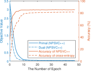
Figure 2: Training evolution of K- and D-NPSVC++.
Refer to caption
(a) ϕ(𝒙)bold-italic-ϕ𝒙{\bm{\phi}}({\bm{x}})
Refer to caption
(b) 𝒛(𝒙)𝒛𝒙{\bm{z}}({\bm{x}})
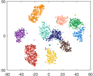
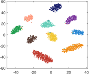
Figure 3: TSNE visualization of raw data and learned features.

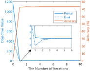
Convergence. We depict the convergence of K-NPSVC++ in Figure 2(a). The lines “primal” and “dual” refer to the objective of problem (8) and (9). Intuitively, it can be seen that the primal objective decreases rapidly and merges with the dual objective within a few steps, which indicates optimality since the dual gap becomes zero. Meanwhile, the accuracy also grows fast and becomes stable finally. Empirically, K-NPSVC++ can reach convergence within 5 iterations. Figure 2(b) shows the training evolution of D-NPSVC++. Similar to K-NPSVC++, the primal and dual objectives of D-NPSVC++ decrease monotonically and converge to a minimum. Compared with the cross-entropy, D-NPSVC++ achieves the highest accuracy within fewer epochs, which suggests that D-NPSVC++ could perform more efficient convergence than the softmax regression.

Learned features. The learned features of K-NPSVC++ are illustrated in Figure 3. It can be observed that the learned features 𝒛(𝒙)𝒛𝒙{\bm{z}}({\bm{x}}) are more discriminative than the raw features ϕ(𝒙)bold-italic-ϕ𝒙{\bm{\phi}}({\bm{x}}). The intra-class distance is squeezed and the inter-class margin is enlarged. This suggests that K-NPSVC++ can learn discriminative features and effectively improve data separability, thus further enhancing performance.
Refer to caption
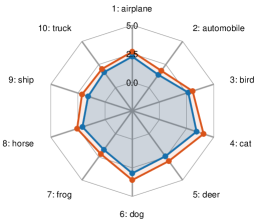
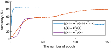
Figure 4: Ablation study of D-NPSVC++ in hypothesis function. Dashed lines indicate the convergence accuracy.

Hypothesis function. We conducted an ablation study to examine the rationality of the proposed hypothesis (6), which is compared with D-NPSVC++ trained with fl(𝒙)=𝒗l𝒛(𝒙)subscript𝑓𝑙𝒙superscriptsubscript𝒗𝑙top𝒛𝒙f_{l}({\bm{x}})={\bm{v}}_{l}^{\top}{\bm{z}}({\bm{x}}) and fl(𝒙)=𝒘lϕ(𝒙)subscript𝑓𝑙𝒙superscriptsubscript𝒘𝑙topbold-italic-ϕ𝒙f_{l}({\bm{x}})={\bm{w}}_{l}^{\top}{\bm{\phi}}({\bm{x}}), i.e., taking only one part in (6) as the compared hypothesis. As shown in Figure 4, the proposed hypothesis significantly outperforms the compared two hypotheses. Intuitively, fl(𝒙)=𝒘lϕ(𝒙)subscript𝑓𝑙𝒙superscriptsubscript𝒘𝑙topbold-italic-ϕ𝒙f_{l}({\bm{x}})={\bm{w}}_{l}^{\top}{\bm{\phi}}({\bm{x}}) performs the worst as it only depends on the features of the prior encoder. In contrast, fl(𝒙)=𝒗l𝒛(𝒙)subscript𝑓𝑙𝒙superscriptsubscript𝒗𝑙top𝒛𝒙f_{l}({\bm{x}})={\bm{v}}_{l}^{\top}{\bm{z}}({\bm{x}}) achieves a better accuracy yet converges slowly. Its reason is that D-NPSVC++ should update 𝝉𝝉{\bm{\tau}} by minimizing l=1Kτl𝒁Jlnormsuperscriptsubscript𝑙1𝐾subscript𝜏𝑙subscriptsubscript𝒁subscript𝐽𝑙\|\sum_{l=1}^{K}\tau_{l}\nabla_{{\bm{Z}}_{{\mathcal{B}}}}J_{l}\|, so the gradient is shrunk and the training is slowed consequently. Fortunately, the skip connection structure of the proposed hypothesis fl(𝒙)=𝒘lϕ(𝒙)+𝒗l𝒛(𝒙)subscript𝑓𝑙𝒙superscriptsubscript𝒘𝑙topbold-italic-ϕ𝒙superscriptsubscript𝒗𝑙top𝒛𝒙f_{l}({\bm{x}})={\bm{w}}_{l}^{\top}{\bm{\phi}}({\bm{x}})+{\bm{v}}_{l}^{\top}{\bm{z}}({\bm{x}}) can effectively avoid this phenomenon. These results sufficiently validate the efficacy of the designed hypothesis function.

6 Conclusion and Future Directions

In this paper, we establish a new classification framework, NPSVC++, which is the first end-to-end method integrating representation learning and the nonparallel classifier based on multi-objective optimization. NPSVC++ aims to achieve the Pareto optimality of multiple dependent objectives, and it theoretically ensures the optimality of the learned features across classes, solving the issues of feature suboptimality and class dependency naturally. We propose the iterative optimization framework and its two realizations, K- and D-NPSVC++, whose effectiveness is verified in experiments. NPSVCs are powerful yet underutilized classifiers in machine learning. They were born with distinctive designs compared to the mainstream classifiers. Although many works have been proposed, the inherent mechanism of NPSVC has not been well studied so far. We believe that NPSVC++ paves a new path and provides insights to investigate these classifiers. Diverse multi-objective optimization methods could be the future work, and the generalization ability of NPSVC++ is also an appealing direction.

Impact Statement

This paper provides a new learning scheme for nonparallel support vector classifiers, which makes these classifiers more applicable. The applications for classification based on deep learning and kernel method would benefit from the performance enhancement of the proposed method.

References

  • Arun Kumar & Gopal (2009) Arun Kumar, M. and Gopal, M. Least squares twin support vector machines for pattern classification. Expert Systems with Applications, 36(4):7535–7543, 2009.
  • Bai et al. (2014) Bai, L., Wang, Z., Shao, Y.-H., and Deng, N.-Y. A novel feature selection method for twin support vector machine. Knowledge-Based Systems, 59:1–8, 2014.
  • Beck (2014) Beck, A. The 2-coordinate descent method for solving double-sided simplex constrained minimization problems. Journal of Optimization Theory and Applications, 162:892–919, 2014.
  • Boyd et al. (2004) Boyd, S., Boyd, S. P., and Vandenberghe, L. Convex optimization. Cambridge University press, 2004.
  • Chandra & Bedi (2021) Chandra, M. A. and Bedi, S. Survey on SVM and their application in image classification. International Journal of Information Technology, 13:1–11, 2021.
  • Cimpoi et al. (2014) Cimpoi, M., Maji, S., Kokkinos, I., Mohamed, S., and Vedaldi, A. Describing textures in the wild. In Proceedings of the IEEE Conference on Computer Vision and Pattern Recognition, 2014.
  • Cortes & Vapnik (1995) Cortes, C. and Vapnik, V. Support-vector networks. Machine learning, 20:273–297, 1995.
  • Deng et al. (2019) Deng, J., Guo, J., Xue, N., and Zafeiriou, S. Arcface: Additive angular margin loss for deep face recognition. In Proceedings of the IEEE/CVF conference on computer vision and pattern recognition, pp.  4690–4699, 2019.
  • Diaz-Vico et al. (2020) Diaz-Vico, D., Prada, J., Omari, A., and Dorronsoro, J. Deep support vector neural networks. Integrated Computer-Aided Engineering, 27(4):389–402, 2020.
  • Dosovitskiy et al. (2020) Dosovitskiy, A., Beyer, L., Kolesnikov, A., Weissenborn, D., Zhai, X., Unterthiner, T., Dehghani, M., Minderer, M., Heigold, G., Gelly, S., et al. An image is worth 16x16 words: Transformers for image recognition at scale. In International Conference on Learning Representations, 2020.
  • Désidéri (2012) Désidéri, J.-A. Multiple-gradient descent algorithm (MGDA) for multiobjective optimization. Comptes Rendus Mathematique, 350(5-6):313–318, 2012.
  • Gao et al. (2011) Gao, S., Ye, Q., and Ye, N. 1-norm least squares twin support vector machines. Neurocomputing, 74(17):3590–3597, 2011.
  • Giagkiozis & Fleming (2015) Giagkiozis, I. and Fleming, P. Methods for multi-objective optimization: An analysis. Information Sciences, 293:338–350, 2015. ISSN 0020-0255.
  • Goudjil et al. (2018) Goudjil, M., Koudil, M., Bedda, M., and Ghoggali, N. A novel active learning method using SVM for text classification. International Journal of Automation and Computing, 15:290–298, 2018.
  • He et al. (2016) He, K., Zhang, X., Ren, S., and Sun, J. Deep residual learning for image recognition. In IEEE/CVF Conference on Computer Vision and Pattern Recognition, pp.  770–778, 2016.
  • He et al. (2005) He, X., Yan, S., Hu, Y., Niyogi, P., and Zhang, H.-J. Face recognition using laplacianfaces. IEEE Transactions on Pattern Analysis and Machine Intelligence, 27(3):328–340, 2005.
  • Jayadeva et al. (2007) Jayadeva, Khemchandani, R., and Chandra, S. Twin support vector machines for pattern classification. IEEE Transactions on Pattern Analysis and Machine Intelligence, 29(5):905–910, 2007.
  • Ke et al. (2022) Ke, J., Gong, C., Liu, T., Zhao, L., Yang, J., and Tao, D. Laplacian welsch regularization for robust semisupervised learning. IEEE Transactions on Cybernetics, 52(1):164–177, 2022.
  • Kim & Cipolla (2009) Kim, T.-K. and Cipolla, R. Canonical correlation analysis of video volume tensors for action categorization and detection. IEEE Transactions on Pattern Analysis and Machine Intelligence, 31(8):1415–1428, 2009.
  • Krizhevsky (2009) Krizhevsky, A. Learning multiple layers of features from tiny images. Technical report, 2009.
  • Li & Yang (2022) Li, M. and Yang, Z. Deep twin support vector networks. In Artificial Intelligence, pp.  94–106, 2022.
  • Liu et al. (2022) Liu, Z., Mao, H., Wu, C.-Y., Feichtenhofer, C., Darrell, T., and Xie, S. A convnet for the 2020s. In Proceedings of the IEEE/CVF conference on computer vision and pattern recognition, pp.  11976–11986, 2022.
  • Loshchilov & Hutter (2016) Loshchilov, I. and Hutter, F. SGDR: Stochastic gradient descent with warm restarts. In International Conference on Learning Representations, 2016.
  • Majeed & Alkhafaji (2023) Majeed, R. R. and Alkhafaji, S. K. D. ECG classification system based on multi-domain features approach coupled with least square support vector machine (LS-SVM). Computer Methods in Biomechanics and Biomedical Engineering, 26(5):540–547, 2023.
  • Mangasarian & Wild (2006) Mangasarian, O. and Wild, E. Multisurface proximal support vector machine classification via generalized eigenvalues. IEEE Transactions on Pattern Analysis and Machine Intelligence, 28(1):69–74, 2006.
  • Mao et al. (2023) Mao, A., Mohri, M., and Zhong, Y. Cross-entropy loss functions: Theoretical analysis and applications. In Proceedings of the 40th International Conference on Machine Learning, pp.  23803–23828, 2023.
  • Mohri et al. (2018) Mohri, M., Rostamizadeh, A., and Talwalkar, A. Foundations of machine learning. MIT press, 2018.
  • Momma et al. (2022) Momma, M., Dong, C., and Liu, J. A multi-objective/multi-task learning framework induced by Pareto stationarity. In International Conference on Machine Learning, pp.  15895–15907, 2022.
  • Nie et al. (2017) Nie, F., Zhang, R., and Li, X. A generalized power iteration method for solving quadratic problem on the stiefel manifold. Science China Information Sciences, 60:273–297, 2017.
  • Nilsback & Zisserman (2008) Nilsback, M.-E. and Zisserman, A. Automated flower classification over a large number of classes. In Indian Conference on Computer Vision, Graphics and Image Processing, Dec 2008.
  • Schölkopf et al. (2002) Schölkopf, B., Smola, A. J., Bach, F., et al. Learning with kernels: support vector machines, regularization, optimization, and beyond. MIT press, 2002.
  • Sener & Koltun (2018) Sener, O. and Koltun, V. Multi-task learning as multi-objective optimization. In Advances in Neural Information Processing Systems, 2018.
  • Shao et al. (2011) Shao, Y.-H., Zhang, C.-H., Wang, X.-B., and Deng, N.-Y. Improvements on twin support vector machines. IEEE Transactions on Neural Networks, 22(6):962–968, 2011.
  • Shao et al. (2014) Shao, Y.-H., Chen, W.-J., and Deng, N.-Y. Nonparallel hyperplane support vector machine for binary classification problems. Information Sciences, 263:22–35, 2014.
  • Simonyan & Zisserman (2015) Simonyan, K. and Zisserman, A. Very deep convolutional networks for large-scale image recognition. In International Conference on Learning Representations, pp.  1–14, 2015.
  • Suykens & Vandewalle (1999) Suykens, J. A. and Vandewalle, J. Least squares support vector machine classifiers. Neural Processing Letters, 9(3):293–300, 1999.
  • Tanveer et al. (2019) Tanveer, M., Sharma, A., and Suganthan, P. General twin support vector machine with pinball loss function. Information Sciences, 494:311–327, 2019.
  • Tian et al. (2014) Tian, Y., Qi, Z., Ju, X., Shi, Y., and Liu, X. Nonparallel support vector machines for pattern classification. IEEE Transactions on Cybernetics, 44(7):1067–1079, 2014.
  • Vaswani et al. (2017) Vaswani, A., Shazeer, N., Parmar, N., Uszkoreit, J., Jones, L., Gomez, A. N., Kaiser, L. u., and Polosukhin, I. Attention is all you need. In Advances in Neural Information Processing Systems, 2017.
  • Wang et al. (2018) Wang, F., Cheng, J., Liu, W., and Liu, H. Additive margin softmax for face verification. IEEE Signal Processing Letters, 25(7):926–930, 2018.
  • Wang et al. (2019) Wang, J., Feng, K., and Wu, J. SVM-based deep stacking networks. In Proceedings of the AAAI conference on artificial intelligence, volume 33, pp.  5273–5280, 2019.
  • Wen & Yin (2013) Wen, Z. and Yin, W. A feasible method for optimization with orthogonality constraints. Mathematical Programming, 142(1):397–434, 2013.
  • Xie et al. (2020) Xie, D., Nie, F., and Gao, Q. On the optimal solution to maximum margin projection pursuit. Multimedia Tools and Applications, 79:35441–35461, 2020.
  • Xie et al. (2013) Xie, J., Hone, K., Xie, W., Gao, X., Shi, Y., and Liu, X. Extending twin support vector machine classifier for multi-category classification problems. Intelligent Data Analysis, 17(4):649–664, 2013.
  • Xie et al. (2023) Xie, X., Li, Y., and Sun, S. Deep multi-view multiclass twin support vector machines. Information Fusion, 91:80–92, 2023.
  • Xu et al. (2017) Xu, Y., Yang, Z., and Pan, X. A novel twin support-vector machine with pinball loss. IEEE Transactions on Neural Networks and Learning Systems, 28(2):359–370, 2017.
  • Yuan et al. (2021) Yuan, C., Yang, L., and Sun, P. Correntropy-based metric for robust twin support vector machine. Information Sciences, 545:82–101, 2021.
  • Zhang et al. (2023) Zhang, J., Lai, Z., Kong, H., and Shen, L. Robust twin bounded support vector classifier with manifold regularization. IEEE Transactions on Cybernetics, 53(8):5135–5150, 2023.
  • Zou et al. (2006) Zou, H., Hastie, T., and Tibshirani, R. Sparse principal component analysis. Journal of computational and graphical statistics, pp.  265–286, 2006.

Appendix A Proof of Theorem 1

Proof.

We first rewrite weighted Chebyshev problem as

minρ,𝜽ρ,s.t.𝑱(𝜽)ρ𝟏.formulae-sequencesubscript𝜌𝜽𝜌st𝑱𝜽𝜌1\min_{\rho,{\bm{\theta}}}~{}\rho,\quad\mathrm{s.t.}~{}\bm{J}({\bm{\theta}})\leq\rho{\bm{1}}. (A.1)

Then its Lagrangte function is

L(ρ,𝜽,𝝉)=ρ+𝝉(𝑱(𝜽)ρ𝟏).𝐿𝜌𝜽𝝉𝜌superscript𝝉top𝑱𝜽𝜌1L(\rho,{\bm{\theta}},{\bm{\tau}})=\rho+{\bm{\tau}}^{\top}(\bm{J}({\bm{\theta}})-\rho{\bm{1}}). (A.2)

By KKT conditions, we have

ρLsubscript𝜌𝐿\displaystyle\nabla_{\rho}L =1𝝉𝟏=0absent1superscript𝝉top10\displaystyle=1-{\bm{\tau}}^{\top}{\bm{1}}=0
𝜽Lsubscript𝜽𝐿\displaystyle\nabla_{{\bm{\theta}}}L =𝜽𝑱𝝉=l=1Kτl𝜽Jl=𝟎,τl0,l[K].formulae-sequenceabsentsubscript𝜽𝑱𝝉superscriptsubscript𝑙1𝐾subscript𝜏𝑙subscript𝜽subscript𝐽𝑙0formulae-sequencesubscript𝜏𝑙0for-all𝑙delimited-[]𝐾\displaystyle=\nabla_{\bm{\theta}}\bm{J}{\bm{\tau}}=\sum_{l=1}^{K}\tau_{l}\nabla_{{\bm{\theta}}}J_{l}=\bm{0},\quad\tau_{l}\geq 0,\forall l\in[K].

where 𝜽𝑱=[𝜽J1,𝜽J2,,𝜽JK]subscript𝜽𝑱subscript𝜽subscript𝐽1subscript𝜽subscript𝐽2subscript𝜽subscript𝐽𝐾\nabla_{\bm{\theta}}\bm{J}=[\nabla_{{\bm{\theta}}}J_{1},\nabla_{{\bm{\theta}}}J_{2},\cdots,\nabla_{{\bm{\theta}}}J_{K}]. Therefore, the dual problem is formulated as

max𝝉min𝜽,ρL(ρ,𝜽,𝝉)subscript𝝉subscript𝜽𝜌𝐿𝜌𝜽𝝉\displaystyle\mathrel{\phantom{=}}\max_{{\bm{\tau}}}\min_{{\bm{\theta}},\rho}L(\rho,{\bm{\theta}},{\bm{\tau}})
=max𝝉min𝜽,ρρ(1𝝉𝟏)+𝝉𝑱(𝜽)absentsubscript𝝉subscript𝜽𝜌𝜌1superscript𝝉top1superscript𝝉top𝑱𝜽\displaystyle=\max_{{\bm{\tau}}}\min_{{\bm{\theta}},\rho}\rho(1-{\bm{\tau}}^{\top}{\bm{1}})+{\bm{\tau}}^{\top}\bm{J}({\bm{\theta}})
=max𝝉min𝜽𝝉𝑱(𝜽),absentsubscript𝝉subscript𝜽superscript𝝉top𝑱𝜽\displaystyle=\max_{{\bm{\tau}}}\min_{{\bm{\theta}}}{\bm{\tau}}^{\top}\bm{J}({\bm{\theta}}),
s.t.l=1Kτl𝜽Jl=𝟎,τl0,𝝉𝟏=1.formulae-sequencestformulae-sequencesuperscriptsubscript𝑙1𝐾subscript𝜏𝑙subscript𝜽subscript𝐽𝑙0formulae-sequencesubscript𝜏𝑙0superscript𝝉top11\displaystyle\mathrm{s.t.}~{}\sum_{l=1}^{K}\tau_{l}\nabla_{{\bm{\theta}}}J_{l}=\bm{0},~{}\tau_{l}\geq 0,~{}{\bm{\tau}}^{\top}{\bm{1}}=1.

Besides, let 𝜽lsubscript𝜽𝑙{\bm{\theta}}_{l} be the specific variable of objective Jlsubscript𝐽𝑙J_{l}, and 𝜽shsubscript𝜽𝑠{\bm{\theta}}_{sh} be the variable shared to all objectives. By the optimality condition of minimization problem min𝜽𝝉𝑱(𝜽)subscript𝜽superscript𝝉top𝑱𝜽\min_{{\bm{\theta}}}{\bm{\tau}}^{\top}\bm{J}({\bm{\theta}}), we have

𝜽lJl(𝜽)=𝟎,l[K].formulae-sequencesubscriptsubscript𝜽𝑙subscript𝐽𝑙𝜽0for-all𝑙delimited-[]𝐾\nabla_{{\bm{\theta}}_{l}}J_{l}({\bm{\theta}})=\bm{0},~{}\forall l\in[K].
l=1Kτl𝜽Jlsuperscriptsubscript𝑙1𝐾subscript𝜏𝑙subscript𝜽subscript𝐽𝑙\displaystyle\sum_{l=1}^{K}\tau_{l}\nabla_{{\bm{\theta}}}J_{l} =[𝜽1J1𝜽2J2𝜽KJK𝜽shJ1𝜽shJ2𝜽shJK]𝝉absentmatrixsubscriptsubscript𝜽1subscript𝐽1subscriptsubscript𝜽2subscript𝐽2subscriptsubscript𝜽𝐾subscript𝐽𝐾subscriptsubscript𝜽𝑠subscript𝐽1subscriptsubscript𝜽𝑠subscript𝐽2subscriptsubscript𝜽𝑠subscript𝐽𝐾𝝉\displaystyle=\begin{bmatrix}\nabla_{{\bm{\theta}}_{1}}J_{1}&\nabla_{{\bm{\theta}}_{2}}J_{2}&\cdots&\nabla_{{\bm{\theta}}_{K}}J_{K}\\ \nabla_{{\bm{\theta}}_{sh}}J_{1}&\nabla_{{\bm{\theta}}_{sh}}J_{2}&\cdots&\nabla_{{\bm{\theta}}_{sh}}J_{K}\end{bmatrix}{\bm{\tau}}
=[𝟎𝟎𝟎𝜽shJ1𝜽shJ2𝜽shJK]𝝉=[𝟎𝟎],absentmatrix000subscriptsubscript𝜽𝑠subscript𝐽1subscriptsubscript𝜽𝑠subscript𝐽2subscriptsubscript𝜽𝑠subscript𝐽𝐾𝝉matrix00\displaystyle=\begin{bmatrix}\bm{0}&\bm{0}&\cdots&\bm{0}\\ \nabla_{{\bm{\theta}}_{sh}}J_{1}&\nabla_{{\bm{\theta}}_{sh}}J_{2}&\cdots&\nabla_{{\bm{\theta}}_{sh}}J_{K}\end{bmatrix}{\bm{\tau}}=\begin{bmatrix}\bm{0}\\ \bm{0}\end{bmatrix},

we only need to guarantee the constraints:

l=1Kτl𝜽shJl=𝟎.superscriptsubscript𝑙1𝐾subscript𝜏𝑙subscriptsubscript𝜽𝑠subscript𝐽𝑙0\sum_{l=1}^{K}\tau_{l}\nabla_{{\bm{\theta}}_{sh}}J_{l}=\bm{0}.

Thus, the desired result is obtained. ∎

Appendix B Derivation of 𝒖𝒖{\bm{u}}-step update.

𝒖lsubscript𝒖𝑙{\bm{u}}_{l} step. By introducing slack variable 𝝃lsubscript𝝃𝑙{\bm{\xi}}_{l}, we obtain the following problem that optimizes 𝒖lsubscript𝒖𝑙{\bm{u}}_{l}:

min𝜷l,𝝃lsubscriptsubscript𝜷𝑙subscript𝝃𝑙\displaystyle\min_{{\bm{\beta}}_{l},{\bm{\xi}}_{l}} 12𝑲l𝜷2+c𝟏𝝃l+r12(𝜷l𝑲𝜷l2𝜷l𝑲𝑨𝒗l)12superscriptnormsuperscriptsubscript𝑲𝑙top𝜷2𝑐superscript1topsubscript𝝃𝑙subscript𝑟12superscriptsubscript𝜷𝑙top𝑲subscript𝜷𝑙2superscriptsubscript𝜷𝑙top𝑲𝑨subscript𝒗𝑙\displaystyle~{}\frac{1}{2}\|{\bm{K}}_{l}^{\top}{\bm{\beta}}\|^{2}+c{\bm{1}}^{\top}{\bm{\xi}}_{l}+\frac{r_{1}}{2}({\bm{\beta}}_{l}^{\top}{\bm{K}}{\bm{\beta}}_{l}-2{\bm{\beta}}_{l}^{\top}{\bm{K}}{\bm{A}}{\bm{v}}_{l})
s.t.formulae-sequencest\displaystyle\mathrm{s.t.}~{} 𝟏𝝃l𝑲l𝜷l𝟎,𝝃l𝟎,formulae-sequence1subscript𝝃𝑙superscriptsubscript𝑲𝑙topsubscript𝜷𝑙0subscript𝝃𝑙0\displaystyle{\bm{1}}-{\bm{\xi}}_{l}-{\bm{K}}_{-l}^{\top}{\bm{\beta}}_{l}\leq\bm{0},\quad{\bm{\xi}}_{l}\geq\bm{0}, (A.3)

where 𝑲l=[𝜿i]yilsubscript𝑲𝑙subscriptdelimited-[]subscript𝜿𝑖subscript𝑦𝑖𝑙{\bm{K}}_{-l}=[\bm{\kappa}_{i}]_{y_{i}\not=l}. To cope with the inequality constraints, the Lagrange function is introduced:

L(𝒖l,𝝃l,𝝀,𝝂)𝐿subscript𝒖𝑙subscript𝝃𝑙𝝀𝝂\displaystyle L({\bm{u}}_{l},{\bm{\xi}}_{l},{\bm{\lambda}},{\bm{\nu}}) =12𝑲l𝜷2+c𝟏𝝃l+r12(𝜷l𝑲𝜷l2𝜷l𝑲𝑨𝒗l)absent12superscriptnormsuperscriptsubscript𝑲𝑙top𝜷2𝑐superscript1topsubscript𝝃𝑙subscript𝑟12superscriptsubscript𝜷𝑙top𝑲subscript𝜷𝑙2superscriptsubscript𝜷𝑙top𝑲𝑨subscript𝒗𝑙\displaystyle=\frac{1}{2}\|{\bm{K}}_{l}^{\top}{\bm{\beta}}\|^{2}+c{\bm{1}}^{\top}{\bm{\xi}}_{l}+\frac{r_{1}}{2}({\bm{\beta}}_{l}^{\top}{\bm{K}}{\bm{\beta}}_{l}-2{\bm{\beta}}_{l}^{\top}{\bm{K}}{\bm{A}}{\bm{v}}_{l})
+𝝀(𝟏𝝃l𝑲l𝜷l)𝝂𝝃,superscript𝝀top1subscript𝝃𝑙superscriptsubscript𝑲𝑙topsubscript𝜷𝑙superscript𝝂top𝝃\displaystyle+{\bm{\lambda}}^{\top}({\bm{1}}-{\bm{\xi}}_{l}-{\bm{K}}_{-l}^{\top}{\bm{\beta}}_{l})-{\bm{\nu}}^{\top}{\bm{\xi}}, (A.4)

where 𝝀𝝀{\bm{\lambda}} and 𝝂𝝂{\bm{\nu}} are non-negative Lagrange multipliers. According to Karush-Kuhn-Tucker (KKT) optimality conditions,

𝒖lLsubscriptsubscript𝒖𝑙𝐿\displaystyle\nabla_{{\bm{u}}_{l}}L =𝑲l𝑲l𝒖l+r1(𝑲𝜷l𝑲𝑨𝒗l)𝑲l𝝀=𝟎absentsubscript𝑲𝑙superscriptsubscript𝑲𝑙topsubscript𝒖𝑙subscript𝑟1𝑲subscript𝜷𝑙𝑲𝑨subscript𝒗𝑙subscript𝑲𝑙𝝀0\displaystyle={\bm{K}}_{l}{\bm{K}}_{l}^{\top}{\bm{u}}_{l}+r_{1}({\bm{K}}{\bm{\beta}}_{l}-{\bm{K}}{\bm{A}}{\bm{v}}_{l})-{\bm{K}}_{-l}{\bm{\lambda}}=\bm{0}
𝝃Lsubscript𝝃𝐿\displaystyle\nabla_{{\bm{\xi}}}L =c𝟏𝝀𝝂=𝟎.absent𝑐1𝝀𝝂0\displaystyle=c{\bm{1}}-{\bm{\lambda}}-{\bm{\nu}}=\bm{0}.

Thus the closed-form solution to 𝒖lsubscript𝒖𝑙{\bm{u}}_{l} is given by:

𝜷l=(𝑲l𝑲l+r1𝑲)1(r1𝑲𝑨𝒗l𝑲l𝝀l).subscript𝜷𝑙superscriptsubscript𝑲𝑙superscriptsubscript𝑲𝑙topsubscript𝑟1𝑲1subscript𝑟1𝑲𝑨subscript𝒗𝑙subscript𝑲𝑙subscript𝝀𝑙{\bm{\beta}}_{l}=({\bm{K}}_{l}{\bm{K}}_{l}^{\top}+r_{1}{\bm{K}})^{-1}(r_{1}{\bm{K}}{\bm{A}}{\bm{v}}_{l}-{\bm{K}}_{-l}{\bm{\lambda}}_{l}). (A.5)

Plugging the above results into the Lagrange function and with some simple algebra, we derive the dual problem of the primal problem (A.3):

max𝝀,𝝂min𝒖l,𝝃L(𝒖l,𝝃,𝝀,𝝂)s.t.λi0,νi0formulae-sequencesubscript𝝀𝝂subscriptsubscript𝒖𝑙𝝃𝐿subscript𝒖𝑙𝝃𝝀𝝂stformulae-sequencesubscript𝜆𝑖0subscript𝜈𝑖0\displaystyle\max_{{\bm{\lambda}},{\bm{\nu}}}\min_{{\bm{u}}_{l},{\bm{\xi}}}L({\bm{u}}_{l},{\bm{\xi}},{\bm{\lambda}},{\bm{\nu}})\quad\mathrm{s.t.}~{}\lambda_{i}\geq 0,\nu_{i}\geq 0
\displaystyle\Leftrightarrow min𝝀12𝝀l𝑲l𝑴l𝑲l𝝀l+(r1𝑲l𝑴l𝑲𝑨𝒗l𝟏)𝝀l,subscript𝝀12superscriptsubscript𝝀𝑙topsuperscriptsubscript𝑲𝑙topsubscript𝑴𝑙subscript𝑲𝑙subscript𝝀𝑙superscriptsubscript𝑟1superscriptsubscript𝑲𝑙topsubscript𝑴𝑙𝑲𝑨subscript𝒗𝑙1topsubscript𝝀𝑙\displaystyle\min_{{\bm{\lambda}}}\frac{1}{2}{\bm{\lambda}}_{l}^{\top}{\bm{K}}_{-l}^{\top}{\bm{M}}_{l}{\bm{K}}_{-l}{\bm{\lambda}}_{l}+\left(r_{1}{\bm{K}}_{l}^{\top}{\bm{M}}_{l}{\bm{K}}{\bm{A}}{\bm{v}}_{l}-{\bm{1}}\right)^{\top}{\bm{\lambda}}_{l},
s.t.0λic.formulae-sequencest0subscript𝜆𝑖𝑐\displaystyle~{}\mathrm{s.t.}~{}0\leq\lambda_{i}\leq c. (A.6)

where 𝑴l=(𝑲l𝑲l+r1𝑲)1subscript𝑴𝑙superscriptsubscript𝑲𝑙superscriptsubscript𝑲𝑙topsubscript𝑟1𝑲1{\bm{M}}_{l}=({\bm{K}}_{l}{\bm{K}}_{l}^{\top}+r_{1}{\bm{K}})^{-1}.

Note that the computation of 𝑴lsubscript𝑴𝑙{\bm{M}}_{l} requires matrix inversion and thus costs O(n3)𝑂superscript𝑛3O(n^{3}) time. To simplify the computation, we first introduce three auxiliary matrices:

𝑸K,K(l)subscriptsuperscript𝑸𝑙𝐾𝐾\displaystyle{\bm{Q}}^{(l)}_{K,K} =𝑲l𝑴l𝑲l,𝑸Ψ,Ψ(l)=𝚿𝑴l𝚿,formulae-sequenceabsentsubscript𝑲𝑙subscript𝑴𝑙superscriptsubscript𝑲𝑙topsubscriptsuperscript𝑸𝑙ΨΨsuperscript𝚿topsubscript𝑴𝑙𝚿\displaystyle={\bm{K}}_{-l}{\bm{M}}_{l}{\bm{K}}_{-l}^{\top},\quad{\bm{Q}}^{(l)}_{\Psi,\Psi}={\bm{\Psi}}^{\top}{\bm{M}}_{l}{\bm{\Psi}}, (A.7)
𝑸K,Ψ(l)subscriptsuperscript𝑸𝑙𝐾Ψ\displaystyle{\bm{Q}}^{(l)}_{K,\Psi} =𝚿𝑴l𝑲l.absentsuperscript𝚿topsubscript𝑴𝑙subscript𝑲𝑙\displaystyle={\bm{\Psi}}^{\top}{\bm{M}}_{l}{\bm{K}}_{-l}.

Then by (A.5) and the definition of 𝑼^^𝑼\widehat{\bm{U}}, we have

𝒖^l=r1𝑸Ψ,Ψ(l)𝑷^𝒗l+𝑸K,Ψ(l)𝝀l,subscript^𝒖𝑙subscript𝑟1subscriptsuperscript𝑸𝑙ΨΨ^𝑷subscript𝒗𝑙subscriptsuperscript𝑸𝑙𝐾Ψsubscript𝝀𝑙\widehat{\bm{u}}_{l}=r_{1}{\bm{Q}}^{(l)}_{\Psi,\Psi}\widehat{\bm{P}}{\bm{v}}_{l}+{\bm{Q}}^{(l)}_{K,\Psi}{\bm{\lambda}}_{l}, (A.8)

where 𝝀+nl𝝀subscriptsuperscriptsubscript𝑛𝑙{\bm{\lambda}}\in{\mathbb{R}}^{n_{l}}_{+} denotes the Lagrange multiplier and is obtained by the following dual problem:

min𝟎𝝀lc𝟏12𝝀l𝑸K,K(l)𝝀l+(𝑸K,Ψ(l)𝑷^𝒗l𝟏)𝝀l.subscript0subscript𝝀𝑙𝑐112superscriptsubscript𝝀𝑙topsubscriptsuperscript𝑸𝑙𝐾𝐾subscript𝝀𝑙superscriptsubscriptsuperscript𝑸𝑙𝐾Ψ^𝑷subscript𝒗𝑙1topsubscript𝝀𝑙\min_{\bm{0}\leq{\bm{\lambda}}_{l}\leq c{\bm{1}}}\frac{1}{2}{\bm{\lambda}}_{l}^{\top}{\bm{Q}}^{(l)}_{K,K}{\bm{\lambda}}_{l}+({\bm{Q}}^{(l)}_{K,\Psi}\widehat{\bm{P}}{\bm{v}}_{l}-{\bm{1}})^{\top}{\bm{\lambda}}_{l}. (A.9)

Now we show how to compute the frequently used matrices (A.7). Using the Woodbury formula (Ke et al., 2022), we rewrite 𝑴lsubscript𝑴𝑙{\bm{M}}_{l} as

(𝑲l𝑲l+r1𝑲)1superscriptsubscript𝑲𝑙superscriptsubscript𝑲𝑙topsubscript𝑟1𝑲1\displaystyle\mathrel{\phantom{=}}({\bm{K}}_{l}{\bm{K}}_{l}^{\top}+r_{1}{\bm{K}})^{-1}
=1r1𝑲11r12𝑲1𝑲l(𝑰+1r1𝑲l𝑲1𝑲l)1𝑲l𝑲1absent1subscript𝑟1superscript𝑲11superscriptsubscript𝑟12superscript𝑲1subscript𝑲𝑙superscript𝑰1subscript𝑟1superscriptsubscript𝑲𝑙topsuperscript𝑲1subscript𝑲𝑙1superscriptsubscript𝑲𝑙topsuperscript𝑲1\displaystyle=\frac{1}{r_{1}}{\bm{K}}^{-1}-\frac{1}{r_{1}^{2}}{\bm{K}}^{-1}{\bm{K}}_{l}\left({\bm{I}}+\frac{1}{r_{1}}{\bm{K}}_{l}^{\top}{\bm{K}}^{-1}{\bm{K}}_{l}\right)^{-1}{\bm{K}}_{l}^{\top}{\bm{K}}^{-1}
=1r1[𝑲1𝑲1𝑲l(r1𝑰+𝑲l𝑲1𝑲l)1𝑲l𝑲1].absent1subscript𝑟1delimited-[]superscript𝑲1superscript𝑲1subscript𝑲𝑙superscriptsubscript𝑟1𝑰superscriptsubscript𝑲𝑙topsuperscript𝑲1subscript𝑲𝑙1superscriptsubscript𝑲𝑙topsuperscript𝑲1\displaystyle=\frac{1}{r_{1}}\left[{\bm{K}}^{-1}-{\bm{K}}^{-1}{\bm{K}}_{l}\left(r_{1}{\bm{I}}+{\bm{K}}_{l}^{\top}{\bm{K}}^{-1}{\bm{K}}_{l}\right)^{-1}{\bm{K}}_{l}^{\top}{\bm{K}}^{-1}\right].

Remind the Cholesky decomposition 𝑲=𝚿𝚿𝑲𝚿superscript𝚿top{\bm{K}}={\bm{\Psi}}{\bm{\Psi}}^{\top}, and thus 𝑲1=𝚿𝚿1superscript𝑲1superscript𝚿absenttopsuperscript𝚿1{\bm{K}}^{-1}={\bm{\Psi}}^{-\top}{\bm{\Psi}}^{-1}. Then we have

𝑲l𝑲1𝑲l=𝚿l𝚿(𝚿𝚿1)𝚿𝚿l=𝚿l𝚿l,superscriptsubscript𝑲𝑙topsuperscript𝑲1subscript𝑲𝑙subscript𝚿𝑙superscript𝚿topsuperscript𝚿absenttopsuperscript𝚿1𝚿superscriptsubscript𝚿𝑙topsubscript𝚿𝑙superscriptsubscript𝚿𝑙top{\bm{K}}_{l}^{\top}{\bm{K}}^{-1}{\bm{K}}_{l}={\bm{\Psi}}_{l}{\bm{\Psi}}^{\top}({\bm{\Psi}}^{-\top}{\bm{\Psi}}^{-1}){\bm{\Psi}}{\bm{\Psi}}_{l}^{\top}={\bm{\Psi}}_{l}{\bm{\Psi}}_{l}^{\top}, (A.10)

where 𝚿lnl×nsubscript𝚿𝑙superscriptsubscript𝑛𝑙𝑛{\bm{\Psi}}_{l}\in{\mathbb{R}}^{n_{l}\times n} is comprised of the rows of 𝚿𝚿{\bm{\Psi}} corresponding to the l𝑙l-th class. Likewise, we have 𝑲l𝑲1𝑲l=𝚿l𝚿lsuperscriptsubscript𝑲𝑙topsuperscript𝑲1subscript𝑲𝑙subscript𝚿𝑙subscriptsuperscript𝚿top𝑙{\bm{K}}_{-l}^{\top}{\bm{K}}^{-1}{\bm{K}}_{-l}={\bm{\Psi}}_{-l}{\bm{\Psi}}^{\top}_{-l}. Therefore, the following equations hold:

𝑸Ψ,Ψ(l)subscriptsuperscript𝑸𝑙ΨΨ\displaystyle{\bm{Q}}^{(l)}_{\Psi,\Psi} =1r1[𝑰𝚿l(r1𝑰+𝚿l𝚿l)1𝚿l],absent1subscript𝑟1delimited-[]𝑰superscriptsubscript𝚿𝑙topsuperscriptsubscript𝑟1𝑰subscript𝚿𝑙superscriptsubscript𝚿𝑙top1subscript𝚿𝑙\displaystyle=\frac{1}{r_{1}}\left[{\bm{I}}-{\bm{\Psi}}_{l}^{\top}(r_{1}{\bm{I}}+{\bm{\Psi}}_{l}{\bm{\Psi}}_{l}^{\top})^{-1}{\bm{\Psi}}_{l}\right], (A.11)
𝑸K,Ψ(l)subscriptsuperscript𝑸𝑙𝐾Ψ\displaystyle{\bm{Q}}^{(l)}_{K,\Psi} =𝚿l𝑸Ψ,Ψ(l),𝑸K,K(l)=𝚿l𝑸Ψ,Ψ(l)𝚿l,formulae-sequenceabsentsuperscriptsubscript𝚿𝑙topsubscriptsuperscript𝑸𝑙ΨΨsubscriptsuperscript𝑸𝑙𝐾𝐾superscriptsubscript𝚿𝑙topsubscriptsuperscript𝑸𝑙ΨΨsubscript𝚿𝑙\displaystyle={\bm{\Psi}}_{-l}^{\top}{\bm{Q}}^{(l)}_{\Psi,\Psi},\quad{\bm{Q}}^{(l)}_{K,K}={\bm{\Psi}}_{-l}^{\top}{\bm{Q}}^{(l)}_{\Psi,\Psi}{\bm{\Psi}}_{-l},

Therefore, the size of matrix inversion is decreased to nlsubscript𝑛𝑙n_{l}, which will significantly reduce the computation burden.

Appendix C Details of the Algorithms and Implementations

C.1 Algorithms

The detailed training procedures are shown in Algorithm 1 and 2.

Algorithm 1 Training K-NPSVC++

Input: Samples 𝑿m×n,𝒚[K]nformulae-sequence𝑿superscript𝑚𝑛𝒚superscriptdelimited-[]𝐾𝑛{\bm{X}}\in{\mathbb{R}}^{m\times n},{\bm{y}}\in[K]^{n}.
Output: Matrix 𝑼^n×K^𝑼superscript𝑛𝐾\widehat{\bm{U}}\in{\mathbb{R}}^{n\times K}, 𝑽d×K𝑽superscript𝑑𝐾{\bm{V}}\in{\mathbb{R}}^{d\times K}, and projection matrix 𝑷^n×d^𝑷superscript𝑛𝑑\widehat{\bm{P}}\in{\mathbb{R}}^{n\times d}.

1:  Initialize 𝑼^0,𝑽0,𝑷^0subscript^𝑼0subscript𝑽0subscript^𝑷0\widehat{\bm{U}}_{0},{\bm{V}}_{0},\widehat{\bm{P}}_{0} such that 𝑷^0𝑷^0=𝑰superscriptsubscript^𝑷0topsubscript^𝑷0𝑰\widehat{\bm{P}}_{0}^{\top}\widehat{\bm{P}}_{0}={\bm{I}}, and 𝝉0=𝟏/Ksubscript𝝉01𝐾{\bm{\tau}}_{0}={\bm{1}}/K.
2:  Let t0𝑡0t\leftarrow 0.
3:  if “Linear kernel” is used then
4:     Let 𝚿𝑿𝚿superscript𝑿top{\bm{\Psi}}\leftarrow{\bm{X}}^{\top}
5:  else
6:     Compute the kernel matrix 𝑲=𝒦(𝑿,𝑿)+ϵ𝑰𝑲𝒦𝑿𝑿italic-ϵ𝑰{\bm{K}}={\mathcal{K}}({\bm{X}},{\bm{X}})+\epsilon{\bm{I}} and
7:     Compute the Cholesky decomposition 𝚿𝚿=𝑲𝚿superscript𝚿top𝑲{\bm{\Psi}}{\bm{\Psi}}^{\top}={\bm{K}}.
8:  end if
9:  Compute 𝑯μ𝚿𝑳𝚿𝑯𝜇superscript𝚿top𝑳𝚿{\bm{H}}\leftarrow\mu{\bm{\Psi}}^{\top}{\bm{L}}{\bm{\Psi}}.
10:  Compute 𝑸Ψ,Ψ(l)subscriptsuperscript𝑸𝑙ΨΨ{\bm{Q}}^{(l)}_{\Psi,\Psi}, 𝑸Ψ,K(l)subscriptsuperscript𝑸𝑙Ψ𝐾{\bm{Q}}^{(l)}_{\Psi,K} and 𝑸K,K(l)subscriptsuperscript𝑸𝑙𝐾𝐾{\bm{Q}}^{(l)}_{K,K} for l[K]𝑙delimited-[]𝐾l\in[K] via (14).
11:  while t<MAX_ITER𝑡MAX_ITERt<\text{MAX\_ITER} and not convergent do
12:     for l[K]𝑙delimited-[]𝐾l\in[K] do
13:        Solve the problem (A.9).
14:        Update 𝒖^t+1,lr1𝑸Ψ,Ψ(l)𝑷^t𝒗t,l+𝑸K,Ψ(l)𝝀lsubscript^𝒖𝑡1𝑙subscript𝑟1subscriptsuperscript𝑸𝑙ΨΨsubscript^𝑷𝑡subscript𝒗𝑡𝑙subscriptsuperscript𝑸𝑙𝐾Ψsubscript𝝀𝑙\widehat{\bm{u}}_{t+1,l}\leftarrow r_{1}{\bm{Q}}^{(l)}_{\Psi,\Psi}\widehat{\bm{P}}_{t}{\bm{v}}_{t,l}+{\bm{Q}}^{(l)}_{K,\Psi}{\bm{\lambda}}_{l}.
15:     end for
16:     Update 𝑽t+1r1𝑷^t𝑼^t+1/(r1+r2)subscript𝑽𝑡1subscript𝑟1superscriptsubscript^𝑷𝑡topsubscript^𝑼𝑡1subscript𝑟1subscript𝑟2{\bm{V}}_{t+1}\leftarrow r_{1}\widehat{\bm{P}}_{t}^{\top}\widehat{\bm{U}}_{t+1}/(r_{1}+r_{2}).
17:     Update 𝑬r1𝑼^t+1diag(𝝉t)𝑽t+1𝑬subscript𝑟1subscript^𝑼𝑡1diagsubscript𝝉𝑡superscriptsubscript𝑽𝑡1top{\bm{E}}\leftarrow r_{1}\widehat{\bm{U}}_{t+1}\mathrm{diag}({\bm{\tau}}_{t}){\bm{V}}_{t+1}^{\top}.
18:     Update 𝑷^t+12𝖦𝖯𝖨(𝑯,𝑬,𝑷t)subscript^𝑷𝑡12𝖦𝖯𝖨𝑯𝑬subscript𝑷𝑡\widehat{\bm{P}}_{t+\frac{1}{2}}\leftarrow\mathsf{GPI}({\bm{H}},{\bm{E}},{\bm{P}}_{t}) with Algorithm by (Nie et al., 2017).
19:     Update 𝝉t+1subscript𝝉𝑡1{\bm{\tau}}_{t+1} by solving QPP (20).
20:     Let 𝑷^t+1𝝅𝖲𝗍(𝑷^t+12ηl=1Kτt+1,l𝑷^t+12𝖲𝗍Jl)subscript^𝑷𝑡1subscript𝝅𝖲𝗍subscript^𝑷𝑡12𝜂superscriptsubscript𝑙1𝐾subscript𝜏𝑡1𝑙superscriptsubscriptsubscript^𝑷𝑡12𝖲𝗍subscript𝐽𝑙\widehat{\bm{P}}_{t+1}\leftarrow{\bm{\pi}}_{\mathsf{St}}\left(\widehat{\bm{P}}_{t+\frac{1}{2}}-\eta\sum_{l=1}^{K}\tau_{t+1,l}\nabla_{\widehat{\bm{P}}_{t+\frac{1}{2}}}^{\mathsf{St}}J_{l}\right).
21:     Let tt+1𝑡𝑡1t\leftarrow t+1.
22:  end while
Algorithm 2 Training D-NPSVC++
1:  for p=1:nepoch:𝑝1subscript𝑛𝑒𝑝𝑜𝑐p=1:n_{epoch} do
2:     for each mini-batch ={𝒙i1,,𝒙i||}subscript𝒙subscript𝑖1subscript𝒙subscript𝑖{\mathcal{B}}=\{{\bm{x}}_{i_{1}},\cdots,{\bm{x}}_{i_{|{\mathcal{B}}|}}\} do
3:        Activate the parameter 𝑾~~𝑾\tilde{\bm{W}}.
4:        # First-step (10).
5:        Cache the representations from prior encoder 𝚽[ϕ(𝒙i1),,ϕ(𝒙i||)]subscript𝚽bold-italic-ϕsubscript𝒙subscript𝑖1bold-italic-ϕsubscript𝒙subscript𝑖{\bm{\Phi}}_{\mathcal{B}}\leftarrow[{\bm{\phi}}({\bm{x}}_{i_{1}}),\cdots,{\bm{\phi}}({\bm{x}}_{i_{|{\mathcal{B}}|}})].
6:        Compute 𝒁[𝒛(ϕ(𝒙i1)),,𝒛(ϕ(𝒙i||))]subscript𝒁𝒛bold-italic-ϕsubscript𝒙subscript𝑖1𝒛bold-italic-ϕsubscript𝒙subscript𝑖{\bm{Z}}_{\mathcal{B}}\leftarrow[{\bm{z}}({\bm{\phi}}({\bm{x}}_{i_{1}})),\cdots,{\bm{z}}({\bm{\phi}}({\bm{x}}_{i_{|{\mathcal{B}}|}}))], and let 𝒁~=Concat(𝚽,𝒁)subscript~𝒁Concatsubscript𝚽subscript𝒁\tilde{\bm{Z}}_{{\mathcal{B}}}=\mathrm{Concat}({\bm{\Phi}}_{{\mathcal{B}}},{\bm{Z}}_{{\mathcal{B}}}).
7:        Compute f^il𝒘~l𝒛~i,i[i1,,i],l[K]formulae-sequencesubscript^𝑓𝑖𝑙superscriptsubscript~𝒘𝑙topsubscript~𝒛𝑖formulae-sequencefor-all𝑖subscript𝑖1subscript𝑖𝑙delimited-[]𝐾\hat{f}_{il}\leftarrow\tilde{\bm{w}}_{l}^{\top}\tilde{\bm{z}}_{i},~{}\forall i\in[i_{1},\cdots,i_{{\mathcal{B}}}],~{}l\in[K].
8:        Compute the objectives for l[K]for-all𝑙delimited-[]𝐾\forall l\in[K]: Jl=1||[yi=ls(f^il)+cK1yild(f^il)].subscript𝐽𝑙1delimited-[]subscriptsubscript𝑦𝑖𝑙subscript𝑠subscript^𝑓𝑖𝑙𝑐𝐾1subscriptsubscript𝑦𝑖𝑙subscript𝑑subscript^𝑓𝑖𝑙J_{l}=\frac{1}{|{\mathcal{B}}|}\left[\sum_{y_{i}=l}\ell_{s}(\hat{f}_{il})+\frac{c}{K-1}\sum_{y_{i}\not=l}\ell_{d}(\hat{f}_{il})\right].
9:        Compute J=l=1KτlJl𝐽superscriptsubscript𝑙1𝐾subscript𝜏𝑙subscript𝐽𝑙J=\sum_{l=1}^{K}\tau_{l}J_{l}, and apply gradient back-propagation and update parameters [𝑾~,𝜽sh]~𝑾subscript𝜽𝑠[\tilde{\bm{W}},{\bm{\theta}}_{sh}].
10:        # Second-step (11).
11:        Freeze the parameter 𝑾~~𝑾\tilde{\bm{W}}.
12:        Compute 𝒁[𝒛(ϕ(𝒙i1)),,𝒛(ϕ(𝒙||))]subscript𝒁𝒛bold-italic-ϕsubscript𝒙subscript𝑖1𝒛bold-italic-ϕsubscript𝒙{\bm{Z}}_{\mathcal{B}}\leftarrow[{\bm{z}}({\bm{\phi}}({\bm{x}}_{i_{1}})),\cdots,{\bm{z}}({\bm{\phi}}({\bm{x}}_{|{\mathcal{B}}|}))], and let 𝒁~=Concat(𝚽,𝒁)subscript~𝒁Concatsubscript𝚽subscript𝒁\tilde{\bm{Z}}_{{\mathcal{B}}}=\mathrm{Concat}({\bm{\Phi}}_{{\mathcal{B}}},{\bm{Z}}_{{\mathcal{B}}}).
13:        Again compute the objectives Jlsubscript𝐽𝑙J_{l} and the gradient 𝒁Jlsubscriptsubscript𝒁subscript𝐽𝑙\nabla_{{\bm{Z}}_{{\mathcal{B}}}}J_{l} for l[K]for-all𝑙delimited-[]𝐾\forall l\in[K].
14:        Solve the QPP (25) and update 𝝉𝝉{\bm{\tau}} with (26).
15:        Compute J=l=1KτlJl𝐽superscriptsubscript𝑙1𝐾subscript𝜏𝑙subscript𝐽𝑙J=\sum_{l=1}^{K}\tau_{l}J_{l}, and apply gradient back-propagation and update the shared parameters 𝜽shsubscript𝜽𝑠{\bm{\theta}}_{sh}.
16:     end for
17:  end for

C.2 Implementations

The code of K- and D-NPSVC++ is available at https://github.com/Apple-Zhang/NPSVCPP.

C.2.1 K-NPSVC++

In our experiments, we use Gaussian kernel 𝒦(𝒙,𝒙)=exp(𝒙𝒙2/t)𝒦𝒙superscript𝒙superscriptnorm𝒙superscript𝒙2𝑡{\mathcal{K}}({\bm{x}},{\bm{x}}^{\prime})=\exp(-\|{\bm{x}}-{\bm{x}}^{\prime}\|^{2}/t) and t𝑡t is set as the mean of pair-wise squared distance: t=i,j𝒙𝒙2/n2𝑡subscript𝑖𝑗superscriptnorm𝒙superscript𝒙2superscript𝑛2t=\sum_{i,j}\|{\bm{x}}-{\bm{x}}^{\prime}\|^{2}/n^{2}. This kernel setting is also applied to other SVMs. The graph 𝑮𝑮{\bm{G}} is constructed as a k𝑘k nearest neighbor graph following (He et al., 2005), i.e,

Gij={𝒦(𝒙i,𝒙j),i𝒩k(j)j𝒩k(i)0,Otherwise.subscript𝐺𝑖𝑗cases𝒦subscript𝒙𝑖subscript𝒙𝑗𝑖subscript𝒩𝑘𝑗𝑗subscript𝒩𝑘𝑖0Otherwise.G_{ij}=\begin{cases}{\mathcal{K}}({\bm{x}}_{i},{\bm{x}}_{j}),&i\in{\mathcal{N}}_{k}(j)\vee j\in{\mathcal{N}}_{k}(i)\\ 0,&\text{Otherwise.}\end{cases} (A.12)

where 𝒦(,)𝒦{\mathcal{K}}(\cdot,\cdot) is the Gaussian kernel defined above, and 𝒩k(i)subscript𝒩𝑘𝑖{\mathcal{N}}_{k}(i) denotes the index set of the k𝑘k nearest neighborhood of 𝒙isubscript𝒙𝑖{\bm{x}}_{i}. The hyperparameter k𝑘k, for convenience, is set as k=log2n𝑘subscript2𝑛k=\lfloor\log_{2}n\rfloor, where n𝑛n is the number of the training samples. In practical implementation, we use the normalized Laplacian matrix 𝑳=𝑰𝑫1/2𝑮𝑫1/2𝑳𝑰superscript𝑫12𝑮superscript𝑫12{\bm{L}}={\bm{I}}-{\bm{D}}^{-1/2}{\bm{G}}{\bm{D}}^{-1/2} for better stability. K-NPSVC++ is implemented with MATLAB R2023a.

C.2.2 D-NPSVC++

The implementation of D-NPSVC++ is based on PyTorch444https://pytorch.org/. In our experiments, we apply the square loss as similarity loss and squared-hinge loss as dissimilarity loss, i.e,

s(fl(𝒙i))=12[fl(𝒙i)]2,d(fl(𝒙i))=12[sfl(xi)]+2.formulae-sequencesubscript𝑠subscript𝑓𝑙subscript𝒙𝑖12superscriptdelimited-[]subscript𝑓𝑙subscript𝒙𝑖2subscript𝑑subscript𝑓𝑙subscript𝒙𝑖12subscriptsuperscriptdelimited-[]𝑠subscript𝑓𝑙subscript𝑥𝑖2\ell_{s}(f_{l}({\bm{x}}_{i}))=\frac{1}{2}[f_{l}({\bm{x}}_{i})]^{2},\quad\ell_{d}(f_{l}({\bm{x}}_{i}))=\frac{1}{2}[s-f_{l}(x_{i})]^{2}_{+}. (A.13)

Different from K-NPSVC++, whose dissimilarity loss is non-squared hinge loss, i.e., d(fl(𝒙i))=[sfl(xi)]+subscript𝑑subscript𝑓𝑙subscript𝒙𝑖subscriptdelimited-[]𝑠subscript𝑓𝑙subscript𝑥𝑖\ell_{d}(f_{l}({\bm{x}}_{i}))=[s-f_{l}(x_{i})]_{+}, D-NPSVC++ uses squared-hinge loss due to its differentiability. In the experiments, we utilize the architectures of Figure A.1 for D-NPSVC++. The compared methods also apply the same architecture with D-NPSVC++.

Refer to caption
Figure A.1: The architecture of D-NPSVC++ in the experiments. The prior encoder in the experiments is ResNet34. The “FC”, “BN”, and “LN” denote fully connected, batch normalization, and layer normalization layers respectively.

We train the model for 50 epochs and use the batch size 64. The prior encoder is fine-tuned in the first 10 epochs and frozen in the remained epochs. The model is trained with stochastic gradient descent (i.e., SGD) with momentum, where the momentum parameter is 0.9. The weight decay is set as 104superscript10410^{-4}. The initial learning rate is set as 103superscript10310^{-3} for Cifar-10 and DTD datasets, and 102superscript10210^{-2} for FLW-102 dataset. We use the cosine annealing strategy proposed by (Loshchilov & Hutter, 2016) to schedule the learning rate, with the maximal iteration 50 and the minimal learning rate 105superscript10510^{-5}. We dynamically adjust hyperparameter γ𝛾\gamma during training via γ=γmax2[1+cos(pπ/Tmax)]+ϵ𝛾subscript𝛾2delimited-[]1𝑝𝜋subscript𝑇italic-ϵ\gamma=\frac{\gamma_{\max{}}}{2}[1+\cos(p\pi/T_{\max{}})]+\epsilon, where p𝑝p denotes the number of epoch and ϵitalic-ϵ\epsilon is a small number. These settings are also applied to the compared methods.

Appendix D Extra Experimental Results

D.1 Training time

We add the results of training time of the experiments in Section 5.2.

Table A.1: Training time of different DNNs (the first four rows) and kernel machines (the last two rows). The experiments are run on the workstation with CPU: Intel Xeon Silver 4110 @ 2.10GHz, GPU: NVIDIA RTX 2080Ti.
Model type Training Criterion Datasets
Cifar-10 DTD FLW-102
DNNs (with GPU) Softmax Regression 169min 41min 72min
(Deng et al., 2019) 169min 43min 71min
(Li & Yang, 2022) 124min 42min 82min
D-NPSVC++ (ours) 218min 41min 96min
Kernel machines (with CPU) TWSVM 33min 21.69s 12.67s
K-NPSVC++ (ours) 56min 34.31s 20.24s

D.2 Hyperparameter of K-NPSVC++

Since K-NPSVC++ has a lot of hyperparameters, we should study its performance versus different hyperparameter settings. The experimental results are shown in Figure A.2 and A.3. We observed that K-NPSVC++ works stably for small r1subscript𝑟1r_{1}, but performs poorly when r1subscript𝑟1r_{1} is extremely large. When r1subscript𝑟1r_{1} is large, the model tends to make 𝒘l0normsubscript𝒘𝑙0\|{\bm{w}}_{l}\|\to 0, or equivalently, 𝒖l𝑷𝒗l𝟎subscript𝒖𝑙𝑷subscript𝒗𝑙0{\bm{u}}_{l}-{\bm{P}}{\bm{v}}_{l}\to\bm{0}, which probably leads to a trivial subspace and results in model degradation. Therefore, a moderately small r1subscript𝑟1r_{1} is preferred for K-NPSVC++. Nevertheless, K-NPSVC++ is relatively robust to other hyperparameters.
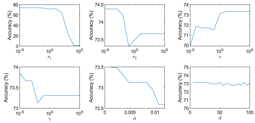
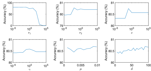
Refer to caption
Figure A.2: The evaluation of hyperparameter on BinAlpha dataset.
Refer to caption
Figure A.3: The evaluation of hyperparameter on FLW-102 dataset (features extracted by ResNet34).

D.3 Objectives Visualization

Refer to caption
(a) The first epoch
Refer to caption
(b) The 25-th epoch (log-scaled axes)
Refer to caption
(c) The final epoch (log-scaled axes)
Figure A.4: Radar chart of the objectives of D-NPSVC++ and DTWSVN on Cifar-10. We plot the objective of each class in the first epoch, the 25-th epoch, and the final epoch.

To show that the proposed D-NPSVC++ achieves a better solution to the multi-objective optimization problem (3) than DTWSVN (Li & Yang, 2022), we plot the radar charts to illustrate their objectives of each class in Figure A.4. Both two methods compute the objective of l𝑙l-th class by

Jl=1n[yi=ls(fl(𝒙i))+cK1yild(fl(𝒙i))],subscript𝐽𝑙1𝑛delimited-[]subscriptsubscript𝑦𝑖𝑙subscript𝑠subscript𝑓𝑙subscript𝒙𝑖𝑐𝐾1subscriptsubscript𝑦𝑖𝑙subscript𝑑subscript𝑓𝑙subscript𝒙𝑖J_{l}=\frac{1}{n}\left[\sum_{y_{i}=l}\ell_{s}(f_{l}({\bm{x}}_{i}))+\frac{c}{K-1}\sum_{y_{i}\not=l}\ell_{d}(f_{l}({\bm{x}}_{i}))\right], (A.14)

where the two methods use the same loss functions. It can be observed that D-NPSVC++ always achieve lower objectives in all classes than DTWSVN, which suggests the supority of D-NPSVC++ over DTWSVN and the effectiveness of the proposed training strategy. To explain this phenomenon, we compare the optimization criterion of these two methods:

DTWSVN: min𝜽1Kl=1KJl,subscript𝜽1𝐾superscriptsubscript𝑙1𝐾subscript𝐽𝑙\displaystyle\min_{{\bm{\theta}}}\frac{1}{K}\sum_{l=1}^{K}J_{l}, (A.15)
D-NPSVC++: {𝜽 step:min𝜽l=1KτlJl𝝉 step:max𝝉Δl=1KτlJl,s.t.l=1Kτl𝒁Jl=𝟎,cases𝜽 step:subscript𝜽superscriptsubscript𝑙1𝐾subscript𝜏𝑙subscript𝐽𝑙𝝉 step:formulae-sequencesubscript𝝉Δsuperscriptsubscript𝑙1𝐾subscript𝜏𝑙subscript𝐽𝑙stsuperscriptsubscript𝑙1𝐾subscript𝜏𝑙subscriptsubscript𝒁subscript𝐽𝑙0\displaystyle\begin{cases}{\bm{\theta}}\text{ step:}&\min_{{\bm{\theta}}}\sum_{l=1}^{K}\tau_{l}J_{l}\\ {\bm{\tau}}\text{ step:}&\max_{{\bm{\tau}}\in\Delta}\sum_{l=1}^{K}\tau_{l}J_{l},~{}\mathrm{s.t.}~{}\sum_{l=1}^{K}\tau_{l}\nabla_{{\bm{Z}}_{{\mathcal{B}}}}J_{l}=\bm{0},\end{cases} (A.16)

DTWSVN uses uniform scaling methods to minimize multiple dependent objectives, and usually fails to achieve the optimal solution (Sener & Koltun, 2018). The reason is that it does not consider the relationship between different objectives. In contrast, the proposed D-NPSVC++ aims to achieve Pareto optimality, which implements the trade-off of different objectives. Thus, D-NPSVC++ can obtain a better solution than DTWSVN.