A Bias–Variance Decomposition for Ensembles over Multiple Synthetic Datasets

Abstract

Recent studies have highlighted the benefits of generating multiple synthetic datasets for supervised learning, from increased accuracy to more effective model selection and uncertainty estimation. These benefits have clear empirical support, but the theoretical understanding of them is currently very light. We seek to increase the theoretical understanding by deriving bias-variance decompositions for several settings of using multiple synthetic datasets. Our theory predicts multiple synthetic datasets to be especially beneficial for high-variance downstream predictors, and yields a simple rule of thumb to select the appropriate number of synthetic datasets in the case of mean-squared error and Brier score. We investigate how our theory works in practice by evaluating the performance of an ensemble over many synthetic datasets for several real datasets and downstream predictors. The results follow our theory, showing that our insights are also practically relevant.

1 Introduction

Synthetic data has recently attracted significant attention for several application in machine learning. The idea is to generate a dataset that preserves the population-level attributes of the real data, making the synthetic data useful for analysis, while also accomplishing a secondary task, such as improving model evaluation (van Breugel et al., 2023b), fairness (van Breugel et al., 2021), data augmentation (Antoniou et al., 2018; Das et al., 2022) or privacy (Liew et al., 1985; Rubin, 1993). For the last application, differential privacy (DP) (Dwork et al., 2006) is often combined with synthetic data generation (Hardt et al., 2012; McKenna et al., 2021) to achieve provable privacy protection, since releasing synthetic data without DP can be vulnerable to membership inference attacks (van Breugel et al., 2023c; Meeus et al., 2023).

Several lines of work have considered generating multiple synthetic datasets from one real dataset for various purposes, including statistical inference (Rubin, 1993; Raghunathan et al., 2003; Räisä et al., 2023a) and supervised learning (van Breugel et al., 2023a). We focus on the latter setting.

In supervised learning, van Breugel et al. (2023a) proposed using multiple synthetic datasets in the form of an ensemble. They propose training a predictive model separately on each synthetic dataset, and ensembling these models by averaging their predictions, which they call a deep generative ensemble (DGE). We drop the word “deep” in this paper and use the term generative ensemble, as we do not require the generator to be deep in any sense. The DGE was empirically demonstrated to be beneficial in several ways by van Breugel et al. (2023a), including predictive accuracy, model evaluation, model selection, and uncertainty estimation. Followup work has applied DGEs to improve model evaluation under distribution shifts and for small subgroups (van Breugel et al., 2023b).

However, van Breugel et al. (2023a) have very little theoretical analysis of the generative ensemble. They justify the ensemble by assuming the synthetic data is generated from a posterior predictive distribution. This assumption can be justified heuristically for deep generative models through a Bayesian interpretation of deep ensembles (Lakshminarayanan et al., 2017; Wilson and Izmailov, 2020; Wilson, 2021). However this justification only applies to generators with highly multi-modal losses, like neural networks. It also does not provide any insight on how different choices in the setup, like the choice of downstream predictor, affect the performance of the ensemble.

The bias-variance decomposition (Geman et al., 1992) and its generalisations (Ueda and Nakano, 1996; Wood et al., 2023) are classical tools that provide insight into supervised learning problems. The standard bias-variance decomposition from Geman et al. (1992) considers predicting $y\in\mathbb{R}$ given features $x\in\mathcal{X}$, using predictor $g(x;D)$ that receives training data $D$. The mean-squared error (MSE) of $g$ can be decomposed into bias, variance, and noise terms:

$$\underbrace{\operatorname*{\mathbb{E}}_{D,y}[(y-g)^{2}]}_{\mathrm{MSE}}=\underbrace{(f(x)-\operatorname*{\mathbb{E}}_{D}[g])^{2}}_{\mathrm{Bias}}+\underbrace{\operatorname*{Var}_{D}[g]}_{\mathrm{Variance}}+\underbrace{\operatorname*{Var}_{y}[y]}_{\mathrm{Noise}}$$ (1)

where we have shortened $g=g(x;D)$ and $f(x)=\operatorname*{\mathbb{E}}_{y}[y]$. $x$ is considered fixed, so all the random quantities in the decomposition are implicitly conditioned on $x$. While MSE is typically only used with regression problems, the decomposition also applies to the Brier score (Brier, 1950) in classification, which is simply the MSE of class probabilities.

We seek to provide deeper theoretical understanding of generative ensembles through bias-variance decompositions, which provide a more fine-grained view of how different choices in the setup affect the end result.

Contributions

1. We derive a bias-variance decomposition for the MSE or Brier score of generative ensembles in Theorem 2.2. This decomposition is simply a sum of interpretable terms, which makes it possible to predict how various choices affect the error. In particular, the number of synthetic datasets only affects the variance-related terms in the decomposition, predicting that generative ensembles work best with high-variance and low bias models, like interpolating decision trees.

2. We derive a simple rule of thumb from our decomposition to select the number of synthetic datasets in Section 2.3. In summary, 2 synthetic datasets give 50% of the potential benefit from multiple synthetic datasets, 10 give 90% of the benefit and 100 give 99% of the benefit. This also applies to bagging ensembles like random forests, which is likely to be of independent interest.

3. We generalise the decomposition of Theorem 2.2 to differentially private (DP) generation algorithms that do not split their privacy budget between the multiple synthetic datasets in Theorem 2.4.

4. We evaluate the performance of a generative ensemble on several datasets, downstream prediction algorithms, and error metrics in Section 3. The results show that out theory applies in practice: multiple synthetic datasets generally decrease all of the error metrics, especially for high-variance models where the theory predicts multiple synthetic datasets to have the highest impact. In addition, our rule of thumb makes accurate predictions when the error can be accurately estimated.

1.1 Related Work

Ensembling generative models has been independently proposed several times (Wang et al., 2016; Choi et al., 2019; Luzi et al., 2020; Chen et al., 2023; van Breugel et al., 2023a). The inspiration of our work comes from van Breugel et al. (2023a), who proposed ensembling predictive models over multiple synthetic datasets, and empirically studied how this improves several aspects of performance in classification.

Generating multiple synthetic datasets has also been proposed with statistical inference in mind, for both frequentist (Rubin, 1993; Raghunathan et al., 2003; Räisä et al., 2023b), and recently Bayesian (Räisä et al., 2023a) inference. These works use the multiple synthetic datasets to correct statistical inferences for the extra uncertainty from synthetic data generation.

The bias-variance decomposition was originally derived by Geman et al. (1992) for standard regressors using MSE as the loss. James (2003) generalised the decomposition to symmetric losses, and Pfau (2013) generalised it to Bregman divergences.

Ueda and Nakano (1996) were the first to study the MSE bias-variance decomposition with ensembles, and Gupta et al. (2022); Wood et al. (2023) later extended the ensemble decomposition to other losses. All of these also apply to generative ensembles, but they only provide limited insight for them, as they do not separate the synthetic data generation-related terms from the downstream-related terms.

2 Bias-Variance Decompositions for Generative Ensembles

In this section, we make our main theoretical contributions. We start by defining our setting in Section 2.1. Then we derive a bias-variance decomposition for generative ensembles in Section 2.2 and derive a simple rule of thumb that can be used to select the number of synthetic datasets in Section 2.3. The generative ensemble decomposition doesn’t apply to several differentially private synthetic data generation methods that generate all synthetic datasets conditional on a single privatised value, so we generalise the decomposition to apply to those in Section 2.4. We also present a third decomposition that applies to Bregman divergences in Appendix B.

2.1 Problem Setting

We consider multiple synthetic datasets $D_{s}^{1:m}$, each of which is used to train an instance of a predictive model $g$. These models are combined into an ensemble $\hat{g}$ by averaging, so

$$\hat{g}(x;D_{s}^{1:m})=\frac{1}{m}\sum_{i=1}^{m}g(x;D_{s}^{i}).$$ (2)

We allow $g$ to be random, so $g$ can for example internally select among several predictive models to use randomly.

We assume the synthetic datasets are generated by first i.i.d. sampling parameters $\theta_{1:m}|D_{r}$ given the real data, and then sampling synthetic datasets $D_{s}^{i}\sim p(D_{s}|\theta_{i})$ given the parameters. This is how synthetic datasets are sampled in DGE (van Breugel et al., 2023a), where $\theta_{i}$ are the parameters of the generative neural network from independent training runs. This also encompasses bootstrapping, where $\theta_{i}$ would be the real dataset, and $p(D_{s}|\theta_{i})$ is the bootstrapping.

We will also consider a more general setting that applies to some differentially private synthetic data generators that do not fit into this setting in Section 2.4.

2.2 Mean-squared Error Decomposition

[] Let generator parameters $\theta_{1:m}$ be i.i.d. given the real data $D_{r}$, let the synthetic datasets be $D_{s}^{i}\sim p(D_{s}|\theta_{i})$ independently, and let $\hat{g}(x;D_{s}^{1:m})=\frac{1}{m}\sum_{i=1}^{m}g(x;D_{s}^{i})$. Then the mean-squared error in predicting $y$ from $x$ decomposes into six terms: model variance (MV), synthetic data variance (SDV), real data variance (RDV), synthetic data bias (SDB), model bias (MB), and noise $\operatorname*{Var}_{y}[y]$:

$$\mathrm{MSE}=\frac{1}{m}\mathrm{MV}+\frac{1}{m}\mathrm{SDV}+\mathrm{RDV}+(\mathrm{SDB}+\mathrm{MB})^{2}+\operatorname*{Var}_{y}[y],$$ (3)

where

$$\mathrm{MSE} =\operatorname*{\mathbb{E}}_{y,D_{r},D_{s}^{1:m}}[(y-\hat{g}(x;D_{s}^{1:m}))^{2}]$$ (4)

$$\mathrm{MV} =\operatorname*{\mathbb{E}}_{D_{r},\theta}\operatorname*{Var}_{D_{s}|\theta}[g(x;D_{s})]$$ (5)

$$\mathrm{SDV} =\operatorname*{\mathbb{E}}_{D_{r}}\operatorname*{Var}_{\theta|D_{r}}\operatorname*{\mathbb{E}}_{D_{s}|\theta}[g(x;D_{s})]$$ (6)

$$\mathrm{RDV} =\operatorname*{Var}_{D_{r}}\operatorname*{\mathbb{E}}_{D_{s}|D_{r}}[g(x;D_{s})]$$ (7)

$$\mathrm{SDB} =\operatorname*{\mathbb{E}}_{D_{r}}[f(x)-\operatorname*{\mathbb{E}}_{\theta|D_{r}}[f_{\theta}(x)]]$$ (8)

$$\mathrm{MB} =\operatorname*{\mathbb{E}}_{D_{r},\theta}[f_{\theta}(x)-\operatorname*{\mathbb{E}}_{D_{s}|\theta}[g(x;D_{s})]].$$ (9)

$f(x)=\operatorname*{\mathbb{E}}_{y}[y]$ is the optimal predictor for real data, $\theta$ is a single sample from the distribution of $\theta_{i}$, $D_{s}\sim p(D_{s}|\theta)$ is a single sample of the synthetic data generating process, and $f_{\theta}$ is the optimal predictor for the synthetic data generating process given parameters $\theta$. All random quantities are implicitly conditioned on $x$. The proofs of all theorems are in Appendix A.

We can immediately make actionable observations:

1. Increasing the number of synthetic datasets $m$ reduces the impact of MV and SDV. This means that high-variance models, like interpolating decision trees or 1-nearest neighbours, benefit the most from multiple synthetic datasets. These models should be favoured over low variance high bias models, even if the latter were better on the real data.

2. There is a simple rule-of-thumb on how many synthetic datasets are beneficial: $m$ synthetic datasets give a $1-\frac{1}{m}$ fraction of the possible benefit from multiple synthetic datasets. For example, $m=2$ gives 50% of the benefit, $m=10$ gives 90% and $m=100$ gives 99%. This rule-of-thumb can be used to predict the MSE with many synthetic datasets from the results on just two synthetic datasets. More details in Section 2.3.

We can also consider two extreme scenarios:

1. Generator is fitted perfectly, and generates from the real data generating distribution. Now

   $$\mathrm{MV} =\operatorname*{Var}_{D_{r}}[g(x;D_{r})]$$ (10)

   $$\mathrm{SDV} =0$$ (11)

   $$\mathrm{RDV} =0$$ (12)

   $$\mathrm{SDB} =0$$ (13)

   $$\mathrm{MB} =\operatorname*{\mathbb{E}}_{D_{r}}[f(x)-g(x;D_{r})]$$ (14)

   With one synthetic dataset, the result is the standard bias-variance trade-off. With multiple synthetic datasets, the impact of MV can be reduced, reducing the error compared to just using real data.

2. Return the real data: $D_{s}|D_{r}=D_{r}$ deterministically.

   $$\mathrm{MV} =0$$ (15)

   $$\mathrm{SDV} =0$$ (16)

   $$\mathrm{RDV} =\operatorname*{Var}_{D_{r}}[g(x;D_{r})]$$ (17)

   $$\mathrm{SDB} =0$$ (18)

   $$\mathrm{MB} =\operatorname*{\mathbb{E}}_{D_{r}}[f(x)-g(x;D_{r})]$$ (19)

   The result is the standard bias-variance trade-off. The number of synthetic datasets does not matter, as all of them would be the same anyway.

While both of these scenarios are unrealistic, they may be approximated by a well-performing algorithm. A generator that is a good approximation to either scenario could be considered to generate high-quality synthetic data. Multiple synthetic datasets are only beneficial in the first scenario, which shows that the synthetic data generation algorithm should have similar randomness to the real data generating process, and not just return a dataset that is close the the real one with little randomness.

2.3 Estimating the effect of Multiple Synthetic Datasets

Next, we consider estimating the variance terms MV and SDV in Theorem 2.2 from a small number of synthetic datasets and a test set. These estimates can then be used to asses if more synthetic datasets should be generated, and how many more are useful.

We can simplify Theorem 2.2 to

$$\mathrm{MSE}=\frac{1}{m}\mathrm{MV}+\frac{1}{m}\mathrm{SDV}+\mathrm{Others},$$ (20)

where Others does not depend on the number of synthetic datasets $m$. The usefulness of more synthetic datasets clearly depends on the magnitude of $\mathrm{MV}+\mathrm{SDV}$ compared to Others.

Since MSE depends on $m$, we can add a subscript to denote the $m$ in question: $\mathrm{MSE}_{m}$. Now (20) gives

$$\mathrm{MSE}_{m}=\mathrm{MSE}_{1}-\left(1-\frac{1}{m}\right)(\mathrm{MV}+\mathrm{SDV}).$$ (21)

If we have two synthetic datasets, we can estimate $\mathrm{MV}+\mathrm{SDV}$:

$$\begin{split}\mathrm{MV}+\mathrm{SDV}=2(\mathrm{MSE}_{1}-\mathrm{MSE}_{2}).\end{split}$$ (22)

If we have more than two synthetic datasets, we can set $x_{m}=1-\frac{1}{m}$ and $y_{m}=\mathrm{MSE}_{m}$ in (21):

$$y_{m}=y_{1}+x_{m}(\mathrm{MV}+\mathrm{SDV}),$$ (23)

so we can estimate $\mathrm{MV}+\mathrm{SDV}$ from linear regression on $(x_{m},y_{m})$. However, this will likely have a limited effect on the accuracy of the $\mathrm{MSE}_{m}$ estimates, as it will not reduce the noise in estimating $\mathrm{MSE}_{1}$, which has a significant effect in (21).

All terms in (20)-(23) depend on the target features $x$. We would like our estimates to be useful for typical $x$, so we will actually want to estimate $\operatorname*{\mathbb{E}}_{x}(\mathrm{MSE}_{m})$. Equations (20)-(23) remain valid if we take the expectation over $x$, so we can simply replace the MSE terms with their estimates that are computed from a test set.

Computing the estimates in practice will require that the privacy risk of publishing the test MSE is considered acceptable. The MSE for the estimate can also be computed from a separate validation set to avoid overfitting to the test set, but the risk of overfitting is small in this case, as $m$ has a monotonic effect on the MSE. Both of these caveats can be avoided by choosing $m$ using the rule of thumb that $m$ synthetic datasets give a $1-\frac{1}{m}$ of the potential benefit of multiple synthetic datasets, which is a consequence of (21).

Note that this MSE estimator can be applied to bagging ensembles (Breiman, 1996) like random forests (Breiman, 2001), since bootstrapping is a very simple form of synthetic data generation.

2.4 Differentially Private Synthetic Data Generators

Generating and releasing multiple synthetic datasets could increase the associated disclosure risk. One solution to this is differential privacy (DP) (Dwork et al., 2006; Dwork and Roth, 2014), which is a property of an algorithm that formally bounds to privacy leakage that can result from releasing the output of that algorithm. DP gives a quantitative upper bound on the privacy leakage, which is known as the privacy budget. Achieving DP requires adding extra noise to some point in the algorithm, lowering the utility of the result.

If the synthetic data is to be generated with DP, there are two possible ways to handle the required noise addition. The first is splitting the privacy budget across the $m$ synthetic datasets, and run the DP generation algorithm separately $m$ times. Theorem 2.2 applies in this setting. However, it is not clear if multiple synthetic datasets are beneficial in this case, as splitting the privacy budget requires adding more noise to each synthetic dataset. This also means that the rule of thumb from Section 2.3 will not apply. Most DP synthetic data generation algorithm would fall into this category (Aydore et al., 2021; Chen et al., 2020; Harder et al., 2021; Hardt et al., 2012; Liu et al., 2021; McKenna et al., 2019, 2021) if used to generate multiple synthetic datasets.

The second possibility is generating all synthetic datasets based on a single application of a DP mechanism. Specifically, a noisy summary $\tilde{s}$ of the real data is released under DP. The parameters $\theta_{1:m}$ are then sampled i.i.d. conditional on $\tilde{s}$, and the synthetic datasets are sampled conditionally on the $\theta_{1:m}$. This setting includes algorithms that release a posterior distribution under DP, and use the posterior to generate synthetic data, like the NAPSU-MQ algorithm (Räisä et al., 2023b) and DP variational inference (DPVI) (Jälkö et al., 2017, 2021).

The synthetic datasets are not i.i.d. given the real data in the second setting, so the setting described in Section 2.1 and assumed in Theorem 2.2 does not apply. However, the synthetic datasets are i.i.d. given the noisy summary $\tilde{s}$, so we obtain a similar decomposition as before. [] Let generator parameters $\theta_{1:m}$ be i.i.d. given a DP summary $\tilde{s}$ of the real data $D_{r}$, let the synthetic datasets be $D_{s}^{i}\sim p(D_{s}|\theta_{i})$ independently, and let $\hat{g}(x;D_{s}^{1:m})=\frac{1}{m}\sum_{i=1}^{m}g(x;D_{s}^{i})$. Then

$$\begin{split}\mathrm{MSE}&=\frac{1}{m}\mathrm{MV}+\frac{1}{m}\mathrm{SDV}+\mathrm{RDV}+\mathrm{DPVAR}\\ &+\,(\mathrm{SDB}+\mathrm{MB})^{2}+\operatorname*{Var}_{y}[y],\end{split}$$ (24)

where

$$\mathrm{MSE} =\operatorname*{\mathbb{E}}_{y,D_{r},\tilde{s},D_{s}^{1:m}}[(y-\hat{g}(x;D_{s}^{1:m}))^{2}]$$ (25)

$$\mathrm{MV} =\operatorname*{\mathbb{E}}_{D_{r},\tilde{s},\theta}\operatorname*{Var}_{D_{s}|\theta}[g(x;D_{s})]$$ (26)

$$\mathrm{SDV} =\operatorname*{\mathbb{E}}_{D_{r},\tilde{s}}\operatorname*{Var}_{\theta|\tilde{s}}\operatorname*{\mathbb{E}}_{D_{s}|\theta}[g(x;D_{s})]$$ (27)

$$\mathrm{RDV} =\operatorname*{Var}_{D_{r}}\operatorname*{\mathbb{E}}_{D_{s}|D_{r}}[g(x;D_{s})]$$ (28)

$$\mathrm{DPVAR} =\operatorname*{\mathbb{E}}_{D_{r}}\operatorname*{Var}_{\tilde{s}|D_{r}}\operatorname*{\mathbb{E}}_{D_{s}|\tilde{s}}[g(x;D_{s})]$$ (29)

$$\mathrm{SDB} =\operatorname*{\mathbb{E}}_{D_{r},\tilde{s}}[f(x)-\operatorname*{\mathbb{E}}_{\theta|\tilde{s}}[f_{\theta}(x)]]$$ (30)

$$\mathrm{MB} =\operatorname*{\mathbb{E}}_{D_{r},\tilde{s},\theta}[f_{\theta}(x)-\operatorname*{\mathbb{E}}_{D_{s}|\theta}[g(x;D_{s})]].$$ (31)

$f(x)=\operatorname*{\mathbb{E}}_{y}[y]$ is the optimal predictor for real data, $\theta$ is a single sample from the distribution of $\theta_{i}$, $D_{s}\sim p(D_{s}|\theta)$ is a single sample of the synthetic data generating process, and $f_{\theta}$ is the optimal predictor for the synthetic data generating process given parameters $\theta$. All random quantities are implicitly conditioned on $x$.

The takeaways from Theorem 2.4 are mostly the same as from Theorem 2.2, and the estimator from Section 2.3 also applies. The main difference is the DPVAR term in Theorem 2.4, which accounts for the added DP noise. As expected, the impact of DPVAR cannot be reduced with additional synthetic datasets.

3 Experiments

Figure 1: Comparison of synthetic data generation algorithms for several prediction algorithms on the California housing dataset, with 1 to 10 synthetic datasets. DDPM and synthpop achieve smaller MSE in the downstream predictions, so they were selected for further experiments. SP-P and SP-IP are the proper and improper variants of synthpop, and DDPM-KL is DDPM with KL divergence loss. 1-NN and 5-NN are nearest neighbours with 1 and 5 neighbours. The dashed black lines show the performance of each prediction algorithm on the real data, and the solid black line shows the performance of the best predictor, random forest, on the real data. The results are averaged over 3 repeats, with different train-test splits. The error bars are 95% confidence intervals formed by bootstrapping over the repeats. Linear regression was omitted, as it had nearly identical results as ridge regression. Table 3 in the Appendix contains the numbers in the plots, including ridge regression.

In this section, we describe our experiments. The common theme in all of them is generating synthetic data and evaluating the performance of several downstream prediction algorithms trained on the synthetic data. The performance evaluation uses a test set of real data, which is split from the whole dataset before generating synthetic data.

The downstream algorithms we consider are nearest neighbours with 1 or 5 neighbours (1-NN and 5-NN), decision tree (DT), random forest (RF), gradient boosted trees (GB), a multilayer perceptron (MLP) and a support vector machine (SVM) for both classification and regression. We also use linear regression (LR) and ridge regression (RR) on regression tasks, and logistic regression (LogR) on classification tasks, though we omit linear regression from the main text plots, as its results are nearly identical to ridge regression. Decision trees and 1-NN have a very high variance, as both interpolate the training data with the hyperparameters we use. Linear, ridge, and logistic regression have fairly small variance in contrast. Appendix C contains more details on the experimental setup, including details on the datasets, and downstream algorithm hyperparameters.

3.1 Synthetic Data Generation Algorithms

First, we compare several synthetic data generation algorithms to see which algorithms are most interesting for subsequent experiments. We use the California housing dataset, where the downstream task is regression. The algorithms we compare are DDPM (Kotelnikov et al., 2023), TVAE (Xu et al., 2019), CTGAN (Xu et al., 2019) and synthpop (Nowok et al., 2016). DDPM, TVAE and CTGAN are a diffusion model, a variational autoencoder and a GAN that are designed for tabular data. We use the implementations from the synthcity library for these. Synthpop generates synthetic data by sampling one column from the real data, and generating the other columns by sequentially training a predictive model on the real data, and predicting the next column from the already generated ones. We use the implementation from the authors (Nowok et al., 2016).

We use the default hyperparameters for all of the algorithms. Synthpop and DDPM have a setting that could potentially affect the randomness in the synthetic data generation, so we include both possibilities for these settings in this experiment. For synthpop, this setting is whether the synthetic data is generated from a Bayesian posterior predictive distribution, which synthpop calls “proper” synthetic data. For DDPM, this setting is whether the loss function is MSE or KL divergence. In the plots, the two variants of synthpop are called “SP-P” and “SP-IP” for the proper and improper variants, and the variants of DDPM are “DDPM” and “DDPM-KL”.

(a) Abalone

(b) ACS 2018

(c) California Housing

(d) Insurance

Figure 2: MSE of the ensemble of downstream predictors on the regression datasets, with varying number of synthetic datasets $m$ from either DDPM or synthpop (SP-P). Increasing the number of synthetic datasets generally decreases MSE, especially for decision trees and 1-NN. The predictors are nearest neighbours with 1 or 5 neighbours (1-NN and 5-NN), decision tree (DT), random forest (RF), a multilayer perceptron (MLP), gradient boosted trees (GB), a support vector machine (SVM) and ridge regression (RR). The black line is the MSE of the best predictor on real data. The results are averaged over 3 repeats. The error bars are 95% confidence intervals formed by bootstrapping over the repeats. We omitted linear regression from the plot, as it had almost identical results to ridge regression. Tables 4 to 7 in the Appendix contain the numbers from the plots, including ridge regression.

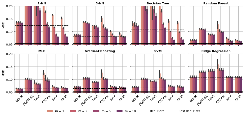
The results of the comparison are shown in Figure 1. We see that synthpop and DDPM with MSE loss generally outperform the other generation algorithms, so we select them for the subsequent experiments. There is very little difference between the two variants of synthpop, so we choose the “proper” variant due to its connection with the Bayesian reasoning for using multiple synthetic datasets.

3.2 Main Experiment

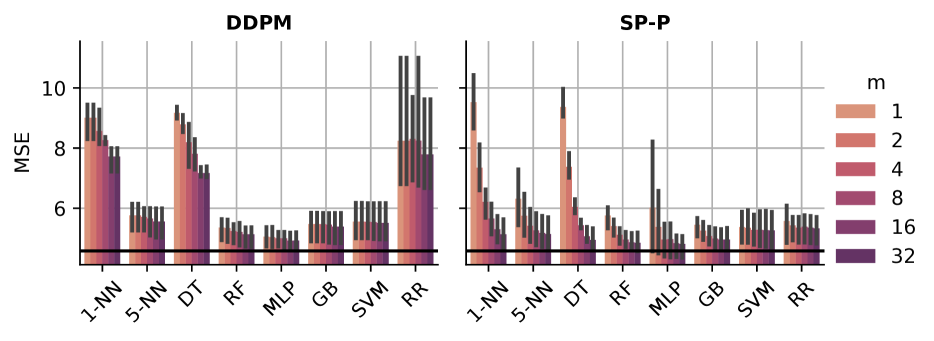
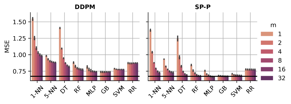
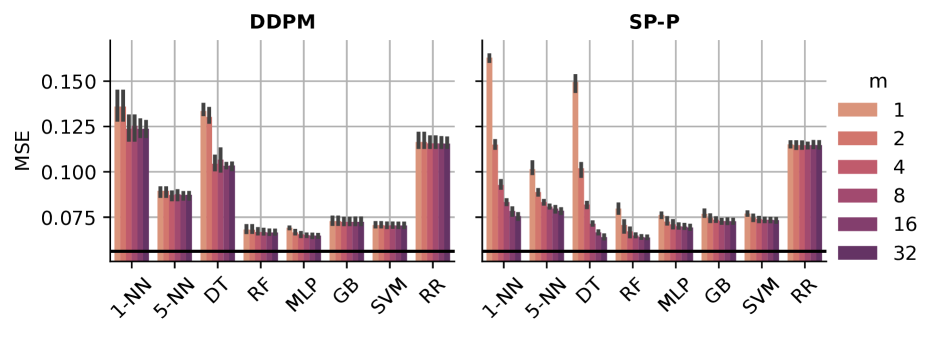
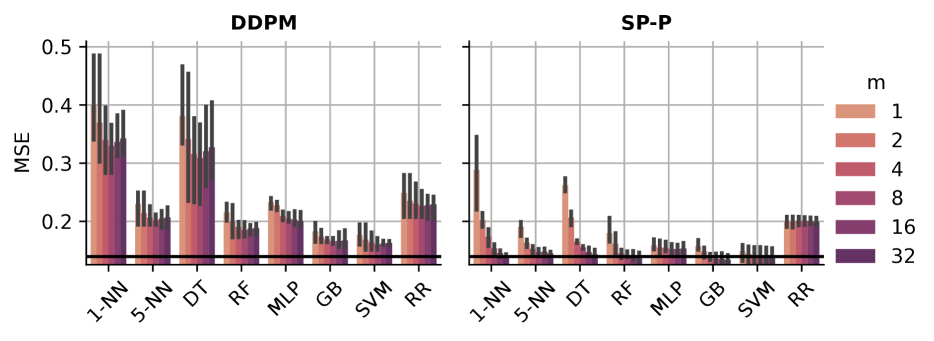
As our main experiment, we evaluate the performance of the synthetic data ensemble on 7 datasets, containing 4 regression and 3 classification tasks. See Appendix C.1 for details on the datasets. We use both DDPM and synthpop as the synthetic data generator, and generate 32 synthetic datasets, of which between 1 and 32 are used to train the ensemble. The results are averaged over 3 runs with different train-test splits.

On the regression datasets, our error metric is MSE, which is the subject of Theorem 2.2. The results in Figure 2 show that a larger number of synthetic datasets generally decreases MSE. The decrease is especially clear with synthpop and downstream algorithms that have a high variance like decision trees and 1-NN. Low-variance algorithms like ridge regression have very little if any decrease from multiple synthetic datasets. This is consistent with Theorem 2.2, where the number of synthetic datasets only affects the variance-related terms.

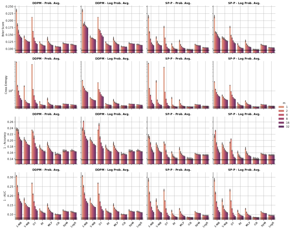
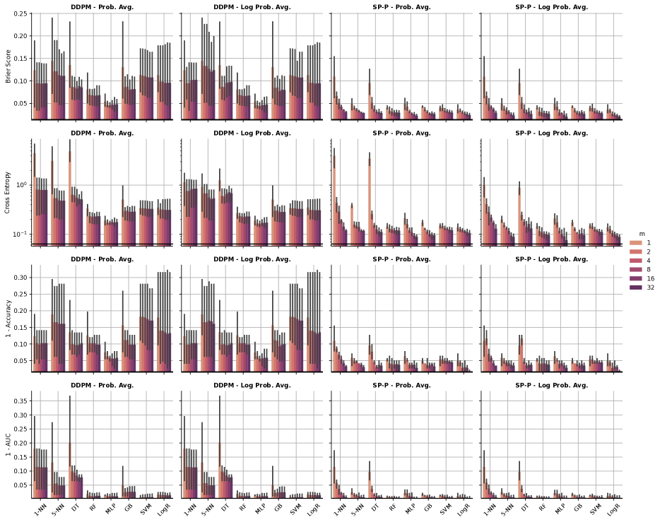
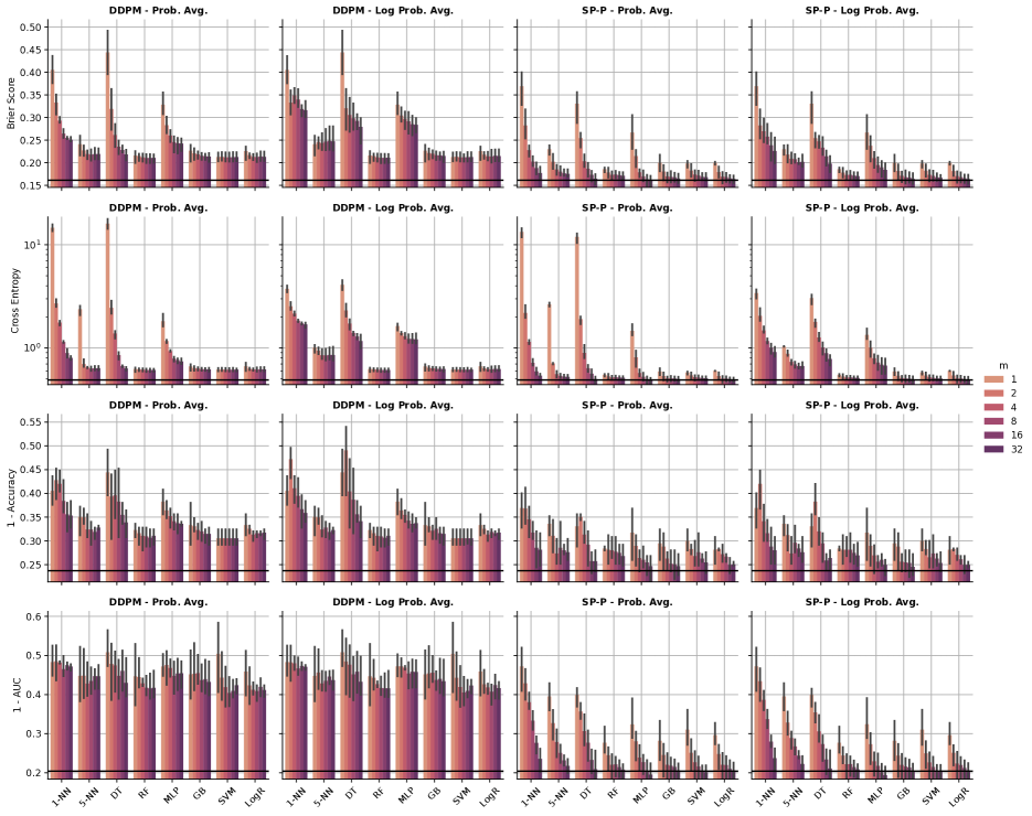
On the classification datasets, we consider 4 error metrics. Brier score (Brier, 1950) is MSE of the class probability predictions, so Theorem 2.2 applies to it. Cross entropy is a Bregman divergence, so Theorem B.2 from Appendix B applies to it. We also included accuracy and area under the ROC curve (AUC) even though our theory does not apply to them, as they are common and interpretable error metrics, so it is interesting to see how multiple synthetic datasets affect them. We use their complements in the plots, so that lower is better for all plotted metrics. We only present the Brier score results in the main text in Figure 3, and defer the rest to Figures 5, 6 and 7 in Appendix D.

(a) Adult

(b) Breast Cancer

(c) German Credit

Figure 3: Brier score of the ensemble of downstream predictors with varying numbers of synthetic datasets $m$, generated by either DDPM and synthpop, and averaging either probabilities or log probabilities, on the classification datasets. Increasing the number of synthetic datasets generally decreases the score, except in cases where one synthetic dataset is already enough to meet the real data performance. Probability averaging is generally outperforming log probability averaging. The predictors are logistic regression nearest neighbours with 1 or 5 neighbours (1-NN and 5-NN), decision tree (DT), random forest (RF), a multilayer perceptron (MLP), gradient boosted trees (GB), a support vector machine (SVM) and logistic regression (LogR). The black line show the loss of the best downstream predictor trained on real data. The results are averaged over 3 repeats with different train-test splits. The error bars are 95% confidence intervals formed by bootstrapping over the repeats. Tables 8 to 10 in the Appendix contain the numbers from the plots.

Because Theorem B.2 only applies to cross entropy when averaging log probabilities instead of probabilities, we compare both ways of averaging.

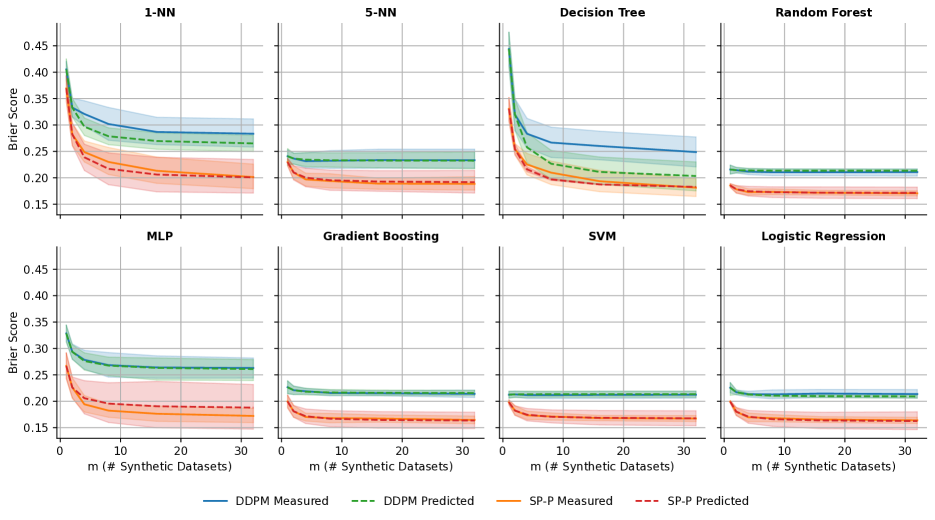
The results on the classification datasets in Figure 3 are similar to the regression experiment. A larger number of synthetic datasets generally decreases the score, especially for the high-variance models. Logistic regression is an exception, as it has low variance, as are algorithms that match the performance on the real data already with one synthetic dataset.

Probability averaging generally outperforms log probability averaging on Brier score and cross entropy. There is very little difference between the two on accuracy and AUC, which suggests that probability averaging is generally better than log-probability averaging.

In Appendix D.1, we estimate the MV and SDV terms of the decomposition in Theorem 2.2. These confirm our claims on the model variances: decision trees and 1-NN have a high variance, while linear, ridge and logistic regression have a low variance.

3.3 Predicting MSE from Two Synthetic Datasets

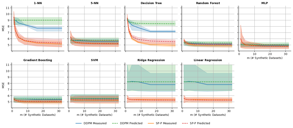
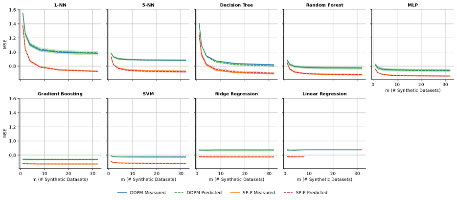
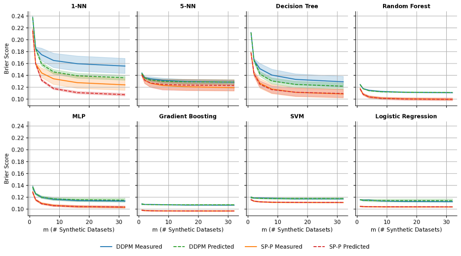
Next, we evaluate the predictions our rule of thumb from Section 2.3 makes. To recap, our rule of thumb predicts that the maximal benefit from multiple synthetic datasets is $2(\mathrm{MSE}_{1}-\mathrm{MSE}_{2})$, and $m$ synthetic datasets achieve a $1-\frac{1}{m}$ fraction of this benefit.

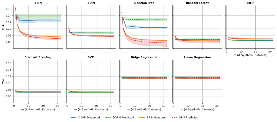
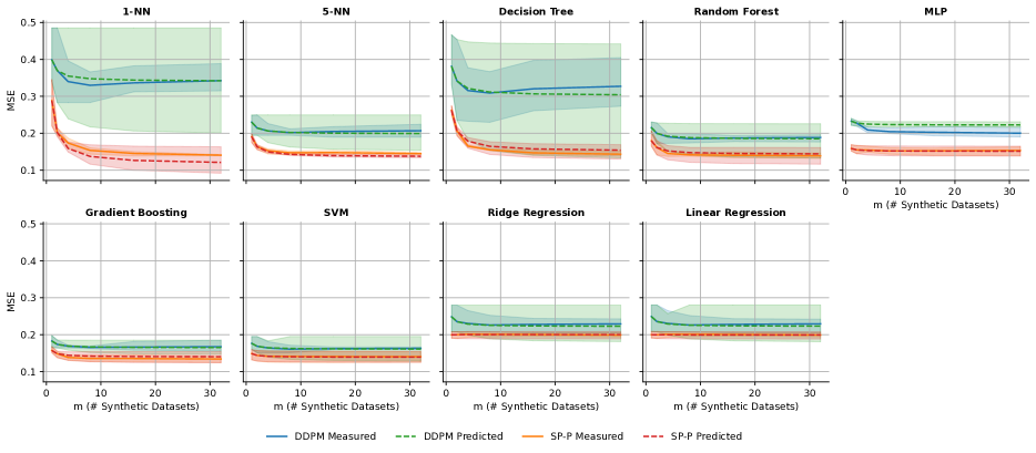
To evaluate the predictions from the rule, we estimate the MSE on regression tasks and Brier score on classification tasks for one and two synthetic datasets from the test set. The setup is otherwise identical to Section 3.2, and the train-test splits are the same. We plot the predictions from the rule, and compare them with the measured test errors with more than two synthetic datasets.

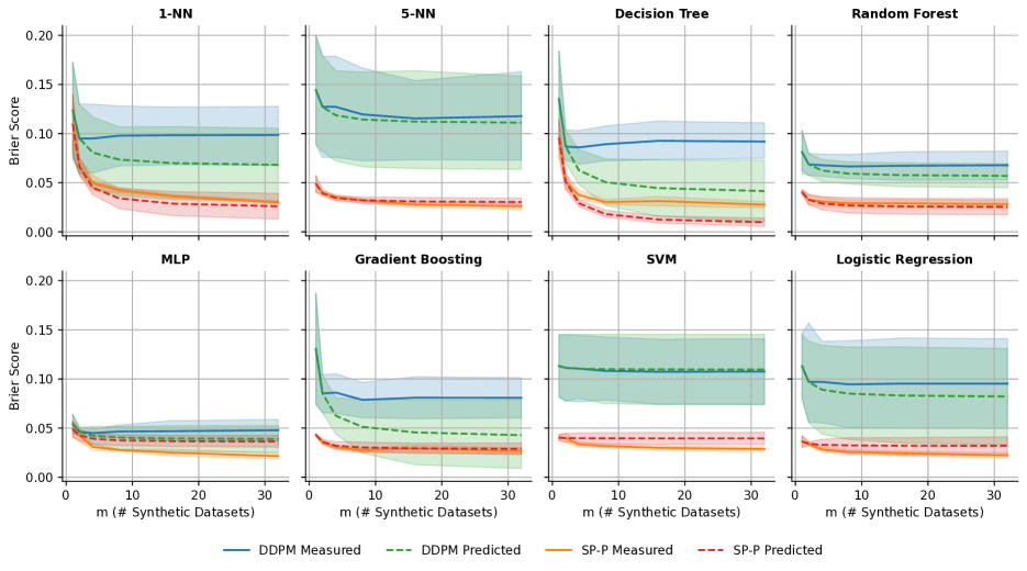
Figure 4 contains the results for the ACS 2018 dataset, and Figures 8 to 11 in the Appendix contain the results for the other datasets. The rule of thumb is very accurate on ACS 2018 and reasonably accurate on the other datasets. The variance of the prediction depends heavily on the variance of the errors computed from the test data.

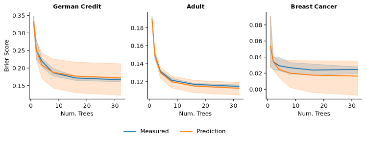
We also evaluated the rule on random forests without synthetic data, as it also applies to them. In this setting, the number of trees in the random forest is analogous to the number of synthetic datasets. We use the same datasets as in the previous experiments and use the same train-test splits of the real data. The results are in Figure 12 in the Appendix. The prediction is accurate when the test error is accurate, but can have high variance.

Figure 4: MSE prediction on the ACS 2018 dataset. The prediction is very accurate on this dataset. The solid lines for DDPM and synthpop (SP-P) show the same MSEs as Figure 2, while the dashed lines show predicted MSEs. 1-NN and 5-NN are nearest neighbours with 1 or 5 neighbours. We omitted downstream algorithms with uninteresting flat curves. See Figure 8 in the appendix for the full plot, and Figure 9 plots for the other datasets. Table 11 in the Appendix contains the numbers from the plots. The results are averaged over 3 repeats with different train-test splits. The error bands are 95% confidence intervals formed by bootstrapping over the repeats.

4 Discussion

Limitations

Our theory assumes that the synthetic datasets are generated i.i.d. given either the real data or a DP summary. This means our theory will not apply to more complicated schemes for generating multiple synthetic datasets, like excluding generators based on some criteria (Dikici et al., 2020) or collecting the generators from different points of a single training run (Wang et al., 2016). However, i.i.d. synthetic datasets are still very relevant, as they are the simplest case, and uncertainty estimation techniques for statistical inference with synthetic data (Raghunathan et al., 2003; Räisä et al., 2023a) require i.i.d. synthetic datasets.

Conclusion

We derived bias-variance decompositions for using synthetic data in several cases: for MSE or Brier score with i.i.d. synthetic datasets given the real data and MSE with i.i.d.  synthetic datasets given a DP summary of the real data. The decompositions make actionable predictions, such as yielding a simple rule of thumb that can be used to select the number of synthetic datasets. We empirically examined the performance of generative ensembles on several real datasets and downstream predictors, and found that the predictions of the theory generally hold in practice. These findings significantly increase the theoretical understanding of generative ensembles, which is very limited in prior literature.

Broader Impacts

Generating multiple synthetic datasets can potentially increase disclosure risk if appropriate precautions, such as differential privacy, are not used. Because of this, care should be taken and precautions like differential privacy should be used if possible when releasing multiple synthetic datasets of sensitive data, despite our theory suggesting that multiple synthetic datasets are beneficial for utility.

Appendix A Missing Proofs

See 2.2

Proof.

With $m$ synthetic datasets $D_{s}^{1:m}$ and model $\hat{g}(x,D_{s}^{1:m})$ that combines the synthetic datasets, the classical bias-variance decomposition gives

$$\operatorname*{\mathbb{E}}_{y,D_{r},D_{s}^{1:m}}[(y-\hat{g}(x;D_{s}^{1:m}))^{2}]=(f(x)-\operatorname*{\mathbb{E}}_{D_{r},D_{s}^{1:m}}[\hat{g}(x;D_{s}^{1:m})])^{2}+\operatorname*{Var}_{D_{r},D_{s}^{1:m}}[\hat{g}(x;D_{s}^{1:m})]+\operatorname*{Var}_{y}[y].$$ (32)

Using the independence of the synthetic datasets, these can be decomposed further:

$$\operatorname*{\mathbb{E}}_{D_{r},D_{s}^{1:m}}[\hat{g}(x;D_{s}^{1:m})]=\frac{1}{m}\operatorname*{\mathbb{E}}_{D_{r}}\operatorname*{\mathbb{E}}_{D_{s}^{1:m}|D_{r}}\left[\sum_{i=1}^{m}g(x,D_{s}^{i})\right]=\operatorname*{\mathbb{E}}_{D_{r}}\operatorname*{\mathbb{E}}_{D_{s}|D_{r}}[g(x,D_{s})]=\operatorname*{\mathbb{E}}_{D_{r},D_{s}}[g(x,D_{s})],$$ (33)

$$\begin{split}\operatorname*{Var}_{D_{r},D_{s}^{1:m}}[\hat{g}(x;D_{s}^{1:m})]&=\operatorname*{\mathbb{E}}_{D_{r}}\operatorname*{Var}_{D_{s}^{1:m}|D_{r}}\left[\frac{1}{m}\sum_{i=1}^{m}g(x;D_{s}^{i})\right]+\operatorname*{Var}_{D_{r}}\operatorname*{\mathbb{E}}_{D_{s}^{1:m}|D_{r}}\left[\frac{1}{m}\sum_{i=1}^{m}g(x;D_{s}^{i})\right]\\ &=\frac{1}{m^{2}}\operatorname*{\mathbb{E}}_{D_{r}}\operatorname*{Var}_{D_{s}^{1:m}|D_{r}}\left[\sum_{i=1}^{m}g(x;D_{s}^{i})\right]+\operatorname*{Var}_{D_{r}}\operatorname*{\mathbb{E}}_{D_{s}|D_{r}}\left[g(x;D_{s})\right]\\ &=\frac{1}{m}\operatorname*{\mathbb{E}}_{D_{r}}\operatorname*{Var}_{D_{s}|D_{r}}\left[g(x;D_{s})\right]+\operatorname*{Var}_{D_{r}}\operatorname*{\mathbb{E}}_{D_{s}|D_{r}}\left[g(x;D_{s})\right],\end{split}$$ (34)

and

$$\operatorname*{Var}_{D_{s}|D_{r}}[g(x;D_{s})]=\operatorname*{\mathbb{E}}_{\theta|D_{r}}\operatorname*{Var}_{D_{s}|\theta}[g(x;D_{s})]+\operatorname*{Var}_{\theta|D_{r}}\operatorname*{\mathbb{E}}_{D_{s}|\theta}[g(x,D_{s})].$$ (35)

The bias can be decomposed with $f_{\theta}(x)$:

$$\begin{split}f(x)-\operatorname*{\mathbb{E}}_{D_{r},D_{s}}[g(x;D_{s})]&=\operatorname*{\mathbb{E}}_{D_{r},\theta}[f(x)-f_{\theta}(x)+f_{\theta}(x)-\operatorname*{\mathbb{E}}_{D_{s}|\theta}[g(x;D_{s})]]\\ &=\operatorname*{\mathbb{E}}_{D_{r}}[f(x)-\operatorname*{\mathbb{E}}_{\theta|D_{r}}[f_{\theta}(x)]]+\operatorname*{\mathbb{E}}_{D_{r},\theta}[f_{\theta}(x)-\operatorname*{\mathbb{E}}_{D_{s}|\theta}[g(x;D_{s})]]\end{split}$$ (36)

Combining all of these gives the claim. ∎

See 2.4

Proof.

Using $\tilde{s}$ in place of the real data in Theorem 2.2 gives

$$\mathrm{MSE}=\frac{1}{m}\mathrm{MV}+\frac{1}{m}\mathrm{SDV}+\operatorname*{Var}_{D_{r},\tilde{s}}\operatorname*{\mathbb{E}}_{D_{s}|\tilde{s}}[g(x;D_{s})]+(\mathrm{SDB}+\mathrm{MB})^{2}+\operatorname*{Var}_{y}[y],$$ (37)

where

$$\mathrm{MSE} =\operatorname*{\mathbb{E}}_{y,D_{r},\tilde{s},D_{s}^{1:m}}[(y-\hat{g}(x;D_{s}^{1:m}))^{2}]$$ (38)

$$\mathrm{MV} =\operatorname*{\mathbb{E}}_{D_{r},\tilde{s},\theta}\operatorname*{Var}_{D_{s}|\theta}[g(x;D_{s})]$$ (39)

$$\mathrm{SDV} =\operatorname*{\mathbb{E}}_{D_{r},\tilde{s}}\operatorname*{Var}_{\theta|\tilde{s}}\operatorname*{\mathbb{E}}_{D_{s}|\theta}[g(x;D_{s})]$$ (40)

$$\mathrm{SDB} =\operatorname*{\mathbb{E}}_{D_{r},\tilde{s}}[f(x)-\operatorname*{\mathbb{E}}_{\theta|\tilde{s}}[f_{\theta}(x)]]$$ (41)

$$\mathrm{MB} =\operatorname*{\mathbb{E}}_{D_{r},\tilde{s},\theta}[f_{\theta}(x)-\operatorname*{\mathbb{E}}_{D_{s}|\theta}[g(x;D_{s})]].$$ (42)

We can additionally decompose

$$\begin{split}\operatorname*{Var}_{D_{r},\tilde{s}}\operatorname*{\mathbb{E}}_{D_{s}|\tilde{s}}[g(x;D_{s})]&=\operatorname*{\mathbb{E}}_{D_{r}}\operatorname*{Var}_{\tilde{s}|D_{r}}\operatorname*{\mathbb{E}}_{D_{s}|\tilde{s}}[g(x;D_{s})]+\operatorname*{Var}_{D_{r}}\operatorname*{\mathbb{E}}_{\tilde{s}|D_{r}}\operatorname*{\mathbb{E}}_{D_{s}|\tilde{s}}[g(x;D_{s})]\\ &=\operatorname*{\mathbb{E}}_{D_{r}}\operatorname*{Var}_{\tilde{s}|D_{r}}\operatorname*{\mathbb{E}}_{D_{s}|\tilde{s}}[g(x;D_{s})]+\operatorname*{Var}_{D_{r}}\operatorname*{\mathbb{E}}_{D_{s}|D_{r}}[g(x;D_{s})]\end{split}$$ (43)

This reveals the DP-related variance term

$$\mathrm{DPVAR}=\operatorname*{\mathbb{E}}_{D_{r}}\operatorname*{Var}_{\tilde{s}|D_{r}}\operatorname*{\mathbb{E}}_{D_{s}|\tilde{s}}[g(x;D_{s})]$$ (44)

so we have

$$\mathrm{MSE}=\frac{1}{m}\mathrm{MV}+\frac{1}{m}\mathrm{SDV}+\mathrm{RDV}+\mathrm{DPVAR}+(\mathrm{SDB}+\mathrm{MB})^{2}+\operatorname*{Var}_{y}[y].$$ (45)

∎

Appendix B Bias-Variance Decomposition for Bregman Divergences

B.1 Background: Bregman Divergences

A Bregman divergence (Bregman, 1967) $D_{F}\colon\mathbb{R}^{d}\times\mathbb{R}^{d}\to\mathbb{R}$ is a loss function

$$D_{F}(y,g)=F(y)-F(g)-\nabla F(g)^{T}(y-g)$$ (46)

where $F\colon\mathbb{R}^{d}\to\mathbb{R}$ is a strictly convex differentiable function. Many common error metrics, like MSE and cross entropy, can be expressed as expected values of a Bregman divergence. In fact, proper scoring rules can be characterised via Bregman divergences (Gneiting and Raftery, 2007; Kimpara et al., 2023). Table 1 shows how the metrics we consider are expressed as Bregman divergences (Gupta et al., 2022).

Pfau (2013) derive the following bias-variance decomposition for Bregman divergences:

$$\underbrace{\operatorname*{\mathbb{E}}[D(y,g)]}_{\mathrm{Error}}=\underbrace{\operatorname*{\mathbb{E}}[D(y,\operatorname*{\mathbb{E}}y)]}_{\mathrm{Noise}}+\underbrace{D(\operatorname*{\mathbb{E}}y,\mathcal{E}g)}_{\mathrm{Bias}}+\underbrace{\operatorname*{\mathbb{E}}D(\mathcal{E}g,g)}_{\mathrm{Variance}}$$ (47)

$y$ is the true value, and $g$ is the predicted value. All of the random quantities are conditioned on $x$. $\mathcal{E}$ is a central prediction:

$$\mathcal{E}g=\operatorname*{argmin}_{z}\operatorname*{\mathbb{E}}D(z,g).$$ (48)

The variance term can be used to define a generalisation of variance:

$$\mathcal{V}g=\operatorname*{\mathbb{E}}D(\mathcal{E}g,g)$$ (49)

$\mathcal{E}$ and $\mathcal{V}$ can also be defined conditionally on some random variable $Z$ by making the expectations conditional on $Z$ in the definitions. These obey generalised laws of total expectation and variance (Gupta et al., 2022):

$$\mathcal{E}g=\mathcal{E}_{Z}[\mathcal{E}_{g|Z}[g]]$$ (50)

and

$$\mathcal{V}g=\operatorname*{\mathbb{E}}_{Z}[\mathcal{V}_{g|Z}[g]]+\mathcal{V}_{Z}[\mathcal{E}_{g|Z}[g]].$$ (51)

The convex dual of $g$ is $g^{*}=\nabla F(g)$. The central prediction $\mathcal{E}g$ can also be expressed as an expectation over the convex dual (Gupta et al., 2022):

$$\mathcal{E}g=(\operatorname*{\mathbb{E}}g^{*})^{*}$$ (52)

Table 1: Common error metrics as Bregman divergences. $g$ denotes a prediction in regression and $p$ denotes predicted class probabilities in classification. $g^{(j)}$ and $p^{(j)}$ denote the predictions of different ensemble members. $y$ is the correct value in regression, and a one-hot encoding of the correct class in classification. The binary classification Brier score only looks at probabilities for one class. If the multiclass Brier score is used with two classes, it is twice the binary Brier score.

Error Metric	$D_{F}$	$F(t)$	Dual Average
MSE	$(y-g)^{2}$	$t^{2}$	$\frac{1}{m}\sum_{j=1}^{m}g^{(j)}$
Brier Score (2 classes)	$(y_{1}-p_{1})^{2}$	$t^{2}$	$\frac{1}{m}\sum_{j=1}^{m}p^{(j)}$
Brier Score (Multiclass)	$\sum_{i}(y_{i}-p_{i})^{2}$	$\sum_{i}t_{i}^{2}$	$\frac{1}{m}\sum_{j=1}^{m}p^{(j)}$
Cross Entropy	$-\sum_{i}y_{i}\ln p_{i}$	$\sum_{i}t_{i}\ln t_{i}$	$\mathrm{softmax}\left(\frac{1}{m}\sum_{j=1}^{m}\ln p^{(j)}\right)$

Gupta et al. (2022) study the bias-variance decomposition of Bregman divergence on a generic ensemble. They show that if the ensemble aggregates prediction by averaging them, bias is not preserved, and can increase. As a solution, they consider dual averaging, that is

$$\hat{g}=\left(\frac{1}{m}\sum_{i=1}^{m}g_{i}^{*}\right)^{*}$$ (53)

for models $g_{1},\dotsc,g_{m}$ forming the ensemble $\hat{g}$. They show that the bias is preserved in the dual averaged ensemble, and derive a bias-variance decomposition for them. For mean squared error, the dual average is simply the standard average, but for cross entropy, it corresponds to averaging log probabilities.

B.2 Bregman Divergence Decomposition for Synthetic Data

We extend the Bregman divergence decomposition for ensembles from Gupta et al. (2022) to generative ensembles. To prove Theorem B.2, we use the following lemma. [Gupta et al. 2022, Proposition 5.3] Let $X_{1},\dotsc,X_{m}$ be i.i.d.  random variables and let $\hat{X}=(\sum_{i=1}^{m}X_{i}^{*})^{*}$ be their dual average. Then $\mathcal{E}\hat{X}=\mathcal{E}X$, $\mathcal{V}\hat{X}\leq\mathcal{V}X$ and for any independent $Y$, $D(\operatorname*{\mathbb{E}}Y,\mathcal{E}\hat{X})=D(\operatorname*{\mathbb{E}}Y,\mathcal{E}X)$.

[] When the synthetic datasets $D_{s}^{1:m}$ are i.i.d.  given the real data $D_{r}$ and $\hat{g}(x;D_{s}^{1:m})=(\frac{1}{m}\sum_{i=1}^{m}g(x;D_{s}^{i})^{*})^{*}$,

$$\mathrm{Error}\leq\mathrm{MV}+\mathrm{SDV}+\mathrm{RDV}+\mathrm{Bias}+\mathrm{Noise}$$ (54)

where

$$\mathrm{Error} =\operatorname*{\mathbb{E}}_{y,D_{r},D_{s}^{1:m}}[D(y,\hat{g})]$$ (55)

$$\mathrm{MV} =\operatorname*{\mathbb{E}}_{D_{r}}\operatorname*{\mathbb{E}}_{\theta|D_{r}}\mathcal{V}_{D_{s}|\theta}[g]$$ (56)

$$\mathrm{SDV} =\operatorname*{\mathbb{E}}_{D_{r}}\mathcal{V}_{\theta|D_{r}}\mathcal{E}_{D_{s}|\theta}[g]$$ (57)

$$\mathrm{RDV} =\mathcal{V}_{D_{r}}\mathcal{E}_{D_{s}|D_{r}}[g]$$ (58)

$$\mathrm{Bias} =D\left(\operatorname*{\mathbb{E}}_{y}y,\mathcal{E}_{D_{r}}\mathcal{E}_{D_{s}|D_{r}}[g]\right)$$ (59)

$$\mathrm{Noise} =\operatorname*{\mathbb{E}}_{y}\left[D(y,\operatorname*{\mathbb{E}}_{y}y)\right]$$ (60)

Proof.

Plugging the ensemble $\hat{g}$ into the decomposition (47) gives

$$\operatorname*{\mathbb{E}}_{y,D_{r},D_{s}^{1:m}}[D(y,\hat{g})]=\operatorname*{\mathbb{E}}_{y}[D(y,\operatorname*{\mathbb{E}}_{y}y)]+D(\operatorname*{\mathbb{E}}_{y}y,\mathcal{E}_{D_{r},D_{s}^{1:m}}\hat{g})+\mathcal{V}_{D_{r},D_{s}^{1:m}}[\hat{g}]$$ (61)

Applying the generalised laws of expectation and variance, and Lemma B.2 to the variance term, we obtain:

$$\mathcal{V}_{D_{r},D_{s}^{1:m}}[\hat{g}] =\operatorname*{\mathbb{E}}_{D_{r}}\mathcal{V}_{D_{s}^{1:m}|D_{r}}[\hat{g}]+\mathcal{V}_{D_{r}}\mathcal{E}_{D_{s}^{1:m}|D_{r}}[\hat{g}]$$ (62)

For the second term on the right:

$$\mathcal{E}_{D_{s}^{1:m}|D_{r}}[\hat{g}]=\mathcal{E}_{D_{s}|D_{r}}[g],$$ (63)

which gives the RDV:

$$\mathcal{V}_{D_{r}}\mathcal{E}_{D_{s}^{1:m}|D_{r}}[\hat{g}]=\mathcal{V}_{D_{r}}\mathcal{E}_{D_{s}|D_{r}}[g].$$ (64)

For the first term on the right:

$$\operatorname*{\mathbb{E}}_{D_{r}}\mathcal{V}_{D_{s}^{1:m}|D_{r}}[\hat{g}]\leq\operatorname*{\mathbb{E}}_{D_{r}}\mathcal{V}_{D_{s}|D_{r}}[g]$$ (65)

and

$$\mathcal{V}_{D_{s}|D_{r}}[g]=\operatorname*{\mathbb{E}}_{\theta|D_{r}}\mathcal{V}_{D_{s}|\theta}[g]+\mathcal{V}_{\theta|D_{r}}\mathcal{E}_{D_{s}|\theta}[g],$$ (66)

which give MV and SDV.

For the bias

$$\begin{split}D(\operatorname*{\mathbb{E}}_{y}y,\mathcal{E}_{D_{r},D_{s}^{1:m}}[\hat{g}])&=D(\operatorname*{\mathbb{E}}_{y}y,\mathcal{E}_{D_{r}}\mathcal{E}_{D_{s}^{1:m}|D_{r}}[\hat{g}])\\ &=D(\operatorname*{\mathbb{E}}_{y}y,\mathcal{E}_{D_{r}}\mathcal{E}_{D_{s}|D_{r}}[g]).\end{split}$$ (67)

Putting everything together proves the claim. ∎

This decomposition is not as easy to interpret as the other two in Section 2, as is only gives an upper bound, and does not explicitly depend on the number of synthetic datasets.

Appendix C Experimental Details

C.1 Datasets

In our experiments, we use 7 tabular datasets. For four of them, the downstream prediction task is regression, and for the other three, the prediction task is binary classification. Table 2 lists some general information on the datasets. We use 25% of the real data as a test set, with the remaining 75% being used to generate the synthetic data, for all of the datasets. All experiments are repeated several times, with different train-test splits for each repeat.

Table 2: Details on the datasets used in the experiments. # Cat. and # Num. are the numbers of categorical and numerical features, not counting the target variable. For datasets with removed rows, the table shows the number of rows after the removals.

Dataset	# Rows	# Cat.	# Num.	Task
Abalone	4177	1	7	Regression
ACS 2018	50000	5	2	Regression
Adult	45222	8	4	Classification
Breast Cancer	569	0	30	Classification
California Housing	20622	0	8	Regression
German Credit	1000	13	7	Classification
Insurance	1338	3	3	Regression

Abalone

(Nash et al., 1995) The abalone dataset contains information on abalones, with the task of predicting the number of rings on the abalone from the other information.

ACS 2018

(https://www.census.gov/programs-surveys/acs/microdata/documentation.2018.html) This dataset contains several variables from the American community survey (ACS) of 2018, with the task of predicting a person’s income from the other features. Specifically, the variables we selected are AGEP (age), COW (employer type), SCHL (education), MAR (marital status), WKHP (working hours), SEX, RAC1P (race), and the target PINCP (income). We take a subset of 50000 datapoints from the California data, and log-transform the target variable. We used the folktables package (Ding et al., 2021) to download the given subset of the data.

Adult

(Kohavi and Becker, 1996) The UCI Adult dataset contains general information on people, with the task of predicting whether their income is over $50000. We drop rows with any missing values.

Breast Cancer

(Wolberg et al., 1995) The breast cancer dataset contains features derived from images of potential tumors, with the task of predicting whether the potential tumor is benign or malignant.

California Housing

(https://scikit-learn.org/stable/datasets/real_world.html#california-housing-dataset) The california housing dataset contains information on housing districts, specifically census block groups, in California. The task is predicting the median house value in the district. We removed outlier rows where the average number of rooms is at least 50, or the average occupancy is at least 30. According to the dataset description, these likely correspond to districts with many empty houses. We log-transformed the target variable, as well as the population and median income features.

German Credit

(Hofmann, 1994) The German credit dataset contains information on a bank’s customers, with the task of predicting whether the customers are “good” or “bad”.

Insurance

(https://www.kaggle.com/datasets/mirichoi0218/insurance/data) The insurance dataset contains general information on people, like age, gender and BMI, as well as the amount they charged their medical insurance, which is the variable to predict. We take a log transform of the target variable before generating synthetic data.

C.2 Downstream Prediction Algorithms

We use the scikit-learn implementations of all of the downstream algorithms, which includes probability predictions for all algorithms on the classification tasks. We standardise the data before training for all downstream algorithms except the tree-based algorithms, specifically decision tree, random forest, and gradient boosted trees. This standardisation is done just before downstream training, so the input to the synthetic data generation algorithms is not standardised. We use the default hyperparameters of scikit-learn for all downstream algorithms except MLP, where we increased the maximum number of iterations to 1000, as the default was not enough to converge on some datasets. In particular, this means that decision trees are trained to interpolate the training data, resulting in high variance of the predictions.

Appendix D Extra Results

Figure 5: All error metrics on the Adult dataset. Note the logarithmic scale on the cross entropy y-axis. The predictors are nearest neighbours with 1 or 5 neighbours (1-NN and 5-NN), decision tree (DT), random forest (RF), a multilayer perceptron (MLP), gradient boosted trees (GB), a support vector machine (SVM) and logistic regression (LogR). The black line show the loss of the best downstream predictor trained on real data. The results are averaged over 3 repeats with different train-test splits. The error bars are 95% confidence intervals formed by bootstrapping over the repeats.

Figure 6: All error metrics on the breast cancer dataset. Note the he logarithmic scale on the cross entropy y-axis. The predictors are nearest neighbours with 1 or 5 neighbours (1-NN and 5-NN), decision tree (DT), random forest (RF), a multilayer perceptron (MLP), gradient boosted trees (GB), a support vector machine (SVM) and logistic regression (LogR). The black line show the loss of the best downstream predictor trained on real data. The results are averaged over 3 repeats with different train-test splits. The error bars are 95% confidence intervals formed by bootstrapping over the repeats.

Figure 7: All error metrics on the German credit dataset. Note the he logarithmic scale on the cross entropy y-axis. The predictors are nearest neighbours with 1 or 5 neighbours (1-NN and 5-NN), decision tree (DT), random forest (RF), a multilayer perceptron (MLP), gradient boosted trees (GB), a support vector machine (SVM) and logistic regression (LogR). The black line show the loss of the best downstream predictor trained on real data. The results are averaged over 3 repeats with different train-test splits. The error bars are 95% confidence intervals formed by bootstrapping over the repeats.

(a) Abalone

(b) ACS 2018

Figure 8: MSE prediction on the first two regression datasets. The linear regression measured MSE line for synthpop with ACS 2018 data is cut off due to excluding repeats with extremely large MSE ($\geq 10^{6}$). 1-NN and 5-NN are nearest neighbours with 1 or 5 neighbours. The results are averaged over 3 repeats with different train-test splits. The error bands are 95% confidence intervals formed by bootstrapping over the repeats.

(a) California Housing

(b) Insurance

Figure 9: MSE prediction on the last two regression datasets. 1-NN and 5-NN are nearest neighbours with 1 or 5 neighbours. The results are averaged over 3 repeats with different train-test splits. The error bands are 95% confidence intervals formed by bootstrapping over the repeats.

(a) Adult

(b) Breast Cancer

Figure 10: Brier score prediction on two classification datasets. 1-NN and 5-NN are nearest neighbours with 1 or 5 neighbours. The results are averaged over 3 repeats with different train-test splits. The error bands are 95% confidence intervals formed by bootstrapping over the repeats.

Figure 11: Brier score prediction on German credit data. 1-NN and 5-NN are nearest neighbours with 1 or 5 neighbours. The results are averaged over 3 repeats with different train-test splits. The error bands are 95% confidence intervals formed by bootstrapping over the repeats.

(a) Regression

(b) Classification

Figure 12: Random forest performance prediction on the regression datasets in (a) and classification datasets in (b). The prediction is reasonably accurate on the datasets with accurate estimates of the error. On the other datasets, the prediction can have high variance. The lines show averages over 3 repeats with different train-test splits. The error bands are 95% confidence intervals formed by bootsrapping over the repeats.

Table 3: Table of synthetic data generator comparison results from Figure 1. The numbers are the mean MSE $\pm$ standard deviation from 3 repeats.

	m	1	2	5	10
Downstream	Generator
1-NN	CTGAN	0.2621 $\pm$ 0.0228	0.1775 $\pm$ 0.0037	0.1316 $\pm$ 0.0044	0.1164 $\pm$ 0.0040
	DDPM	0.1365 $\pm$ 0.0029	0.1365 $\pm$ 0.0029	0.1365 $\pm$ 0.0029	0.1343 $\pm$ 0.0019
	DDPM-KL	0.2447 $\pm$ 0.0082	0.2447 $\pm$ 0.0082	0.2238 $\pm$ 0.0240	0.2124 $\pm$ 0.0085
	SP-IP	0.1544 $\pm$ 0.0040	0.1139 $\pm$ 0.0028	0.0892 $\pm$ 0.0018	0.0805 $\pm$ 0.0019
	SP-P	0.1654 $\pm$ 0.0014	0.1172 $\pm$ 0.0012	0.0893 $\pm$ 0.0027	0.0801 $\pm$ 0.0015
	TVAE	0.2195 $\pm$ 0.0036	0.2002 $\pm$ 0.0316	0.2114 $\pm$ 0.0123	0.1829 $\pm$ 0.0073
5-NN	CTGAN	0.1518 $\pm$ 0.0110	0.1230 $\pm$ 0.0047	0.1125 $\pm$ 0.0050	0.1092 $\pm$ 0.0040
	DDPM	0.0885 $\pm$ 0.0023	0.0885 $\pm$ 0.0023	0.0885 $\pm$ 0.0023	0.0881 $\pm$ 0.0020
	DDPM-KL	0.1379 $\pm$ 0.0015	0.1379 $\pm$ 0.0015	0.1342 $\pm$ 0.0023	0.1320 $\pm$ 0.0023
	SP-IP	0.0936 $\pm$ 0.0030	0.0852 $\pm$ 0.0027	0.0797 $\pm$ 0.0021	0.0780 $\pm$ 0.0021
	SP-P	0.1029 $\pm$ 0.0013	0.0891 $\pm$ 0.0020	0.0814 $\pm$ 0.0015	0.0788 $\pm$ 0.0014
	TVAE	0.1240 $\pm$ 0.0008	0.1201 $\pm$ 0.0073	0.1227 $\pm$ 0.0028	0.1161 $\pm$ 0.0018
Decision Tree	CTGAN	0.2926 $\pm$ 0.0398	0.1818 $\pm$ 0.0048	0.1301 $\pm$ 0.0034	0.1136 $\pm$ 0.0024
	DDPM	0.1332 $\pm$ 0.0076	0.1285 $\pm$ 0.0068	0.1266 $\pm$ 0.0069	0.1219 $\pm$ 0.0033
	DDPM-KL	0.2395 $\pm$ 0.0041	0.2314 $\pm$ 0.0043	0.2024 $\pm$ 0.0272	0.1885 $\pm$ 0.0186
	SP-IP	0.1355 $\pm$ 0.0048	0.0981 $\pm$ 0.0010	0.0762 $\pm$ 0.0014	0.0689 $\pm$ 0.0008
	SP-P	0.1432 $\pm$ 0.0058	0.1015 $\pm$ 0.0011	0.0758 $\pm$ 0.0013	0.0669 $\pm$ 0.0010
	TVAE	0.2086 $\pm$ 0.0063	0.1838 $\pm$ 0.0328	0.1894 $\pm$ 0.0149	0.1620 $\pm$ 0.0091
Random Forest	CTGAN	0.1286 $\pm$ 0.0151	0.1050 $\pm$ 0.0032	0.1004 $\pm$ 0.0026	0.0988 $\pm$ 0.0024
	DDPM	0.0681 $\pm$ 0.0020	0.0678 $\pm$ 0.0022	0.0674 $\pm$ 0.0022	0.0673 $\pm$ 0.0021
	DDPM-KL	0.1113 $\pm$ 0.0018	0.1106 $\pm$ 0.0019	0.1089 $\pm$ 0.0008	0.1082 $\pm$ 0.0022
	SP-IP	0.0676 $\pm$ 0.0012	0.0649 $\pm$ 0.0010	0.0626 $\pm$ 0.0008	0.0619 $\pm$ 0.0007
	SP-P	0.0762 $\pm$ 0.0020	0.0696 $\pm$ 0.0014	0.0642 $\pm$ 0.0020	0.0629 $\pm$ 0.0018
	TVAE	0.0912 $\pm$ 0.0013	0.0888 $\pm$ 0.0024	0.0889 $\pm$ 0.0017	0.0866 $\pm$ 0.0022
MLP	CTGAN	0.1267 $\pm$ 0.0082	0.1054 $\pm$ 0.0105	0.0991 $\pm$ 0.0075	0.0958 $\pm$ 0.0049
	DDPM	0.0650 $\pm$ 0.0014	0.0642 $\pm$ 0.0016	0.0638 $\pm$ 0.0007	0.0635 $\pm$ 0.0009
	DDPM-KL	0.1032 $\pm$ 0.0020	0.1020 $\pm$ 0.0028	0.0999 $\pm$ 0.0023	0.0985 $\pm$ 0.0036
	SP-IP	0.0702 $\pm$ 0.0018	0.0682 $\pm$ 0.0014	0.0661 $\pm$ 0.0011	0.0658 $\pm$ 0.0007
	SP-P	0.0747 $\pm$ 0.0029	0.0705 $\pm$ 0.0006	0.0685 $\pm$ 0.0003	0.0681 $\pm$ 0.0006
	TVAE	0.0882 $\pm$ 0.0065	0.0834 $\pm$ 0.0023	0.0818 $\pm$ 0.0019	0.0809 $\pm$ 0.0021
Gradient Boosting	CTGAN	0.1270 $\pm$ 0.0162	0.1053 $\pm$ 0.0044	0.1026 $\pm$ 0.0030	0.1012 $\pm$ 0.0023
	DDPM	0.0725 $\pm$ 0.0023	0.0725 $\pm$ 0.0023	0.0725 $\pm$ 0.0023	0.0724 $\pm$ 0.0022
	DDPM-KL	0.1054 $\pm$ 0.0038	0.1054 $\pm$ 0.0038	0.1045 $\pm$ 0.0031	0.1044 $\pm$ 0.0037
	SP-IP	0.0715 $\pm$ 0.0018	0.0698 $\pm$ 0.0013	0.0689 $\pm$ 0.0012	0.0685 $\pm$ 0.0011
	SP-P	0.0745 $\pm$ 0.0023	0.0724 $\pm$ 0.0015	0.0711 $\pm$ 0.0012	0.0708 $\pm$ 0.0018
	TVAE	0.0912 $\pm$ 0.0026	0.0900 $\pm$ 0.0018	0.0901 $\pm$ 0.0018	0.0893 $\pm$ 0.0018
SVM	CTGAN	0.1235 $\pm$ 0.0144	0.1051 $\pm$ 0.0017	0.1005 $\pm$ 0.0024	0.0993 $\pm$ 0.0022
	DDPM	0.0700 $\pm$ 0.0027	0.0700 $\pm$ 0.0027	0.0700 $\pm$ 0.0027	0.0700 $\pm$ 0.0027
	DDPM-KL	0.1026 $\pm$ 0.0032	0.1026 $\pm$ 0.0032	0.1017 $\pm$ 0.0024	0.1013 $\pm$ 0.0034
	SP-IP	0.0736 $\pm$ 0.0028	0.0725 $\pm$ 0.0026	0.0712 $\pm$ 0.0022	0.0711 $\pm$ 0.0020
	SP-P	0.0768 $\pm$ 0.0025	0.0745 $\pm$ 0.0020	0.0728 $\pm$ 0.0018	0.0724 $\pm$ 0.0020
	TVAE	0.0944 $\pm$ 0.0022	0.0934 $\pm$ 0.0004	0.0938 $\pm$ 0.0011	0.0919 $\pm$ 0.0023
Ridge Regression	CTGAN	0.1587 $\pm$ 0.0182	0.1391 $\pm$ 0.0032	0.1381 $\pm$ 0.0042	0.1372 $\pm$ 0.0044
	DDPM	0.1110 $\pm$ 0.0036	0.1110 $\pm$ 0.0036	0.1110 $\pm$ 0.0036	0.1109 $\pm$ 0.0035
	DDPM-KL	0.1296 $\pm$ 0.0035	0.1296 $\pm$ 0.0035	0.1295 $\pm$ 0.0035	0.1293 $\pm$ 0.0037
	SP-IP	0.1098 $\pm$ 0.0032	0.1095 $\pm$ 0.0031	0.1095 $\pm$ 0.0030	0.1096 $\pm$ 0.0030
	SP-P	0.1109 $\pm$ 0.0034	0.1106 $\pm$ 0.0030	0.1105 $\pm$ 0.0030	0.1105 $\pm$ 0.0033
	TVAE	0.1353 $\pm$ 0.0044	0.1343 $\pm$ 0.0053	0.1341 $\pm$ 0.0055	0.1336 $\pm$ 0.0053
Linear Regression	CTGAN	0.1587 $\pm$ 0.0182	0.1391 $\pm$ 0.0032	0.1381 $\pm$ 0.0042	0.1372 $\pm$ 0.0044
	DDPM	0.1110 $\pm$ 0.0036	0.1110 $\pm$ 0.0036	0.1110 $\pm$ 0.0036	0.1109 $\pm$ 0.0035
	DDPM-KL	0.1296 $\pm$ 0.0035	0.1296 $\pm$ 0.0035	0.1295 $\pm$ 0.0035	0.1293 $\pm$ 0.0037
	SP-IP	0.1098 $\pm$ 0.0032	0.1095 $\pm$ 0.0031	0.1095 $\pm$ 0.0030	0.1096 $\pm$ 0.0030
	SP-P	0.1109 $\pm$ 0.0034	0.1105 $\pm$ 0.0030	0.1105 $\pm$ 0.0030	0.1105 $\pm$ 0.0033
	TVAE	0.1352 $\pm$ 0.0044	0.1343 $\pm$ 0.0053	0.1341 $\pm$ 0.0055	0.1336 $\pm$ 0.0053

Table 4: Table of results from the Abalone dataset. The numbers are the mean MSE $\pm$ standard deviation from 3 repeats.

	m	1	2	4	8	16	32
Downstream	Generator
Linear Regression	DDPM	8.24 $\pm$ 2.392	8.24 $\pm$ 2.392	8.31 $\pm$ 2.334	8.25 $\pm$ 2.388	7.79 $\pm$ 1.602	7.79 $\pm$ 1.602
	SP-P	5.57 $\pm$ 0.646	5.42 $\pm$ 0.429	5.35 $\pm$ 0.443	5.38 $\pm$ 0.470	5.35 $\pm$ 0.463	5.33 $\pm$ 0.452
Ridge Regression	DDPM	8.24 $\pm$ 2.392	8.24 $\pm$ 2.392	8.31 $\pm$ 2.335	8.25 $\pm$ 2.388	7.79 $\pm$ 1.599	7.79 $\pm$ 1.599
	SP-P	5.57 $\pm$ 0.648	5.43 $\pm$ 0.432	5.35 $\pm$ 0.445	5.39 $\pm$ 0.472	5.35 $\pm$ 0.465	5.33 $\pm$ 0.454
1-NN	DDPM	9.01 $\pm$ 0.621	9.01 $\pm$ 0.621	8.57 $\pm$ 0.621	8.27 $\pm$ 0.123	7.72 $\pm$ 0.434	7.72 $\pm$ 0.434
	SP-P	9.52 $\pm$ 0.890	7.35 $\pm$ 0.764	6.21 $\pm$ 0.482	5.66 $\pm$ 0.514	5.30 $\pm$ 0.439	5.13 $\pm$ 0.479
5-NN	DDPM	5.76 $\pm$ 0.457	5.76 $\pm$ 0.457	5.71 $\pm$ 0.399	5.66 $\pm$ 0.493	5.56 $\pm$ 0.491	5.56 $\pm$ 0.491
	SP-P	6.32 $\pm$ 0.932	5.75 $\pm$ 0.704	5.42 $\pm$ 0.550	5.26 $\pm$ 0.539	5.18 $\pm$ 0.523	5.14 $\pm$ 0.513
Decision Tree	DDPM	9.17 $\pm$ 0.199	8.79 $\pm$ 0.289	8.19 $\pm$ 0.741	7.81 $\pm$ 0.509	7.17 $\pm$ 0.174	7.17 $\pm$ 0.194
	SP-P	9.37 $\pm$ 0.523	7.38 $\pm$ 0.418	6.05 $\pm$ 0.237	5.43 $\pm$ 0.165	5.07 $\pm$ 0.274	4.95 $\pm$ 0.348
Random Forest	DDPM	5.36 $\pm$ 0.372	5.34 $\pm$ 0.405	5.24 $\pm$ 0.361	5.21 $\pm$ 0.399	5.14 $\pm$ 0.360	5.13 $\pm$ 0.361
	SP-P	5.76 $\pm$ 0.378	5.40 $\pm$ 0.282	5.12 $\pm$ 0.268	4.96 $\pm$ 0.253	4.87 $\pm$ 0.276	4.85 $\pm$ 0.318
Gradient Boosting	DDPM	5.47 $\pm$ 0.506	5.47 $\pm$ 0.506	5.47 $\pm$ 0.503	5.45 $\pm$ 0.526	5.39 $\pm$ 0.509	5.39 $\pm$ 0.508
	SP-P	5.45 $\pm$ 0.336	5.25 $\pm$ 0.301	5.08 $\pm$ 0.294	4.99 $\pm$ 0.329	4.96 $\pm$ 0.324	4.96 $\pm$ 0.363
MLP	DDPM	5.06 $\pm$ 0.323	5.04 $\pm$ 0.335	5.00 $\pm$ 0.249	5.00 $\pm$ 0.273	4.92 $\pm$ 0.267	4.92 $\pm$ 0.280
	SP-P	6.02 $\pm$ 1.935	5.38 $\pm$ 1.075	4.96 $\pm$ 0.550	4.97 $\pm$ 0.570	4.84 $\pm$ 0.399	4.81 $\pm$ 0.399
SVM	DDPM	5.55 $\pm$ 0.592	5.55 $\pm$ 0.592	5.55 $\pm$ 0.586	5.54 $\pm$ 0.598	5.51 $\pm$ 0.610	5.51 $\pm$ 0.610
	SP-P	5.38 $\pm$ 0.515	5.35 $\pm$ 0.546	5.28 $\pm$ 0.499	5.28 $\pm$ 0.583	5.27 $\pm$ 0.604	5.26 $\pm$ 0.588

Table 5: Table of results from the ACS 2018 dataset. The numbers are the mean MSE $\pm$ standard deviation from 3 repeats. The nans for linear regression are caused by excluding repeats with extremely large MSE ($\geq 10^{6}$).

	m	1	2	4	8	16	32
Downstream	Generator
Linear Regression	DDPM	0.87 $\pm$ 0.008	0.87 $\pm$ 0.007	0.87 $\pm$ 0.005	0.87 $\pm$ 0.001	0.87 $\pm$ 0.003	0.87 $\pm$ 0.003
	SP-P	0.78 $\pm$ 0.007	0.78 $\pm$ 0.006	0.78 $\pm$ 0.007	0.78 $\pm$ nan	nan	nan
Ridge Regression	DDPM	0.87 $\pm$ 0.008	0.87 $\pm$ 0.007	0.87 $\pm$ 0.005	0.87 $\pm$ 0.003	0.87 $\pm$ 0.004	0.87 $\pm$ 0.003
	SP-P	0.78 $\pm$ 0.007	0.78 $\pm$ 0.006	0.78 $\pm$ 0.007	0.78 $\pm$ 0.007	0.77 $\pm$ 0.007	0.77 $\pm$ 0.006
1-NN	DDPM	1.55 $\pm$ 0.022	1.26 $\pm$ 0.026	1.10 $\pm$ 0.019	1.03 $\pm$ 0.014	1.00 $\pm$ 0.013	0.98 $\pm$ 0.011
	SP-P	1.38 $\pm$ 0.015	1.04 $\pm$ 0.010	0.88 $\pm$ 0.001	0.79 $\pm$ 0.004	0.75 $\pm$ 0.006	0.73 $\pm$ 0.007
5-NN	DDPM	0.98 $\pm$ 0.006	0.93 $\pm$ 0.009	0.90 $\pm$ 0.008	0.89 $\pm$ 0.007	0.89 $\pm$ 0.004	0.88 $\pm$ 0.004
	SP-P	0.93 $\pm$ 0.002	0.82 $\pm$ 0.005	0.78 $\pm$ 0.004	0.75 $\pm$ 0.008	0.74 $\pm$ 0.008	0.73 $\pm$ 0.009
Decision Tree	DDPM	1.41 $\pm$ 0.008	1.09 $\pm$ 0.005	0.95 $\pm$ 0.006	0.87 $\pm$ 0.004	0.84 $\pm$ 0.006	0.82 $\pm$ 0.011
	SP-P	1.25 $\pm$ 0.035	0.96 $\pm$ 0.023	0.82 $\pm$ 0.011	0.74 $\pm$ 0.005	0.71 $\pm$ 0.003	0.69 $\pm$ 0.004
Random Forest	DDPM	0.88 $\pm$ 0.010	0.82 $\pm$ 0.013	0.80 $\pm$ 0.009	0.78 $\pm$ 0.009	0.78 $\pm$ 0.009	0.77 $\pm$ 0.009
	SP-P	0.84 $\pm$ 0.010	0.76 $\pm$ 0.010	0.72 $\pm$ 0.006	0.69 $\pm$ 0.005	0.68 $\pm$ 0.005	0.68 $\pm$ 0.006
Gradient Boosting	DDPM	0.74 $\pm$ 0.008	0.74 $\pm$ 0.008	0.74 $\pm$ 0.006	0.74 $\pm$ 0.005	0.74 $\pm$ 0.004	0.74 $\pm$ 0.004
	SP-P	0.68 $\pm$ 0.005	0.68 $\pm$ 0.005	0.67 $\pm$ 0.005	0.67 $\pm$ 0.005	0.67 $\pm$ 0.006	0.67 $\pm$ 0.006
MLP	DDPM	0.82 $\pm$ 0.019	0.77 $\pm$ 0.018	0.76 $\pm$ 0.017	0.75 $\pm$ 0.007	0.74 $\pm$ 0.005	0.74 $\pm$ 0.004
	SP-P	0.76 $\pm$ 0.006	0.71 $\pm$ 0.003	0.68 $\pm$ 0.008	0.67 $\pm$ 0.007	0.67 $\pm$ 0.007	0.66 $\pm$ 0.006
SVM	DDPM	0.79 $\pm$ 0.004	0.78 $\pm$ 0.002	0.77 $\pm$ 0.002	0.78 $\pm$ 0.002	0.78 $\pm$ 0.003	0.78 $\pm$ 0.002
	SP-P	0.71 $\pm$ 0.005	0.69 $\pm$ 0.003	0.69 $\pm$ 0.002	0.69 $\pm$ 0.004	0.69 $\pm$ 0.004	0.68 $\pm$ 0.004

Table 6: Table of results from the California Housing dataset. The numbers are the mean MSE $\pm$ standard deviation from 3 repeats.

	m	1	2	4	8	16	32
Downstream	Generator
Linear Regression	DDPM	0.12 $\pm$ 0.004	0.12 $\pm$ 0.004	0.12 $\pm$ 0.003	0.12 $\pm$ 0.003	0.12 $\pm$ 0.003	0.12 $\pm$ 0.003
	SP-P	0.12 $\pm$ 0.001	0.11 $\pm$ 0.002	0.11 $\pm$ 0.002	0.11 $\pm$ 0.001	0.11 $\pm$ 0.002	0.11 $\pm$ 0.002
Ridge Regression	DDPM	0.12 $\pm$ 0.004	0.12 $\pm$ 0.004	0.12 $\pm$ 0.003	0.12 $\pm$ 0.003	0.12 $\pm$ 0.003	0.12 $\pm$ 0.003
	SP-P	0.12 $\pm$ 0.001	0.11 $\pm$ 0.002	0.11 $\pm$ 0.002	0.11 $\pm$ 0.001	0.11 $\pm$ 0.002	0.11 $\pm$ 0.002
1-NN	DDPM	0.14 $\pm$ 0.008	0.14 $\pm$ 0.008	0.12 $\pm$ 0.006	0.13 $\pm$ 0.007	0.12 $\pm$ 0.004	0.12 $\pm$ 0.004
	SP-P	0.16 $\pm$ 0.002	0.12 $\pm$ 0.002	0.09 $\pm$ 0.002	0.08 $\pm$ 0.001	0.08 $\pm$ 0.002	0.08 $\pm$ 0.001
5-NN	DDPM	0.09 $\pm$ 0.002	0.09 $\pm$ 0.002	0.09 $\pm$ 0.002	0.09 $\pm$ 0.002	0.09 $\pm$ 0.002	0.09 $\pm$ 0.002
	SP-P	0.10 $\pm$ 0.003	0.09 $\pm$ 0.001	0.08 $\pm$ 0.001	0.08 $\pm$ 0.001	0.08 $\pm$ 0.001	0.08 $\pm$ 0.001
Decision Tree	DDPM	0.13 $\pm$ 0.003	0.13 $\pm$ 0.004	0.10 $\pm$ 0.004	0.11 $\pm$ 0.006	0.10 $\pm$ 0.001	0.10 $\pm$ 0.002
	SP-P	0.15 $\pm$ 0.004	0.10 $\pm$ 0.004	0.08 $\pm$ 0.001	0.07 $\pm$ 0.001	0.07 $\pm$ 0.001	0.06 $\pm$ 0.001
Random Forest	DDPM	0.07 $\pm$ 0.002	0.07 $\pm$ 0.002	0.07 $\pm$ 0.001	0.07 $\pm$ 0.001	0.07 $\pm$ 0.001	0.07 $\pm$ 0.001
	SP-P	0.08 $\pm$ 0.002	0.07 $\pm$ 0.003	0.07 $\pm$ 0.002	0.06 $\pm$ 0.001	0.06 $\pm$ 0.001	0.06 $\pm$ 0.001
Gradient Boosting	DDPM	0.07 $\pm$ 0.002	0.07 $\pm$ 0.002	0.07 $\pm$ 0.002	0.07 $\pm$ 0.002	0.07 $\pm$ 0.002	0.07 $\pm$ 0.002
	SP-P	0.08 $\pm$ 0.002	0.07 $\pm$ 0.002	0.07 $\pm$ 0.001	0.07 $\pm$ 0.001	0.07 $\pm$ 0.001	0.07 $\pm$ 0.001
MLP	DDPM	0.07 $\pm$ 0.000	0.07 $\pm$ 0.001	0.07 $\pm$ 0.001	0.07 $\pm$ 0.001	0.06 $\pm$ 0.001	0.06 $\pm$ 0.001
	SP-P	0.08 $\pm$ 0.001	0.07 $\pm$ 0.002	0.07 $\pm$ 0.002	0.07 $\pm$ 0.001	0.07 $\pm$ 0.001	0.07 $\pm$ 0.001
SVM	DDPM	0.07 $\pm$ 0.001	0.07 $\pm$ 0.001	0.07 $\pm$ 0.001	0.07 $\pm$ 0.001	0.07 $\pm$ 0.001	0.07 $\pm$ 0.001
	SP-P	0.08 $\pm$ 0.001	0.07 $\pm$ 0.001	0.07 $\pm$ 0.001	0.07 $\pm$ 0.001	0.07 $\pm$ 0.001	0.07 $\pm$ 0.001

Table 7: Table of results from the Insurance dataset. The numbers are the mean MSE $\pm$ standard deviation from 3 repeats.

	m	1	2	4	8	16	32
Downstream	Generator
Linear Regression	DDPM	0.25 $\pm$ 0.037	0.24 $\pm$ 0.039	0.23 $\pm$ 0.030	0.23 $\pm$ 0.023	0.23 $\pm$ 0.020	0.23 $\pm$ 0.021
	SP-P	0.20 $\pm$ 0.009	0.20 $\pm$ 0.009	0.20 $\pm$ 0.008	0.20 $\pm$ 0.006	0.20 $\pm$ 0.006	0.20 $\pm$ 0.006
Ridge Regression	DDPM	0.25 $\pm$ 0.037	0.24 $\pm$ 0.039	0.23 $\pm$ 0.031	0.23 $\pm$ 0.023	0.23 $\pm$ 0.021	0.23 $\pm$ 0.021
	SP-P	0.20 $\pm$ 0.009	0.20 $\pm$ 0.010	0.20 $\pm$ 0.008	0.20 $\pm$ 0.007	0.20 $\pm$ 0.006	0.20 $\pm$ 0.006
1-NN	DDPM	0.40 $\pm$ 0.076	0.37 $\pm$ 0.104	0.34 $\pm$ 0.056	0.33 $\pm$ 0.042	0.34 $\pm$ 0.040	0.34 $\pm$ 0.040
	SP-P	0.29 $\pm$ 0.063	0.20 $\pm$ 0.012	0.17 $\pm$ 0.015	0.15 $\pm$ 0.009	0.15 $\pm$ 0.006	0.14 $\pm$ 0.002
5-NN	DDPM	0.23 $\pm$ 0.031	0.21 $\pm$ 0.031	0.21 $\pm$ 0.017	0.20 $\pm$ 0.009	0.20 $\pm$ 0.014	0.21 $\pm$ 0.017
	SP-P	0.19 $\pm$ 0.014	0.16 $\pm$ 0.007	0.15 $\pm$ 0.008	0.15 $\pm$ 0.005	0.15 $\pm$ 0.005	0.14 $\pm$ 0.003
Decision Tree	DDPM	0.38 $\pm$ 0.074	0.34 $\pm$ 0.110	0.32 $\pm$ 0.075	0.31 $\pm$ 0.071	0.32 $\pm$ 0.070	0.33 $\pm$ 0.069
	SP-P	0.26 $\pm$ 0.011	0.21 $\pm$ 0.012	0.17 $\pm$ 0.003	0.16 $\pm$ 0.002	0.15 $\pm$ 0.007	0.14 $\pm$ 0.007
Random Forest	DDPM	0.22 $\pm$ 0.015	0.20 $\pm$ 0.028	0.19 $\pm$ 0.015	0.19 $\pm$ 0.013	0.19 $\pm$ 0.009	0.19 $\pm$ 0.010
	SP-P	0.18 $\pm$ 0.023	0.16 $\pm$ 0.019	0.15 $\pm$ 0.007	0.14 $\pm$ 0.006	0.14 $\pm$ 0.008	0.14 $\pm$ 0.007
Gradient Boosting	DDPM	0.18 $\pm$ 0.017	0.17 $\pm$ 0.011	0.17 $\pm$ 0.004	0.17 $\pm$ 0.005	0.17 $\pm$ 0.013	0.17 $\pm$ 0.016
	SP-P	0.16 $\pm$ 0.009	0.15 $\pm$ 0.009	0.14 $\pm$ 0.007	0.14 $\pm$ 0.009	0.14 $\pm$ 0.010	0.13 $\pm$ 0.009
MLP	DDPM	0.23 $\pm$ 0.010	0.23 $\pm$ 0.008	0.21 $\pm$ 0.008	0.20 $\pm$ 0.009	0.20 $\pm$ 0.013	0.20 $\pm$ 0.014
	SP-P	0.16 $\pm$ 0.009	0.16 $\pm$ 0.011	0.15 $\pm$ 0.009	0.15 $\pm$ 0.009	0.15 $\pm$ 0.011	0.15 $\pm$ 0.012
SVM	DDPM	0.18 $\pm$ 0.018	0.17 $\pm$ 0.023	0.16 $\pm$ 0.015	0.16 $\pm$ 0.010	0.16 $\pm$ 0.004	0.16 $\pm$ 0.004
	SP-P	0.15 $\pm$ 0.015	0.14 $\pm$ 0.014	0.14 $\pm$ 0.015	0.14 $\pm$ 0.015	0.14 $\pm$ 0.015	0.14 $\pm$ 0.014

Table 8: Table of results from the Adult dataset. The numbers are the mean Brier score $\pm$ standard deviation from 3 repeats.

	m	1	2	4	8	16	32
Downstream	Generator
Logistic Regression	DDPM - Log Prob. Avg.	0.12 $\pm$ 0.001	0.12 $\pm$ 0.002	0.12 $\pm$ 0.001	0.11 $\pm$ 0.001	0.11 $\pm$ 0.000	0.11 $\pm$ 0.000
	DDPM - Prob. Avg.	0.12 $\pm$ 0.001	0.11 $\pm$ 0.002	0.12 $\pm$ 0.001	0.11 $\pm$ 0.001	0.11 $\pm$ 0.000	0.11 $\pm$ 0.000
	SP-P - Log Prob. Avg.	0.10 $\pm$ 0.001	0.10 $\pm$ 0.001	0.10 $\pm$ 0.001	0.10 $\pm$ 0.001	0.10 $\pm$ 0.001	0.10 $\pm$ 0.001
	SP-P - Prob. Avg.	0.10 $\pm$ 0.001	0.10 $\pm$ 0.001	0.10 $\pm$ 0.001	0.10 $\pm$ 0.001	0.10 $\pm$ 0.001	0.10 $\pm$ 0.001
1-NN	DDPM - Log Prob. Avg.	0.24 $\pm$ 0.005	0.19 $\pm$ 0.004	0.19 $\pm$ 0.006	0.18 $\pm$ 0.002	0.18 $\pm$ 0.003	0.17 $\pm$ 0.003
	DDPM - Prob. Avg.	0.24 $\pm$ 0.005	0.19 $\pm$ 0.004	0.16 $\pm$ 0.005	0.15 $\pm$ 0.002	0.14 $\pm$ 0.002	0.14 $\pm$ 0.002
	SP-P - Log Prob. Avg.	0.21 $\pm$ 0.005	0.16 $\pm$ 0.003	0.15 $\pm$ 0.003	0.15 $\pm$ 0.005	0.14 $\pm$ 0.003	0.14 $\pm$ 0.003
	SP-P - Prob. Avg.	0.21 $\pm$ 0.005	0.16 $\pm$ 0.003	0.13 $\pm$ 0.002	0.12 $\pm$ 0.002	0.11 $\pm$ 0.001	0.11 $\pm$ 0.001
5-NN	DDPM - Log Prob. Avg.	0.14 $\pm$ 0.003	0.14 $\pm$ 0.001	0.14 $\pm$ 0.002	0.14 $\pm$ 0.002	0.13 $\pm$ 0.001	0.13 $\pm$ 0.000
	DDPM - Prob. Avg.	0.14 $\pm$ 0.003	0.13 $\pm$ 0.001	0.13 $\pm$ 0.001	0.13 $\pm$ 0.001	0.13 $\pm$ 0.000	0.12 $\pm$ 0.000
	SP-P - Log Prob. Avg.	0.14 $\pm$ 0.003	0.14 $\pm$ 0.004	0.14 $\pm$ 0.003	0.13 $\pm$ 0.003	0.13 $\pm$ 0.001	0.13 $\pm$ 0.002
	SP-P - Prob. Avg.	0.14 $\pm$ 0.003	0.13 $\pm$ 0.003	0.12 $\pm$ 0.002	0.11 $\pm$ 0.001	0.11 $\pm$ 0.001	0.11 $\pm$ 0.001
Decision Tree	DDPM - Log Prob. Avg.	0.21 $\pm$ 0.000	0.17 $\pm$ 0.001	0.16 $\pm$ 0.001	0.15 $\pm$ 0.002	0.15 $\pm$ 0.000	0.14 $\pm$ 0.001
	DDPM - Prob. Avg.	0.21 $\pm$ 0.000	0.16 $\pm$ 0.001	0.14 $\pm$ 0.001	0.13 $\pm$ 0.001	0.12 $\pm$ 0.000	0.12 $\pm$ 0.000
	SP-P - Log Prob. Avg.	0.18 $\pm$ 0.003	0.15 $\pm$ 0.001	0.14 $\pm$ 0.002	0.13 $\pm$ 0.002	0.12 $\pm$ 0.002	0.12 $\pm$ 0.001
	SP-P - Prob. Avg.	0.18 $\pm$ 0.003	0.14 $\pm$ 0.001	0.12 $\pm$ 0.002	0.11 $\pm$ 0.001	0.10 $\pm$ 0.001	0.10 $\pm$ 0.001
Random Forest	DDPM - Log Prob. Avg.	0.12 $\pm$ 0.001	0.12 $\pm$ 0.001	0.11 $\pm$ 0.001	0.11 $\pm$ 0.001	0.11 $\pm$ 0.001	0.11 $\pm$ 0.001
	DDPM - Prob. Avg.	0.12 $\pm$ 0.001	0.12 $\pm$ 0.001	0.11 $\pm$ 0.001	0.11 $\pm$ 0.001	0.11 $\pm$ 0.001	0.11 $\pm$ 0.001
	SP-P - Log Prob. Avg.	0.12 $\pm$ 0.002	0.11 $\pm$ 0.002	0.11 $\pm$ 0.002	0.10 $\pm$ 0.001	0.10 $\pm$ 0.001	0.10 $\pm$ 0.001
	SP-P - Prob. Avg.	0.12 $\pm$ 0.002	0.11 $\pm$ 0.002	0.10 $\pm$ 0.002	0.10 $\pm$ 0.001	0.10 $\pm$ 0.001	0.10 $\pm$ 0.001
Gradient Boosting	DDPM - Log Prob. Avg.	0.11 $\pm$ 0.002	0.11 $\pm$ 0.000	0.11 $\pm$ 0.000	0.11 $\pm$ 0.000	0.11 $\pm$ 0.001	0.11 $\pm$ 0.001
	DDPM - Prob. Avg.	0.11 $\pm$ 0.002	0.11 $\pm$ 0.000	0.11 $\pm$ 0.000	0.11 $\pm$ 0.000	0.11 $\pm$ 0.001	0.11 $\pm$ 0.001
	SP-P - Log Prob. Avg.	0.10 $\pm$ 0.001	0.10 $\pm$ 0.001	0.10 $\pm$ 0.001	0.10 $\pm$ 0.001	0.10 $\pm$ 0.001	0.10 $\pm$ 0.001
	SP-P - Prob. Avg.	0.10 $\pm$ 0.001	0.10 $\pm$ 0.001	0.10 $\pm$ 0.001	0.10 $\pm$ 0.001	0.10 $\pm$ 0.001	0.10 $\pm$ 0.001
MLP	DDPM - Log Prob. Avg.	0.14 $\pm$ 0.006	0.13 $\pm$ 0.002	0.12 $\pm$ 0.002	0.12 $\pm$ 0.002	0.12 $\pm$ 0.001	0.12 $\pm$ 0.001
	DDPM - Prob. Avg.	0.14 $\pm$ 0.006	0.12 $\pm$ 0.002	0.12 $\pm$ 0.002	0.12 $\pm$ 0.002	0.11 $\pm$ 0.001	0.11 $\pm$ 0.001
	SP-P - Log Prob. Avg.	0.13 $\pm$ 0.003	0.12 $\pm$ 0.002	0.11 $\pm$ 0.002	0.11 $\pm$ 0.001	0.11 $\pm$ 0.002	0.11 $\pm$ 0.001
	SP-P - Prob. Avg.	0.13 $\pm$ 0.003	0.11 $\pm$ 0.002	0.11 $\pm$ 0.001	0.10 $\pm$ 0.001	0.10 $\pm$ 0.001	0.10 $\pm$ 0.001
SVM	DDPM - Log Prob. Avg.	0.12 $\pm$ 0.003	0.12 $\pm$ 0.001	0.12 $\pm$ 0.001	0.12 $\pm$ 0.000	0.12 $\pm$ 0.000	0.12 $\pm$ 0.001
	DDPM - Prob. Avg.	0.12 $\pm$ 0.003	0.12 $\pm$ 0.001	0.12 $\pm$ 0.001	0.12 $\pm$ 0.000	0.12 $\pm$ 0.000	0.12 $\pm$ 0.001
	SP-P - Log Prob. Avg.	0.12 $\pm$ 0.001	0.11 $\pm$ 0.001	0.11 $\pm$ 0.001	0.11 $\pm$ 0.001	0.11 $\pm$ 0.001	0.11 $\pm$ 0.001
	SP-P - Prob. Avg.	0.12 $\pm$ 0.001	0.11 $\pm$ 0.001	0.11 $\pm$ 0.001	0.11 $\pm$ 0.001	0.11 $\pm$ 0.001	0.11 $\pm$ 0.001

Table 9: Table of results from the Breast Cancer dataset. The numbers are the mean Brier score $\pm$ standard deviation from 3 repeats.

	m	1	2	4	8	16	32
Downstream	Generator
Logistic Regression	DDPM - Log Prob. Avg.	0.11 $\pm$ 0.056	0.10 $\pm$ 0.071	0.10 $\pm$ 0.071	0.09 $\pm$ 0.075	0.09 $\pm$ 0.078	0.09 $\pm$ 0.077
	DDPM - Prob. Avg.	0.11 $\pm$ 0.056	0.10 $\pm$ 0.069	0.10 $\pm$ 0.069	0.10 $\pm$ 0.074	0.10 $\pm$ 0.077	0.10 $\pm$ 0.076
	SP-P - Log Prob. Avg.	0.04 $\pm$ 0.009	0.03 $\pm$ 0.003	0.03 $\pm$ 0.004	0.02 $\pm$ 0.004	0.02 $\pm$ 0.003	0.02 $\pm$ 0.003
	SP-P - Prob. Avg.	0.04 $\pm$ 0.009	0.03 $\pm$ 0.003	0.03 $\pm$ 0.003	0.03 $\pm$ 0.003	0.03 $\pm$ 0.004	0.02 $\pm$ 0.004
1-NN	DDPM - Log Prob. Avg.	0.12 $\pm$ 0.075	0.09 $\pm$ 0.054	0.09 $\pm$ 0.054	0.10 $\pm$ 0.043	0.10 $\pm$ 0.043	0.10 $\pm$ 0.043
	DDPM - Prob. Avg.	0.12 $\pm$ 0.075	0.09 $\pm$ 0.054	0.09 $\pm$ 0.054	0.09 $\pm$ 0.049	0.09 $\pm$ 0.048	0.09 $\pm$ 0.047
	SP-P - Log Prob. Avg.	0.11 $\pm$ 0.045	0.07 $\pm$ 0.015	0.05 $\pm$ 0.013	0.04 $\pm$ 0.002	0.04 $\pm$ 0.003	0.03 $\pm$ 0.003
	SP-P - Prob. Avg.	0.11 $\pm$ 0.045	0.07 $\pm$ 0.015	0.05 $\pm$ 0.011	0.04 $\pm$ 0.004	0.04 $\pm$ 0.000	0.03 $\pm$ 0.001
5-NN	DDPM - Log Prob. Avg.	0.14 $\pm$ 0.086	0.13 $\pm$ 0.087	0.13 $\pm$ 0.087	0.13 $\pm$ 0.081	0.12 $\pm$ 0.070	0.12 $\pm$ 0.077
	DDPM - Prob. Avg.	0.14 $\pm$ 0.086	0.12 $\pm$ 0.068	0.12 $\pm$ 0.068	0.11 $\pm$ 0.061	0.11 $\pm$ 0.058	0.11 $\pm$ 0.060
	SP-P - Log Prob. Avg.	0.05 $\pm$ 0.012	0.04 $\pm$ 0.005	0.03 $\pm$ 0.007	0.03 $\pm$ 0.003	0.03 $\pm$ 0.005	0.02 $\pm$ 0.004
	SP-P - Prob. Avg.	0.05 $\pm$ 0.012	0.04 $\pm$ 0.003	0.04 $\pm$ 0.002	0.03 $\pm$ 0.002	0.03 $\pm$ 0.001	0.03 $\pm$ 0.000
Decision Tree	DDPM - Log Prob. Avg.	0.14 $\pm$ 0.083	0.09 $\pm$ 0.026	0.09 $\pm$ 0.026	0.10 $\pm$ 0.033	0.10 $\pm$ 0.033	0.10 $\pm$ 0.031
	DDPM - Prob. Avg.	0.14 $\pm$ 0.083	0.09 $\pm$ 0.026	0.09 $\pm$ 0.025	0.08 $\pm$ 0.020	0.09 $\pm$ 0.025	0.09 $\pm$ 0.023
	SP-P - Log Prob. Avg.	0.10 $\pm$ 0.028	0.05 $\pm$ 0.012	0.04 $\pm$ 0.009	0.03 $\pm$ 0.004	0.03 $\pm$ 0.009	0.03 $\pm$ 0.006
	SP-P - Prob. Avg.	0.10 $\pm$ 0.028	0.05 $\pm$ 0.012	0.04 $\pm$ 0.006	0.03 $\pm$ 0.003	0.03 $\pm$ 0.006	0.03 $\pm$ 0.004
Random Forest	DDPM - Log Prob. Avg.	0.08 $\pm$ 0.033	0.07 $\pm$ 0.018	0.07 $\pm$ 0.019	0.07 $\pm$ 0.019	0.07 $\pm$ 0.022	0.07 $\pm$ 0.022
	DDPM - Prob. Avg.	0.08 $\pm$ 0.033	0.07 $\pm$ 0.018	0.07 $\pm$ 0.019	0.07 $\pm$ 0.019	0.07 $\pm$ 0.022	0.07 $\pm$ 0.022
	SP-P - Log Prob. Avg.	0.04 $\pm$ 0.004	0.03 $\pm$ 0.008	0.03 $\pm$ 0.008	0.03 $\pm$ 0.007	0.03 $\pm$ 0.006	0.03 $\pm$ 0.006
	SP-P - Prob. Avg.	0.04 $\pm$ 0.004	0.03 $\pm$ 0.007	0.03 $\pm$ 0.007	0.03 $\pm$ 0.006	0.03 $\pm$ 0.006	0.03 $\pm$ 0.006
Gradient Boosting	DDPM - Log Prob. Avg.	0.13 $\pm$ 0.089	0.08 $\pm$ 0.031	0.09 $\pm$ 0.034	0.08 $\pm$ 0.029	0.08 $\pm$ 0.033	0.08 $\pm$ 0.032
	DDPM - Prob. Avg.	0.13 $\pm$ 0.089	0.09 $\pm$ 0.031	0.09 $\pm$ 0.033	0.08 $\pm$ 0.029	0.08 $\pm$ 0.031	0.08 $\pm$ 0.030
	SP-P - Log Prob. Avg.	0.04 $\pm$ 0.002	0.04 $\pm$ 0.004	0.03 $\pm$ 0.003	0.03 $\pm$ 0.004	0.03 $\pm$ 0.006	0.03 $\pm$ 0.006
	SP-P - Prob. Avg.	0.04 $\pm$ 0.002	0.04 $\pm$ 0.004	0.03 $\pm$ 0.002	0.03 $\pm$ 0.002	0.03 $\pm$ 0.004	0.03 $\pm$ 0.005
MLP	DDPM - Log Prob. Avg.	0.05 $\pm$ 0.015	0.05 $\pm$ 0.008	0.04 $\pm$ 0.007	0.05 $\pm$ 0.010	0.05 $\pm$ 0.016	0.05 $\pm$ 0.017
	DDPM - Prob. Avg.	0.05 $\pm$ 0.015	0.05 $\pm$ 0.007	0.05 $\pm$ 0.005	0.05 $\pm$ 0.009	0.05 $\pm$ 0.015	0.05 $\pm$ 0.016
	SP-P - Log Prob. Avg.	0.05 $\pm$ 0.012	0.04 $\pm$ 0.010	0.03 $\pm$ 0.006	0.03 $\pm$ 0.001	0.02 $\pm$ 0.007	0.02 $\pm$ 0.006
	SP-P - Prob. Avg.	0.05 $\pm$ 0.012	0.04 $\pm$ 0.009	0.03 $\pm$ 0.003	0.03 $\pm$ 0.002	0.03 $\pm$ 0.004	0.02 $\pm$ 0.003
SVM	DDPM - Log Prob. Avg.	0.11 $\pm$ 0.051	0.11 $\pm$ 0.053	0.11 $\pm$ 0.053	0.11 $\pm$ 0.053	0.11 $\pm$ 0.051	0.11 $\pm$ 0.051
	DDPM - Prob. Avg.	0.11 $\pm$ 0.051	0.11 $\pm$ 0.053	0.11 $\pm$ 0.053	0.11 $\pm$ 0.053	0.11 $\pm$ 0.051	0.11 $\pm$ 0.051
	SP-P - Log Prob. Avg.	0.04 $\pm$ 0.005	0.04 $\pm$ 0.007	0.03 $\pm$ 0.005	0.03 $\pm$ 0.003	0.03 $\pm$ 0.003	0.03 $\pm$ 0.003
	SP-P - Prob. Avg.	0.04 $\pm$ 0.005	0.04 $\pm$ 0.006	0.03 $\pm$ 0.004	0.03 $\pm$ 0.003	0.03 $\pm$ 0.004	0.03 $\pm$ 0.003

Table 10: Table of results from the German Credit dataset. The numbers are the mean Brier score $\pm$ standard deviation from 3 repeats.

	m	1	2	4	8	16	32
Downstream	Generator
Logistic Regression	DDPM - Log Prob. Avg.	0.23 $\pm$ 0.017	0.22 $\pm$ 0.008	0.21 $\pm$ 0.009	0.21 $\pm$ 0.014	0.22 $\pm$ 0.013	0.21 $\pm$ 0.013
	DDPM - Prob. Avg.	0.23 $\pm$ 0.017	0.22 $\pm$ 0.006	0.21 $\pm$ 0.007	0.21 $\pm$ 0.011	0.21 $\pm$ 0.010	0.21 $\pm$ 0.011
	SP-P - Log Prob. Avg.	0.20 $\pm$ 0.003	0.18 $\pm$ 0.011	0.17 $\pm$ 0.013	0.17 $\pm$ 0.011	0.17 $\pm$ 0.009	0.16 $\pm$ 0.010
	SP-P - Prob. Avg.	0.20 $\pm$ 0.003	0.18 $\pm$ 0.012	0.17 $\pm$ 0.013	0.17 $\pm$ 0.010	0.17 $\pm$ 0.008	0.16 $\pm$ 0.008
1-NN	DDPM - Log Prob. Avg.	0.41 $\pm$ 0.030	0.33 $\pm$ 0.027	0.35 $\pm$ 0.017	0.34 $\pm$ 0.021	0.32 $\pm$ 0.014	0.32 $\pm$ 0.018
	DDPM - Prob. Avg.	0.41 $\pm$ 0.030	0.33 $\pm$ 0.027	0.29 $\pm$ 0.007	0.26 $\pm$ 0.010	0.25 $\pm$ 0.002	0.25 $\pm$ 0.005
	SP-P - Log Prob. Avg.	0.37 $\pm$ 0.037	0.28 $\pm$ 0.033	0.27 $\pm$ 0.026	0.26 $\pm$ 0.024	0.24 $\pm$ 0.031	0.23 $\pm$ 0.028
	SP-P - Prob. Avg.	0.37 $\pm$ 0.037	0.28 $\pm$ 0.033	0.23 $\pm$ 0.015	0.20 $\pm$ 0.011	0.19 $\pm$ 0.013	0.18 $\pm$ 0.013
5-NN	DDPM - Log Prob. Avg.	0.24 $\pm$ 0.022	0.25 $\pm$ 0.013	0.24 $\pm$ 0.019	0.25 $\pm$ 0.025	0.25 $\pm$ 0.028	0.25 $\pm$ 0.029
	DDPM - Prob. Avg.	0.24 $\pm$ 0.022	0.23 $\pm$ 0.011	0.22 $\pm$ 0.010	0.22 $\pm$ 0.012	0.22 $\pm$ 0.013	0.22 $\pm$ 0.012
	SP-P - Log Prob. Avg.	0.23 $\pm$ 0.011	0.22 $\pm$ 0.019	0.21 $\pm$ 0.012	0.21 $\pm$ 0.010	0.20 $\pm$ 0.007	0.20 $\pm$ 0.014
	SP-P - Prob. Avg.	0.23 $\pm$ 0.011	0.20 $\pm$ 0.016	0.19 $\pm$ 0.011	0.18 $\pm$ 0.010	0.18 $\pm$ 0.007	0.18 $\pm$ 0.009
Decision Tree	DDPM - Log Prob. Avg.	0.44 $\pm$ 0.048	0.32 $\pm$ 0.045	0.31 $\pm$ 0.038	0.30 $\pm$ 0.030	0.29 $\pm$ 0.017	0.28 $\pm$ 0.032
	DDPM - Prob. Avg.	0.44 $\pm$ 0.048	0.32 $\pm$ 0.045	0.26 $\pm$ 0.025	0.24 $\pm$ 0.015	0.23 $\pm$ 0.008	0.22 $\pm$ 0.012
	SP-P - Log Prob. Avg.	0.33 $\pm$ 0.037	0.25 $\pm$ 0.018	0.25 $\pm$ 0.013	0.23 $\pm$ 0.024	0.21 $\pm$ 0.018	0.20 $\pm$ 0.018
	SP-P - Prob. Avg.	0.33 $\pm$ 0.037	0.25 $\pm$ 0.018	0.20 $\pm$ 0.014	0.19 $\pm$ 0.016	0.17 $\pm$ 0.013	0.16 $\pm$ 0.011
Random Forest	DDPM - Log Prob. Avg.	0.22 $\pm$ 0.014	0.21 $\pm$ 0.009	0.21 $\pm$ 0.009	0.21 $\pm$ 0.010	0.21 $\pm$ 0.010	0.21 $\pm$ 0.010
	DDPM - Prob. Avg.	0.22 $\pm$ 0.014	0.21 $\pm$ 0.009	0.21 $\pm$ 0.009	0.21 $\pm$ 0.010	0.21 $\pm$ 0.010	0.21 $\pm$ 0.009
	SP-P - Log Prob. Avg.	0.19 $\pm$ 0.006	0.18 $\pm$ 0.011	0.17 $\pm$ 0.009	0.17 $\pm$ 0.008	0.17 $\pm$ 0.007	0.17 $\pm$ 0.008
	SP-P - Prob. Avg.	0.19 $\pm$ 0.006	0.18 $\pm$ 0.011	0.17 $\pm$ 0.009	0.17 $\pm$ 0.008	0.17 $\pm$ 0.007	0.17 $\pm$ 0.007
Gradient Boosting	DDPM - Log Prob. Avg.	0.23 $\pm$ 0.021	0.22 $\pm$ 0.012	0.22 $\pm$ 0.009	0.22 $\pm$ 0.009	0.22 $\pm$ 0.008	0.21 $\pm$ 0.012
	DDPM - Prob. Avg.	0.23 $\pm$ 0.021	0.22 $\pm$ 0.013	0.22 $\pm$ 0.008	0.22 $\pm$ 0.008	0.21 $\pm$ 0.007	0.21 $\pm$ 0.010
	SP-P - Log Prob. Avg.	0.20 $\pm$ 0.018	0.18 $\pm$ 0.017	0.17 $\pm$ 0.012	0.17 $\pm$ 0.014	0.17 $\pm$ 0.011	0.16 $\pm$ 0.012
	SP-P - Prob. Avg.	0.20 $\pm$ 0.018	0.18 $\pm$ 0.017	0.17 $\pm$ 0.012	0.17 $\pm$ 0.012	0.17 $\pm$ 0.010	0.16 $\pm$ 0.010
MLP	DDPM - Log Prob. Avg.	0.33 $\pm$ 0.024	0.30 $\pm$ 0.016	0.30 $\pm$ 0.020	0.29 $\pm$ 0.024	0.29 $\pm$ 0.022	0.28 $\pm$ 0.015
	DDPM - Prob. Avg.	0.33 $\pm$ 0.024	0.28 $\pm$ 0.018	0.26 $\pm$ 0.013	0.25 $\pm$ 0.020	0.24 $\pm$ 0.019	0.24 $\pm$ 0.014
	SP-P - Log Prob. Avg.	0.27 $\pm$ 0.037	0.24 $\pm$ 0.030	0.21 $\pm$ 0.019	0.19 $\pm$ 0.016	0.19 $\pm$ 0.018	0.18 $\pm$ 0.016
	SP-P - Prob. Avg.	0.27 $\pm$ 0.037	0.21 $\pm$ 0.021	0.18 $\pm$ 0.009	0.17 $\pm$ 0.012	0.16 $\pm$ 0.013	0.16 $\pm$ 0.013
SVM	DDPM - Log Prob. Avg.	0.21 $\pm$ 0.010	0.21 $\pm$ 0.009	0.21 $\pm$ 0.010	0.21 $\pm$ 0.010	0.21 $\pm$ 0.010	0.21 $\pm$ 0.010
	DDPM - Prob. Avg.	0.21 $\pm$ 0.010	0.21 $\pm$ 0.009	0.21 $\pm$ 0.010	0.21 $\pm$ 0.010	0.21 $\pm$ 0.010	0.21 $\pm$ 0.010
	SP-P - Log Prob. Avg.	0.20 $\pm$ 0.008	0.18 $\pm$ 0.013	0.17 $\pm$ 0.013	0.17 $\pm$ 0.011	0.17 $\pm$ 0.008	0.17 $\pm$ 0.009
	SP-P - Prob. Avg.	0.20 $\pm$ 0.008	0.18 $\pm$ 0.014	0.17 $\pm$ 0.012	0.17 $\pm$ 0.010	0.17 $\pm$ 0.008	0.17 $\pm$ 0.008

Table 11: Table of results from predicting MSE on the ACS 2018 dataset. The numbers are the mean measured and predicted MSEs $\pm$ standard deviations from 3 repeats. The nans for linear regression are due to excluding some repeats that had an extremely large MSE ($\geq 10^{6}$).

		m	1	2	4	8	16	32
Downstream	Generator	Predicted / Measured
Linear Regression	DDPM	Predicted	0.87 $\pm$ 0.008	0.87 $\pm$ 0.007	0.87 $\pm$ 0.008	0.88 $\pm$ 0.006	0.88 $\pm$ 0.007	0.88 $\pm$ 0.008
		Measured	0.87 $\pm$ 0.008	0.87 $\pm$ 0.007	0.87 $\pm$ 0.005	0.87 $\pm$ 0.001	0.87 $\pm$ 0.003	0.87 $\pm$ 0.003
	SP-P	Predicted	0.78 $\pm$ 0.007	0.78 $\pm$ 0.006	0.78 $\pm$ 0.006	0.78 $\pm$ nan	nan	nan
		Measured	0.78 $\pm$ 0.007	0.78 $\pm$ 0.006	0.78 $\pm$ 0.007	0.78 $\pm$ nan	nan	nan
Ridge Regression	DDPM	Predicted	0.87 $\pm$ 0.008	0.87 $\pm$ 0.007	0.87 $\pm$ 0.008	0.87 $\pm$ 0.009	0.87 $\pm$ 0.010	0.87 $\pm$ 0.010
		Measured	0.87 $\pm$ 0.008	0.87 $\pm$ 0.007	0.87 $\pm$ 0.005	0.87 $\pm$ 0.003	0.87 $\pm$ 0.004	0.87 $\pm$ 0.003
	SP-P	Predicted	0.78 $\pm$ 0.007	0.78 $\pm$ 0.006	0.78 $\pm$ 0.006	0.77 $\pm$ 0.006	0.77 $\pm$ 0.006	0.77 $\pm$ 0.006
		Measured	0.78 $\pm$ 0.007	0.78 $\pm$ 0.006	0.78 $\pm$ 0.007	0.78 $\pm$ 0.007	0.77 $\pm$ 0.007	0.77 $\pm$ 0.006
1-NN	DDPM	Predicted	1.55 $\pm$ 0.022	1.26 $\pm$ 0.026	1.11 $\pm$ 0.027	1.04 $\pm$ 0.028	1.01 $\pm$ 0.029	0.99 $\pm$ 0.029
		Measured	1.55 $\pm$ 0.022	1.26 $\pm$ 0.026	1.10 $\pm$ 0.019	1.03 $\pm$ 0.014	1.00 $\pm$ 0.013	0.98 $\pm$ 0.011
	SP-P	Predicted	1.38 $\pm$ 0.015	1.04 $\pm$ 0.010	0.87 $\pm$ 0.009	0.79 $\pm$ 0.010	0.75 $\pm$ 0.010	0.72 $\pm$ 0.010
		Measured	1.38 $\pm$ 0.015	1.04 $\pm$ 0.010	0.88 $\pm$ 0.001	0.79 $\pm$ 0.004	0.75 $\pm$ 0.006	0.73 $\pm$ 0.007
5-NN	DDPM	Predicted	0.98 $\pm$ 0.006	0.93 $\pm$ 0.009	0.91 $\pm$ 0.010	0.90 $\pm$ 0.011	0.89 $\pm$ 0.011	0.89 $\pm$ 0.012
		Measured	0.98 $\pm$ 0.006	0.93 $\pm$ 0.009	0.90 $\pm$ 0.008	0.89 $\pm$ 0.007	0.89 $\pm$ 0.004	0.88 $\pm$ 0.004
	SP-P	Predicted	0.93 $\pm$ 0.002	0.82 $\pm$ 0.005	0.77 $\pm$ 0.008	0.74 $\pm$ 0.009	0.73 $\pm$ 0.009	0.72 $\pm$ 0.010
		Measured	0.93 $\pm$ 0.002	0.82 $\pm$ 0.005	0.78 $\pm$ 0.004	0.75 $\pm$ 0.008	0.74 $\pm$ 0.008	0.73 $\pm$ 0.009
Decision Tree	DDPM	Predicted	1.41 $\pm$ 0.008	1.09 $\pm$ 0.005	0.94 $\pm$ 0.008	0.86 $\pm$ 0.009	0.82 $\pm$ 0.010	0.80 $\pm$ 0.011
		Measured	1.41 $\pm$ 0.008	1.09 $\pm$ 0.005	0.95 $\pm$ 0.006	0.87 $\pm$ 0.004	0.84 $\pm$ 0.006	0.82 $\pm$ 0.011
	SP-P	Predicted	1.25 $\pm$ 0.035	0.96 $\pm$ 0.023	0.82 $\pm$ 0.018	0.75 $\pm$ 0.017	0.72 $\pm$ 0.016	0.70 $\pm$ 0.016
		Measured	1.25 $\pm$ 0.035	0.96 $\pm$ 0.023	0.82 $\pm$ 0.011	0.74 $\pm$ 0.005	0.71 $\pm$ 0.003	0.69 $\pm$ 0.004
Random Forest	DDPM	Predicted	0.88 $\pm$ 0.010	0.82 $\pm$ 0.013	0.80 $\pm$ 0.015	0.78 $\pm$ 0.016	0.77 $\pm$ 0.017	0.77 $\pm$ 0.017
		Measured	0.88 $\pm$ 0.010	0.82 $\pm$ 0.013	0.80 $\pm$ 0.009	0.78 $\pm$ 0.009	0.78 $\pm$ 0.009	0.77 $\pm$ 0.009
	SP-P	Predicted	0.84 $\pm$ 0.010	0.76 $\pm$ 0.010	0.72 $\pm$ 0.010	0.70 $\pm$ 0.010	0.69 $\pm$ 0.011	0.68 $\pm$ 0.011
		Measured	0.84 $\pm$ 0.010	0.76 $\pm$ 0.010	0.72 $\pm$ 0.006	0.69 $\pm$ 0.005	0.68 $\pm$ 0.005	0.68 $\pm$ 0.006
Gradient Boosting	DDPM	Predicted	0.74 $\pm$ 0.008	0.74 $\pm$ 0.008	0.74 $\pm$ 0.008	0.74 $\pm$ 0.008	0.74 $\pm$ 0.008	0.74 $\pm$ 0.008
		Measured	0.74 $\pm$ 0.008	0.74 $\pm$ 0.008	0.74 $\pm$ 0.006	0.74 $\pm$ 0.005	0.74 $\pm$ 0.004	0.74 $\pm$ 0.004
	SP-P	Predicted	0.68 $\pm$ 0.005	0.68 $\pm$ 0.005	0.68 $\pm$ 0.005	0.67 $\pm$ 0.005	0.67 $\pm$ 0.005	0.67 $\pm$ 0.005
		Measured	0.68 $\pm$ 0.005	0.68 $\pm$ 0.005	0.67 $\pm$ 0.005	0.67 $\pm$ 0.005	0.67 $\pm$ 0.006	0.67 $\pm$ 0.006
MLP	DDPM	Predicted	0.82 $\pm$ 0.019	0.77 $\pm$ 0.018	0.75 $\pm$ 0.018	0.74 $\pm$ 0.019	0.74 $\pm$ 0.019	0.73 $\pm$ 0.019
		Measured	0.82 $\pm$ 0.019	0.77 $\pm$ 0.018	0.76 $\pm$ 0.017	0.75 $\pm$ 0.007	0.74 $\pm$ 0.005	0.74 $\pm$ 0.004
	SP-P	Predicted	0.76 $\pm$ 0.006	0.71 $\pm$ 0.003	0.68 $\pm$ 0.003	0.67 $\pm$ 0.003	0.66 $\pm$ 0.004	0.66 $\pm$ 0.004
		Measured	0.76 $\pm$ 0.006	0.71 $\pm$ 0.003	0.68 $\pm$ 0.008	0.67 $\pm$ 0.007	0.67 $\pm$ 0.007	0.66 $\pm$ 0.006
SVM	DDPM	Predicted	0.79 $\pm$ 0.004	0.78 $\pm$ 0.002	0.77 $\pm$ 0.004	0.77 $\pm$ 0.005	0.77 $\pm$ 0.005	0.77 $\pm$ 0.006
		Measured	0.79 $\pm$ 0.004	0.78 $\pm$ 0.002	0.77 $\pm$ 0.002	0.78 $\pm$ 0.002	0.78 $\pm$ 0.003	0.78 $\pm$ 0.002
	SP-P	Predicted	0.71 $\pm$ 0.005	0.69 $\pm$ 0.003	0.69 $\pm$ 0.002	0.68 $\pm$ 0.001	0.68 $\pm$ 0.001	0.68 $\pm$ 0.001
		Measured	0.71 $\pm$ 0.005	0.69 $\pm$ 0.003	0.69 $\pm$ 0.002	0.69 $\pm$ 0.004	0.69 $\pm$ 0.004	0.68 $\pm$ 0.004

D.1 Estimating Model and Synthetic Data Variances

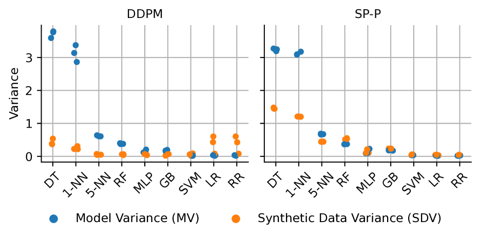
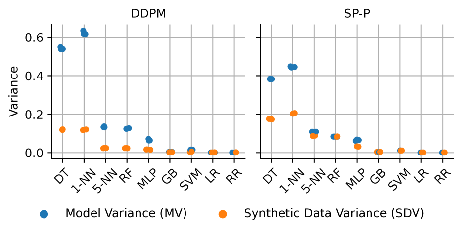
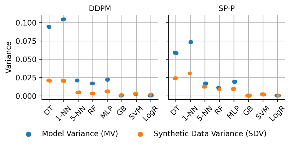
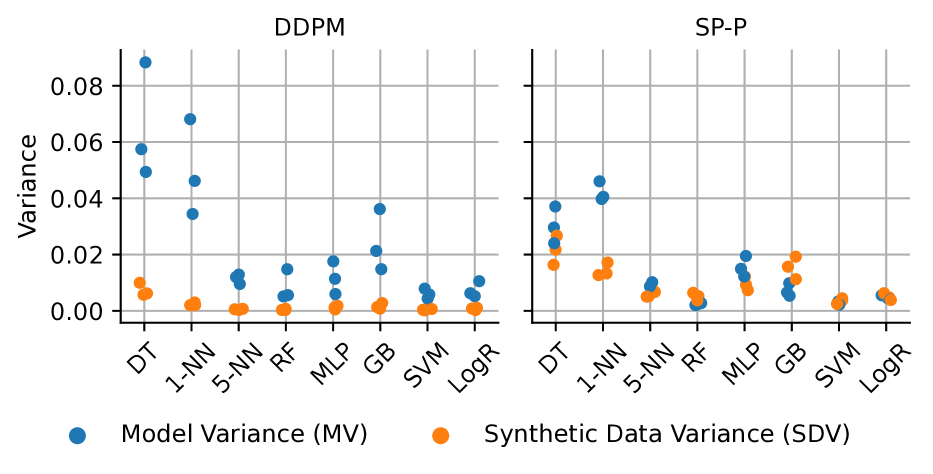
In this section, we estimate the MV and SDV terms from the decomposition in Theorem 2.2. We first generate 32 synthetic datasets that are 5 times larger than the real dataset, and split each synthetic datasets into 5 equally-sized subsets. This is equivalent to sampling 32 $\theta_{i}$ values, and for each $\theta_{i}$, generating 5 synthetic datasets i.i.d.  We then train the downstream predictor on each synthetic dataset, and store the predictions for all test points.

To estimate MV, we compute the sample variance over the 5 synthetic datasets generated from the same $\theta_{i}$, and then compute the mean over the 32 different $\theta_{i}$ values. To estimate SDV, we compute the sample mean over the 5 synthetic datasets from the same $\theta_{i}$, and compute the sample variance over the 32 different $\theta_{i}$ values.

The result is an estimate of MV and SDV for each test point. We plot the mean over the test points. The whole experiment is repeated 3 times, with different train-test splits. The datasets, train-test splits, and downstream predictors are the same as in the other experiments, described in Appendix C.

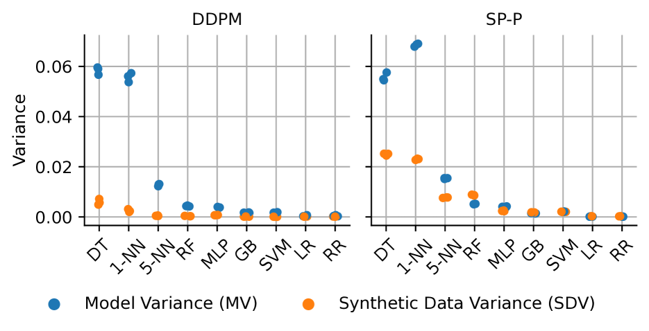
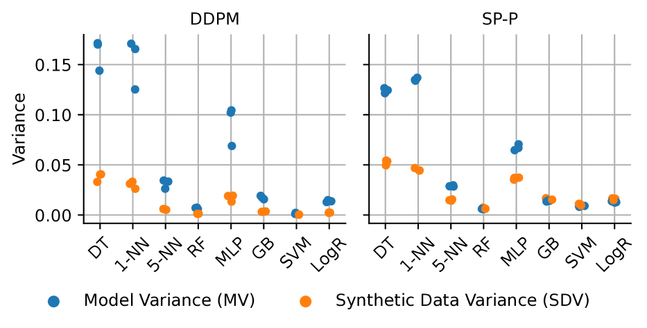
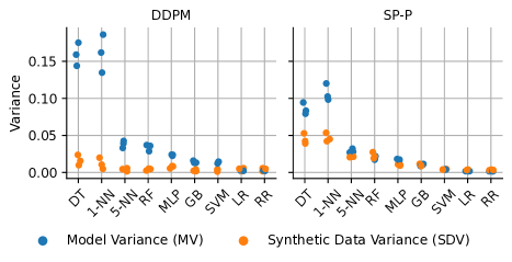
The results are in Figure 13. MV depends mostly on the downstream predictor, while SDV also depends on the synthetic data generator. We also confirm that decision trees and 1-NN have much higher variance than the other models, and linear, ridge and logistic regression have a very low variance.

(a) Abalone

(b) ACS 2018

(c) Adult

(d) Breast Cancer

(e) California Housing

(f) German Credit

(g) Insurance

Figure 13: Estimating the MV and SDV terms from the decomposition. Decision trees have high variances on all datasets, while linear, ridge and logistic regression have low variances. MV depends mostly on the predictor, while SDV depends on both the predictor and synthetic data generation algorithm. The points are the averages of estimated MV and SDV, averaged over the test data, from 3 repeats with different train-test splits. We excluded some test data points that had extremely large variance estimates ($\geq 10^{6}$) for linear regression on the ACS 2018 dataset. The predictors are decision tree (DT), nearest neighbours with 1 or 5 neighbours (1-NN and 5-NN), random forest (RF), a multilayer perceptron (MLP), gradient boosted trees (GB), a support vector machine (SVM), linear regression (LR), ridge regression (RR) and logistic regression (LogR). The synthetic data generators are DDPM and synthpop (SP-P).

References

- Antoniou et al. (2018) Antreas Antoniou, Amos Storkey, and Harrison Edwards. Data Augmentation Generative Adversarial Networks, 2018. URL http://arxiv.org/abs/1711.04340.
- Aydore et al. (2021) Sergul Aydore, William Brown, Michael Kearns, Krishnaram Kenthapadi, Luca Melis, Aaron Roth, and Ankit A Siva. Differentially Private Query Release Through Adaptive Projection. In Proceedings of the 38th International Conference on Machine Learning, volume 139 of Proceedings of Machine Learning Research, pages 457–467. PMLR, 2021. URL http://proceedings.mlr.press/v139/aydore21a.html.
- Bregman (1967) L. M. Bregman. The relaxation method of finding the common point of convex sets and its application to the solution of problems in convex programming. USSR Computational Mathematics and Mathematical Physics, 7(3):200–217, 1967. URL https://www.sciencedirect.com/science/article/pii/0041555367900407.
- Breiman (1996) Leo Breiman. Bagging predictors. Machine Learning, 24(2):123–140, 1996. URL https://doi.org/10.1007/BF00058655.
- Breiman (2001) Leo Breiman. Random Forests. Machine Learning, 45(1):5–32, 2001. URL https://doi.org/10.1023/A:1010933404324.
- Brier (1950) Glenn W Brier. Verification of forecasts expressed in terms of probability. Monthly weather review, 78(1):1–3, 1950.
- Chen et al. (2020) Dingfan Chen, Tribhuvanesh Orekondy, and Mario Fritz. GS-WGAN: A gradient-sanitized approach for learning differentially private generators. In Advances in Neural Information Processing Systems, volume 33, pages 12673–12684, 2020. URL https://proceedings.neurips.cc/paper/2020/file/9547ad6b651e2087bac67651aa92cd0d-Paper.pdf.
- Chen et al. (2023) Mingqin Chen, Yuhui Quan, Yong Xu, and Hui Ji. Self-Supervised Blind Image Deconvolution via Deep Generative Ensemble Learning. IEEE Transactions on Circuits and Systems for Video Technology, 33(2):634–647, 2023.
- Choi et al. (2019) Hyunsun Choi, Eric Jang, and Alexander A. Alemi. WAIC, but Why? Generative Ensembles for Robust Anomaly Detection, 2019. URL http://arxiv.org/abs/1810.01392.
- Das et al. (2022) Hari Prasanna Das, Ryan Tran, Japjot Singh, Xiangyu Yue, Geoffrey Tison, Alberto Sangiovanni-Vincentelli, and Costas J. Spanos. Conditional Synthetic Data Generation for Robust Machine Learning Applications with Limited Pandemic Data. In Proceedings of the AAAI Conference on Artificial Intelligence, volume 36, pages 11792–11800, 2022. URL https://ojs.aaai.org/index.php/AAAI/article/view/21435.
- Dikici et al. (2020) Engin Dikici, Luciano M. Prevedello, Matthew Bigelow, Richard D. White, and Barbaros Selnur Erdal. Constrained Generative Adversarial Network Ensembles for Sharable Synthetic Data Generation, 2020. URL http://arxiv.org/abs/2003.00086.
- Ding et al. (2021) Frances Ding, Moritz Hardt, John Miller, and Ludwig Schmidt. Retiring Adult: New Datasets for Fair Machine Learning. In Advances in Neural Information Processing Systems, volume 34, 2021. URL https://openreview.net/forum?id=bYi_2708mKK.
- Dwork and Roth (2014) Cynthia Dwork and Aaron Roth. The Algorithmic Foundations of Differential Privacy. Foundations and Trends in Theoretical Computer Science, 9(3-4):211–407, 2014. URL https://doi.org/10.1561/0400000042.
- Dwork et al. (2006) Cynthia Dwork, Frank McSherry, Kobbi Nissim, and Adam D. Smith. Calibrating Noise to Sensitivity in Private Data Analysis. In Third Theory of Cryptography Conference, volume 3876 of Lecture Notes in Computer Science, pages 265–284. Springer, 2006. URL https://doi.org/10.1007/11681878_14.
- Geman et al. (1992) Stuart Geman, Elie Bienenstock, and René Doursat. Neural Networks and the Bias/Variance Dilemma. Neural Computation, 4(1):1–58, 1992. URL https://doi.org/10.1162/neco.1992.4.1.1.
- Gneiting and Raftery (2007) Tilmann Gneiting and Adrian E Raftery. Strictly Proper Scoring Rules, Prediction, and Estimation. Journal of the American Statistical Association, 102(477):359–378, 2007. URL https://doi.org/10.1198/016214506000001437.
- Gupta et al. (2022) Neha Gupta, Jamie Smith, Ben Adlam, and Zelda E. Mariet. Ensembles of Classifiers: A Bias-Variance Perspective. Transactions on Machine Learning Research, 2022. URL https://openreview.net/forum?id=lIOQFVncY9.
- Harder et al. (2021) Frederik Harder, Kamil Adamczewski, and Mijung Park. DP-MERF: Differentially Private Mean Embeddings with RandomFeatures for Practical Privacy-preserving Data Generation. In Proceedings of The 24th International Conference on Artificial Intelligence and Statistics, volume 130 of Proceedings of Machine Learning Research, pages 1819–1827. PMLR, 2021. URL http://proceedings.mlr.press/v130/harder21a.html.
- Hardt et al. (2012) Moritz Hardt, Katrina Ligett, and Frank McSherry. A Simple and Practical Algorithm for Differentially Private Data Release. In Advances in Neural Information Processing Systems, volume 25, pages 2348–2356, 2012. URL https://proceedings.neurips.cc/paper/2012/hash/208e43f0e45c4c78cafadb83d2888cb6-Abstract.html.
- Hofmann (1994) Hans Hofmann. Statlog (German credit data). UCI Machine Learning Repository, 1994. URL https://archive.ics.uci.edu/dataset/144/statlog+german+credit+data.
- Jälkö et al. (2017) Joonas Jälkö, Onur Dikmen, and Antti Honkela. Differentially Private Variational Inference for Non-conjugate Models. In Proceedings of the Thirty-Third Conference on Uncertainty in Artificial Intelligence. AUAI Press, 2017. URL http://auai.org/uai2017/proceedings/papers/152.pdf.
- Jälkö et al. (2021) Joonas Jälkö, Eemil Lagerspetz, Jari Haukka, Sasu Tarkoma, Antti Honkela, and Samuel Kaski. Privacy-preserving data sharing via probabilistic modeling. Patterns, 2(7):100271, 2021. URL https://linkinghub.elsevier.com/retrieve/pii/S2666389921000970.
- James (2003) Gareth M. James. Variance and Bias for General Loss Functions. Machine Learning, 51(2):115–135, 2003. URL https://doi.org/10.1023/A:1022899518027.
- Kimpara et al. (2023) Dhamma Kimpara, Rafael Frongillo, and Bo Waggoner. Proper Losses for Discrete Generative Models. In Proceedings of the 40th International Conference on Machine Learning, 2023. URL https://openreview.net/forum?id=VVdb1la0cW.
- Kohavi and Becker (1996) Ronny Kohavi and Barry Becker. Adult. UCI Machine Learning Repository, 1996. URL https://archive.ics.uci.edu/dataset/2/adult.
- Kotelnikov et al. (2023) Akim Kotelnikov, Dmitry Baranchuk, Ivan Rubachev, and Artem Babenko. TabDDPM: Modelling Tabular Data with Diffusion Models. In Proceedings of the 40th International Conference on Machine Learning, 2023. URL https://openreview.net/forum?id=hTzPqLKBJY.
- Lakshminarayanan et al. (2017) Balaji Lakshminarayanan, Alexander Pritzel, and Charles Blundell. Simple and Scalable Predictive Uncertainty Estimation using Deep Ensembles. In Advances in Neural Information Processing Systems, volume 30, 2017. URL https://proceedings.neurips.cc/paper_files/paper/2017/hash/9ef2ed4b7fd2c810847ffa5fa85bce38-Abstract.html.
- Liew et al. (1985) Chong K. Liew, Uinam J. Choi, and Chung J. Liew. A data distortion by probability distribution. ACM Transactions on Database Systems, 10(3):395–411, 1985. URL https://dl.acm.org/doi/10.1145/3979.4017.
- Liu et al. (2021) Terrance Liu, Giuseppe Vietri, and Steven Z. Wu. Iterative Methods for Private Synthetic Data: Unifying Framework and New Methods. In Advances in Neural Information Processing Systems, volume 34, pages 690–702, 2021. URL https://proceedings.neurips.cc/paper/2021/hash/0678c572b0d5597d2d4a6b5bd135754c-Abstract.html.
- Luzi et al. (2020) Lorenzo Luzi, Randall Balestriero, and Richard G. Baraniuk. Ensembles of Generative Adversarial Networks for Disconnected Data, 2020. URL http://arxiv.org/abs/2006.14600.
- McKenna et al. (2019) Ryan McKenna, Daniel Sheldon, and Gerome Miklau. Graphical-model based estimation and inference for differential privacy. In Proceedings of the 36th International Conference on Machine Learning, volume 97 of Proceedings of Machine Learning Research, pages 4435–4444. PMLR, 2019. URL http://proceedings.mlr.press/v97/mckenna19a.html.
- McKenna et al. (2021) Ryan McKenna, Gerome Miklau, and Daniel Sheldon. Winning the NIST Contest: A scalable and general approach to differentially private synthetic data. Journal of Privacy and Confidentiality, 11(3), 2021. URL https://journalprivacyconfidentiality.org/index.php/jpc/article/view/778.
- Meeus et al. (2023) Matthieu Meeus, Florent Guépin, Ana-Maria Cretu, and Yves-Alexandre de Montjoye. Achilles’ Heels: Vulnerable Record Identification in Synthetic Data Publishing. In 28th European Symposium on Research in Computer Security, 2023. URL http://arxiv.org/abs/2306.10308.
- Nash et al. (1995) Warwick Nash, Tracy Sellers, Simon Talbot, Andrew Cawthorn, and Wes Ford. Abalone. UCI Machine Learning Repository, 1995. URL https://archive.ics.uci.edu/dataset/1/abalone.
- Nowok et al. (2016) Beata Nowok, Gillian M. Raab, and Chris Dibben. Synthpop: Bespoke Creation of Synthetic Data in R. Journal of Statistical Software, 74:1–26, 2016. URL https://doi.org/10.18637/jss.v074.i11.
- Pfau (2013) David Pfau. A generalized bias-variance decomposition for bregman divergences. 2013. URL http://www.davidpfau.com/assets/generalized_bvd_proof.pdf.
- Raghunathan et al. (2003) Trivellore E. Raghunathan, Jerome P. Reiter, and Donald B. Rubin. Multiple imputation for statistical disclosure limitation. Journal of Official Statistics, 19(1):1, 2003.
- Räisä et al. (2023a) Ossi Räisä, Joonas Jälkö, and Antti Honkela. On Consistent Bayesian Inference from Synthetic Data, 2023a. URL http://arxiv.org/abs/2305.16795.
- Räisä et al. (2023b) Ossi Räisä, Joonas Jälkö, Samuel Kaski, and Antti Honkela. Noise-aware statistical inference with differentially private synthetic data. In Proceedings of The 26th International Conference on Artificial Intelligence and Statistics, volume 206 of Proceedings of Machine Learning Research, pages 3620–3643. PMLR, 2023b. URL https://proceedings.mlr.press/v206/raisa23a.html.
- Rubin (1993) Donald B. Rubin. Discussion: Statistical disclosure limitation. Journal of Official Statistics, 9(2):461–468, 1993.
- Ueda and Nakano (1996) N. Ueda and R. Nakano. Generalization error of ensemble estimators. In Proceedings of International Conference on Neural Networks (ICNN’96), volume 1, pages 90–95 vol.1, 1996.
- van Breugel et al. (2021) Boris van Breugel, Trent Kyono, Jeroen Berrevoets, and Mihaela van der Schaar. DECAF: Generating Fair Synthetic Data Using Causally-Aware Generative Networks. In Advances in Neural Information Processing Systems, volume 34, pages 22221–22233, 2021. URL https://proceedings.neurips.cc/paper/2021/hash/ba9fab001f67381e56e410575874d967-Abstract.html.
- van Breugel et al. (2023a) Boris van Breugel, Zhaozhi Qian, and Mihaela van der Schaar. Synthetic data, real errors: How (not) to publish and use synthetic data. In Proceedings of the 40th International Conference on Machine Learning, volume 202 of Proceedings of Machine Learning Research, pages 34793–34808. PMLR, 2023a. URL https://proceedings.mlr.press/v202/van-breugel23a.html.
- van Breugel et al. (2023b) Boris van Breugel, Nabeel Seedat, Fergus Imrie, and Mihaela van der Schaar. Can You Rely on Your Model Evaluation? Improving Model Evaluation with Synthetic Test Data. In Thirty-Seventh Conference on Neural Information Processing Systems, 2023b. URL https://openreview.net/forum?id=tJ88RBqupo.
- van Breugel et al. (2023c) Boris van Breugel, Hao Sun, Zhaozhi Qian, and Mihaela van der Schaar. Membership Inference Attacks against Synthetic Data through Overfitting Detection. In Proceedings of The 26th International Conference on Artificial Intelligence and Statistics, pages 3493–3514. PMLR, 2023c. URL https://proceedings.mlr.press/v206/breugel23a.html.
- Wang et al. (2016) Yaxing Wang, Lichao Zhang, and Joost van de Weijer. Ensembles of Generative Adversarial Networks, 2016. URL http://arxiv.org/abs/1612.00991.
- Wilson and Izmailov (2020) Andrew G Wilson and Pavel Izmailov. Bayesian Deep Learning and a Probabilistic Perspective of Generalization. In Advances in Neural Information Processing Systems, volume 33, pages 4697–4708, 2020. URL https://proceedings.neurips.cc/paper/2020/hash/322f62469c5e3c7dc3e58f5a4d1ea399-Abstract.html.
- Wilson (2021) Andrew Gordon Wilson. Deep Ensembles as Approximate Bayesian Inference, 2021. URL https://cims.nyu.edu/~andrewgw/deepensembles/.
- Wolberg et al. (1995) William Wolberg, Olvi Mangasarian, Nick Street, and W. Street. Breast cancer Wisconsin (diagnostic). UCI Machine Learning Repository, 1995. URL https://archive.ics.uci.edu/dataset/17/breast+cancer+wisconsin+diagnostic.
- Wood et al. (2023) Danny Wood, Tingting Mu, Andrew M. Webb, Henry W. J. Reeve, Mikel Lujan, and Gavin Brown. A Unified Theory of Diversity in Ensemble Learning. Journal of Machine Learning Research, 24(359):1–49, 2023. URL http://jmlr.org/papers/v24/23-0041.html.
- Xu et al. (2019) Lei Xu, Maria Skoularidou, Alfredo Cuesta-Infante, and Kalyan Veeramachaneni. Modeling Tabular data using Conditional GAN. In Advances in Neural Information Processing Systems, volume 32, 2019. URL https://proceedings.neurips.cc/paper/2019/hash/254ed7d2de3b23ab10936522dd547b78-Abstract.html.