Continuous-time Trajectory Estimation: A Comparative Study Between Gaussian Process and Spline-based Approaches

Jacob C. Johnson1, Joshua G. Mangelson1, Timothy D. Barfoot2, Randal W. Beard1 This work has been funded by the Center for Autonomous Air Mobility and Sensing (CAAMS), a National Science Foundation Industry/University Cooperative Research Center (I/UCRC) under NSF award No. 2139551, along with significant contributions from CAAMS industry members.1J. C. Johnson, J. G. Mangelson, and R. W. Beard are with the Electrical and Computer Engineering Department at Brigham Young University, Provo, UT, 84602 USA. (e-mail: jjohns99@byu.edu).2T. D. Barfoot is with the University of Toronto Institute for Aerospace Studies, Toronto, ON, CA.
Abstract

Continuous-time trajectory estimation is an attractive alternative to discrete-time batch estimation due to the ability to incorporate high-frequency measurements from asynchronous sensors while keeping the number of optimization parameters bounded. Two types of continuous-time estimation have become prevalent in the literature: Gaussian process regression and spline-based estimation. In this paper, we present a direct comparison between these two methods. We first compare them using a simple linear system, and then compare them in a camera and IMU sensor fusion scenario on SE(3) in both simulation and hardware. Our results show that if the same measurements and motion model are used, the two methods achieve similar trajectory accuracy. In addition, if the spline order is chosen so that the degree-of-differentiability of the two trajectory representations match, then they achieve similar solve times as well.

I Introduction

State estimation is an essential area of robotics. Without an accurate estimate of a mobile robot’s dynamic state, other autonomy tasks such as online path planning and control are not possible. Traditionally, state estimation has most often been accomplished using some variant of the well-known Kalman filter (KF) [1, 2, 3, 4]. More recently, however, discrete-time batch estimation methods such as bundle adjustment [5] have gained a significant amount of popularity [6, 7, 8]. In these methods, a discrete set of past robot states is estimated simultaneously using nonlinear optimization. Batch estimation has been shown to offer better performance than traditional filtering [9], in large part because the nonlinearities in the measurement models are iteratively relinearized about the current best guess rather than linearizing only once. One drawback of discrete-time batch estimation, however, is that it is difficult to include measurements from multiple sensors that are asynchronous or that come at high frequencies. This is because each measurement used in the optimization must be tied to an optimization parameter, meaning that the number of states that must be optimized goes up linearly with the number of measurements, making the problem intractable when high-frequency sensors are used. Usually to include such sensors, the measurements are grouped and approximated in some way such as IMU preintegration [10, 11].

Within the last decade or so, continuous-time batch estimation has been introduced [12]. Rather than optimizing a discrete set of robot states, the continuous trajectory of the robot is estimated. The trajectory is represented using a discrete set of parameters and a map from these parameters to the robot state at a given time. The main advantage of continuous-time batch estimation is that the trajectory estimate can be sampled at any time, making it straightforward to incorporate measurements from asynchronous, high-frequency sensors without having to increase the number of optimization parameters. Within the continuous-time estimation literature, there are two major methods that have been proposed to represent continuous robot trajectories: splines (parametric) [12] and Gaussian processes (GPs) (nonparametric) [13].

I-1 Splines

Splines [14, 15] are piecewise polynomial functions that are characterized by a set of control points on the configuration manifold and a set of knot points in time. The differentiability of the spline is determined by the spline order, which also determines how many control points are used when evaluating the spline at a given time. When performing estimation with splines, the control point locations are optimized such that the resulting trajectory optimally fits the acquired measurements and motion priors [12]. While the original spline formulation is only suited for use on vector spaces, it is possible to generalize them for use with Lie groups [16, 17, 18], which is important for state estimation because attitude is most often represented using rotation matrices. Splines have been used for sensor fusion using inertial measurement units (IMUs) [12, 19, 20], rolling shutter cameras [21, 19], event cameras [22], radar [23], and lidar [24, 25].

I-2 GPs

Continuous trajectories can also be estimated using GP regression [13, 26]. In this method, the robot’s motion is modeled using a GP and the states at a discrete set of estimation times are optimized. The states at other measurement and query times are evaluated using GP interpolation. The interpolation scheme is derived from the model used to represent the motion of the robot. When performing GP-based estimation on Lie groups, the trajectory is modeled using a locally linear system that evolves in the Lie algebra [27]. Some models that have been used in the literature include white-noise-on-acceleration (WNOA) [27], white-noise-on-jerk (WNOJ) [28], and data-driven motion priors [29]. GP regression has been used in a variety of continuous estimation problems, including radar-based localization [30], lidar odometry using Doppler measurements [31], and even continuum robot pose estimation [32]. The idea has also been extended to continuous-time motion planning problems [33, 34].

Both splines and GPs are valid ways to represent continuous robot trajectories, and both have been used in a variety of scenarios. Their underlying representations differ in a few significant ways: the estimation parameters lie in different spaces (the configuration manifold for splines versus the state space for GPs), splines do not require the use of a motion model (although one can be used if desired), and the degree-of-differentiability is determined differently (from the chosen order for splines and from the motion model for GPs). It is unclear what advantages and disadvantages each of the methods have, or whether one should be used rather than the other in a given scenario.

To our knowledge, no formal, direct comparison between these methods exists in the literature. In this paper, we develop such a comparison, with the intent of determining the relative advantages and disadvantages of both. We introduce continuous-time trajectory estimation generally, both for linear systems on vector spaces as well as for nonlinear systems on Lie groups. In the interest of maintaining a fair and accurate comparison, we show how to generalize the motion priors introduced for GP-based estimation in [13] and [27] so that the same motion model can be used for both GPs and splines. We then compare GP and spline-based estimation directly in two different scenarios: for a simple linear WNOJ system with simulated position measurements, and for camera and IMU sensor fusion on SE(3). For the camera and IMU fusion scenario, we compare the two methods using both simulated data and hardware data in order to validate the comparison against ground truth and also with real sensor measurements.

This paper presents the following contributions:

  • a direct comparison of GP and spline-based continuous-time trajectory estimation in the case of a linear system with a linear measurement model,

  • a direct comparison of GP and spline-based estimation on SE(3) using IMU measurements and fiducial pose measurements from a camera, both with simulated and hardware data, and

  • a generalization of the linear and Lie group GP motion priors in [13, 27] for use in spline-based estimation.

The outline of this paper is as follows. Section II introduces continuous-time trajectory estimation generally and develops motion models for both linear systems and systems on Lie groups, and Sections III and IV apply this theory to GP and spline-based estimation, respectively. Section V introduces the comparison scenarios we will be using, and Sections VIVII, and VIII present the comparison results for these scenarios. Finally, we finish with some discussion and concluding remarks in Sections IX and X, respectively.

II Continuous-time Trajectory Estimation

Let 𝒳𝒳\mathcal{X} represent the state space of a dynamic system and let 𝒲=[tmin,tmax]𝒲subscript𝑡minsubscript𝑡max\mathcal{W}=[t_{\text{min}},t_{\text{max}}] represent a window of time defined by tminsubscript𝑡mint_{\text{min}}, tmaxsubscript𝑡maxt_{\text{max}}. Our objective is to find the best estimate of a continuous trajectory 𝐱(𝒲)={𝐱(t)|t𝒲}𝐱𝒲conditional-set𝐱𝑡𝑡𝒲\mathbf{x}(\mathcal{W})=\{\mathbf{x}(t)\>|\>t\in\mathcal{W}\} taken by the system given a set of measurements collected from a number of different sensors (indexed by the set 𝒮𝒮\mathcal{S}) throughout the time window. The sensors do not need to run at similar frequencies or be in phase with one another. Each measurement 𝐳issuperscriptsubscript𝐳𝑖𝑠\mathbf{z}_{i}^{s}, sS𝑠𝑆s\in S, i=1,,Ns𝑖1subscript𝑁𝑠i=1,\cdots,N_{s} for sensor s𝑠s is modeled by

𝐳is=𝐡s(𝐱(tis))+𝜼,superscriptsubscript𝐳𝑖𝑠superscript𝐡𝑠𝐱superscriptsubscript𝑡𝑖𝑠𝜼\mathbf{z}_{i}^{s}=\mathbf{h}^{s}(\mathbf{x}(t_{i}^{s}))+\boldsymbol{\eta}, (1)

where hs()superscript𝑠h^{s}(\cdot) is the measurement model, tis𝒲superscriptsubscript𝑡𝑖𝑠𝒲t_{i}^{s}\in\mathcal{W} is the measurement time, and 𝜼𝒩(𝟎,𝚺s)similar-to𝜼𝒩0subscript𝚺𝑠\boldsymbol{\eta}\sim\mathcal{N}(\mathbf{0},\boldsymbol{\Sigma}_{s}) is zero-mean Gaussian measurement noise111It is often the case that measurements 𝐳issuperscriptsubscript𝐳𝑖𝑠\mathbf{z}_{i}^{s} belong to a Lie group. Rather than using the additive noise model (1), we perturb the measurement with noise in either the left or the right tangent space, e.g., 𝐳is=Exp(𝜼)hs()superscriptsubscript𝐳𝑖𝑠Exp𝜼superscript𝑠\mathbf{z}_{i}^{s}=\text{Exp}(\boldsymbol{\eta})h^{s}(\cdot) [35]. with covariance 𝚺ssubscript𝚺𝑠\boldsymbol{\Sigma}_{s}.

The goal of continuous-time estimation is to find the continuous state trajectory 𝐱(𝒲)𝐱𝒲\mathbf{x}(\mathcal{W}) that solves the maximum-a-posteriori problem

max𝐱(𝒲)p(𝐱(𝒲))|𝐳)p(𝐳|𝐱(𝒲))p(𝐱(𝒲)),\max_{\mathbf{x}(\mathcal{W})}p(\mathbf{x}(\mathcal{W}))|\mathbf{z})\propto p(\mathbf{z}|\mathbf{x}(\mathcal{W}))p(\mathbf{x}(\mathcal{W})), (2)

where 𝐳={𝐳is}sS,i=1,,Ns𝐳subscriptsuperscriptsubscript𝐳𝑖𝑠formulae-sequence𝑠𝑆𝑖1subscript𝑁𝑠\mathbf{z}=\{\mathbf{z}_{i}^{s}\}_{s\in S,i=1,\cdots,N_{s}}, and the prior term p(𝐱(𝒲))𝑝𝐱𝒲p(\mathbf{x}(\mathcal{W})) represents a continuous Markov process. This is an infinite-dimensional estimation problem. Rather than solve it in this form, we will represent 𝐱(𝒲)𝐱𝒲\mathbf{x}(\mathcal{W}) using a discrete set of estimation parameters {𝐱¯n}n=1,,Nsubscriptsubscript¯𝐱𝑛𝑛1𝑁\{\bar{\mathbf{x}}_{n}\in\mathcal{E}\}_{n=1,\cdots,N} (where \mathcal{E} is the estimation parameter space) and a function ι:𝒲×N𝒳:𝜄𝒲superscript𝑁𝒳\iota:\mathcal{W}\times\mathcal{E}^{N}\rightarrow\mathcal{X} such that

𝐱(t)=ι(t,{𝐱¯n}).𝐱𝑡𝜄𝑡subscript¯𝐱𝑛\mathbf{x}(t)=\iota(t,\{\bar{\mathbf{x}}_{n}\}). (3)

We will refer to ι()𝜄\iota(\cdot) as the state interpolation function. In addition, the prior term p(𝐱(𝒲))𝑝𝐱𝒲p(\mathbf{x}(\mathcal{W})) must be approximated. We will do this using a discrete set of motion priors at the motion sample times {tj𝒲}j=1,,Nmsubscriptsuperscriptsubscript𝑡𝑗𝒲𝑗1subscript𝑁𝑚\{t_{j}^{\prime}\in\mathcal{W}\}_{j=1,\cdots,N_{m}}. These motion priors will be of the form

𝐦(𝐱(tj),𝐱(tj+1))𝐦𝐱superscriptsubscript𝑡𝑗𝐱superscriptsubscript𝑡𝑗1\mathbf{m}\left(\mathbf{x}(t_{j}^{\prime}),\mathbf{x}(t_{j+1}^{\prime})\right) (4)

with covariance 𝐐tj+1subscript𝐐superscriptsubscript𝑡𝑗1{\mathbf{Q}_{t_{j+1}^{\prime}}}. We explain how these motion priors can be derived for certain model types in Section II-A.

If the measurements are independent of one another and are only dependent on the state at the time the measurement was acquired, then (2) becomes222In the case that a measurement 𝐳issuperscriptsubscript𝐳𝑖𝑠\mathbf{z}_{i}^{s} belongs to a Lie group, we replace the inside of the norm in (5) with Log(𝐳ishs()1)Logsuperscriptsubscript𝐳𝑖𝑠superscript𝑠superscript1\text{Log}\left(\mathbf{z}_{i}^{s}h^{s}(\cdot)^{-1}\right).

{𝐱¯}n=argmin{𝐱¯}nsSi=1Ns𝐳is𝐡s(ι(tis,{𝐱¯n}))𝚺s12+j=1Nm1𝐦(ι(tj,{𝐱¯n}),ι(tj+1,{𝐱¯n}))𝐐tj+112,subscriptsuperscript¯𝐱𝑛subscriptargminsubscript¯𝐱𝑛subscript𝑠𝑆superscriptsubscript𝑖1subscript𝑁𝑠subscriptsuperscriptdelimited-∥∥superscriptsubscript𝐳𝑖𝑠superscript𝐡𝑠𝜄superscriptsubscript𝑡𝑖𝑠subscript¯𝐱𝑛2superscriptsubscript𝚺𝑠1superscriptsubscript𝑗1subscript𝑁𝑚1subscriptsuperscriptdelimited-∥∥𝐦𝜄superscriptsubscript𝑡𝑗subscript¯𝐱𝑛𝜄superscriptsubscript𝑡𝑗1subscript¯𝐱𝑛2superscriptsubscript𝐐superscriptsubscript𝑡𝑗11\begin{split}\{\bar{\mathbf{x}}^{\ast}\}_{n}&=\operatorname*{arg\,min}_{\{\bar{\mathbf{x}}\}_{n}}\sum_{s\in S}\sum_{i=1}^{N_{s}}\lVert\mathbf{z}_{i}^{s}-\mathbf{h}^{s}\left(\iota(t_{i}^{s},\{\bar{\mathbf{x}}_{n}\})\right)\rVert^{2}_{\boldsymbol{\Sigma}_{s}^{-1}}\\ &\quad+\sum_{j=1}^{N_{m}-1}\lVert\mathbf{m}\left(\iota(t_{j}^{\prime},\{\bar{\mathbf{x}}_{n}\}),\iota(t_{j+1}^{\prime},\{\bar{\mathbf{x}}_{n}\})\right)\rVert^{2}_{\mathbf{Q}_{t_{j+1}^{\prime}}^{-1}},\end{split} (5)

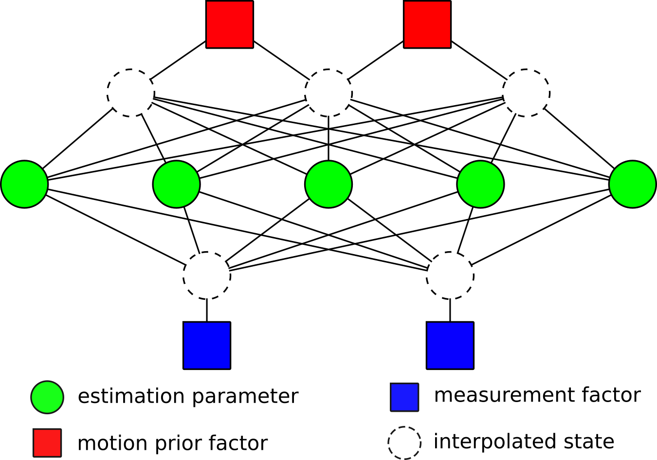
where 𝐖subscriptdelimited-∥∥𝐖\lVert\cdot\rVert_{\mathbf{W}} indicates the 2-norm weighted by the matrix 𝐖𝐖\mathbf{W}. An example factor graph for this problem is shown in Figure 1.
Refer to caption
Figure 1: Example factor graph for the continuous-time estimation problem (5). The interpolated states are not directly optimized, rather they are computed from the estimation parameters using the state interpolation function (3).
Note 1

The graph in Figure 1 is dense with respect to the estimation parameters because the general interpolation function (3) is dependent on every parameter. This need not be the case, however. The state interpolation methods used in Sections III and IV are chosen such that the interpolation is only dependent on a few of the parameters in order to make the problem more sparse.

II-A Motion Priors

To approximate the prior term p(𝐱(𝒲))𝑝𝐱𝒲p(\mathbf{x}(\mathcal{W})) in (2), we will assume that the state 𝐱𝐱\mathbf{x} evolves according to a certain stochastic model. We will first consider linear models and then show how this formulation can be extended to Lie groups. These motion priors were originally presented in [13, 27, 28] for GP-based estimation. Here we generalize them so they can be used in spline-based estimation as well.

II-A1 Linear systems

We restrict our attention to time-invariant systems for simplicity. Assume that the state evolves according to

𝐱˙(t)=𝐀𝐱(t)+𝐁𝐮(𝐭)+𝐋𝐰(t),˙𝐱𝑡𝐀𝐱𝑡𝐁𝐮𝐭𝐋𝐰𝑡\dot{\mathbf{x}}(t)=\mathbf{A}\mathbf{x}(t)+\mathbf{B}\mathbf{u(t)}+\mathbf{L}\mathbf{w}(t), (6)

where 𝐀𝐀\mathbf{A}, 𝐁𝐁\mathbf{B}, and 𝐋𝐋\mathbf{L} are the system matrices, 𝐮(t)𝐮𝑡\mathbf{u}(t) is a known system input, and 𝐰(t)𝒢𝒫(𝟎,𝐐δ(tτ))similar-to𝐰𝑡𝒢𝒫0𝐐𝛿𝑡𝜏\mathbf{w}(t)\sim\mathcal{GP}(\mathbf{0},\mathbf{Q}\delta(t-\tau)) is a stationary GP with power spectral density 𝐐𝐐\mathbf{Q}. The state transition matrix of the system is

𝚽(t,τ)=exp(𝐀(tτ)),𝚽𝑡𝜏exp𝐀𝑡𝜏\boldsymbol{\Phi}(t,\tau)=\text{exp}(\mathbf{A}(t-\tau)), (7)

where exp()exp\text{exp}(\cdot) is the matrix exponential. If we have a guess for an initial state 𝐱ˇ(t0)ˇ𝐱subscript𝑡0\check{\mathbf{x}}(t_{0}), then the prior mean function is

𝐱ˇ(t)=𝚽(t,t0)𝐱ˇ0+t0t𝚽(t,s)𝐁𝐮(s)𝑑s.ˇ𝐱𝑡𝚽𝑡subscript𝑡0subscriptˇ𝐱0superscriptsubscriptsubscript𝑡0𝑡𝚽𝑡𝑠𝐁𝐮𝑠differential-d𝑠\check{\mathbf{x}}(t)=\boldsymbol{\Phi}(t,t_{0})\check{\mathbf{x}}_{0}+\int_{t_{0}}^{t}\boldsymbol{\Phi}(t,s)\mathbf{B}\mathbf{u}(s)ds. (8)

Because 𝐱(t)𝐱𝑡\mathbf{x}(t) is a GP, the prior term p(𝐱(t))𝑝𝐱𝑡p(\mathbf{x}(t)) sampled at any time τ𝜏\tau is

p(𝐱(τ))exp(12(𝐱(τ)𝐱ˇ(τ))𝐏ˇ(τ,τ)1(𝐱(τ)𝐱ˇ(τ))),proportional-to𝑝𝐱𝜏exp12superscript𝐱𝜏ˇ𝐱𝜏topˇ𝐏superscript𝜏𝜏1𝐱𝜏ˇ𝐱𝜏\begin{split}&p(\mathbf{x}(\tau))\propto\\ &\quad\text{exp}\left(\frac{1}{2}(\mathbf{x}(\tau)-\check{\mathbf{x}}(\tau))^{\top}\check{\mathbf{P}}(\tau,\tau)^{-1}(\mathbf{x}(\tau)-\check{\mathbf{x}}(\tau))\right),\end{split} (9)

where 𝐏ˇ(τ,τ)ˇ𝐏𝜏𝜏\check{\mathbf{P}}(\tau,\tau) is the prior covariance at τ𝜏\tau. It can be shown [13] that, for τ=tj+1𝜏superscriptsubscript𝑡𝑗1\tau=t_{j+1}^{\prime}, (9) is equivalent to

exp(12𝐦(𝐱(tj),𝐱(tj+1))𝐐tj+11𝐦(𝐱(tj),𝐱(tj+1))),exp12𝐦superscript𝐱superscriptsubscript𝑡𝑗𝐱superscriptsubscript𝑡𝑗1topsuperscriptsubscript𝐐superscriptsubscript𝑡𝑗11𝐦𝐱superscriptsubscript𝑡𝑗𝐱superscriptsubscript𝑡𝑗1\text{exp}\left(\frac{1}{2}\mathbf{m}\left(\mathbf{x}(t_{j}^{\prime}),\mathbf{x}(t_{j+1}^{\prime})\right)^{\top}\mathbf{Q}_{t_{j+1}^{\prime}}^{-1}\mathbf{m}\left(\mathbf{x}(t_{j}^{\prime}),\mathbf{x}(t_{j+1}^{\prime})\right)\right), (10)

where333If there is no known input 𝐮(t)𝐮𝑡\mathbf{u}(t) to the system, then the prior terms in (11) cancel out.

𝐦(𝐱(tj),𝐱(tj+1))=𝐱(tj+1)𝐱ˇ(tj+1)𝚽(tj+1,tj)(𝐱(tj)𝐱ˇ(tj))𝐦𝐱superscriptsubscript𝑡𝑗𝐱superscriptsubscript𝑡𝑗1𝐱superscriptsubscript𝑡𝑗1ˇ𝐱superscriptsubscript𝑡𝑗1𝚽superscriptsubscript𝑡𝑗1superscriptsubscript𝑡𝑗𝐱superscriptsubscript𝑡𝑗ˇ𝐱superscriptsubscript𝑡𝑗\begin{split}&\mathbf{m}\left(\mathbf{x}(t_{j}^{\prime}),\mathbf{x}(t_{j+1}^{\prime})\right)=\\ &\qquad\mathbf{x}(t_{j+1}^{\prime})-\check{\mathbf{x}}(t_{j+1}^{\prime})-\boldsymbol{\Phi}(t_{j+1}^{\prime},t_{j}^{\prime})(\mathbf{x}(t_{j}^{\prime})-\check{\mathbf{x}}(t_{j}^{\prime}))\end{split} (11)

and, for ν[tj,tj+1]𝜈superscriptsubscript𝑡𝑗superscriptsubscript𝑡𝑗1\nu\in[t_{j}^{\prime},t_{j+1}^{\prime}],

𝐐ν=0νtj𝚽(νtj,s)𝐋𝐐𝐋𝚽(νtj,s)𝑑s.subscript𝐐𝜈superscriptsubscript0𝜈superscriptsubscript𝑡𝑗𝚽𝜈superscriptsubscript𝑡𝑗𝑠superscript𝐋𝐐𝐋top𝚽superscript𝜈superscriptsubscript𝑡𝑗𝑠topdifferential-d𝑠\mathbf{Q}_{\nu}=\int_{0}^{\nu-t_{j}^{\prime}}\boldsymbol{\Phi}(\nu-t_{j}^{\prime},s)\mathbf{L}\mathbf{Q}\mathbf{L}^{\top}\boldsymbol{\Phi}(\nu-t_{j}^{\prime},s)^{\top}ds. (12)

II-A2 Lie groups

Let G𝐺G be a matrix Lie group of dimension d𝑑d with Lie algebra 𝔤𝔤\mathfrak{g}. We will break the trajectory g(𝒲)G×𝒲𝑔𝒲𝐺𝒲g(\mathcal{W})\in G\times\mathcal{W} into segments between motion sample times and assume that the system obeys a linear stochastic model in the Lie algebra in each of these segments [27]. Specifically, we restrict our attention to a WNOJ model for simplicity444This can easily be simplified to a WNOA model by ignoring the second derivative terms and applying noise to the second derivative rather than the third. [28]. Let the state be 𝐱(t)={g(t),g˙(t),g¨(t)}G×d×d𝐱𝑡𝑔𝑡˙𝑔𝑡¨𝑔𝑡𝐺superscript𝑑superscript𝑑\mathbf{x}(t)=\{g(t),\dot{g}(t),\ddot{g}(t)\}\in G\times\mathbb{R}^{d}\times\mathbb{R}^{d}, where g˙(t)˙𝑔𝑡\dot{g}(t) is represented as an infinitesimal perturbation in the left tangent space of g(t)𝑔𝑡g(t) and g¨(t)=ddtg˙(t)¨𝑔𝑡𝑑𝑑𝑡˙𝑔𝑡\ddot{g}(t)=\frac{d}{dt}\dot{g}(t). Without loss of generality assume that t[tj,tj+1]𝑡superscriptsubscript𝑡𝑗superscriptsubscript𝑡𝑗1t\in[t_{j}^{\prime},t_{j+1}^{\prime}], and let

𝝃j(t)=Log(g(t)g(tj)1),subscript𝝃𝑗𝑡Log𝑔𝑡𝑔superscriptsuperscriptsubscript𝑡𝑗1\boldsymbol{\xi}_{j}(t)=\text{Log}\left(g(t)g(t_{j}^{\prime})^{-1}\right), (13)

where Log=log\text{Log}=\vee\circ\text{log}, :𝔤d\vee:\mathfrak{g}\rightarrow\mathbb{R}^{d} is the vee map from the Lie algebra, and log:G𝔤:log𝐺𝔤\text{log}:G\rightarrow\mathfrak{g} is the logarithmic map of G𝐺G. If 𝝃j(t)subscript𝝃𝑗𝑡\boldsymbol{\xi}_{j}(t) evolves according to a WNOJ model, then

𝜸˙j(t)=[𝟎𝐈𝟎𝟎𝟎𝐈𝟎𝟎𝟎]𝜸j(t)+[𝟎𝟎𝐈]𝐰(t),subscript˙𝜸𝑗𝑡matrix0𝐈000𝐈000subscript𝜸𝑗𝑡matrix00𝐈𝐰𝑡\dot{\boldsymbol{\gamma}}_{j}(t)=\begin{bmatrix}\mathbf{0}&\mathbf{I}&\mathbf{0}\\ \mathbf{0}&\mathbf{0}&\mathbf{I}\\ \mathbf{0}&\mathbf{0}&\mathbf{0}\end{bmatrix}\boldsymbol{\gamma}_{j}(t)+\begin{bmatrix}\mathbf{0}\\ \mathbf{0}\\ \mathbf{I}\end{bmatrix}\mathbf{w}(t), (14)

where 𝜸j(t)=[𝝃j(t)𝝃˙j(t)𝝃¨j(t)]subscript𝜸𝑗𝑡superscriptmatrixsubscript𝝃𝑗superscript𝑡topsubscript˙𝝃𝑗superscript𝑡topsubscript¨𝝃𝑗superscript𝑡toptop\boldsymbol{\gamma}_{j}(t)=\begin{bmatrix}\boldsymbol{\xi}_{j}(t)^{\top}&\dot{\boldsymbol{\xi}}_{j}(t)^{\top}&\ddot{\boldsymbol{\xi}}_{j}(t)^{\top}\end{bmatrix}^{\top} and 𝐰(t)𝒢𝒫(𝟎,𝐐δ(tτ))similar-to𝐰𝑡𝒢𝒫0𝐐𝛿𝑡𝜏\mathbf{w}(t)\sim\mathcal{GP}(\mathbf{0},\mathbf{Q}\delta(t-\tau)). We can express this system in terms of global variables using (13) and its time derivatives

𝝃˙j(t)=Jl1(𝝃j(t))g˙(t)𝝃¨j(t)=Jl1(𝝃j(t))g¨(t)+ddt(Jl1(𝝃j(t)))g˙(t)Jl1(𝝃j(t))g¨(t)12𝝃˙j(t)g˙(t),subscript˙𝝃𝑗𝑡superscriptsubscript𝐽𝑙1subscript𝝃𝑗𝑡˙𝑔𝑡subscript¨𝝃𝑗𝑡absentsuperscriptsubscript𝐽𝑙1subscript𝝃𝑗𝑡¨𝑔𝑡𝑑𝑑𝑡superscriptsubscript𝐽𝑙1subscript𝝃𝑗𝑡˙𝑔𝑡missing-subexpressionabsentsuperscriptsubscript𝐽𝑙1subscript𝝃𝑗𝑡¨𝑔𝑡12subscript˙𝝃𝑗superscript𝑡˙𝑔𝑡\begin{gathered}\dot{\boldsymbol{\xi}}_{j}(t)=J_{l}^{-1}(\boldsymbol{\xi}_{j}(t))\dot{g}(t)\\ \begin{aligned} \ddot{\boldsymbol{\xi}}_{j}(t)&=J_{l}^{-1}(\boldsymbol{\xi}_{j}(t))\ddot{g}(t)+\frac{d}{dt}\left(J_{l}^{-1}(\boldsymbol{\xi}_{j}(t))\right)\dot{g}(t)\\ &\approx J_{l}^{-1}(\boldsymbol{\xi}_{j}(t))\ddot{g}(t)-\frac{1}{2}\dot{\boldsymbol{\xi}}_{j}(t)^{\curlywedge}\dot{g}(t),\end{aligned}\end{gathered} (15)

(see Appendix -B or [28] for the derivation), where Jl()subscript𝐽𝑙J_{l}(\cdot) is the left Jacobian of G𝐺G, Jl1()superscriptsubscript𝐽𝑙1J_{l}^{-1}(\cdot) is its inverse, and :𝔤ad(𝔤)\curlywedge:\mathfrak{g}\to\text{ad}(\mathfrak{g}) maps elements of 𝔤𝔤\mathfrak{g} to their adjoint representation.

In the Lie algebra, the motion priors take the same form as (11), with

𝚽(t,tj)=[𝐈(ttj)𝐈12(ttj)2𝐈𝟎𝐈(ttj)𝐈𝟎𝟎𝐈],𝚽𝑡superscriptsubscript𝑡𝑗matrix𝐈𝑡superscriptsubscript𝑡𝑗𝐈12superscript𝑡superscriptsubscript𝑡𝑗2𝐈0𝐈𝑡superscriptsubscript𝑡𝑗𝐈00𝐈\displaystyle\boldsymbol{\Phi}(t,t_{j}^{\prime})=\begin{bmatrix}\mathbf{I}&(t-t_{j}^{\prime})\mathbf{I}&\frac{1}{2}{(t-t_{j}^{\prime})}^{2}\mathbf{I}\\ \mathbf{0}&\mathbf{I}&(t-t_{j}^{\prime})\mathbf{I}\\ \mathbf{0}&\mathbf{0}&\mathbf{I}\end{bmatrix}, (16)
𝐐ν=[120(νtj)5𝐐18(νtj)4𝐐16(νtj)3𝐐18(νtj)4𝐐13(νtj)3𝐐12(νtj)2𝐐16(νtj)3𝐐12(νtj)2𝐐(νtj)𝐐],subscript𝐐𝜈matrix120superscript𝜈superscriptsubscript𝑡𝑗5𝐐18superscript𝜈superscriptsubscript𝑡𝑗4𝐐16superscript𝜈superscriptsubscript𝑡𝑗3𝐐18superscript𝜈superscriptsubscript𝑡𝑗4𝐐13superscript𝜈superscriptsubscript𝑡𝑗3𝐐12superscript𝜈superscriptsubscript𝑡𝑗2𝐐16superscript𝜈superscriptsubscript𝑡𝑗3𝐐12superscript𝜈superscriptsubscript𝑡𝑗2𝐐𝜈superscriptsubscript𝑡𝑗𝐐\displaystyle\mathbf{Q}_{\nu}=\begin{bmatrix}\frac{1}{20}{(\nu-t_{j}^{\prime})}^{5}\mathbf{Q}&\frac{1}{8}{(\nu-t_{j}^{\prime})}^{4}\mathbf{Q}&\frac{1}{6}{(\nu-t_{j}^{\prime})}^{3}\mathbf{Q}\\ \frac{1}{8}{(\nu-t_{j}^{\prime})}^{4}\mathbf{Q}&\frac{1}{3}{(\nu-t_{j}^{\prime})}^{3}\mathbf{Q}&\frac{1}{2}{(\nu-t_{j}^{\prime})}^{2}\mathbf{Q}\\ \frac{1}{6}{(\nu-t_{j}^{\prime})}^{3}\mathbf{Q}&\frac{1}{2}{(\nu-t_{j}^{\prime})}^{2}\mathbf{Q}&(\nu-t_{j}^{\prime})\mathbf{Q}\end{bmatrix}, (17)

for ν[tj,tj+1]𝜈superscriptsubscript𝑡𝑗superscriptsubscript𝑡𝑗1\nu\in[t_{j}^{\prime},t_{j+1}^{\prime}]. Converting to global variables, we get

𝐦(𝐱(tj),𝐱(tj+1))=[𝝃j(tj+1)Δtg˙(tj)12Δt2g¨(tj)𝝃˙j(tj+1)g˙(tj)Δtg¨(tj)Jl1(𝝃j(tj+1))g¨(tj+1)12𝝃˙j(tj+1)g˙(tj+1)g¨(tj)]𝐦𝐱superscriptsubscript𝑡𝑗𝐱superscriptsubscript𝑡𝑗1matrixsubscript𝝃𝑗superscriptsubscript𝑡𝑗1Δ𝑡˙𝑔superscriptsubscript𝑡𝑗12Δsuperscript𝑡2¨𝑔superscriptsubscript𝑡𝑗subscript˙𝝃𝑗superscriptsubscript𝑡𝑗1˙𝑔superscriptsubscript𝑡𝑗Δ𝑡¨𝑔superscriptsubscript𝑡𝑗superscriptsubscript𝐽𝑙1subscript𝝃𝑗superscriptsubscript𝑡𝑗1¨𝑔superscriptsubscript𝑡𝑗112subscript˙𝝃𝑗superscriptsuperscriptsubscript𝑡𝑗1˙𝑔superscriptsubscript𝑡𝑗1¨𝑔superscriptsubscript𝑡𝑗\begin{split}&\mathbf{m}\left(\mathbf{x}(t_{j}^{\prime}),\mathbf{x}(t_{j+1}^{\prime})\right)=\\ &\quad\begin{bmatrix}\boldsymbol{\xi}_{j}(t_{j+1}^{\prime})-\Delta t\dot{g}(t_{j}^{\prime})-\frac{1}{2}\Delta t^{2}\ddot{g}(t_{j}^{\prime})\\ \dot{\boldsymbol{\xi}}_{j}(t_{j+1}^{\prime})-\dot{g}(t_{j}^{\prime})-\Delta t\ddot{g}(t_{j}^{\prime})\\ J_{l}^{-1}(\boldsymbol{\xi}_{j}(t_{j+1}^{\prime}))\ddot{g}(t_{j+1}^{\prime})-\frac{1}{2}\dot{\boldsymbol{\xi}}_{j}(t_{j+1}^{\prime})^{\curlywedge}\dot{g}(t_{j+1}^{\prime})-\ddot{g}(t_{j}^{\prime})\end{bmatrix}\end{split} (18)

where Δt=tj+1tjΔ𝑡superscriptsubscript𝑡𝑗1superscriptsubscript𝑡𝑗\Delta t=t_{j+1}^{\prime}-t_{j}^{\prime}, 𝝃j(tj+1)=Log(g(tj+1)g(tj)1)subscript𝝃𝑗superscriptsubscript𝑡𝑗1Log𝑔superscriptsubscript𝑡𝑗1𝑔superscriptsuperscriptsubscript𝑡𝑗1\boldsymbol{\xi}_{j}(t_{j+1}^{\prime})=\text{Log}\left(g(t_{j+1}^{\prime})g(t_{j}^{\prime})^{-1}\right), and 𝝃˙j(tj+1)=Jl1(𝝃j(tj+1))g˙(tj+1)subscript˙𝝃𝑗superscriptsubscript𝑡𝑗1superscriptsubscript𝐽𝑙1subscript𝝃𝑗superscriptsubscript𝑡𝑗1˙𝑔superscriptsubscript𝑡𝑗1\dot{\boldsymbol{\xi}}_{j}(t_{j+1}^{\prime})=J_{l}^{-1}(\boldsymbol{\xi}_{j}(t_{j+1}^{\prime}))\dot{g}(t_{j+1}^{\prime}). The Jacobians for these motion priors are derived in Appendix -F.

III Gaussian Process Regression

We will first look at Gaussian process (GP) regression as a method for performing continuous-time estimation. We introduce the state interpolation function for GPs on linear systems in Section III-A, and then for Lie groups in Section III-B. Finally, we explain how to use GPs in estimation problems in Section III-C. For a more in-depth treatment of GP regression for continuous-time estimation, see [36].

The GP interpolation approach is similar to spline interpolation in that it can be derived by representing the state trajectory using an arbitrary set of basis functions (i.e., the weight-space formulation in [37]); however, the interpolation equation can be manipulated into a form that is non-parametric. We will not show this derivation here for the sake of brevity, but invite the reader to see [37, 38] for more details.

III-A Linear Systems

Choose a set of estimation times {tn𝒲}n=0,,N1subscriptsubscript𝑡𝑛𝒲𝑛0𝑁1\{t_{n}\in\mathcal{W}\}_{n=0,\cdots,N-1}. The state estimates at these times {𝐱¯n=𝐱(tn)}n=0,,N1subscriptsubscript¯𝐱𝑛𝐱subscript𝑡𝑛𝑛0𝑁1\{\bar{\mathbf{x}}_{n}=\mathbf{x}(t_{n})\}_{n=0,\cdots,N-1} will be the estimation parameters that govern the trajectory estimate. Assume that the state 𝐱(t)𝐱𝑡\mathbf{x}(t) evolves according to (6). We would like to sample the trajectory at some arbitrary time τ[tn,tn+1]𝜏subscript𝑡𝑛subscript𝑡𝑛1\mathbf{\tau}\in[t_{n},t_{n+1}] using the estimation parameters. It can be shown [13] that the posterior mean function of the GP evaluated at τ𝜏\tau given the estimation parameters is

𝐱(τ)=𝐱ˇ(τ)+𝚲(τ)(𝐱¯n𝐱ˇn)+𝛀(τ)(𝐱¯n+1𝐱ˇn+1),𝐱𝜏ˇ𝐱𝜏𝚲𝜏subscript¯𝐱𝑛subscriptˇ𝐱𝑛𝛀𝜏subscript¯𝐱𝑛1subscriptˇ𝐱𝑛1\mathbf{x}(\tau)=\check{\mathbf{x}}(\tau)+\boldsymbol{\Lambda}(\tau)(\bar{\mathbf{x}}_{n}-\check{\mathbf{x}}_{n})+\boldsymbol{\Omega}(\tau)(\bar{\mathbf{x}}_{n+1}-\check{\mathbf{x}}_{n+1}), (19)

where

𝛀(τ)=𝐐τ𝚽(tn+1,τ)𝐐tn+11,𝚲(τ)=𝚽(τ,tn)𝛀(τ)𝚽(tn+1,tn),formulae-sequence𝛀𝜏subscript𝐐𝜏𝚽superscriptsubscript𝑡𝑛1𝜏topsuperscriptsubscript𝐐subscript𝑡𝑛11𝚲𝜏𝚽𝜏subscript𝑡𝑛𝛀𝜏𝚽subscript𝑡𝑛1subscript𝑡𝑛\begin{gathered}\boldsymbol{\Omega}(\tau)=\mathbf{Q}_{\tau}\boldsymbol{\Phi}(t_{n+1},\tau)^{\top}\mathbf{Q}_{t_{n+1}}^{-1},\\ \boldsymbol{\Lambda}(\tau)=\boldsymbol{\Phi}(\tau,t_{n})-\boldsymbol{\Omega}(\tau)\boldsymbol{\Phi}(t_{n+1},t_{n}),\end{gathered} (20)

𝐐τsubscript𝐐𝜏\mathbf{Q}_{\tau} and 𝐐tn+1subscript𝐐subscript𝑡𝑛1\mathbf{Q}_{t_{n+1}} are defined as in (12), and the prior mean 𝐱ˇn=𝐱ˇ(tn)subscriptˇ𝐱𝑛ˇ𝐱subscript𝑡𝑛\check{\mathbf{x}}_{n}=\check{\mathbf{x}}(t_{n}) was defined in (8). This can be simplified if no information is known about the input 𝐮(t)𝐮𝑡\mathbf{u}(t). Then the integral term in the prior mean function (8) vanishes, the prior terms in the interpolation function (19) cancel out, and (19) becomes

𝐱(τ)=𝚲(τ)𝐱¯n+𝛀(τ)𝐱¯n+1.𝐱𝜏𝚲𝜏subscript¯𝐱𝑛𝛀𝜏subscript¯𝐱𝑛1\mathbf{x}(\tau)=\boldsymbol{\Lambda}(\tau)\bar{\mathbf{x}}_{n}+\boldsymbol{\Omega}(\tau)\bar{\mathbf{x}}_{n+1}. (21)
Note 2

Interestingly, it is also possible to arrive at (19) using an optimal control perspective. See Appendix -A.

III-B Lie Groups

For an arbitrary Lie group G𝐺G, we will again use the WNOJ motion model introduced in Section II-A2. Given the set of estimation times {tn𝒲}n=0,,N1subscriptsubscript𝑡𝑛𝒲𝑛0𝑁1\{t_{n}\in\mathcal{W}\}_{n=0,\cdots,N-1}, the estimation parameters will be the states at these times {𝐱¯n={g¯n,g¯˙n,g¯¨n}G×d×d}n=0,,N1subscriptsubscript¯𝐱𝑛subscript¯𝑔𝑛subscript˙¯𝑔𝑛subscript¨¯𝑔𝑛𝐺superscript𝑑superscript𝑑𝑛0𝑁1\left\{\bar{\mathbf{x}}_{n}=\{\bar{g}_{n},\dot{\bar{g}}_{n},\ddot{\bar{g}}_{n}\}\in G\times\mathbb{R}^{d}\times\mathbb{R}^{d}\right\}_{n=0,\cdots,N-1}, where g¯n=g(tn)subscript¯𝑔𝑛𝑔subscript𝑡𝑛\bar{g}_{n}=g(t_{n}), g¯˙n=g˙(tn)subscript˙¯𝑔𝑛˙𝑔subscript𝑡𝑛\dot{\bar{g}}_{n}=\dot{g}(t_{n}), and g¯¨n=g¨(tn)subscript¨¯𝑔𝑛¨𝑔subscript𝑡𝑛\ddot{\bar{g}}_{n}=\ddot{g}(t_{n}). Let t[tn,tn+1]𝑡subscript𝑡𝑛subscript𝑡𝑛1t\in[t_{n},t_{n+1}], and define

𝝃n(t)=Log(g(t)g¯n1),subscript𝝃𝑛𝑡Log𝑔𝑡superscriptsubscript¯𝑔𝑛1\boldsymbol{\xi}_{n}(t)=\text{Log}\left(g(t)\bar{g}_{n}^{-1}\right), (22)

as was done in (13). Then 𝜸n(t)=[𝝃n(t)𝝃˙n(t)𝝃¨n(t)]subscript𝜸𝑛𝑡superscriptmatrixsubscript𝝃𝑛superscript𝑡topsubscript˙𝝃𝑛superscript𝑡topsubscript¨𝝃𝑛superscript𝑡toptop\boldsymbol{\gamma}_{n}(t)=\begin{bmatrix}\boldsymbol{\xi}_{n}(t)^{\top}&\dot{\boldsymbol{\xi}}_{n}(t)^{\top}&\ddot{\boldsymbol{\xi}}_{n}(t)^{\top}\end{bmatrix}^{\top} evolves according to (14), and its state interpolation function can be defined using (21),

𝜸n(τ)=𝚲(τ)𝜸n(tn)+𝛀(τ)𝜸n(tn+1),subscript𝜸𝑛𝜏𝚲𝜏subscript𝜸𝑛subscript𝑡𝑛𝛀𝜏subscript𝜸𝑛subscript𝑡𝑛1\boldsymbol{\gamma}_{n}(\tau)=\boldsymbol{\Lambda}(\tau)\boldsymbol{\gamma}_{n}(t_{n})+\boldsymbol{\Omega}(\tau)\boldsymbol{\gamma}_{n}(t_{n+1}), (23)

where 𝚲(τ)𝚲𝜏\boldsymbol{\Lambda}(\tau) and 𝛀(τ)𝛀𝜏\boldsymbol{\Omega}(\tau) were defined in (20), and 𝚽(t,τ)𝚽𝑡𝜏\boldsymbol{\Phi}(t,\tau) and 𝐐νsubscript𝐐𝜈\mathbf{Q}_{\nu} were defined in (16) and (17) respectively. We can convert these local interpolated variables back into the global representation by inverting (22) and its derivatives (15) (with the index j𝑗j replaced with n𝑛n), i.e., [28]

g(t)=Exp(𝝃n(t))g¯ng˙(t)=Jl(𝝃n(t))𝝃˙n(t)g¨(t)Jl(𝝃n(t))(𝝃¨n(t)+12𝝃˙n(t)g˙(t)),𝑔𝑡Expsubscript𝝃𝑛𝑡subscript¯𝑔𝑛˙𝑔𝑡subscript𝐽𝑙subscript𝝃𝑛𝑡subscript˙𝝃𝑛𝑡¨𝑔𝑡subscript𝐽𝑙subscript𝝃𝑛𝑡subscript¨𝝃𝑛𝑡12subscript˙𝝃𝑛superscript𝑡˙𝑔𝑡\begin{gathered}g(t)=\text{Exp}(\boldsymbol{\xi}_{n}(t))\bar{g}_{n}\\ \dot{g}(t)=J_{l}(\boldsymbol{\xi}_{n}(t))\dot{\boldsymbol{\xi}}_{n}(t)\\ \ddot{g}(t)\approx J_{l}(\boldsymbol{\xi}_{n}(t))\left(\ddot{\boldsymbol{\xi}}_{n}(t)+\frac{1}{2}\dot{\boldsymbol{\xi}}_{n}(t)^{\curlywedge}\dot{g}(t)\right),\end{gathered} (24)

where Exp:exp\text{Exp}:\text{exp}\circ\wedge, :d𝔤\wedge:\mathbb{R}^{d}\rightarrow\mathfrak{g} is the wedge map to the Lie algebra, and exp:𝔤G:exp𝔤𝐺\text{exp}:\mathfrak{g}\rightarrow G is the exponential map.

III-C Estimation

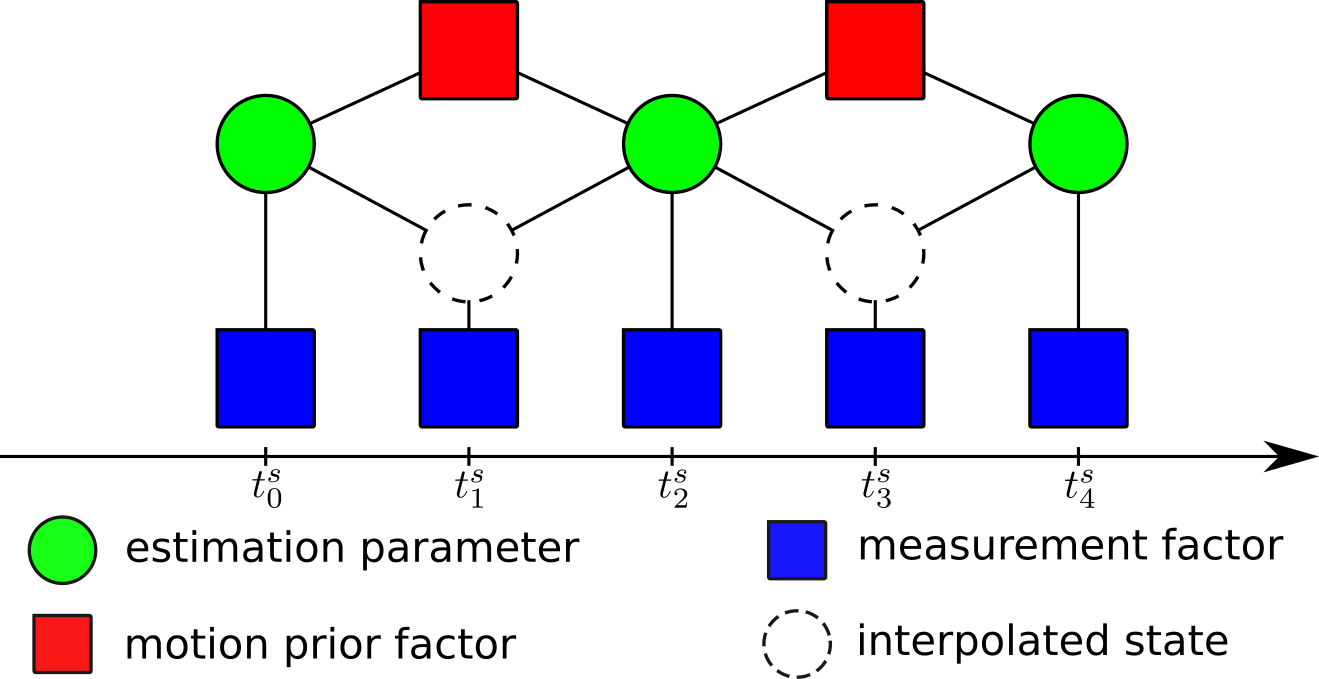
When performing estimation using GP regression, the states at the estimation times 𝐱¯n𝒳subscript¯𝐱𝑛𝒳\bar{\mathbf{x}}_{n}\in\mathcal{X} are the estimation parameters. It is usually preferable (although not necessary) to choose estimation times that correlate with a subset of the measurement times. Then, when evaluating residuals for these measurements, no state interpolation is necessary. However, it is often the case (e.g., when using high-frequency sensors) that there are too many measurements to associate a new estimation parameter with every measurement time. For measurement times that are not associated with an estimation parameter, the state is computed using the GP interpolation equation (21) (or the composition of equations (22), (15), (23), and (24) for Lie groups). The motion sample times {tj}superscriptsubscript𝑡𝑗\{t_{j}^{\prime}\} for the motion priors should coincide with the estimation times to avoid performing GP interpolation when evaluating them. Note that while the GP interpolation equation (21) is derived using a motion model, it is still possible to exclude the motion prior terms in (5) during estimation. We will refer to the inclusion (resp. exclusion) of these terms as “GP-based estimation with (resp. without) motion priors”. An example factor graph for GP-based estimation is shown in Figure 2.

In order to perform this estimation, we will need to compute the Jacobians of the interpolation equations as well as the motion priors with respect to the estimation parameters555For linear systems the interpolation function is linear, so these Jacobians are constant.. Unfortunately, we are only able to do this approximately for Lie groups. These Jacobians are derived in Appendix -C.
Refer to caption
Figure 2: An example factor graph for a GP-based estimator.

IV Spline-Based Estimation

Splines are piece-wise polynomial functions that are 𝒞k2superscript𝒞𝑘2\mathcal{C}^{k-2}-continuous (where k𝑘k is the spline order) at every point. They are an appealing way to model continuous trajectories because their evaluation at any point is only dependent on k𝑘k different parameters known as control points. The total number of control points used to represent the spline trajectory is a hyper-parameter that the user is able to specify. We first explain how splines are defined on vector spaces in Section IV-A, and then show how this definition can be extended to Lie groups in Section IV-B. Finally, we discuss how splines are used in continuous-time trajectory estimation problems in Section IV-C.

IV-A Vector Spaces

A spline of dimension d𝑑d and order k𝑘k is completely characterized by a set of control points {𝐩¯nd}n=1,,Nsubscriptsubscript¯𝐩𝑛superscript𝑑𝑛1𝑁\{\bar{\mathbf{p}}_{n}\in\mathbb{R}^{d}\}_{n=1,\cdots,N} and monotonically increasing knot points {tm}m=1,,N+ksubscriptsuperscriptsubscript𝑡𝑚𝑚1𝑁𝑘\{t_{m}^{\dagger}\in\mathbb{R}\}_{m=1,\cdots,N+k}. In our treatment, we will assume that the spacing between the knot points is uniform, i.e., tmtm1=δtmsuperscriptsubscript𝑡𝑚superscriptsubscript𝑡𝑚1𝛿𝑡for-all𝑚t_{m}^{\dagger}-t_{m-1}^{\dagger}=\delta t\ \forall\ m, for simplicity666It is possible to use non-uniform splines in estimation problems as well [39, 40, 41]. However, this adds an additional level of complexity and is beyond the scope of this paper.. The spline can be sampled at any point t[tk,tN+1]𝑡superscriptsubscript𝑡𝑘superscriptsubscript𝑡𝑁1t\in[t_{k}^{\dagger},t_{N+1}^{\dagger}] using

𝐩(t)=n=1NBn,k(t)𝐩¯n,𝐩𝑡superscriptsubscript𝑛1𝑁subscript𝐵𝑛𝑘𝑡subscript¯𝐩𝑛\mathbf{p}(t)=\sum_{n=1}^{N}B_{n,k}(t)\bar{\mathbf{p}}_{n}, (25)

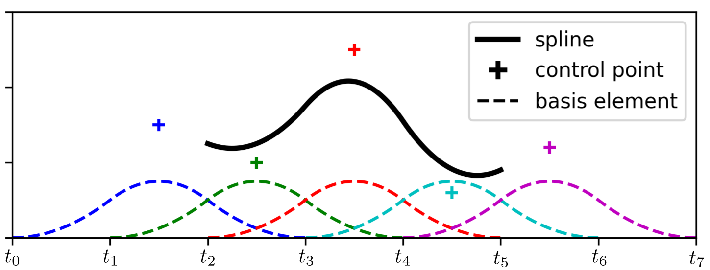
where Bn,k(t)subscript𝐵𝑛𝑘𝑡B_{n,k}(t) are the spline basis functions of order k𝑘k [14]. An example of a one-dimensional spline with k=3𝑘3k=3 is shown in Figure 3.

Refer to caption
Figure 3: One-dimensional spline example, with k=3𝑘3k=3.

While (25) is sufficient for spline evaluation, it requires evaluating all of the spline basis functions, only k𝑘k of which will be nonzero for any value of t𝑡t, and it is unwieldy to use in estimation problems. We can re-express (25) in a cumulative form

𝐩(t)=B~1,k(t)𝐩¯1+n=2MB~n,k(t)(𝐩¯n𝐩¯n1),𝐩𝑡subscript~𝐵1𝑘𝑡subscript¯𝐩1superscriptsubscript𝑛2𝑀subscript~𝐵𝑛𝑘𝑡subscript¯𝐩𝑛subscript¯𝐩𝑛1\mathbf{p}(t)=\tilde{B}_{1,k}(t)\bar{\mathbf{p}}_{1}+\sum_{n=2}^{M}\tilde{B}_{n,k}(t)(\bar{\mathbf{p}}_{n}-\bar{\mathbf{p}}_{n-1}), (26)

where B~n,k(t)=l=nMBl,k(t)subscript~𝐵𝑛𝑘𝑡superscriptsubscript𝑙𝑛𝑀subscript𝐵𝑙𝑘𝑡\tilde{B}_{n,k}(t)=\sum_{l=n}^{M}B_{l,k}(t). If we remove terms that evaluate to zero, we get

𝐩(t)=𝐩¯nk+1+j=1k1bj(u(t))(𝐩¯n+jk+1𝐩¯n+jk),𝐩𝑡subscript¯𝐩𝑛𝑘1superscriptsubscript𝑗1𝑘1subscript𝑏𝑗𝑢𝑡subscript¯𝐩𝑛𝑗𝑘1subscript¯𝐩𝑛𝑗𝑘\mathbf{p}(t)=\bar{\mathbf{p}}_{n-k+1}+\sum_{j=1}^{k-1}b_{j}(u(t))(\bar{\mathbf{p}}_{n+j-k+1}-\bar{\mathbf{p}}_{n+j-k}), (27)

where the index n𝑛n is chosen such that t(tn,tn+1]𝑡superscriptsubscript𝑡𝑛superscriptsubscript𝑡𝑛1t\in(t_{n}^{\dagger},t_{n+1}^{\dagger}], u(t)=ttntn+1tn(0,1]𝑢𝑡𝑡superscriptsubscript𝑡𝑛superscriptsubscript𝑡𝑛1superscriptsubscript𝑡𝑛01u(t)=\frac{t-t_{n}^{\dagger}}{t_{n+1}^{\dagger}-t_{n}^{\dagger}}\in(0,1], and bj(u)subscript𝑏𝑗𝑢b_{j}(u) is the j𝑗j-th element of 𝐛(u)=𝐂k𝝁(u)𝐛𝑢subscript𝐂𝑘𝝁𝑢\mathbf{b}(u)=\mathbf{C}_{k}\boldsymbol{\mu}(u), where 𝐂kk×ksubscript𝐂𝑘superscript𝑘𝑘\mathbf{C}_{k}\in\mathbb{R}^{k\times k} encodes the continuity constraints of the spline [42] and

𝝁(u)=[1u(t)u(t)2u(t)k1].𝝁𝑢superscriptmatrix1𝑢𝑡𝑢superscript𝑡2𝑢superscript𝑡𝑘1top\boldsymbol{\mu}(u)=\begin{bmatrix}1&u(t)&u(t)^{2}&\cdots&u(t)^{k-1}\end{bmatrix}^{\top}. (28)

Finally, we can rewrite (27) as

𝐩(t)=Θ(t)𝐩¯,𝐩𝑡Θ𝑡¯𝐩\mathbf{p}(t)=\Theta(t)\bar{\mathbf{p}}, (29)

where

Θ(t)=[(b0b1)𝐈(b1b2)𝐈bk1𝐈]Θ𝑡matrixsubscript𝑏0subscript𝑏1𝐈subscript𝑏1subscript𝑏2𝐈subscript𝑏𝑘1𝐈\Theta(t)=\begin{bmatrix}(b_{0}-b_{1})\mathbf{I}&(b_{1}-b_{2})\mathbf{I}&\cdots&b_{k-1}\mathbf{I}\end{bmatrix} (30)

(the dependence of bjsubscript𝑏𝑗b_{j} on u(t)𝑢𝑡u(t) has been omitted for brevity) and 𝐩¯=[𝐩¯nk+1𝐩¯nk+2𝐩¯n]¯𝐩superscriptmatrixsuperscriptsubscript¯𝐩𝑛𝑘1topsuperscriptsubscript¯𝐩𝑛𝑘2topsuperscriptsubscript¯𝐩𝑛toptop\bar{\mathbf{p}}=\begin{bmatrix}\bar{\mathbf{p}}_{n-k+1}^{\top}&\bar{\mathbf{p}}_{n-k+2}^{\top}&\cdots&\bar{\mathbf{p}}_{n}^{\top}\end{bmatrix}^{\top}. Computing time-derivatives of Euclidean B-splines is trivial with (29),

𝐩˙(t)=Θ˙(t)𝐩¯,𝐩¨(t)=Θ¨(t)𝐩¯,.formulae-sequence˙𝐩𝑡˙Θ𝑡¯𝐩¨𝐩𝑡¨Θ𝑡¯𝐩\dot{\mathbf{p}}(t)=\dot{\Theta}(t)\bar{\mathbf{p}},\quad\ddot{\mathbf{p}}(t)=\ddot{\Theta}(t)\bar{\mathbf{p}},\quad\cdots. (31)

IV-B Lie Groups

It is possible to extend this representation of vector space splines to matrix Lie groups. We begin with the cumulative representation (27). Recall that the vector space dsuperscript𝑑\mathbb{R}^{d} is itself a Lie group, where the group operation is vector addition, inversion is vector negation, and the exponential and logarithmic maps are identity. We can generalize (27) to any Lie group by substituting these operations. Let G𝐺G be an arbitrary Lie group with Lie algebra 𝔤𝔤\mathfrak{g} and dimension d𝑑d, and let {g¯nG}n=1,,Nsubscriptsubscript¯𝑔𝑛𝐺𝑛1𝑁\{\bar{g}_{n}\in G\}_{n=1,\cdots,N} be a set of control points. Then a spline on G𝐺G can be sampled at the point t𝑡t using

g(t)=g¯nk+1j=1MExp(bj(u(t))𝛀n+jk+1),𝛀i=Log(g¯i11g¯i).formulae-sequence𝑔𝑡subscript¯𝑔𝑛𝑘1superscriptsubscriptproduct𝑗1𝑀Expsubscript𝑏𝑗𝑢𝑡subscript𝛀𝑛𝑗𝑘1subscript𝛀𝑖Logsuperscriptsubscript¯𝑔𝑖11subscript¯𝑔𝑖\begin{gathered}g(t)=\bar{g}_{n-k+1}\prod_{j=1}^{M}\text{Exp}\left(b_{j}(u(t))\boldsymbol{\Omega}_{n+j-k+1}\right),\\ \boldsymbol{\Omega}_{i}=\text{Log}(\bar{g}_{i-1}^{-1}\bar{g}_{i}).\end{gathered} (32)

This can be understood as taking products of scaled geodesics between consecutive control points. Note that (27) and (32) are identical for the specific Lie group dsuperscript𝑑\mathbb{R}^{d}.

We will need to compute time derivatives g˙(t),g¨(t)d˙𝑔𝑡¨𝑔𝑡superscript𝑑\dot{g}(t),\ddot{g}(t)\in\mathbb{R}^{d} of (32) (which represent the same quantities as those in Section II-A2). This process is much more complicated than it was for vector space splines (31). We show how to compute the first two time derivatives in Appendix -D.

IV-C Estimation

When performing estimation using splines, the control points are usually defined on the configuration manifold \mathcal{M} of the system rather than on the state space 𝒳𝒳\mathcal{X}. Let the state of the system be 𝐱(t)={g(t),g˙(t),g¨(t),}×d×d×=𝒳𝐱𝑡𝑔𝑡˙𝑔𝑡¨𝑔𝑡superscript𝑑superscript𝑑𝒳\mathbf{x}(t)=\{g(t),\dot{g}(t),\ddot{g}(t),\cdots\}\in\mathcal{M}\times\mathbb{R}^{d}\times\mathbb{R}^{d}\times\cdots=\mathcal{X}. The state interpolation function (3) for splines is then computed using (29) and (31) for vector space splines or (32) and its derivatives in Appendix -D for Lie group splines.

As opposed to the GP formulation, splines are not directly motivated by a specific dynamic model. However, it is still possible to assume that the motion of the system obeys one of the models in Section II-A and to constrain the spline using the motion priors (11), (18). We have chosen to use these motion priors rather than those derived in [12] in order to more directly compare splines with GPs.

There is not an obvious way to choose the motion sample times {tj}superscriptsubscript𝑡𝑗\{t_{j}^{\prime}\} to ensure that the control points are fully constrained. In our analysis for vector space splines in Section VI, we will show the effect that the motion sample period δt=tjtj1𝛿superscript𝑡superscriptsubscript𝑡𝑗superscriptsubscript𝑡𝑗1\delta t^{\prime}=t_{j}^{\prime}-t_{j-1}^{\prime} has on estimation results. An example factor graph for spline-based estimation with k=3𝑘3k=3 is given in Figure 4.

To perform estimation using splines, we will need to compute the Jacobians of the interpolation function with respect to the control points777In the case of vector space splines, the interpolation function is linear, so these Jacobians are constant.. These Jacobians are derived in Appendix -E.
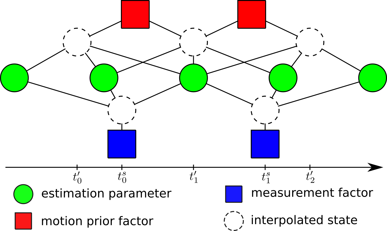
Refer to caption
Figure 4: Example factor graph for a spline-based estimator with k=3𝑘3k=3. Note the relative sparsity between this graph and the general graph in Figure 1.

V Estimation Scenarios

We aim to compare GP-based estimation against spline-based estimation in a couple of scenarios. Our first scenario is a simple linear model introduced in Section V-A. This will allow us to understand how the various hyper-parameters of each estimation scheme affect the estimated solution at a high level. Next, we will look at a more complicated system that fuses low frequency fiducial pose measurements obtained from a monocular camera with high frequency IMU measurements. The configuration manifold of the camera is the Lie group SE(3). This will allow us to compare the GP and spline Lie group adaptations directly. This scenario is introduced in Section V-B.

V-A Linear Estimation

Let the state of a linear system be 𝐱(t)=[d(t)v(t)a(t)]𝐱𝑡superscriptmatrix𝑑superscript𝑡top𝑣superscript𝑡top𝑎superscript𝑡toptop\mathbf{x}(t)=\begin{bmatrix}d(t)^{\top}&v(t)^{\top}&a(t)^{\top}\end{bmatrix}^{\top}, where d(t),v(t),a(t)2𝑑𝑡𝑣𝑡𝑎𝑡superscript2d(t),v(t),a(t)\in\mathbb{R}^{2} are respectively the position, velocity, and acceleration of the system, and assume that it evolves according to

𝐱˙(t)=[𝟎𝐈𝟎𝟎𝟎𝐈𝟎𝟎𝟎]𝐱(t)+[𝟎𝟎𝐈]𝐰(t)˙𝐱𝑡matrix0𝐈000𝐈000𝐱𝑡matrix00𝐈𝐰𝑡\dot{\mathbf{x}}(t)=\begin{bmatrix}\mathbf{0}&\mathbf{I}&\mathbf{0}\\ \mathbf{0}&\mathbf{0}&\mathbf{I}\\ \mathbf{0}&\mathbf{0}&\mathbf{0}\end{bmatrix}\mathbf{x}(t)+\begin{bmatrix}\mathbf{0}\\ \mathbf{0}\\ \mathbf{I}\end{bmatrix}\mathbf{w}(t) (33)

(i.e., a WNOJ model), where 𝐰(t)𝒢𝒫(𝟎,δ(tt)𝐐)similar-to𝐰𝑡𝒢𝒫0𝛿𝑡superscript𝑡𝐐\mathbf{w}(t)\sim\mathcal{GP}(\mathbf{0},\delta(t-t^{\prime})\mathbf{Q}). The system receives measurements

𝐳is=d(tis)+𝜼,superscriptsubscript𝐳𝑖𝑠𝑑superscriptsubscript𝑡𝑖𝑠𝜼\mathbf{z}_{i}^{s}=d(t_{i}^{s})+\boldsymbol{\eta}, (34)

where tissuperscriptsubscript𝑡𝑖𝑠t_{i}^{s} is the measurement time and 𝜼𝒩(𝟎,𝐑)similar-to𝜼𝒩0𝐑\boldsymbol{\eta}\sim\mathcal{N}(\mathbf{0},\mathbf{R}) is zero-mean Gaussian noise with covariance 𝐑𝐑\mathbf{R}. Because the measurement function and the system are both linear and defined on a vector space, the estimation problem (5) can be solved analytically using linear least squares for both GPs and splines. In Section VI we will provide an in-depth comparison between the performance of GP-based and spline-based estimation for this system.

V-B Camera and IMU Estimation

Let the pose of an IMU be 𝐓(t)SE(3)superscriptsubscript𝐓𝑡SE3\mathbf{T}_{\mathcal{I}}^{\mathcal{B}}(t)\in\text{SE}(3), where \mathcal{I} represents an inertial coordinate frame, \mathcal{B} represents the IMU coordinate frame, and 𝐓superscriptsubscript𝐓\mathbf{T}_{\mathcal{I}}^{\mathcal{B}} is the homogeneous transformation from \mathcal{I} to \mathcal{B}. The IMU pose has dynamics

𝐓˙(t)=ϖ/(t)𝐓(t),ϖ˙/(t)=𝜶/(t),𝜶˙/(t)=𝐰(t),formulae-sequencesuperscriptsubscript˙𝐓𝑡superscriptsubscriptbold-italic-ϖsuperscript𝑡superscriptsubscript𝐓𝑡formulae-sequencesuperscriptsubscript˙bold-italic-ϖ𝑡superscriptsubscript𝜶𝑡superscriptsubscript˙𝜶𝑡𝐰𝑡\begin{gathered}\dot{\mathbf{T}}_{\mathcal{I}}^{\mathcal{B}}(t)=-\boldsymbol{\varpi}_{\mathcal{B}/\mathcal{I}}^{\mathcal{B}}(t)^{\wedge}\mathbf{T}_{\mathcal{I}}^{\mathcal{B}}(t),\\ \dot{\boldsymbol{\varpi}}_{\mathcal{B}/\mathcal{I}}^{\mathcal{B}}(t)=\boldsymbol{\alpha}_{\mathcal{B}/\mathcal{I}}^{\mathcal{B}}(t),\\ \dot{\boldsymbol{\alpha}}_{\mathcal{B}/\mathcal{I}}^{\mathcal{B}}(t)=\mathbf{w}(t),\end{gathered} (35)

where ϖ/=[𝐯/𝝎/]6superscriptsubscriptbold-italic-ϖsuperscriptmatrixsuperscriptsubscript𝐯superscripttopsuperscriptsubscript𝝎superscripttoptopsuperscript6\boldsymbol{\varpi}_{\mathcal{B}/\mathcal{I}}^{\mathcal{B}}=\begin{bmatrix}{\mathbf{v}_{\mathcal{B}/\mathcal{I}}^{\mathcal{B}^{\top}}}&{\boldsymbol{\omega}_{\mathcal{B}/\mathcal{I}}^{\mathcal{B}^{\top}}}\end{bmatrix}^{\top}\in\mathbb{R}^{6} is the twist of the IMU with velocity 𝐯/superscriptsubscript𝐯\mathbf{v}_{\mathcal{B}/\mathcal{I}}^{\mathcal{B}} and angular velocity 𝝎/superscriptsubscript𝝎\boldsymbol{\omega}_{\mathcal{B}/\mathcal{I}}^{\mathcal{B}}, and where 𝜶/=[𝐚/𝝎˙/]6superscriptsubscript𝜶superscriptmatrixsuperscriptsubscript𝐚superscripttopsuperscriptsubscript˙𝝎superscripttoptopsuperscript6\boldsymbol{\alpha}_{\mathcal{B}/\mathcal{I}}^{\mathcal{B}}=\begin{bmatrix}{\mathbf{a}_{\mathcal{B}/\mathcal{I}}^{\mathcal{B}^{\top}}}&{\dot{\boldsymbol{\omega}}_{\mathcal{B}/\mathcal{I}}^{\mathcal{B}^{\top}}}\end{bmatrix}^{\top}\in\mathbb{R}^{6} with acceleration 𝐚/superscriptsubscript𝐚\mathbf{a}_{\mathcal{B}/\mathcal{I}}^{\mathcal{B}}, and 𝐰(t)𝒢𝒫(𝟎,δ(tt)𝐐)similar-to𝐰𝑡𝒢𝒫0𝛿𝑡superscript𝑡𝐐\mathbf{w}(t)\sim\mathcal{GP}(\mathbf{0},\delta(t-t^{\prime})\mathbf{Q}).

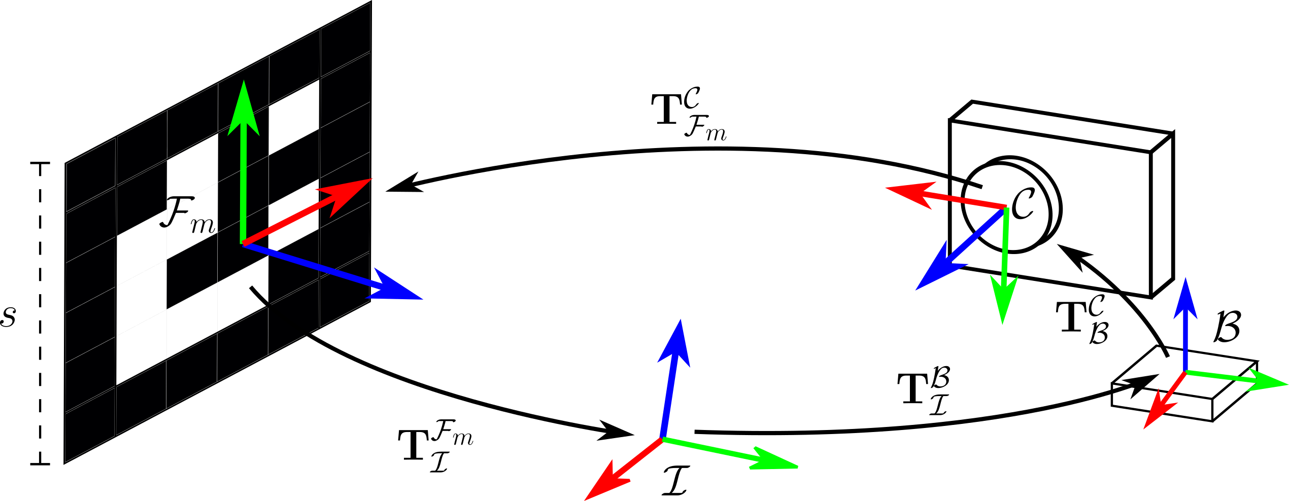
Additionally, there is a monocular camera with coordinate frame 𝒞𝒞\mathcal{C} that is rigidly attached to the IMU with precalibrated relative transformation 𝐓𝒞SE(3)superscriptsubscript𝐓𝒞SE3\mathbf{T}_{\mathcal{B}}^{\mathcal{C}}\in\text{SE}(3). The camera views fiducial markers with coordinate frames m,m=1,,Mformulae-sequencesubscript𝑚𝑚1𝑀\mathcal{F}_{m},m=1,\cdots,M and known inertial poses 𝐓msuperscriptsubscript𝐓subscript𝑚\mathbf{T}_{\mathcal{I}}^{\mathcal{F}_{m}} and, using the Perspective-N-Point (PnP) algorithm [43], finds the relative pose between the marker and the camera 𝐓m𝒞superscriptsubscript𝐓subscript𝑚𝒞\mathbf{T}_{\mathcal{F}_{m}}^{\mathcal{C}}. This scenario is depicted in Figure 5.
Refer to caption
Figure 5: Relevant coordinate frames for the camera and IMU scenario.

The measurement models for the gyroscope and accelerometer are

𝐳ig=𝝎/(tig)+𝐛g+𝜼gsuperscriptsubscript𝐳𝑖𝑔superscriptsubscript𝝎superscriptsubscript𝑡𝑖𝑔superscript𝐛𝑔superscript𝜼𝑔\mathbf{z}_{i}^{g}=\boldsymbol{\omega}_{\mathcal{B}/\mathcal{I}}^{\mathcal{B}}(t_{i}^{g})+\mathbf{b}^{g}+\boldsymbol{\eta}^{g} (36)

and

𝐳ia=𝐚/(tia)g𝐑(tia)𝐞3+𝐛a+𝜼a,superscriptsubscript𝐳𝑖𝑎superscriptsubscript𝐚superscriptsubscript𝑡𝑖𝑎𝑔superscriptsubscript𝐑superscriptsubscript𝑡𝑖𝑎subscript𝐞3superscript𝐛𝑎superscript𝜼𝑎\mathbf{z}_{i}^{a}=\mathbf{a}_{\mathcal{B}/\mathcal{I}}^{\mathcal{B}}(t_{i}^{a})-g\mathbf{R}_{\mathcal{I}}^{\mathcal{B}}(t_{i}^{a})\mathbf{e}_{3}+\mathbf{b}^{a}+\boldsymbol{\eta}^{a}, (37)

respectively, where tigsuperscriptsubscript𝑡𝑖𝑔t_{i}^{g} and tiasuperscriptsubscript𝑡𝑖𝑎t_{i}^{a} are the measurement timestamps, 𝜼g𝒩(𝟎,𝚺g)similar-tosuperscript𝜼𝑔𝒩0superscript𝚺𝑔\boldsymbol{\eta}^{g}\sim\mathcal{N}(\mathbf{0},\boldsymbol{\Sigma}^{g}) and 𝜼a𝒩(𝟎,𝚺a)similar-tosuperscript𝜼𝑎𝒩0superscript𝚺𝑎\boldsymbol{\eta}^{a}\sim\mathcal{N}(\mathbf{0},\boldsymbol{\Sigma}^{a}) are additive Gaussian noise with covariance 𝚺gsuperscript𝚺𝑔\boldsymbol{\Sigma}^{g} and 𝚺asuperscript𝚺𝑎\boldsymbol{\Sigma}^{a} respectively, 𝐛g,𝐛a3superscript𝐛𝑔superscript𝐛𝑎superscript3\mathbf{b}^{g},\mathbf{b}^{a}\in\mathbb{R}^{3} are walking bias terms with dynamics

𝐛˙g=𝜼bg,𝐛˙a=𝜼ba,formulae-sequencesuperscript˙𝐛𝑔superscript𝜼𝑏𝑔superscript˙𝐛𝑎superscript𝜼𝑏𝑎\dot{\mathbf{b}}^{g}=\boldsymbol{\eta}^{bg},\quad\dot{\mathbf{b}}^{a}=\boldsymbol{\eta}^{ba}, (38)

where 𝜼bg𝒩(𝟎,𝚺bg),𝜼ba𝒩(𝟎,𝚺ba)formulae-sequencesimilar-tosuperscript𝜼𝑏𝑔𝒩0superscript𝚺𝑏𝑔similar-tosuperscript𝜼𝑏𝑎𝒩0superscript𝚺𝑏𝑎\boldsymbol{\eta}^{bg}\sim\mathcal{N}(\mathbf{0},\boldsymbol{\Sigma}^{bg}),\ \boldsymbol{\eta}^{ba}\sim\mathcal{N}(\mathbf{0},\boldsymbol{\Sigma}^{ba}), and where g𝑔g is the constant of gravitational acceleration. The fiducial pose measurement model is

𝐳imc=Exp(𝜼c)𝐓𝒞𝐓(timc)𝐓m1,superscriptsubscript𝐳subscript𝑖𝑚𝑐Expsuperscript𝜼𝑐superscriptsubscript𝐓𝒞superscriptsubscript𝐓superscriptsubscript𝑡subscript𝑖𝑚𝑐superscriptsuperscriptsubscript𝐓subscript𝑚1\mathbf{z}_{i_{m}}^{c}=\text{Exp}(\boldsymbol{\eta}^{c})\mathbf{T}_{\mathcal{B}}^{\mathcal{C}}\mathbf{T}_{\mathcal{I}}^{\mathcal{B}}(t_{i_{m}}^{c}){\mathbf{T}_{\mathcal{I}}^{\mathcal{F}_{m}}}^{-1}, (39)

where timcsuperscriptsubscript𝑡subscript𝑖𝑚𝑐t_{i_{m}}^{c} is the measurement timestamp and 𝜼𝒄𝒩(𝟎,𝚺c)similar-tosuperscript𝜼𝒄𝒩0superscript𝚺𝑐\boldsymbol{\eta^{c}}\sim\mathcal{N}(\mathbf{0},\boldsymbol{\Sigma}^{c}). The fiducial pose covariance 𝚺csuperscript𝚺𝑐\boldsymbol{\Sigma}^{c} varies depending on the viewing angle and distance. We compute it for each individual measurement by propagating the pixel projection covariance 𝚺p2×2superscript𝚺𝑝superscript22\boldsymbol{\Sigma}^{p}\in\mathbb{R}^{2\times 2} through the PnP model using the fiducial side length s𝑠s and the camera projection matrix 𝐊3×3𝐊superscript33\mathbf{K}\in\mathbb{R}^{3\times 3}.

The dynamic state of this system resides in the Lie group SE(3), so it will be necessary to use a Lie group GP or a Lie group spline to solve this problem. We provide in-depth comparisons for these two estimation methods using simulated measurements and real measurements in Sections VII and VIII, respectively.

VI Linear Simulation Comparison

For our linear simulation comparison, we implemented the system in Section V-A with the following parameters:

𝐐=[1.0000.01](m/s3)2,𝐑=0.012𝐈m2.formulae-sequence𝐐matrix1.0000.01superscriptmsuperscripts32𝐑superscript0.012𝐈superscriptm2\mathbf{Q}=\begin{bmatrix}1.0&0\\ 0&0.01\end{bmatrix}$\mathrm{(}\mathrm{m}\mathrm{/}\mathrm{s}^{3}\mathrm{)}^{2}$,\quad\mathbf{R}=0.01^{2}\mathbf{I}\>$\mathrm{m}^{2}$. (40)

Measurements were simulated at 100 HzHz\mathrm{H}\mathrm{z} for 20 ss\mathrm{s} with initial conditions d(t0)=𝟎𝑑subscript𝑡00d(t_{0})=\mathbf{0} mm\mathrm{m}, v(t0)=[1.0,0.0]𝑣subscript𝑡0superscriptmatrix1.00.0topv(t_{0})=\begin{bmatrix}1.0,0.0\end{bmatrix}^{\top} m/sms\mathrm{m}\mathrm{/}\mathrm{s}, and a(t0)=𝟎𝑎subscript𝑡00a(t_{0})=\mathbf{0} m/s2msuperscripts2\mathrm{m}\mathrm{/}\mathrm{s}^{2}.

Refer to caption
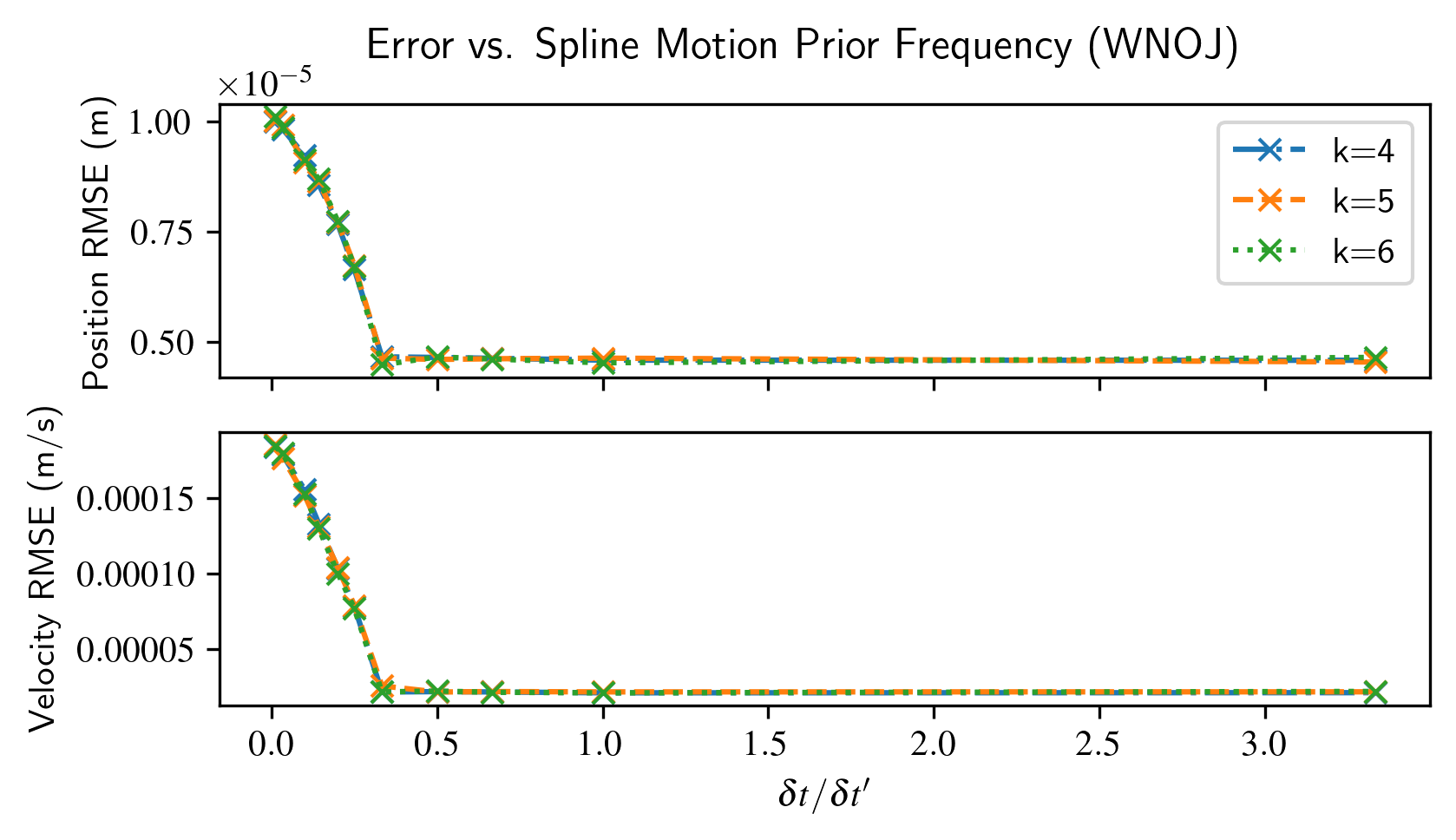
Figure 6: Spline-based trajectory error versus spline motion prior frequency for several values of k𝑘k. Both the trajectory and motion priors used a WNOJ model. The values shown are the medians over 50 Monte Carlo trials.

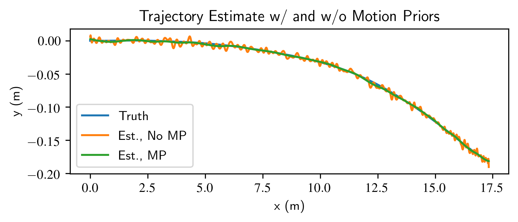
We wish to compare the performance of GP-based estimation to spline-based estimation for this scenario. In order to do this, we first need to know how to select the spline motion sample period δt𝛿superscript𝑡\delta t^{\prime} to fully constrain the motion of the system. Figure 6 shows the position and velocity root-mean-square-error (RMSE) for the spline trajectory estimate for varying values of the spline order k𝑘k and the ratio between the knot period δt𝛿𝑡\delta t and δt𝛿superscript𝑡\delta t^{\prime}. The values shown are the medians over 50 Monte Carlo trials. As can be seen, the RMSE stops improving as soon as δt/δt=13𝛿𝑡𝛿superscript𝑡13\delta t/\delta t^{\prime}=\frac{1}{3}, showing that the motion is fully constrained at this value. This ratio means that there is one motion prior for every three control points. This makes sense because each WNOJ motion prior introduces three constraints on 𝐱(t)𝐱𝑡\mathbf{x}(t), so the number of constraints and control points is one-to-one. Figure 7 qualitatively shows the effect that the motion priors have on the trajectory estimate.
Refer to caption
Figure 7: Spline-based trajectory estimation with and without motion priors.

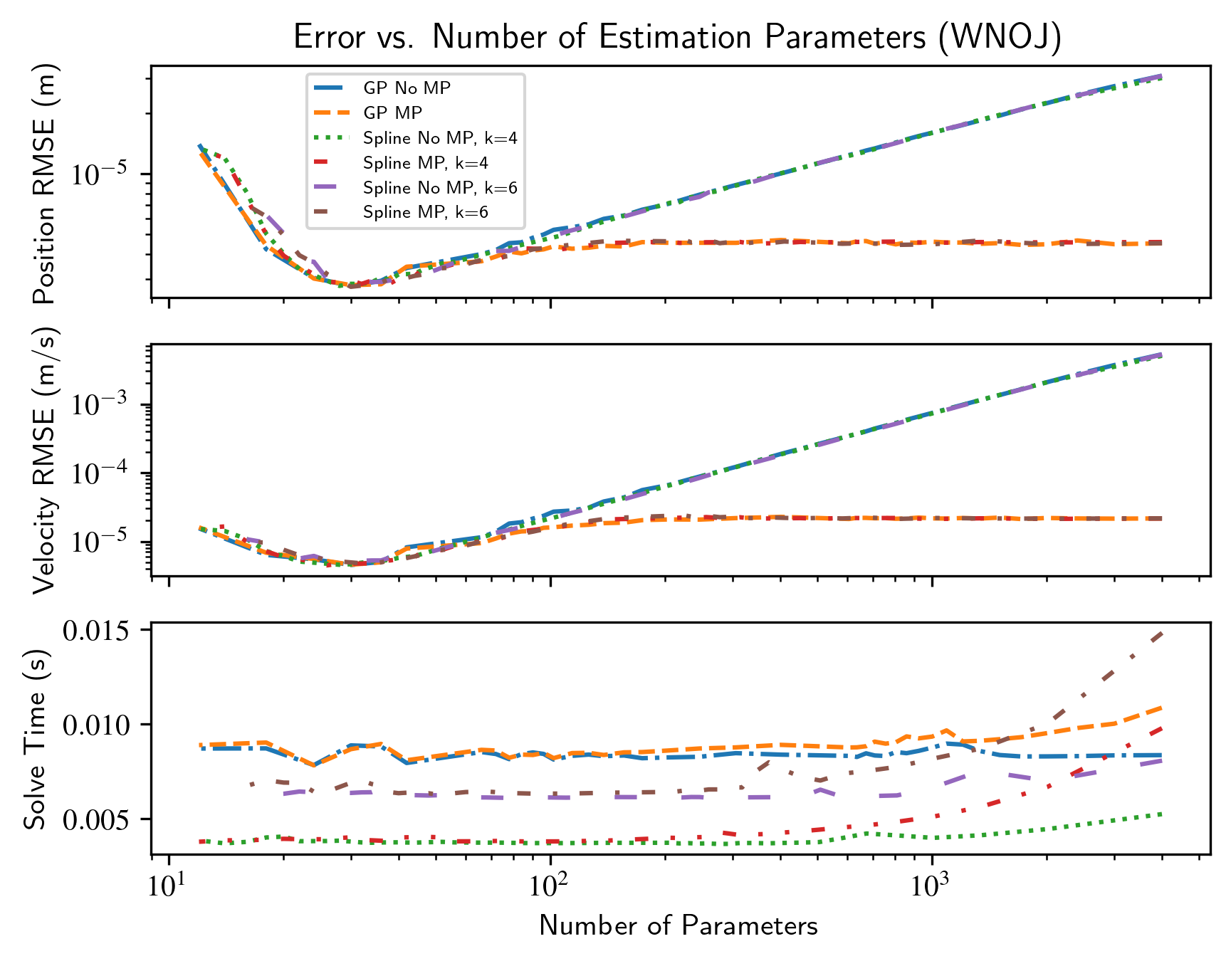
With this knowledge in hand, we performed GP-based and spline-based estimation for varying values of k𝑘k, δt𝛿𝑡\delta t, and nGPsubscript𝑛GPn_{\text{GP}}, where nGPsubscript𝑛GPn_{\text{GP}} means that a GP estimation parameter was placed at every nGPsubscript𝑛GPn_{\text{GP}}-th measurement time. We compared each method with and without motion priors to show the effect that the cost terms (11) have on the solution and to determine if one of the methods is less prone to over-fitting measurement noise when no regularization is present. The value of δt𝛿superscript𝑡\delta t^{\prime} was chosen such that δt/δt=13𝛿𝑡𝛿superscript𝑡13\delta t/\delta t^{\prime}=\frac{1}{3}, and the GP estimator placed one motion prior between each consecutive set of estimation times. The results are shown in Figure 8. The horizontal axis shows the total number of floating point values used in the estimation parameters, and the vertical axes show the position RMSE, velocity RMSE, and solve time888Note that because the system model is linear and Euclidean, the estimation problem has an analytic solution for both splines and GPs. The solve times shown indicate the amount of compute time required to solve the linear system of equations via sparse Cholesky decomposition.. Without motion priors, the RMSE increased as the number of parameters increased for both GPs and splines, indicating that the estimated trajectories overfit the measurement noise. When motion priors were used, the error leveled out as the number of parameters increased, meaning that the priors prevented the trajectory from fitting the measurement noise999Note the slight increase in trajectory RMSE in Figure 8 before leveling out as the number of parameters increases when using motion priors. This behavior is caused by the relative weighting in the motion prior terms versus the measurement terms in (5). When a low number of parameters are used, the time between parameters is large and the inverse covariance 𝐐tj+11superscriptsubscript𝐐subscriptsuperscript𝑡𝑗11\mathbf{Q}_{t^{\prime}_{j+1}}^{-1} is significantly smaller than 𝚺s1superscriptsubscript𝚺𝑠1\boldsymbol{\Sigma}_{s}^{-1}, thus the motion priors have little to no effect on the solution. As the number of parameters increases the effect of the motion priors becomes more significant. In the case of Figure 8, the trajectory has enough freedom to fit the measurement noise slightly before the cost of the motion prior terms becomes significant compared to the cost of the measurement terms.. It is especially interesting to note that the trajectory errors are approximately equivalent for GPs and splines regardless of the number of parameters used or the value of the spline order k𝑘k. The solve time tended to increase with the number of estimation parameters, especially when using motion priors. The spline estimate for k=6𝑘6k=6 using motion priors had the longest solve time, likely because the time complexity of the spline interpolation equation (29) is linear in k𝑘k. However, the increase in order did not provide superior performance in this case, thus it seems that picking a lower value for k𝑘k would be reasonable.

Refer to caption
Figure 8: Trajectory error and solve time versus number of floating point estimation parameters for a WNOJ trajectory, for both splines and GPs with and without motion priors. The values shown are the medians over 50 Monte Carlo trials.

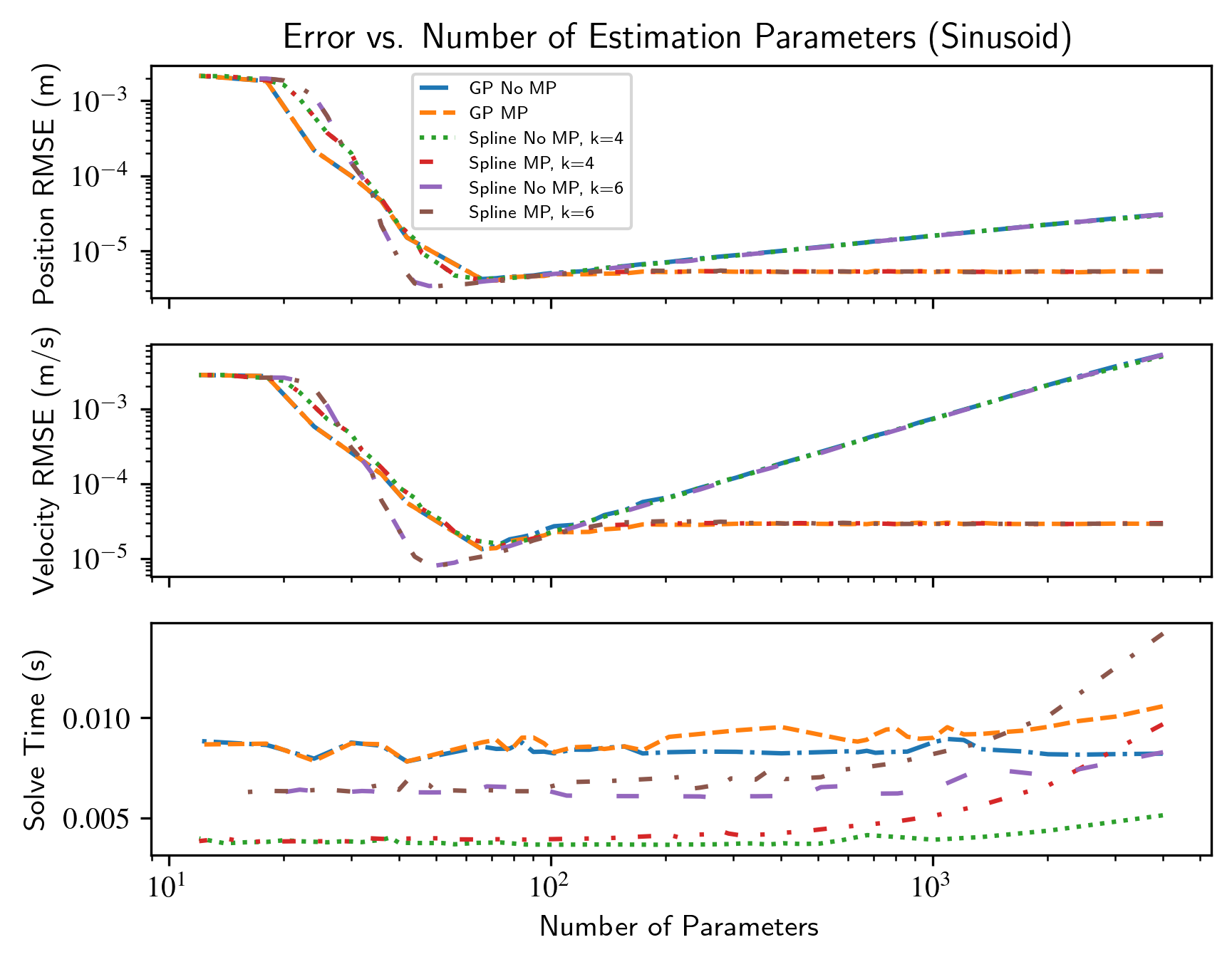
In addition to WNOJ trajectories, we simulated a circular sinusoidal trajectory in order to show the performance of the two estimation methods when the assumed motion model does not perfectly match the true motion of the system. We used WNOJ motion priors and chose 𝐐=𝐈(m/s3)2𝐐𝐈superscriptmsuperscripts32\mathbf{Q}=\mathbf{I}$\mathrm{(}\mathrm{m}\mathrm{/}\mathrm{s}^{3}\mathrm{)}^{2}$. The results are shown in Figure 9. When motion priors were not used, the error decreased at first as the number of estimation parameters increased, and then increased when the estimated trajectory began to fit the measurement noise. When using motion priors, the error decreased in a similar manner, but then leveled out, indicating that the motion priors restricted the trajectory from overfitting the measurements. Once again, GPs and splines had similar accuracy, regardless of the number of parameters used or the value of k𝑘k. The solve time followed a similar trend to the previous experiment.
Refer to caption
Figure 9: Trajectory error and solve time versus number of floating point estimation parameters for a sinusoidal trajectory, for both splines and GPs with and without motion priors. The motion priors use a WNOJ model. The values shown are the medians over 50 Monte Carlo trials.,

VII IMU Simulation Comparison

We additionally simulated the camera and IMU scenario described in Section V-B. The following parameters were used:

𝐓𝒞=[𝐈𝐩/𝒞𝒞𝟎1],𝐩/𝒞𝒞=[0.00.00.1]m𝐐=[5.0𝐈𝟎𝟎1.5𝐈],𝚺g=σg2𝐈,σg=0.005rad/s𝚺a=σa2𝐈,σa=0.005m/s2,𝚺bg=σbg2𝐈,σbg=0.005rad/s2,𝚺ba=σba2𝐈,σba=0.005m/s3.\begin{gathered}\mathbf{T}_{\mathcal{B}}^{\mathcal{C}}=\begin{bmatrix}\mathbf{I}&\mathbf{p}_{\mathcal{B}/\mathcal{C}}^{\mathcal{C}}\\ \mathbf{0}&1\end{bmatrix},\quad\mathbf{p}_{\mathcal{B}/\mathcal{C}}^{\mathcal{C}}=\begin{bmatrix}0.0\\ 0.0\\ 0.1\end{bmatrix}~{}$\mathrm{m}$\\ \mathbf{Q}=\begin{bmatrix}5.0\mathbf{I}&\mathbf{0}\\ \mathbf{0}&1.5\mathbf{I}\end{bmatrix},\quad\boldsymbol{\Sigma}_{g}=\sigma_{g}^{2}\mathbf{I},\quad\sigma_{g}=0.005~{}$\mathrm{r}\mathrm{a}\mathrm{d}\mathrm{/}\mathrm{s}$\\ \boldsymbol{\Sigma}_{a}=\sigma_{a}^{2}\mathbf{I},\quad\sigma_{a}=0.005~{}$\mathrm{m}\mathrm{/}\mathrm{s}^{2}$,\\ \boldsymbol{\Sigma}_{bg}=\sigma_{bg}^{2}\mathbf{I},\quad\sigma_{bg}=0.005~{}$\mathrm{r}\mathrm{a}\mathrm{d}\mathrm{/}\mathrm{s}^{2}$,\\ \boldsymbol{\Sigma}_{ba}=\sigma_{ba}^{2}\mathbf{I},\quad\sigma_{ba}=0.005~{}$\mathrm{m}\mathrm{/}\mathrm{s}^{3}$.\end{gathered} (41)

We placed a single fiducial marker at the origin of the inertial frame. When simulating fiducial pose measurements from the camera, we either used a constant pose covariance

𝚺c=0.05𝐈subscript𝚺𝑐0.05𝐈\boldsymbol{\Sigma}_{c}=0.05\mathbf{I} (42)

or we simulated the way noise from the camera propagates to the PnP solution using

𝚺p=σp2𝐈,σp=0.5px,𝐊=[fx0cx0fycy001],fx=fy=620px,cx=320px,cy=240px,s=0.4m.\begin{gathered}\boldsymbol{\Sigma}_{p}=\sigma_{p}^{2}\mathbf{I},\quad\sigma_{p}=0.5~{}$\mathrm{p}\mathrm{x}$,\\ \mathbf{K}=\begin{bmatrix}f_{x}&0&c_{x}\\ 0&f_{y}&c_{y}\\ 0&0&1\end{bmatrix},\quad f_{x}=f_{y}=620~{}$\mathrm{p}\mathrm{x}$,\\ c_{x}=320~{}$\mathrm{p}\mathrm{x}$,\quad c_{y}=240~{}$\mathrm{p}\mathrm{x}$,\quad s=0.4~{}$\mathrm{m}$.\end{gathered} (43)

When the camera trajectory was constrained such that the fiducial marker stayed in the field-of-view (FOV) of the simulated camera, the variable pose covariance was used. Otherwise the constant pose covariance was used, and pose measurements were simulated regardless of whether the fiducial marker was in the FOV. The camera was simulated at 10 HzHz\mathrm{H}\mathrm{z} and the IMU was simulated at 100 HzHz\mathrm{H}\mathrm{z}.

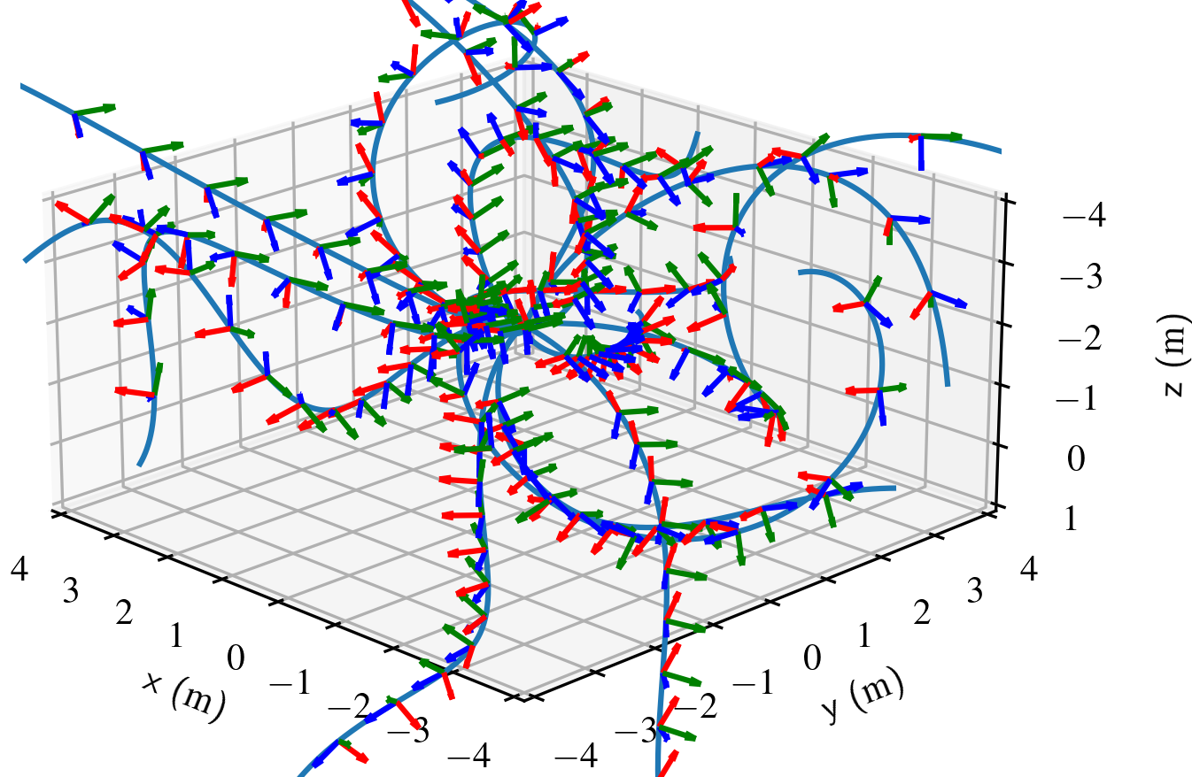
We simulated 10 ss\mathrm{s} WNOJ trajectories using the model in (35). A collection of these WNOJ trajectories is shown in Figure 10. Because these trajectories were not constrained to have the fiducial marker be in the camera FOV, the constant pose covariance model was used when simulating pose measurements.
Refer to caption
Figure 10: A collection of random WNOJ trajectories on SE(3).

We tested the ability of six different continuous-time trajectory representations to estimate the camera trajectory from the acquired fiducial pose measurements: splines on SE(3) with k=4𝑘4k=4 and k=6𝑘6k=6, GPs on SE(3), splines on SO(3)×3absentsuperscript3\times\mathbb{R}^{3} with k=4𝑘4k=4 and k=6𝑘6k=6, and GPs on SO(3)×3absentsuperscript3\times\mathbb{R}^{3}. When estimating on SO(3)×3absentsuperscript3\times\mathbb{R}^{3}, the translation and rotation were represented using separate splines or GPs. We included these representations in our analysis because previous works have found that decoupling rotation and translation in the estimation process can improve computational performance [44]. In addition, we varied the type of trajectory regularization that was used during estimation: motion priors, IMU measurements, both, or neither. When including IMU and/or motion priors, we ran estimation in two steps, first without regularization and then with regularization. This is because the estimator struggled to converge with poor initial conditions when including IMU or motion prior residuals. All estimation parameters were initialized to zero or identity. In all cases IMU biases were estimated as constant values (this is reasonable because the time window is relatively short). We used Levenberg-Marquardt optimization implemented with the Ceres Solver [45].

When including motion priors with spline-based estimation, we set the motion prior period δt𝛿superscript𝑡\delta t^{\prime} to three times the knot point period δt𝛿𝑡\delta t to be consistent with our findings in Section VI. Rather than vary the number of estimation parameters, we chose fixed values for the knot point period δt=0.1s𝛿𝑡0.1s\delta t=0.1~{}$\mathrm{s}$ and GP estimation frequency nGP=1subscript𝑛GP1n_{\text{GP}}=1 (meaning that an estimation time was placed at every nGPsubscript𝑛GPn_{\text{GP}}-th fiducial pose measurement). We found that these values provided accurate and consistent results for each of our test scenarios.

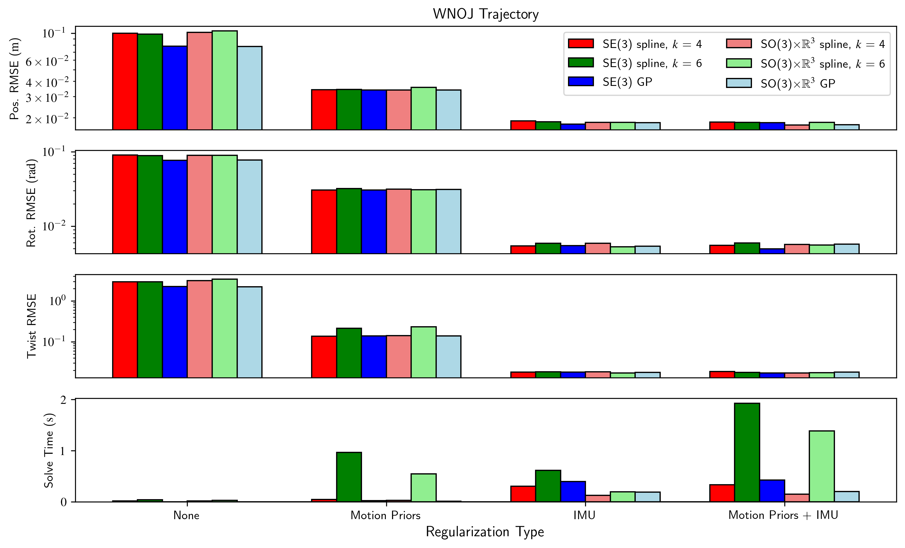
In each of these scenarios, we ran 100 Monte Carlo trials. The median pose, velocity, and twist RMSE, as well as the computation times for each of these scenarios are shown in Figure 11. There are several observations that can be made from this figure. First, all trajectory representations had better accuracy when including motion priors, and the best trajectory accuracy was achieved when using IMU measurements. Using motion priors in addition to the IMU measurements did not improve accuracy. We also note that when using the same type of regularization, each method achieved similar trajectory accuracy. The only exception is that the GP representations appear to have slightly lower error when no regularization is used, although the difference is not overly significant.

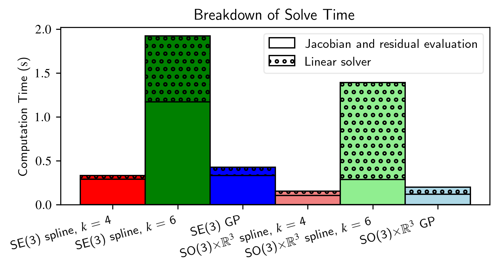
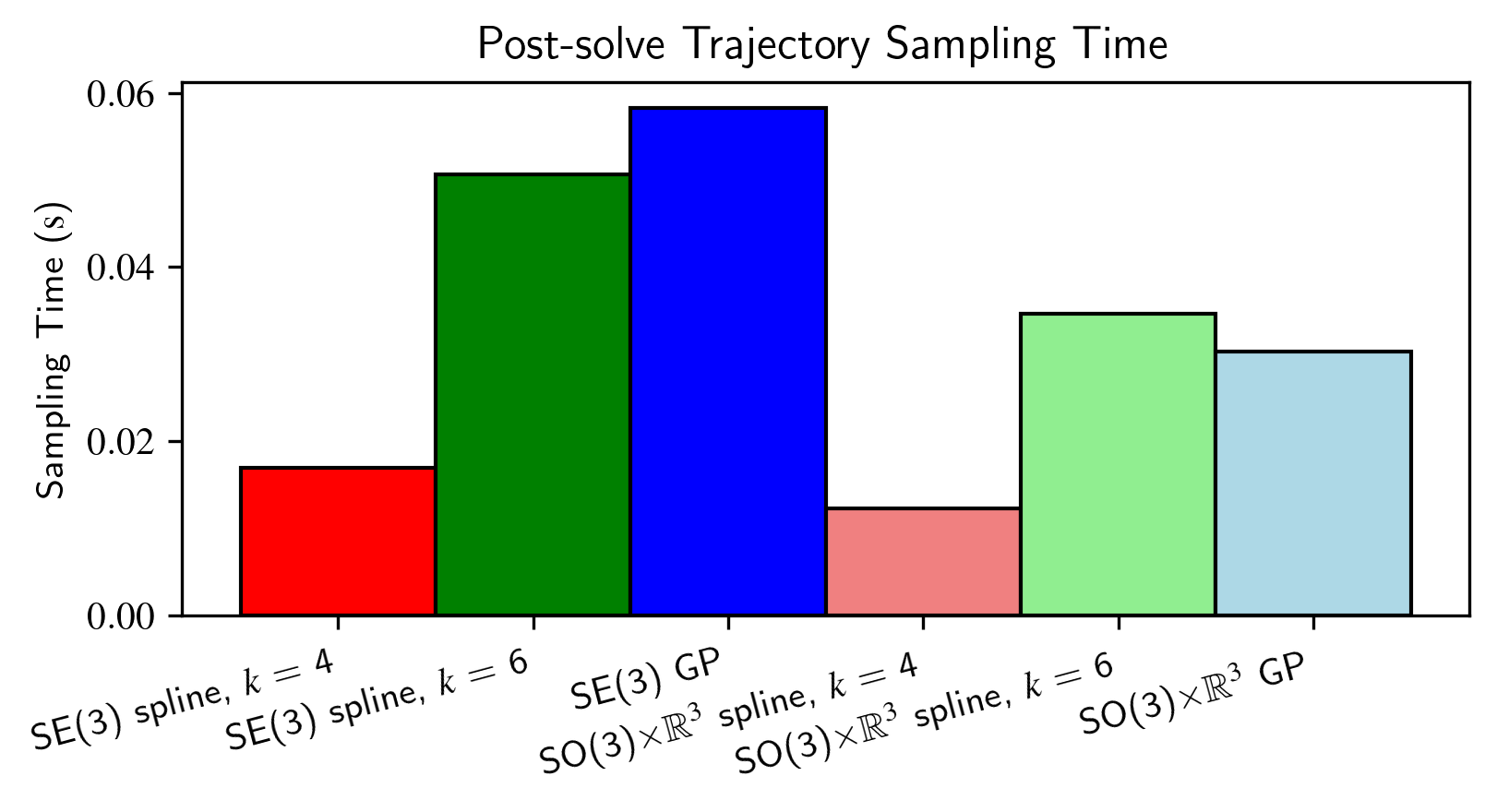
There were, however, significant differences in computation time between the methods. The GP-based methods required less computation time than the spline-based methods when not using IMU measurements. This is because the GP was only evaluated at the estimation times during optimization in this case, so no GP state interpolation (24) was required101010In this case, the problem is equivalent to discrete-time estimation.. When including IMU measurements, the solve times for GPs and splines with k=4𝑘4k=4 were comparable. However, splines with k=6𝑘6k=6 required significantly more solve time than the other methods, especially when using motion priors. Figure 12 gives a breakdown of the solve times for WNOJ trajectories when using both motion priors and IMU. The bottom part of the bars shows the amount of time spent evaluating residuals and their Jacobians, and the top part shows the amount of time spent solving the linear system of equations. For splines with k=6𝑘6k=6 most of the time is spent evaluating residuals and Jacobians, but there was also a large amount of time spent solving the linear system of equations. We elaborate more on these results in Section IX. Finally, Figure 13 shows the amount of time required to query the entire trajectory (pose and twist) at a rate of 1 kHzkHz\mathrm{k}\mathrm{H}\mathrm{z} after optimization. GPs on SE(3) required the most time, and splines with k=4𝑘4k=4 required the least.

Refer to caption
Figure 11: GP and spline trajectory error and solve time for the WNOJ trajectories.
Refer to caption
Figure 12: Solve time breakdown for the WNOJ trajectory results when using both motion priors and IMU.
Refer to caption
Figure 13: Total post-solve trajectory sampling times. Pose and twist were sampled uniformly along the 10 second trajectories at a rate of 1 kHzkHz\mathrm{k}\mathrm{H}\mathrm{z}.

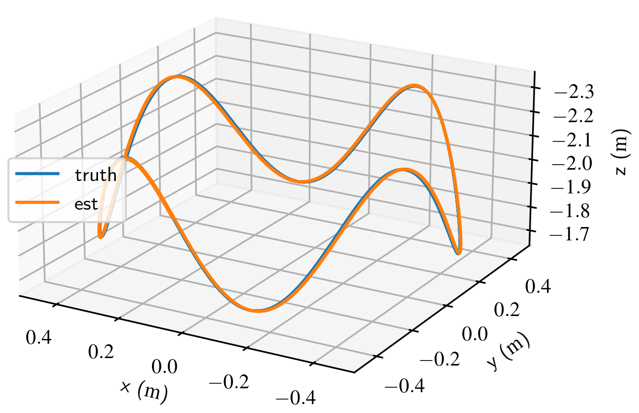
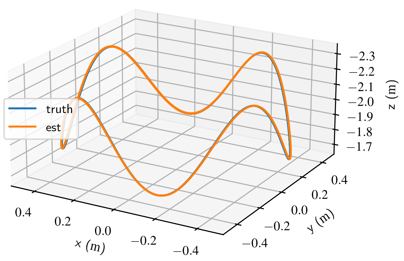
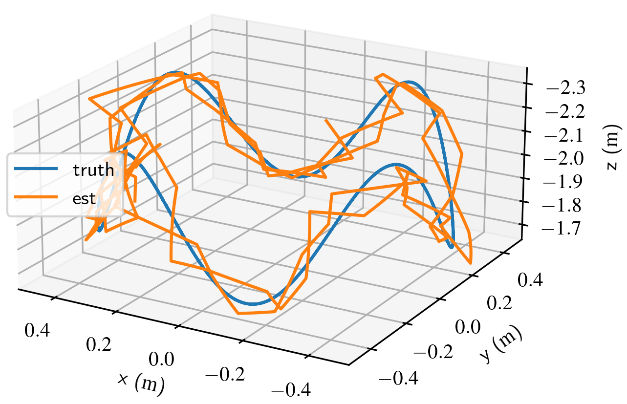
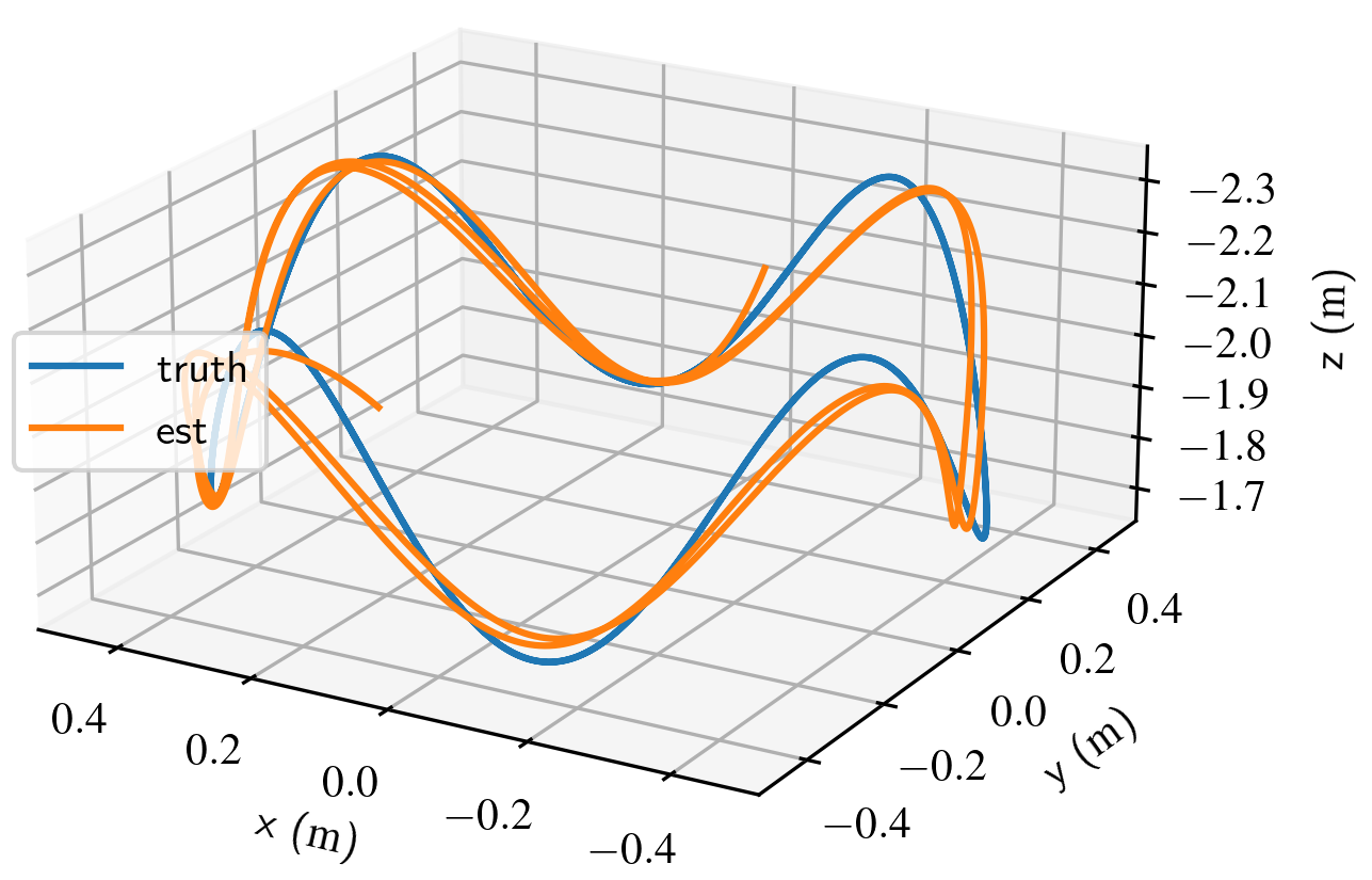
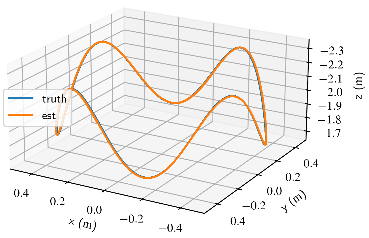
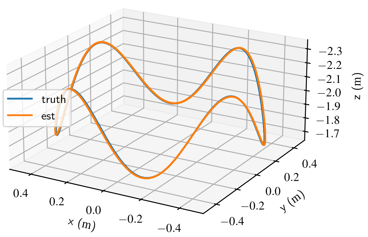
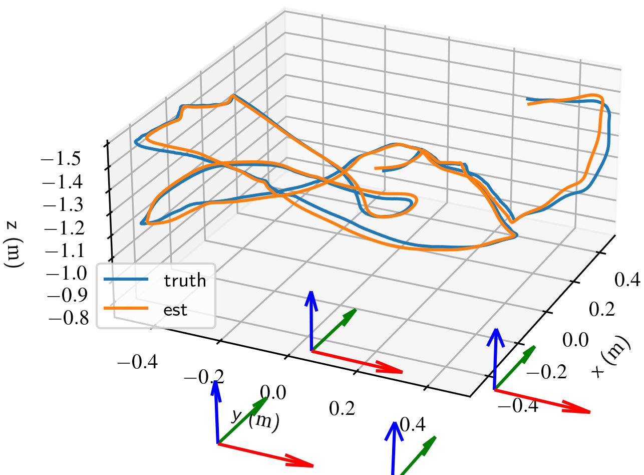
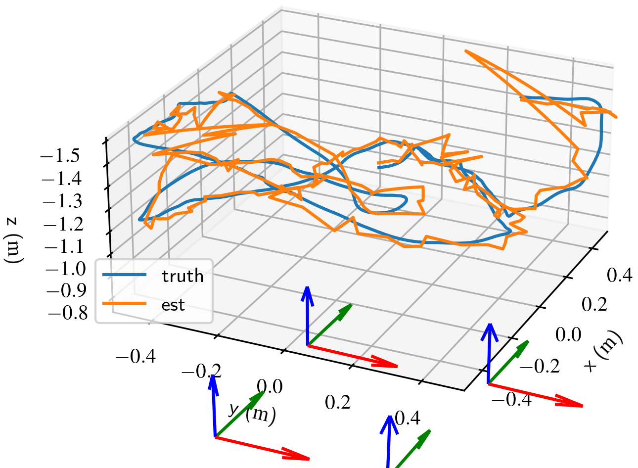
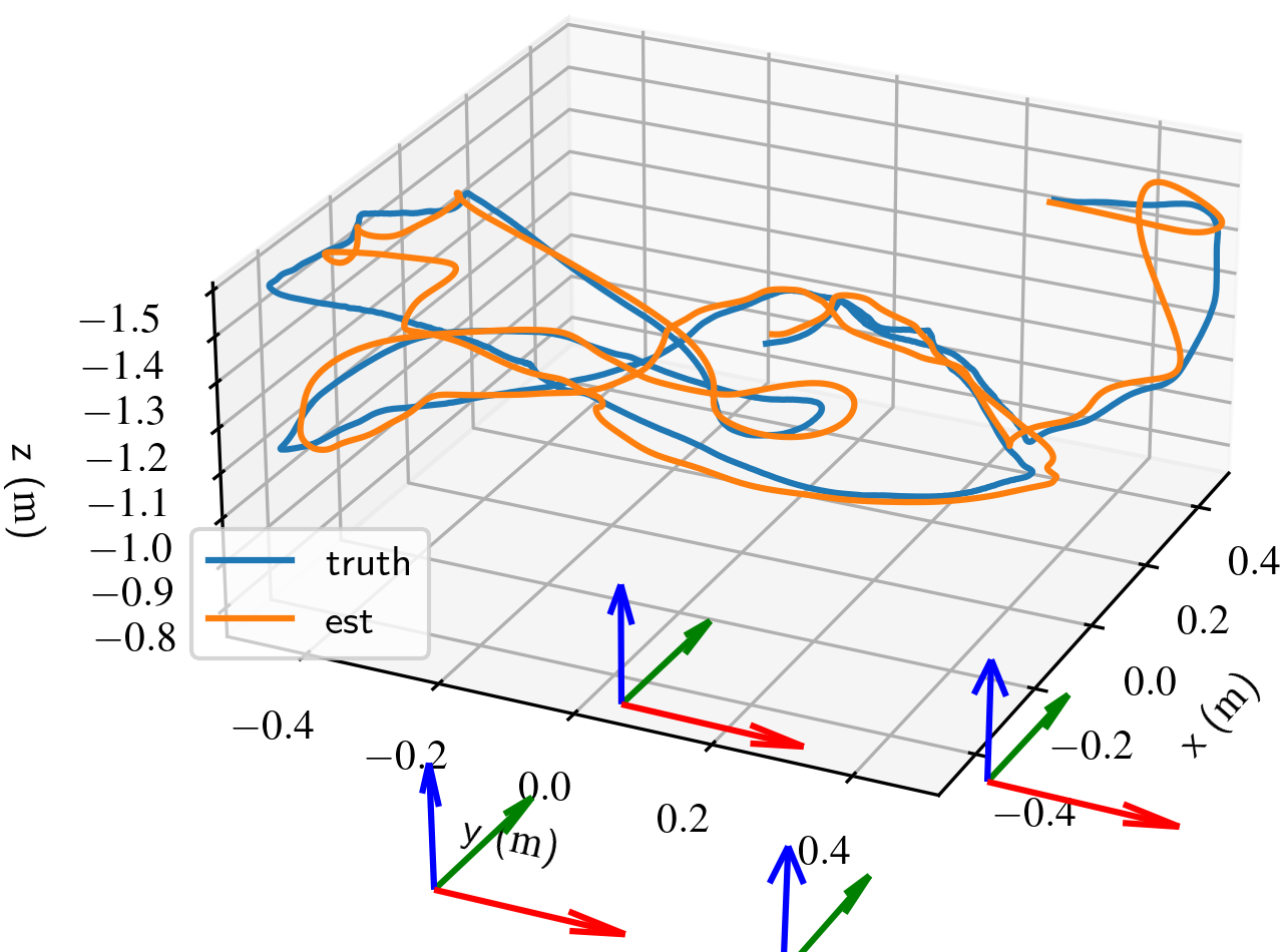
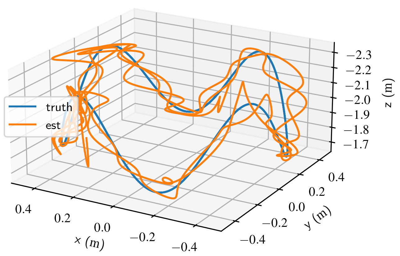
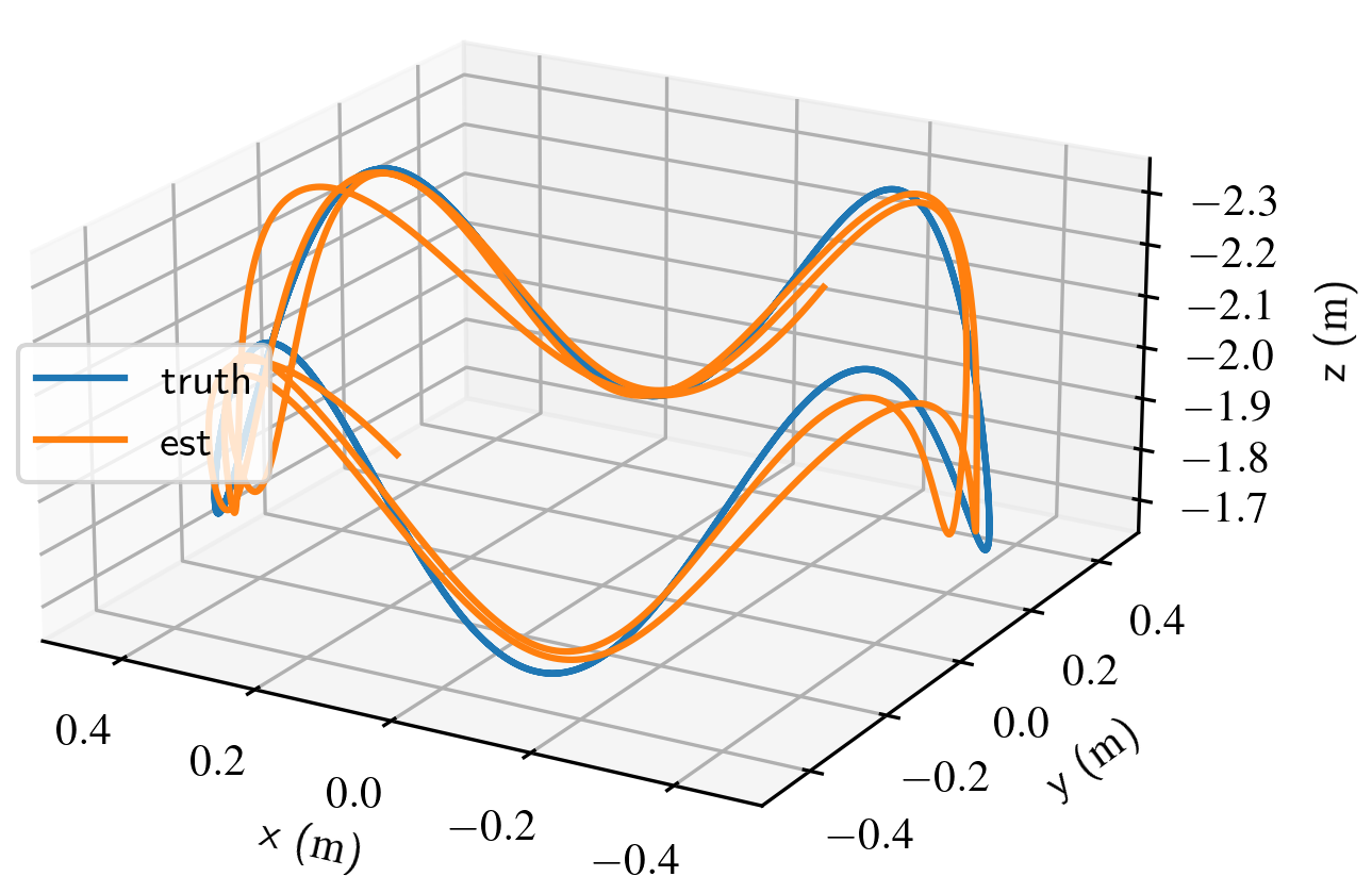
We additionally simulated a sinusoidal trajectory to compare each of these methods when the assumed motion model does not match the true motion of the system. The camera was moved along a circular trajectory such that the fiducial marker was always within the simulated FOV. In this scenario the variable fiducial pose covariance was used when simulating the camera measurements. Figures 14 and 15 show the resulting estimated trajectories with each type of regularization for a spline on SE(3) with k=4𝑘4k=4 and a GP on SE(3), respectively. It is evident that the motion priors have a profound impact on the smoothness of the estimate. However, the estimated trajectory is much more accurate when using IMU measurements. As we noted previously, using motion priors in addition to the IMU measurements does not seem to offer any improvement. It is interesting to note that, when using the same type of regularization, the spline and GP estimates appear to be very similar.
Refer to caption
(a) None
Refer to caption
(b) Motion priors
Refer to caption
(c) IMU
Refer to caption
(d) Motion priors + IMU
Figure 14: SE(3) spline (k=4𝑘4k=4) trajectory estimate for the sinusoidal trajectory with each type of regularization.
Refer to caption
(a) None
Refer to caption
(b) Motion priors
Refer to caption
(c) IMU
Refer to caption
(d) Motion priors + IMU
Figure 15: SE(3) GP trajectory estimate for the sinusoidal trajectory with each type of regularization.

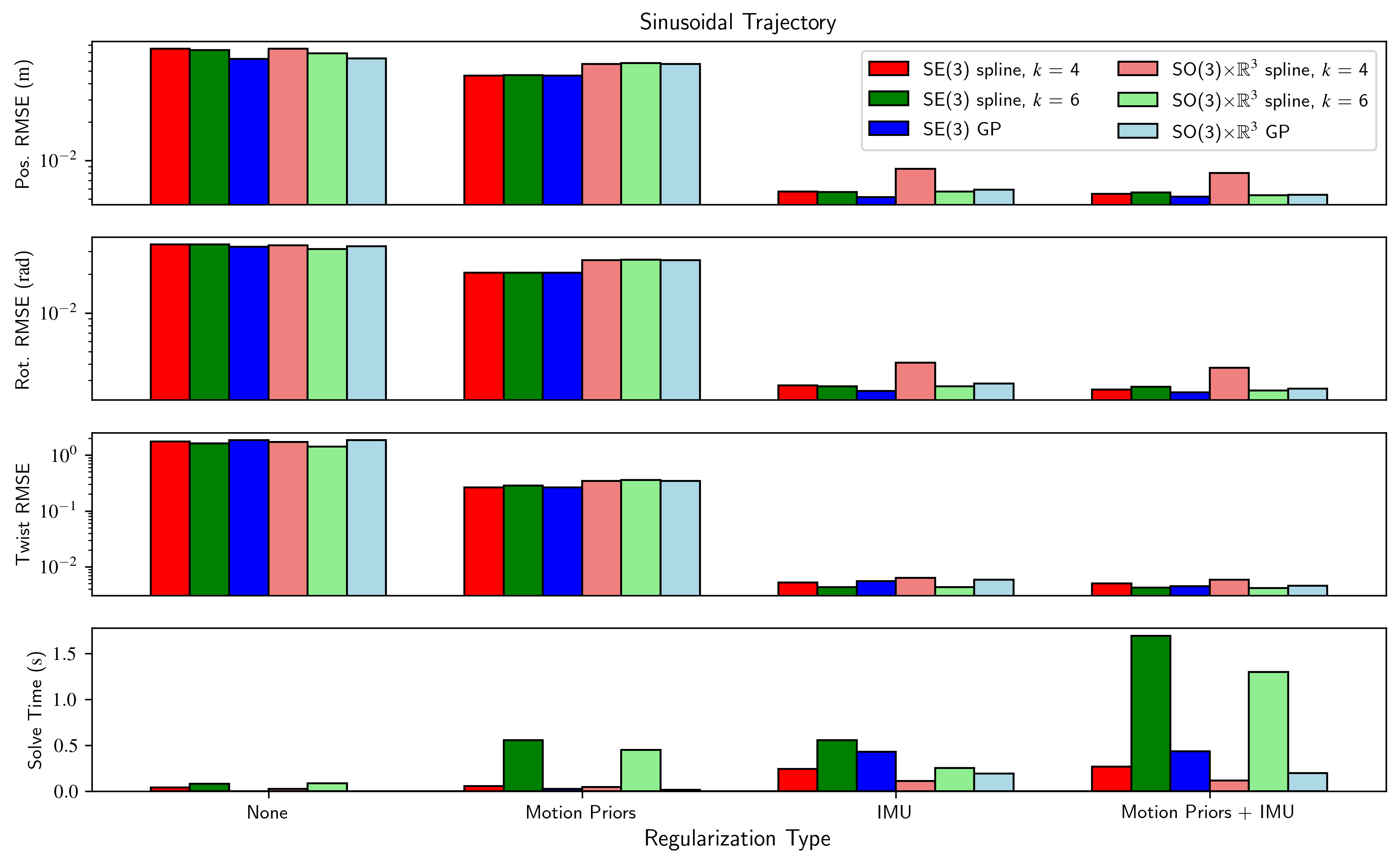
We ran 100 Monte Carlo trials for each estimation scenario on this sinusoidal trajectory. The results are shown in Figure 16. These results are similar and consistent with Figure 11. However, the motion priors did not have as significant an effect in lowering the position and rotation RMSE, likely because they did not match the true motion of the system. They did, however, cause a significant reduction in the twist RMSE because of their effect on the smoothness of the trajectory. Interestingly, the SO(3)×3absentsuperscript3\times\mathbb{R}^{3} trajectories often had lower accuracy than the SE(3) trajectories, especially for splines with k=4𝑘4k=4 when using IMU measurements.

Refer to caption
Figure 16: GP and spline trajectory error and solve time for the sinusoidal trajectory.

VIII IMU Hardware Comparison

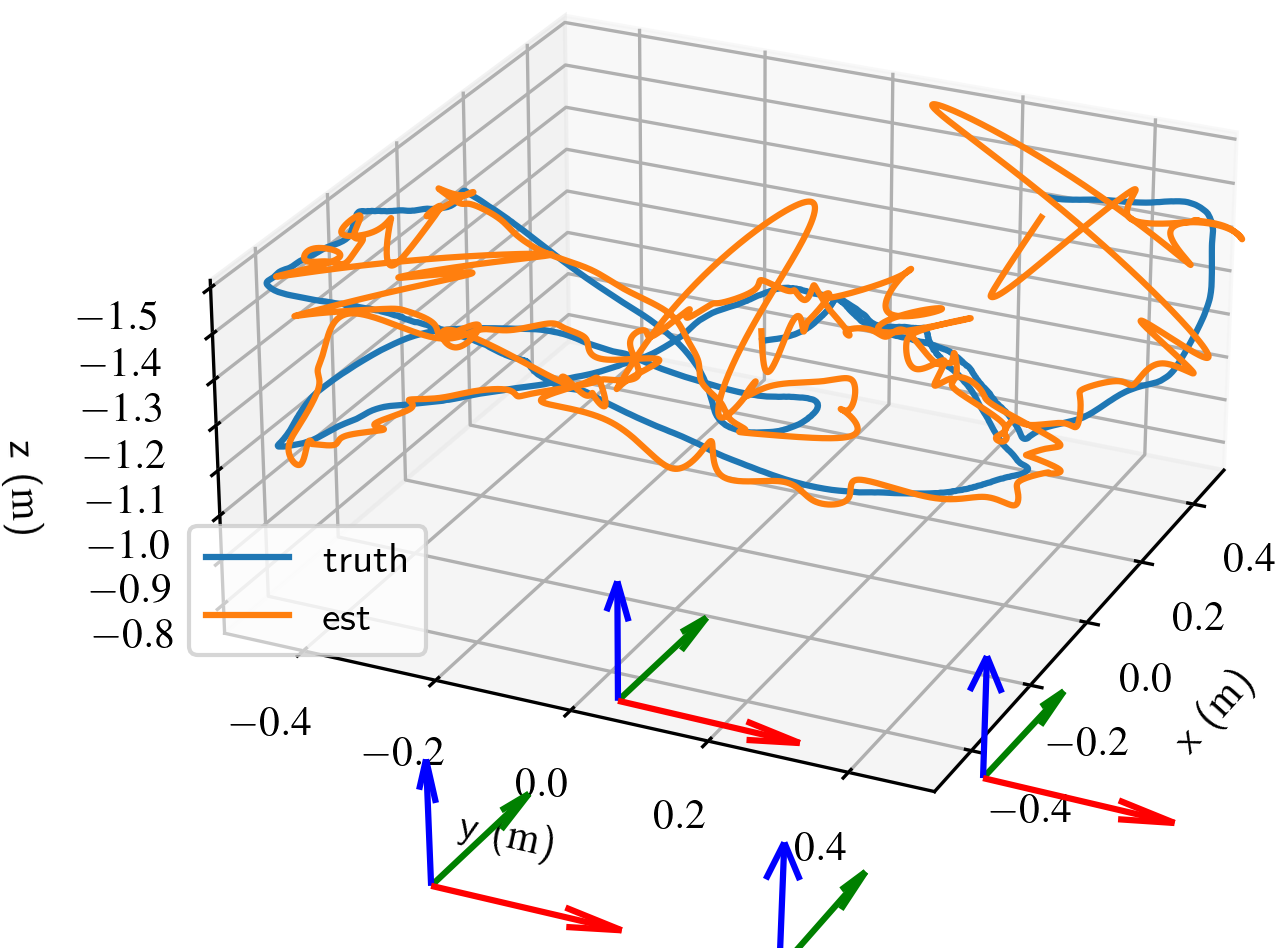
For our final comparison scenario, we again performed the experiment described in Section V-B, but used actual data from a camera and IMU rather than simulated data. We placed four AprilTag [46] fiducial markers in a room equipped with an Optitrack111111https://optitrack.com/ motion capture system that was used to obtain ground truth data. We maneuvered an Intel RealSense121212https://www.intelrealsense.com/ d435i camera/IMU in the environment while observing and detecting the fiducial markers. Relative pose measurements were collected at 10 HzHz\mathrm{H}\mathrm{z} and IMU measurements were collected at 100 HzHz\mathrm{H}\mathrm{z}. We gathered data from several trajectories and performed estimation using each of the methods described in Section VII (again with δt=0.1𝛿𝑡0.1\delta t=0.1 ss\mathrm{s} and nGP=1subscript𝑛GP1n_{\text{GP}}=1). After estimation, the relative transformation and time offset between the motion capture data and the estimated trajectory was optimized so that the ground truth and estimated trajectories could be directly compared. Figures 17 and 18 show resulting trajectories estimated using a spline on SE(3) (with k=4𝑘4k=4) and a GP on SE(3), respectively, using each type of regularization. Qualitatively, the results for the two methods are nearly identical when the same type of regularization is used. The motion priors had a profound impact on the smoothness of the trajectory, but the IMU enabled greater accuracy. Incorporating motion priors in addition to the IMU measurements appears to have had little to no effect.
Refer to caption
(a) None
Refer to caption
(b) Motion priors
Refer to caption
(c) IMU
Refer to caption
(d) Motion priors + IMU
Figure 17: SE(3) spline (k=4𝑘4k=4) trajectory estimate for a hardware trajectory with each type of regularization.
Refer to caption
(a) None
Refer to caption
(b) Motion priors
Refer to caption
(c) IMU
Refer to caption
(d) Motion priors + IMU
Figure 18: SE(3) GP trajectory estimate for a hardware trajectory with each type of regularization.

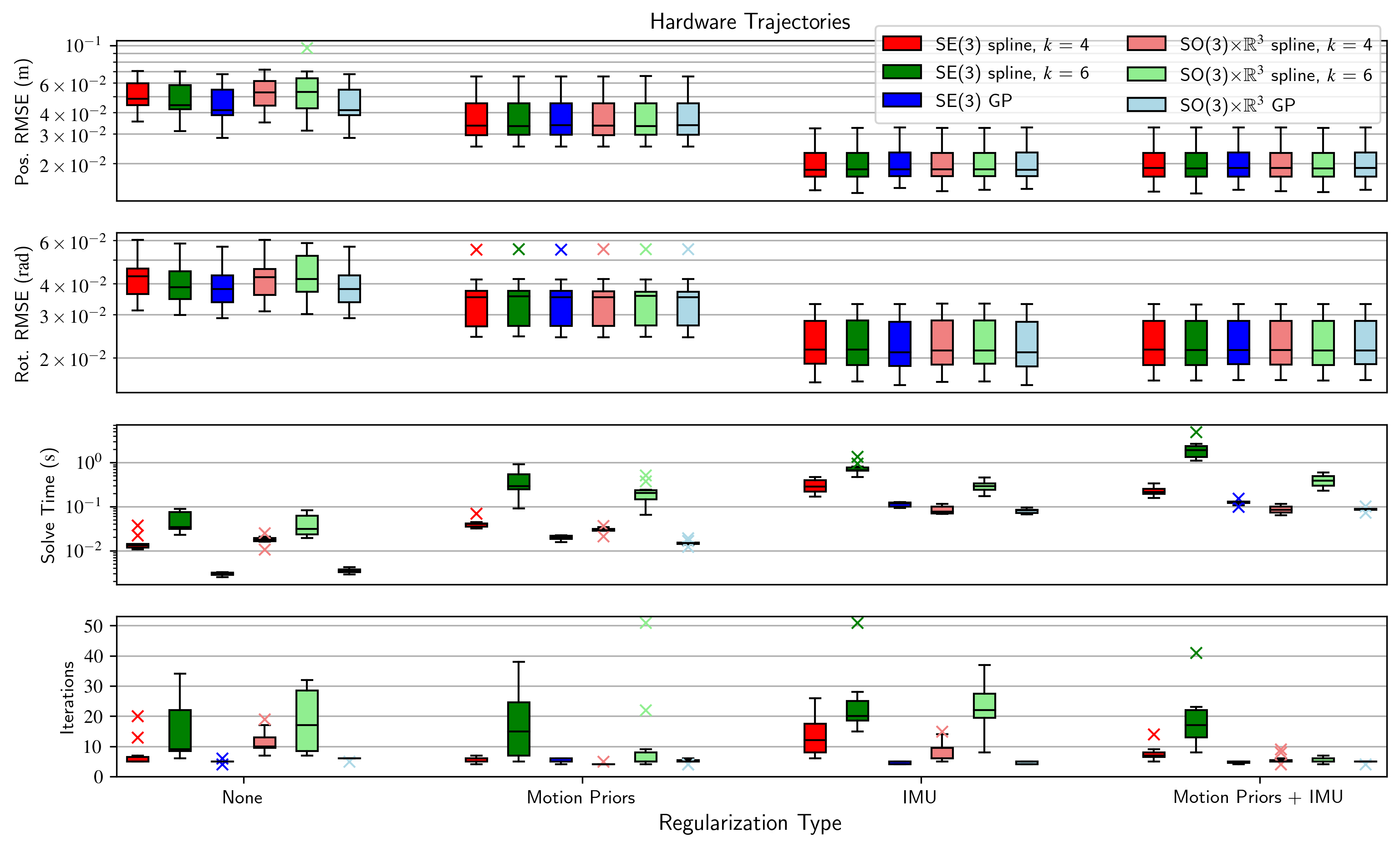
Figure 19 shows position and rotation RMSE131313The motion capture system did not provide ground truth velocity data, so the twist RMSE is not shown., solve time, and number of Levenburg-Marquardt iterations required to converge for each method using each type of regularization for eleven distinct 10 ss\mathrm{s} trajectories. These results follow a similar trend as Figures 11 and 16. Accuracy improved significantly when motion priors were incorporated, and even more so when IMU measurements were used, but including motion priors in addition to the IMU measurements did not offer improvement. All methods had similar trajectory accuracy when using the same regularization type (although the GP methods had slightly better accuracy than the spline methods when no regularization was used). There were significant differences in computation time and number of optimizer iterations between the methods. The methods performed on SO(3)×3SO3superscript3\text{SO}(3)\times\mathbb{R}^{3} had lower computation times than their SE(3) counterparts in all scenarios except when no regularization was used. GPs had faster solve times when IMU measurements were not used (again because no interpolation had to be done in these cases). However, when IMU measurements were used the solve times were mostly comparable between GPs and splines with k=4𝑘4k=4. The only exception to this is the case where motion priors were not used and estimation was done on SE(3), where splines with k=4𝑘4k=4 required a significantly higher number of iterations than GPs. Splines with k=6𝑘6k=6 had the highest solve times in all scenarios. They also required a large number of iterations to converge to a solution. It is interesting to note that using motion priors often allowed the spline-based methods to converge with fewer iterations (although overall solve time did not improve because of the inclusion of additional residual terms to evaluate). We will elaborate more on these results in Section IX.
Refer to caption
Figure 19: GP and spline trajectory error and solve time for the eleven hardware trajectories.

IX Discussion

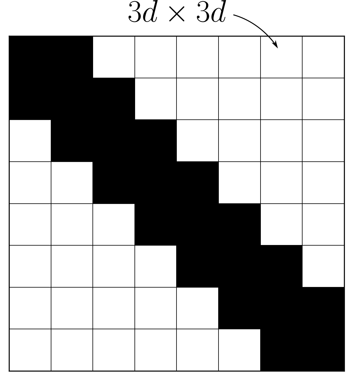
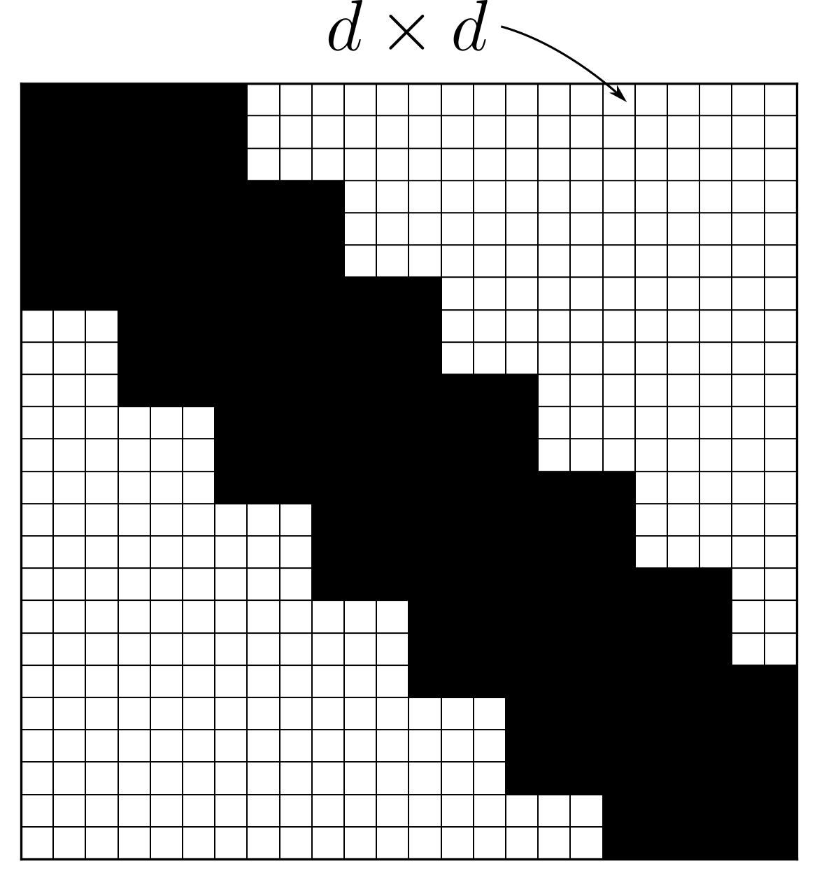
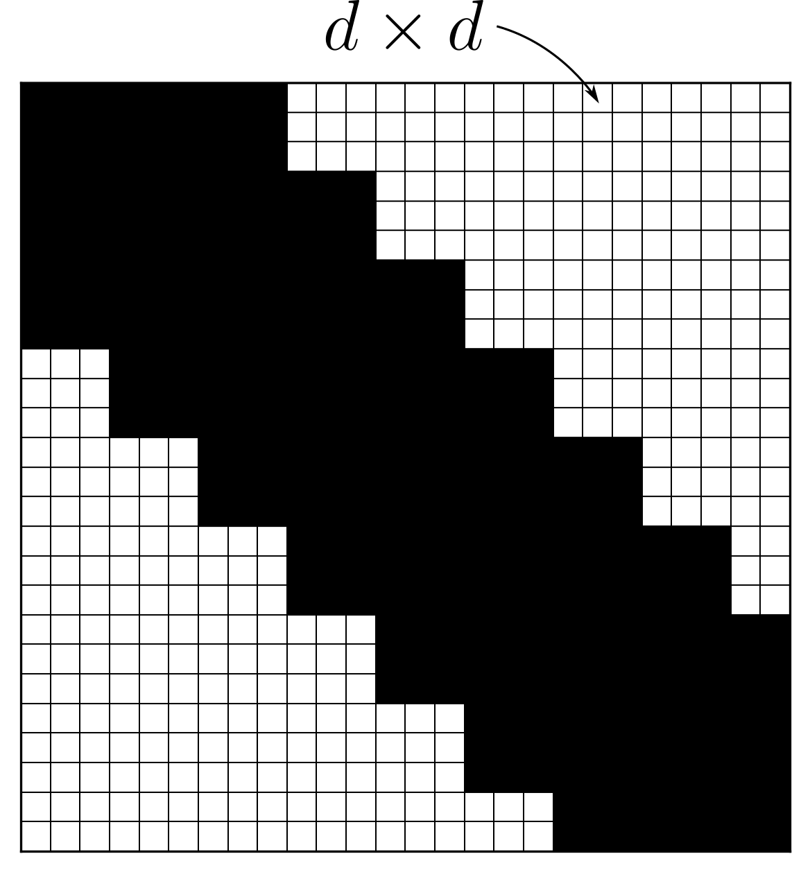
The overall purpose of this paper is to understand when one of the two continuous-time estimation methods is preferable to the other. However, the results of the comparisons in Sections VIVII, and VIII indicate that the two methods give similar results. When utilizing the same measurements and motion model, the resulting trajectory estimates are nearly identical. There are some significant differences in computation time, however. The most obvious is that splines with high order (e.g., k=6𝑘6k=6) take significantly longer to solve than GPs or splines with low order. The reason for this is straightforward. The state interpolation equation (32) for splines is dependent on k𝑘k control points, and Jacobian evaluation for each control point is O(k)𝑂𝑘O(k) (see Appendix -D). Thus the time complexity for evaluating each measurement residual is O(k2)𝑂superscript𝑘2O(k^{2}). In addition, the estimation problem becomes more dense with high spline orders. These factors are evident in Figure 12, where the Jacobian and residual evaluation time more than doubled and the linear solve time increased dramatically with k=6𝑘6k=6. Figure 20 shows the structure of the information matrix for splines with k=4𝑘4k=4 and k=6𝑘6k=6 (with δt/δt=1/3𝛿𝑡𝛿superscript𝑡13\delta t/\delta t^{\prime}=1/3), and GPs when using a WNOJ model. A large amount of fill-in occurs as the spline order increases. Conversely, the information matrix for GPs is always block-tridiagonal (although the individual blocks are three times the size of the spline estimation blocks because they each contain pose, velocity, and acceleration information).
Refer to caption
(a) Spline, k=4𝑘4k=4
Refer to caption
(b) Spline, k=6𝑘6k=6
Refer to caption
(c) GP
Figure 20: Example information matrix structures for spline estimation with orders 4 and 6 and for GP estimation, using a WNOJ model.

There is one benefit to choosing a higher spline order, however. The resulting spline has a higher degree-of-differentiability. Figure 21 shows the true and estimated accelerometer measurements from the simulated sinusoidal trajectory of Section VII for (from left to right) splines on SE(3) with k=4𝑘4k=4, k=6𝑘6k=6, and GPs on SE(3). Because splines with k=4𝑘4k=4 are twice continuously differentiable, the estimator essentially fits straight lines to the measurement data, whereas for k=6𝑘6k=6 it fits cubic polynomials. This factor did not significantly degrade the quality of the trajectory estimate in this case, so the higher order may not have been worth the additional computational cost. Figure 21 also shows a striking similarity between GP and spline (k=6𝑘6k=6) post-fit accelerometer residuals. This is because the acceleration component of the WNOJ GP interpolation equation (21) is cubic in τ𝜏\tau, so both splines with k=6𝑘6k=6 and GPs fit cubic polynomials to the accelerometer measurements. The main difference is that for GPs these polynomial segments are not continuously differentiable at the estimation times.

Refer to caption
Figure 21: Post-fit accelerometer data for (from left to right) splines with k=4𝑘4k=4, splines with k=6𝑘6k=6, and GPs on SE(3). Error is shown in green using the scale on the right.

There are a few additional points we would also like to bring to attention.

  • In almost all cases, decoupling the translation and rotation trajectories gave similar accuracy with less computation time. This is consistent with previous findings from [44, 47].

  • GPs required more time to query the trajectory after optimization than splines with k=4𝑘4k=4 did (see Figure 13). This may not be a significant factor when only the state at the most recent measurement time is needed (as is often the case in online estimation), because the time to query the trajectory once is several orders of magnitude lower than the optimization solve time. However, the difference between GPs and splines is significant enough to bring to attention. Note that despite the longer query times, GP trajectory solve times are comparable to splines with k=4𝑘4k=4 because they require fewer state interpolation Jacobians to evaluate per measurement time (2 versus 4).

  • The trajectory representation for GPs is directly motivated by the chosen motion model. This is not the case for splines. Our experiments show that this fact does not impact the trajectory quality. However, it does make GP interpolation seem more intuitive than spline interpolation.

  • In the case where the measurement times are all identical to the estimation times, GPs should be used instead of splines. This is evident from the solve times in Figure 19 when IMU measurements were not used. In these cases the GP interpolation function becomes identity for each measurement time and the problem is equivalent to a discrete-time estimation problem (while still allowing for interpolation after the solve).

  • The spline estimation parameters have a higher length of correlation in time than GPs. What we mean by this is that each control point will be correlated with the k1𝑘1k-1 control points immediately preceding and following it in the information matrix, whereas each GP parameter will only be correlated with the one parameter that precedes and follows it (see Figures 24, and 20). This higher amount of time correlation will become problematic, for example, in SLAM scenarios where a feature is viewed at multiple time instances during the estimation window 𝒲𝒲\mathcal{W} and is later marginalized. In this case, the spline information matrix will fill in more than the GP information matrix will. Our tests do not include such a scenario, but we acknowledge that this is a potential case where GPs may outperform splines in terms of computation time. More investigation is needed to verify this.

  • One potential benefit of using splines over GPs is that increasing the degree-of-differentiability is as simple as choosing a higher value of k𝑘k. For GPs, this requires using a more complicated motion model.

In summary, GPs and splines give comparable results if the same measurements and motion model are used, and if the chosen spline degree-of-differentiability matches the differentiability required by the motion model (e.g., k=3𝑘3k=3 for a WNOA model, k=4𝑘4k=4 for a WNOJ model). However, in the case that a high degree-of-differentiability is required, splines may be more convenient, and in the case that the measurement times match the estimation times (i.e., the problem can be solved with discrete-time estimation), GPs should be used.

X Conclusion

In this paper we presented a direct comparison between GP and spline-based continuous-time trajectory estimation. We introduced continuous-time estimation generally and showed how the same motion models used in [13, 27] can be generalized for use with both GPs and splines on vector spaces and Lie groups. We then compared the two methods with a simulated linear model and in a camera/IMU sensor fusion scenario. Our results indicate that the two methods achieve similar trajectory accuracy if the same motion model and measurements are used. Solve times are also similar so long as the spline order is chosen such that the degree-of-differentiability matches that of the GP. Choosing a higher spline order did not improve trajectory accuracy, while requiring significantly higher solve times.

-A GP Interpolation as Optimal Control

It is possible to arrive at the GP interpolation equation (19) using an optimal control perspective. Consider the linear system in (6), and suppose that the input 𝐮(t)𝐮𝑡\mathbf{u}(t) is known for all values of t𝑡t. The solution to the differential equation (6) is

𝐱(t)=𝚽(t,tn)𝐱n+At,tn[𝐮]+tnt𝚽(t,τ)𝐋𝐰(τ)𝑑τ𝐱𝑡𝚽𝑡subscript𝑡𝑛subscript𝐱𝑛subscript𝐴𝑡subscript𝑡𝑛delimited-[]𝐮superscriptsubscriptsubscript𝑡𝑛𝑡𝚽𝑡𝜏𝐋𝐰𝜏differential-d𝜏\mathbf{x}(t)=\boldsymbol{\Phi}(t,t_{n})\mathbf{x}_{n}+A_{t,t_{n}}[\mathbf{u}]+\int_{t_{n}}^{t}\boldsymbol{\Phi}(t,\tau)\mathbf{L}\mathbf{w}(\tau)d\tau (44)

where t[tn,tn+1]𝑡subscript𝑡𝑛subscript𝑡𝑛1t\in[t_{n},t_{n+1}], 𝐱l=𝐱(tl)subscript𝐱𝑙𝐱subscript𝑡𝑙\mathbf{x}_{l}=\mathbf{x}(t_{l}), and

Aτ,τ[𝐮]=ττ𝚽(s,τ)𝐁𝐮(s)𝑑s.subscript𝐴𝜏superscript𝜏delimited-[]𝐮superscriptsubscriptsuperscript𝜏𝜏𝚽𝑠superscript𝜏𝐁𝐮𝑠differential-d𝑠A_{\tau,\tau^{\prime}}[\mathbf{u}]=\int_{\tau^{\prime}}^{\tau}\boldsymbol{\Phi}(s,\tau^{\prime})\mathbf{B}\mathbf{u}(s)ds. (45)

Our goal is to find the noise trajectory 𝐰(t)𝐰𝑡\mathbf{w}(t) that satisfies

min𝐰(t)tntn+1𝐰(τ)𝑑τs.t.𝐱˙=𝐀𝐱+𝐁𝐮+𝐋𝐰𝐱n=𝐱¯n𝐱n+1=𝐱¯n+1.subscript𝐰𝑡superscriptsubscriptsubscript𝑡𝑛subscript𝑡𝑛1delimited-∥∥𝐰𝜏differential-d𝜏s.t.˙𝐱absent𝐀𝐱𝐁𝐮𝐋𝐰subscript𝐱𝑛absentsubscript¯𝐱𝑛subscript𝐱𝑛1absentsubscript¯𝐱𝑛1\begin{gathered}\min_{\mathbf{w}(t)}\quad\int_{t_{n}}^{t_{n+1}}\lVert\mathbf{w}(\tau)\rVert d\tau\\ \begin{aligned} \text{s.t.}\qquad\dot{\mathbf{x}}&=\mathbf{A}\mathbf{x}+\mathbf{B}\mathbf{u}+\mathbf{L}\mathbf{w}\\ \mathbf{x}_{n}&=\bar{\mathbf{x}}_{n}\\ \mathbf{x}_{n+1}&=\bar{\mathbf{x}}_{n+1}.\end{aligned}\end{gathered} (46)

Define the reachability Gramian

WR(t,tn)=tnt𝚽(t,τ)𝐋𝐋𝚽(t,τ)𝑑τsubscript𝑊𝑅𝑡subscript𝑡𝑛superscriptsubscriptsubscript𝑡𝑛𝑡𝚽𝑡𝜏superscript𝐋𝐋top𝚽superscript𝑡𝜏topdifferential-d𝜏W_{R}(t,t_{n})=\int_{t_{n}}^{t}\boldsymbol{\Phi}(t,\tau)\mathbf{L}\mathbf{L}^{\top}\boldsymbol{\Phi}(t,\tau)^{\top}d\tau (47)

and note that WR(t,tn)=𝐐1𝐐tsubscript𝑊𝑅𝑡subscript𝑡𝑛superscript𝐐1subscript𝐐𝑡W_{R}(t,t_{n})=\mathbf{Q}^{-1}\mathbf{Q}_{t}, where 𝐐𝐐\mathbf{Q} is treated as a matrix that multiplies block-wise into 𝐐tsubscript𝐐𝑡\mathbf{Q}_{t}. If we assume that the system (𝐀,𝐋)𝐀𝐋(\mathbf{A},\mathbf{L}) is controllable, then the reachability Gramian is invertible. It is a well-known result that the solution to (46) is [48]

𝐰(t)=𝐋𝚽(tn+1,t)𝝁n+1,superscript𝐰𝑡superscript𝐋top𝚽superscriptsubscript𝑡𝑛1𝑡topsubscript𝝁𝑛1\mathbf{w}^{\ast}(t)=\mathbf{L}^{\top}\boldsymbol{\Phi}(t_{n+1},t)^{\top}\boldsymbol{\mu}_{n+1}, (48)

where

𝝁n+1=WR(tn+1,tn)1(𝐱n+1𝚽(tn+1,tn)𝐱nAtn+1,tn[𝐮]).subscript𝝁𝑛1subscript𝑊𝑅superscriptsubscript𝑡𝑛1subscript𝑡𝑛1subscript𝐱𝑛1𝚽subscript𝑡𝑛1subscript𝑡𝑛subscript𝐱𝑛subscript𝐴subscript𝑡𝑛1subscript𝑡𝑛delimited-[]𝐮\begin{gathered}\boldsymbol{\mu}_{n+1}=W_{R}(t_{n+1},t_{n})^{-1}\left(\mathbf{x}_{n+1}-\boldsymbol{\Phi}(t_{n+1},t_{n})\mathbf{x}_{n}\right.\\ \left.\qquad\qquad\qquad\qquad-\>A_{t_{n+1},t_{n}}[\mathbf{u}]\right).\end{gathered} (49)

We can plug this noise input into (44) to find the interpolated state:

𝐱(t)=𝚽(t,tn)𝐱n+At,tn[𝐮]+tnt𝚽(t,τ)𝐋𝐰(τ)𝑑τ=𝚽(t,tn)𝐱n+At,tn[𝐮]+𝐐(tnt𝚽(t,τ)𝐋𝐋𝚽(tn+1,τ)dτ)𝐐tn+11(𝐱n+1𝚽(tn+1,tn)𝐱nAtn+1,tn[𝐮])=𝚽(t,tn)𝐱n+At,tn[𝐮]+𝐐(tnt𝚽(t,τ)𝐋𝐋𝚽(t,τ)dτ)𝚽(tn+1,t)𝐐tn+11(𝐱n+1𝚽(tn+1,tn)𝐱nAtn+1,tn[𝐮])=𝚽(t,tn)𝐱n+At,tn[𝐮]+𝐐t𝚽(tn+1,t)𝐐tn+11(𝐱n+1𝚽(tn+1,tn)𝐱nAtn+1,tn[𝐮])=𝚲(t)𝐱n+𝛀(t)(𝐱n+1Atn+1,tn[𝐮])+At,tn[𝐮].𝐱𝑡𝚽𝑡subscript𝑡𝑛subscript𝐱𝑛subscript𝐴𝑡subscript𝑡𝑛delimited-[]𝐮superscriptsubscriptsubscript𝑡𝑛𝑡𝚽𝑡𝜏superscript𝐋𝐰𝜏differential-d𝜏𝚽𝑡subscript𝑡𝑛subscript𝐱𝑛subscript𝐴𝑡subscript𝑡𝑛delimited-[]𝐮𝐐superscriptsubscriptsubscript𝑡𝑛𝑡𝚽𝑡𝜏superscript𝐋𝐋top𝚽superscriptsubscript𝑡𝑛1𝜏top𝑑𝜏superscriptsubscript𝐐subscript𝑡𝑛11subscript𝐱𝑛1𝚽subscript𝑡𝑛1subscript𝑡𝑛subscript𝐱𝑛subscript𝐴subscript𝑡𝑛1subscript𝑡𝑛delimited-[]𝐮𝚽𝑡subscript𝑡𝑛subscript𝐱𝑛subscript𝐴𝑡subscript𝑡𝑛delimited-[]𝐮𝐐superscriptsubscriptsubscript𝑡𝑛𝑡𝚽𝑡𝜏superscript𝐋𝐋top𝚽superscript𝑡𝜏top𝑑𝜏𝚽superscriptsubscript𝑡𝑛1𝑡topsuperscriptsubscript𝐐subscript𝑡𝑛11subscript𝐱𝑛1𝚽subscript𝑡𝑛1subscript𝑡𝑛subscript𝐱𝑛subscript𝐴subscript𝑡𝑛1subscript𝑡𝑛delimited-[]𝐮𝚽𝑡subscript𝑡𝑛subscript𝐱𝑛subscript𝐴𝑡subscript𝑡𝑛delimited-[]𝐮subscript𝐐𝑡𝚽superscriptsubscript𝑡𝑛1𝑡topsuperscriptsubscript𝐐subscript𝑡𝑛11subscript𝐱𝑛1𝚽subscript𝑡𝑛1subscript𝑡𝑛subscript𝐱𝑛subscript𝐴subscript𝑡𝑛1subscript𝑡𝑛delimited-[]𝐮𝚲𝑡subscript𝐱𝑛𝛀𝑡subscript𝐱𝑛1subscript𝐴subscript𝑡𝑛1subscript𝑡𝑛delimited-[]𝐮subscript𝐴𝑡subscript𝑡𝑛delimited-[]𝐮\begin{split}\mathbf{x}(t)&=\boldsymbol{\Phi}(t,t_{n})\mathbf{x}_{n}+A_{t,t_{n}}[\mathbf{u}]+\int_{t_{n}}^{t}\boldsymbol{\Phi}(t,\tau)\mathbf{L}\mathbf{w}^{\ast}(\tau)d\tau\\ &=\boldsymbol{\Phi}(t,t_{n})\mathbf{x}_{n}+A_{t,t_{n}}[\mathbf{u}]\\ &\quad+\mathbf{Q}\left(\int_{t_{n}}^{t}\boldsymbol{\Phi}(t,\tau)\mathbf{L}\mathbf{L}^{\top}\boldsymbol{\Phi}(t_{n+1},\tau)^{\top}d\tau\right)\cdot\\ &\qquad\mathbf{Q}_{t_{n+1}}^{-1}\left(\mathbf{x}_{n+1}-\boldsymbol{\Phi}(t_{n+1},t_{n})\mathbf{x}_{n}-A_{t_{n+1},t_{n}}[\mathbf{u}]\right)\\ &=\boldsymbol{\Phi}(t,t_{n})\mathbf{x}_{n}+A_{t,t_{n}}[\mathbf{u}]\\ &\quad+\mathbf{Q}\left(\int_{t_{n}}^{t}\boldsymbol{\Phi}(t,\tau)\mathbf{L}\mathbf{L}^{\top}\boldsymbol{\Phi}(t,\tau)^{\top}d\tau\right)\boldsymbol{\Phi}(t_{n+1},t)^{\top}\cdot\\ &\qquad\mathbf{Q}_{t_{n+1}}^{-1}\left(\mathbf{x}_{n+1}-\boldsymbol{\Phi}(t_{n+1},t_{n})\mathbf{x}_{n}-A_{t_{n+1},t_{n}}[\mathbf{u}]\right)\\ &=\boldsymbol{\Phi}(t,t_{n})\mathbf{x}_{n}+A_{t,t_{n}}[\mathbf{u}]\\ &\quad+\mathbf{Q}_{t}\boldsymbol{\Phi}(t_{n+1},t)^{\top}\mathbf{Q}_{t_{n+1}}^{-1}\cdot\\ &\qquad\left(\mathbf{x}_{n+1}-\boldsymbol{\Phi}(t_{n+1},t_{n})\mathbf{x}_{n}-A_{t_{n+1},t_{n}}[\mathbf{u}]\right)\\ &=\boldsymbol{\Lambda}(t)\mathbf{x}_{n}+\boldsymbol{\Omega}(t)(\mathbf{x}_{n+1}-A_{t_{n+1},t_{n}}[\mathbf{u}])+A_{t,t_{n}}[\mathbf{u}].\end{split} (50)

Noting that the prior terms in (19) are

𝐱ˇ(τ)=𝚽(τ,tn)𝐱ˇn+Aτ,tn[𝐮],ˇ𝐱𝜏𝚽𝜏subscript𝑡𝑛subscriptˇ𝐱𝑛subscript𝐴𝜏subscript𝑡𝑛delimited-[]𝐮\check{\mathbf{x}}(\tau)=\boldsymbol{\Phi}(\tau,t_{n})\check{\mathbf{x}}_{n}+A_{\tau,t_{n}}[\mathbf{u}], (51)

it can be seen that (50) and (19) are equivalent when 𝐱n=𝐱¯n,𝐱n+1=𝐱¯n+1formulae-sequencesubscript𝐱𝑛subscript¯𝐱𝑛subscript𝐱𝑛1subscript¯𝐱𝑛1\mathbf{x}_{n}=\bar{\mathbf{x}}_{n},\ \mathbf{x}_{n+1}=\bar{\mathbf{x}}_{n+1}, which must be the case due to the constraints in (46).

-B Lie Group Gaussian Process Derivatives

Here we derive the time derivatives of (22).

ddt(𝝃n(t))=limh0Log(g(t+h)g¯n1)𝝃n(t)h=limh0Log(Exp(g˙(t)h)g(t)g¯n1)𝝃n(t)h=Jl1(𝝃n(t))g˙(t).𝑑𝑑𝑡subscript𝝃𝑛𝑡subscript0Log𝑔𝑡superscriptsubscript¯𝑔𝑛1subscript𝝃𝑛𝑡subscript0LogExp˙𝑔𝑡𝑔𝑡superscriptsubscript¯𝑔𝑛1subscript𝝃𝑛𝑡superscriptsubscript𝐽𝑙1subscript𝝃𝑛𝑡˙𝑔𝑡\begin{split}\frac{d}{dt}(\boldsymbol{\xi}_{n}(t))&=\lim_{h\to 0}\frac{\text{Log}(g(t+h)\bar{g}_{n}^{-1})-\boldsymbol{\xi}_{n}(t)}{h}\\ &=\lim_{h\to 0}\frac{\text{Log}(\text{Exp}(\dot{g}(t)h)g(t)\bar{g}_{n}^{-1})-\boldsymbol{\xi}_{n}(t)}{h}\\ &=J_{l}^{-1}(\boldsymbol{\xi}_{n}(t))\dot{g}(t).\end{split} (52)

To compute the second derivative, we use the chain rule

ddt(𝝃˙n(t))=Jl1(𝝃n(t))g¨(t)+ddt(Jl1(𝝃n(t)))g˙(t).𝑑𝑑𝑡subscript˙𝝃𝑛𝑡superscriptsubscript𝐽𝑙1subscript𝝃𝑛𝑡¨𝑔𝑡𝑑𝑑𝑡superscriptsubscript𝐽𝑙1subscript𝝃𝑛𝑡˙𝑔𝑡\frac{d}{dt}(\dot{\boldsymbol{\xi}}_{n}(t))=J_{l}^{-1}(\boldsymbol{\xi}_{n}(t))\ddot{g}(t)+\frac{d}{dt}\left(J_{l}^{-1}(\boldsymbol{\xi}_{n}(t))\right)\dot{g}(t). (53)

We know of no simple way to compute ddt(Jl1(𝝃n(t)))𝑑𝑑𝑡superscriptsubscript𝐽𝑙1subscript𝝃𝑛𝑡\frac{d}{dt}\left(J_{l}^{-1}(\boldsymbol{\xi}_{n}(t))\right). Rather, we approximate it using a first-order Taylor series expansion,

ddt(Jl1(𝝃n(t)))ddt(𝐈12𝝃n(t))=12𝝃˙n(t).𝑑𝑑𝑡superscriptsubscript𝐽𝑙1subscript𝝃𝑛𝑡𝑑𝑑𝑡𝐈12subscript𝝃𝑛superscript𝑡12subscript˙𝝃𝑛superscript𝑡\frac{d}{dt}\left(J_{l}^{-1}(\boldsymbol{\xi}_{n}(t))\right)\approx\frac{d}{dt}\left(\mathbf{I}-\frac{1}{2}\boldsymbol{\xi}_{n}(t)^{\curlywedge}\right)=-\frac{1}{2}\dot{\boldsymbol{\xi}}_{n}(t)^{\curlywedge}. (54)

This approximation is reasonable so long as 𝝃˙n(t)subscript˙𝝃𝑛𝑡\dot{\boldsymbol{\xi}}_{n}(t) remains small throughout the interval [tn,tn+1]subscript𝑡𝑛subscript𝑡𝑛1[t_{n},t_{n+1}]. Applying this approximation, we arrive at (15).

-C Lie Group Gaussian Process Jacobians

-C1 Global Variable Jacobians

We need the Jacobians of the interpolated global variables 𝐱(t)𝐱𝑡\mathbf{x}(t) in (24) with respect to the estimation states 𝐱¯n,𝐱¯n+1subscript¯𝐱𝑛subscript¯𝐱𝑛1\bar{\mathbf{x}}_{n},\bar{\mathbf{x}}_{n+1}, where tnttn+1subscript𝑡𝑛𝑡subscript𝑡𝑛1t_{n}\leq t\leq t_{n+1}. We will start with g(t)𝑔𝑡g(t). Note that

g(t)g¯n=g(t)g¯n+g(t)𝝃n(t)𝝃n(t)g¯n,g(t)g¯n+1=g(t)𝝃n(t)𝝃n(t)g¯n+1,g(t)g¯˙n=g(t)𝝃n(t)𝝃n(t)g¯˙n,g(t)g¯˙n+1=g(t)𝝃n(t)𝝃n(t)g¯˙n+1,g(t)g¯¨n=g(t)𝝃n(t)𝝃n(t)g¯¨n,g(t)g¯¨n+1=g(t)𝝃n(t)𝝃i(t)g¯¨n+1.formulae-sequence𝑔𝑡subscript¯𝑔𝑛𝑔𝑡subscript¯𝑔𝑛𝑔𝑡subscript𝝃𝑛𝑡subscript𝝃𝑛𝑡subscript¯𝑔𝑛formulae-sequence𝑔𝑡subscript¯𝑔𝑛1𝑔𝑡subscript𝝃𝑛𝑡subscript𝝃𝑛𝑡subscript¯𝑔𝑛1formulae-sequence𝑔𝑡subscript˙¯𝑔𝑛𝑔𝑡subscript𝝃𝑛𝑡subscript𝝃𝑛𝑡subscript˙¯𝑔𝑛formulae-sequence𝑔𝑡subscript˙¯𝑔𝑛1𝑔𝑡subscript𝝃𝑛𝑡subscript𝝃𝑛𝑡subscript˙¯𝑔𝑛1formulae-sequence𝑔𝑡subscript¨¯𝑔𝑛𝑔𝑡subscript𝝃𝑛𝑡subscript𝝃𝑛𝑡subscript¨¯𝑔𝑛𝑔𝑡subscript¨¯𝑔𝑛1𝑔𝑡subscript𝝃𝑛𝑡subscript𝝃𝑖𝑡subscript¨¯𝑔𝑛1\begin{gathered}\frac{\partial g(t)}{\partial\bar{g}_{n}}=\frac{\partial g(t)}{\partial\bar{g}_{n}}+\frac{\partial g(t)}{\partial\boldsymbol{\xi}_{n}(t)}\frac{\partial\boldsymbol{\xi}_{n}(t)}{\partial\bar{g}_{n}},\\ \frac{\partial g(t)}{\partial\bar{g}_{n+1}}=\frac{\partial g(t)}{\partial\boldsymbol{\xi}_{n}(t)}\frac{\partial\boldsymbol{\xi}_{n}(t)}{\partial\bar{g}_{n+1}},\\ \frac{\partial g(t)}{\partial\dot{\bar{g}}_{n}}=\frac{\partial g(t)}{\partial\boldsymbol{\xi}_{n}(t)}\frac{\partial\boldsymbol{\xi}_{n}(t)}{\partial\dot{\bar{g}}_{n}},\\ \frac{\partial g(t)}{\partial\dot{\bar{g}}_{n+1}}=\frac{\partial g(t)}{\partial\boldsymbol{\xi}_{n}(t)}\frac{\partial\boldsymbol{\xi}_{n}(t)}{\partial\dot{\bar{g}}_{n+1}},\\ \frac{\partial g(t)}{\partial\ddot{\bar{g}}_{n}}=\frac{\partial g(t)}{\partial\boldsymbol{\xi}_{n}(t)}\frac{\partial\boldsymbol{\xi}_{n}(t)}{\partial\ddot{\bar{g}}_{n}},\\ \frac{\partial g(t)}{\partial\ddot{\bar{g}}_{n+1}}=\frac{\partial g(t)}{\partial\boldsymbol{\xi}_{n}(t)}\frac{\partial\boldsymbol{\xi}_{i}(t)}{\partial\ddot{\bar{g}}_{n+1}}.\end{gathered} (55)

These are computed as

gg¯n=lim𝝉𝟎Log(Exp(𝝃n)Exp(𝝉)g¯n(Exp(𝝃n)g¯n)1)𝝉=AdExp(𝝃n),g𝝃n=lim𝝉𝟎Log(Exp(𝝃n+𝝉)g¯n(Exp(𝝃n)g¯n)1)τ=lim𝝉𝟎Log(Exp(Jl(𝝃n)𝝉)Exp(𝝃n)Exp(𝝃n)1)𝝉=Jl(𝝃n).formulae-sequence𝑔subscript¯𝑔𝑛subscript𝝉0LogExpsubscript𝝃𝑛Exp𝝉subscript¯𝑔𝑛superscriptExpsubscript𝝃𝑛subscript¯𝑔𝑛1𝝉subscriptAdExpsubscript𝝃𝑛𝑔subscript𝝃𝑛subscript𝝉0LogExpsubscript𝝃𝑛𝝉subscript¯𝑔𝑛superscriptExpsubscript𝝃𝑛subscript¯𝑔𝑛1𝜏subscriptbold-→𝝉0LogExpsubscript𝐽𝑙subscript𝝃𝑛𝝉Expsubscript𝝃𝑛Expsuperscriptsubscript𝝃𝑛1𝝉subscript𝐽𝑙subscript𝝃𝑛\begin{split}\frac{\partial g}{\partial\bar{g}_{n}}&=\lim_{\boldsymbol{\tau}\to\mathbf{0}}\frac{\text{Log}\left(\text{Exp}(\boldsymbol{\xi}_{n})\text{Exp}(\boldsymbol{\tau})\bar{g}_{n}\left(\text{Exp}(\boldsymbol{\xi}_{n})\bar{g}_{n}\right)^{-1}\right)}{\boldsymbol{\tau}}\\ &=\text{Ad}_{\text{Exp}(\boldsymbol{\xi}_{n})},\\ \frac{\partial g}{\partial\boldsymbol{\xi}_{n}}&=\lim_{\boldsymbol{\tau}\to\mathbf{0}}\frac{\text{Log}\left(\text{Exp}(\boldsymbol{\xi}_{n}+\boldsymbol{\tau})\bar{g}_{n}\left(\text{Exp}(\boldsymbol{\xi}_{n})\bar{g}_{n}\right)^{-1}\right)}{\mathbf{\tau}}\\ &=\lim_{\boldsymbol{\tau\to\mathbf{0}}}\frac{\text{Log}\left(\text{Exp}(J_{l}(\boldsymbol{\xi}_{n})\boldsymbol{\tau})\text{Exp}(\boldsymbol{\xi}_{n})\text{Exp}(\boldsymbol{\xi}_{n})^{-1}\right)}{\boldsymbol{\tau}}\\ &=J_{l}(\boldsymbol{\xi}_{n}).\end{split} (56)

where AdXsubscriptAd𝑋\text{Ad}_{X} is the adjoint representation of XG𝑋𝐺X\in G. Computing the Jacobians of the local variables with respect to the estimation parameters is more involved. We will do this in Section -C2.

Next, we need the Jacobians of g˙(t)˙𝑔𝑡\dot{g}(t),

g˙(t)g¯n=g˙(t)𝝃n(t)𝝃n(t)g¯n+g˙(t)𝝃˙n(t)𝝃˙n(t)g¯n.˙𝑔𝑡subscript¯𝑔𝑛˙𝑔𝑡subscript𝝃𝑛𝑡subscript𝝃𝑛𝑡subscript¯𝑔𝑛˙𝑔𝑡subscript˙𝝃𝑛𝑡subscript˙𝝃𝑛𝑡subscript¯𝑔𝑛\frac{\partial\dot{g}(t)}{\partial\bar{g}_{n}}=\frac{\partial\dot{g}(t)}{\partial\boldsymbol{\xi}_{n}(t)}\frac{\partial\boldsymbol{\xi}_{n}(t)}{\partial\bar{g}_{n}}+\frac{\partial\dot{g}(t)}{\partial\dot{\boldsymbol{\xi}}_{n}(t)}\frac{\partial\dot{\boldsymbol{\xi}}_{n}(t)}{\partial\bar{g}_{n}}. (57)

The Jacobians of g˙(t)˙𝑔𝑡\dot{g}(t) with respect to all other estimation parameters have a similar form. Note that for arbitrary 𝐫,𝐯d𝐫𝐯superscript𝑑\mathbf{r},\mathbf{v}\in\mathbb{R}^{d},

𝐫(Jl(𝐫)𝐯)=lim𝝉𝟎Jl(𝐫+𝝉)𝐯Jl(𝐫)𝐯𝝉lim𝝉𝟎((𝐈+12(𝐫+𝝉)+O(𝐫2))Jl(𝐫))𝐯𝝉=lim𝝉𝟎(12𝝉+Jl(𝐫))𝐯Jl(𝐫)𝐯𝝉=12𝐯.𝐫subscript𝐽𝑙𝐫𝐯subscript𝝉0subscript𝐽𝑙𝐫𝝉𝐯subscript𝐽𝑙𝐫𝐯𝝉subscript𝝉0𝐈12superscript𝐫𝝉𝑂superscriptsuperscript𝐫2subscript𝐽𝑙𝐫𝐯𝝉subscript𝝉012superscript𝝉subscript𝐽𝑙𝐫𝐯subscript𝐽𝑙𝐫𝐯𝝉12superscript𝐯\begin{split}&\frac{\partial}{\partial\mathbf{r}}\left(J_{l}(\mathbf{r})\mathbf{v}\right)\\ &\quad=\lim_{\boldsymbol{\tau}\to\mathbf{0}}\frac{J_{l}(\mathbf{r}+\boldsymbol{\tau})\mathbf{v}-J_{l}(\mathbf{r})\mathbf{v}}{\boldsymbol{\tau}}\\ &\quad\approx\lim_{\boldsymbol{\tau}\to\mathbf{0}}\frac{\left(\left(\mathbf{I}+\frac{1}{2}(\mathbf{r}+\boldsymbol{\tau})^{\curlywedge}+O\left({\mathbf{r}^{\curlywedge}}^{2}\right)\right)-J_{l}(\mathbf{r})\right)\mathbf{v}}{\boldsymbol{\tau}}\\ &\quad=\lim_{\boldsymbol{\tau}\to\mathbf{0}}\frac{\left(\frac{1}{2}\boldsymbol{\tau}^{\curlywedge}+J_{l}(\mathbf{r})\right)\mathbf{v}-J_{l}(\mathbf{r})\mathbf{v}}{\boldsymbol{\tau}}\\ &\quad=-\frac{1}{2}\mathbf{v}^{\curlywedge}.\end{split} (58)

Here we have used the Taylor series expansion of Jl()subscript𝐽𝑙J_{l}(\cdot) and the fact that the wedge map \curlywedge is linear. Also note that high-order terms of 𝝉𝝉\boldsymbol{\tau} in the numerator go to zero in the limit. However, we have ignored cross-terms between 𝐫𝐫\mathbf{r} and 𝝉𝝉\boldsymbol{\tau} that are linear in 𝝉𝝉\boldsymbol{\tau}, thus this is an approximation of the true Jacobian. This approximation should hold well so long as 𝐫𝐫\mathbf{r} and/or 𝐯𝐯\mathbf{v} remain small, which will almost always be the case in our segmented local GP formulation. Thus we have

g˙(t)𝝃n(t)=12𝝃˙n(t),g˙(t)𝝃˙n(t)=Jl(𝝃n(t)).formulae-sequence˙𝑔𝑡subscript𝝃𝑛𝑡12subscript˙𝝃𝑛superscript𝑡˙𝑔𝑡subscript˙𝝃𝑛𝑡subscript𝐽𝑙subscript𝝃𝑛𝑡\begin{gathered}\frac{\partial\dot{g}(t)}{\partial\boldsymbol{\xi}_{n}(t)}=-\frac{1}{2}\dot{\boldsymbol{\xi}}_{n}(t)^{\curlywedge},\\ \frac{\partial\dot{g}(t)}{\partial\dot{\boldsymbol{\xi}}_{n}(t)}=J_{l}(\boldsymbol{\xi}_{n}(t)).\end{gathered} (59)

Next, for g¨(t)¨𝑔𝑡\ddot{g}(t),

g¨(t)g¯n=g¨(t)𝝃n(t)𝝃n(t)g¯n+g¨(t)𝝃˙n(t)𝝃˙n(t)g¯n+g¨(t)𝝃¨n(t)𝝃¨n(t)g¯n+g¨(t)g˙(t)g˙(t)g¯n.¨𝑔𝑡subscript¯𝑔𝑛¨𝑔𝑡subscript𝝃𝑛𝑡subscript𝝃𝑛𝑡subscript¯𝑔𝑛¨𝑔𝑡subscript˙𝝃𝑛𝑡subscript˙𝝃𝑛𝑡subscript¯𝑔𝑛¨𝑔𝑡subscript¨𝝃𝑛𝑡subscript¨𝝃𝑛𝑡subscript¯𝑔𝑛¨𝑔𝑡˙𝑔𝑡˙𝑔𝑡subscript¯𝑔𝑛\begin{split}\frac{\partial\ddot{g}(t)}{\partial\bar{g}_{n}}&=\frac{\partial\ddot{g}(t)}{\partial\boldsymbol{\xi}_{n}(t)}\frac{{\partial\boldsymbol{\xi}_{n}(t)}}{\partial\bar{g}_{n}}+\frac{\partial\ddot{g}(t)}{\partial\dot{\boldsymbol{\xi}}_{n}(t)}\frac{{\partial\dot{\boldsymbol{\xi}}_{n}(t)}}{\partial\bar{g}_{n}}\\ &\quad+\frac{\partial\ddot{g}(t)}{\partial\ddot{\boldsymbol{\xi}}_{n}(t)}\frac{{\partial\ddot{\boldsymbol{\xi}}_{n}(t)}}{\partial\bar{g}_{n}}+\frac{\partial\ddot{g}(t)}{\partial\dot{g}(t)}\frac{\partial\dot{g}(t)}{\partial\bar{g}_{n}}.\end{split} (60)

Similarly for all other estimation parameters. We have

g¨(t)𝝃n(t)=12(𝝃¨n(t)+12𝝃˙n(t)g˙(t))g¨(t)𝝃˙n(t)=12Jl(𝝃n(t))g˙(t)g¨(t)𝝃¨n(t)=Jl(𝝃n(t))g¨(t)g˙(t)=12Jl(𝝃n(t))𝝃˙n(t).¨𝑔𝑡subscript𝝃𝑛𝑡12superscriptsubscript¨𝝃𝑛𝑡12subscript˙𝝃𝑛superscript𝑡˙𝑔𝑡¨𝑔𝑡subscript˙𝝃𝑛𝑡12subscript𝐽𝑙subscript𝝃𝑛𝑡˙𝑔superscript𝑡¨𝑔𝑡subscript¨𝝃𝑛𝑡subscript𝐽𝑙subscript𝝃𝑛𝑡¨𝑔𝑡˙𝑔𝑡12subscript𝐽𝑙subscript𝝃𝑛𝑡subscript˙𝝃𝑛superscript𝑡\begin{gathered}\frac{\partial\ddot{g}(t)}{\partial\boldsymbol{\xi}_{n}(t)}=-\frac{1}{2}\left(\ddot{\boldsymbol{\xi}}_{n}(t)+\frac{1}{2}\dot{\boldsymbol{\xi}}_{n}(t)^{\curlywedge}\dot{g}(t)\right)^{\curlywedge}\\ \frac{\partial\ddot{g}(t)}{\partial\dot{\boldsymbol{\xi}}_{n}(t)}=-\frac{1}{2}J_{l}(\boldsymbol{\xi}_{n}(t))\dot{g}(t)^{\curlywedge}\\ \frac{\partial\ddot{g}(t)}{\partial\ddot{\boldsymbol{\xi}}_{n}(t)}=J_{l}(\boldsymbol{\xi}_{n}(t))\\ \frac{\partial\ddot{g}(t)}{\partial\dot{g}(t)}=\frac{1}{2}J_{l}(\boldsymbol{\xi}_{n}(t))\dot{\boldsymbol{\xi}}_{n}(t)^{\curlywedge}.\end{gathered} (61)

Note that we used (58) in the first line.

-C2 Local Variable Jacobians

Note that 𝜸n(tn)=[𝟎g¯˙ng¯¨n]subscript𝜸𝑛subscript𝑡𝑛superscriptmatrixsuperscript0topsuperscriptsubscript˙¯𝑔𝑛topsuperscriptsubscript¨¯𝑔𝑛toptop\boldsymbol{\gamma}_{n}(t_{n})=\begin{bmatrix}\mathbf{0}^{\top}&\dot{\bar{g}}_{n}^{\top}&\ddot{\bar{g}}_{n}^{\top}\end{bmatrix}^{\top}. We can expand each row of (23) as

𝝃n(i)(t)=Λi,1g¯˙n+Λi,2g¯¨n+Ωi,0𝝃n(tn+1)+Ωi,1𝝃˙n(tn+1)+Ωi,2(12𝝃˙n(tn+1))g¯˙n+1+Jl1(𝝃n(tn+1))g¯¨n+1),\begin{split}&\boldsymbol{\xi}_{n}^{(i)}(t)=\Lambda_{i,1}\dot{\bar{g}}_{n}+\Lambda_{i,2}\ddot{\bar{g}}_{n}+\Omega_{i,0}\boldsymbol{\xi}_{n}(t_{n+1})+\Omega_{i,1}\dot{\boldsymbol{\xi}}_{n}(t_{n+1})\\ &\quad+\Omega_{i,2}\left(-\frac{1}{2}\dot{\boldsymbol{\xi}}_{n}(t_{n+1}))^{\curlywedge}\dot{\bar{g}}_{n+1}+J_{l}^{-1}(\boldsymbol{\xi}_{n}(t_{n+1}))\ddot{\bar{g}}_{n+1}\right),\end{split} (62)

where ()(i),i{0,1,2}superscript𝑖𝑖012(\cdot)^{(i)},i\in\{0,1,2\} indicates the i𝑖i-th derivative and ()i,jd×dsubscript𝑖𝑗superscript𝑑𝑑(\cdot)_{i,j}\in\mathbb{R}^{d\times d} indicates the (i,j)𝑖𝑗(i,j)-th block. Since (62) has the same form for each derivative, we only need to compute its Jacobians for a single case. First, we will need the following:

𝝃n(tn+1)g¯n=lim𝝉𝟎Log(g¯n+1(Exp(𝝉)g¯n)1)𝝃n(tn+1)𝝉=Jr1(𝝃n(tn+1)),subscript𝝃𝑛subscript𝑡𝑛1subscript¯𝑔𝑛subscript𝝉0Logsubscript¯𝑔𝑛1superscriptExp𝝉subscript¯𝑔𝑛1subscript𝝃𝑛subscript𝑡𝑛1𝝉superscriptsubscript𝐽𝑟1subscript𝝃𝑛subscript𝑡𝑛1\begin{split}\frac{\partial\boldsymbol{\xi}_{n}(t_{n+1})}{\partial\bar{g}_{n}}&=\lim_{\boldsymbol{\tau}\to\mathbf{0}}\frac{\text{Log}\left(\bar{g}_{n+1}\left(\text{Exp}(\boldsymbol{\tau})\bar{g}_{n}\right)^{-1}\right)-\boldsymbol{\xi}_{n}(t_{n+1})}{\boldsymbol{\tau}}\\ &=-J_{r}^{-1}(\boldsymbol{\xi}_{n}(t_{n+1})),\end{split} (63)
𝝃n(tn+1)g¯n+1=lim𝝉𝟎Log(Exp(𝝉)g¯n+1g¯n1)𝝃n(tn+1)𝝉=Jl1(𝝃n(tn+1),\begin{split}\frac{\partial\boldsymbol{\xi}_{n}(t_{n+1})}{\partial\bar{g}_{n+1}}&=\lim_{\boldsymbol{\tau}\to\mathbf{0}}\frac{\text{Log}\left(\text{Exp}(\boldsymbol{\tau})\bar{g}_{n+1}\bar{g}_{n}^{-1}\right)-\boldsymbol{\xi}_{n}(t_{n+1})}{\boldsymbol{\tau}}\\ &=J_{l}^{-1}(\boldsymbol{\xi}_{n}(t_{n+1}),\end{split} (64)

where Jr()subscript𝐽𝑟J_{r}(\cdot) is the right Jacobian of G𝐺G. Next, we will need the following. For arbitrary 𝐫,𝐯d𝐫𝐯superscript𝑑\mathbf{r},\mathbf{v}\in\mathbb{R}^{d} and 𝐀d×d𝐀superscript𝑑𝑑\mathbf{A}\in\mathbb{R}^{d\times d},

𝐫(Jl1(𝐫)𝐯)=12𝐯,𝐫superscriptsubscript𝐽𝑙1𝐫𝐯12superscript𝐯\frac{\partial}{\partial\mathbf{r}}\left(J_{l}^{-1}(\mathbf{r})\mathbf{v}\right)=\frac{1}{2}\mathbf{v}^{\curlywedge}, (65)

following similar logic (and using a similar approximation) as (58), and

𝐯((𝐀𝐯)𝐯)=lim𝝉𝟎(𝐀(𝐯+𝝉))(𝐯+𝝉)(𝐀𝐯)𝐯𝝉=lim𝝉𝟎((𝐀𝐯)+(𝐀𝝉))(𝐯+𝝉)(𝐀𝐯)𝐯𝝉=lim𝝉𝟎(𝐀𝐯)𝝉+(𝐀𝝉)𝐯𝝉=(𝐀𝐯)𝐯𝐀.𝐯superscript𝐀𝐯𝐯subscript𝝉0superscript𝐀𝐯𝝉𝐯𝝉superscript𝐀𝐯𝐯𝝉subscript𝝉0superscript𝐀𝐯superscript𝐀𝝉𝐯𝝉superscript𝐀𝐯𝐯𝝉subscript𝝉0superscript𝐀𝐯𝝉superscript𝐀𝝉𝐯𝝉superscript𝐀𝐯superscript𝐯𝐀\begin{split}&\frac{\partial}{\partial\mathbf{v}}\left((\mathbf{A}\mathbf{v})^{\curlywedge}\mathbf{v}\right)\\ &\quad=\lim_{\boldsymbol{\tau}\to\mathbf{0}}\frac{\left(\mathbf{A}(\mathbf{v}+\boldsymbol{\tau})\right)^{\curlywedge}(\mathbf{v}+\boldsymbol{\tau})-(\mathbf{A}\mathbf{v})^{\curlywedge}\mathbf{v}}{\boldsymbol{\tau}}\\ &\quad=\lim_{\boldsymbol{\tau}\to\mathbf{0}}\frac{\left((\mathbf{A}\mathbf{v})^{\curlywedge}+(\mathbf{A}\boldsymbol{\tau})^{\curlywedge}\right)(\mathbf{v}+\boldsymbol{\tau})-(\mathbf{A}\mathbf{v})^{\curlywedge}\mathbf{v}}{\boldsymbol{\tau}}\\ &\quad=\lim_{\boldsymbol{\tau}\to\mathbf{0}}\frac{(\mathbf{A}\mathbf{v})^{\curlywedge}\boldsymbol{\tau}+(\mathbf{A}\boldsymbol{\tau})^{\curlywedge}\mathbf{v}}{\boldsymbol{\tau}}\\ &\quad=(\mathbf{Av})^{\curlywedge}-\mathbf{v}^{\curlywedge}\mathbf{A}.\end{split} (66)

We then have

𝝃˙n(tn+1)g¯n=12g¯˙n+1𝝃n(tn+1)g¯n,subscript˙𝝃𝑛subscript𝑡𝑛1subscript¯𝑔𝑛12superscriptsubscript˙¯𝑔𝑛1subscript𝝃𝑛subscript𝑡𝑛1subscript¯𝑔𝑛\displaystyle\frac{\partial\dot{\boldsymbol{\xi}}_{n}(t_{n+1})}{\partial\bar{g}_{n}}=\frac{1}{2}\dot{\bar{g}}_{n+1}^{\curlywedge}\frac{\partial\boldsymbol{\xi}_{n}(t_{n+1})}{\partial\bar{g}_{n}}, (67)
𝝃˙n(tn+1)g¯n+1=12g¯˙n+1𝝃n(tn+1)g¯n+1,subscript˙𝝃𝑛subscript𝑡𝑛1subscript¯𝑔𝑛112superscriptsubscript˙¯𝑔𝑛1subscript𝝃𝑛subscript𝑡𝑛1subscript¯𝑔𝑛1\displaystyle\frac{\partial\dot{\boldsymbol{\xi}}_{n}(t_{n+1})}{\partial\bar{g}_{n+1}}=\frac{1}{2}\dot{\bar{g}}_{n+1}^{\curlywedge}\frac{\partial\boldsymbol{\xi}_{n}(t_{n+1})}{\partial\bar{g}_{n+1}}, (68)
𝝃˙n(tn+1)g¯˙n+1=Jl1(𝝃n(tn+1)).subscript˙𝝃𝑛subscript𝑡𝑛1subscript˙¯𝑔𝑛1superscriptsubscript𝐽𝑙1subscript𝝃𝑛subscript𝑡𝑛1\displaystyle\frac{\partial\dot{\boldsymbol{\xi}}_{n}(t_{n+1})}{\partial\dot{\bar{g}}_{n+1}}=J_{l}^{-1}(\boldsymbol{\xi}_{n}(t_{n+1})). (69)

We are now ready to compute the Jacobians of (62).

𝝃n(i)(t)g¯n=Ωn,0𝝃n(tn+1)g¯n+Ωn,1𝝃˙n(tn+1)g¯n+12Ωn,2(g¯˙n+1𝝃˙n(tn+1)g¯n+g¯¨n+1𝝃n(tn+1)g¯n)=(Ωn,0+12Ωn,1g¯˙n+1+12Ωn,2(12g¯˙n+12+g¯¨n+1))𝝃n(tn+1)g¯n.superscriptsubscript𝝃𝑛𝑖𝑡subscript¯𝑔𝑛subscriptΩ𝑛0subscript𝝃𝑛subscript𝑡𝑛1subscript¯𝑔𝑛subscriptΩ𝑛1subscript˙𝝃𝑛subscript𝑡𝑛1subscript¯𝑔𝑛12subscriptΩ𝑛2superscriptsubscript˙¯𝑔𝑛1subscript˙𝝃𝑛subscript𝑡𝑛1subscript¯𝑔𝑛superscriptsubscript¨¯𝑔𝑛1subscript𝝃𝑛subscript𝑡𝑛1subscript¯𝑔𝑛subscriptΩ𝑛012subscriptΩ𝑛1superscriptsubscript˙¯𝑔𝑛112subscriptΩ𝑛212superscriptsuperscriptsubscript˙¯𝑔𝑛12superscriptsubscript¨¯𝑔𝑛1subscript𝝃𝑛subscript𝑡𝑛1subscript¯𝑔𝑛\begin{split}&\frac{\partial\boldsymbol{\xi}_{n}^{(i)}(t)}{\partial\bar{g}_{n}}=\Omega_{n,0}\frac{\partial\boldsymbol{\xi}_{n}(t_{n+1})}{\partial\bar{g}_{n}}+\Omega_{n,1}\frac{\partial\dot{\boldsymbol{\xi}}_{n}(t_{n+1})}{\partial\bar{g}_{n}}\\ &\quad+\frac{1}{2}\Omega_{n,2}\left(\dot{\bar{g}}_{n+1}^{\curlywedge}\frac{\partial\dot{\boldsymbol{\xi}}_{n}(t_{n+1})}{\partial\bar{g}_{n}}+\ddot{\bar{g}}_{n+1}^{\curlywedge}\frac{\partial\boldsymbol{\xi}_{n}(t_{n+1})}{\partial\bar{g}_{n}}\right)\\ &=\left(\Omega_{n,0}+\frac{1}{2}\Omega_{n,1}\dot{\bar{g}}_{n+1}^{\curlywedge}\right.\\ &\quad+\left.\frac{1}{2}\Omega_{n,2}\left(\frac{1}{2}{\dot{\bar{g}}_{n+1}^{\curlywedge}}^{2}+\ddot{\bar{g}}_{n+1}^{\curlywedge}\right)\right)\frac{\partial\boldsymbol{\xi}_{n}(t_{n+1})}{\partial\bar{g}_{n}}.\end{split} (70)

Similarly for 𝝃n(i)(t)g¯n+1superscriptsubscript𝝃𝑛𝑖𝑡subscript¯𝑔𝑛1\frac{\partial\boldsymbol{\xi}_{n}^{(i)}(t)}{\partial\bar{g}_{n+1}}, and

𝝃n(i)(t)g¯˙n=Λi,1,𝝃n(i)(t)g¯¨n=Λi,2,𝝃n(i)(t)g¯˙n+1=Ωi,1Jl1(𝝃n(tn+1))12Ωi,2(𝝃˙n(tn+1)g¯˙n+1Jl1(𝝃n(tn+1))),𝝃n(i)(t)g¯¨n+1=Ωn,3(t)Jl1(𝝃n(tn+1)).\begin{gathered}\frac{\partial\boldsymbol{\xi}_{n}^{(i)}(t)}{\partial\dot{\bar{g}}_{n}}=\Lambda_{i,1},\quad\frac{\partial\boldsymbol{\xi}_{n}^{(i)}(t)}{\partial\ddot{\bar{g}}_{n}}=\Lambda_{i,2},\\ \begin{aligned} \frac{\partial\boldsymbol{\xi}_{n}^{(i)}(t)}{\partial\dot{\bar{g}}_{n+1}}&=\Omega_{i,1}J_{l}^{-1}(\boldsymbol{\xi}_{n}(t_{n+1}))\\ &\quad-\frac{1}{2}\Omega_{i,2}\left(\dot{\boldsymbol{\xi}}_{n}(t_{n+1})^{\curlywedge}-\dot{\bar{g}}_{n+1}^{\curlywedge}J_{l}^{-1}(\boldsymbol{\xi}_{n}(t_{n+1}))\right),\end{aligned}\\ \frac{\partial\boldsymbol{\xi}_{n}^{(i)}(t)}{\partial\ddot{\bar{g}}_{n+1}}=\Omega_{n,3}(t)J_{l}^{-1}(\boldsymbol{\xi}_{n}(t_{n+1})).\end{gathered} (71)

Here we have used (66) to compute 𝝃n(i)(t)g¯˙n+1superscriptsubscript𝝃𝑛𝑖𝑡subscript˙¯𝑔𝑛1\frac{\partial\boldsymbol{\xi}_{n}^{(i)}(t)}{\partial\dot{\bar{g}}_{n+1}}.

-D Lie Group Spline Derivatives

Here we compute the first two time derivatives of (32). We will first need to express (32) in a recursive form that is cleaner to work with (similar to what was done in [18]),

g(0)=gnk+1,g(j)=g(j1)𝐀j(u),formulae-sequencesuperscript𝑔0subscript𝑔𝑛𝑘1superscript𝑔𝑗superscript𝑔𝑗1subscript𝐀𝑗𝑢\begin{split}g^{(0)}&=g_{n-k+1},\\ g^{(j)}&=g^{(j-1)}\mathbf{A}_{j}(u),\end{split} (72)

where 𝐀j(u)=Exp(bj(u)𝛀n+jk+1)subscript𝐀𝑗𝑢Expsubscript𝑏𝑗𝑢subscript𝛀𝑛𝑗𝑘1\mathbf{A}_{j}(u)=\text{Exp}(b_{j}(u)\boldsymbol{\Omega}_{n+j-k+1}). Then g(t)=g(k1)𝑔𝑡superscript𝑔𝑘1g(t)=g^{(k-1)}.

-D1 First Derivative

First we need ddt𝐀j(u)𝑑𝑑𝑡subscript𝐀𝑗𝑢\frac{d}{dt}\mathbf{A}_{j}(u).

ddt𝐀j(u)=b˙j(u)ddbjExp(bj𝛀n+jk+1)=b˙j(u)𝛀n+jk+1,𝑑𝑑𝑡subscript𝐀𝑗𝑢subscript˙𝑏𝑗𝑢𝑑𝑑subscript𝑏𝑗Expsubscript𝑏𝑗subscript𝛀𝑛𝑗𝑘1subscript˙𝑏𝑗𝑢subscript𝛀𝑛𝑗𝑘1\begin{split}\frac{d}{dt}\mathbf{A}_{j}(u)&=\dot{b}_{j}(u)\frac{d}{db_{j}}\text{Exp}(b_{j}\boldsymbol{\Omega}_{n+j-k+1})\\ &=\dot{b}_{j}(u)\boldsymbol{\Omega}_{n+j-k+1},\end{split} (73)

where the second equality holds because bjsubscript𝑏𝑗b_{j}\in\mathbb{R} induces a one parameter subgroup of G𝐺G. Next, we need the product rule on Lie groups. Given X(t),Y(t)G𝑋𝑡𝑌𝑡𝐺X(t),Y(t)\in G, we use the chain rule to find

ddtX(t)Y(t)=X(XY)dXdt+Y(XY)dYdt.𝑑𝑑𝑡𝑋𝑡𝑌𝑡𝑋𝑋𝑌𝑑𝑋𝑑𝑡𝑌𝑋𝑌𝑑𝑌𝑑𝑡\frac{d}{dt}X(t)Y(t)=\frac{\partial}{\partial X}(XY)\frac{dX}{dt}+\frac{\partial}{\partial Y}(XY)\frac{dY}{dt}. (74)

We can calculate X(XY)𝑋𝑋𝑌\frac{\partial}{\partial X}(XY) and Y(XY)𝑌𝑋𝑌\frac{\partial}{\partial Y}(XY):

X(XY)=lim𝝉0Log(Exp(𝝉)XY(XY)1)𝝉=𝐈,𝑋𝑋𝑌subscript𝝉0LogExp𝝉𝑋𝑌superscript𝑋𝑌1𝝉𝐈\displaystyle\begin{split}\frac{\partial}{\partial X}(XY)&=\lim_{\boldsymbol{\tau}\to 0}\frac{\text{Log}(\text{Exp}(\boldsymbol{\tau})XY(XY)^{-1})}{\boldsymbol{\tau}}\\ &=\mathbf{I},\end{split} (75)
Y(XY)=lim𝝉0Log(XExp(𝝉)Y(XY)1)𝝉=lim𝝉0Log(XExp(𝝉)X1)𝝉=lim𝝉0AdX𝝉𝝉=AdX.𝑌𝑋𝑌subscript𝝉0Log𝑋Exp𝝉𝑌superscript𝑋𝑌1𝝉subscript𝝉0Log𝑋Exp𝝉superscript𝑋1𝝉subscript𝝉0subscriptAd𝑋𝝉𝝉subscriptAd𝑋\displaystyle\begin{split}\frac{\partial}{\partial Y}(XY)&=\lim_{\boldsymbol{\tau}\to 0}\frac{\text{Log}(X\text{Exp}(\boldsymbol{\tau})Y(XY)^{-1})}{\boldsymbol{\tau}}\\ &=\lim_{\boldsymbol{\tau}\to 0}\frac{\text{Log}(X\text{Exp}(\boldsymbol{\tau})X^{-1})}{\boldsymbol{\tau}}\\ &=\lim_{\boldsymbol{\tau}\to 0}\frac{\text{Ad}_{X}\boldsymbol{\tau}}{\boldsymbol{\tau}}\\ &=\text{Ad}_{X}.\end{split} (76)

Thus

ddtX(t)Y(t)=dXdt+AdXdYdt.𝑑𝑑𝑡𝑋𝑡𝑌𝑡𝑑𝑋𝑑𝑡subscriptAd𝑋𝑑𝑌𝑑𝑡\frac{d}{dt}X(t)Y(t)=\frac{dX}{dt}+\text{Ad}_{X}\frac{dY}{dt}. (77)

Now we can take the first time derivative of (72).

ddtg(0)=0,ddtg(j)=ddtg(j1)+Adg(j1)ddt𝐀j(u).formulae-sequence𝑑𝑑𝑡superscript𝑔00𝑑𝑑𝑡superscript𝑔𝑗𝑑𝑑𝑡superscript𝑔𝑗1subscriptAdsuperscript𝑔𝑗1𝑑𝑑𝑡subscript𝐀𝑗𝑢\begin{split}\frac{d}{dt}g^{(0)}&=0,\\ \frac{d}{dt}g^{(j)}&=\frac{d}{dt}g^{(j-1)}+\text{Ad}_{g^{(j-1)}}\frac{d}{dt}\mathbf{A}_{j}(u).\end{split} (78)

-D2 Second Derivative

We will need

d2dt2𝐀j(u)=b¨j(u)𝛀n+jk+1.superscript𝑑2𝑑superscript𝑡2subscript𝐀𝑗𝑢subscript¨𝑏𝑗𝑢subscript𝛀𝑛𝑗𝑘1\frac{d^{2}}{dt^{2}}\mathbf{A}_{j}(u)=\ddot{b}_{j}(u)\boldsymbol{\Omega}_{n+j-k+1}. (79)

We will additionally need the derivative of the adjoint. Given XG,𝐩dformulae-sequence𝑋𝐺𝐩superscript𝑑X\in G,\mathbf{p}\in\mathbb{R}^{d},

XAdX𝐩=lim𝝉0AdExp(𝝉)X𝐩AdX𝐩𝝉=lim𝝉0exp(𝝉)AdX𝐩AdX𝐩𝝉=lim𝝉0(𝐈+𝝉)AdX𝐩AdX𝐩𝝉=(AdX𝐩).𝑋subscriptAd𝑋𝐩subscript𝝉0subscriptAdExp𝝉𝑋𝐩subscriptAd𝑋𝐩𝝉subscript𝝉0expsuperscript𝝉subscriptAd𝑋𝐩subscriptAd𝑋𝐩𝝉subscript𝝉0𝐈superscript𝝉subscriptAd𝑋𝐩subscriptAd𝑋𝐩𝝉superscriptsubscriptAd𝑋𝐩\begin{split}\frac{\partial}{\partial X}\text{Ad}_{X}\mathbf{p}&=\lim_{\boldsymbol{\tau}\to 0}\frac{\text{Ad}_{\text{Exp}(\boldsymbol{\tau})X}\mathbf{p}-\text{Ad}_{X}\mathbf{p}}{\boldsymbol{\tau}}\\ &=\lim_{\boldsymbol{\tau}\to 0}\frac{\text{exp}(\boldsymbol{\tau}^{\curlywedge})\text{Ad}_{X}\mathbf{p}-\text{Ad}_{X}\mathbf{p}}{\boldsymbol{\tau}}\\ &=\lim_{\boldsymbol{\tau}\to 0}\frac{(\mathbf{I}+\boldsymbol{\tau}^{\curlywedge})\text{Ad}_{X}\mathbf{p}-\text{Ad}_{X}\mathbf{p}}{\boldsymbol{\tau}}\\ &=-(\text{Ad}_{X}\mathbf{p})^{\curlywedge}.\end{split} (80)

Here we have used the identities

AdXY=AdXAdY,subscriptAd𝑋𝑌subscriptAd𝑋subscriptAd𝑌\displaystyle\text{Ad}_{XY}=\text{Ad}_{X}\text{Ad}_{Y},
AdExp(𝝉)=exp(𝝉).subscriptAdExp𝝉expsuperscript𝝉\displaystyle\text{Ad}_{\text{Exp}(\boldsymbol{\tau})}=\text{exp}(\boldsymbol{\tau}^{\curlywedge}).

We also have

𝐩AdX𝐩=AdX.𝐩subscriptAd𝑋𝐩subscriptAd𝑋\frac{\partial}{\partial\mathbf{p}}\text{Ad}_{X}\mathbf{p}=\text{Ad}_{X}. (81)

We can finally take the second derivative of (72):

d2dt2g(0)=0,d2dt2g(j)=d2dt2g(j1)(Adg(j1)ddt𝐀j(u))ddtg(j1)+Adg(j1)d2dt2𝐀j(u).formulae-sequencesuperscript𝑑2𝑑superscript𝑡2superscript𝑔00superscript𝑑2𝑑superscript𝑡2superscript𝑔𝑗superscript𝑑2𝑑superscript𝑡2superscript𝑔𝑗1superscriptsubscriptAdsuperscript𝑔𝑗1𝑑𝑑𝑡subscript𝐀𝑗𝑢𝑑𝑑𝑡superscript𝑔𝑗1subscriptAdsuperscript𝑔𝑗1superscript𝑑2𝑑superscript𝑡2subscript𝐀𝑗𝑢\begin{split}\frac{d^{2}}{dt^{2}}g^{(0)}&=0,\\ \frac{d^{2}}{dt^{2}}g^{(j)}&=\frac{d^{2}}{dt^{2}}g^{(j-1)}-\left(\text{Ad}_{g^{(j-1)}}\frac{d}{dt}\mathbf{A}_{j}(u)\right)^{\curlywedge}\frac{d}{dt}g^{(j-1)}\\ &\quad+\text{Ad}_{g^{(j-1)}}\frac{d^{2}}{dt^{2}}\mathbf{A}_{j}(u).\end{split} (82)

This can be simplified by noting that

Adg(j1)ddt𝐀j(u)=ddtg(j)ddtg(j1)subscriptAdsuperscript𝑔𝑗1𝑑𝑑𝑡subscript𝐀𝑗𝑢𝑑𝑑𝑡superscript𝑔𝑗𝑑𝑑𝑡superscript𝑔𝑗1\text{Ad}_{g^{(j-1)}}\frac{d}{dt}\mathbf{A}_{j}(u)=\frac{d}{dt}g^{(j)}-\frac{d}{dt}g^{(j-1)} (83)

and using the fact that, from the alternating property of Lie algebras, for adad(𝔤)𝑎superscript𝑑ad𝔤a\in\mathbb{R}^{d}\cong\text{ad}(\mathfrak{g}) (noting that ad(𝔤)ad𝔤\text{ad}(\mathfrak{g}) is itself a Lie algebra),

aa=0,superscript𝑎𝑎0a^{\curlywedge}a=0, (84)

thus (82) simplifies to

d2dt2g(0)=0,d2dt2g(j)=d2dt2g(j1)(ddtg(j))ddtg(j1)+Adg(j1)d2dt2𝐀j(u).formulae-sequencesuperscript𝑑2𝑑superscript𝑡2superscript𝑔00superscript𝑑2𝑑superscript𝑡2superscript𝑔𝑗superscript𝑑2𝑑superscript𝑡2superscript𝑔𝑗1superscript𝑑𝑑𝑡superscript𝑔𝑗𝑑𝑑𝑡superscript𝑔𝑗1subscriptAdsuperscript𝑔𝑗1superscript𝑑2𝑑superscript𝑡2subscript𝐀𝑗𝑢\begin{split}\frac{d^{2}}{dt^{2}}g^{(0)}&=0,\\ \frac{d^{2}}{dt^{2}}g^{(j)}&=\frac{d^{2}}{dt^{2}}g^{(j-1)}-\left(\frac{d}{dt}g^{(j)}\right)^{\curlywedge}\frac{d}{dt}g^{(j-1)}\\ &\quad+\text{Ad}_{g^{(j-1)}}\frac{d^{2}}{dt^{2}}\mathbf{A}_{j}(u).\end{split} (85)

-E Lie Group Spline Jacobians

In order to perform optimization on Lie Group splines, we will need to compute the Jacobians of (32) and its derivatives with respect to the control points. We show how these are computed in this section, and note that these Jacobians make no approximations.

-E1 Zeroth Derivative Jacobians

We seek to calculate the Jacobians g¯lg(t)subscript¯𝑔𝑙𝑔𝑡\frac{\partial}{\partial\bar{g}_{l}}g(t) for all values of l𝑙l. We first note that due to the local support property of B-splines, if l<nk+1𝑙𝑛𝑘1l<n-k+1 or l>n𝑙𝑛l>n, g¯lg(t)=0subscript¯𝑔𝑙𝑔𝑡0\frac{\partial}{\partial\bar{g}_{l}}g(t)=0. Otherwise, we have

g¯lg(0)=g¯lg¯nk+1(𝐈 if l=nk+1, 0 else)g¯lg(j)=g¯lg(j1)+Adg(j1)g¯l𝐀j\begin{split}\frac{\partial}{\partial\bar{g}_{l}}g^{(0)}&=\frac{\partial}{\partial\bar{g}_{l}}\bar{g}_{n-k+1}\qquad(\mathbf{I}\text{ if }l=n-k+1,\>0\text{ else)}\\ \frac{\partial}{\partial\bar{g}_{l}}g^{(j)}&=\frac{\partial}{\partial\bar{g}_{l}}g^{(j-1)}+\text{Ad}_{g^{(j-1)}}\frac{\partial}{\partial\bar{g}_{l}}\mathbf{A}_{j}\end{split} (86)

using (77). We need to calculate g¯l𝐀j=𝐀j𝛀n+jk+1𝛀n+jk+1g¯lsubscript¯𝑔𝑙subscript𝐀𝑗subscript𝐀𝑗subscript𝛀𝑛𝑗𝑘1subscript𝛀𝑛𝑗𝑘1subscript¯𝑔𝑙\frac{\partial}{\partial\bar{g}_{l}}\mathbf{A}_{j}=\frac{\partial\mathbf{A}_{j}}{\partial\boldsymbol{\Omega}_{n+j-k+1}}\frac{\partial\boldsymbol{\Omega}_{n+j-k+1}}{\partial\bar{g}_{l}}. First,

𝐀j𝛀=lim𝝉0Log(Exp(bj(𝛀+𝝉))Exp(bj𝛀)1)𝝉=lim𝝉0Log(Exp(bjJl(bj𝛀)𝝉)Exp(bj𝛀)Exp(bj𝛀)1)𝝉=bjJl(bj𝛀),subscript𝐀𝑗𝛀subscript𝝉0LogExpsubscript𝑏𝑗𝛀𝝉Expsuperscriptsubscript𝑏𝑗𝛀1𝝉subscript𝝉0LogExpsubscript𝑏𝑗subscript𝐽𝑙subscript𝑏𝑗𝛀𝝉Expsubscript𝑏𝑗𝛀Expsuperscriptsubscript𝑏𝑗𝛀1𝝉subscript𝑏𝑗subscript𝐽𝑙subscript𝑏𝑗𝛀\begin{split}\frac{\partial\mathbf{A}_{j}}{\partial\boldsymbol{\Omega}}&=\lim_{\boldsymbol{\tau}\to 0}\frac{\text{Log}\left(\text{Exp}(b_{j}(\boldsymbol{\Omega}+\boldsymbol{\tau}))\text{Exp}(b_{j}\boldsymbol{\Omega})^{-1}\right)}{\boldsymbol{\tau}}\\ &=\lim_{\boldsymbol{\tau}\to 0}\frac{\text{Log}\left(\text{Exp}(b_{j}J_{l}(b_{j}\boldsymbol{\Omega})\boldsymbol{\tau})\text{Exp}(b_{j}\boldsymbol{\Omega})\text{Exp}(b_{j}\boldsymbol{\Omega})^{-1}\right)}{\boldsymbol{\tau}}\\ &=b_{j}J_{l}(b_{j}\boldsymbol{\Omega}),\end{split} (87)

where we have omitted the subscript on 𝛀𝛀\boldsymbol{\Omega} for conciseness. Next, there are three cases for 𝛀n+jk+1g¯lsubscript𝛀𝑛𝑗𝑘1subscript¯𝑔𝑙\frac{\partial\boldsymbol{\Omega}_{n+j-k+1}}{\partial\bar{g}_{l}}.

Case 1, l=n+jk𝑙𝑛𝑗𝑘l=n+j-k:

g¯l𝛀l+1=lim𝝉0Log((Exp(𝝉)g¯l)1g¯l+1)𝛀l+1𝝉=lim𝝉0Log(g¯l1Exp(𝝉)g¯l+1)𝛀l+1𝝉=lim𝝉0Log(Exp(Adg¯l1𝝉)g¯l1g¯l+1)𝛀l+1𝝉=lim𝝉0Jl1(𝛀l+1)Adg¯l1𝝉+𝛀l+1𝛀l+1𝝉=Jl1(𝛀l+1)Adg¯l1.subscript¯𝑔𝑙subscript𝛀𝑙1subscript𝝉0LogsuperscriptExp𝝉subscript¯𝑔𝑙1subscript¯𝑔𝑙1subscript𝛀𝑙1𝝉subscript𝝉0Logsuperscriptsubscript¯𝑔𝑙1Exp𝝉subscript¯𝑔𝑙1subscript𝛀𝑙1𝝉subscript𝝉0LogExpsubscriptAdsuperscriptsubscript¯𝑔𝑙1𝝉superscriptsubscript¯𝑔𝑙1subscript¯𝑔𝑙1subscript𝛀𝑙1𝝉subscript𝝉0superscriptsubscript𝐽𝑙1subscript𝛀𝑙1subscriptAdsuperscriptsubscript¯𝑔𝑙1𝝉subscript𝛀𝑙1subscript𝛀𝑙1𝝉superscriptsubscript𝐽𝑙1subscript𝛀𝑙1subscriptAdsuperscriptsubscript¯𝑔𝑙1\begin{split}\frac{\partial}{\partial\bar{g}_{l}}\boldsymbol{\Omega}_{l+1}&=\lim_{\boldsymbol{\tau}\to 0}\frac{\text{Log}\left((\text{Exp}(\boldsymbol{\tau})\bar{g}_{l})^{-1}\bar{g}_{l+1}\right)-\boldsymbol{\Omega}_{l+1}}{\boldsymbol{\tau}}\\ &=\lim_{\boldsymbol{\tau}\to 0}\frac{\text{Log}\left(\bar{g}_{l}^{-1}\text{Exp}(-\boldsymbol{\tau})\bar{g}_{l+1}\right)-\boldsymbol{\Omega}_{l+1}}{\boldsymbol{\tau}}\\ &=\lim_{\boldsymbol{\tau}\to 0}\frac{\text{Log}\left(\text{Exp}(-\text{Ad}_{\bar{g}_{l}^{-1}}\boldsymbol{\tau})\bar{g}_{l}^{-1}\bar{g}_{l+1}\right)-\boldsymbol{\Omega}_{l+1}}{\boldsymbol{\tau}}\\ &=\lim_{\boldsymbol{\tau}\to 0}\frac{-J_{l}^{-1}(\boldsymbol{\Omega}_{l+1})\text{Ad}_{\bar{g}_{l}^{-1}}\boldsymbol{\tau}+\boldsymbol{\Omega}_{l+1}-\boldsymbol{\Omega}_{l+1}}{\boldsymbol{\tau}}\\ &=-J_{l}^{-1}(\boldsymbol{\Omega}_{l+1})\text{Ad}_{\bar{g}_{l}^{-1}}.\end{split} (88)

Case 2, l=n+jk+1𝑙𝑛𝑗𝑘1l=n+j-k+1:

g¯l𝛀l=lim𝝉0Log(g¯l11Exp(𝝉)g¯l)𝛀l𝝉=Jl1(𝛀l)Adg¯l11.subscript¯𝑔𝑙subscript𝛀𝑙subscript𝝉0Logsuperscriptsubscript¯𝑔𝑙11Exp𝝉subscript¯𝑔𝑙subscript𝛀𝑙𝝉superscriptsubscript𝐽𝑙1subscript𝛀𝑙subscriptAdsuperscriptsubscript¯𝑔𝑙11\begin{split}\frac{\partial}{\partial\bar{g}_{l}}\boldsymbol{\Omega}_{l}&=\lim_{\boldsymbol{\tau}\to 0}\frac{\text{Log}\left(\bar{g}_{l-1}^{-1}\text{Exp}(\boldsymbol{\tau})\bar{g}_{l}\right)-\boldsymbol{\Omega}_{l}}{\boldsymbol{\tau}}\\ &=J_{l}^{-1}(\boldsymbol{\Omega}_{l})\text{Ad}_{\bar{g}_{l-1}^{-1}}.\end{split} (89)

Case 3, otherwise:

g¯l𝛀=0.subscript¯𝑔𝑙𝛀0\frac{\partial}{\partial\bar{g}_{l}}\boldsymbol{\Omega}=0. (90)

Hence

g¯l𝛀n+jk+1={Jl1(𝛀)Adg¯l1,l=n+jkJl1(𝛀)Adg¯l11,l=n+jk+10else.subscript¯𝑔𝑙subscript𝛀𝑛𝑗𝑘1casessuperscriptsubscript𝐽𝑙1𝛀subscriptAdsuperscriptsubscript¯𝑔𝑙1𝑙𝑛𝑗𝑘superscriptsubscript𝐽𝑙1𝛀subscriptAdsuperscriptsubscript¯𝑔𝑙11𝑙𝑛𝑗𝑘10else\frac{\partial}{\partial\bar{g}_{l}}\boldsymbol{\Omega}_{n+j-k+1}=\begin{cases}-J_{l}^{-1}(\boldsymbol{\Omega})\text{Ad}_{\bar{g}_{l}^{-1}},&l=n+j-k\\ J_{l}^{-1}(\boldsymbol{\Omega})\text{Ad}_{\bar{g}_{l-1}^{-1}},&l=n+j-k+1\\ 0&\text{else}.\end{cases} (91)

-E2 First Derivative Jacobians

We will first need g¯l𝐀˙jsubscript¯𝑔𝑙subscript˙𝐀𝑗\frac{\partial}{\partial\bar{g}_{l}}\dot{\mathbf{A}}_{j}. This is trivial given (91):

g¯l𝐀˙j=b˙jg¯l𝛀n+jk+1.subscript¯𝑔𝑙subscript˙𝐀𝑗subscript˙𝑏𝑗subscript¯𝑔𝑙subscript𝛀𝑛𝑗𝑘1\frac{\partial}{\partial\bar{g}_{l}}\dot{\mathbf{A}}_{j}=\dot{b}_{j}\frac{\partial}{\partial\bar{g}_{l}}\boldsymbol{\Omega}_{n+j-k+1}. (92)

Then, applying (80) and (83),

g¯lg˙(0)=0g¯lg˙(j)=g¯lg˙(j1)(g˙(j)g˙(j1))g¯lg(j1)+Adg(j1)g¯l𝐀˙j.subscript¯𝑔𝑙superscript˙𝑔00subscript¯𝑔𝑙superscript˙𝑔𝑗subscript¯𝑔𝑙superscript˙𝑔𝑗1superscriptsuperscript˙𝑔𝑗superscript˙𝑔𝑗1subscript¯𝑔𝑙superscript𝑔𝑗1subscriptAdsuperscript𝑔𝑗1subscript¯𝑔𝑙subscript˙𝐀𝑗\begin{split}\frac{\partial}{\partial\bar{g}_{l}}\dot{g}^{(0)}&=0\\ \frac{\partial}{\partial\bar{g}_{l}}\dot{g}^{(j)}&=\frac{\partial}{\partial\bar{g}_{l}}\dot{g}^{(j-1)}-\left(\dot{g}^{(j)}-\dot{g}^{(j-1)}\right)^{\curlywedge}\frac{\partial}{\partial\bar{g}_{l}}g^{(j-1)}\\ &\quad+\text{Ad}_{g^{(j-1)}}\frac{\partial}{\partial\bar{g}_{l}}\dot{\mathbf{A}}_{j}.\end{split} (93)

-E3 Second Derivative Jacobians

We will need the Jacobians of 𝐩𝐯superscript𝐩𝐯\mathbf{p}^{\curlywedge}\mathbf{v} with respect to 𝐩d𝐩superscript𝑑\mathbf{p}\in\mathbb{R}^{d} and 𝐯d𝐯superscript𝑑\mathbf{v}\in\mathbb{R}^{d}:

𝐯(𝐩𝐯)𝐯superscript𝐩𝐯\displaystyle\frac{\partial}{\partial\mathbf{v}}\left(\mathbf{p}^{\curlywedge}\mathbf{v}\right) =𝐩absentsuperscript𝐩\displaystyle=\mathbf{p}^{\curlywedge} (94)
𝐩(𝐩𝐯)𝐩superscript𝐩𝐯\displaystyle\frac{\partial}{\partial\mathbf{p}}\left(\mathbf{p}^{\curlywedge}\mathbf{v}\right) =𝐩(𝐯𝐩)=𝐯absent𝐩superscript𝐯𝐩superscript𝐯\displaystyle=\frac{\partial}{\partial\mathbf{p}}\left(-\mathbf{v}^{\curlywedge}\mathbf{p}\right)=-\mathbf{v}^{\curlywedge} (95)

Then, for arbitrary Y𝑌Y in any space,

Y[𝐩(Y)𝐯(Y)]=𝐯𝐩Y+𝐩𝐯Y.𝑌delimited-[]𝐩superscript𝑌𝐯𝑌superscript𝐯𝐩𝑌superscript𝐩𝐯𝑌\frac{\partial}{\partial Y}\left[\mathbf{p}(Y)^{\curlywedge}\mathbf{v}(Y)\right]=-\mathbf{v}^{\curlywedge}\frac{\partial\mathbf{p}}{\partial Y}+\mathbf{p}^{\curlywedge}\frac{\partial\mathbf{v}}{\partial Y}. (96)

We will also need g¯l𝐀¨jsubscript¯𝑔𝑙subscript¨𝐀𝑗\frac{\partial}{\partial\bar{g}_{l}}\ddot{\mathbf{A}}_{j}:

g¯l𝐀¨j=b¨jg¯l𝛀n+jk+1.subscript¯𝑔𝑙subscript¨𝐀𝑗subscript¨𝑏𝑗subscript¯𝑔𝑙subscript𝛀𝑛𝑗𝑘1\frac{\partial}{\partial\bar{g}_{l}}\ddot{\mathbf{A}}_{j}=\ddot{b}_{j}\frac{\partial}{\partial\bar{g}_{l}}\boldsymbol{\Omega}_{n+j-k+1}. (97)

Finally,

g¯lg¨(0)=0g¯lg¨(j)=g¯lg¨(j1)(g˙(j))g¯lg˙(j1)+(g˙(j1))g¯lg˙(j)(Adg(j1)𝐀¨j)g¯lg(j1)+Adg(j1)g¯l𝐀¨j.subscript¯𝑔𝑙superscript¨𝑔00subscript¯𝑔𝑙superscript¨𝑔𝑗subscript¯𝑔𝑙superscript¨𝑔𝑗1superscriptsuperscript˙𝑔𝑗subscript¯𝑔𝑙superscript˙𝑔𝑗1superscriptsuperscript˙𝑔𝑗1subscript¯𝑔𝑙superscript˙𝑔𝑗superscriptsubscriptAdsuperscript𝑔𝑗1subscript¨𝐀𝑗subscript¯𝑔𝑙superscript𝑔𝑗1subscriptAdsuperscript𝑔𝑗1subscript¯𝑔𝑙subscript¨𝐀𝑗\begin{split}\frac{\partial}{\partial\bar{g}_{l}}\ddot{g}^{(0)}&=0\\ \frac{\partial}{\partial\bar{g}_{l}}\ddot{g}^{(j)}&=\frac{\partial}{\partial\bar{g}_{l}}\ddot{g}^{(j-1)}-\left(\dot{g}^{(j)}\right)^{\curlywedge}\frac{\partial}{\partial\bar{g}_{l}}\dot{g}^{(j-1)}\\ &\quad+\left(\dot{g}^{(j-1)}\right)^{\curlywedge}\frac{\partial}{\partial\bar{g}_{l}}\dot{g}^{(j)}\\ &\quad-\left(\text{Ad}_{g^{(j-1)}}\ddot{\mathbf{A}}_{j}\right)^{\curlywedge}\frac{\partial}{\partial\bar{g}_{l}}g^{(j-1)}\\ &\quad+\text{Ad}_{g^{(j-1)}}\frac{\partial}{\partial\bar{g}_{l}}\ddot{\mathbf{A}}_{j}.\end{split} (98)

-F Lie Group Motion Prior Jacobians

We need to compute the Jacobians of 𝐫j,j+1=m(𝐱(tj),𝐱(tj+1))subscript𝐫𝑗𝑗1𝑚𝐱superscriptsubscript𝑡𝑗𝐱superscriptsubscript𝑡𝑗1\mathbf{r}_{j,j+1}=m(\mathbf{x}(t_{j}^{\prime}),\mathbf{x}(t_{j+1}^{\prime})) w.r.t. 𝐱(tj)𝐱superscriptsubscript𝑡𝑗\mathbf{x}(t_{j}^{\prime}), 𝐱(tj+1)𝐱superscriptsubscript𝑡𝑗1\mathbf{x}(t_{j+1}^{\prime}) for Lie groups. Everything we need to derive these Jacobians was presented in Appendix -B. Let gj=g(tj)subscript𝑔𝑗𝑔superscriptsubscript𝑡𝑗g_{j}=g(t_{j}^{\prime}), g˙j=g˙(tj)subscript˙𝑔𝑗˙𝑔superscriptsubscript𝑡𝑗\dot{g}_{j}=\dot{g}(t_{j}^{\prime}), and g¨j=g¨(tj)subscript¨𝑔𝑗¨𝑔superscriptsubscript𝑡𝑗\ddot{g}_{j}=\ddot{g}(t_{j}^{\prime}). We have

𝐫j,j+1gj=[𝝃j(tj+1)gj𝝃˙j(tj+1)gj12g¨j+1𝝃j(tj+1)gj+12g˙j+1𝝃˙j(tj+1)gj].subscript𝐫𝑗𝑗1subscript𝑔𝑗matrixsubscript𝝃𝑗superscriptsubscript𝑡𝑗1subscript𝑔𝑗subscript˙𝝃𝑗superscriptsubscript𝑡𝑗1subscript𝑔𝑗12superscriptsubscript¨𝑔𝑗1subscript𝝃𝑗superscriptsubscript𝑡𝑗1subscript𝑔𝑗12superscriptsubscript˙𝑔𝑗1subscript˙𝝃𝑗superscriptsubscript𝑡𝑗1subscript𝑔𝑗\frac{\partial\mathbf{r}_{j,j+1}}{\partial g_{j}}=\begin{bmatrix}\frac{\partial\boldsymbol{\xi}_{j}(t_{j+1}^{\prime})}{\partial g_{j}}\\ \frac{\partial\dot{\boldsymbol{\xi}}_{j}(t_{j+1}^{\prime})}{\partial g_{j}}\\ \frac{1}{2}\ddot{g}_{j+1}^{\curlywedge}\frac{\partial\boldsymbol{\xi}_{j}(t_{j+1}^{\prime})}{\partial g_{j}}+\frac{1}{2}\dot{g}_{j+1}^{\curlywedge}\frac{\partial\dot{\boldsymbol{\xi}}_{j}(t_{j+1}^{\prime})}{\partial g_{j}}\end{bmatrix}. (99)

Similarly for 𝐫j,j+1gj+1subscript𝐫𝑗𝑗1subscript𝑔𝑗1\frac{\partial\mathbf{r}_{j,j+1}}{\partial g_{j+1}}, and

𝐫j,j+1g¯˙j=[Δt𝐈𝐈𝟎],𝐫j,j+1g¯¨j=[12Δt2𝐈Δt𝐈𝐈],𝐫j,j+1g˙j+1=[𝟎Jl1(𝝃j(tj+1))12(𝝃˙j(tj+1)g˙j+1Jl1(𝝃j(tj+1)))],𝐫j,j+1g¨j+1=[𝟎𝟎Jl1(𝝃j(tj+1))].\begin{gathered}\frac{\partial\mathbf{r}_{j,j+1}}{\partial\dot{\bar{g}}_{j}}=\begin{bmatrix}-\Delta t\mathbf{I}\\ -\mathbf{I}\\ \mathbf{0}\end{bmatrix},\quad\frac{\partial\mathbf{r}_{j,j+1}}{\partial\ddot{\bar{g}}_{j}}=\begin{bmatrix}-\frac{1}{2}\Delta t^{2}\mathbf{I}\\ -\Delta t\mathbf{I}\\ -\mathbf{I}\end{bmatrix},\\ \frac{\partial\mathbf{r}_{j,j+1}}{\partial\dot{g}_{j+1}}=\begin{bmatrix}\mathbf{0}\\ J_{l}^{-1}(\boldsymbol{\xi}_{j}(t_{j+1}^{\prime}))\\ -\frac{1}{2}\left(\dot{\boldsymbol{\xi}}_{j}(t_{j+1}^{\prime})^{\curlywedge}-\dot{g}_{j+1}^{\curlywedge}J_{l}^{-1}(\boldsymbol{\xi}_{j}(t_{j+1}^{\prime}))\right)\end{bmatrix},\\ \frac{\partial\mathbf{r}_{j,j+1}}{\partial\ddot{g}_{j+1}}=\begin{bmatrix}\mathbf{0}\\ \mathbf{0}\\ J_{l}^{-1}(\boldsymbol{\xi}_{j}(t_{j+1}^{\prime}))\end{bmatrix}.\end{gathered} (100)

References

  • [1] R. E. Kalman, “A New Approach to Linear Filtering and Prediction Problems,” Journal of Basic Engineering, vol. 82, no. 1, pp. 35–45, 03 1960. [Online]. Available: https://doi.org/10.1115/1.3662552
  • [2] G. L. Smith, S. F. Schmidt, and L. A. McGee, Application of statistical filter theory to the optimal estimation of position and velocity on board a circumlunar vehicle.   National Aeronautics and Space Administration, 1962, vol. 135.
  • [3] A. H. Jazwinski, Stochastic processes and filtering theory: Mathematics in science and engineering.   Academic Press (New York, NY [ua]), 1972.
  • [4] S. Julier and J. Uhlmann, “Unscented filtering and nonlinear estimation,” Proceedings of the IEEE, vol. 92, no. 3, pp. 401–422, 2004.
  • [5] B. Triggs, P. F. McLauchlan, R. I. Hartley, and A. W. Fitzgibbon, “Bundle adjustment — a modern synthesis,” in Vision Algorithms: Theory and Practice, B. Triggs, A. Zisserman, and R. Szeliski, Eds.   Berlin, Heidelberg: Springer Berlin Heidelberg, 2000, pp. 298–372.
  • [6] F. Dellaert, “Factor graphs and GTSAM: A hands-on introduction,” Georgia Institute of Technology, Tech. Rep., 2012.
  • [7] R. Mur-Artal, J. M. M. Montiel, and J. D. Tardós, “ORB-SLAM: A versatile and accurate monocular SLAM system,” IEEE Transactions on Robotics, vol. 31, no. 5, pp. 1147–1163, 2015.
  • [8] T. Qin, P. Li, and S. Shen, “VINS-Mono: A robust and versatile monocular visual-inertial state estimator,” IEEE Transactions on Robotics, vol. 34, no. 4, pp. 1004–1020, 2018.
  • [9] H. Strasdat, J. Montiel, and A. J. Davison, “Visual SLAM: Why filter?” Image and Vision Computing, vol. 30, no. 2, pp. 65–77, 2012. [Online]. Available: https://www.sciencedirect.com/science/article/pii/S0262885612000248
  • [10] C. Forster, L. Carlone, F. Dellaert, and D. Scaramuzza, “On-manifold preintegration for real-time visual–inertial odometry,” IEEE Transactions on Robotics, vol. 33, no. 1, pp. 1–21, 2017.
  • [11] M. Brossard, A. Barrau, P. Chauchat, and S. Bonnabel, “Associating uncertainty to extended poses for on Lie group IMU preintegration with rotating earth,” IEEE Transactions on Robotics, vol. 38, no. 2, pp. 998–1015, 2022.
  • [12] P. Furgale, T. D. Barfoot, and G. Sibley, “Continuous-time batch estimation using temporal basis functions,” in 2012 IEEE International Conference on Robotics and Automation, 2012, pp. 2088–2095.
  • [13] T. D. Barfoot, C. H. Tong, and S. Särkkä, “Batch continuous-time trajectory estimation as exactly sparse Gaussian process regression.” in Robotics: Science and Systems, vol. 10.   Citeseer, 2014, pp. 1–10.
  • [14] M. G. Cox, “The numerical evaluation of B-splines,” IMA Journal of Applied mathematics, vol. 10, no. 2, pp. 134–149, 1972.
  • [15] C. De Boor and C. De Boor, A practical guide to splines.   springer-verlag New York, 1978, vol. 27.
  • [16] M.-J. Kim, M.-S. Kim, and S. Y. Shin, “A general construction scheme for unit quaternion curves with simple high order derivatives,” in Proceedings of the 22nd annual conference on Computer graphics and interactive techniques, 1995, pp. 369–376.
  • [17] H. Sommer, J. R. Forbes, R. Siegwart, and P. Furgale, “Continuous-time estimation of attitude using B-splines on Lie groups,” Journal of Guidance, Control, and Dynamics, vol. 39, no. 2, pp. 242–261, 2016. [Online]. Available: https://doi.org/10.2514/1.G001149
  • [18] C. Sommer, V. Usenko, D. Schubert, N. Demmel, and D. Cremers, “Efficient derivative computation for cumulative B-splines on Lie groups,” in Proceedings of the IEEE/CVF Conference on Computer Vision and Pattern Recognition (CVPR), June 2020.
  • [19] A. Patron-Perez, S. Lovegrove, and G. Sibley, “A spline-based trajectory representation for sensor fusion and rolling shutter cameras,” International Journal of Computer Vision, vol. 113, no. 3, pp. 208–219, 2015.
  • [20] J. Mo and J. Sattar, “Continuous-time spline visual-inertial odometry,” in 2022 International Conference on Robotics and Automation (ICRA), 2022, pp. 9492–9498.
  • [21] L. Oth, P. Furgale, L. Kneip, and R. Siegwart, “Rolling shutter camera calibration,” in Proceedings of the IEEE Conference on Computer Vision and Pattern Recognition (CVPR), June 2013.
  • [22] E. Mueggler, G. Gallego, H. Rebecq, and D. Scaramuzza, “Continuous-time visual-inertial odometry for event cameras,” IEEE Transactions on Robotics, vol. 34, no. 6, pp. 1425–1440, 2018.
  • [23] Y. Z. Ng, B. Choi, R. Tan, and L. Heng, “Continuous-time radar-inertial odometry for automotive radars,” in 2021 IEEE/RSJ International Conference on Intelligent Robots and Systems (IROS), 2021, pp. 323–330.
  • [24] J. Lv, J. Xu, K. Hu, Y. Liu, and X. Zuo, “Targetless calibration of LiDAR-IMU system based on continuous-time batch estimation,” in 2020 IEEE/RSJ International Conference on Intelligent Robots and Systems (IROS), 2020, pp. 9968–9975.
  • [25] J. Lv, K. Hu, J. Xu, Y. Liu, X. Ma, and X. Zuo, “CLINS: Continuous-time trajectory estimation for LiDAR-inertial system,” in 2021 IEEE/RSJ International Conference on Intelligent Robots and Systems (IROS), 2021, pp. 6657–6663.
  • [26] S. Anderson, T. D. Barfoot, C. H. Tong, and S. Särkkä, “Batch nonlinear continuous-time trajectory estimation as exactly sparse Gaussian process regression,” Autonomous Robots, vol. 39, pp. 221–238, 2015.
  • [27] S. Anderson and T. D. Barfoot, “Full STEAM ahead: Exactly sparse Gaussian process regression for batch continuous-time trajectory estimation on SE(3),” in 2015 IEEE/RSJ International Conference on Intelligent Robots and Systems (IROS), 2015, pp. 157–164.
  • [28] T. Y. Tang, D. J. Yoon, and T. D. Barfoot, “A white-noise-on-jerk motion prior for continuous-time trajectory estimation on SE(3),” IEEE Robotics and Automation Letters, vol. 4, no. 2, pp. 594–601, 2019.
  • [29] J. N. Wong, D. J. Yoon, A. P. Schoellig, and T. D. Barfoot, “A data-driven motion prior for continuous-time trajectory estimation on SE(3),” IEEE Robotics and Automation Letters, vol. 5, no. 2, pp. 1429–1436, 2020.
  • [30] K. Burnett, Y. Wu, D. J. Yoon, A. P. Schoellig, and T. D. Barfoot, “Are we ready for radar to replace lidar in all-weather mapping and localization?” IEEE Robotics and Automation Letters, vol. 7, no. 4, pp. 10 328–10 335, 2022.
  • [31] Y. Wu, D. J. Yoon, K. Burnett, S. Kammel, Y. Chen, H. Vhavle, and T. D. Barfoot, “Picking up speed: Continuous-time lidar-only odometry using doppler velocity measurements,” IEEE Robotics and Automation Letters, vol. 8, no. 1, pp. 264–271, 2023.
  • [32] S. Lilge, T. D. Barfoot, and J. Burgner-Kahrs, “Continuum robot state estimation using Gaussian process regression on SE(3),” The International Journal of Robotics Research, vol. 41, no. 13-14, pp. 1099–1120, 2022.
  • [33] M. Mukadam, J. Dong, X. Yan, F. Dellaert, and B. Boots, “Continuous-time Gaussian process motion planning via probabilistic inference,” The International Journal of Robotics Research, vol. 37, no. 11, pp. 1319–1340, 2018.
  • [34] M. Mukadam, J. Dong, F. Dellaert, and B. Boots, “STEAP: simultaneous trajectory estimation and planning,” Autonomous Robots, vol. 43, pp. 415–434, 2019.
  • [35] T. D. Barfoot and P. T. Furgale, “Associating uncertainty with three-dimensional poses for use in estimation problems,” IEEE Transactions on Robotics, vol. 30, no. 3, pp. 679–693, 2014.
  • [36] T. D. Barfoot, State estimation for robotics.   Cambridge University Press, 2017.
  • [37] C. E. Rasmussen and C. K. I. Williams, Gaussian Processes for Machine Learning.   The MIT Press, 11 2005.
  • [38] C. H. Tong, P. Furgale, and T. D. Barfoot, “Gaussian process gauss–newton for non-parametric simultaneous localization and mapping,” The International Journal of Robotics Research, vol. 32, no. 5, pp. 507–525, 2013.
  • [39] S. Anderson, F. Dellaert, and T. D. Barfoot, “A hierarchical wavelet decomposition for continuous-time slam,” in 2014 IEEE International Conference on Robotics and Automation (ICRA), 2014, pp. 373–380.
  • [40] R. Dubé, H. Sommer, A. Gawel, M. Bosse, and R. Siegwart, “Non-uniform sampling strategies for continuous correction based trajectory estimation,” in 2016 IEEE International Conference on Robotics and Automation (ICRA), 2016, pp. 4792–4798.
  • [41] D. Hug and M. Chli, “HyperSLAM: A generic and modular approach to sensor fusion and simultaneous localization and mapping in continuous-time,” in 2020 International Conference on 3D Vision (3DV), 2020, pp. 978–986.
  • [42] K. Qin, “General matrix representations for B-splines,” in Proceedings Pacific Graphics’ 98. Sixth Pacific Conference on Computer Graphics and Applications (Cat. No. 98EX208).   IEEE, 1998, pp. 37–43.
  • [43] M. A. Fischler and R. C. Bolles, “Random sample consensus: a paradigm for model fitting with applications to image analysis and automated cartography,” Communications of the ACM, vol. 24, no. 6, pp. 381–395, 1981.
  • [44] H. Ovrén and P.-E. Forssén, “Trajectory representation and landmark projection for continuous-time structure from motion,” The International Journal of Robotics Research, vol. 38, no. 6, pp. 686–701, 2019. [Online]. Available: https://doi.org/10.1177/0278364919839765
  • [45] S. Agarwal, K. Mierle, and Others, “Ceres solver,” http://ceres-solver.org.
  • [46] J. Wang and E. Olson, “AprilTag 2: Efficient and robust fiducial detection,” in 2016 IEEE/RSJ International Conference on Intelligent Robots and Systems (IROS), 2016, pp. 4193–4198.
  • [47] A. Haarbach, T. Birdal, and S. Ilic, “Survey of higher order rigid body motion interpolation methods for keyframe animation and continuous-time trajectory estimation,” in 2018 International Conference on 3D Vision (3DV), 2018, pp. 381–389.
  • [48] J. P. Hespanha, Linear systems theory.   Princeton university press, 2018.