Transforming gradient-based techniques into interpretable methods

Abstract

The explication of Convolutional Neural Networks (CNN) through xAI techniques often poses challenges in interpretation. The inherent complexity of input features, notably pixels extracted from images, engenders complex correlations. Gradient-based methodologies, exemplified by Integrated Gradients (IG), effectively demonstrate the significance of these features. Nevertheless, the conversion of these explanations into images frequently yields considerable noise. Presently, we introduce $\mathrm{GAD}$ (Gradient Artificial Distancing) as a supportive framework for gradient-based techniques. Its primary objective is to accentuate influential regions by establishing distinctions between classes. The essence of $\mathrm{GAD}$ is to limit the scope of analysis during visualization and, consequently reduce image noise. Empirical investigations involving occluded images have demonstrated that the identified regions through this methodology indeed play a pivotal role in facilitating class differentiation.

[1]organization=Laboratoire de Recherche de l’EPITA – LRE,addressline=14-16, Rue Voltaire, city=Le Kremlin-Bicêtre, postcode=94270, country=France [2]organization=Univ Gustave Eiffel, CNRS, LIGM,city=Marne-la-Vallée, postcode=77454, country=France

1 Introduction

Post-hoc and model-agnostic explainable artificial intelligence (xAI) methods can be useful in explaining many types of general machine learning models. Within this group of methods, there are different types such as example-based explanations ([1], [2],[3]), surrogate models ([4],[5]), and influence methods ([6], [7], [8], [9], [10]). Of particular interest about the latter is that it tries to explain using the inner workings of the model being explained. Essentially, these explanations aim to reflect, to some extent, how the models think internally.

The challenge lies in the complexity of interpreting explanations derived from these methods, even when they are considered reliable. An instance of this difficulty arises with visual explanations that rely on attribution or salience maps, which can sometimes produce unclear or noisy representations. For instance, Figure 2 demonstrates noisy visualizations generated by the Integrated Gradients ([11]) technique applied to a trained ResNet-18 model [12] aiming at providing localized explanations for a sample within a dataset.

In our study, we introduce a technique aimed at simplifying gradient-based visual explanations using the idea of class distancing. The fundamental notion involves emphasizing the features crucial for distinguishing between two classes. By narrowing down the focus in this manner, our objective is to offer clearer and more streamlined visual explanations. Thus, we present the Gradient Artificial Distancing ($\mathrm{GAD}$) technique, which employs a gradient-based method as the foundation of our iterative process. This methodology utilizes support regression models to reinforce the determination of important features. Each support model is trained to provide more distance between classes. Ultimately, we identify as important those features that consistently contribute to both the original model and the support models throughout this iterative process.

Additionally, we propose an evaluation methodology to examine groups of significant pixels represented as regions (polygons), mimicking the way humans interpret these explanations. The experiments are structured into three sections: firstly, we conduct a quantitative assessment of the regions created by groups of significant pixels; secondly, we showcase the explanations derived from these clusters in the form of attribution maps; and finally, we conduct a comparative analysis between the regions generated by the original attribution maps and those generated by $\mathrm{GAD}$.

Our main contributions are:

1. The $\mathrm{GAD}$ technique, that employs class distancing to enhance interpretability in the explanations by simplifying gradient-based visualizations.

2. A methodology inspired by human cognition, to assess attribution maps based on regions.

In Section 2, we present gradient-based methods that can be used together with $\mathrm{GAD}$; Section 3 presents the intuition of the method followed by the three steps of the method $\mathrm{GAD}$ in Section 4; we describe metrics and the obtained results in Sections 5 and 6 respectively; and we conclude this paper presenting the future work in Section 7.

2 Gradient-based methods

Figure 1: Based on the non-normalized probabilities (before Softmax) for both classes we distance samples from different classes. We define values $\alpha_{cat}$ and $\alpha_{dog}$ that will be subtracted from the probabilities. The value $\alpha_{cat}$ will reduce the probability of cat images being dogs (light pink column) and $\alpha_{dog}$ will reduce the probability of dog images being cats (light blue column). This new probabilities are artificial; however, they preserve relations between samples from the same class.

This study targets a category of post-hoc influence-based explanation techniques, the gradient-based methods. Influence methods aim to elucidate the learned model by presenting the impacts of inputs or internal components on the output ([13]). These methods encompass sensitivity analysis with salience maps [6] or occlusion techniques [7], [8]; Layer-wise Relevance Propagation (LRP) [9]; and feature importance methods. For the purpose of this paper, we decided to concentrate on feature importance methods.

Our proposed methodology is founded on gradient-based methods. These methods fall within the category of feature importance methods, offering attribution maps that represent the importance of individual input features in relation to the output. They determine feature importance by manipulating the gradients of models. The fundamental principle behind these methods involves identifying the path that maximizes a specific output, thereby highlighting the most crucial input feature (the starting point of the path). Among the pioneering methods utilizing this approach is the Saliency visualization [6], based on gradient ascent. Other notable techniques in this category encompass Deconvolution [8], Gradients x Inputs [14], Guided Backpropagation [15], and Integrated Gradients (IG) [11].

Attributions, acquired at a pixel level, form the basis of their outcomes, varying according to the examined class. These attributions are visualized collectively as an image, indicating the importance of pixels in determining class decisions. Illustrated in Figure 2, the Integrated Gradients’ method visually depicts the most crucial pixels influencing the classification of cat and dog.

Figure 2: Attribution maps obtained by Integrated Gradients method. The pixels’ importance is described from white to black (less to more important) according to a chosen class.

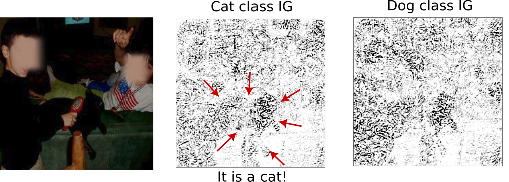
Despite the presence of noise in the outcomes, as depicted in Figure 2, these methods continue to find widespread application in fields like medicine [16]. Wang et al. [17] conducted an evaluation of three xAI methods – LRP, IG, and Guided Grad-CAM – in the context of MRI Alzheimer’s classification. They observed a substantial overlap among the three methods concerning brain regions, with IG showing the most promising results.

In fields like astronomy, gradient-based techniques are employed in research papers, such as the study conducted by Bhambra et al. [18] concerning galaxy topology classification. They applied SmoothGRAD [19] and found it to offer satisfactory explanations for their study.

Additionally, broader studies integrate gradient-based techniques in their investigations. Morrison et al. [20] utilize gradient methods to contrast attention-based models and CNN architectures with human perception. Woerl et al. [21] analyze and improve the robustness of saliency maps for data-driven explanations.

Given the prevalent application of these techniques, particularly in critical fields like medicine, we perceive an under-exploration concerning the interpretation of attribution maps derived from gradient-based methods. To address this gap, we introduce Gradient Artificial Distancing ($\mathrm{GAD}$), designed to emphasize in the attribution maps solely those image regions that significantly contribute to class differentiation. This approach aims to minimize noise, thereby enhancing human interpretability.

3 Intuition

Human perception tends to group nearby image pixels as a single entity, simplifying interpretation by reducing the number of components to analyze. Drawing clear boundaries around these components would ideally enhance the interpretability of the image.

However, when the selected pixels lack evident proximity, defining components becomes more challenging. Consider Figure 2 as an illustration, depicting important pixels in black within the second and third images. While there’s a concentrated region of pixels that might represent the cat, the majority of the images display scattered black pixels, complicating interpretation.

We believe that we can enhance the interpretability of an explanation by reducing the scattered important pixels (depicted in black) to form smaller and denser regions. However, merely applying an intensity-based filter in the explanation image is not sufficient to maintain the network’s accuracy. Such a filter would solely rely on an individual image each time, disregarding the network’s comprehensive knowledge.

Our idea is based on a premise: the final activations’ magnitudes in a network are inconsequential as long as, for the same set of images, the activations’ order remains consistent. In essence, consider two networks providing activations $(1,-1),(0.5,-0.6),(-0.9,0.8)$ for images $\mathbf{I}_{1},\mathbf{I}_{2}$, and $\mathbf{I}_{3}$, respectively, exhibiting a similar order of activations for each class individually as another network with activations $(1,-2),(0.5,-1.6),(-1.9,0.8)$. Both networks comprehend the three images similarly.

From the perspective of representation learning, this premise holds true as it maintains the spatial arrangement, preserving each image’s position relative to its neighbors (akin to a simple translation in space). Nevertheless, the second set of activations exhibits a more pronounced distinction between the two classes.

Our objective is to leverage this discrepancy between classes to minimize the number of image parts under scrutiny, emphasizing solely the most critical differences between classes, all while preserving the fidelity to the original model.

4 Gradient artificial distancing

To find these most important class differences, we worked on the class activations from the training samples. Consider a classification problem with $m$ classes ${\cal C}=\{c_{d}\}_{d=1}^{m}$, a dataset ${\cal D}=\bigcup\limits_{d=1}^{m}{\cal D}_{c_{d}}$, with $n_{d}$ samples ${\cal D}_{c_{d}}=\{\mathbf{I}_{c_{d},i}\}_{i=1}^{n_{d}}$ from the class $c_{d}$. Our goal is to accentuate class distinctions by artificially augmenting the disparity in final activations, effectively translating (distancing) the classes.

Our aim is to separate classes while preserving the original output space structure, maintaining the distribution of samples within the final activations’ space. This strategy compels the network to focus solely on image regions crucial for creating the gap between classes.

With this method, we want to ensure that:

• The updated activations’ output space can be approximated using the identical network architecture and the original model’s weights. Consequently, the optimization process aims to yield a close approximation with the initialization of the original weights.

• The final explanation is expected to have fewer highly important pixels, but it must not introduce new crucial pixels that were absent in the original explanation. Incorporating new important pixels would deviate the explanation from the knowledge embedded within the original model.

Three steps compose this process, as developed hereafter.

4.1 Choosing classes of interest to increase distances

We selected two specific classes from the set of trained classes, ${\cal C}$, with the aim of creating a distinct separation between them. For instance, consider the classes cat and dog. Our objective is to augment the separation by minimizing the likelihood of a dog being classified as a cat and vice-versa, all while maintaining the original learned structure.

We opted to modify the pre-Softmax activations instead of the post-Softmax ones to assess the increase in class separation, avoiding the normalization inherent in the Softmax function (which scales values between 0 and 1). Hence, we directly alter the non-normalized activations pertaining to the likelihood of an image being a dog within ${\cal D}{cat}$ (cat images) by subtracting a value $\alpha{cat}$. Similarly, we subtract a value $\alpha_{dog}$ from the probabilities of ${\cal D}_{dog}$ samples (dog images) being classified as cats, depicted in Figure 1a. This process aims to diminish the consideration of cats as dogs and vice-versa, all artificially manipulated for this analysis.

4.2 Training regressions

This artificial distancing process necessitates training new models to prompt the networks to generate these revised cat/dog output activations. These models are trained as regression problems, aiming to precisely obtain the altered artificial activations. While the inputs $x$ remain the images from ${\cal D}$ and the weights are based on the analyzed classification network for initialization, the expected outputs $y$ now represent the modified probabilities. The primary goal is not to achieve more generalized models; rather, it’s to attain the most accurate approximations to these new outputs, thereby discerning the persistently important features from the original explanation. To facilitate this, we replace the Softmax activation with a Linear one and employ Mean Squared Error (MSE) for regression training. Figure 1b illustrates this transformation in the model learning process, with labels converted into a probability vector.

4.3 Choosing important features

For precision in identifying crucial features, we propose iterating through steps 1 and 2 (Sections 4.1 and 4.2) multiple times, progressively increasing the values of $\alpha_{cat}$ and $\alpha_{dog}$. This process yields multiple trained regression networks. Upon their training, each network is subject to the chosen Gradient-based xAI method when examining images. The significant features extracted should mirror those of the original model under explanation. However, we anticipate that the consistently important features across all networks will hold greater significance in differentiating the two classes. Figure 3 illustrates the utilization of four support regression networks to delineate important regions. The analyzed image, in which Integrated Gradients (IG) was applied, was erroneously classified as a dog by the network.

Figure 3: Example of choosing important features. After training regression networks, we apply the IG method for each resulting model and both classes. The final attribution map includes only features present in all five attribution maps, the initial one (classification model analyzed), and the four support regression models. We obtain filtered attribution maps, including the regions of the image that most separate classes.

5 Metrics for evaluation

We propose to evaluate our method using two criteria: Complexity and Sensitivity.

Regarding complexity, our aim is to prioritize visualizations that are less complex, indicating reduced noise levels. In terms of sensitivity, we seek to assess the consequences of occluding essential features on the model’s output. We compare occluding important features identified by $\mathrm{GAD}$ (our method) against occluding the remaining important features – constituting a supplementary set found in the original explanation but absent in $\mathrm{GAD}$’s explanation. The anticipation is that with $\mathrm{GAD}$, fewer important features will be identified, potentially yielding a more pronounced impact on the output.

Figure 4: Example of convex hull applied to an attribution map. We involve with the convex-hull the pixels reaching more than $10\%$ of the highest importance according to the GAD – Guided Propagation attribution map.

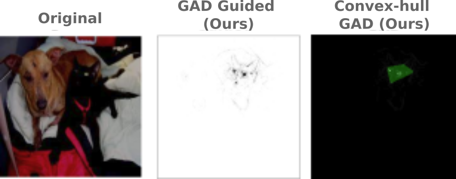
As mentioned earlier, we aim to simulate human perception, which tends to group nearby pixels as one unit. To account for this in our evaluation, we create a convex hull involving a selected set of the most important pixels. Figure 4 illustrates an instance of the produced convex hull. Therefore, concerning complexity, we assess the ratio $\mathit{RC}$ by comparing the area of the convex hull in the original explanation ($\mathit{A}(\mathit{CH}_{Orig})$) to the area of the convex hull in the $\mathrm{GAD}$ explanation ($\mathit{A}(\mathit{CH}_{{\mathrm{GAD}}})$):

$$\mathit{RC}=\frac{\mathit{A}(\mathit{CH}_{{\mathrm{GAD}}})}{\mathit{A}(\mathit{CH}_{Orig})}$$ (1)

where $0<\mathit{RC}<1.0$ represents a smaller important region for $\mathrm{GAD}$ explanation.

Regarding sensitivity, we leverage the created convex hulls to conduct occlusions. These convex hulls, denoted as $CH_{Orig}$ and $CH_{{\mathrm{GAD}}}$, are represented in image masks $\mathit{M}_{Orig}$ and $\mathit{M}_{{\mathrm{GAD}}}$, respectively, with a value of 1. Internal or boundary pixels within the convex hulls are assigned a value of 1, while the remaining pixels receive 0 (forming a binary mask). Utilizing these masks, we generate two occlusions: one using $\mathit{M}_{{\mathrm{GAD}}}$ and another employing $\mathit{M}_{Orig}-\mathit{M}_{{\mathrm{GAD}}}$. Our anticipation is that the occlusion using $\mathit{M}_{{\mathrm{GAD}}}$ will exert a more substantial impact.

To quantify this impact, we propose calculating the ratio $\mathit{RS}$, derived from the difference between the output before and after occlusion, divided by the area of the occluded section:

$$\mathit{RS}(\mathbf{I},\mathit{M},a)=\frac{|N_{a}(\mathbf{I})-N_{a}(\mathbf{I}\times(\mathbf{1}-\mathit{M}^{(a)}))|}{\sum_{i=0}^{m}\sum_{j=0}^{n}\mathit{M}_{i,j}^{(a)}}$$ (2)

where $N_{a}(\mathbf{I})$ is the output $a$ of the network for an image $\mathbf{I}\in{\cal D}$ of size $m\times n$ and $\mathit{M}_{i,j}^{(a)}$ is the pixel $(i,j)$ from a mask of size $m\times n$ corresponding to the output $a$. We expect $\mathit{RS}(\mathbf{I},\mathit{M}_{{\mathrm{GAD}}},a)>\mathit{RS}(\mathbf{I},\mathit{M}_{orig}-\mathit{M}_{{\mathrm{GAD}}},a),\forall a\in{\cal C}$ (for all classes).

6 Experiments and results

We experimented with two CNN architectures: VGG16 [22] and ResNet18 [12], utilizing two distinct datasets. The first dataset involves a binary classification of cats and dogs , while the second dataset, the CUB-200-2011 dataset [23], focuses on bird classification. For the bird classification task, we specifically chose the warbler and sparrow species as the two classes (the original dataset comprises 20 classes each, which we put together for this analysis).

We applied values $\alpha={0,2,4,6,8}$ for both classes. The support regression networks initiated the training using weights from the analyzed classification model (original model). Each support model underwent training for 10 epochs, utilizing the Adam optimizer and a learning rate set to $4\times 10^{-5}$.

In the subsequent experiments on complexity and sensitivity, we employed a total of 512 images (for both datasets), evenly distributed with 256 images per class. To create the convex hull, we filtered out $50\%$ of the pixels, retaining only the most important half.

6.1 Complexity

Following the computation of $\mathit{RC}$ (Equation 1) for all 512 images, we count the number of images where $\mathit{RC}<1.0$, indicating a point in favor of $\mathrm{GAD}$, and those where $\mathit{RC}\geq 1.0$, indicating a point in favor of the original visualization.

Table 1: For most methods, $\mathrm{GAD}$ is able to reduce interest area in visualizations. Evaluation of $\mathit{RC}$ for five literature methods, Saliency (S), Deconvolution (D), Gradient x Input (GxI), Guided-Backpropagation (GB) and Integrated Gradients (IG); two architectures, ResNet18 and VGG16; and two datasets, Cat x Dog and Birds. Orig.1 and Orig.2 represent the original methods’ visualization for the two classes. $\mathrm{GAD}$ 1 and $\mathrm{GAD}$ 2 are the application of our method to both classes visualizations.

			S	D	GxI	GB	IG
		Orig.1	357	0	15	4	17
		$\mathrm{GAD}$ 1 (ours)	155	512	490	427	480
		Orig.2	159	0	2	3	0
	VGG	$\mathrm{GAD}$ 2 (ours)	348	512	494	428	486
		Orig.1	122	0	2	10	7
		$\mathrm{GAD}$ 1 (ours)	390	512	492	453	497
		Orig.2	130	0	3	5	2
Cat x Dog	ResNet	$\mathrm{GAD}$ 2 (ours)	380	512	490	460	488
		Orig.1	270	0	9	0	1
		$\mathrm{GAD}$ 1 (ours)	240	511	488	450	500
		Orig.2	301	0	10	0	0
	VGG	$\mathrm{GAD}$ 2 (ours)	210	510	494	451	504
		Orig.1	153	0	1	0	0
		$\mathrm{GAD}$ 1 (ours)	358	512	504	472	506
		Orig.2	174	0	2	0	0
Birds	ResNet	$\mathrm{GAD}$ 2 (ours)	337	512	506	470	504

We show, in Table 1, the number of images where $\mathrm{GAD}$ (Ours) and the original method exhibited smaller complexity (smaller important areas). Through the experiments involving five literature methods – Saliency (S), Deconvolution (D), Gradient x Input (GxI), Guided-Backpropagation (GB), and Integrated Gradients (IG) – we observed that $\mathrm{GAD}$ successfully reduces the area of importance for nearly all images and methods.

6.2 Sensitivity

Upon computing $\mathit{RS}(\mathbf{I},\mathit{M},a)$ (Equation 2) for the four occlusion masks, which include two masks per class $a$ ($\mathit{M}_{{\mathrm{GAD}}}$ and $\mathit{M}_{Orig}-\mathit{M}_{{\mathrm{GAD}}}$), we acquire four respective $\mathit{RS}$ values each time. We designated the mask $\mathit{M}_{Orig}-\mathit{M}_{{\mathrm{GAD}}}$ as the supplementary mask, denoted as Sup., and $\mathit{M}_{{\mathrm{GAD}}}$ simply as $\mathrm{GAD}$. Therefore, the resulting four values correspond to: $\mathit{RS}(\mathbf{I},{\mathrm{GAD}}_{1},1)$, $\mathit{RS}(\mathbf{I},{\mathrm{GAD}}_{2},2)$, $\mathit{RS}(\mathbf{I},\mathit{Sup.}_{1},1)$, and $\mathit{RS}(\mathbf{I},\mathit{Sup.}_{2},2)$.

Table 2: Four out of five literature methods indicate a bigger impact when occluding the important regions found by $\mathrm{GAD}$. Evaluation of $\mathit{RS}$ for five literature methods, Saliency (S), Deconvolution (D), Gradient x Input (GxI), Guided-Backpropagation (GB) and Integrated Gradients (IG); two architectures, ResNet18 and VGG16; and two datasets, Cat x Dog and Birds. Sup.1, Sup.2, $\mathrm{GAD}$ 1, and $\mathrm{GAD}$ 2 indicate the average $\mathit{RS}$ values using these for different masks for occlusion. Sup.1 and Sup.2 represent the supplementary masks for the two classes. $\mathrm{GAD}$ 1 and $\mathrm{GAD}$ 2 are our method masks for both classes. Values in $10^{2}$ scale.

			S	D	GxI	GB	IG
		Sup.1	0.0800	0.0029	0.0052	0.1100	0.0100
		$\mathrm{GAD}$ 1 (ours)	0.1300	0.0056	0.1200	1.5900	0.1300
		Sup.2	0.2400	0.0029	0.0051	0.1500	0.0096
	VGG	$\mathrm{GAD}$ 2 (ours)	0.2500	0.0062	0.5600	1.8200	0.4900
		Sup.1	0.0600	0.0013	0.0016	0.1300	0.0016
		$\mathrm{GAD}$ 1 (ours)	0.0300	0.0024	0.0700	0.5100	0.1200
		Sup.2	0.0500	0.0012	0.0016	0.1000	0.0020
Cat x Dog	ResNet	$\mathrm{GAD}$ 2 (ours)	0.0700	0.0024	0.1600	0.4700	0.1600
		Sup.1	0.2500	0.0027	0.0800	0.0100	0.0100
		$\mathrm{GAD}$ 1 (ours)	0.2000	0.0056	0.5400	1.2800	0.5500
		Sup.2	0.1500	0.0030	0.0092	0.0100	0.0072
	VGG	$\mathrm{GAD}$ 2 (ours)	0.1300	0.0068	0.3600	1.4100	0.3800
		Sup.1	0.1100	0.0020	0.0045	0.0100	0.0094
		$\mathrm{GAD}$ 1 (ours)	0.0400	0.0048	0.1700	1.0300	0.2900
		Sup.2	0.0500	0.0019	0.0037	0.0100	0.0026
Birds	ResNet	$\mathrm{GAD}$ 2 (ours)	0.0500	0.0048	0.1600	1.0400	0.2000

We show, in Table 2, the average $\mathit{RS}$ values across all 512 images for $\mathrm{GAD}$ 1, $\mathrm{GAD}$ 2, Sup.1, and Sup.2, for the five literature methods, two architectures, and two datasets. For Deconvolution, Gradient x Input, Guided-Backpropagation, and Integrated Gradients, our method ($\mathrm{GAD}$) effectively identifies the most impactful regions for each decision, excluding the supplementary area (from the original visualization) that does not exhibit a greater impact (per pixel). However, in the case of Saliency visualization, both the areas selected by $\mathrm{GAD}$ and the supplementary areas display similar impacts, indicating limited benefits of our method for this particular technique.

6.3 $\mathrm{GAD}$ attribution maps

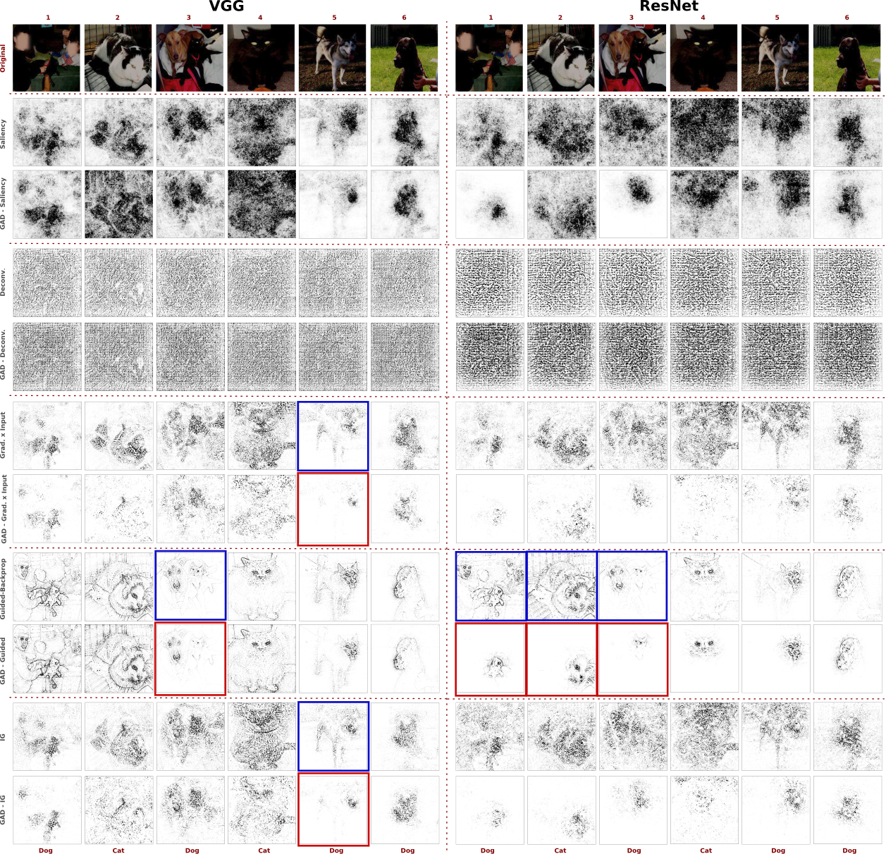
We present in Figure 5 the qualitative results of employing $\mathrm{GAD}$ with five gradient-based techniques. Each set of two rows illustrates the original attribution maps in the first row and the corresponding $\mathrm{GAD}$ maps in the second row. These pairs of rows represent the tested methods: Saliency, Deconvolution, Gradient x Input, Guided-Backpropagation, and Integrated Gradients. The results for VGG are displayed on the right side, while those for ResNet are on the left. The classification results (cat or dog) are presented at the bottom. Notable examples highlight the enhancements in visualizations: the original attribution maps are represented in blue, and the corresponding $\mathrm{GAD}$ visualizations are shown in red. For instance, Image 3 (highlighted in both networks) demonstrates a noteworthy distinction: both VGG and ResNet original attribution maps (in blue) appear similar in identifying the image as a dog. However, upon applying $\mathrm{GAD}$, distinct attribution maps (in red) emerge, with VGG focusing on the dog while ResNet emphasizes the cat, despite both networks classifying the image as a dog.

Figure 5: Our final visualizations: $\mathrm{GAD}$ improves interpretability of attribution maps. We present two-by-two rows of original attribution maps and $\mathrm{GAD}$ maps from five gradient-based techniques: Saliency, Deconvolution, Gradient x Input, Guided-Backpropagation, and Integrated Gradients. We present on the right side the VGG results and on the left side the ResNet ones. At the bottom, we present the obtained classification for each image (cat or dog).

6.4 Finding visual knowledge clues

Figure 6 illustrates a comparative visualization between original and GAD-interest areas. Aligned with the metrics detailed in Section 5, we generated the convex hulls involving the most important pixels per visualization. We show the five less activated images for each assigned class (original label), for VGG (on the right) and ResNet (on the left), within the bird dataset (at the top), and the cat vs. dog dataset (at the bottom). In these visualizations, the GAD-obtained regions are highlighted in green, while the original regions are marked in red. We expect small green regions.

Figure 6: Convex-hull comparisons for evaluation: The convex-hull of $\mathrm{GAD}$’s important features considerably reduces the images’ interest regions. The comparison between original and $\mathrm{GAD}$ convex hulls is able to give insights into why misclassifications happen. We show, in red, the original convex hull, and in green, the $\mathrm{GAD}$ convex hull, for the five literature techniques (IG, Guided-Backpropagation, Gradient x Input, Deconvolution, and Saliency), the two architectures and the two datasets. We chose to visualize the less activated images for the corresponding label class in each model.

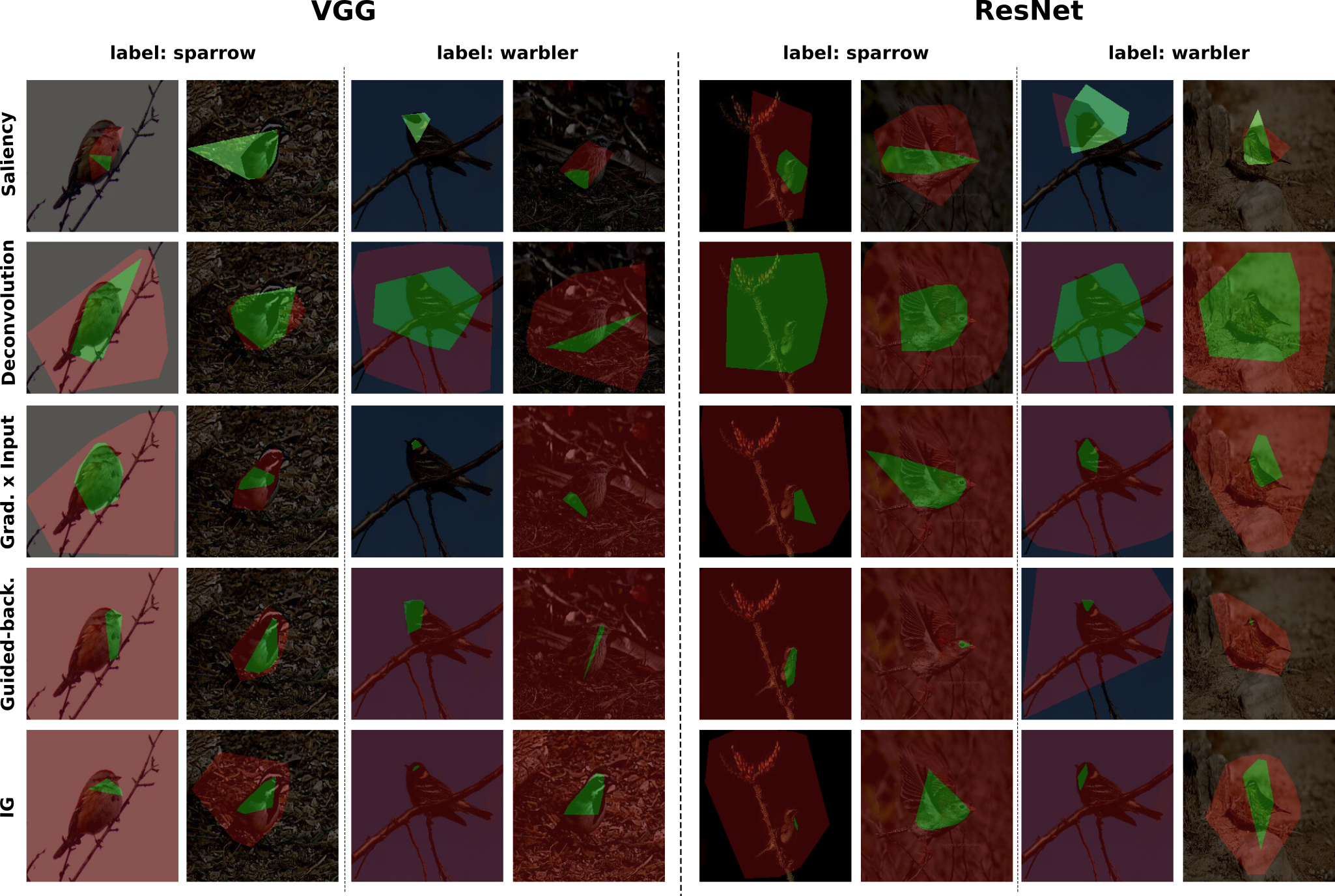
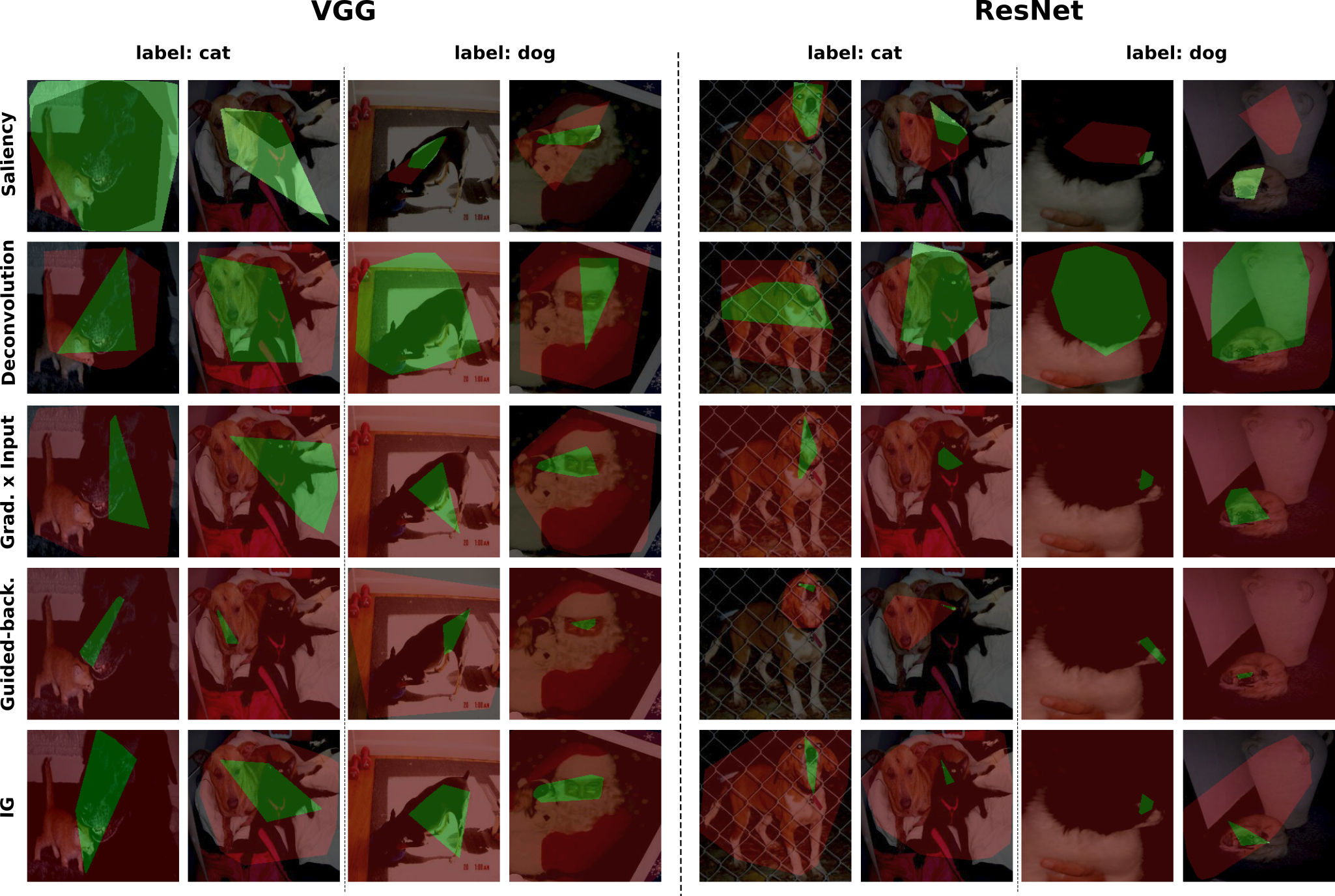
Additionally, we aimed to comprehend why these images were the least activated for their respective classes. While the bird dataset displays consistent behavior, the cat vs. dog dataset contains some images featuring both animals and occasionally people. Specifically, for VGG, the initial image showcases both animal types, with the dog (as per the larger green area) deemed more important than the cat. The final image features both a dog and Santa Claus, where both the animal and the person are deemed important. Regarding ResNet, the last image is intriguing as the dog is correctly identified as an important region, but the vase’s presence likely diminishes the dog’s activation for the dog class. In both models, the second-worst image is the same, containing both animal types, exemplifying differences between the models: VGG appears to recognize parts of both animal types, whereas ResNet emphasizes the cat, despite the dog’s prominence impacting the cat’s activation.

7 Conclusion

The experiments demonstrated that $\mathrm{GAD}$ effectively identifies the primary regions influencing class relationships. Through mask-based occlusions, it was observed that $\mathrm{GAD}$ can emphasize the most impactful region in decision-making, even when dealing with smaller significant areas. Across both datasets and models, $\mathrm{GAD}$ reduced complexity and enhanced the sensitivity of five gradient-based explainability techniques. These outcomes facilitated a deeper comprehension of the networks’ knowledge and provided insights into the causes behind certain misclassification errors. In future work, we aim to explore different values for $\alpha$ and devise methods for automatically selecting the optimal range of $\alpha$ values to maximize the impact of the support regression models.

References

- [1] D. Erhan, Y. Bengio, A. Courville, P. Vincent, Visualizing higher-layer features of a deep network, Technical Report, Univeristé de Montréal (2009) 1–13.
- [2] J. Bien, R. Tibshirani, Prototype selection for interpretable classification, Annals of Applied Statistics 5 (4) (2012) 1–23.
- [3] B. Kim, R. Khanna, O. Koyejo, Examples are not enough, learn to criticize! Criticism for interpretability, in: 30th International Conference on Neural Information Processing Systems (NeurIPS), 2016, pp. 2288–2296.
- [4] M. T. Ribeiro, S. Singh, C. Guestrin, ”Why Should I Trust You?”: Explaining the predictions of any classifier, in: 22nd International Conference on Knowledge Discovery and Data Mining (KDD), 2016, pp. 1135–1144.
- [5] J. J. Thiagarajan, B. Kailkhura, P. Sattigeri, K. N. Ramamurthy, Treeview: Peeking into deep neural networks via feature-space partitioning (2016).
- [6] K. Simonyan, A. Vedaldi, A. Zisserman, Deep inside convolutional networks: Visualising image classification models and saliency maps, in: Workshop at 2nd International Conference on Learning Representations (ICLR), 2014, pp. 1–8.
- [7] L. Merrick, Randomized ablation feature importance (2019).
- [8] M. D. Zeiler, R. Fergus, Visualizing and understanding convolutional networks, in: 13th European Conference on Computer Vision (ECCV), 2014, pp. 818–833.
- [9] S. Bach, A. Binder, G. Montavon, F. Klauschen, K.-R. Muller, W. Samek, On pixel-wise explanations for non-linear classifier decisions by layer-wise relevance propagation, PLoS One 10 (7) (2015) 1–46.
- [10] S. M. Lundberg, S.-I. Lee, A unified approach to interpreting model predictions, in: 31st International Conference on Neural Information Processing Systems (NeurIPS), 2017, pp. 4768–4777.
- [11] M. Sundararajan, A. Taly, Q. Yan, Axiomatic attribution for deep networks, in: 34th International Conference on Machine Learning (ICML), 2017, pp. 3319–3328.
- [12] K. He, X. Zhang, S. Ren, J. Sun, Deep residual learning for image recognition, in: 29th IEEE Conference on Computer Vision and Pattern Recognition (CVPR), 2016, pp. 770–778.
- [13] A. Adadi, M. Berrada, Peeking inside the black-box: A survey on explainable artificial intelligence (XAI), IEEE Access 6 (2018) 1–23.
- [14] A. Shrikumar, P. Greenside, A. Kundaje, Learning important features through propagating activation differences, in: 34th International Conference on Machine Learning (ICML), 2017, pp. 3145–3153.
- [15] J. T. Springenberg, A. Dosovitskiy, T. Brox, M. Riedmiller, Striving for simplicity: The all convolutional net, in: 3rd International Conference on Learning Representations (ICLR), 2015, pp. 1–14.
- [16] K. Borys, Y. A. Schmitt, M. Nauta, C. Seifert, N. Krämer, C. M. Friedrich, F. Nensa, Explainable ai in medical imaging: An overview for clinical practitioners – saliency-based xai approaches, European Journal of Radiology 162 (2023) 110787.
- [17] D. Wang, N. Honnorat, P. T. Fox, K. Ritter, S. B. Eickhoff, S. Seshadri, M. Habes, Deep neural network heatmaps capture alzheimer’s disease patterns reported in a large meta-analysis of neuroimaging studies, NeuroImage 269 (2023) 1–12.
- [18] P. Bhambra, B. Joachimi, O. Lahav, Explaining deep learning of galaxy morphology with saliency mapping, Monthly Notices of the Royal Astronomical Society 511 (4) (2022) 5032–5041.
- [19] D. Smilkov, N. Thorat, B. Kim, F. Viégas, M. Wattenberg, Smoothgrad: removing noise by adding noise, in: arXiv, 2017.
- [20] K. Morrison, A. Mehra, A. Perer, Shared interest…sometimes: Understanding the alignment between human perception, vision architectures, and saliency map techniques, in: IEEE/CVF Conference on Computer Vision and Pattern Recognition (CVPR) Workshops, 2023, pp. 3776–3781.
- [21] A.-C. Woerl, J. Disselhoff, M. Wand, Initialization noise in image gradients and saliency maps, in: IEEE/CVF Conference on Computer Vision and Pattern Recognition (CVPR), 2023, pp. 1766–1775.
- [22] K. Simonyan, A. Zisserman, Very deep convolutional networks for large-scale image recognition, in: 3rd International Conference on Learning Representations (ICLR), 2015.
- [23] X. He, Y. Peng, Fine-grained visual-textual representation learning, IEEE Transactions on Circuits and Systems for Video Technology PP (2019) 1–12.