Fundamental Convergence Analysis of Sharpness-Aware Minimization

Abstract

The paper investigates the fundamental convergence properties of Sharpness-Aware Minimization (SAM), a recently proposed gradient-based optimization method (Foret et al., 2021) that significantly improves the generalization of deep neural networks. The convergence properties including the stationarity of accumulation points, the convergence of the sequence of gradients to the origin, the sequence of function values to the optimal value, and the sequence of iterates to the optimal solution are established for the method. The universality of the provided convergence analysis based on inexact gradient descent frameworks (Khanh et al., 2023b) allows its extensions to the normalized versions of SAM such as VaSSO (Li & Giannakis, 2023), RSAM (Liu et al., 2022), and to the unnormalized versions of SAM such as USAM (Andriushchenko & Flammarion, 2022). Numerical experiments are conducted on classification tasks using deep learning models to confirm the practical aspects of our analysis.

1 Introduction

This paper concentrates on optimization methods for solving the standard unconstrained optimization problem

$${\rm minimize}\quad f(x)\text{ subject to }x\in{\rm I\!R}^{n},$$ (1)

where $f:{\rm I\!R}^{n}\rightarrow{\rm I\!R}$ is a continuously differentiable ($\mathcal{C}^{1}$-smooth) function. We study the convergence behavior of the gradient-based optimization algorithm Sharpness-Aware Minimization (Foret et al., 2021) together with its efficient practical variants (Liu et al., 2022; Li & Giannakis, 2023; Andriushchenko & Flammarion, 2022). Given an initial point $x^{1}\in{\rm I\!R}^{n},$ the original iterative procedure of SAM is designed as follows

$$\quad x^{k+1}=x^{k}-t\nabla f\left(x^{k}+\rho\frac{\nabla f(x^{k})}{\left\|\nabla f(x^{k})\right\|}\right)$$ (2)

for all $k\in{\rm I\!N}$, where $t>0$ and $\rho>0$ are respectively the stepsize (in other words, the learning rate) and perturbation radius. The main motivation for the construction algorithm is that by making the backward step $x^{k}+\rho\frac{\nabla f(x^{k})}{\left\|\nabla f(x^{k})\right\|}$, it avoids minimizers with large sharpness, which is usually poor for the generalization of deep neural networks as shown in (Keskar et al., 2017).

1.1 Lack of convergence properties for SAM due to constant stepsize

The consistently high efficiency of SAM has driven a recent surge of interest in the analysis of the method. The convergence analysis of SAM is now a primary focus on its theoretical understanding with several works being developed recently (e.g., Ahn et al. (2023); Andriushchenko & Flammarion (2022); Dai et al. (2023); Si & Yun (2023)). However, none of the aforementioned studies have addressed the fundamental convergence properties of SAM, which are outlined below where the stationary accumulation point in (2) means that every accumulation point $\bar{x}$ of the iterative sequence $\left\{x^{k}\right\}$ satisfies the condition $\nabla f(\bar{x})=0$.

(1)	$\displaystyle{\liminf_{k\rightarrow\infty}}\left\|\nabla f(x^{k})\right\|=0$
(2)	stationary accumulation point
(3)	$\displaystyle{\lim_{k\rightarrow\infty}}\left\|\nabla f(x^{k})\right\|=0$
(4)	$\displaystyle{\lim_{k\rightarrow\infty}}f(x^{k})=f(\bar{x})$ with $\nabla f(\bar{x})=0$
(5)	$\left\{x^{k}\right\}$ converges to some $\bar{x}$ with $\nabla f(\bar{x})=0$

Table 1: Fundamental convergence properties of smooth optimization methods

The relationship between the properties above is summarized as follows:

(1)$\overset{\left\{\left\|x^{k}\right\|\right\}\not\rightarrow\infty}{\Longleftarrow}$ (2) $\Longleftarrow$ (3) $\Longleftarrow$ (5) $\Longrightarrow$ (4).

The aforementioned convergence properties are standard and are analyzed by various smooth optimization methods including gradient descent-type methods, Newton-type methods, and their accelerated versions together with nonsmooth optimization methods under the usage of subgradients. The readers are referred to Bertsekas (2016); Nesterov (2018); Polyak (1987) and the references therein for those results. The following recent publications have considered various types of convergence rates for the sequences generated by SAM as outlined below:

(i) Dai et al. (2023, Theorem 1)

$$f(x^{k})-f^{*}\leq(1-t\mu(2-Lt))^{k}(f(x^{0})-f^{*})+\frac{tL^{2}\rho^{2}}{2\mu(2-Lt)}$$

where $L$ is the Lipschitz constant of $\nabla f$, and where $\mu$ is the constant of strong convexity constant for $f$.

(ii) Si & Yun (2023, Theorems 3.3, 3.4)

$$\frac{1}{k}\sum_{i=1}^{k}\left\|\nabla f(x^{i})\right\|^{2} =\mathcal{O}\left(\frac{1}{k}+\frac{1}{\sqrt{k}}\right)$$

$$\frac{1}{k}\sum_{i=1}^{k}\left\|\nabla f(x^{i})\right\|^{2} =\mathcal{O}\left(\frac{1}{k}\right)+L^{2}\rho^{2},$$

where $L$ is the Lipschitz constant of $\nabla f.$ We emphasize that none of the results mentioned above achieve any fundamental convergence properties listed in Table 1. The estimation in (i) only gives us the convergence of the function value sequence to a value close to the optimal one, not the convergence to exactly the optimal value. Additionally, it is evident that the results in (ii) do not imply the convergence of $\left\{\nabla f(x^{k})\right\}$ to $0$. To the best of our knowledge, the only work concerning the fundamental convergence properties listed in Table 1 is Andriushchenko & Flammarion (2022). However, the method analyzed in that paper is unnormalized SAM (USAM), a variant of SAM with the norm being removed in the iterative procedure (1b). Recently, Dai et al. (2023) suggested that USAM has different effects in comparison with SAM in both practical and theoretical situations, and thus, they should be addressed separately. This observation once again highlights the necessity for a fundamental convergence analysis of SAM and its normalized variants.

Note that, using exactly the iterative procedure (2), SAM does not achieve the convergence for either $\left\{x^{k}\right\}$, or $\left\{f(x^{k})\right\}$, or $\left\{\nabla f(x^{k})\right\}$ to the optimal solution, the optimal value, and the origin, respectively. It is illustrated by Example 3.1 below dealing with the simple function $f(x):=x^{2}$. This calls for the necessity of employing an alternative stepsize rule for SAM. Scrutinizing the numerical experiments conducted for SAM and its variants (e.g., Foret et al. (2021, Subsection C1), Li & Giannakis (2023, Subsection 4.1)), we can observe that in fact the constant stepsize rule is not a preferred strategy. Instead, the cosine stepsize scheduler from (Loshchilov & Hutter, 2016), designed to decay to zero and then restart after each fixed cycle, emerges as a more favorable approach. This observation motivates us to analyze the method under the following diminishing stepsize:

$$\sum_{k=1}^{\infty}t_{k}=\infty\;\text{ and }\;\sum_{k=1}^{\infty}t_{k}^{2}<\infty.$$ (3)

This type of stepsize is employed in many optimization methods including the classical gradient descent methods together with its incremental and stochastic counterparts (Bertsekas & Tsitsiklis, 2000). The second condition in (3) also yields $t_{k}\downarrow 0,$ which is satisfied for the cosine stepsize scheduler in each cycle.

1.2 Our Contributions

Convergence of SAM and normalized variants

We establish fundamental convergence properties of SAM in various settings. In the convex case, we consider the perturbation radii to be variable and bounded. This analysis encompasses the practical implementation of SAM with a constant perturbation radius. The results in this case are summarized in Table 2.

Classes of function	Results
General setting	$\liminf\nabla f(x^{k})=0$
Bounded minimizer set	stationary accumulation point
Unique minimizer	$\left\{x^{k}\right\}$ is convergent

Table 2: Convergence properties of SAM for convex functions in Theorem 3.2

In the nonconvex case, we generally consider any variants of SAM, where the term $\frac{\nabla f(x^{k})}{\left\|\nabla f(x^{k})\right\|}$ is replaced by $\frac{d^{k}}{\left\|d^{k}\right\|}$ for any arbitrary $d^{k}\in{\rm I\!R}^{n}\setminus\left\{0\right\}$. This encompasses, in particular, recent developments named VaSSO (Li & Giannakis, 2023) and RSAM (Liu et al., 2022). To achieve this, we consider the perturbation radii to be variable. Although such a relaxation does not cover the constant case theoretically, it poses no harm in the practical implementation of the methods as discussed in Remark 3.7. The summary of our results in the nonconvex case is as follows.

Classes of function	Results
General setting	$\lim\nabla f(x^{k})=0$
General setting	$\lim f(x^{k})=f^{*}$
KL property	$\left\{x^{k}\right\}$ is convergent

Table 3: Convergence properties of in Theorem 3.3 addressing SAM and VaSSO for nonconvex functions

Convergence of USAM and unnormalized variants

Our last theoretical contribution in this paper involves a refined convergence analysis of USAM in Andriushchenko & Flammarion (2022). In the general setting, we address functions satisfying the $L$-descent condition (5), which is even weaker than the Lipschitz continuity of $\nabla f$ as considered in Andriushchenko & Flammarion (2022). The summary of the convergence analysis for USAM is as follows.

Classes of function	Results
General setting	stationary accumulation point
General setting	$\lim f(x^{k})=f^{*}$
$\nabla f$ is Lipschitz	$\lim\nabla f(x^{k})=0$
KL property	$\left\{x^{k}\right\}$ is convergent

Table 4: Convergence properties of USAM in Theorem 4.1

As discussed in Remark D.4, our convergence properties for USAM use weaker assumptions and cover a broader range of applications in comparison with those analyzed in (Andriushchenko & Flammarion, 2022). Furthermore, the universality of the conducted analysis allows us to verify all the convergence properties for the extragradient method (Korpelevich, 1976) that has been recently applied in (Lin et al., 2020) to large-batch training in deep learning.

1.3 Importance of Our Work

Our work develops, for the first time in the literature, a fairly comprehensive analysis of the fundamental convergence properties of SAM and its variants. The developed approach addresses general frameworks while being based on the analysis of the newly proposed inexact gradient descent methods. Such an approach can be applied in various other circumstances and provides useful insights into the convergence understanding of not only SAM and related methods but also many other numerical methods in smooth, nonsmooth, and derivative-free optimization.

1.4 Related Works

Variants of SAM. There have been several publications considering some variants to improve the performance of SAM. Namely, Kwon et al. (2021) developed the Adaptive Sharpness-Aware Minimization (ASAM) method by employing the concept of normalization operator. Du et al. (2022) proposed the Efficient Sharpness-Aware Minimization (ESAM) algorithm by combining stochastic weight perturbation and sharpness-sensitive data selection techniques. Liu et al. (2022) proposed a novel Random Smoothing-Based SAM method called RSAM that improves the approximation quality in the backward step. Quite recently, Li & Giannakis (2023) proposed another approach called Variance Suppressed Sharpness-aware Optimization (VaSSO), which perturbed the backward step by incorporating information from the previous iterations.

Theoretical Understanding of SAM. Despite the success of SAM in practice, a theoretical understanding of SAM was absent until several recent works. Barlett et al. (2023) analyzed the convergence behavior of SAM for convex quadratic objectives, showing that for most random initialization, it converges to a cycle that oscillates between either side of the minimum in the direction with the largest curvature. Ahn et al. (2023) introduces the notion of $\varepsilon$-approximate flat minima and investigates the iteration complexity of optimization methods to find such approximate flat minima. As discussed in Subsection 1.1, Dai et al. (2023) considers the convergence of SAM with constant stepsize and constant perturbation radius for convex and strongly convex functions, showing that the sequence of iterates stays in a neighborhood of the global minimizer while (Si & Yun, 2023) considered the properties of the gradient sequence generated by SAM in different settings.

Theoretical Understanding of USAM. This method was first proposed by Andriushchenko & Flammarion (2022) with fundamental convergence properties being analyzed under different settings of convex and nonconvex and optimization. Analysis of USAM was further conducted in Behdin & Mazumder (2023) for a linear regression model, and in Agarwala & Dauphin (2023) for a quadratic regression model. Detailed comparison between SAM and USAM, which indicates that they exhibit different behaviors, was presented in the two recent studies by Compagnoni et al. (2023) and Dai et al. (2023).

1.5 Contents

The rest of this paper is organized as follows. Section 2 presents some basic definitions and preliminaries used throughout the entire paper. The convergence properties of SAM along with its normalized variants are presented in Section 3, while those of USAM, along with its unnormalized variants, are presented in Section 4. Section 5 illustrates the results of numerical experiments comparing SAM with the cases of diminishing stepsize and constant stepsize. Section 6 discusses conclusions and limitations of our work and also outlines our future research in this direction. Due to the space limitation, technical proofs, additional remarks, and examples are deferred to the appendix.

2 Preliminaries

First we recall some notions and notations frequently used in the paper. All our considerations are given in the space ${\rm I\!R}^{n}$ with the Euclidean norm $\|\cdot\|$. As always, ${\rm I\!N}:=\{1,2,\ldots\}$ signifies the collections of natural numbers. The symbol $x^{k}\stackrel{{\scriptstyle J}}{{\to}}\bar{x}$ means that $x^{k}\to\bar{x}$ as $k\to\infty$ with $k\in J\subset{\rm I\!N}$. Recall that $\bar{x}$ is a stationary point of a $\mathcal{C}^{1}$-smooth function $f\colon{\rm I\!R}^{n}\rightarrow{\rm I\!R}$ if $\nabla f(\bar{x})=0$. A function $f:{\rm I\!R}^{n}\rightarrow{{\rm I\!R}}$ is said to posses a Lipschitz continuous gradient with the uniform constant $L>0$, or equivalently it belongs to the class $\mathcal{C}^{1,L}$, if we have the estimate

$$\left\|\nabla f(x)-\nabla f(y)\right\|\leq L\left\|x-y\right\|\;\text{ for all }\;x,y\in{\rm I\!R}^{n}.$$ (4)

This class of function enjoys the following property called the $L$-descent condition (see, e.g., Izmailov & Solodov (2014, Lemma A.11) and Bertsekas (2016, Lemma A.24)):

$$f(y)\leq f(x)+\left\langle\nabla f(x),y-x\right\rangle+\dfrac{L}{2}\left\|y-x\right\|^{2}$$ (5)

for all $x,y\in{\rm I\!R}^{n}.$ Conditions (4) and (5) are equivalent to each other when $f$ is convex, while the equivalence fails otherwise. A major class of functions satisfying the $L$-descent condition but not having the Lipschitz continuous gradient is given by Khanh et al. (2023b, Section 2) as

$$f(x):=\dfrac{1}{2}\left\langle Ax,x\right\rangle+\left\langle b,x\right\rangle+c-h(x),$$

where $A$ is an $n\times n$ matrix, $b\in{\rm I\!R}^{n}$, $c\in{\rm I\!R}$ and $h:{\rm I\!R}^{n}\rightarrow{\rm I\!R}$ is a smooth convex function whose gradient is not Lipschitz continuous. There are also circumstances where a function has a Lipschitz continuous gradient and satisfies the descent condition at the same time, but the Lipschitz constant is larger than the one in the descent condition.

Our convergence analysis of the methods presented in the subsequent sections benefits from the Kurdyka-Łojasiewicz $(KL)$ property taken from Attouch et al. (2010).

Definition 2.1 (Kurdyka-Łojasiewicz property).

We say that a smooth function $f:{\rm I\!R}^{n}\rightarrow{{\rm I\!R}}$ enjoys the KL property at $\bar{x}\in\mbox{\rm dom}\,\partial f$ if there exist $\eta\in(0,\infty]$, a neighborhood $U$ of $\bar{x}$, and a desingularizing concave continuous function $\varphi:[0,\eta)\rightarrow[0,\infty)$ such that:

(i) $\varphi(0)=0$.

(ii) $\varphi$ is $\mathcal{C}^{1}$-smooth on $(0,\eta)$.

(iii) $\varphi^{\prime}>0$ on $(0,\eta)$.

(iv) For all $x\in U$ with $0<f(x)-f(\bar{x})<\eta$, we have

$$\varphi^{\prime}(f(x)-f(\bar{x}))\left\|\nabla f(x)\right\|\geq 1.$$ (6)

Remark 2.2.

It has been realized that the KL property is satisfied in broad settings. In particular, it holds at every nonstationary point of $f$; see Attouch et al. (2010, Lemma 2.1 and Remark 3.2(b)). Furthermore, it is proved at the seminal paper Łojasiewicz (1965) that any analytic function $f:{\rm I\!R}^{n}\rightarrow{\rm I\!R}$ satisfies the KL property at every point $\bar{x}$ with $\varphi(t)~{}=~{}Mt^{1-q}$ for some $q\in[0,1)$. Typical functions that satisfy the KL property are semi-algebraic functions and also those from the more general class of functions known as definable in o-minimal structures; see Attouch et al. (2010, 2013); Kurdyka (1998).

We utilize the following assumption on the desingularizing function in Definition 2.1, which is employed in (Li et al., 2023). The satisfaction of this assumption for a general class of desingularizing functions is discussed in Remark D.1.

Assumption 2.3.

There is some $C>0$ such that

$$C[\varphi^{\prime}(x+y)]^{-1}\leq(\varphi^{\prime}(x))^{-1}+(\varphi^{\prime}(y))^{-1}$$

whenever $x,y\in(0,\eta)$ with $x+y<\eta.$

3 SAM and normalized variants

3.1 Convex case

We begin this subsection with an example that illustrates SAM’s inability to achieve the convergence of the sequence of iterates to an optimal solution by using a constant stepsize. This phenomenon persists even when considering basic functions with favorable geometric properties such as strongly convex quadratic functions; e.g., $f(x)=x^{2}$. This emphasizes the necessity of employing diminishing stepsizes in our subsequent analysis.

Example 3.1 (SAM with constant stepsize and constant perturbation radius does not converge).

Let the sequence $\left\{x^{k}\right\}$ be generated by SAM in (2) with any fixed small constant perturbation radius and constant stepsize together with an initial point close to $0$. Then the sequence $\left\{x^{k}\right\}$ generated by this algorithm does not converge to $0$.

The details of the above example are presented in Appendix A.1. Figure 1 gives an empirical illustration for Example 3.1. The graph shows that, while the sequence generated by GD converges to $0$, the one generated by SAM gets stuck at a different point.

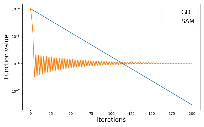
Figure 1: SAM with constant stepsize does not converge to optimal solution

The following result provides the convergence properties of SAM in the convex case.

Theorem 3.2.

Let $f:{\rm I\!R}^{n}\rightarrow{\rm I\!R}$ be a smooth convex function whose gradient is Lipschitz continuous with constant $L>0$. Given any initial point $x^{1}\in{\rm I\!R}^{n}$, let $\left\{x^{k}\right\}$ be generated by the SAM method with the iterative procedure

$$x^{k+1}=x^{k}-t_{k}\nabla f\left(x^{k}+\rho_{k}\frac{\nabla f(x^{k})}{\left\|\nabla f(x^{k})\right\|}\right)$$ (7)

for all $k\in{\rm I\!N}$ with nonnegative stepsizes and perturbation radii satisfying the conditions

$$\sum_{k=1}^{\infty}t_{k}^{2}<\infty,\;\sum_{k=1}^{\infty}t_{k}=\infty,\;\sup_{k\in{\rm I\!N}}\rho_{k}<\infty.$$ (8)

Assume that $\nabla f(x^{k})\neq 0$ for all $k\in{\rm I\!N}$ and that $\inf_{k\in{\rm I\!N}}f(x^{k})>-\infty$. Then the following assertions hold:

(i) $\displaystyle{\liminf_{k\rightarrow\infty}}\;\nabla f(x^{k})=0$.

(ii) If $f$ has a nonempty bounded level set, then $\left\{x^{k}\right\}$ is bounded, every accumulation point of $\left\{x^{k}\right\}$ is a global minimizer of $f$, and $\left\{f(x^{k})\right\}$ converges to the optimal value of $f$. If in addition $f$ has a unique minimizer, then the sequence $\left\{x^{k}\right\}$ converges to that minimizer.

The proof of the theorem is presented in Appendix C.1.

3.2 Nonconvex case

In this subsection, we study the convergence of several versions of SAM from the perspective of the inexact gradient descent methods.

Algorithm 1 Inexact Gradient Descent (IGD) Methods

Step 0.

Choose some initial point $x^{0}\in{\rm I\!R}^{n},$ sequence of errors $\left\{\varepsilon_{k}\right\}\subset(0,\infty)$, and sequence of stepsizes $\left\{t_{k}\right\}\subset(0,\infty).$ For $k=1,2,\ldots,$ do the following

Step 1.

Set $x^{k+1}=x^{k}-t_{k}g^{k}$ with $\left\|g^{k}-\nabla f(x^{k})\right\|\leq\varepsilon_{k}$.

This algorithm is motivated by while being different from the Inexact Gradient Descent methods proposed in (Khanh et al., 2023b, 2024, a, c). The latter constructions consider relative errors in gradient calculation, while Algorithm 1 uses the absolute ones. This approach is particularly suitable for the constructions of SAM and its normalized variants. The convergence properties of Algorithm 1 are presented in the next theorem.

Theorem 3.3.

Let $f:{\rm I\!R}^{n}\rightarrow{\rm I\!R}$ be a smooth function whose gradient is Lipschitz continuous with some constant $L>0$, and let $\left\{x^{k}\right\}$ be generated by the IGD method in Algorithm 1 with stepsizes and errors satisfying the conditions

$$\sum_{k=1}^{\infty}t_{k}=\infty,\;t_{k}\downarrow 0,\sum_{k=1}^{\infty}t_{k}\varepsilon_{k}<\infty,\;\limsup\varepsilon_{k}<2.$$ (9)

Assume that $\inf_{k\in{\rm I\!N}}f(x^{k})>-\infty$. Then the following convergence properties hold:

(i) $\nabla f(x^{k})\rightarrow 0,$ and thus every accumulation point of the iterative sequence $\left\{x^{k}\right\}$ is stationary for $f.$

(ii) If $\bar{x}$ is an accumulation point of the sequence $\left\{x^{k}\right\}$, then $f(x^{k})\rightarrow f(\bar{x}).$

(iii) Suppose that $f$ satisfies the KL property at some accumulation point $\bar{x}$ of $\left\{x^{k}\right\}$ with the desingularizing function $\varphi$ satisfying Assumption 2.3. Assume in addition that

$$\sum_{k=1}^{\infty}t_{k}\left(\varphi^{\prime}\left(\sum_{i=k}^{\infty}t_{k}\varepsilon_{k}\right)\right)^{-1}<\infty,$$ (10)

and that $f(x^{k})>f(\bar{x})$ for sufficiently large $k\in\mathbb{N}$. Then $x^{k}\rightarrow\bar{x}$ as $k\rightarrow\infty$. In particular, if $\bar{x}$ is a global minimizer of $f$, then either $f(x^{k})=f(\bar{x})$ for some $k\in\mathbb{N}$, or $x^{k}\rightarrow\bar{x}$.

The proof of the theorem is presented in Appendix C.2. The demonstration that condition (10) is satisfied when $\varphi(t)=Mt^{1-q}$ with some $M>0$ and $q\in(0,1)$, and when $t_{k}=\frac{1}{k}$ and $\varepsilon_{k}=\frac{1}{k^{p}}$ with $p\geq 0$ for all $k\in\mathbb{N}$, is provided in Remark D.3. It is worth noting that all the assumptions in Theorem 3.3(iii) are fulfilled if, in particular, the function $f$ satisfies the Polyak-Łojasiewicz inequality (Polyak, 1987). This inequality is another standard assumption used in the convergence analysis of various optimization methods in machine learning (Karimi et al., 2016).

The next example discusses the necessity of the last two conditions in (9) in the convergence analysis of IGD while demonstrating that employing a constant error leads to the convergence to a nonstationary point of the method.

Example 3.4 (IGD with constant error converges to a nonstationary point).

Let $f:{\rm I\!R}\rightarrow{\rm I\!R}$ be defined by $f(x)=x^{2}$ for $x\in{\rm I\!R}$. Given a perturbation radius $\rho>0$ and an initial point $x^{1}>\rho$, consider the iterative sequence

$$x^{k+1}=x^{k}-2t_{k}\left(x^{k}-\rho\frac{x^{k}}{|x^{k}|}\right)\;\text{ for }k\in{\rm I\!N},$$ (11)

where $\left\{t_{k}\right\}\subset[0,1/2],t_{k}\downarrow 0,$ and $\sum_{k=1}^{\infty}t_{k}=\infty$. This algorithm is in fact the IGD applied to $f$ with $g^{k}=\nabla f\left(x^{k}-\rho\frac{f^{\prime}(x^{k})}{\left|f^{\prime}(x^{k})\right|}\right)$. Then $\left\{x^{k}\right\}$ converges to $\rho,$ which is not a stationary point of $f.$

The details of the example are presented in Appendix A.2.

We now propose a general framework that encompasses SAM and all of its normalized variants including RSAM in Liu et al. (2022) and VaSSO in Li & Giannakis (2023).

Algorithm 1a General framework for normalized variants of SAM

Step 0.

Choose some initial point $x^{1}\in{\rm I\!R}^{n},$ sequence of perturbation radii $\left\{\rho_{k}\right\}\subset(0,\infty)$, and sequence of stepsizes $\left\{t_{k}\right\}\subset(0,\infty).$ For $k=1,2,\ldots,$ do the following:

Step 1.

Choose some $d^{k}\in{\rm I\!R}^{n}\setminus\left\{0\right\}.$

Step 2.

Set $x^{k+1}=x^{k}-t_{k}\nabla f\left(x^{k}+\rho_{k}\frac{d^{k}}{\left\|d^{k}\right\|}\right)$.

Algorithm 1b (Foret et al., 2021) Sharpness-Aware Minimization (SAM)

Step 0.

Choose some initial point $x^{1}\in{\rm I\!R}^{n},$ sequence of perturbation radii $\left\{\rho_{k}\right\}\subset[0,\infty)$, and sequence of stepsizes $\left\{t_{k}\right\}\subset[0,\infty).$ For $k=1,2,\ldots,$ do the following:

Step 1.

Set $x^{k+1}=x^{k}-t_{k}\nabla f\left(x^{k}+\rho_{k}\frac{\nabla f(x^{k})}{\left\|\nabla f(x^{k})\right\|}\right)$.

Algorithm 1c (Liu et al., 2022) Random Sharpness-Aware Minimization (RSAM)

Step 0.

Choose some initial point $x^{1}\in{\rm I\!R}^{n},$ sequence of perturbation radii $\left\{\rho_{k}\right\}\subset[0,\infty)$, and sequence of stepsizes $\left\{t_{k}\right\}\subset[0,\infty).$ For $k=1,2,\ldots,$ do the following:

Step 1.

Construct a random vector $\Delta^{k}\in{\rm I\!R}^{n}$ and set $g^{k}=\nabla f(x^{k}+\Delta^{k}).$

Step 2.

Set $x^{k+1}=x^{k}-t_{k}\nabla f\left(x^{k}+\rho_{k}\frac{\delta^{k}+\lambda g^{k}}{\left\|\delta^{k}+\lambda g^{k}\right\|}\right)$.

Algorithm 1d (Li & Giannakis, 2023) Variance suppressed sharpness aware optimization (VaSSO)

Step 0.

Choose some initial point $x^{1}\in{\rm I\!R}^{n}$, initial direction $d^{1}\in{\rm I\!R}^{n}$, sequence of perturbation radii $\left\{\rho_{k}\right\}\subset[0,\infty)$, and sequence of stepsizes $\left\{t_{k}\right\}\subset[0,\infty).$ For $k=1,2,\ldots,$ do the following:

Step 1.

Set $d^{k+1}=(1-\theta)d^{k}+\theta\nabla f(x^{k}).$

Step 2.

Set $x^{k+1}=x^{k}-t_{k}\nabla f\left(x^{k}+\rho_{k}\frac{d^{k}}{\left\|d^{k}\right\|}\right).$

Remark 3.5.

It is clear that Algorithms 1b-1d are specializations of Algorithm 1a with $d^{k}=\nabla f(x^{k})$ in Algorithm 1b, $d^{k}=\delta^{k}+\lambda g^{k}$ in Algorithm 1c, and $d^{k}$ constructed inductively in Step 1 of Algorithm 1d. We show that Algorithm 1a is in turn a special case of IGD in Algorithm 1, and it thus achieves all the convergence properties in Theorem 3.3.

Corollary 3.6.

Let $f:{\rm I\!R}^{n}\rightarrow{\rm I\!R}$ be a $\mathcal{C}^{1,L}$ function, and let $\left\{x^{k}\right\}$ be generated by Algorithm 1a with the parameters

$$\sum_{k=1}^{\infty}t_{k}=\infty,\;t_{k}\downarrow 0,\sum_{k=1}^{\infty}t_{k}\rho_{k}<\infty,\;\limsup\rho_{k}<\frac{2}{L}.$$ (12)

Assume that $\inf_{k\in{\rm I\!N}}f(x^{k})>-\infty$. Then all the convergence properties presented in Theorem 3.3 hold.

Proof.

Considering Algorithm 1a and defining $g^{k}=\nabla f\left(x^{k}+\rho_{k}\frac{d^{k}}{\left\|d^{k}\right\|}\right)$, we deduce that

$$\left\|g^{k}-\nabla f(x^{k})\right\|\leq L\left\|x^{k}+\rho_{k}\frac{d^{k}}{\left\|d^{k}\right\|}-x^{k}\right\|=L\rho_{k}.$$

Therefore, Algorithm 1a is a specialization of Algorithm 1 with $\varepsilon_{k}=L\rho_{k}.$ Combining this with (12) also gives us (9), thereby verifying all the assumptions in Theorem 3.3. Consequently, all the convergence properties outlined in Theorem 3.3 hold for Algorithm 1a. ∎

Remark 3.7.

Note that the conditions in (12) do not pose any obstacles to the implementation of a constant perturbation radius for SAM in practical deep neural networks. For example, a possible selection of ${t_{k}}$ and ${\rho_{k}}$ that satisfy (12) is $t_{k}=\frac{1}{k}$ and $\rho_{k}=\frac{1}{k^{0.001}}$ for all $k\in{\rm I\!N}$. Then the initial perturbation radius is $1$, while that after 1 million iterations is still greater than $0.99$. In general, the conditions in (12) do not require the convergence of $\left\{\rho_{k}\right\}$ to $0,$ which is discussed in Remark D.2.

4 USAM and unnormalized variants

In this section, we study the convergence of various versions of USAM from the perspective of the following Inexact Gradient Descent method with relative errors.

Algorithm 2 IGDr

Step 0.

Choose some initial point $x^{0}\in{\rm I\!R}^{n},$ a relative error $\nu\geq 0$, and a sequence of stepsizes $\left\{t_{k}\right\}\subset[0,\infty).$ For $k=1,2,\ldots,$ do the following:

Step 1.

Set $x^{k+1}=x^{k}-t_{k}g^{k}$, where $\left\|g^{k}-\nabla f(x^{k})\right\|\leq\nu\left\|\nabla f(x^{k})\right\|$.

This algorithm was initially introduced in Khanh et al. (2023b) in a different form, considering a general selection of errors. The form of IGDr closest to Algorithm 2 was established in Khanh et al. (2024) and subsequently applied to derive fundamental convergence properties for proximal methods with weakly convex objectives (Khanh et al., 2023a), the augmented Lagrangian method for convex programming with equality constraints (Khanh et al., 2024), and finite-difference-based derivative-free methods for nonconvex smooth functions (Khanh et al., 2023c). In this paper, we extend the analysis of the method to a general stepsize rule covering both constant and diminishing cases. This extension was not considered in Khanh et al. (2024).

Theorem 4.1.

Let $f:{\rm I\!R}^{n}\rightarrow{\rm I\!R}$ be a smooth function satisfying the descent condition for some constant $L>0,$ and let $\left\{x^{k}\right\}$ be the sequence generated by Algorithm 2 with the relative error $\nu\in[0,1)$, and the stepsizes satisfying

$$\sum_{k=1}^{\infty}t_{k}=\infty\;\text{ and }\;t_{k}\in\left[0,\frac{2-2\nu-\delta}{L(1+\nu)^{2}}\right]$$ (13)

for sufficiently large $k\in{\rm I\!N}$ and for some $\delta>0$. Then either $f(x^{k})\rightarrow-\infty$, or we have the assertions:

(i) Every accumulation point of $\left\{x^{k}\right\}$ is a stationary point of the cost function $f$.

(ii) If the sequence $\left\{x^{k}\right\}$ has any accumulation point $\bar{x}$, then $f(x^{k})\downarrow f(\bar{x})$.

(iii) If $f\in\mathcal{C}^{1,L}$, then $\nabla f(x^{k})\rightarrow 0.$

(iv) If $f$ satisfies the KL property at some accumulation point $\bar{x}$ of $f$, then $\left\{x^{k}\right\}\rightarrow\bar{x}$.

(v) Assume in addition to (iv) that the stepsizes are bounded away from $0$, and the KL property in (iv) holds with the desingularizing function $\varphi(t)=Mt^{1-q}$ with $M>0$ and $q\in(0,1)$. Then either $\left\{x^{k}\right\}$ stops finitely at a stationary point, or the following convergence rates are achieved:

$\bullet$ If $q\in(0,1/2]$, then the sequences $\left\{x^{k}\right\},\;\left\{\nabla f(x^{k})\right\}$, and $\left\{f(x^{k})\right\}$ converge linearly as $k\to\infty$ to $\bar{x}$, $0$, and $f(\bar{x}),$ respectively.

$\bullet$ If $q\in(1/2,1)$, then

$$\left\|x^{k}-\bar{x}\right\|=\mathcal{O}\left(k^{-\frac{1-q}{2q-1}}\right) ,\;\left\|\nabla f(x^{k})\right\|=\mathcal{O}\left(k^{-\frac{1-q}{2q-1}}\right),$$

$$f(x^{k})-f(\bar{x}) =\mathcal{O}\left(k^{-\frac{2-2q}{2q-1}}\right).$$

The proof of the theorem is presented in Appendix C.3.

We now recall the constructions of USAM in Andriushchenko & Flammarion (2022) and the extragradient method by Korpelevich (1976), which has been recently used Lin et al. (2020) in deep neural networks.

Algorithm 2a (Andriushchenko & Flammarion, 2022) Unnormalized Sharpness-Aware Minimization (USAM)

Step 0.

Choose some initial point $x^{0}\in{\rm I\!R}^{n},$ sequence of perturbation radii $\left\{\rho_{k}\right\}\subset[0,\infty)$, and sequence of stepsizes $\left\{t_{k}\right\}\subset[0,\infty).$ For $k=1,2,\ldots,$ do the following:

Step 1.

Set $x^{k+1}=x^{k}-t_{k}\nabla f(x^{k}+\rho_{k}\nabla f(x^{k}))$.

Algorithm 2b (Korpelevich, 1976) Extragradient Method

Step 0.

Choose some initial point $x^{0}\in{\rm I\!R}^{n},$ a sequence of perturbation radii $\left\{\rho_{k}\right\}\subset[0,\infty)$, and a sequence of stepsizes $\left\{t_{k}\right\}\subset[0,\infty).$ For $k=1,2,\ldots,$ do the following:

Step 1.

Set $x^{k+1}=x^{k}-t_{k}\nabla f(x^{k}-\rho_{k}\nabla f(x^{k}))$.

Theorem 4.2.

Let $f:{\rm I\!R}^{n}\rightarrow{\rm I\!R}$ be a ${\cal C}^{1}$-smooth function satisfying the descent condition with some constant $L>0.$ Let $\left\{x^{k}\right\}$ be the sequence generated by either Algorithm 2a, or by Algorithm 2b with $\rho_{k}\leq\frac{\nu}{L}$ for some $\nu\in[0,1)$ and with the stepsize satisfying (13). Then all the convergence properties in Theorem 4.1 hold.

Proof.

Let $\left\{x^{k}\right\}$ be the sequence generated by Algorithm 2a. Defining $g^{k}:=\nabla f(x^{k}+\rho_{k}\nabla f(x^{k}))$ and utilizing $\rho_{k}\leq\frac{\nu}{L}$, we obtain

$$\left\|g^{k}-\nabla f(x^{k})\right\| =\left\|\nabla f(x^{k}+\rho_{k}\nabla f(x^{k}))-\nabla f(x^{k})\right\|$$

$$\leq L\left\|\rho_{k}\nabla f(x^{k})\right\|\leq\nu\left\|\nabla f(x^{k})\right\|,$$

which verifies the inexact condition in Step 2 of Algorithm 2. Therefore, all the convergence properties in Theorem 4.1 hold for Algorithm 2a. The proof for the convergence properties of Algorithm 2b can be conducted similarly. ∎

5 Numerical Experiments

To validate the practical aspect of our theory, this section compares the performance of SAM employing constant and diminishing stepsizes in image classification tasks. All the experiments are conducted on a computer with NVIDIA RTX 3090 GPU. The three types of diminishing stepsizes considered in the numerical experiments are $\eta_{1}/n$ (Diminish 1), $\eta_{1}/n^{0.5001}$ (Diminish 2), and $\eta_{1}/m\log m$ (Diminish 3), where $\eta_{1}$ is the initial stepsize, $n$ represents the number of epochs performed, and $m=\lfloor n/5\rfloor+2$. The constant stepsize in SAM is selected through a grid search over 0.1, 0.01, 0.001 to ensure a fair comparison with the diminishing ones. The algorithms are tested on two widely used image datasets: CIFAR-10 (Krizhevsky et al., 2009) and CIFAR-100 (Krizhevsky et al., 2009).

CIFAR-10. We train well-known deep neural networks including ResNet18 (He et al., 2016), ResNet34 (He et al., 2016), and WideResNet28-10 (Zagoruyko & Komodakis, 2016) on this dataset by using 10% of the training set as a validation set. Basic transformations, including random crop, random horizontal flip, normalization, and cutout (DeVries & Taylor, 2017), are employed for data augmentation. All the models are trained by using SAM with SGD Momentum as the base optimizer for $200$ epochs and a batch size of $128$. This base optimizer is also used in the original paper (Foret et al., 2021) and in the recent works on SAM Ahn et al. (2023); Li & Giannakis (2023). Following the approach by Foret et al. (2021), we set the initial stepsize to $0.1$, momentum to $0.9$, the $\ell_{2}$-regularization parameter to $0.001$, and the perturbation radius $\rho$ to $0.05$. The algorithm with the highest accuracy, corresponding to the best performance, is highlighted in bold. The results in Table 5 report the mean and 95% confidence interval across the three independent runs. The training loss in several tests is presented in Figure 2.

CIFAR-100. The training configurations for this dataset are similar to CIFAR10. The accuracy results are presented in Table 6, while the training loss results are illustrated in Figure 3.

CIFAR-10	ResNet18	ResNet34	WRN28-10
Constant	94.10$\pm$ 0.27	94.38$\pm$ 0.47	95.33$\pm$ 0.23
Diminish 1	93.95$\pm$ 0.34	93.94$\pm$ 0.40	95.18$\pm$ 0.03
Diminish 2	94.60$\pm$ 0.09	95.09$\pm$ 0.16	95.75$\pm$ 0.23
Diminish 3	94.75$\pm$ 0.20	94.47$\pm$ 0.08	95.88$\pm$ 0.10

Table 5: Results for SAM on three models with different stepsize schedulers on CIFAR-10.

CIFAR-100	ResNet18	ResNet34	WRN28-10
Constant	71.77$\pm$ 0.26	72.49$\pm$ 0.23	74.63$\pm$ 0.84
Diminish 1	74.43$\pm$ 0.12	73.99$\pm$ 0.70	78.59$\pm$ 0.03
Diminish 2	73.40$\pm$ 0.24	74.44$\pm$ 0.89	77.04$\pm$ 0.23
Diminish 3	75.65$\pm$ 0.44	74.92$\pm$ 0.76	79.70$\pm$ 0.12

Table 6: Results for SAM on three models with different stepsize schedulers on CIFAR-100.

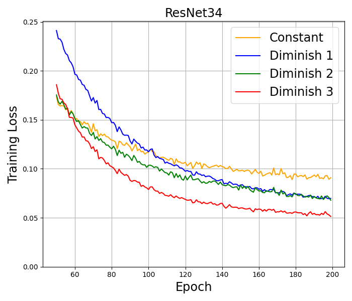
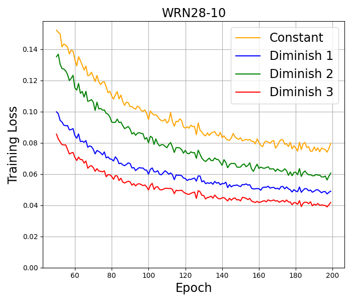
Figure 2: Training loss on CIFAR-10

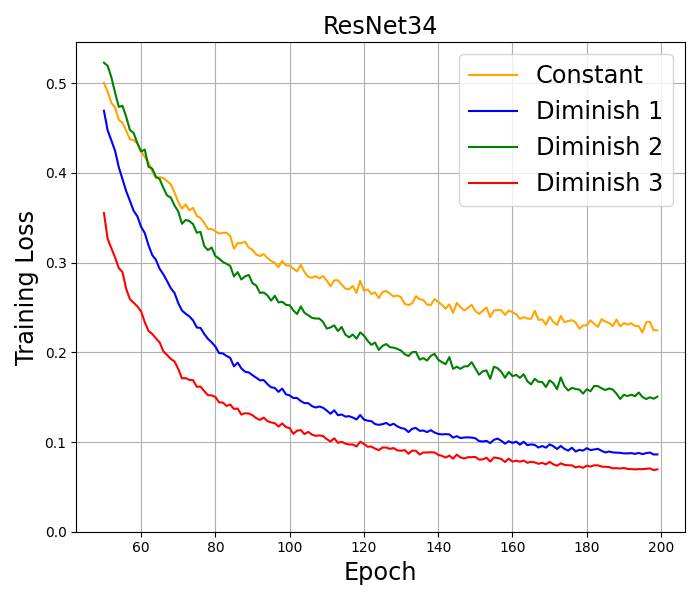
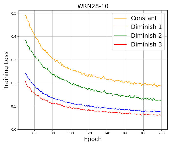
Figure 3: Training loss on CIFAR-100

The results on CIFAR-10 and CIFAR-100 indicate that SAM with Diminish 3 stepsize usually achieves the best performance in both accuracy and training loss among all tested stepsizes. In all the architectures used in the experiment, the results consistently show that diminishing stepsizes outperform constant stepsizes in terms of both accuracy and training loss measures.

6 Discussion

6.1 Conclusion

In this paper, we provide a fundamental convergence analysis of SAM and its normalized variants together with a refined convergence analysis of USAM and its unnormalized variants. Our analysis is conducted in deterministic settings under standard assumptions that cover a broad range of applications of the methods in both convex and nonconvex optimization. The conducted analysis is universal and thus can be applied in different contexts other than SAM and its variants. The performed numerical experiments show that our analysis matches the efficient implementations of SAM and its variants that are used in practice.

6.2 Limitations and Future Research

Our analysis in this paper is only conducted in deterministic settings, which leaves the stochastic and random reshuffling developments to our future research. The analysis of SAM coupling with momentum methods is also not considered in this paper and is deferred to future work. Another limitation pertains to numerical experiments, where only SAM was tested on two different datasets and three different architectures of deep learning.

Impact Statement

This paper presents work whose goal is to advance the field of Machine Learning. There are many potential societal consequences of our work, none of which are specifically highlighted here.

Appendix A Counterexamples illustrating the Insufficiency of Fundamental Convergence Properties

A.1 Example 3.1

Proof.

The iterative procedure of (7) can be written as

$$x^{k+1}=x^{k}-2t\left(x^{k}+\rho\frac{x^{k}}{|x^{k}|}\right),\text{ where }t\in[0,1/2),\;\rho>0,\;\text{ and }\;0<|x^{1}|<\frac{2t\rho}{1-2t}.$$ (14)

Then $\left\{x^{k}\right\}\not\rightarrow 0$ satisfying the inequalities

$$0<|x^{k}|<\frac{2t\rho}{1-2t}\;\text{ for all }\;k\in{\rm I\!N}.$$ (15)

It is obvious that (15) holds for $k=1.$ Assuming that this condition holds for any $k\in{\rm I\!N},$ let us show that it holds for $k+1.$ Indeed, using $x^{k}\cdot\frac{x^{k}}{|x^{k}|}>0$ and $(1-2t)|x^{k}|<2t\rho$ tells us that

$$|x^{k+1}| =\left|x^{k}-2t(x^{k}+\rho\frac{x^{k}}{|x^{k}|})\right|=\left|(1-2t)x^{k}-2t\rho\frac{x^{k}}{|x^{k}|}\right|$$

$$=\left||(1-2t)x^{k}|-|2t\rho|\right|$$

$$=2t\rho-(1-2t)|x^{k}|\in\left(0,\frac{2t\rho}{1-2t}\right),$$ (16)

and thus (15) is verified. It follows from (A.1) that $x^{k}\not\rightarrow 0.$ ∎

A.2 Example 3.4

Proof.

Observe that $x^{k}>\rho$ for all $k\in{\rm I\!N}.$ Indeed, this follows from $x^{1}>\rho$, $t_{k}<1/2$, and

$$x^{k+1}-\rho=x^{k}-\rho-2t_{k}(x^{k}-\rho)=(1-2t_{k})(x^{k}-\rho).$$

In addition, we readily get

$$0\leq x^{k+1}-\rho=(1-2t_{k})(x^{k}-\rho)=\ldots=(x^{1}-\rho)\prod_{i=1}^{k}(1-2t_{i}).$$ (17)

Furthermore, deduce from $\sum_{k=1}^{\infty}2t_{k}=\infty$ that $\prod_{k=1}^{\infty}(1-2t_{k})=0.$ Indeed, we have

$$0\leq\prod_{k=1}^{\infty}(1-2t_{k})\leq\frac{1}{\prod_{k=1}^{\infty}(1+2t_{k})}\leq\frac{1}{1+\sum_{k=1}^{\infty}2t_{k}}=0.$$

This tells us by (17) and the classical squeeze theorem that $x^{k}\rightarrow\rho$ as $k\to\infty$. ∎

Appendix B Auxiliary Results for Convergence Analysis

We first establish the new three sequences lemma, which is crucial in the analysis of both SAM, USAM, and their variants.

Lemma B.1 (three sequences lemma).

Let $\{\alpha_{k}\},\{\beta_{k}\},\{\gamma_{k}\}$ be sequences of nonnegative numbers satisfying the conditions

$$\alpha_{k+1}-\alpha_{k}\leq\beta_{k}\alpha_{k}+\gamma_{k}\;\text{ for sufficient large }\;k\in{\rm I\!N},$$ (a)

$$\left\{\beta_{k}\right\}\text{ is bounded},\sum_{k=1}^{\infty}\beta_{k}=\infty,\;\sum_{k=1}^{\infty}\gamma_{k}<\infty,\;\mbox{ and }\;\sum_{k=1}^{\infty}\beta_{k}\alpha_{k}^{2}<\infty.$$ (b)

Then we have that $\alpha_{k}\rightarrow 0$ as $k\to\infty$.

Proof.

First we show that $\liminf_{k\rightarrow\infty}\alpha_{k}=0.$ Supposing the contrary gives us some $\delta>0$ and $N\in{\rm I\!N}$ such that $\alpha_{k}\geq\delta$ for all $k\geq N$. Combining this with the second and the third condition in (b) yields

$$\infty>\sum_{k=N}^{\infty}\beta_{k}\alpha_{k}^{2}\geq\delta^{2}\sum_{k=N}^{\infty}\beta_{k}=\infty,$$

which is a contradiction verifying the claim. Let us now show that in fact $\lim_{k\rightarrow\infty}\alpha_{k}=0.$ Indeed, by the boundedness of $\left\{\beta_{k}\right\}$ define $\bar{\beta}:=\sup_{k\in{\rm I\!N}}\beta_{k}$ and deduce from (a) that there exists $K\in{\rm I\!N}$ such that

$$\alpha_{k+1}-\alpha_{k}\leq\beta_{k}\alpha_{k}+\gamma_{k}\text{ for all }k\geq K.$$ (18)

Pick $\varepsilon>0$ and find by $\liminf_{k\rightarrow\infty}\alpha_{k}=0$ and the two last conditions in (b) some $K_{\varepsilon}\in{\rm I\!N}$ with $K_{\varepsilon}\geq K$, $\alpha_{K_{\varepsilon}}\leq\varepsilon$,

$$\sum_{k=K_{\varepsilon}}^{\infty}\gamma_{k}<\frac{\varepsilon}{3},\sum_{k=K_{\varepsilon}}^{\infty}\beta_{k}\alpha_{k}^{2}<\frac{\varepsilon^{2}}{3},\;\text{ and }\;\bar{\beta}\beta_{k}\alpha_{k}^{2}\leq\frac{\varepsilon^{2}}{9}\;\text{ as }\;k\geq K_{\varepsilon}.$$ (19)

It suffices to show that $\alpha_{k}\leq 2\varepsilon$ for all $k\geq K_{\varepsilon}.$ Fix $k\geq K_{\varepsilon}$ and observe that for $\alpha_{k}\leq\varepsilon$ the desired inequality is obviously satisfied. If $\alpha_{k}>\varepsilon,$ we use $\alpha_{K_{\varepsilon}}\leq\varepsilon$ and find some $k^{\prime}<k$ such that $k^{\prime}\geq K_{\varepsilon}$ and

$$\alpha_{k^{\prime}}\leq\varepsilon\;\text{ and }\;\alpha_{i}>\varepsilon\;\text{ for }\;i=k,k-1,\ldots,k^{\prime}+1.$$

Then we deduce from (18) and (19) that

$$\alpha_{k}-\alpha_{k^{\prime}} =\sum_{i=k^{\prime}}^{k-1}\left(\alpha_{i+1}-\alpha_{i}\right)\leq\sum_{i=k^{\prime}}^{k-1}\left(\beta_{i}\alpha_{i}+\gamma_{i}\right)$$

$$=\sum_{i=k^{\prime}+1}^{k}\beta_{i}\alpha_{i}+\sum_{i=k^{\prime}}^{k-1}\gamma_{i}+\beta_{k^{\prime}}\alpha_{k^{\prime}}$$

$$\leq\frac{1}{\varepsilon}\sum_{i=k^{\prime}+1}^{k}\beta_{i}\alpha_{i}^{2}+\sum_{i=k^{\prime}}^{k-1}\gamma_{i}+\sqrt{\beta_{k^{\prime}}}\sqrt{\beta_{k^{\prime}}}\alpha_{k^{\prime}}$$

$$\leq\frac{1}{\varepsilon}\sum_{i=K_{\varepsilon}}^{\infty}\beta_{i}\alpha_{i}^{2}+\sum_{i=K_{\varepsilon}}^{\infty}\gamma_{i}+\sqrt{\bar{\beta}\beta_{k^{\prime}}\alpha_{k^{\prime}}^{2}}$$

$$\leq\frac{1}{\varepsilon}\frac{\varepsilon^{2}}{3}+\frac{\varepsilon}{3}+\frac{\varepsilon}{3}=\varepsilon.$$

As a consequence, we arrive at the estimate

$$\alpha_{k}=\alpha_{k^{\prime}}+\alpha_{k}-\alpha_{k^{\prime}}\leq\varepsilon+\varepsilon=2\varepsilon\;\mbox{ for all }\;k\geq K_{\varepsilon},$$

which verifies that $\alpha_{k}\rightarrow 0$ as $k\to\infty$ sand thus completes the proof of the lemma. ∎

Next we recall some auxiliary results from Khanh et al. (2023b).

Lemma B.2.

Let $\left\{x^{k}\right\}$ and $\left\{d^{k}\right\}$ be sequences in ${\rm I\!R}^{n}$ satisfying the condition

$$\sum_{k=1}^{\infty}\left\|x^{k+1}-x^{k}\right\|\cdot\left\|d^{k}\right\|<\infty.$$

If $\bar{x}$ is an accumulation point of the sequence $\left\{x^{k}\right\}$ and $0$ is an accumulation points of the sequence $\left\{d^{k}\right\}$, then there exists an infinite set $J\subset{\rm I\!N}$ such that we have

$$x^{k}\overset{J}{\rightarrow}\bar{x}\;\mbox{ and }\;d^{k}\overset{J}{\rightarrow}0.$$ (20)

Proposition B.3.

Let $f:{\rm I\!R}^{n}\rightarrow{\rm I\!R}$ be a $\mathcal{C}^{1}$-smooth function, and let the sequence $\left\{x^{k}\right\}\subset{\rm I\!R}^{n}$ satisfy the conditions:

• (primary descent condition). There exists $\sigma>0$ such that for sufficiently large $k\in{\rm I\!N}$ we have

  $$f(x^{k})-f(x^{k+1})\geq\sigma\left\|\nabla f(x^{k})\right\|\cdot\left\|x^{k+1}-x^{k}\right\|.$$

• (complementary descent condition). For sufficiently large $k\in{\rm I\!N}$, we have

  $$\big{[}f(x^{k+1})=f(x^{k})\big{]}\Longrightarrow[x^{k+1}=x^{k}].$$

If $\bar{x}$ is an accumulation point of $\left\{x^{k}\right\}$ and $f$ satisfies the KL property at $\bar{x}$, then $x^{k}\rightarrow\bar{x}$ as $k\to\infty$.

When the sequence under consideration is generated by a linesearch method and satisfies some conditions stronger than (H1) and (H2) in Proposition B.3, its convergence rates are established in Khanh et al. (2023b, Proposition 2.4) under the KL property with $\psi(t)=Mt^{1-q}$ as given below.

Proposition B.4.

Let $f:{\rm I\!R}^{n}\rightarrow{\rm I\!R}$ be a $\mathcal{C}^{1}$-smooth function, and let the sequences $\left\{x^{k}\right\}\subset{\rm I\!R}^{n},\left\{\tau_{k}\right\}\subset[0,\infty),\left\{d^{k}\right\}\subset{\rm I\!R}^{n}$ satisfy the iterative condition $x^{k+1}=x^{k}+\tau_{k}d^{k}$ for all $k\in{\rm I\!N}$. Assume that for all sufficiently large $k\in{\rm I\!N}$ we have $x^{k+1}\neq x^{k}$ and the estimates

$$f(x^{k})-f(x^{k+1})\geq\beta\tau_{k}\left\|d^{k}\right\|^{2}\;\text{ and }\;\left\|\nabla f(x^{k})\right\|\leq\alpha\left\|d^{k}\right\|,$$ (21)

where $\alpha,\beta>0$. Suppose in addition that the sequence $\left\{\tau_{k}\right\}$ is bounded away from $0$ $($i.e., there is some $\bar{\tau}>0$ such that $\tau_{k}\geq\bar{\tau}$ for large $k\in{\rm I\!N})$, that $\bar{x}$ is an accumulation point of $\left\{x^{k}\right\}$, and that $f$ satisfies the KL property at $\bar{x}$ with $\psi(t)=Mt^{1-q}$ for some $M>0$ and $q\in(0,1)$. Then the following convergence rates are guaranteed:

• If $q\in(0,1/2]$, then the sequence $\left\{x^{k}\right\}$ converges linearly to $\bar{x}$.

• If $q\in(1/2,1)$, then we have the estimate

  $$\left\|x^{k}-\bar{x}\right\|=\mathcal{O}\left(k^{-\frac{1-q}{2q-1}}\right).$$

Yet another auxiliary result needed below is as follows.

Proposition B.5.

Let $f:{\rm I\!R}^{n}\rightarrow{\rm I\!R}$ be a ${\cal C}^{1}$-smooth function satisfying the descent condition (5) with some constant $L>0$. Let $\left\{x^{k}\right\}$ be a sequence in ${\rm I\!R}^{n}$ that converges to $\bar{x}$, and let $\alpha>0$ be such that

$$\alpha\left\|\nabla f(x^{k})\right\|^{2}\leq f(x^{k})-f(x^{k+1})\;\text{ for sufficiently large }\;\in{\rm I\!N}.$$ (22)

Consider the following convergence rates of $\left\{x^{k}\right\}:$

• $x^{k}\rightarrow\bar{x}$ linearly.

• $\left\|x^{k}-\bar{x}\right\|=\mathcal{O}(m(k))$, where $m(k)\downarrow 0$ as $k\rightarrow\infty.$

Then (i) ensures the linear convergences of $f(x^{k})$ to $f(\bar{x})$, and $\nabla f(x^{k})$ to $0$, while (ii) yields $\left|f(x^{k})-f(\bar{x})\right|=\mathcal{O}(m^{2}(k))$ and $\left\|\nabla f(x^{k})\right\|=\mathcal{O}(m(k))$ as $k\to\infty$.

Proof.

Condition (22) tells us that there exists some $N\in{\rm I\!N}$ such that $f(x^{k+1})\leq f(x^{k})$ for all $k\geq{\rm I\!N}.$ As $x^{k}\rightarrow\bar{x}$, we deduce that $f(x^{k})\rightarrow f(\bar{x})$ with $f(x^{k})\geq f(\bar{x})$ for $k\geq N.$ Letting $k\rightarrow\infty$ in (22) and using the squeeze theorem together with the convergence of $\left\{x^{k}\right\}$ to $\bar{x}$ and the continuity of $\nabla f$ lead us to $\nabla f(\bar{x})=0.$ It follows from the descent condition of $f$ with constant $L>0$ and from (5) that

$$0\leq f(x^{k})-f(\bar{x})\leq\left\langle\nabla f(\bar{x}),x^{k}-\bar{x}\right\rangle+\dfrac{{L}}{2}\left\|x^{k}-\bar{x}\right\|^{2}=\dfrac{{L}}{2}\left\|x^{k}-\bar{x}\right\|^{2}.$$

This verifies the desired convergence rates of $\left\{f(x^{k})\right\}.$ Employing finally (22) and $f(x^{k+1})\geq f(\bar{x})$, we also get that

$$\alpha\left\|\nabla f(x^{k})\right\|^{2}\leq f(x^{k})-f(\bar{x})\text{ for all }k\geq N.$$

This immediately gives us the desired convergence rates for $\left\{\nabla f(x^{k})\right\}$ and completes the proof. ∎

Appendix C Proof of Convergence Results

C.1 Proof of Theorem 3.2

Proof.

To verify (i) first, for any $k\in{\rm I\!N}$ define $g^{k}:=\nabla f\left(x^{k}+\rho_{k}\frac{\nabla f(x^{k})}{\left\|\nabla f(x^{k})\right\|}\right)$ and get

$$\left\|g^{k}-\nabla f(x^{k})\right\| =\left\|\nabla f\left(x^{k}+\rho_{k}\frac{\nabla f(x^{k})}{\left\|\nabla f(x^{k})\right\|}\right)-\nabla f(x^{k})\right\|$$

$$\leq L\left\|x^{k}+\rho_{k}\frac{\nabla f(x^{k})}{\left\|\nabla f(x^{k})\right\|}-x^{k}\right\|=L\rho_{k}\leq L\rho,$$ (23)

where $\rho:=\sup_{k\in{\rm I\!N}}\rho_{k}.$ Using the monotonicity of $\nabla f$ due to the convexity of $f$ ensures that

$$\left\langle g^{k},\nabla f(x^{k})\right\rangle =\left\langle\nabla f\left(x^{k}+\rho_{k}\frac{\nabla f(x^{k})}{\left\|\nabla f(x^{k})\right\|}\right)-\nabla f(x^{k}),\nabla f(x^{k})\right\rangle+\left\|\nabla f(x^{k})\right\|^{2}$$

$$=\frac{\left\|\nabla f(x^{k})\right\|}{\rho_{k}}\left\langle\nabla f\left(x^{k}+\rho_{k}\frac{\nabla f(x^{k})}{\left\|\nabla f(x^{k})\right\|}\right)-\nabla f(x^{k}),\rho_{k}\frac{\nabla f(x^{k})}{\left\|\nabla f(x^{k})\right\|}\right\rangle+\left\|\nabla f(x^{k})\right\|^{2}\geq\left\|\nabla f(x^{k})\right\|^{2}.$$ (24)

With the definition of $g^{k},$ the iterative procedure (7) can also be rewritten as $x^{k+1}=x^{k}-t_{k}g^{k}$ for all $k\in{\rm I\!N}$. The first condition in (8) yields $t_{k}\downarrow 0,$ which gives us some $K\in{\rm I\!N}$ such that $Lt_{k}<1$ for all $k\geq K$. Take some such $k$. Since $\nabla f$ is Lipschitz continuous with constant $L>0$, it follows from the descent condition in (5) and the estimates in (C.1), (C.1) that

$$f(x^{k+1}) \leq f(x^{k})+\left\langle\nabla f(x^{k}),x^{k+1}-x^{k}\right\rangle+\frac{L}{2}\left\|x^{k+1}-x^{k}\right\|^{2}$$

$$=f(x^{k})-t_{k}\left\langle\nabla f(x^{k}),g^{k}\right\rangle+\frac{Lt_{k}^{2}}{2}\left\|g^{k}\right\|^{2}$$

$$=f(x^{k})-t_{k}(1-Lt_{k})\left\langle\nabla f(x^{k}),g^{k}\right\rangle+\frac{Lt_{k}^{2}}{2}\left(\left\|g^{k}-\nabla f(x^{k})\right\|^{2}-\left\|\nabla f(x^{k})\right\|^{2}\right)$$

$$\leq f(x^{k})-t_{k}(1-Lt_{k})\left\|\nabla f(x^{k})\right\|^{2}-\frac{Lt_{k}^{2}}{2}\left\|\nabla f(x^{k})\right\|^{2}+\frac{L^{3}t_{k}^{2}\rho^{2}}{2}$$

$$=f(x^{k})-\frac{t_{k}}{2}\left(2-Lt_{k}\right)\left\|\nabla f(x^{k})\right\|^{2}+\frac{L^{3}t_{k}^{2}\rho^{2}}{2}$$

$$\leq f(x^{k})-\frac{t_{k}}{2}\left\|\nabla f(x^{k})\right\|^{2}+\frac{L^{3}t_{k}^{2}\rho^{2}}{2}.$$ (25)

Rearranging the terms above gives us the estimate

$$\frac{t_{k}}{2}\left\|\nabla f(x^{k})\right\|^{2}\leq f(x^{k})-f(x^{k+1})+\frac{L^{3}t_{k}^{2}\rho^{2}}{2}.$$ (26)

Select any $M>K,$ define $S:=\frac{L^{3}\rho^{2}}{2}\sum_{k=1}^{\infty}t_{k}^{2}<\infty$, and get by taking into account $\inf_{k\in{\rm I\!N}}f(x^{k})>-\infty$ that

$$\frac{1}{2}\sum_{k=K}^{M}t_{k}\left\|\nabla f(x^{k})\right\|^{2} \leq\sum_{k=K}^{M}\left(f(x^{k})-f(x^{k+1})\right)+\sum_{k=K}^{M}\frac{L^{3}t_{k}^{2}\rho^{2}}{2}$$

$$\leq f(x^{K})-f(x^{M+1})+S$$

$$\leq f(x^{K})-\inf_{k\in{\rm I\!N}}f(x^{k})+S.$$

Letting $M\rightarrow\infty$ yields $\sum_{k=K}^{\infty}t_{k}\left\|\nabla f(x^{k})\right\|^{2}<\infty.$ Let us now show that $\liminf\left\|\nabla f(x^{k})\right\|=0.$ Supposing the contrary gives us $\varepsilon>0$ and $N\geq K$ such that $\left\|\nabla f(x^{k})\right\|\geq\varepsilon$ for all $k\geq N$, which tells us that

$$\infty>\sum_{k=N}^{\infty}t_{k}\left\|\nabla f(x^{k})\right\|^{2}\geq\varepsilon^{2}\sum_{k=N}^{\infty}t_{k}=\infty.$$

This clearly contradicts the second condition in (8) and this justifies (i).

To verify (ii), define $u_{k}:=\frac{L^{3}\rho^{2}}{2}\sum_{i=k}^{\infty}t_{i}^{2}\;\text{ for all }\;k\in{\rm I\!N}$ and deduce from the first condition in (8) that $u_{k}\downarrow 0$ as $k\rightarrow\infty.$ With the usage of $\left\{u_{k}\right\},$ estimate (26) is written as

$$f(x^{k+1})+u_{k+1}\leq f(x^{k})+u_{k}-\frac{t_{k}}{2}\left\|\nabla f(x^{k})\right\|^{2}\;\text{ for all }\;k\geq K,$$

which means that $\left\{f(x^{k})+u_{k}\right\}_{k\geq K}$ is nonincreasing. It follows from $\inf_{k\in{\rm I\!N}}f(x^{k})>-\infty$ and $u_{k}\downarrow 0$ that $\left\{f(x^{k})+u_{k}\right\}$ is convergent, which means that the sequence $\left\{f(x^{k})\right\}$ is convergent as well. Assume now $f$ has some nonempty and bounded level set. Then every level set of $f$ is bounded by Ruszczynski (2006, Exercise 2.12). By (26), we get that

$$f(x^{k+1})\leq f(x^{k})+\frac{L^{3}\rho^{2}}{2}t_{k}^{2}-\frac{t_{k}}{2}\left\|\nabla f(x^{k})\right\|^{2}\leq f(x^{k})+\frac{L^{3}\rho^{2}}{2}t_{k}^{2}\;\text{ for all }\;k\geq K.$$

Proceeding by induction leads us to

$$f(x^{k+1})\leq f(x^{1})+\frac{L^{3}\rho^{2}}{2}\sum_{i=1}^{k}t_{i}^{2}\leq f(x^{1})+S\;\text{ for all }\;k\geq K,$$

which means that $x^{k+1}\in\left\{x\in{\rm I\!R}^{n}\;|\;f(x)\leq f(x^{1})+S\right\}$ for all $k\geq K$ and thus justifies the boundedness of $\left\{x^{k}\right\}$.

Taking $\liminf\left\|\nabla f(x^{k})\right\|=0$ into account gives us an infinite set $J\subset{\rm I\!N}$ such that $\left\|\nabla f(x^{k})\right\|\overset{J}{\rightarrow}0.$ As $\left\{x^{k}\right\}$ is bounded, the sequence $\left\{x^{k}\right\}_{k\in J}$ is also bounded, which gives us another infinite set $I\subset J$ and $\bar{x}\in{\rm I\!R}^{n}$ such that $x^{k}\overset{I}{\rightarrow}\bar{x}.$ By

$$\lim_{k\in I}\left\|\nabla f(x^{k})\right\|=\lim_{k\in J}\left\|\nabla f(x^{k})\right\|=0$$

and the continuity of $\nabla f$, we get that $\nabla f(\bar{x})=0$ ensuring that $\bar{x}$ is a global minimizer of $f$ with the optimal value $f^{*}:=f(\bar{x}).$ Since the sequence $\left\{f(x^{k})\right\}$ is convergent and since $\bar{x}$ is an accumulation point of $\left\{x^{k}\right\}$, we conclude that $f^{*}=f(\bar{x})$ is the limit of $\left\{f(x^{k})\right\}$. Now take any accumulation point $\widetilde{x}$ of $\left\{x^{k}\right\}$ and find an infinite set $J^{\prime}\subset{\rm I\!N}$ with $x^{k}\overset{J^{\prime}}{\rightarrow}\widetilde{x}.$ As $\left\{f(x^{k})\right\}$ converges to $f^{*}$, we deduce that

$$f(\widetilde{x})=\lim_{k\in J^{\prime}}f(x^{k})=\lim_{k\in{\rm I\!N}}f(x^{k})=f^{*},$$

which implies that $\widetilde{x}$ is also a global minimizer of $f.$ Assuming in addition that $f$ has a unique minimizer $\bar{x}$ and taking any accumulation point $\widetilde{x}$ of $\left\{x^{k}\right\},$ we get that $\widetilde{x}$ is a minimizer of $f,$ i.e., $\widetilde{x}=\bar{x}.$ This means that $\bar{x}$ is the unique accumulation point of $\left\{x^{k}\right\}$, and therefore $x^{k}\rightarrow\bar{x}$ as $k\to\infty$. ∎

C.2 Proof of Theorem 3.3

Proof.

By (9), we find some $c_{1}>0,c_{2}\in(0,1)$, and $K\in{\rm I\!N}$ such that

$$\frac{1}{2}(2-Lt_{k}-\varepsilon_{k}+Lt_{k}\varepsilon_{k})\geq c_{1},\quad\frac{1}{2}(1-Lt_{k})+\frac{Lt_{k}\varepsilon_{k}}{2}\leq c_{2},\;\mbox{ and}\quad Lt_{k}<1\;\text{ for all }\;k\geq K.$$ (27)

Let us first verify the estimate

$$f(x^{k+1})\leq f(x^{k})-c_{1}t_{k}\left\|\nabla f(x^{k})\right\|^{2}+c_{2}t_{k}\varepsilon_{k}\;\text{ whenever }\;k\geq K.$$ (28)

To proceed, fix $k\in{\rm I\!N}$ and deduce from the Cauchy-Schwarz inequality that

$$\left\langle g^{k},\nabla f(x^{k})\right\rangle =\left\langle g^{k}-\nabla f(x^{k}),\nabla f(x^{k})\right\rangle+\left\|\nabla f(x^{k})\right\|^{2}$$

$$\geq-\left\|g^{k}-\nabla f(x^{k})\right\|\cdot\left\|\nabla f(x^{k})\right\|+\left\|\nabla f(x^{k})\right\|^{2}$$

$$\geq-\varepsilon_{k}\left\|\nabla f(x^{k})\right\|+\left\|\nabla f(x^{k})\right\|^{2}.$$ (29)

Since $\nabla f$ is Lipschitz continuous with constant $L$, it follows from the descent condition in (5) and the estimate (C.2) that

$$f(x^{k+1}) \leq f(x^{k})+\left\langle\nabla f(x^{k}),x^{k+1}-x^{k}\right\rangle+\frac{L}{2}\left\|x^{k+1}-x^{k}\right\|^{2}$$

$$=f(x^{k})-t_{k}\left\langle\nabla f(x^{k}),g^{k}\right\rangle+\frac{Lt_{k}^{2}}{2}\left\|g^{k}\right\|^{2}$$

$$=f(x^{k})-t_{k}(1-Lt_{k})\left\langle\nabla f(x^{k}),g^{k}\right\rangle+\frac{Lt_{k}^{2}}{2}(\left\|g^{k}-\nabla f(x^{k})\right\|^{2}-\left\|\nabla f(x^{k})\right\|^{2})$$

$$\leq f(x^{k})-t_{k}(1-Lt_{k})\left(-\varepsilon_{k}\left\|\nabla f(x^{k})\right\|+\left\|\nabla f(x^{k})\right\|^{2}\right)+\frac{Lt_{k}^{2}\varepsilon_{k}^{2}}{2}-\frac{Lt_{k}^{2}}{2}\left\|\nabla f(x^{k})\right\|^{2}$$

$$=f(x^{k})-\frac{t_{k}}{2}(2-{Lt_{k}})\left\|\nabla f(x^{k})\right\|^{2}+t_{k}(1-Lt_{k})\varepsilon_{k}\left\|\nabla f(x^{k})\right\|+\frac{Lt_{k}^{2}\varepsilon_{k}^{2}}{2}$$

$$\leq f(x^{k})-\frac{t_{k}}{2}(2-{Lt_{k}})\left\|\nabla f(x^{k})\right\|^{2}+\frac{1}{2}t_{k}(1-Lt_{k})\varepsilon_{k}\left(1+\left\|\nabla f(x^{k})\right\|^{2}\right)+\frac{Lt_{k}^{2}\varepsilon_{k}^{2}}{2}$$

$$=f(x^{k})-\frac{t_{k}}{2}(2-Lt_{k}-\varepsilon_{k}+Lt_{k}\varepsilon_{k})\left\|\nabla f(x^{k})\right\|^{2}+\frac{1}{2}t_{k}\varepsilon_{k}(1-Lt_{k})+\frac{Lt_{k}^{2}\varepsilon_{k}^{2}}{2}$$

$$=f(x^{k})-\frac{t_{k}}{2}(2-Lt_{k}-\varepsilon_{k}+Lt_{k}\varepsilon_{k})\left\|\nabla f(x^{k})\right\|^{2}+t_{k}\varepsilon_{k}\left(\frac{1}{2}(1-Lt_{k})+\frac{Lt_{k}\varepsilon_{k}}{2}.\right)$$

Combining this with (27) gives us (28). Defining $u_{k}:=c_{2}\sum_{i=k}^{\infty}t_{i}\varepsilon_{i}$ for $k\in{\rm I\!N}$, we get that $u_{k}\rightarrow 0$ as $k\rightarrow\infty$ and $u_{k}-u_{k+1}=t_{k}\varepsilon_{k}$ for all $k\in{\rm I\!N}.$ Then (28) can be rewritten as

$$f(x^{k+1})+u_{k+1}\leq f(x^{k})+u_{k}-c_{1}t_{k}\left\|\nabla f(x^{k})\right\|^{2},\quad k\geq K.$$ (30)

To proceed now with the proof of (i), we deduce from (30) combined with $\inf f(x^{k})>-\infty$ and $u_{k}\rightarrow 0$ as $k\rightarrow\infty$ that

$$c_{1}\sum_{k=K}^{\infty}t_{k}\left\|\nabla f(x^{k})\right\|^{2} \leq\sum_{k=K}^{\infty}(f(x^{k})-f(x^{k+1})+u_{k}-u_{k+1})$$

$$\leq f(x^{K})-\inf_{k\in{\rm I\!N}}f(x^{k})+u_{K}<\infty.$$

Next we employ Lemma B.1 with $\alpha_{k}:=\left\|\nabla f(x^{k})\right\|$, $\beta_{k}:=Lt_{k}$, and $\gamma_{k}:=Lt_{k}\varepsilon_{k}$ for all $k\in{\rm I\!N}$ to derive $\nabla f(x^{k})\rightarrow 0.$ Observe first that condition (a) is satisfied due to the the estimates

$${\alpha_{k+1}-\alpha_{k}} ={\left\|\nabla f(x^{k+1})\right\|-\left\|\nabla f(x^{k})\right\|}\leq\left\|\nabla f(x^{k+1})-\nabla f(x^{k})\right\|$$

$$\leq L\left\|x^{k+1}-x^{k}\right\|=Lt_{k}\left\|g^{k}\right\|$$

$$\leq Lt_{k}(\left\|\nabla f(x^{k})\right\|+\left\|g^{k}-\nabla f(x^{k})\right\|)$$

$$\leq Lt_{k}(\left\|\nabla f(x^{k})\right\|+\varepsilon_{k})$$

$$=\beta_{k}\alpha_{k}+\gamma_{k}\;\text{ for all }\;k\in{\rm I\!N}.$$

Further, the conditions in (b) hold by (9) and $\sum_{k=1}^{\infty}t_{k}\left\|\nabla f(x^{k})\right\|^{2}<\infty.$ As all the assumptions (a), (b) are satisfied, Lemma B.1 tells us that $\left\|\nabla f(x^{k})\right\|=\alpha_{k}\rightarrow 0$ as $k\rightarrow\infty.$

To verify (ii), deduce from (30) that $\left\{f(x^{k})+u_{k}\right\}$ is nonincreasing. As $\inf_{k\in{\rm I\!N}}f(x^{k})>-\infty$ and $u_{k}\rightarrow 0,$ we get that $\left\{f(x^{k})+u_{k}\right\}$ is bounded from below, and thus is convergent. Taking into account that $u_{k}\rightarrow 0$, it follows that $f(x^{k})$ is convergent as well. Since $\bar{x}$ is an accumulation point of $\left\{x^{k}\right\},$ the continuity of $f$ tells us that $f(\bar{x})$ is also an accumulation point of $\left\{f(x^{k})\right\},$ which immediately yields $f(x^{k})\rightarrow f(\bar{x})$ due to the convergence of $\left\{f(x^{k})\right\}.$

It remains to verify (iii). By the KL property of $f$ at $\bar{x},$ we find some $\eta>0,$ a neighborhood $U$ of $\bar{x}$, and a desingularizing concave continuous function $\varphi:[0,\eta)\rightarrow[0,\infty)$ such that $\varphi(0)=0$, $\varphi$ is $\mathcal{C}^{1}$-smooth on $(0,\eta)$, $\varphi^{\prime}>0$ on $(0,\eta)$, and we have for all $x\in U$ with $0<f(x)-f(\bar{x})<\eta$ that

$$\varphi^{\prime}(f(x)-f(\bar{x}))\left\|\nabla f(x)\right\|\geq 1.$$ (31)

Let $\bar{K}>K$ be natural number such that $f(x^{k})>f(\bar{x})$ for all $k\geq\bar{K}$. Define $\Delta_{k}:=\varphi(f(x^{k})-f(\bar{x})+u_{k})$ for all $k\geq\bar{K}$, and let $R>0$ be such that $\mathbb{B}(\bar{x},R)\subset U$. Taking the number $C$ from Assumption 2.3, remembering that $\bar{x}$ is an accumulation point of $\left\{x^{k}\right\},$ and using $f(x^{k})+u_{k}\downarrow f(\bar{x})$, $\Delta_{k}\downarrow 0$ as $k\rightarrow\infty$ together with condition (10), we get by choosing a larger $\bar{K}$ that $f(x^{\bar{K}})+u_{\bar{K}}<f(\bar{x})+\eta$ and

$$\left\|x^{\bar{K}}-\bar{x}\right\|+\frac{1}{{Cc_{1}}}\Delta_{\bar{K}}+\sum_{k={\bar{K}}}^{\infty}t_{k}\varphi^{\prime}\left(\sum_{i=k}^{\infty}t_{i}\varepsilon_{i}\right)^{-1}+\sum_{k=\bar{K}}^{\infty}t_{k}\varepsilon_{k}<R.$$ (32)

Let us now show by induction that $x^{k}\in\mathbb{B}(\bar{x},R)$ for all $k\geq\bar{K}.$ The assertion obviously holds for $k=\bar{K}$ due to (32). Take some $\widehat{K}\geq\bar{K}$ and suppose that $x^{k}\in U$ for all $k=\bar{K},\ldots,\widehat{K}.$ We intend to show that $x^{\widehat{K}+1}\in\mathbb{B}(\bar{x},R)$ as well. To proceed, fix some $k\in\left\{\bar{K},\ldots,\widehat{K}\right\}$ and get by $f(\bar{x})<f(x^{k})<f(x^{k})+u_{k}<f(\bar{x})+\eta$ that

$$\varphi^{\prime}(f(x^{k})-f(\bar{x}))\left\|\nabla f(x^{k})\right\|\geq 1.$$ (33)

Combining this with $u_{k}>0$ and $f(x^{k})-f(\bar{x})>0$ gives us

$$\Delta_{k}-\Delta_{k+1} \geq\varphi^{\prime}(f(x^{k})-f(\bar{x})+u_{k})(f(x^{k})+u_{k}-f(x^{k+1})-u_{k+1})$$ (34a)

$$\geq\varphi^{\prime}(f(x^{k})-f(\bar{x})+u_{k})c_{1}t_{k}\left\|\nabla f(x^{k})\right\|^{2}$$ (34b)

$$\geq\frac{C}{\left(\varphi^{\prime}(f(x^{k})-f(\bar{x}))\right)^{-1}+\left(\varphi^{\prime}(u_{k})\right)^{-1}}c_{1}t_{k}\left\|\nabla f(x^{k})\right\|^{2}$$ (34c)

$$\geq\frac{C}{\left\|\nabla f(x^{k})\right\|+\left(\varphi^{\prime}(u_{k})\right)^{-1}}c_{1}t_{k}\left\|\nabla f(x^{k})\right\|^{2},$$ (34d)

where (34a) follows from the concavity of $\varphi$, (34b) follows from (30), (34c) follows from Assumption 2.3, and (34d) follows from (33). Taking the square root of both sides in (34d) and employing the AM-GM inequality yield

$$t_{k}\left\|\nabla f(x^{k})\right\|=\sqrt{t_{k}}\cdot\sqrt{t_{k}\left\|\nabla f(x^{k})\right\|^{2}} \leq\sqrt{\frac{1}{Cc_{1}}(\Delta_{k}-\Delta_{k+1})t_{k}(\left\|\nabla f(x^{k})\right\|+\left(\varphi^{\prime}(u_{k})\right)^{-1}})$$

$$\leq\frac{1}{2Cc_{1}}(\Delta_{k}-\Delta_{k+1})+\frac{1}{2}t_{k}\left(\left(\varphi^{\prime}(u_{k})\right)^{-1}+\left\|\nabla f(x^{k})\right\|\right).$$ (35)

Using the nonincreasing property of $\varphi^{\prime}$ due to the concavity of $\varphi$ and the choice of $c_{2}\in(0,1)$ ensures that

$$\left(\varphi^{\prime}(u_{k})\right)^{-1}=\left(\varphi^{\prime}(c_{2}\sum_{i=k}^{\infty}t_{i}\varepsilon_{i})\right)^{-1}\leq\left(\varphi^{\prime}(\sum_{i=k}^{\infty}t_{i}\varepsilon_{i})\right)^{-1}.$$

Rearranging terms and taking the sum over $k=\bar{K},\ldots,\widehat{K}$ of inequality (C.2) gives us

$$\sum_{k={\bar{K}}}^{\widehat{K}}t_{k}\left\|\nabla f(x^{k})\right\| \leq\frac{1}{{Cc_{1}}}\sum_{k={\bar{K}}}^{\widehat{K}}(\Delta_{k}-\Delta_{k+1})+\sum_{k={\bar{K}}}^{\widehat{K}}t_{k}\varphi^{\prime}(u_{k})^{-1}$$

$$=\frac{1}{{Cc_{1}}}(\Delta_{\bar{K}}-\Delta_{\widehat{K}})+\sum_{k={\bar{K}}}^{\widehat{K}}t_{k}\varphi^{\prime}\left(c_{2}\sum_{i=k}^{\infty}t_{i}\varepsilon_{i}\right)^{-1}$$

$$\leq\frac{1}{{Cc_{1}}}\Delta_{\bar{K}}+\sum_{k=\bar{K}}^{\widehat{K}}t_{k}\varphi^{\prime}\left(\sum_{i=k}^{\infty}t_{i}\varepsilon_{i}\right)^{-1}.$$

The latter estimate together with the triangle inequality and (32) tells us that

$$\left\|x^{\widehat{K}+1}-\bar{x}\right\| =\left\|x^{\bar{K}}-\bar{x}\right\|+\sum_{k={\bar{K}}}^{\widehat{K}}\left\|x^{k+1}-x^{k}\right\|$$

$$=\left\|x^{\bar{K}}-\bar{x}\right\|+\sum_{k={\bar{K}}}^{\widehat{K}}t_{k}\left\|g^{k}\right\|$$

$$\leq\left\|x^{\bar{K}}-\bar{x}\right\|+\sum_{k={\bar{K}}}^{\widehat{K}}t_{k}\left\|\nabla f(x^{k})\right\|+\sum_{k={\bar{K}}}^{\widehat{K}}t_{k}\left\|g^{k}-\nabla f(x^{k})\right\|$$

$$\leq\left\|x^{\bar{K}}-\bar{x}\right\|+\sum_{k={\bar{K}}}^{\widehat{K}}t_{k}\left\|\nabla f(x^{k})\right\|+\sum_{k={\bar{K}}}^{\widehat{K}}t_{k}\varepsilon_{k}$$

$$\leq\left\|x^{\bar{K}}-\bar{x}\right\|+\frac{1}{Cc_{1}}\Delta_{\bar{K}}+\sum_{k={\bar{K}}}^{\infty}t_{k}\varphi^{\prime}\left(\sum_{i=k}^{\infty}t_{i}\varepsilon_{i}\right)^{-1}+\sum_{k={\bar{K}}}^{\infty}t_{k}\varepsilon_{k}<R.$$

By induction, this means that $x^{k}\in\mathbb{B}(\bar{x},R)$ for all $k\geq{\bar{K}}.$ Then a similar device brings us to

$$\sum_{k=\bar{K}}^{\widehat{K}}t_{k}\left\|\nabla f(x^{k})\right\|\leq\frac{1}{{Cc_{1}}}\Delta_{\bar{K}}+\sum_{k={\bar{K}}}^{\infty}t_{k}\varphi^{\prime}\left(\sum_{i=k}^{\infty}t_{i}\varepsilon_{i}\right)^{-1}\text{ for all }\widehat{K}\geq\bar{K},$$

which yields $\sum_{k=1}^{\infty}t_{k}\left\|\nabla f(x^{k})\right\|<\infty$. Therefore,

$$\sum_{k=1}^{\infty}\left\|x^{k+1}-x^{k}\right\| =\sum_{k=1}^{\infty}t_{k}\left\|g^{k}\right\|\leq\sum_{k=1}^{\infty}t_{k}\left\|\nabla f(x^{k})\right\|+\sum_{k=1}^{\infty}t_{k}\left\|g^{k}-\nabla f(x^{k})\right\|$$

$$\leq\sum_{k=1}^{\infty}t_{k}\left\|\nabla f(x^{k})\right\|+\sum_{k=1}^{\infty}t_{k}\varepsilon_{k}<\infty$$

which justifies the convergence of $\left\{x^{k}\right\}$ and thus completes the proof of the theorem. ∎

C.3 Proof of Theorem 4.1

Proof.

Using $\left\|\nabla f(x^{k})-g^{k}\right\|\leq\nu\left\|\nabla f(x^{k})\right\|$ gives us the estimates

$$\left\|g^{k}\right\|^{2} =\left\|\nabla f(x^{k})-g^{k}\right\|^{2}-\left\|\nabla f(x^{k})\right\|^{2}+2\left\langle\nabla f(x^{k}),g^{k}\right\rangle$$

$$\leq\nu^{2}\left\|\nabla f(x^{k})\right\|^{2}-\left\|\nabla f(x^{k})\right\|^{2}+2\left\langle\nabla f(x^{k}),g^{k}\right\rangle$$

$$=-(1-\nu^{2})\left\|\nabla f(x^{k})\right\|^{2}+2\left\langle\nabla f(x^{k}),g^{k}\right\rangle,$$ (36)

$$\left\langle\nabla f(x^{k}),g^{k}\right\rangle =\left\langle\nabla f(x^{k}),g^{k}-\nabla f(x^{k})\right\rangle+\left\|\nabla f(x^{k})\right\|^{2}$$

$$\leq\left\|\nabla f(x^{k})\right\|\cdot\left\|g^{k}-\nabla f(x^{k})\right\|+\left\|\nabla f(x^{k})\right\|^{2}$$

$$\leq(1+\nu)\left\|\nabla f(x^{k})\right\|^{2},$$ (37)

$$-\left\langle\nabla f(x^{k}),g^{k}\right\rangle =-\left\langle\nabla f(x^{k}),g^{k}-\nabla f(x^{k})\right\rangle-\left\|\nabla f(x^{k})\right\|^{2}$$

$$\leq\left\|\nabla f(x^{k})\right\|\cdot\left\|g^{k}-\nabla f(x^{k})\right\|-\left\|\nabla f(x^{k})\right\|^{2}$$

$$\leq-(1-\nu)\left\|\nabla f(x^{k})\right\|^{2},$$ (38)

$$\left\|\nabla f(x^{k})\right\|-\left\|g^{k}-\nabla f(x^{k})\right\| \leq\left\|g^{k}\right\|\leq\left\|\nabla f(x^{k})\right\|+\left\|g^{k}-\nabla f(x^{k})\right\|,$$

which in turn imply that

$$(1-\nu)\left\|\nabla f(x^{k})\right\|\leq\left\|g^{k}\right\|\leq(1+\nu)\left\|\nabla f(x^{k})\right\|\text{ for all }k\in{\rm I\!N}.$$ (39)

Using condition (13), we find $N\in{\rm I\!N}$ so that $2-2\nu-Lt_{k}(1+\nu)^{2}\geq\delta$ for all $k\geq N.$ Select such a natural number $k$ and use the Lipschitz continuity of $\nabla f$ with constant $L$ to deduce from the descent condition (5), the relationship $x^{k+1}=x^{k}-t_{k}g^{k}$, and the estimates (36)–(38) that

$$f(x^{k+1}) \leq f(x^{k})+\left\langle\nabla f(x^{k}),x^{k+1}-x^{k}\right\rangle+\dfrac{L}{2}\left\|x^{k+1}-x^{k}\right\|^{2}$$

$$=f(x^{k})-t_{k}\left\langle\nabla f(x^{k}),g^{k}\right\rangle+\dfrac{Lt_{k}^{2}}{2}\left\|g^{k}\right\|^{2}$$

$$\leq f(x^{k})-t_{k}\left\langle\nabla f(x^{k}),g^{k}\right\rangle+Lt_{k}^{2}\left\langle\nabla f(x^{k}),g^{k}\right\rangle-\frac{Lt_{k}^{2}(1-\nu^{2})}{2}\left\|\nabla f(x^{k})\right\|^{2}$$

$$\leq f(x^{k})-t_{k}(1-\nu)\left\|\nabla f(x^{k})\right\|^{2}+Lt_{k}^{2}(1+\nu)\left\|\nabla f(x^{k})\right\|^{2}-\frac{Lt_{k}^{2}(1-\nu^{2})}{2}\left\|\nabla f(x^{k})\right\|^{2}$$

$$=f(x^{k})-\frac{t_{k}}{2}\left(2-2\nu-Lt_{k}(1+\nu)^{2}\right)\left\|\nabla f(x^{k})\right\|^{2}$$

$$\leq f(x^{k})-\frac{\delta t_{k}}{2}\left\|\nabla f(x^{k})\right\|^{2}\text{ for all }k\geq N.$$ (40)

It follows from the above that the sequence $\left\{f(x^{k})\right\}_{k\geq N}$ is nonincreasing, and hence the condition $\inf_{k\in{\rm I\!N}}f(x^{k})>-\infty$ ensures the convergence of $\left\{f(x^{k})\right\}$. This allows us to deduce from (40) that

$$\frac{\delta}{2}\sum_{k=N}^{\infty}t_{k}\left\|\nabla f(x^{k})\right\|^{2}\leq\sum_{K=N}^{\infty}(f(x^{k})-f(x^{k+1}))\leq f(x^{K})-\inf_{k\in{\rm I\!N}}f(x^{k})<\infty.$$ (41)

Combining the latter with (39) and $x^{k+1}=x^{k}-t_{k}g^{k}$ gives us

$$\sum_{k=1}^{\infty}\left\|x^{k+1}-x^{k}\right\|\cdot\left\|g^{k}\right\|=\sum_{k=1}^{\infty}t_{k}\left\|g^{k}\right\|^{2}\leq(1+\nu)^{2}\sum_{k=1}^{\infty}t_{k}\left\|\nabla f(x^{k})\right\|^{2}<\infty.$$ (42)

Now we are ready to verify all the assertions of the theorem. Let us start with (i) and show that $0$ in an accumulation point of $\left\{g^{k}\right\}$. Indeed, supposing the contrary gives us $\varepsilon>0$ and $K\in{\rm I\!N}$ such that $\left\|g^{k}\right\|\geq\varepsilon$ for all $k\geq K$, and therefore

$$\infty>\sum_{k=K}^{\infty}t_{k}\left\|g^{k}\right\|^{2}\geq\sum_{k=K}^{\infty}t_{k}=\infty,$$

which is a contradiction justifying that $0$ is an accumulation point of $\left\{g^{k}\right\}$. If $\bar{x}$ is an accumulation point of $\left\{x^{k}\right\},$ then by Lemma B.2 and (42), we find an infinite set $J\subset N$ such that $x^{k}\overset{J}{\rightarrow}\bar{x}$ and $g^{k}\overset{J}{\rightarrow}0.$ The latter being combined with (39) gives us $\nabla f(x^{k})\overset{J}{\rightarrow}0$, which yields the stationary condition $\nabla f(\bar{x})=0.$

To verity (ii), let $\bar{x}$ be an accumulation point of $\left\{x^{k}\right\}$ and find an infinite set $J\subset{\rm I\!N}$ such that $x^{k}\overset{J}{\rightarrow}\bar{x}.$ Combining this with the continuity of $f$ and the fact that $\left\{f(x^{k})\right\}$ is convergent, we arrive at the equalities

$$f(\bar{x})=\lim_{k\in J}f(x^{k})=\lim_{k\in{\rm I\!N}}f(x^{k}),$$

which therefore justify assertion (ii).

To proceed with the proof of the next assertion (iii), assume that $\nabla f$ is Lipschitz continuous with constant $L>0$ and employ Lemma B.1 with $\alpha_{k}:=\left\|\nabla f(x^{k})\right\|$, $\beta_{k}:=Lt_{k}(1+\nu)$, and $\gamma_{k}:=0$ for all $k\in{\rm I\!N}$ to derive that $\nabla f(x^{k})\rightarrow 0.$ Observe first that condition (a) of this lemma is satisfied due to the the estimates

$$\alpha_{k+1}-\alpha_{k} =\left\|\nabla f(x^{k+1})\right\|-\left\|\nabla f(x^{k})\right\|$$

$$\leq\left\|\nabla f(x^{k+1})-\nabla f(x^{k})\right\|\leq L\left\|x^{k+1}-x^{k}\right\|$$

$$=Lt_{k}\left\|g^{k}\right\|\leq Lt_{k}(1+\nu)\left\|\nabla f(x^{k})\right\|=\beta_{k}\alpha_{k}.$$

The conditions in (b) of the lemma are satisfied since $\left\{t_{k}\right\}$ is bounded, $\sum_{k=1}^{\infty}t_{k}=\infty$ by (13), $\gamma_{k}=0$, and

$$\sum_{k=1}^{\infty}\beta_{k}\alpha_{k}^{2}=L(1+\nu)\sum_{k=1}^{\infty}t_{k}\left\|\nabla f(x^{k})\right\|^{2}<\infty,$$

where the inequality follows from (41). Thus applying Lemma B.1 gives us $\nabla f(x^{k})\rightarrow 0$ as $k\to\infty$.

To prove (iv), we verify the assumptions of Proposition B.3 for the sequences generated by Algorithm 2. It follows from (40) and $x^{k+1}=x^{k}-t_{k}g^{k}$ that

$$f(x^{k+1}) \leq f(x^{k})-\frac{\delta t_{k}}{2(1+\nu)}\left\|\nabla f(x^{k})\right\|\cdot\left\|g^{k}\right\|$$

$$=f(x^{k})-\frac{\delta}{2(1+\nu)}\left\|\nabla f(x^{k})\right\|\cdot\left\|x^{k+1}-x^{k}\right\|,$$ (43)

which justify (H1) with $\sigma=\frac{\delta}{2(1+\nu)}$. Regarding condition (H2), assume that $f(x^{k+1})=f(x^{k})$ and get by (40) that $\nabla f(x^{k})=0$, which implies by $\left\|g^{k}-\nabla f(x^{k})\right\|\leq\nu\left\|\nabla f(x^{k})\right\|$ that $g^{k}=0.$ Combining this with $x^{k+1}=x^{k}-t_{k}g^{k}$ gives us $x^{k+1}=x^{k},$ which verifies (H2). Therefore, Proposition B.3 tells us that $\left\{x^{k}\right\}$ is convergent.

Let us now verify the final assertion (v) of the theorem. It is nothing to prove if $\left\{x^{k}\right\}$ stops at a stationary point after a finite number of iterations. Thus we assume that $\nabla f(x^{k})\neq 0$ for all $k\in{\rm I\!N}.$ The assumptions in (v) give us $\bar{t}>0$ and $N\in{\rm I\!N}$ such that $t_{k}\geq\bar{t}$ for all $k\geq N.$ Let us check that the assumptions of Proposition B.4 hold for the sequences generated by Algorithm 2 with $\tau_{k}:=t_{k}$ and $d^{k}:=-g^{k}$ for all $k\in{\rm I\!N}$. The iterative procedure $x^{k+1}=x^{k}-t_{k}g^{k}$ can be rewritten as $x^{k+1}=x^{k}+t_{k}d^{k}$. Using the first condition in (39) and taking into account that $\nabla f(x^{k})\neq 0$ for all $k\in{\rm I\!N},$ we get that $g^{k}\neq 0$ for all $k\in{\rm I\!N}.$ Combining this with $x^{k+1}=x^{k}-t_{k}g^{k}$ and $t_{k}\geq\bar{t}$ for all $k\geq N,$ tells us that $x^{k+1}\neq x^{k}$ for all $k\geq N.$ It follows from (40) and (39) that

$$f(x^{k+1}) \leq f(x^{k})-\frac{\delta t_{k}}{2(1+\nu)^{2}}\left\|g^{k}\right\|^{2}.$$ (44)

This estimate together with the second inequality in (39) verifies (21) with $\beta=\frac{\delta}{2(1+\nu)^{2}},\alpha=\frac{1}{1-\nu}$. As all the assumptions are verified, Proposition B.4 gives us the assertions:

• If $q\in(0,1/2]$, then the sequence $\left\{x^{k}\right\}$ converges linearly to $\bar{x}$.

• If $q\in(1/2,1)$, then we have the estimate

  $$\left\|x^{k}-\bar{x}\right\|=\mathcal{O}\left(k^{-\frac{1-q}{2q-1}}\right).$$

The convergence rates of $\left\{f(x^{k})\right\}$ and $\left\{\left\|\nabla f(x^{k})\right\|\right\}$ follow now from Proposition B.5, and thus we are done. ∎

Appendix D Additional Remarks

Remark D.1.

Assumption 2.3 is satisfied with constant $C=1$ for $\varphi(t)=Mt^{1-q}$ with $M>0$ and $q\in[0,1)$. Indeed, taking any $x,y>0$ with $x+y<\eta$, we deduce that $(x+y)^{q}\leq x^{q}+y^{q},$ and hence

$$[\varphi^{\prime}(x+y)]^{-1} =\frac{1}{M(1-q)}(x+y)^{q}\leq\frac{1}{M(1-q)}(x^{q}+y^{q})=(\varphi^{\prime}(x))^{-1}+(\varphi^{\prime}(y))^{-1}.$$

Remark D.2.

Construct an example to demonstrate that the conditions in (12) do not require that ${\rho_{k}}$ converges to $0$. Let $L>0$ be a Lipschitz constant of $\nabla f$, let $C$ be a positive constant such that $C<2/L$, let $P\subset{\rm I\!N}$ be the set of all perfect squares, let $t_{k}=\frac{1}{k}$ for all $k\in{\rm I\!N},p>0$, and let $\left\{\rho_{k}\right\}$ be constructed as follows:

$$\rho_{k}=\begin{cases}C,&k\in P,\\ \frac{C}{k^{p}},&k\notin P,\end{cases}\;\text{ which yields }\;{t_{k}}{\rho_{k}}=\begin{cases}\frac{C}{k},&k\in P,\\ \frac{C}{k^{p+1}},&k\notin P.\end{cases}$$

It is clear from the construction of $\left\{\rho_{k}\right\}$ that $\limsup_{k\rightarrow\infty}\rho_{k}=C>0$, which implies that $\left\{\rho_{k}\right\}$ does not convergence to $0.$ We also immediately deduce that $\sum_{k=1}^{\infty}t_{k}=\infty,\;t_{k}\downarrow 0,$ and $\limsup\rho_{k}=C<\frac{2}{L},$ which verifies the first three conditions in (12). The last condition in (12) follows from the estimates

$$\sum_{k=1}^{\infty}{t_{k}}{\rho_{k}} =\sum_{k\in P}{t_{k}}{\rho_{k}}+\sum_{k\notin P}{t_{k}}{\rho_{k}}\leq\sum_{k\in P}\frac{C}{k}+\sum_{k\in{\rm I\!N}}\frac{C}{k^{p+1}}$$

$$=\sum_{k\in{\rm I\!N}}\frac{C}{k^{2}}+\sum_{k\in{\rm I\!N}}\frac{C}{k^{p+1}}<\infty.$$

Remark D.3 (on Assumption (10)).

Supposing that $\varphi(t)=Mt^{1-q}$ with $M>0,q\in(0,1)$ and letting $C=1/(M(1-q))$, we get that $(\varphi^{\prime}(t))^{-1}=Ct^{q}\;\text{ for }\;t>0$ is an increasing function. If $t_{k}:=\frac{1}{k}$ and $\varepsilon_{k}:=\frac{1}{k^{p}}$ with $p>0$, we have

$$\sum_{i=k}^{\infty}t_{i}\varepsilon_{i}=\sum_{i=k}^{\infty}\frac{1}{i^{1+p}}\leq\int_{k}^{\infty}\frac{1}{x^{1+p}}dx=-\frac{1}{px^{p}}\big{|}_{k}^{\infty}=\frac{1}{pk^{p}},$$

which yields the relationships

$$\left(\varphi^{\prime}\left(\sum_{i=k}^{\infty}t_{i}\varepsilon_{i}\right)\right)^{-1}\leq\left(\varphi^{\prime}\left(\frac{1}{p(k+1)^{p}}\right)\right)^{-1}=\frac{C}{p^{q}k^{pq}}.$$

Therefore, we arrive at the claimed conditions

$$\sum_{k=1}^{\infty}t_{k}\left(\varphi^{\prime}\left(\sum_{i=k}^{\infty}t_{i}\varepsilon_{i}\right)\right)^{-1}\leq\sum_{k=1}^{\infty}\frac{1}{k}\frac{C}{p^{q}k^{pq}}=\sum_{k=1}^{\infty}\frac{C}{p^{q}k^{1+pq}}<\infty.$$

Remark D.4.

Let us finally compare the results presented in Theorem 4.1 with that in Andriushchenko & Flammarion (2022). All the convergence properties in Andriushchenko & Flammarion (2022) are considered for the class of $\mathcal{C}^{1,L}$ functions, which is more narrow than the class of $L$-descent functions examined in Theorem 4.1(i). Under the convexity of the objective function, the convergence of the sequences of the function values at averages of iteration is established in Andriushchenko & Flammarion (2022, Theorem 11), which does not yield the convergence of either the function values, or the iterates, or the corresponding gradients. In the nonconvex case, we derive the stationarity of accumulation points, the convergence of the function value sequence, and the convergence of the gradient sequence in Theorem 4.1. Under the strong convexity of the objective function, the linear convergence of the sequence of iterate values is established Andriushchenko & Flammarion (2022, Theorem 11). On the other hand, our Theorem 4.1 derives the convergence rates for the sequence of iterates, sequence of function values, and sequence of gradient under the KL property only, which covers many classes of nonconvex functions. Our convergence results address variable stepsizes and bounded radii, which also cover the case of constant stepsize and constant radii considered in Andriushchenko & Flammarion (2022).

References

- Agarwala & Dauphin (2023) Agarwala, A. and Dauphin, Y. N. Sam operates far from home: eigenvalue regularization as a dynamical phenomenon. arXiv preprint arXiv:2302.08692, 2023.
- Ahn et al. (2023) Ahn, K., Jadbabaie, A., and Sra, S. How to escape sharp minima. arXiv preprint arXiv:2305.15659, 2023.
- Andriushchenko & Flammarion (2022) Andriushchenko, M. and Flammarion, N. Towards understanding sharpness-aware minimization. Proceedings of International Conference on Machine Learning, 2022.
- Attouch et al. (2010) Attouch, H., Bolte, J., Redont, P., and Soubeyran, A. Proximal alternating minimization and projection methods for nonconvex problems. Mathematics of Operations Research, pp. 438–457, 2010.
- Attouch et al. (2013) Attouch, H., Bolte, J., and Svaiter, B. F. Convergence of descent methods for definable and tame problems: Proximal algorithms, forward-backward splitting, and regularized gauss-seidel methods. Mathematical Programming, 137:91–129, 2013.
- Barlett et al. (2023) Barlett, P. L., Long, P. M., and Bousquet, O. The dynamics of sharpness-aware minimization: Bouncing across ravines and drifting towards wide minima. Journal of Machine Learning Research, 24:1–36, 2023.
- Behdin & Mazumder (2023) Behdin, K. and Mazumder, R. Sharpness-aware minimization: An implicit regularization perspective. arXiv preprint arXiv:2302.11836, 2023.
- Bertsekas (2016) Bertsekas, D. Nonlinear programming, 3rd edition. Athena Scientific, Belmont, MA, 2016.
- Bertsekas & Tsitsiklis (2000) Bertsekas, D. and Tsitsiklis, J. N. Gradient convergence in gradient methods with errors. SIAM Journal on Optimization, 10:627–642, 2000.
- Compagnoni et al. (2023) Compagnoni, E. M., Orvieto, A., Biggio, L., Kersting, H., Proske, F. N., and Lucchi, A. An sde for modeling sam: Theory and insights. Proceedings of International Conference on Machine Learning, 2023.
- Dai et al. (2023) Dai, Y., Ahn, K., and Sra, K. The crucial role of normalization in sharpness-aware minimization. Advances in Neural Information Processing System, 2023.
- DeVries & Taylor (2017) DeVries, T. and Taylor, G. W. Improved regularization of convolutional neural networks with cutout, 2017.
- Du et al. (2022) Du, J., Yan, H., Feng, J., Zhou, J. T., Zhen, L., Goh, R. S. M., and F.Tan, V. Y. Efficient sharpness-aware minimization for improved training of neural networks. Proceedings of International Conference on Learning Representations, 2022.
- Foret et al. (2021) Foret, P., Kleiner, A., Mobahi, H., and Neyshabur, B. Sharpness-aware minimization for efficiently improving generalization. Proceedings of International Conference on Learning Representations, 2021.
- He et al. (2016) He, K., Zhang, X., Ren, S., and Sun, J. Deep residual learning for image recognition. In Proceedings of the IEEE conference on computer vision and pattern recognition, pp. 770–778, 2016.
- Izmailov & Solodov (2014) Izmailov, A. F. and Solodov, M. V. Newton-type methods for optimization and variational problems. Springer, 2014.
- Karimi et al. (2016) Karimi, H., Nutini, J., and Schmidt, M. Linear convergence of gradient and proximal-gradient methods under the polyak-Łojasiewicz condition. Joint European Conference on Machine Learning and Knowledge Discovery in Databases, pp. 795–811, 2016.
- Keskar et al. (2017) Keskar, N. S., Mudigere, D., Nocedal, J., Smelyanskiy, M., and Tang, P. T. P. On large-batch training for deep learning: Generalization gap and sharp mininma. Proceedings of International Conference on Learning Representations, 2017.
- Khanh et al. (2023a) Khanh, P. D., Mordukhovich, B. S., Phat, V. T., and Tran, D. B. Inexact proximal methods for weakly convex functions. https://arxiv.org/abs/2307.15596, 2023a.
- Khanh et al. (2023b) Khanh, P. D., Mordukhovich, B. S., and Tran, D. B. Inexact reduced gradient methods in smooth nonconvex optimization. Journal of Optimization Theory and Applications, doi.org/10.1007/s10957-023-02319-9, 2023b.
- Khanh et al. (2023c) Khanh, P. D., Mordukhovich, B. S., and Tran, D. B. General derivative-free methods under global and local lipschitz continuity of gradients. https://arxiv.org/abs/2311.16850, 2023c.
- Khanh et al. (2024) Khanh, P. D., Mordukhovich, B. S., and Tran, D. B. A new inexact gradient descent method with applications to nonsmooth convex optimization. to appear in Optimization Methods and Software https://arxiv.org/abs/2303.08785, 2024.
- Korpelevich (1976) Korpelevich, G. M. An extragradient method for finding saddle points and for other problems. Ekon. Mat. Metod., pp. 747–756, 1976.
- Krizhevsky et al. (2009) Krizhevsky, A., Hinton, G., et al. Learning multiple layers of features from tiny images. technical report, 2009.
- Kurdyka (1998) Kurdyka, K. On gradients of functions definable in o-minimal structures. Annales de l’institut Fourier, pp. 769–783, 1998.
- Kwon et al. (2021) Kwon, J., Kim, J., Park, H., and Choi, I. K. Asam: Adaptive sharpness-aware minimization for scale-invariant learning of deep neural networks. Proceedings of the 38th International Conference on Machine Learning, pp. 5905–5914, 2021.
- Li & Giannakis (2023) Li, B. and Giannakis, G. B. Enhancing sharpness-aware optimization through variance suppression. Advances in Neural Information Processing System, 2023.
- Li et al. (2023) Li, X., Milzarek, A., and Qiu, J. Convergence of random reshuffling under the kurdyka-łojasiewicz inequality. SIAM Journal on Optimization, 33:1092–1120, 2023.
- Lin et al. (2020) Lin, T., Kong, L., Stich, S. U., and Jaggi, M. Extrapolation for large-batch training in deep learning. Proceedings of International Conference on Machine Learning, 2020.
- Liu et al. (2022) Liu, Y., Mai, S., Cheng, M., Chen, X., Hsieh, C.-J., and You, Y. Random sharpness-aware minimization. Advances in Neural Information Processing System, 2022.
- Łojasiewicz (1965) Łojasiewicz, S. Ensembles semi-analytiques. Institut des Hautes Etudes Scientifiques, pp. 438–457, 1965.
- Loshchilov & Hutter (2016) Loshchilov, I. and Hutter, F. Sgdr: stochastic gradient descent with warm restarts. Proceedings of International Conference on Learning Representations, 2016.
- Nesterov (2018) Nesterov, Y. Lectures on convex optimization, 2nd edition,. Springer, Cham, Switzerland,, 2018.
- Polyak (1987) Polyak, B. Introduction to optimization. Optimization Software, New York,, 1987.
- Ruszczynski (2006) Ruszczynski, A. Nonlinear optimization. Princeton university press, 2006.
- Si & Yun (2023) Si, D. and Yun, C. Practical sharpness-aware minimization cannot converge all the way to optima. Advances in Neural Information Processing System, 2023.
- Zagoruyko & Komodakis (2016) Zagoruyko, S. and Komodakis, N. Wide residual networks. arXiv preprint arXiv:1605.07146, 2016.