The 1-Jettiness DIS Event Shape at N3LL+𝒪(αs2)𝒪superscriptsubscript𝛼𝑠2{\cal O}(\alpha_{s}^{2})

Haotian Cao Center of Advanced Quantum Studies, Department of Physics, Beijing Normal University, Beijing 100875, China    Zhong-Bo Kang Department of Physics and Astronomy, University of California, Los Angeles, CA 90095, USA Mani L. Bhaumik Institute for Theoretical Physics, University of California, Los Angeles, CA 90095, USA Center for Frontiers in Nuclear Science, Stony Brook University, Stony Brook, NY 11794, USA    Xiaohui Liu Center of Advanced Quantum Studies, Department of Physics, Beijing Normal University, Beijing 100875, China Key Laboratory of Multi-scale Spin Physics, Ministry of Education, Beijing Normal University, Beijing 100875, China Center for High Energy Physics, Peking University, Beijing 100871, China    Sonny Mantry Department of Physics and Astronomy, University of North Georgia, Dahlonega, GA 30597, USA
Abstract

We present results for the τ1subscript𝜏1\tau_{1} and τ1asubscript𝜏1𝑎\tau_{1a} 1-Jettiness global event shape distributions, for Deep Inelastic Scattering (DIS), at the N3LL + 𝒪(αs2)𝒪superscriptsubscript𝛼𝑠2{\cal O}(\alpha_{s}^{2}) level of accuracy. These event-shape distributions quantify and characterize the pattern of final state radiation in electron-nucleus collisions. They can be used as a probe of nuclear structure functions, nuclear medium effects in jet production, and for a precision extraction of the QCD strong coupling. The results presented here, along with the corresponding numerical codes, can be used for analyses with HERA data, in EIC simulation studies, and for eventual comparison with real EIC data.

I Introduction

The Electron-Ion Collider (EIC) AbdulKhalek:2021gbh ; DOE_LRP ; DPAPreport2022 , to be built at the site of the Brookhaven National Laboratory, will conduct detailed studies of Quantum Chromodynamics (QCD) and the structure and dynamics of nucleons and nuclei. Some of the major goals of the EIC will be to study the origin of the nucleon mass and spin, different types of nucleon structure functions, the nuclear modification of the nucleon structure functions, the emergent properties of high density gluons at low Bjorken-x𝑥x, and cold nuclear medium effects on the propagation color charges and jet production. To facilitate these studies, the EIC design requirements include electron-nucleon collisions at high luminosity 103334similar-tosuperscript103334{\cal L}\sim 10^{33-34} cm-2s-1, a 4π4𝜋4\pi hermetic detector, polarized electron and nucleus beams, collisions with a wide variety of nuclei, variable center of mass energy s20140similar-to𝑠20140\sqrt{s}\sim 20-140 GeV, and correspondingly wide kinematic coverage in x𝑥x and Q2superscript𝑄2Q^{2}, where Q2superscript𝑄2Q^{2} is the square of the electron momentum transfer to the nucleus. A wide range of electron-nucleus scattering observables will be studied in order to unravel these questions.

One class of observables that will be studied at the EIC are Deep Inelastic Scattering (DIS) global event shapes which characterize the pattern of final state radiation in electron-nucleus collisions. DIS event shapes were first studied Antonelli:1999kx ; Dasgupta:2001sh ; Dasgupta:2001eq ; Dasgupta:2002bw more than two decades ago. The Thrust Antonelli:1999kx and Broadening Dasgupta:2001eq event shapes were studied at the next-to-leading-log (NLL) level of accuracy and matched at 𝒪(αs)𝒪subscript𝛼𝑠{\cal O}(\alpha_{s}) to fixed order results. A numerical comparison was also done Catani:1996vz ; Graudenz:1997gv against 𝒪(αs2)𝒪superscriptsubscript𝛼𝑠2{\cal O}(\alpha_{s}^{2}) results. Thrust distributions have also been measured at HERA by the H1Adloff:1997gq ; Aktas:2005tz ; Adloff:1999gn and ZEUSBreitweg:1997ug ; Chekanov:2002xk ; Chekanov:2006hv collaborations. Recently-proposed energy correlators Li:2020bub ; Ali:2020ksn ; Li:2021txc ; Liu:2022wop ; Liu:2023aqb ; Cao:2023rga ; Devereaux:2023vjz ; Andres:2023xwr further aggrandize the physics content of the global event shapes at the EIC.

As a generalization of the thrust observable, new event shapes were introduced and studied using the framework of 1-Jettiness Stewart:2009yx ; Stewart:2010tn . For DIS, a dimension one 1-jettiness event shape variable τ1subscript𝜏1\tau_{1} was introduced in Ref. Kang:2012zr and resummation results were presented at the next-to-leading-logarithm (NLL) level of accuracy. These results have been extended to the NNLL Kang:2013wca ; Kang:2013nha level of accuracy, including for electron collisions with heavier nuclei Kang:2013wca . These results were further improved numerically to the NNLL+NLO Kang:2013lga level of accuracy and NLO analytic results were presented in Ref. Chu:2022jgs . In Refs. Kang:2013nha ; Chu:2022jgs a dimensionless 1-jettiness (τ1asubscript𝜏1𝑎\tau_{1a}) event shape was used which is a variant of the τ1subscript𝜏1\tau_{1} definition. In Ref. Kang:2013nha , two other 1-jettiness event shapes were introduced and denoted as τ1bsubscript𝜏1𝑏\tau_{1b} and τ1csubscript𝜏1𝑐\tau_{1c} and their corresponding factorization formulae and numerical results at NNLL were presented. Analytic NLO results for τ1bsubscript𝜏1𝑏\tau_{1b} were presented in Ref. Kang:2014qba . The τ1bsubscript𝜏1𝑏\tau_{1b} event shape is equivalent to the DIS thrust event shape introduced in Ref. Antonelli:1999kx . Numerical results for τ1bsubscript𝜏1𝑏\tau_{1b} have been presented Kang:2015swk at the N3LL level of accuracy and it was recently measured using HERA data Hessler:2021usr and compared to NNLO predictions from the program NNLOJET Gehrmann-DeRidder:2016cdi ; Currie:2016ytq ; Currie:2017tpe ; Gehrmann:2019hwf . Most recently in Ref. Knobbe:2023ehi , the τ1bsubscript𝜏1𝑏\tau_{1b} groomed and ungroomed event shape distribution was studied and compared to HERA data at the NLL+NLO level of accuracy and normalized to the total NNLO cross section. Efforts toward higher logarithmic precision are under investigation recently Bruser:2018rad ; Banerjee:2018ozf ; Ebert:2020unb ; Baranowski:2022vcn ; Baranowski:2022khd ; Chen:2020dpk and the power corrections to the class of the jettiness observables have also been studied in Moult:2016fqy ; Boughezal:2016zws ; Ebert:2018lzn ; Boughezal:2018mvf .

In this work, for the first time, we present numerical results for the τ1subscript𝜏1\tau_{1} and τ1asubscript𝜏1𝑎\tau_{1a} event shape distributions at the N3LL+𝒪(αs2)𝒪superscriptsubscript𝛼𝑠2{\cal O}(\alpha_{s}^{2}) level of accuracy. The 𝒪(αs2)𝒪superscriptsubscript𝛼𝑠2{\cal O}(\alpha_{s}^{2}) fixed order calculation, which includes up to three final state colored partons, can be implemented numerically using programs such as NLOJET++ Nagy:2005gn where the NLO di-jet production in DIS is calculated, as well as the DISTRESS Abelof:2016pby and NNLOJET Gehrmann-DeRidder:2016cdi ; Currie:2016ytq ; Currie:2017tpe ; Gehrmann:2019hwf codes where the NNLO DIS single jet production is available. In this work, we make use of the NLOJET++ program. The resummation of large Sudakov logarithms that arise in the limit of small τ1subscript𝜏1\tau_{1} or τ1asubscript𝜏1𝑎\tau_{1a}, acting effectively as a veto on additional jets beyond the leading jet, is done through a factorization theorem Kang:2012zr ; Kang:2013wca ; Kang:2013nha derived using the Soft-Collinear Effective Theory (SCET) Bauer:2000ew ; Bauer:2000yr ; Bauer:2001ct ; Bauer:2001yt ; Bauer:2002nz ; Beneke:2002ph . The factorization formula involves a convolution product of hard, jet, soft, and beam functions that describe the physics of the hard scattering, jet production, ambient soft radiation, and initial state radiation collinear to the beam. The beam functions are further matched onto the parton distribution functions (PDFs), factoring out the dynamics of the perturbative initial state radiation from the physics of nucleon structure. The necessary ingredients needed to carry out the Sudakov resummation at the N3LL level of accuracy are now available. This includes the fixed order NLO Manohar:2003vb and NNLO Idilbi_2006 ; Becher:2006mr hard function, the NLO Bosch:2004th and NNLO Becher:2006qw ; Becher:2010pd jet function, the NLO Stewart:2009yx ; Stewart:2010qs ; Mantry:2009qz ; Berger:2010xi and NNLO Gaunt:2014xga ; Gaunt:2014cfa beam functions and the NLO Jouttenus:2011wh and NNLO Boughezal:2015eha soft function. Finally, the analytic expression for the four loop cusp anomalous dimension, needed to solve the renormalization group evolution equations at N3LL, was obtained recently Henn:2019swt ; Moult:2022xzt .

II Kinematics and 1-Jettiness Event Shape Observables

We consider the electron-proton DIS process111We use slightly different notation compared to our earlier works in Refs. Kang:2012zr ; Kang:2013wca ; Kang:2013lga and introduce it here in a self-contained manner.:

e(k)+p(P)e(k)+J+X,superscript𝑒𝑘𝑝𝑃superscript𝑒superscript𝑘𝐽𝑋\displaystyle e^{-}(k)+p(P)\to e^{-}(k^{\prime})+J+X, (1)

where kμ,kμ,superscript𝑘𝜇superscript𝑘𝜇k^{\mu},k^{\prime\mu}, and Pμsuperscript𝑃𝜇P^{\mu} denote the four-momenta of the initial electron, the final electron, and the initial proton, respectively, and J𝐽J denotes the leading jet. We work in the center of the mass frame. For the center of mass energy s𝑠\sqrt{s}, the initial electron and proton momenta are given by

Pμsuperscript𝑃𝜇\displaystyle P^{\mu} =\displaystyle= s2nμ,nμ=(1,0,0,1),𝑠2superscript𝑛𝜇superscript𝑛𝜇1001\displaystyle\frac{\sqrt{s}}{2}n^{\mu},\qquad n^{\mu}=(1,0,0,1),
kμsuperscript𝑘𝜇\displaystyle k^{\mu} =\displaystyle= s2n¯μ,n¯μ=(1,0,0,1),𝑠2superscript¯𝑛𝜇superscript¯𝑛𝜇1001\displaystyle\frac{\sqrt{s}}{2}\bar{n}^{\mu},\qquad\bar{n}^{\mu}=(1,0,0,-1), (2)

where we have ignored the electron and proton masses. The relevant and standard DIS kinematic variables are defined as:

s𝑠\displaystyle s =\displaystyle= (k+P)2,superscript𝑘𝑃2\displaystyle(k+P)^{2},
q𝑞\displaystyle q =\displaystyle= kk,𝑘superscript𝑘\displaystyle k-k^{\prime},
Q2superscript𝑄2\displaystyle Q^{2} =\displaystyle= q2,superscript𝑞2\displaystyle-q^{2},
x𝑥\displaystyle x =\displaystyle= Q22Pq,superscript𝑄22𝑃𝑞\displaystyle\frac{Q^{2}}{2P\cdot q},
y𝑦\displaystyle y =\displaystyle= PqPk,𝑃𝑞𝑃𝑘\displaystyle\frac{P\cdot q}{P\cdot k}, (3)

where Q2=xyssuperscript𝑄2𝑥𝑦𝑠Q^{2}=xys, when we ignore the proton mass. The dimension one DIS global event shape, τ1subscript𝜏1\tau_{1}, is defined as

τ1subscript𝜏1\displaystyle\tau_{1} =\displaystyle= kmin{2qBpkQB,2qJpkQJ},subscript𝑘min2subscript𝑞𝐵subscript𝑝𝑘subscript𝑄𝐵2subscript𝑞𝐽subscript𝑝𝑘subscript𝑄𝐽\displaystyle\sum_{k}\text{min}\Big{\{}\frac{2q_{B}\cdot p_{k}}{Q_{B}},\frac{2q_{J}\cdot p_{k}}{Q_{J}}\Big{\}}, (4)

where the sum is over all final state particles, except the final electron. Here qBμsuperscriptsubscript𝑞𝐵𝜇q_{B}^{\mu} and qJμsuperscriptsubscript𝑞𝐽𝜇q_{J}^{\mu} denote the beam and jet reference vectors, respectively. The QBsubscript𝑄𝐵Q_{B} and QJsubscript𝑄𝐽Q_{J} are constants associated with the beam and jet sectors. The choice of these quantities is part of the definition of τ1subscript𝜏1\tau_{1}. Thus, each final state particle with momentum pksubscript𝑝𝑘p_{k} is grouped either with the beam or jet sector according to the minimization condition in Eq. (4), and contributes accordingly to τ1subscript𝜏1\tau_{1}. Note that the largest contributions to τ1subscript𝜏1\tau_{1} come from final state particles with large energies and large angles relative to both the beam and jet reference vectors. The contribution of soft particles or energetic particles closely aligned with the beam or jet axes is suppressed. In this manner, the τ1subscript𝜏1\tau_{1} event shape quantifies the pattern of final state radiation in electron-nucleus collisions.

For the beam sector, we work with the canonical choice

qB=xP,QB=xs.formulae-sequencesubscript𝑞𝐵𝑥𝑃subscript𝑄𝐵𝑥𝑠\displaystyle q_{B}=xP,\qquad Q_{B}=x\sqrt{s}. (5)

The jet reference vector qJμsuperscriptsubscript𝑞𝐽𝜇q_{J}^{\mu} is determined by employing a standard jet algorithm Cacciari:2011ma such as the anti-kTsubscript𝑘𝑇k_{T}, kTsubscript𝑘𝑇k_{T}, or Cambridge-Aachen (C/A). The jet algorithm is used to determine the leading jet and its momentum KJμsuperscriptsubscript𝐾𝐽𝜇K_{J}^{\mu}. The transverse momentum KJTsubscript𝐾subscript𝐽𝑇K_{J_{T}} and rapidity yKsubscript𝑦𝐾y_{K} of the leading jet is used to construct the null jet reference vector qJμsuperscriptsubscript𝑞𝐽𝜇q_{J}^{\mu}. Accordingly, for the jet sector, we work with the canonical choice

QJ=2KJTcoshyK,qJ=(KJTcoshyK,KJT,KJTsinhyK).formulae-sequencesubscript𝑄𝐽2subscript𝐾subscript𝐽𝑇subscript𝑦𝐾subscript𝑞𝐽subscript𝐾subscript𝐽𝑇subscript𝑦𝐾subscript𝐾subscript𝐽𝑇subscript𝐾subscript𝐽𝑇subscript𝑦𝐾\displaystyle Q_{J}=2K_{J_{T}}\cosh y_{K},\qquad q_{J}=(K_{J_{T}}\cosh y_{K},\vec{K}_{J_{T}},K_{J_{T}}\sinh y_{K}). (6)

We also give results for a related event shape τ1asubscript𝜏1𝑎\tau_{1a} Kang:2013nha , corresponding to a different choice for the QBsubscript𝑄𝐵Q_{B} and QJsubscript𝑄𝐽Q_{J} constants in Eq. (4). It is dimensionless and defined as

τ1asubscript𝜏1𝑎\displaystyle\tau_{1a} =\displaystyle= kmin{2qBpkQ2,2qJpkQ2}.subscript𝑘min2subscript𝑞𝐵subscript𝑝𝑘superscript𝑄22subscript𝑞𝐽subscript𝑝𝑘superscript𝑄2\displaystyle\sum_{k}\text{min}\Big{\{}\frac{2q_{B}\cdot p_{k}}{Q^{2}},\frac{2q_{J}\cdot p_{k}}{Q^{2}}\Big{\}}. (7)

In this work, we make predictions for two types of observables. The first type of observable, studied in Refs. Kang:2012zr ; Kang:2013wca ; Kang:2013lga is differential in (τ1,PJT,yJ)subscript𝜏1subscript𝑃subscript𝐽𝑇subscript𝑦𝐽(\tau_{1},P_{J_{T}},y_{J})

dσ[τ1,PJT,yJ]d3σ(e+pJ+X)dyJdPJTdτ1,𝑑𝜎subscript𝜏1subscript𝑃subscript𝐽𝑇subscript𝑦𝐽superscript𝑑3𝜎superscript𝑒𝑝𝐽𝑋𝑑subscript𝑦𝐽𝑑subscript𝑃subscript𝐽𝑇𝑑subscript𝜏1\displaystyle d\sigma\left[\tau_{1},P_{J_{T}},y_{J}\right]\equiv\frac{d^{3}\sigma(e^{-}+p\to J+X)}{dy_{J}\>dP_{J_{T}}\>d\tau_{1}}, (8)

where PJTsubscript𝑃subscript𝐽𝑇P_{J_{T}} and yJsubscript𝑦𝐽y_{J} denote the transverse momentum and rapidity, respectively of the jet J𝐽J and they are defined through a 1-jettiness-based algorithm. Procedurally, after using a standard jet algorithm to determine the jet reference vector qJsubscript𝑞𝐽q_{J}, as in Eq. (6), the 1-jettiness jet momentum is defined as 222In practice, one could directly use the leading jet momentum KJsubscript𝐾𝐽K_{J} as the 1-jettiness momentum PJ=KJsubscript𝑃𝐽subscript𝐾𝐽P_{J}=K_{J}. In the resummation region where τ1subscript𝜏1\tau_{1} is small, the difference in the definitions is power suppressed. In this work, we stick to Eq. (9).

PJsubscript𝑃𝐽\displaystyle P_{J} =\displaystyle= kpkθ(2qBpkQB2qJpkQJ),subscript𝑘subscript𝑝𝑘𝜃2subscript𝑞𝐵subscript𝑝𝑘subscript𝑄𝐵2subscript𝑞𝐽subscript𝑝𝑘subscript𝑄𝐽\displaystyle\sum_{k}p_{k}\>\theta(\frac{2q_{B}\cdot p_{k}}{Q_{B}}-\frac{2q_{J}\cdot p_{k}}{Q_{J}}), (9)

corresponding to the sum of the momenta of all final state particles grouped with the jet sector according to the minimization condition in Eq. (4). The jet transverse momentum PJTsubscript𝑃subscript𝐽𝑇P_{J_{T}} and rapidity yJsubscript𝑦𝐽y_{J} are constructed from this 1-jettiness jet momentum PJμsuperscriptsubscript𝑃𝐽𝜇P_{J}^{\mu}.

The second type of observable requires reconstruction of the DIS variables (Q2,x)superscript𝑄2𝑥(Q^{2},x) or (Q2,y)superscript𝑄2𝑦(Q^{2},y). Two examples of such an observable that we will work within this paper are given below

dσ[τ1a,Q2,x]𝑑𝜎subscript𝜏1𝑎superscript𝑄2𝑥\displaystyle d\sigma\left[\tau_{1a},Q^{2},x\right] \displaystyle\equiv d3σ(e+pe+J+X)dxdQ2dτ1a,superscript𝑑3𝜎superscript𝑒𝑝superscript𝑒𝐽𝑋𝑑𝑥𝑑superscript𝑄2𝑑subscript𝜏1𝑎\displaystyle\frac{d^{3}\sigma(e^{-}+p\to e^{-}+J+X)}{dx\>dQ^{2}\>d\tau_{1a}},
dσ[τ1a,Q2,y]𝑑𝜎subscript𝜏1𝑎superscript𝑄2𝑦\displaystyle d\sigma\left[\tau_{1a},Q^{2},y\right] \displaystyle\equiv d3σ(e+pe+J+X)dydQ2dτ1a,superscript𝑑3𝜎superscript𝑒𝑝superscript𝑒𝐽𝑋𝑑𝑦𝑑superscript𝑄2𝑑subscript𝜏1𝑎\displaystyle\frac{d^{3}\sigma(e^{-}+p\to e^{-}+J+X)}{dy\>dQ^{2}\>d\tau_{1a}}, (10)

where the two are related by a simple Jacobian

dσ[τ1a,Q2,y]𝑑𝜎subscript𝜏1𝑎superscript𝑄2𝑦\displaystyle d\sigma\left[\tau_{1a},Q^{2},y\right] =\displaystyle= Q2y2sdσ[τ1a,Q2,x=Q2ys],superscript𝑄2superscript𝑦2𝑠𝑑𝜎delimited-[]subscript𝜏1𝑎superscript𝑄2𝑥superscript𝑄2𝑦𝑠\displaystyle\frac{Q^{2}}{y^{2}s}\>d\sigma\left[\tau_{1a},Q^{2},x=\frac{Q^{2}}{ys}\right],
dσ[τ1a,Q2,x]𝑑𝜎subscript𝜏1𝑎superscript𝑄2𝑥\displaystyle\qquad d\sigma\left[\tau_{1a},Q^{2},x\right] =\displaystyle= Q2x2sdσ[τ1a,Q2,y=Q2xs]superscript𝑄2superscript𝑥2𝑠𝑑𝜎delimited-[]subscript𝜏1𝑎superscript𝑄2𝑦superscript𝑄2𝑥𝑠\displaystyle\frac{Q^{2}}{x^{2}s}\>d\sigma\left[\tau_{1a},Q^{2},y=\frac{Q^{2}}{xs}\right] (11)

where we made use of the kinematic relation Q2=xyssuperscript𝑄2𝑥𝑦𝑠Q^{2}=xys.

In order to establish notation and convention, we give the explicit expression for the tree-level cross section with single boson (γ/Zsuperscript𝛾superscript𝑍\gamma^{*}/Z^{*}) exchange in the parton model. The relevant electromagnetic and neutral weak currents for the electron and quarks are

Jf,γμ=Qfψ¯fγμψf,Jf,Zμ=ψ¯f(vfγμ+afγμγ5)ψf,formulae-sequencesuperscriptsubscript𝐽𝑓𝛾𝜇subscript𝑄𝑓subscript¯𝜓𝑓superscript𝛾𝜇subscript𝜓𝑓superscriptsubscript𝐽𝑓𝑍𝜇subscript¯𝜓𝑓subscript𝑣𝑓superscript𝛾𝜇subscript𝑎𝑓superscript𝛾𝜇subscript𝛾5subscript𝜓𝑓\displaystyle J_{f,\gamma}^{\mu}=Q_{f}\bar{\psi}_{f}\gamma^{\mu}\psi_{f},\qquad J_{f,Z}^{\mu}=\bar{\psi}_{f}(v_{f}\gamma^{\mu}+a_{f}\gamma^{\mu}\gamma_{5})\psi_{f}, (12)

where Qf,vf,afsubscript𝑄𝑓subscript𝑣𝑓subscript𝑎𝑓Q_{f},v_{f},a_{f} denote the electric charge, neutral weak vector charge, and neutral weak axial-vector charge, respectively, of the fermion f𝑓f in units of the proton charge e𝑒e. At the tree level, ignoring hadronization effects, the final state is just a single quark or anti-quark recoiling against the final state electron. In this case, the 1-jettiness event shape vanishes so that the resulting 1-jettiness distribution will be proportional to δ(τ1)𝛿subscript𝜏1\delta(\tau_{1}) or δ(τ1a)𝛿subscript𝜏1𝑎\delta(\tau_{1a}). Of course, these distributions will be smeared once hadronization and non-perturbative soft radiation effects are included. Ignoring final state non-perturbative effects, the resulting tree level cross section for the observable differential in (τ1a,Q2,x)subscript𝜏1𝑎superscript𝑄2𝑥(\tau_{1a},Q^{2},x) is

dσ0[τ1a,Q2,x]=δ(τ1a)σ0b[qLqfq(x,μ)+q¯Lq¯fq¯(x,μ)],𝑑subscript𝜎0subscript𝜏1𝑎superscript𝑄2𝑥𝛿subscript𝜏1𝑎superscriptsubscript𝜎0𝑏delimited-[]subscript𝑞subscript𝐿𝑞subscript𝑓𝑞𝑥𝜇subscript¯𝑞subscript𝐿¯𝑞subscript𝑓¯𝑞𝑥𝜇\displaystyle d\sigma_{0}[\tau_{1a},Q^{2},x]=\delta(\tau_{1a})\>\sigma_{0}^{b}\>\Big{[}\sum_{q}L_{q}f_{q}(x,\mu)+\sum_{\bar{q}}L_{\bar{q}}f_{\bar{q}}(x,\mu)\Big{]}, (13)

where σ0bsuperscriptsubscript𝜎0𝑏\sigma_{0}^{b} is given by

σ0b=2παem2Q4[1+(1Q2xs)2],superscriptsubscript𝜎0𝑏2𝜋superscriptsubscript𝛼𝑒𝑚2superscript𝑄4delimited-[]1superscript1superscript𝑄2𝑥𝑠2\displaystyle\sigma_{0}^{b}=\frac{2\pi\alpha_{em}^{2}}{Q^{4}}\left[1+\left(1-\frac{Q^{2}}{xs}\right)^{2}\right], (14)

and following the notation of Ref. Kang:2013nha , Lqsubscript𝐿𝑞L_{q} and Lq¯subscript𝐿¯𝑞L_{\bar{q}} are each respectively given by

Lq,q¯subscript𝐿𝑞¯𝑞\displaystyle L_{q,\bar{q}} =\displaystyle= Qq22Qqvqve1+mZ2/Q2+(vq2+aq2)(ve2+ae2)(1+mZ2/Q2)2superscriptsubscript𝑄𝑞22subscript𝑄𝑞subscript𝑣𝑞subscript𝑣𝑒1superscriptsubscript𝑚𝑍2superscript𝑄2superscriptsubscript𝑣𝑞2superscriptsubscript𝑎𝑞2superscriptsubscript𝑣𝑒2superscriptsubscript𝑎𝑒2superscript1superscriptsubscript𝑚𝑍2superscript𝑄22\displaystyle Q_{q}^{2}-\frac{2Q_{q}v_{q}v_{e}}{1+m_{Z}^{2}/Q^{2}}+\frac{(v_{q}^{2}+a_{q}^{2})(v_{e}^{2}+a_{e}^{2})}{(1+m_{Z}^{2}/Q^{2})^{2}} (15)
2y(2y)(1y)2+1aqae[Qq(1+mZ2/Q2)2vqve](1+mZ2/Q2)2,minus-or-plus2𝑦2𝑦superscript1𝑦21subscript𝑎𝑞subscript𝑎𝑒delimited-[]subscript𝑄𝑞1superscriptsubscript𝑚𝑍2superscript𝑄22subscript𝑣𝑞subscript𝑣𝑒superscript1superscriptsubscript𝑚𝑍2superscript𝑄22\displaystyle\mp\frac{2y(2-y)}{(1-y)^{2}+1}\frac{a_{q}a_{e}[Q_{q}(1+m_{Z}^{2}/Q^{2})-2v_{q}v_{e}]}{(1+m_{Z}^{2}/Q^{2})^{2}},

where mZsubscript𝑚𝑍m_{Z} denotes the Z𝑍Z-boson mass. The tree level cross section for the observable differential in (τ1a,Q2,y)subscript𝜏1𝑎superscript𝑄2𝑦(\tau_{1a},Q^{2},y) can be obtained from Eq. (II) as dσ0[τ1a,Q2,y]=Q2/(y2s)dσ0[τ1a,Q2,x=Q2/(ys)]𝑑subscript𝜎0subscript𝜏1𝑎superscript𝑄2𝑦superscript𝑄2superscript𝑦2𝑠𝑑subscript𝜎0delimited-[]subscript𝜏1𝑎superscript𝑄2𝑥superscript𝑄2𝑦𝑠d\sigma_{0}[\tau_{1a},Q^{2},y]=Q^{2}/(y^{2}s)\>d\sigma_{0}[\tau_{1a},Q^{2},x=Q^{2}/(ys)]. We also give the tree level cross section for the observable differential in (τ1,PJT,yJ)subscript𝜏1subscript𝑃subscript𝐽𝑇subscript𝑦𝐽(\tau_{1},P_{J_{T}},y_{J}), where now PJTsubscript𝑃subscript𝐽𝑇P_{J_{T}} and yJsubscript𝑦𝐽y_{J} become the transverse momentum and rapidity, respectively, of the final quark or anti-quark. The result is given by

dσ0[τ1,PJT,yJ]=δ(τ1)σ0[qLqfq(x,μ)+q¯Lq¯fq¯(x,μ)],𝑑subscript𝜎0subscript𝜏1subscript𝑃subscript𝐽𝑇subscript𝑦𝐽𝛿subscript𝜏1subscript𝜎0delimited-[]subscript𝑞subscript𝐿𝑞subscript𝑓𝑞subscript𝑥𝜇subscript¯𝑞subscript𝐿¯𝑞subscript𝑓¯𝑞subscript𝑥𝜇\displaystyle d\sigma_{0}[\tau_{1},P_{J_{T}},y_{J}]=\delta(\tau_{1})\>\sigma_{0}\>\Big{[}\sum_{q}L_{q}f_{q}(x_{*},\mu)+\sum_{\bar{q}}L_{\bar{q}}f_{\bar{q}}(x_{*},\mu)\Big{]}, (16)

where we have defined σ0subscript𝜎0\sigma_{0} and xsubscript𝑥x_{*} as

σ0=4παem2eyJsPJT2[1+(1PJTseyJ)2],x=PJTseyJ1PJTseyJ.formulae-sequencesubscript𝜎04𝜋superscriptsubscript𝛼𝑒𝑚2superscript𝑒subscript𝑦𝐽𝑠superscriptsubscript𝑃subscript𝐽𝑇2delimited-[]1superscript1subscript𝑃subscript𝐽𝑇𝑠superscript𝑒subscript𝑦𝐽2subscript𝑥subscript𝑃subscript𝐽𝑇𝑠superscript𝑒subscript𝑦𝐽1subscript𝑃subscript𝐽𝑇𝑠superscript𝑒subscript𝑦𝐽\displaystyle\sigma_{0}=4\pi\alpha_{em}^{2}\frac{e^{y_{J}}}{\sqrt{s}\>P_{J_{T}}^{2}}\left[1+\left(1-\frac{P_{J_{T}}}{\sqrt{s}}e^{-y_{J}}\right)^{2}\right],\qquad x_{*}=\frac{\frac{P_{J_{T}}}{\sqrt{s}}\>e^{y_{J}}}{1-\frac{P_{J_{T}}}{\sqrt{s}}\>e^{-y_{J}}}. (17)

We note some complementary differences between the two types of 1-jettiness observables defined in Eq. (8) and Eq. (II). The observable in Eq. (8) is differential in terms of the (PJT,yJsubscript𝑃subscript𝐽𝑇subscript𝑦𝐽P_{J_{T}},y_{J}) variables that are typically used in the study of jets. The observables in Eq. (II) are differential in terms of the variables (Q2,x)superscript𝑄2𝑥(Q^{2},x) or (Q2,y)superscript𝑄2𝑦(Q^{2},y) that are typically used in the study of inclusive DIS.

The hard scale for the DIS scattering process is set by μHPJTsimilar-tosubscript𝜇𝐻subscript𝑃subscript𝐽𝑇\mu_{H}\sim P_{J_{T}} and μHQ2similar-tosubscript𝜇𝐻superscript𝑄2\mu_{H}\sim\sqrt{Q^{2}} for the observables defined in Eqs. (8) and (II), respectively. In fixed order perturbation theory in αSsubscript𝛼𝑆\alpha_{S}, applicable in the region τ1PJTsimilar-tosubscript𝜏1subscript𝑃subscript𝐽𝑇\tau_{1}\sim P_{J_{T}} or τ1a1less-than-or-similar-tosubscript𝜏1𝑎1\tau_{1a}\lesssim 1, there can be qualitatively different kinematic configurations that contribute to the two types of observables. For example, the observables in Eq. (II), where the hard scale is set by μHQ2similar-tosubscript𝜇𝐻superscript𝑄2\mu_{H}\sim\sqrt{Q^{2}}, require the scattered electron to emerge from the primary scattering vertex with a large Q2superscript𝑄2Q^{2}. On the other hand, since μHPJTsimilar-tosubscript𝜇𝐻subscript𝑃subscript𝐽𝑇\mu_{H}\sim P_{J_{T}} for the observable in Eq. (8), it can receive contributions from the Q20superscript𝑄20Q^{2}\to 0 region at O(αs2superscriptsubscript𝛼𝑠2\alpha_{s}^{2}) and corresponds to the leading jet recoiling against hard initial state QCD radiation.

Since the observable in Eq. (8) does not require the measurement of (Q2,x,y)superscript𝑄2𝑥𝑦(Q^{2},x,y), it does not require a reconstruction of the momentum of the electron emerging from the primary scattering vertex. In particular, the variables (τ1,PJT,yJ)subscript𝜏1subscript𝑃subscript𝐽𝑇subscript𝑦𝐽(\tau_{1},P_{J_{T}},y_{J}) are determined by the momenta of all the final state particles, except the final electron, that hit the detector. Thus, unlike the observables in Eq. (II), the observable in Eq. (8) is not affected by the uncertainties associated with reconstructing the true (Q2,x,y)superscript𝑄2𝑥𝑦(Q^{2},x,y) values which can differ from the corresponding measured values due to QED radiation emitted by the electron in initial and final states Kripfganz:1991 ; BLUMLEIN2003242 ; Afanasev:2004 ; Liu:2020rvc .

Thus, the two types of 1-jettiness observables in Eqs. (8) and (II) are complementary to each other and we provide results for both.

III 1-Jettiness Spectrum

Refer to caption
Refer to caption
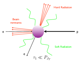
Figure 1: Schematic figure of the process e+pe+J+Xsuperscript𝑒𝑝superscript𝑒𝐽𝑋e^{-}+p\to e^{-}+J+X in the limit τ1PJTmuch-less-thansubscript𝜏1subscript𝑃subscript𝐽𝑇\tau_{1}\ll P_{J_{T}}. The restriction τ1PJTmuch-less-thansubscript𝜏1subscript𝑃subscript𝐽𝑇\tau_{1}\ll P_{J_{T}} (left panel) allows only soft radiation between the beam and jet directions. In the region of large 1-jettiness τ1PJTsimilar-tosubscript𝜏1subscript𝑃subscript𝐽𝑇\tau_{1}\sim P_{J_{T}} (right panel), additional hard radiation is allowed at wide angles from the leading jet and beam directions.

The 1-jettiness spectrum is characterized by two distinct regions as shown in Fig. 1. The region corresponding to τ1PJTmuch-less-thansubscript𝜏1subscript𝑃subscript𝐽𝑇\tau_{1}\ll P_{J_{T}} or τ1a1much-less-thansubscript𝜏1𝑎1\tau_{1a}\ll 1 corresponds to the left panel of Fig. 1 where the event is characterized by energetic radiation (EPJTsimilar-to𝐸subscript𝑃subscript𝐽𝑇E\sim P_{J_{T}} or EQ2similar-to𝐸superscript𝑄2E\sim\sqrt{Q^{2}}) only along the beam or jet directions and only soft radiation (Eτ1similar-to𝐸subscript𝜏1E\sim\tau_{1} or Eτ1aQ2similar-to𝐸subscript𝜏1𝑎superscript𝑄2E\sim\tau_{1a}\sqrt{Q^{2}}) at wide angles from the beam or jet directions. This can be understood from the definitions of τ1subscript𝜏1\tau_{1} and τ1asubscript𝜏1𝑎\tau_{1a} in Eqs. (4) and (7), respectively, where it is seen that the largest contributions come from energetic final state particles at wide angles from both the beam and jet directions. On the other hand, the final state particles with momenta closely aligned with the beam or jet reference vectors qBμsuperscriptsubscript𝑞𝐵𝜇q_{B}^{\mu} or qJμsuperscriptsubscript𝑞𝐽𝜇q_{J}^{\mu}, respectively, give small contributions.

The region of τ1PJTmuch-less-thansubscript𝜏1subscript𝑃subscript𝐽𝑇\tau_{1}\ll P_{J_{T}} or τ1a1much-less-thansubscript𝜏1𝑎1\tau_{1a}\ll 1 is referred to as the resummation region due to the presence of large Sudakov logarithms of the form αsnln2m(τ1/PJT)superscriptsubscript𝛼𝑠𝑛superscript2𝑚subscript𝜏1subscript𝑃subscript𝐽𝑇\alpha_{s}^{n}\ln^{2m}(\tau_{1}/P_{J_{T}}) or αsnln2m(τ1a)superscriptsubscript𝛼𝑠𝑛superscript2𝑚subscript𝜏1𝑎\alpha_{s}^{n}\ln^{2m}(\tau_{1a}), for mn𝑚𝑛m\leq n, that arise from the small 1-jettiness restriction on final state radiation and require resummation for making accurate predictions. The small 1-jettiness restriction effectively acts as a veto on additional energetic jets at wide angles from the beam or jet references vectors, qBμsuperscriptsubscript𝑞𝐵𝜇q_{B}^{\mu} or qJμsuperscriptsubscript𝑞𝐽𝜇q_{J}^{\mu}, respectively.

On the other hand, the region corresponding to τ1PJTsimilar-tosubscript𝜏1subscript𝑃subscript𝐽𝑇\tau_{1}\sim P_{J_{T}} or τ1a1less-than-or-similar-tosubscript𝜏1𝑎1\tau_{1a}\lesssim 1 corresponds to the right panel of Fig. 1, where the event is characterized by additional energetic radiation at wide angles from both the beam or leading jet directions. This corresponds to a looser veto on additional jets. In this region, the fixed order region, there are no large Sudakov logarithms so that resummation is not required and accurate predictions can be made using fixed order perturbative QCD calculations.

The resummation region, τ1PJTmuch-less-thansubscript𝜏1subscript𝑃subscript𝐽𝑇\tau_{1}\ll P_{J_{T}} or τ1a1much-less-thansubscript𝜏1𝑎1\tau_{1a}\ll 1, can be further classified into two sub-regions. The region ΛQCDτ1PJTmuch-less-thansubscriptΛ𝑄𝐶𝐷subscript𝜏1much-less-thansubscript𝑃subscript𝐽𝑇\Lambda_{QCD}\ll\tau_{1}\ll P_{J_{T}} or ΛQCD/Q2τ1a1much-less-thansubscriptΛ𝑄𝐶𝐷superscript𝑄2subscript𝜏1𝑎much-less-than1\Lambda_{QCD}/\sqrt{Q^{2}}\ll\tau_{1a}\ll 1 corresponds to the resummation region with perturbative soft radiation. The other region, τ1ΛQCDsimilar-tosubscript𝜏1subscriptΛ𝑄𝐶𝐷\tau_{1}\sim\Lambda_{QCD} or τ1aΛQCD/Q2similar-tosubscript𝜏1𝑎subscriptΛ𝑄𝐶𝐷superscript𝑄2\tau_{1a}\sim\Lambda_{QCD}/\sqrt{Q^{2}}, corresponds to the resummation region with non-perturbative soft radiation. In terms of the factorization theorem, the two regions correspondingly refer to a soft function that is either perturbatively calculable or is a non-perturbative function that is typically modeled for the purposes of generating numerical results. A constraint on the non-perturbative soft function model is that it smoothly reduces to the perturbative soft function as τ1subscript𝜏1\tau_{1} or τ1asubscript𝜏1𝑎\tau_{1a} is increased.

The three regions of the 1-jettiness spectrum discussed above are summarized in Table 1. The complete 1-jettiness spectrum with a matching of the resummation and fixed order regions is given by the standard schematic formula

dσ=[dσresumdσresumFO]+dσFO,𝑑𝜎delimited-[]𝑑subscript𝜎resum𝑑subscriptsuperscript𝜎FOresum𝑑superscript𝜎FO\displaystyle d\sigma=\left[d\sigma_{\rm resum}-d\sigma^{\rm FO}_{\rm resum}\right]+d\sigma^{\rm FO}, (18)

where dσresum𝑑subscript𝜎resumd\sigma_{\rm resum} denotes the resummed cross section in the region τ1PJTmuch-less-thansubscript𝜏1subscript𝑃subscript𝐽𝑇\tau_{1}\ll P_{J_{T}} or τ1a1much-less-thansubscript𝜏1𝑎1\tau_{1a}\ll 1, dσresumFO𝑑subscriptsuperscript𝜎FOresumd\sigma^{\rm FO}_{\rm resum} denotes this resummed cross section expanded to fixed order in perturbation theory, and dσFO𝑑superscript𝜎FOd\sigma^{\rm FO} denotes the full cross section at the same fixed order in perturbation theory. The expanded resummed cross section dσresumFO𝑑subscriptsuperscript𝜎FOresumd\sigma^{\rm FO}_{\rm resum} differs from the full fixed order cross section dσFO𝑑superscript𝜎FOd\sigma^{\rm FO} by terms that are non-singular in the τ10subscript𝜏10\tau_{1}\to 0 or τ1a0subscript𝜏1𝑎0\tau_{1a}\to 0 limit. The formula in Eq. (18) has the required properties for generating a smooth and continuous spectrum across the resummation and fixed order regions. In particular, we see that in the singular limit τ10subscript𝜏10\tau_{1}\to 0 or τ1a0subscript𝜏1𝑎0\tau_{1a}\to 0, the cross section is dominated by the resummed cross section dσresum𝑑subscript𝜎resumd\sigma_{\rm resum} due to a cancellation between dσresumFO𝑑subscriptsuperscript𝜎FOresumd\sigma^{\rm FO}_{\rm resum} and dσFO𝑑superscript𝜎FOd\sigma^{\rm FO} up to suppressed non-singular terms. On the other hand, in the fixed order region τ1PJTsimilar-tosubscript𝜏1subscript𝑃subscript𝐽𝑇\tau_{1}\sim P_{J_{T}} or τ1a1less-than-or-similar-tosubscript𝜏1𝑎1\tau_{1a}\lesssim 1, the cross section is dominated by the full fixed order cross section dσFO𝑑superscript𝜎FOd\sigma^{\rm FO} due to a cancellation between dσresum𝑑subscript𝜎resumd\sigma_{\rm resum} and dσresumFO𝑑subscriptsuperscript𝜎FOresumd\sigma^{\rm FO}_{\rm resum} up to terms suppressed in perturbation theory.

In the rest of the section, we discuss the features of the resummation and fixed order regions in more detail before providing numerical results.

Regions τ1subscript𝜏1\tau_{1} τ1asubscript𝜏1𝑎\tau_{1a}
Resummation Region τ1ΛQCDsimilar-tosubscript𝜏1subscriptΛQCD\tau_{1}\sim\Lambda_{{\rm QCD}} τ1aΛQCD/Q2similar-tosubscript𝜏1𝑎subscriptΛ𝑄𝐶𝐷superscript𝑄2\tau_{1a}\sim\>\>\Lambda_{QCD}/\sqrt{Q^{2}}
(nonperturbative soft radiation)
Resummation Region ΛQCDτ1PJTmuch-less-thansubscriptΛ𝑄𝐶𝐷subscript𝜏1much-less-thansubscript𝑃subscript𝐽𝑇\>\>\Lambda_{QCD}\ll\tau_{1}\ll P_{J_{T}}\>\> ΛQCD/Q2τ1a1much-less-thansubscriptΛ𝑄𝐶𝐷superscript𝑄2subscript𝜏1𝑎much-less-than1\>\>\Lambda_{QCD}/\sqrt{Q^{2}}\ll\tau_{1a}\ll 1\>\>
(perturbative soft radiation)
Fixed Order Region τ1PJTsimilar-tosubscript𝜏1subscript𝑃subscript𝐽𝑇\tau_{1}\sim P_{J_{T}} τ1a1less-than-or-similar-tosubscript𝜏1𝑎1\tau_{1a}\lesssim 1
Table 1: The three distinct regions in the τ1subscript𝜏1\tau_{1} and τ1asubscript𝜏1𝑎\tau_{1a} 1-jettiness spectra.

III.1 Resummation Region

The resummation region, characterized by the conditions

τ1PJT,orτ1a1,formulae-sequencemuch-less-thansubscript𝜏1subscript𝑃subscript𝐽𝑇ormuch-less-thansubscript𝜏1𝑎1\displaystyle\tau_{1}\ll P_{J_{T}},\qquad\text{or}\qquad\tau_{1a}\ll 1, (19)

allows for writing down a factorization formula that is systematically improvable, facilitates the resummation of large Sudakov logarithms, and is independent of the external jet algorithm used to determine the jet reference vector qJμsuperscriptsubscript𝑞𝐽𝜇q_{J}^{\mu} in Eq. (6). For the purposes of discussing and demonstrating the jet algorithm independence, it is more convenient and natural to work with the observable dσ[τ1,PJT,yJ]𝑑𝜎subscript𝜏1subscript𝑃subscript𝐽𝑇subscript𝑦𝐽d\sigma\left[\tau_{1},P_{J_{T}},y_{J}\right], since it is differential in the PJTsubscript𝑃subscript𝐽𝑇P_{J_{T}} and yJsubscript𝑦𝐽y_{J} variables that are directly related to the properties of the leading jet.

We can understand the external jet algorithm independence in the resummation region, τ1PJTmuch-less-thansubscript𝜏1subscript𝑃subscript𝐽𝑇\tau_{1}\ll P_{J_{T}}, by noting that in this region the typical event configurations look like the left panel of Fig. 1. These events are characterized by a single hard jet that is well separated from the beam region with only soft radiation between the beam and jet directions. For such events, the resulting difference between different jet algorithms just corresponds to the amount of soft radiation clustered with the jet. Only the jet mass is sensitive to the amount of soft radiation. In particular, its transverse momentum KJTsubscript𝐾subscript𝐽𝑇K_{J_{T}} and rapidity yKsubscript𝑦𝐾y_{K} are not affected by the soft radiation, up to power corrections in τ1/PJTsubscript𝜏1subscript𝑃subscript𝐽𝑇\tau_{1}/P_{J_{T}}. Thus, in the resummation region τ1PJTmuch-less-thansubscript𝜏1subscript𝑃subscript𝐽𝑇\tau_{1}\ll P_{J_{T}}, the reference vector qJμsuperscriptsubscript𝑞𝐽𝜇q_{J}^{\mu} in Eq. (6) is independent of the external jet algorithm used to find the leading jet. Correspondingly, the resulting values of the 1-jettiness event shape τ1subscript𝜏1\tau_{1} and the 1-jettiness jet momentum PJμsuperscriptsubscript𝑃𝐽𝜇P_{J}^{\mu}, according to Eqs. (4) and (9), respectively, are also independent of the external jet algorithm. Furthermore, we have PJT=KJTsubscript𝑃subscript𝐽𝑇subscript𝐾subscript𝐽𝑇P_{J_{T}}=K_{J_{T}} and yJ=yKsubscript𝑦𝐽subscript𝑦𝐾y_{J}=y_{K}, up to power corrections in τ1/PJTsubscript𝜏1subscript𝑃subscript𝐽𝑇\tau_{1}/P_{J_{T}}. Thus, in the resummation region, Eq. (6) can be written as

qJ|τ1PJT(PJTcoshyJ,PJT,PJTsinhyJ),QJ2PJTcoshyJ.formulae-sequencesimilar-to-or-equalsevaluated-atsubscript𝑞𝐽much-less-thansubscript𝜏1subscript𝑃subscript𝐽𝑇subscript𝑃subscript𝐽𝑇coshsubscript𝑦𝐽subscript𝑃subscript𝐽𝑇subscript𝑃subscript𝐽𝑇sinhsubscript𝑦𝐽similar-to-or-equalssubscript𝑄𝐽2subscript𝑃subscript𝐽𝑇coshsubscript𝑦𝐽\displaystyle q_{J}\Big{|}_{\tau_{1}\ll P_{J_{T}}}\simeq(P_{J_{T}}{\rm cosh}y_{J},\vec{P}_{J_{T}},P_{J_{T}}{\rm sinh}y_{J}),\qquad Q_{J}\simeq 2P_{J_{T}}{\rm cosh}y_{J}. (20)

Thus, for a priori specified values of PJTsubscript𝑃subscript𝐽𝑇P_{J_{T}} and yJsubscript𝑦𝐽y_{J}, we can unambiguously compute dσresum[τ1,PJT,yJ]𝑑subscript𝜎resumsubscript𝜏1subscript𝑃subscript𝐽𝑇subscript𝑦𝐽d\sigma_{\rm resum}\left[\tau_{1},P_{J_{T}},y_{J}\right] using Eq. (20) in Eq. (4), without any reference to an external jet algorithm.

Furthermore, in this resummation region where the final jet is initiated by the quark or anti-quark emerging from the hard scattering followed by a parton shower, one can associate the leading jet momentum as PJ=q+xPsubscript𝑃𝐽𝑞𝑥𝑃P_{J}=q+xP, up to power corrections from ambient soft radiation clustered with the jet. In general, there will be some uncertainty in applying this relationship arising from QED photon emissions by the initial and final electron that affects the reconstruction Kripfganz:1991 ; BLUMLEIN2003242 ; Afanasev:2004 ; Liu:2020rvc of qμsuperscript𝑞𝜇q^{\mu}, and correspondingly the (Q2,x)superscript𝑄2𝑥(Q^{2},x) values at the primary electron scattering vertex. The identification PJ=q+xPsubscript𝑃𝐽𝑞𝑥𝑃P_{J}=q+xP implies a simple relationship between dσresum[τ1,PJT,yJ]𝑑subscript𝜎resumsubscript𝜏1subscript𝑃subscript𝐽𝑇subscript𝑦𝐽d\sigma_{\rm resum}\left[\tau_{1},P_{J_{T}},y_{J}\right] and dσresum[τ1a,Q2,y]𝑑subscript𝜎resumsubscript𝜏1𝑎superscript𝑄2𝑦d\sigma_{\rm resum}\left[\tau_{1a},Q^{2},y\right] or dσresum[τ1a,Q2,x]𝑑subscript𝜎resumsubscript𝜏1𝑎superscript𝑄2𝑥d\sigma_{\rm resum}\left[\tau_{1a},Q^{2},x\right] to all orders in perturbative QCD. This relationship, as derived in appendix A, is given by

dσresum[τ1a,Q2,y]=𝑑subscript𝜎resumsubscript𝜏1𝑎superscript𝑄2𝑦absent\displaystyle d\sigma_{\rm resum}\left[\tau_{1a},Q^{2},y\right]=
1y2ydσresum[τ1=Q2τ1a,PJT=Q2(1y),yJ=12lnQ2(1y)y2s].1𝑦2𝑦𝑑subscript𝜎resumdelimited-[]formulae-sequencesubscript𝜏1superscript𝑄2subscript𝜏1𝑎formulae-sequencesubscript𝑃subscript𝐽𝑇superscript𝑄21𝑦subscript𝑦𝐽12superscript𝑄21𝑦superscript𝑦2𝑠\displaystyle\frac{\sqrt{1-y}}{2y}\>d\sigma_{\rm resum}\left[\tau_{1}=\sqrt{Q^{2}}\>\tau_{1a},P_{J_{T}}=\sqrt{Q^{2}(1-y)},y_{J}=\frac{1}{2}\ln\frac{Q^{2}(1-y)}{y^{2}s}\right]. (21)

The factorization formula for dσresum[τ1a,Q2,x]𝑑subscript𝜎resumsubscript𝜏1𝑎superscript𝑄2𝑥d\sigma_{\rm resum}\left[\tau_{1a},Q^{2},x\right] is then simply obtained from dσresum[τ1a,Q2,y]𝑑subscript𝜎resumsubscript𝜏1𝑎superscript𝑄2𝑦d\sigma_{\rm resum}\left[\tau_{1a},Q^{2},y\right] using the general relation in Eq. (II). One can easily check these relations for the tree level cross sections given in Eqs. (13) and (16).

Thus, in the rest of this section, when discussing the resummation region, we will primarily focus on dσresum[τ1,PJT,yJ]𝑑subscript𝜎resumsubscript𝜏1subscript𝑃subscript𝐽𝑇subscript𝑦𝐽d\sigma_{\rm resum}\left[\tau_{1},P_{J_{T}},y_{J}\right] with the understanding that dσresum[τ1a,Q2,y]𝑑subscript𝜎resumsubscript𝜏1𝑎superscript𝑄2𝑦d\sigma_{\rm resum}\left[\tau_{1a},Q^{2},y\right] and dσresum[τ1a,Q2,x]𝑑subscript𝜎resumsubscript𝜏1𝑎superscript𝑄2𝑥d\sigma_{\rm resum}\left[\tau_{1a},Q^{2},x\right] can then be easily obtained from the relationships in Eqs. (III.1) and the second line in Eq. (II), respectively.

In Refs. Kang:2012zr ; Kang:2013wca , it was shown the factorization formula for dσresum[τ1,PJT,yJ]𝑑subscript𝜎resumsubscript𝜏1subscript𝑃subscript𝐽𝑇subscript𝑦𝐽d\sigma_{\rm resum}\left[\tau_{1},P_{J_{T}},y_{J}\right] has the schematic form

dσresum[τ1,PJT,yJ]𝑑subscript𝜎resumsubscript𝜏1subscript𝑃subscript𝐽𝑇subscript𝑦𝐽\displaystyle d\sigma_{\rm resum}\left[\tau_{1},P_{J_{T}},y_{J}\right] similar-to\displaystyle\sim HBJ𝒮,tensor-product𝐻𝐵𝐽𝒮\displaystyle H\otimes B\otimes J\otimes{\cal S}, (22)

where H𝐻H is the hard function describing the physics of the hard scattering, B𝐵B is the beam function Stewart:2009yx describing the physics of the perturbative collinear initial state radiation along the beam direction and the initial state PDF, J𝐽J is the quark jet function describing the physics of the collinear radiation along the jet direction, and 𝒮𝒮{\cal S} is the soft function describing the physics of the soft radiation throughout the event. The beam function can be further factored into a perturbatively calculable coefficient and initial state PDFs

Bf,similar-to𝐵tensor-product𝑓\displaystyle B\sim{\cal I}\otimes f, (23)

where {\cal I} describes the perturbative initial state collinear radiation along the beam direction. Each of these functions in the factorization formula is sensitive to physics associated with a single energy scale so that one can minimize large logarithms by choosing the corresponding renormalization scales to have the scaling

μHPJT,μJμBτ1PJT,μSτ1.formulae-sequenceformulae-sequencesimilar-tosubscript𝜇𝐻subscript𝑃subscript𝐽𝑇similar-tosubscript𝜇𝐽subscript𝜇𝐵similar-tosubscript𝜏1subscript𝑃subscript𝐽𝑇similar-tosubscript𝜇𝑆subscript𝜏1\displaystyle\mu_{H}\sim P_{J_{T}},\>\>\>\mu_{J}\sim\mu_{B}\sim\sqrt{\tau_{1}P_{J_{T}}},\>\>\>\mu_{S}\sim\tau_{1}. (24)

Correspondingly, for the τ1asubscript𝜏1𝑎\tau_{1a} observable, the renormalization scales chosen to minimize large logarithms have the scaling

μHQ2,μJμBτ1aQ2,μSτ1aQ2.formulae-sequenceformulae-sequencesimilar-tosubscript𝜇𝐻superscript𝑄2similar-tosubscript𝜇𝐽subscript𝜇𝐵similar-tosubscript𝜏1𝑎superscript𝑄2similar-tosubscript𝜇𝑆subscript𝜏1𝑎superscript𝑄2\displaystyle\mu_{H}\sim\sqrt{Q^{2}},\>\>\>\mu_{J}\sim\mu_{B}\sim\sqrt{\tau_{1a}Q^{2}},\>\>\>\mu_{S}\sim\tau_{1a}\sqrt{Q^{2}}. (25)

Using the renormalization group equations in SCET, the hard, beam, jet, and soft functions are evolved to the common scale μ𝜇\mu at which the cross section is evaluated. In the process, large logarithms of τ1/PJTsubscript𝜏1subscript𝑃subscript𝐽𝑇\tau_{1}/P_{J_{T}} or τ1asubscript𝜏1𝑎\tau_{1a} are resummed in the corresponding resummation region τ1PJTmuch-less-thansubscript𝜏1subscript𝑃subscript𝐽𝑇\tau_{1}\ll P_{J_{T}} or τ1a1much-less-thansubscript𝜏1𝑎1\tau_{1a}\ll 1, respectively.

III.2 Momentum Space Resummation Factorization Formula

The detailed form of the factorization formula Kang:2012zr ; Kang:2013wca in the resummation region, τ1PJTmuch-less-thansubscript𝜏1subscript𝑃subscript𝐽𝑇\tau_{1}\ll P_{J_{T}}, is given by

dσresum[τ1,PJT,yJ]𝑑subscript𝜎resumsubscript𝜏1subscript𝑃subscript𝐽𝑇subscript𝑦𝐽\displaystyle d\sigma_{\rm resum}\left[\tau_{1},P_{J_{T}},y_{J}\right] =\displaystyle= σ0H(ξ2,μ;μH)𝑑sJ𝑑tBJ(sJ,μ;μJ)𝒮(τ1tBQBsJQJ,μ;μS)subscript𝜎0𝐻superscript𝜉2𝜇subscript𝜇𝐻differential-dsubscript𝑠𝐽differential-dsubscript𝑡𝐵𝐽subscript𝑠𝐽𝜇subscript𝜇𝐽𝒮subscript𝜏1subscript𝑡𝐵subscript𝑄𝐵subscript𝑠𝐽subscript𝑄𝐽𝜇subscript𝜇𝑆\displaystyle\sigma_{0}\>H(\xi^{2},\mu;\mu_{H})\int ds_{J}\int dt_{B}\>J(s_{J},\mu;\mu_{J}){\cal S}\left(\tau_{1}-\frac{t_{B}}{Q_{B}}-\frac{s_{J}}{Q_{J}},\mu;\mu_{S}\right) (26)
×[qLqBq(tB,x,μ;μB)+q¯Lq¯Bq¯(tB,x,μ;μB)],absentdelimited-[]subscript𝑞subscript𝐿𝑞subscript𝐵𝑞subscript𝑡𝐵subscript𝑥𝜇subscript𝜇𝐵subscript¯𝑞subscript𝐿¯𝑞subscript𝐵¯𝑞subscript𝑡𝐵subscript𝑥𝜇subscript𝜇𝐵\displaystyle\times\left[\sum_{q}L_{q}\>B_{q}(t_{B},x_{*},\mu;\mu_{B})+\sum_{\bar{q}}L_{\bar{q}}\>B_{\bar{q}}(t_{B},x_{*},\mu;\mu_{B})\right],

where σ0subscript𝜎0\sigma_{0} and xsubscript𝑥x_{*} are given in Eq. (17) and we have defined

ξ2xsPJTeyJ=PJT21PJTseyJ.superscript𝜉2subscript𝑥𝑠subscript𝑃subscript𝐽𝑇superscript𝑒subscript𝑦𝐽superscriptsubscript𝑃subscript𝐽𝑇21subscript𝑃subscript𝐽𝑇𝑠superscript𝑒subscript𝑦𝐽\displaystyle\xi^{2}\equiv x_{*}\sqrt{s}P_{J_{T}}e^{-y_{J}}=\frac{P_{J_{T}}^{2}}{1-\frac{P_{J_{T}}}{\sqrt{s}}\>e^{-y_{J}}}. (27)

The quark or anti-quark beam functions (Bq,q¯subscript𝐵𝑞¯𝑞B_{q,\bar{q}}) are matched Stewart:2009yx onto the PDFs as

Bq,q¯(tB,x,μ;μB)subscript𝐵𝑞¯𝑞subscript𝑡𝐵𝑥𝜇subscript𝜇𝐵\displaystyle B_{q,\bar{q}}(t_{B},x,\mu;\mu_{B}) =\displaystyle= ix1dzz(q,q¯)i(tB,xz,μ;μB)fi/p(z,μB),subscript𝑖superscriptsubscript𝑥1𝑑𝑧𝑧subscript𝑞¯𝑞𝑖subscript𝑡𝐵𝑥𝑧𝜇subscript𝜇𝐵subscript𝑓𝑖𝑝𝑧subscript𝜇𝐵\displaystyle\sum_{i}\int_{x}^{1}\frac{dz}{z}{\cal I}_{({q,\bar{q}})i}\left(t_{B},\frac{x}{z},\mu;\mu_{B}\right)f_{i/p}(z,\mu_{B}), (28)

where the qisubscript𝑞𝑖{\cal I}_{qi} or q¯isubscript¯𝑞𝑖{\cal I}_{\bar{q}i} are perturbatively calculable matching coefficients and the index i𝑖i runs over the possible initial parton species in the proton, including the quarks, the anti-quarks, and the gluon. The factorization formula presented in Refs. Kang:2012zr ; Kang:2013wca , explicitly included only the case of single photon exchange in the hard scattering. The result in Eq. (26) is extended to also include the contribution from single Z𝑍Z-boson exchange in the hard scattering through the Lq,q¯subscript𝐿𝑞¯𝑞L_{q,\bar{q}} coefficients Kang:2013nha . Note that the hard, jet, beam, and soft functions include their renormalization group evolution from their natural scales μH,μJ,μBsubscript𝜇𝐻subscript𝜇𝐽subscript𝜇𝐵\mu_{H},\mu_{J},\mu_{B}, and μSsubscript𝜇𝑆\mu_{S}, respectively, to the common scale μ𝜇\mu. The PDF in Eq. (28) is evaluated at the μBsubscript𝜇𝐵\mu_{B} scale using the standard DGLAP evolution. By charge conjugation and quark flavor symmetry of QCD, the quark jet function J𝐽J is the same for all light quark and anti-quark flavors so that Jq(sJ,μ;μJ)=Jq¯(sJ,μ;μJ)J(sJ,μ;μJ)subscript𝐽𝑞subscript𝑠𝐽𝜇subscript𝜇𝐽subscript𝐽¯𝑞subscript𝑠𝐽𝜇subscript𝜇𝐽𝐽subscript𝑠𝐽𝜇subscript𝜇𝐽J_{q}(s_{J},\mu;\mu_{J})=J_{\bar{q}}(s_{J},\mu;\mu_{J})\equiv J(s_{J},\mu;\mu_{J}) and is thus factored out of the sum over quark and anti-quark flavors. The soft function appearing in Eq. (26) is defined in terms of the generalized hemisphere soft function Bauer:2003di ; Jouttenus:2011wh as

𝒮(τ1,μ;μS)𝒮subscript𝜏1𝜇subscript𝜇𝑆\displaystyle{\cal S}\left(\tau_{1},\mu;\mu_{S}\right) =\displaystyle= 𝑑kB𝑑kJδ(τ1kBkJ)𝒮(kB,kJ,μ;μS).differential-dsubscript𝑘𝐵differential-dsubscript𝑘𝐽𝛿subscript𝜏1subscript𝑘𝐵subscript𝑘𝐽𝒮subscript𝑘𝐵subscript𝑘𝐽𝜇subscript𝜇𝑆\displaystyle\int dk_{B}\int dk_{J}\>\delta(\tau_{1}-k_{B}-k_{J})\>{\cal S}(k_{B},k_{J},\mu;\mu_{S}). (29)

The generalized hemisphere soft function 𝒮(kB,kJ,μ;μS)𝒮subscript𝑘𝐵subscript𝑘𝐽𝜇subscript𝜇𝑆{\cal S}(k_{B},k_{J},\mu;\mu_{S}), appearing on the RHS above, is a function of two kinematic arguments kB,kJsubscript𝑘𝐵subscript𝑘𝐽k_{B},k_{J}, corresponding to the contribution to τ1subscript𝜏1\tau_{1} of soft radiation grouped with the nuclear beam and jet directions respectively, as determined by the 1-jettiness algorithm used to calculate τ1subscript𝜏1\tau_{1} in Eq.(4).

In the region μSτ1ΛQCDsimilar-tosubscript𝜇𝑆subscript𝜏1similar-tosubscriptΛ𝑄𝐶𝐷\mu_{S}\sim\tau_{1}\sim\Lambda_{QCD}, the soft function becomes non-perturbative and is modeled as a convolution between the perturbatively calculable partonic soft function and a phenomenological model function (Fmod.subscript𝐹modF_{\rm mod.}) as

𝒮(τ1,μS)=𝑑u𝒮part.(τ1u,μS)Fmod.(u),𝒮subscript𝜏1subscript𝜇𝑆differential-d𝑢subscript𝒮partsubscript𝜏1𝑢subscript𝜇𝑆subscript𝐹mod𝑢\displaystyle{\cal S}(\tau_{1},\mu_{S})=\int du\>{\cal S}_{\rm part.}(\tau_{1}-u,\mu_{S})\>F_{{\rm mod.}}(u), (30)

with the normalization condition

𝑑uFmod.(u)=1.differential-d𝑢subscript𝐹mod𝑢1\displaystyle\int du\>F_{{\rm mod.}}(u)=1. (31)

This convolution structure ensures that the soft function reduces to the perturbative partonic soft function in the region τ1ΛQCDmuch-greater-thansubscript𝜏1subscriptΛ𝑄𝐶𝐷\tau_{1}\gg\Lambda_{QCD}, up to power corrections in ΛQCD/τ1subscriptΛ𝑄𝐶𝐷subscript𝜏1\Lambda_{QCD}/\tau_{1}. We choose a default parameterization for Fmod.(u)subscript𝐹mod𝑢F_{{\rm mod.}}(u) as

Fmod.(u)=N(a,b,Λ)Λ(uΛ)a1Exp[(ub)2Λ2],subscript𝐹mod𝑢𝑁𝑎𝑏ΛΛsuperscript𝑢Λ𝑎1Expdelimited-[]superscript𝑢𝑏2superscriptΛ2\displaystyle F_{{\rm mod.}}(u)=\frac{N(a,b,\Lambda)}{\Lambda}\left(\frac{u}{\Lambda}\right)^{a-1}{\rm Exp}\left[-\frac{(u-b)^{2}}{\Lambda^{2}}\right], (32)

where a,b,𝑎𝑏a,b, and ΛΛ\Lambda are free parameters and N(a,b,Λ)𝑁𝑎𝑏ΛN(a,b,\Lambda) is a normalization factor that ensures the normalization constraint in Eq. (31). We note that in general, the non-perturbative soft function effects will be different for the τ1subscript𝜏1\tau_{1} and τ1asubscript𝜏1𝑎\tau_{1a} distributions. This difference can arise because of the difference in the measurement function at the operator level for the non-perturbative soft function, corresponding to the difference in the definitions of τ1subscript𝜏1\tau_{1} and τ1asubscript𝜏1𝑎\tau_{1a}, as seen in Eqs. (4) and (7), respectively. For simplicity, in this work, we choose to also implement non-perturbative effects for τ1asubscript𝜏1𝑎\tau_{1a} by just using the non-perturbative model parameterization in Eq. (32), but with appropriately different values for the a,b,𝑎𝑏a,b, and ΛΛ\Lambda parameters, and using Eq. (III.1).

III.3 Position Space Resummation Factorization Formula

The factorization formula in Eqs. (26) and (28) can be written in terms of the Fourier transformed position space objects. The momentum space beam, jet, and soft functions are related to their position space counterparts by the Fourier transforms

(q,q¯)i(tB,x,μB)subscript𝑞¯𝑞𝑖subscript𝑡𝐵𝑥subscript𝜇𝐵\displaystyle{\cal I}_{(q,\bar{q})i}(t_{B},x,\mu_{B}) =\displaystyle= dyB2πeiyBtB(q,q¯)i(yB,x,μB),𝑑subscript𝑦𝐵2𝜋superscript𝑒𝑖subscript𝑦𝐵subscript𝑡𝐵subscript𝑞¯𝑞𝑖subscript𝑦𝐵𝑥subscript𝜇𝐵\displaystyle\int\frac{dy_{B}}{2\pi}\>e^{iy_{B}t_{B}}{\cal I}_{(q,\bar{q})i}(y_{B},x,\mu_{B}),
J(sJ,μJ)𝐽subscript𝑠𝐽subscript𝜇𝐽\displaystyle J(s_{J},\mu_{J}) =\displaystyle= dyJ2πeiyJsJJ(yJ,μJ),𝑑subscript𝑦𝐽2𝜋superscript𝑒𝑖subscript𝑦𝐽subscript𝑠𝐽𝐽subscript𝑦𝐽subscript𝜇𝐽\displaystyle\int\frac{dy_{J}}{2\pi}\>e^{iy_{J}s_{J}}J(y_{J},\mu_{J}), (33)
𝒮(τ1,μS)𝒮subscript𝜏1subscript𝜇𝑆\displaystyle{\cal S}(\tau_{1},\mu_{S}) =\displaystyle= dyS2πeiySτ1𝒮(yS,μS).𝑑subscript𝑦𝑆2𝜋superscript𝑒𝑖subscript𝑦𝑆subscript𝜏1𝒮subscript𝑦𝑆subscript𝜇𝑆\displaystyle\int\frac{dy_{S}}{2\pi}\>e^{iy_{S}\tau_{1}}\>{\cal S}(y_{S},\mu_{S}).

In position space, the renormalization group evolution becomes multiplicative so that the beam, jet, and soft functions can be evolved to the common scale μ𝜇\mu from their natural scales at μB,μJ,subscript𝜇𝐵subscript𝜇𝐽\mu_{B},\mu_{J}, and μSsubscript𝜇𝑆\mu_{S}, respectively, as

(q,q¯)i(yB,x,μ;μB)subscript𝑞¯𝑞𝑖subscript𝑦𝐵𝑥𝜇subscript𝜇𝐵\displaystyle{\cal I}_{(q,\bar{q})i}(y_{B},x,\mu;\mu_{B}) =\displaystyle= UB(yB,μ,μB)(q,q¯)i(yB,x,μB),subscript𝑈𝐵subscript𝑦𝐵𝜇subscript𝜇𝐵subscript𝑞¯𝑞𝑖subscript𝑦𝐵𝑥subscript𝜇𝐵\displaystyle U_{B}(y_{B},\mu,\mu_{B})\>{\cal I}_{(q,\bar{q})i}(y_{B},x,\mu_{B}),
J(yJ,μ;μJ)𝐽subscript𝑦𝐽𝜇subscript𝜇𝐽\displaystyle J(y_{J},\mu;\mu_{J}) =\displaystyle= UJ(yJ,μ,μJ)J(yJ,μJ),subscript𝑈𝐽subscript𝑦𝐽𝜇subscript𝜇𝐽𝐽subscript𝑦𝐽subscript𝜇𝐽\displaystyle U_{J}(y_{J},\mu,\mu_{J})\>J(y_{J},\mu_{J}), (34)
𝒮(yS,μ;μS)𝒮subscript𝑦𝑆𝜇subscript𝜇𝑆\displaystyle{\cal S}(y_{S},\mu;\mu_{S}) =\displaystyle= US(yS,μ,μS)𝒮(yS,μS),subscript𝑈𝑆subscript𝑦𝑆𝜇subscript𝜇𝑆𝒮subscript𝑦𝑆subscript𝜇𝑆\displaystyle U_{S}(y_{S},\mu,\mu_{S}){\cal S}(y_{S},\mu_{S}),

where UB(yB,μ,μB),UJ(yJ,μ,μJ),subscript𝑈𝐵subscript𝑦𝐵𝜇subscript𝜇𝐵subscript𝑈𝐽subscript𝑦𝐽𝜇subscript𝜇𝐽U_{B}(y_{B},\mu,\mu_{B}),U_{J}(y_{J},\mu,\mu_{J}), and US(yS,μ,μS)subscript𝑈𝑆subscript𝑦𝑆𝜇subscript𝜇𝑆U_{S}(y_{S},\mu,\mu_{S}) are the position space evolution factors for the beam, jet, and soft functions, respectively. Similarly, the hard function also has a multiplicative renormalization group evolution

H(ξ2,μ;μH)𝐻superscript𝜉2𝜇subscript𝜇𝐻\displaystyle H(\xi^{2},\mu;\mu_{H}) =\displaystyle= UH(ξ2,μ,μH)H(ξ2,μH),subscript𝑈𝐻superscript𝜉2𝜇subscript𝜇𝐻𝐻superscript𝜉2subscript𝜇𝐻\displaystyle U_{H}(\xi^{2},\mu,\mu_{H})H(\xi^{2},\mu_{H}), (35)

where UH(ξ2,μ,μH)subscript𝑈𝐻superscript𝜉2𝜇subscript𝜇𝐻U_{H}(\xi^{2},\mu,\mu_{H}) is the corresponding hard function renormalization group evolution factor.

Furthermore, the momentum space convolution between the partonic soft function and the model function in Eq. (30) becomes a simple product in position space

𝒮(yτ,μS)𝒮subscript𝑦𝜏subscript𝜇𝑆\displaystyle{\cal S}(y_{\tau},\mu_{S}) =\displaystyle= 𝒮part.(yτ,μS)Fmod.(yτ),subscript𝒮partsubscript𝑦𝜏subscript𝜇𝑆subscript𝐹modsubscript𝑦𝜏\displaystyle{\cal S}_{\rm part.}(y_{\tau},\mu_{S})\>F_{{\rm mod.}}(y_{\tau}), (36)

where the position space model function is given by the Fourier transform

Fmod.(yτ)=𝑑ueiyτuFmod.(u).subscript𝐹modsubscript𝑦𝜏differential-d𝑢superscript𝑒𝑖subscript𝑦𝜏𝑢subscript𝐹mod𝑢\displaystyle F_{{\rm mod.}}(y_{\tau})=\int du\>e^{-iy_{\tau}u}\>F_{{\rm mod.}}(u). (37)

In terms of these position space objects, the factorization formula in Eq. (26) now takes the form

dσresum[τ1,PJT,yJ]𝑑subscript𝜎resumsubscript𝜏1subscript𝑃subscript𝐽𝑇subscript𝑦𝐽\displaystyle d\sigma_{\rm resum}\left[\tau_{1},P_{J_{T}},y_{J}\right] =\displaystyle= σ0UH(ξ2,μ,μH)H(ξ2,μH)subscript𝜎0subscript𝑈𝐻superscript𝜉2𝜇subscript𝜇𝐻𝐻superscript𝜉2subscript𝜇𝐻\displaystyle\sigma_{0}\>U_{H}(\xi^{2},\mu,\mu_{H})H(\xi^{2},\mu_{H})
×dyτ2πeiyττ1UJ(yτQJ,μ,μJ)US(yτ,μ,μS)UB(yτQa,μ,μB)\displaystyle\times\int\frac{dy_{\tau}}{2\pi}e^{iy_{\tau}\tau_{1}}U_{J}(\frac{y_{\tau}}{Q_{J}},\mu,\mu_{J})U_{S}(y_{\tau},\mu,\mu_{S})U_{B}(\frac{y_{\tau}}{Q_{a}},\mu,\mu_{B})
×J(yτQJ,μJ)𝒮part.(yτ,μS)Fmod.(yτ)absent𝐽subscript𝑦𝜏subscript𝑄𝐽subscript𝜇𝐽subscript𝒮partsubscript𝑦𝜏subscript𝜇𝑆subscript𝐹modsubscript𝑦𝜏\displaystyle\times J(\frac{y_{\tau}}{Q_{J}},\mu_{J})\>{\cal S}_{\rm part.}(y_{\tau},\mu_{S})\>F_{{\rm mod.}}(y_{\tau})
×[qiLqx1dzzqi(yτQB,xz,μB)fi/p(z,μB)\displaystyle\times\Big{[}\sum_{q}\sum_{i}L_{q}\int_{x_{*}}^{1}\frac{dz}{z}\>{\cal I}_{qi}\left(\frac{y_{\tau}}{Q_{B}},\frac{x_{*}}{z},\mu_{B}\right)f_{i/p}(z,\mu_{B})
+q¯iLq¯x1dzzq¯i(yτQB,xz,μB)fi/p(z,μB)],\displaystyle+\sum_{\bar{q}}\sum_{i}L_{\bar{q}}\int_{x_{*}}^{1}\frac{dz}{z}\>{\cal I}_{\bar{q}i}\left(\frac{y_{\tau}}{Q_{B}},\frac{x_{*}}{z},\mu_{B}\right)f_{i/p}(z,\mu_{B})\Big{]},

where all the hard, beam, jet, and soft functions are evaluated at their natural scales and the explicit renormalization group evolution factors evolve them to the common scale μ𝜇\mu.

More details of the factorization formula in Eq. (III.3) can be found in the appendices D, C, and E which give explicit expressions for the various RG evolution factors up to N3LL, explicit expressions for the hard, beam, jet, and soft functions up to NNLO, and a master factorization formula useful for numerical implementation, respectively.

III.4 Profile functions

As discussed in Refs. Berger:2010xi and Stewart:2011cf , one must be careful in estimating the perturbative uncertainty in the matched spectrum of Eq. (18). In particular, the fixed order contribution dσFO𝑑superscript𝜎𝐹𝑂d\sigma^{FO}, appropriate in the fixed-order region where τ1PJTsimilar-tosubscript𝜏1subscript𝑃subscript𝐽𝑇\tau_{1}\sim P_{J_{T}} or τ1a1similar-tosubscript𝜏1𝑎1\tau_{1a}\sim 1, depends on the single common scale, μFOsubscript𝜇FO\mu_{\rm FO}. On the other hand, the resummed cross section depends on multiple scales; the hard function scale μHμFOsimilar-tosubscript𝜇𝐻subscript𝜇FO\mu_{H}\sim\mu_{\rm FO} and the beam, jet, and soft function scales, μB,μJ,subscript𝜇𝐵subscript𝜇𝐽\mu_{B},\mu_{J}, and μSsubscript𝜇𝑆\mu_{S}, respectively. These are the scales that correspondingly minimize large logarithms in the hard, beam, jet, and soft functions. The matched spectrum should approach the fixed order result, dσFO𝑑superscript𝜎𝐹𝑂d\sigma^{FO}, in the fixed order region. This requires that resummation turns off as one approaches the fixed order region and the scales μB,μJ,subscript𝜇𝐵subscript𝜇𝐽\mu_{B},\mu_{J}, and μSsubscript𝜇𝑆\mu_{S} smoothly converge to μFOμHsimilar-tosubscript𝜇𝐹𝑂subscript𝜇H\mu_{FO}\sim\mu_{\rm H}. This is done by introducing profile functions Kang:2013nha which make the scales μB,μJ,subscript𝜇𝐵subscript𝜇𝐽\mu_{B},\mu_{J}, and μSsubscript𝜇𝑆\mu_{S} functions of τ1subscript𝜏1\tau_{1} or τ1asubscript𝜏1𝑎\tau_{1a}.

We follow the parametrization of profile functions and the corresponding scale variations given in Eqs. (201-204) of Ref. Kang:2013lga . The profile functions in Ref. Kang:2013lga were implemented for the τ1asubscript𝜏1𝑎\tau_{1a}-distribution. We adapt the same parameterization for the τ1subscript𝜏1\tau_{1}-distribution as well, but with the appropriate generalization as described below. The hard, beam, jet, and soft scales are given by

μHsubscript𝜇𝐻\displaystyle\mu_{H} =\displaystyle= μFOμ,subscript𝜇FO𝜇\displaystyle\mu_{\rm FO}\equiv\mu,
μB,J(x)subscript𝜇𝐵𝐽𝑥\displaystyle\mu_{B,J}(x) =\displaystyle= [1+eB,Jθ(t3x)(1xt3)2]μμrun(x,μ),delimited-[]1subscript𝑒𝐵𝐽𝜃subscript𝑡3𝑥superscript1𝑥subscript𝑡32𝜇subscript𝜇run𝑥𝜇\displaystyle\Bigg{[}1+e_{B,J}\>\theta(t_{3}-x)\>\left(1-\frac{x}{t_{3}}\right)^{2}\Bigg{]}\sqrt{\mu\>\mu_{\rm run}(x,\mu)}, (39)
μS(x)subscript𝜇𝑆𝑥\displaystyle\mu_{S}(x) =\displaystyle= [1+eSθ(t3x)(1xt3)2]μrun(x,μ),delimited-[]1subscript𝑒𝑆𝜃subscript𝑡3𝑥superscript1𝑥subscript𝑡32subscript𝜇run𝑥𝜇\displaystyle\Bigg{[}1+e_{S}\>\theta(t_{3}-x)\>\left(1-\frac{x}{t_{3}}\right)^{2}\Bigg{]}\mu_{\rm run}(x,\mu),

where the argument, x𝑥x, of the beam, jet, and soft scale profile functions is given by

x=τ1/μorx=τ1a,formulae-sequence𝑥subscript𝜏1𝜇or𝑥subscript𝜏1𝑎\displaystyle x=\tau_{1}/\mu\qquad{\rm or}\qquad x=\tau_{1a}, (40)

for the τ1subscript𝜏1\tau_{1} and τ1asubscript𝜏1𝑎\tau_{1a} distributions, respectively. Similarly, the hard scale has typical size

μHPJTorμHQ2,formulae-sequencesimilar-tosubscript𝜇𝐻subscript𝑃subscript𝐽𝑇orsimilar-tosubscript𝜇𝐻superscript𝑄2\displaystyle\mu_{H}\sim P_{J_{T}}\qquad{\rm or}\qquad\mu_{H}\sim\sqrt{Q^{2}}, (41)

for the τ1subscript𝜏1\tau_{1} and τ1asubscript𝜏1𝑎\tau_{1a} distributions, respectively. The eB,J,Ssubscript𝑒𝐵𝐽𝑆e_{B,J,S} are parameters that can be varied to estimate the perturbative uncertainty associated with the variation of the beam, jet, and soft scales μB,J,Ssubscript𝜇𝐵𝐽𝑆\mu_{B,J,S}. For x>t3𝑥subscript𝑡3x>t_{3}, all scales are set equal to the hard scale, μB=μJ=μS=μsubscript𝜇𝐵subscript𝜇𝐽subscript𝜇𝑆𝜇\mu_{B}=\mu_{J}=\mu_{S}=\mu. The function μrun(x,μ)subscript𝜇run𝑥𝜇\mu_{\rm run}(x,\mu) is given by

μrun(x,μ)={μ0+ax2/t1,xt12ax+b,t1xt2μa(xt3)2/(t3t2),t2xt3μ,x>t3subscript𝜇run𝑥𝜇casessubscript𝜇0𝑎superscript𝑥2subscript𝑡1𝑥subscript𝑡12𝑎𝑥𝑏subscript𝑡1𝑥subscript𝑡2𝜇𝑎superscript𝑥subscript𝑡32subscript𝑡3subscript𝑡2subscript𝑡2𝑥subscript𝑡3𝜇𝑥subscript𝑡3\displaystyle\mu_{\rm run}(x,\mu)=\begin{cases}\mu_{0}+a\>x^{2}/t_{1},&x\leq t_{1}\\ 2ax+b,&t_{1}\leq x\leq t_{2}\\ \mu-a(x-t_{3})^{2}/(t_{3}-t_{2}),&t_{2}\leq x\leq t_{3}\\ \mu,&x>t_{3}\end{cases} (42)

where the parameters a𝑎a and b𝑏b are given by

a=μ0μt1t2t3,b=μt1μ0(t2+t3)t1t2t3.formulae-sequence𝑎subscript𝜇0𝜇subscript𝑡1subscript𝑡2subscript𝑡3𝑏𝜇subscript𝑡1subscript𝜇0subscript𝑡2subscript𝑡3subscript𝑡1subscript𝑡2subscript𝑡3\displaystyle a=\frac{\mu_{0}-\mu}{t_{1}-t_{2}-t_{3}},\qquad b=\frac{\mu\>t_{1}-\mu_{0}(t_{2}+t_{3})}{t_{1}-t_{2}-t_{3}}. (43)

The parameters in the profile functions are chosen Kang:2013lga to take on the values:

μ0=2GeV,t1=3GeVμ,t2=0.4,t3=0.6.formulae-sequencesubscript𝜇02GeVformulae-sequencesubscript𝑡13GeV𝜇formulae-sequencesubscript𝑡20.4subscript𝑡30.6\displaystyle\mu_{0}=2\>{\rm GeV},\>\>\>\>\>\>t_{1}=\frac{3\>{\rm GeV}}{\mu},\>\>\>\>\>\>t_{2}=0.4,\>\>\>\>\>\>t_{3}=0.6. (44)

The central curves for the τ1subscript𝜏1\tau_{1} and τ1asubscript𝜏1𝑎\tau_{1a} distributions correspond to profile functions with the choice eB=eJ=eS=0subscript𝑒𝐵subscript𝑒𝐽subscript𝑒𝑆0e_{B}=e_{J}=e_{S}=0, along with μ=μH𝜇subscript𝜇𝐻\mu=\mu_{H}, where we set μH=PJTsubscript𝜇𝐻subscript𝑃subscript𝐽𝑇\mu_{H}=P_{J_{T}} and μH=Q2subscript𝜇𝐻superscript𝑄2\mu_{H}=\sqrt{Q^{2}}, respectively. The scale variations to estimate the perturbative uncertainty are employed by varying the parameters μ,eB,J,𝜇subscript𝑒𝐵𝐽\mu,e_{B,J}, and eSsubscript𝑒𝑆e_{S} in the profile functions, corresponding to varying the scales μH=μFO,μB,J,subscript𝜇𝐻subscript𝜇FOsubscript𝜇𝐵𝐽\mu_{H}=\mu_{\rm FO},\mu_{B,J}, and μSsubscript𝜇𝑆\mu_{S}, respectively. The variations of the hard, beam and jet, and soft scales are respectively implemented by varying the parameters as:

Hard(μH):μ:Hardsubscript𝜇𝐻𝜇\displaystyle{\rm Hard}\>(\mu_{H}):\>\mu =\displaystyle= 2±1QH,eB,J=0,eS=0,formulae-sequencesuperscript2plus-or-minus1subscript𝑄𝐻subscript𝑒𝐵𝐽0subscript𝑒𝑆0\displaystyle 2^{\pm 1}Q_{H},\>\>\>\>\>\>e_{B,J}=0,\>\>\>\>\>\>e_{S}=0,
Beam,Jet(μB,J):μ:BeamJetsubscript𝜇𝐵𝐽𝜇\displaystyle{\rm Beam,Jet}\>(\mu_{B,J}):\>\mu =\displaystyle= QH,eB,J=±13,±16,eS=0,formulae-sequencesubscript𝑄𝐻subscript𝑒𝐵𝐽plus-or-minus13plus-or-minus16subscript𝑒𝑆0\displaystyle Q_{H},\>\>\>\>\>\>e_{B,J}=\pm\frac{1}{3},\pm\frac{1}{6},\>\>\>\>\>\>e_{S}=0, (45)
Soft(μS):μ:Softsubscript𝜇𝑆𝜇\displaystyle{\rm Soft}\>(\mu_{S}):\>\mu =\displaystyle= QH,eB,J=0,eS=±13,±16,formulae-sequencesubscript𝑄𝐻subscript𝑒𝐵𝐽0subscript𝑒𝑆plus-or-minus13plus-or-minus16\displaystyle Q_{H},\>\>\>\>\>\>e_{B,J}=0,\>\>\>\>\>\>e_{S}=\pm\frac{1}{3},\pm\frac{1}{6},

where we have defined QH=PJTsubscript𝑄𝐻subscript𝑃subscript𝐽𝑇Q_{H}=P_{J_{T}} or QH=Q2subscript𝑄𝐻superscript𝑄2Q_{H}=\sqrt{Q^{2}} for the τ1subscript𝜏1\tau_{1} and τ1asubscript𝜏1𝑎\tau_{1a} distributions, respectively.

Refer to caption
Refer to caption
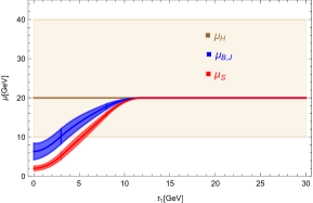
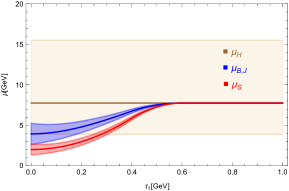
Figure 2: Profile functions for μH,μB,J,subscript𝜇𝐻subscript𝜇𝐵𝐽\mu_{H},\mu_{B,J}, and μSsubscript𝜇𝑆\mu_{S}, along with their scale variation bands, for the τ1subscript𝜏1\tau_{1} (left panel) and τ1asubscript𝜏1𝑎\tau_{1a} (right panel) observables. The plots correspond to the choices QH=PJT=20.0subscript𝑄𝐻subscript𝑃subscript𝐽𝑇20.0Q_{H}=P_{J_{T}}=20.0 GeV and QH=Q2=60.0subscript𝑄𝐻superscript𝑄260.0Q_{H}=\sqrt{Q^{2}}=\sqrt{60.0} GeV for the τ1subscript𝜏1\tau_{1} and τ1asubscript𝜏1𝑎\tau_{1a} distributions, respectively. The scale variation bands are generated using the scale variations in Eq. (III.4).

Fig. 2 shows the profile functions for μH,μB,J,subscript𝜇𝐻subscript𝜇𝐵𝐽\mu_{H},\mu_{B,J}, and μSsubscript𝜇𝑆\mu_{S}, along with their corresponding scale variations as described above, for the τ1subscript𝜏1\tau_{1} (left panel) and τ1asubscript𝜏1𝑎\tau_{1a} (right panel). These profile function curves are for the choice μH=PJT=20.0subscript𝜇𝐻subscript𝑃subscript𝐽𝑇20.0\mu_{H}=P_{J_{T}}=20.0 GeV and μH=Q2=60.0subscript𝜇𝐻superscript𝑄260.0\mu_{H}=\sqrt{Q^{2}}=\sqrt{60.0} GeV for the τ1subscript𝜏1\tau_{1} and τ1asubscript𝜏1𝑎\tau_{1a} distributions, respectively. We see that the profile functions smoothly connect the resummation and fixed order regions. i.e. the μH,μB,J,subscript𝜇𝐻subscript𝜇𝐵𝐽\mu_{H},\mu_{B,J}, and μSsubscript𝜇𝑆\mu_{S} scales have the appropriate scalings in the resummation region and smoothly converge in the fixed order region.

We note that in the subsequent section on numerical results, for the τ1subscript𝜏1\tau_{1} distribution we choose QH=ξ2subscript𝑄𝐻superscript𝜉2Q_{H}=\sqrt{\xi^{2}} in Eq. (III.4), instead of QH=PJTsubscript𝑄𝐻subscript𝑃subscript𝐽𝑇Q_{H}=P_{J_{T}}, corresponding to minimizing logarithms of the exact argument appearing in the hard function in the resummation region, as seen in Eqs. (26) and (27). This choice still has the same scaling ξ2PJTsimilar-tosuperscript𝜉2subscript𝑃subscript𝐽𝑇\sqrt{\xi^{2}}\sim P_{J_{T}} as seen in Eqs. (50) and (53). We have also checked that both choices give consistent results.

IV Numerical Results

In this section, we provide numerical results up to the N3LL+NNLO level of accuracy. For the τ1subscript𝜏1\tau_{1}-spectrum we provide numerical results for the following choice of kinematics:

τ1:s=90.0GeV,PJT=[20.0GeV,30.0GeV],yJ=[2.5,2.5],\displaystyle\tau_{1}:\qquad\sqrt{s}=90.0\>{\rm GeV},\qquad P_{J_{T}}=[20.0\>{\rm GeV},30.0\>{\rm GeV}],\qquad y_{J}=[-2.5,2.5], (46)

corresponding to typical EIC kinematics. For the τ1asubscript𝜏1𝑎\tau_{1a}-spectrum we choose:

τ1a:s=319.0GeV,Q2=[60.0GeV2,80.0GeV2],y=[0.2,0.6],\displaystyle\tau_{1a}:\qquad\sqrt{s}=319.0\>{\rm GeV},\qquad Q^{2}=[60.0\>{\rm GeV}^{2},80.0\>{\rm GeV}^{2}],\qquad y=[0.2,0.6], (47)

corresponding to typical HERA kinematics.

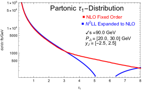
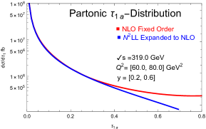
First, we provide results at the partonic level, ignoring final state hadronization effects. In Fig. 3, we show the dσresumFO𝑑superscriptsubscript𝜎resumFOd\sigma_{\rm resum}^{\rm FO} (blue) and dσFO𝑑superscript𝜎FOd\sigma^{\rm FO} (red) contributions to the N2LL+NLO matched cross section in Eq. (18). The left and right panels correspond to the τ1subscript𝜏1\tau_{1} and τ1asubscript𝜏1𝑎\tau_{1a} distributions, respectively. As expected, in the small τ1subscript𝜏1\tau_{1} (τ1asubscript𝜏1𝑎\tau_{1a}) region where the fixed order result is dominated by the singular terms, dσFO𝑑superscript𝜎FOd\sigma^{\rm FO} at NLO approaches dσresumFO𝑑superscriptsubscript𝜎resumFOd\sigma_{\rm resum}^{\rm FO} expanded to NLO. In the region around τ15greater-than-or-equivalent-tosubscript𝜏15\tau_{1}\gtrsim 5 GeV (τ1a0.7greater-than-or-equivalent-tosubscript𝜏1𝑎0.7\tau_{1a}\gtrsim 0.7), the contribution of the singular terms to the NLO result goes negative, and the non-singular terms in dσFO𝑑superscript𝜎FOd\sigma^{\rm FO} at NLO become important.

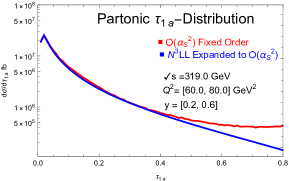
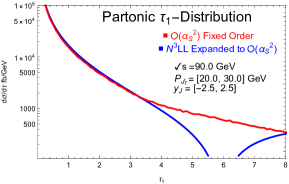
Similarly, in Fig. 4 we show the dσresumFO𝑑superscriptsubscript𝜎resumFOd\sigma_{\rm resum}^{\rm FO} (blue) and dσFO𝑑superscript𝜎FOd\sigma^{\rm FO} (red) contributions to the N3LL+𝒪(αs2)𝒪superscriptsubscript𝛼𝑠2{\cal O}(\alpha_{s}^{2}) matched cross section in Eq. (18). Once again, as expected, we see that in the small τ1subscript𝜏1\tau_{1} (τ1asubscript𝜏1𝑎\tau_{1a}) region, dσFO𝑑superscript𝜎FOd\sigma^{\rm FO} at 𝒪(αs2)𝒪superscriptsubscript𝛼𝑠2{\cal O}(\alpha_{s}^{2}) approaches dσresumFO𝑑superscriptsubscript𝜎resumFOd\sigma_{\rm resum}^{\rm FO} expanded to 𝒪(αs2)𝒪superscriptsubscript𝛼𝑠2{\cal O}(\alpha_{s}^{2}). Once again, in the region around τ15greater-than-or-equivalent-tosubscript𝜏15\tau_{1}\gtrsim 5 GeV ( τ1a0.7greater-than-or-equivalent-tosubscript𝜏1𝑎0.7\tau_{1a}\gtrsim 0.7), the contribution of the non-singular terms in dσFO𝑑superscript𝜎FOd\sigma^{\rm FO} at 𝒪(αs2)𝒪superscriptsubscript𝛼𝑠2{\cal O}(\alpha_{s}^{2}) become important.

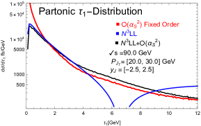
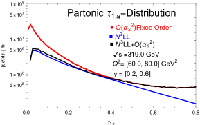
In Fig. 5, we show dσFO𝑑superscript𝜎FOd\sigma^{\rm FO} at 𝒪(αs2)𝒪superscriptsubscript𝛼𝑠2{\cal O}(\alpha_{s}^{2}) (red) , dσresum.𝑑subscript𝜎resumd\sigma_{\rm resum.} at N3LL (blue), and the matched result, dσ𝑑𝜎d\sigma, at N3LL+𝒪(αs2)𝒪superscriptsubscript𝛼𝑠2{\cal O}(\alpha_{s}^{2}) (black) for the τ1subscript𝜏1\tau_{1} (left panel) and τ1asubscript𝜏1𝑎\tau_{1a} (right panel) distributions. We note that as expected, the matched distribution approaches the resummation result for small τ1subscript𝜏1\tau_{1} or τ1asubscript𝜏1𝑎\tau_{1a} and the fixed order result for large τ1subscript𝜏1\tau_{1} or τ1asubscript𝜏1𝑎\tau_{1a}.

Refer to caption
Refer to caption
Figure 3: Comparison of the resummation expanded singular contribution (blue curve) and the full NLO prediction from NLOJET++ (red curve) for both τ1subscript𝜏1\tau_{1} (left panel) and τ1asubscript𝜏1𝑎\tau_{1a} (right panel). Good agreement is observed, validating our computational setup.

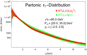
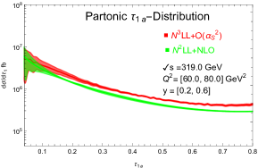
In Fig. 6, we show the matched τ1subscript𝜏1\tau_{1} (left panel) and τ1asubscript𝜏1𝑎\tau_{1a} (right panel) distributions, corresponding to Eq. (18), along with their scale variation bands at the N2LL+NLO (green) and N3LL+𝒪(αs2)𝒪superscriptsubscript𝛼𝑠2{\cal O}(\alpha_{s}^{2}) (red) levels of accuracy.

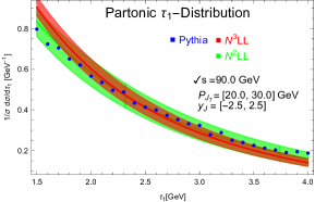
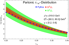
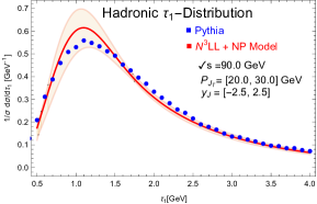
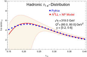
In Fig. 7, we show that the τ1subscript𝜏1\tau_{1} (left panel) and τ1asubscript𝜏1𝑎\tau_{1a} (right panel) distributions in the resummation region, normalized to the central curve over the displayed region. We see good convergence in going from the N2LL to N3LL resummation curves. We also display the corresponding results of Pythia8 Bierlich:2022pfr simulations (blue dots) and find relatively good agreement.
Refer to caption
Refer to caption
Figure 4: Comparison of the resummation expanded singular contribution (blue curve) and the full prediction from NLOJET++ up to 𝒪(αs2)𝒪superscriptsubscript𝛼𝑠2{\cal O}(\alpha_{s}^{2}) (red curve) for both τ1subscript𝜏1\tau_{1} (left panel) and τ1asubscript𝜏1𝑎\tau_{1a} (right panel). Good agreement is observed, validating our computational setup.
Refer to caption
Refer to caption
Figure 5: As seen in the left (right) panel, for the τ1subscript𝜏1\tau_{1} (τ1asubscript𝜏1𝑎\tau_{1a}) distributions of Eq. (18), the N3LL+αs2superscriptsubscript𝛼𝑠2\alpha_{s}^{2} (black) matched distribution approaches the N3LL (blue) and 𝒪(αs2)𝒪superscriptsubscript𝛼𝑠2{\cal O}(\alpha_{s}^{2}) (red) results in the τ1PJTmuch-less-thansubscript𝜏1subscript𝑃subscript𝐽𝑇\tau_{1}\ll P_{J_{T}} (τ1a1much-less-thansubscript𝜏1𝑎1\tau_{1a}\ll 1) and τ1aPJTsimilar-tosubscript𝜏1𝑎subscript𝑃subscript𝐽𝑇\tau_{1a}\sim P_{J_{T}} (τ1a1similar-tosubscript𝜏1𝑎1\tau_{1a}\sim 1) regions, respectively.
Refer to caption
Refer to caption
Figure 6: Partonic resummed results for τ1subscript𝜏1\tau_{1} (left panel) and τ1asubscript𝜏1𝑎\tau_{1a} (right panel) at the N3LL+𝒪(αs2)𝒪superscriptsubscript𝛼𝑠2{\cal O}(\alpha_{s}^{2}) (red) and N2LL+NLO (green) levels of accuracy.
Refer to caption
Refer to caption
Figure 7: The τ1subscript𝜏1\tau_{1} (left panel) and τ1asubscript𝜏1𝑎\tau_{1a} (right panel) distributions with scale variations normalized to the central curve over the displayed range, at the N2LL (green) and N3LL (red) level of accuracy.
Refer to caption
Refer to caption
Figure 8: The τ1subscript𝜏1\tau_{1} (left panel) and τ1asubscript𝜏1𝑎\tau_{1a} (right panel) N3LL+Soft Function Model distributions with scale variations (tan band) normalized to the central curve (red) over the displayed range, compared to Pythia data (blue dots).

Finally, we perform a preliminary study of hadronization effects using a soft function model, following Eqs. (30), (31), and (32). In Fig. 8, we show the τ1subscript𝜏1\tau_{1} (left panel) and τ1asubscript𝜏1𝑎\tau_{1a} (right panel) distributions (red curve), along with their scale variation bands (tan color), in the resummation region where non-perturbative effects are important (see Table 1). The results are normalized to the central curve in the displayed region. The results are generated through a convolution of a non-perturbative soft function model with the perturbative N3LL resummation curve as in Eq. (30). We also show the results from Pythia8 (blue dots) with hadronization turned on. As mentioned earlier below Eq. (32), in general one expects different non-perturbtive effects (soft function models) for the τ1subscript𝜏1\tau_{1} and τ1asubscript𝜏1𝑎\tau_{1a} distributions due to the correspondingly different measurement functions at the operator level. For the τ1subscript𝜏1\tau_{1} distribution, the results where generated using model parameters with values a=1.0,b=0.45,formulae-sequence𝑎1.0𝑏0.45a=1.0,b=0.45, and Λ=0.5Λ0.5\Lambda=0.5 GeV in Eq. (32). For the τ1asubscript𝜏1𝑎\tau_{1a} distribution, we used a=1.0,b=0.75,formulae-sequence𝑎1.0𝑏0.75a=1.0,b=0.75, and Λ=0.5Λ0.5\Lambda=0.5 GeV. We see that for these choices of the soft function model parameters there is good agreement between the Pythia8 results and the theory predictions. We note that the scale variation band for the τ1asubscript𝜏1𝑎\tau_{1a} distribution (right panel) in Fig. 8 is relatively large because of the choice of a relatively small hard scale, μH2=Q2=[60.0,80]superscriptsubscript𝜇𝐻2superscript𝑄260.080\mu_{H}^{2}=Q^{2}=[60.0,80] GeV2. The hard scale variation around this small central value leads to a relatively large variation in the value of the strong coupling. We have checked that at larger Q2superscript𝑄2Q^{2} the scale variation is much smaller and similar to what is seen for τ1subscript𝜏1\tau_{1}, which is evaluated and varied around a larger hard scale μHPJT=20.0similar-tosubscript𝜇𝐻subscript𝑃subscript𝐽𝑇20.0\mu_{H}\sim P_{J_{T}}=20.0 GeV.

We note that these results in the non-perturbative region are only meant to demonstrate that one can easily find an appropriate soft function model to describe the Pythia8 hadronization effects. We leave a more detailed and rigorous best-fit extraction of the soft function model parameters for future work. Relatedly, there can also be important renormalon effects in the soft function Hoang:2007vb ; Abbate:2010xh that can affect the extraction of the soft function model parameters, and is also left for future work.

The numerical results given in this section provide a benchmark for further analyses using simulations for the proposed EIC and data collected at HERA.

V Conclusion

We have provided results for the 1-Jettiness spectrum in Deep Inelastic Scattering (DIS), up to the N3LL+𝒪(αs2)𝒪superscriptsubscript𝛼𝑠2{\cal O}(\alpha_{s}^{2}) level of accuracy. In particular, we considered two types of 1-Jettiness distributions, dσ[τ1,PJT,yJ]𝑑𝜎subscript𝜏1subscript𝑃subscript𝐽𝑇subscript𝑦𝐽d\sigma\left[\tau_{1},P_{J_{T}},y_{J}\right] and dσ[τ1a,Q2,y]𝑑𝜎subscript𝜏1𝑎superscript𝑄2𝑦d\sigma\left[\tau_{1a},Q^{2},y\right], where τ1subscript𝜏1\tau_{1} and τ1asubscript𝜏1𝑎\tau_{1a} denote two different definitions of the 1-jettiness global event shape. We also discussed the differences and complementarity between these two types of 1-jettiness distributions. In the resummation region, corresponding to energetic final state radiation being closely aligned with either the beam or leading jet directions, a factorization framework is used and corresponding analytic formulae are provided, up to the N3LL level of accuracy. In the region of very small 1-Jettiness, where the distribution becomes sensitive to the non-perturbative soft radiation throughout the event, a phenomenological model is employed to describe non-perturbative effects. In the fixed order region, corresponding to energetic final state radiation at wide angles from the beam or leading jet directions, fixed order perturbative QCD is appropriate. Fixed order results up to 𝒪(αs2)𝒪superscriptsubscript𝛼𝑠2{\cal O}(\alpha_{s}^{2}) are implemented using NLOJET++ Nagy:2005gn program and smoothly matched with the factorization framework in the resummation region. We also provided a comparison of the theory predictions with Pythia8 simulation results, including a preliminary study of hadronization effects. These results allow for further detailed phenomenological studies of nuclear structure, nuclear medium effects, and a precision extraction of the strong coupling. The results presented here can be adapted to analyses with HERA data, ongoing EIC simulation studies, and eventual real data from the EIC.

Acknowledgement

H. C. and X. L. are supported by the Natural Science Foundation of China under contract No. 12175016. Z.K. is supported by the National Science Foundation under grant No. PHY-1945471. S.M. thanks UNG for support through the 2022 Presidential Summer Incentive Award program.

Appendix A Relationship Between τ1subscript𝜏1\tau_{1} and τ1asubscript𝜏1𝑎\tau_{1a} in the Resummation Region

In this section, we derive the relationship in Eq. (III.1) connecting dσresum[τ1a,Q2,y]𝑑subscript𝜎resumsubscript𝜏1𝑎superscript𝑄2𝑦d\sigma_{\rm resum}\left[\tau_{1a},Q^{2},y\right] and dσresum[τ1,PJT,yJ]𝑑subscript𝜎resumsubscript𝜏1subscript𝑃subscript𝐽𝑇subscript𝑦𝐽d\sigma_{\rm resum}\left[\tau_{1},P_{J_{T}},y_{J}\right]. In the resummation region (τ1PJTorτ1a1much-less-thansubscript𝜏1subscript𝑃subscript𝐽𝑇orsubscript𝜏1𝑎much-less-than1\tau_{1}\ll P_{J_{T}}\>\text{or}\>\>\>\>\tau_{1a}\ll 1), up to power suppressed corrections, one can identify the 1-jettiness jet momentum as

PJ=q+xP,subscript𝑃𝐽𝑞𝑥𝑃\displaystyle P_{J}=q+xP, (48)

corresponding to the momentum of the quark or anti-quark emerging from the hard parton-level scattering. Thus, the partonic Mandelstam variables can be expressed as

s^=(k+xP)2,t^=(PJxP)2=q2=Q2,u^=(kPJ)2,formulae-sequenceformulae-sequence^𝑠superscript𝑘𝑥𝑃2^𝑡superscriptsubscript𝑃𝐽𝑥𝑃2superscript𝑞2superscript𝑄2^𝑢superscript𝑘subscript𝑃𝐽2\displaystyle\hat{s}=(k+xP)^{2},\qquad\hat{t}=(P_{J}-xP)^{2}=q^{2}=-Q^{2},\qquad\hat{u}=(k-P_{J})^{2}, (49)

which can in turn be expressed in terms of s=(k+P)2𝑠superscript𝑘𝑃2s=(k+P)^{2}, PJTsubscript𝑃subscript𝐽𝑇P_{J_{T}}, and yJsubscript𝑦𝐽y_{J} as

s^=xs,t^=Q2=xsPJTeyJ,u^=sPJTeyJ,formulae-sequenceformulae-sequence^𝑠𝑥𝑠^𝑡superscript𝑄2𝑥𝑠subscript𝑃subscript𝐽𝑇superscript𝑒subscript𝑦𝐽^𝑢𝑠subscript𝑃subscript𝐽𝑇superscript𝑒subscript𝑦𝐽\displaystyle\hat{s}=xs,\qquad\hat{t}=-Q^{2}=-x\sqrt{s}P_{J_{T}}e^{-y_{J}},\qquad\hat{u}=-\sqrt{s}P_{J_{T}}e^{y_{J}}, (50)

where we have ignored terms proportional to the electron or parton masses. Furthermore, in this limit of massless electrons and partons, the partonic Mandelstam variables satisfy the constraint

s^+t^+u^=0,^𝑠^𝑡^𝑢0\displaystyle\hat{s}+\hat{t}+\hat{u}=0, (51)

from which we can solve for the momentum fraction of the struck quark or anti-quark to get the result

x𝑥\displaystyle x =\displaystyle= PJTeyJsPJTeyJ.subscript𝑃subscript𝐽𝑇superscript𝑒subscript𝑦𝐽𝑠subscript𝑃subscript𝐽𝑇superscript𝑒subscript𝑦𝐽\displaystyle\frac{P_{J_{T}}\>e^{y_{J}}}{\sqrt{s}-P_{J_{T}}\>e^{-y_{J}}}. (52)

Using this result for x𝑥x in Eq. (50), we can write Q2superscript𝑄2Q^{2} and the inelasticity parameter y=Pq/Pk=Q2/(xs)𝑦𝑃𝑞𝑃𝑘superscript𝑄2𝑥𝑠y=P\cdot q/P\cdot k=Q^{2}/(xs) as

Q2=PJT21PJTseyJ,y=PJTseyJ.formulae-sequencesuperscript𝑄2superscriptsubscript𝑃subscript𝐽𝑇21subscript𝑃subscript𝐽𝑇𝑠superscript𝑒subscript𝑦𝐽𝑦subscript𝑃subscript𝐽𝑇𝑠superscript𝑒subscript𝑦𝐽\displaystyle Q^{2}=\frac{P_{J_{T}}^{2}}{1-\frac{P_{J_{T}}}{\sqrt{s}}\>e^{-y_{J}}},\qquad y=\frac{P_{J_{T}}}{\sqrt{s}}\>e^{-y_{J}}. (53)

Note that ξ2superscript𝜉2\xi^{2} in Eq. (27) is equivalent to Q2superscript𝑄2Q^{2} expressed in terms of s,PJT,𝑠subscript𝑃subscript𝐽𝑇\sqrt{s},P_{J_{T}}, and yJsubscript𝑦𝐽y_{J}, as above in Eq. (53). Inverting these equations, we can write PJTsubscript𝑃subscript𝐽𝑇P_{J_{T}} and yJsubscript𝑦𝐽y_{J} in terms of Q2superscript𝑄2Q^{2} and y𝑦y as

PJT=Q2(1y),yJ=12lnQ2(1y)y2s,formulae-sequencesubscript𝑃subscript𝐽𝑇superscript𝑄21𝑦subscript𝑦𝐽12superscript𝑄21𝑦superscript𝑦2𝑠\displaystyle P_{J_{T}}=\sqrt{Q^{2}(1-y)},\qquad y_{J}=\frac{1}{2}\ln\frac{Q^{2}(1-y)}{y^{2}s}, (54)

from which we obtain the Jacobian for the change of variables from (PJT,yJ)subscript𝑃subscript𝐽𝑇subscript𝑦𝐽(P_{J_{T}},y_{J}) to (Q2,y)superscript𝑄2𝑦(Q^{2},y):

dQ2dy𝑑superscript𝑄2𝑑𝑦\displaystyle dQ^{2}\>dy =\displaystyle= 2yQ21ydPJTdyJ.2𝑦superscript𝑄21𝑦𝑑subscript𝑃subscript𝐽𝑇𝑑subscript𝑦𝐽\displaystyle 2y\>\sqrt{\frac{Q^{2}}{1-y}}\>dP_{J_{T}}\>dy_{J}. (55)

From the definitions of τ1subscript𝜏1\tau_{1} and τ1asubscript𝜏1𝑎\tau_{1a} in Eqs. (4) and (7), respectively, one can show that they are related to each other as

τ1a=1Q2τ1(QBQ2,QJQ2),dτ1a=1Q2dτ1.formulae-sequencesubscript𝜏1𝑎1superscript𝑄2subscript𝜏1formulae-sequencesubscript𝑄𝐵superscript𝑄2subscript𝑄𝐽superscript𝑄2𝑑subscript𝜏1𝑎1superscript𝑄2𝑑subscript𝜏1\displaystyle\tau_{1a}=\frac{1}{\sqrt{Q^{2}}}\>\tau_{1}(Q_{B}\to\sqrt{Q^{2}},Q_{J}\to\sqrt{Q^{2}}),\qquad d\tau_{1a}=\frac{1}{\sqrt{Q^{2}}}\>d\tau_{1}. (56)

Putting together Eqs. (55) and (56), we get

dτ1adQ2dy𝑑subscript𝜏1𝑎𝑑superscript𝑄2𝑑𝑦\displaystyle d\tau_{1a}dQ^{2}\>dy =\displaystyle= 2y1ydτ1dPJTdyJ,2𝑦1𝑦𝑑subscript𝜏1𝑑subscript𝑃subscript𝐽𝑇𝑑subscript𝑦𝐽\displaystyle\frac{2y}{\sqrt{1-y}}\>d\tau_{1}dP_{J_{T}}dy_{J}, (57)

which along with Eq. (54) gives the final result of Eq. (III.1).

Appendix B Useful Identities

The plus-distributions, n(z)subscript𝑛𝑧{\cal L}_{n}(z), for n0𝑛0n\geq 0, are defined as

n(z)subscript𝑛𝑧\displaystyle{\cal L}_{n}(z) \displaystyle\equiv [θ(z)lnnzz]+=limβ0[θ(zβ)lnnzz+δ(zβ)lnn+1βn+1],subscriptdelimited-[]𝜃𝑧superscript𝑛𝑧𝑧subscript𝛽0delimited-[]𝜃𝑧𝛽superscript𝑛𝑧𝑧𝛿𝑧𝛽superscript𝑛1𝛽𝑛1\displaystyle\left[\frac{\theta(z)\ln^{n}z}{z}\right]_{+}=\lim_{\beta\to 0}\left[\frac{\theta(z-\beta)\ln^{n}z}{z}+\delta(z-\beta)\frac{\ln^{n+1}\beta}{n+1}\right], (58)

for any dimensionless variable z𝑧z. Using this definition, for α𝛼\alpha\in\mathbb{R} and α>0𝛼0\alpha>0, via explicit calculation the Laplace transform of n(z)subscript𝑛𝑧{\cal L}_{n}(z) is given by:

0𝑑zeαzn(z)=1n+1k=0n+1(1)n+1k(n+1k)(lnα)n+1k0𝑑ueu(lnu)k.superscriptsubscript0differential-d𝑧superscript𝑒𝛼𝑧subscript𝑛𝑧1𝑛1superscriptsubscript𝑘0𝑛1superscript1𝑛1𝑘binomial𝑛1𝑘superscript𝛼𝑛1𝑘superscriptsubscript0differential-d𝑢superscript𝑒𝑢superscript𝑢𝑘\displaystyle\int_{0}^{\infty}dz\>e^{-\alpha z}{\cal L}_{n}(z)=\frac{1}{n+1}\sum_{k=0}^{n+1}(-1)^{n+1-k}\binom{n+1}{k}\left(\ln\alpha\right)^{n+1-k}\int_{0}^{\infty}du\>e^{-u}\left(\ln u\right)^{k}. (59)

This result can be analytically continued to αiy𝛼𝑖𝑦\alpha\to iy, for y𝑦y\in\mathbb{R}, to get the Fourier transform of the n(z)subscript𝑛𝑧{\cal L}_{n}(z) distributions, which are useful for computing the Fourier transforms of the beam, jet, and soft functions in Eq. (III.3). Explicit results for the cases of n=0,1,2,𝑛012n=0,1,2, and 333 are:

0𝑑zeiyz0(z)superscriptsubscript0differential-d𝑧superscript𝑒𝑖𝑦𝑧subscript0𝑧\displaystyle\int_{0}^{\infty}dz\>e^{-iyz}{\cal L}_{0}(z) =\displaystyle= L,𝐿\displaystyle-L,
0𝑑zeiyz1(z)superscriptsubscript0differential-d𝑧superscript𝑒𝑖𝑦𝑧subscript1𝑧\displaystyle\int_{0}^{\infty}dz\>e^{-iyz}{\cal L}_{1}(z) =\displaystyle= 12L2+π212,12superscript𝐿2superscript𝜋212\displaystyle\frac{1}{2}L^{2}+\frac{\pi^{2}}{12}, (60)
0𝑑zeiyz2(z)superscriptsubscript0differential-d𝑧superscript𝑒𝑖𝑦𝑧subscript2𝑧\displaystyle\int_{0}^{\infty}dz\>e^{-iyz}{\cal L}_{2}(z) =\displaystyle= 13L3π26L23ζ3,13superscript𝐿3superscript𝜋26𝐿23subscript𝜁3\displaystyle-\frac{1}{3}L^{3}-\frac{\pi^{2}}{6}L-\frac{2}{3}\zeta_{3},
0𝑑zeiyz3(z)superscriptsubscript0differential-d𝑧superscript𝑒𝑖𝑦𝑧subscript3𝑧\displaystyle\int_{0}^{\infty}dz\>e^{-iyz}{\cal L}_{3}(z) =\displaystyle= 14L4+π24L2+2ζ3L+3π480,14superscript𝐿4superscript𝜋24superscript𝐿22subscript𝜁3𝐿3superscript𝜋480\displaystyle\frac{1}{4}L^{4}+\frac{\pi^{2}}{4}L^{2}+2\zeta_{3}L+\frac{3\pi^{4}}{80},

where we have defined

Lln(iyeγE),𝐿𝑖𝑦superscript𝑒subscript𝛾𝐸\displaystyle L\equiv\ln(iye^{\gamma_{E}}), (61)

and Euler’s constant, γEsubscript𝛾𝐸\gamma_{E}, can be expressed as the definite integral:

γE=0𝑑ueulnu,subscript𝛾𝐸superscriptsubscript0differential-d𝑢superscript𝑒𝑢𝑢\displaystyle\gamma_{E}=-\int_{0}^{\infty}du\>e^{-u}\ln u, (62)

and ζssubscript𝜁𝑠\zeta_{s} is the Riemann zeta function defined by

ζs=n=01ns=1Γ(s)0xs1ex1𝑑x,subscript𝜁𝑠superscriptsubscript𝑛01superscript𝑛𝑠1Γ𝑠superscriptsubscript0superscript𝑥𝑠1superscript𝑒𝑥1differential-d𝑥\displaystyle\zeta_{s}=\sum_{n=0}^{\infty}\frac{1}{n^{s}}=\frac{1}{\Gamma(s)}\int_{0}^{\infty}\frac{x^{s-1}}{e^{x}-1}dx, (63)

for Re(s)>1𝑠1(s)>1 and by analytic continuation elsewhere. Numerically, γE0.5772similar-to-or-equalssubscript𝛾𝐸0.5772\gamma_{E}\simeq 0.5772 and ζ31.202similar-to-or-equalssubscript𝜁31.202\zeta_{3}\simeq 1.202. The results in Eq. (B) follow from using the identities:

0𝑑ueuln2usuperscriptsubscript0differential-d𝑢superscript𝑒𝑢superscript2𝑢\displaystyle\int_{0}^{\infty}du\>e^{-u}\ln^{2}u =\displaystyle= γE2+π26,superscriptsubscript𝛾𝐸2superscript𝜋26\displaystyle\gamma_{E}^{2}+\frac{\pi^{2}}{6}, (64)
0𝑑ueuln3usuperscriptsubscript0differential-d𝑢superscript𝑒𝑢superscript3𝑢\displaystyle\int_{0}^{\infty}du\>e^{-u}\ln^{3}u =\displaystyle= γE3γEπ222ζ3,superscriptsubscript𝛾𝐸3subscript𝛾𝐸superscript𝜋222subscript𝜁3\displaystyle-\gamma_{E}^{3}-\gamma_{E}\frac{\pi^{2}}{2}-2\>\zeta_{3},
0𝑑ueuln4usuperscriptsubscript0differential-d𝑢superscript𝑒𝑢superscript4𝑢\displaystyle\int_{0}^{\infty}du\>e^{-u}\ln^{4}u =\displaystyle= γE4+γE2π2+8γEζ3+3π420\displaystyle\gamma_{E}^{4}+\gamma_{E}^{2}\pi^{2}+8\>\gamma_{E}\>\zeta_{3}+\frac{3\pi^{4}}{20}\cdot

Another useful plus-distribution is:

[θ(x)x1+ω]+subscriptdelimited-[]𝜃𝑥superscript𝑥1𝜔\displaystyle\left[\frac{\theta(x)}{x^{1+\omega}}\right]_{+} =\displaystyle= limβ0[θ(xβ)x1+ωδ(xβ)βωω],subscript𝛽0delimited-[]𝜃𝑥𝛽superscript𝑥1𝜔𝛿𝑥𝛽superscript𝛽𝜔𝜔\displaystyle\lim_{\beta\to 0}\left[\frac{\theta(x-\beta)}{x^{1+\omega}}-\delta(x-\beta)\frac{\beta^{-\omega}}{\omega}\right], (65)

which can be used to show:

(iyeγE)ω=eωγEΓ(ω)𝑑zeizy[θ(z)z1+ω]+.superscript𝑖𝑦superscript𝑒subscript𝛾𝐸𝜔superscript𝑒𝜔subscript𝛾𝐸Γ𝜔differential-d𝑧superscript𝑒𝑖𝑧𝑦subscriptdelimited-[]𝜃𝑧superscript𝑧1𝜔\displaystyle\big{(}iye^{\gamma_{E}}\big{)}^{\omega}=\frac{e^{\omega\gamma_{E}}}{\Gamma(-\omega)}\int dz\>e^{-izy}\>\left[\frac{\theta(z)}{z^{1+\omega}}\right]_{+}. (66)

Appendix C Fixed Order Results

In this section, we collect results for the hard, beam, jet, and soft functions up to the NNLO level of accuracy in perturbation theory. These results are needed to carry out resummation of the τ1subscript𝜏1\tau_{1}- and τ1asubscript𝜏1𝑎\tau_{1a}-distributions at the N3LL level of accuracy, using Eqs. (III.3) and (III.1), respectively.

C.1 Hard Function

The hard function is given by

H(Q2,μ)𝐻superscript𝑄2𝜇\displaystyle H(Q^{2},\mu) =\displaystyle= |C(Q2,μ)|2,superscript𝐶superscript𝑄2𝜇2\displaystyle|C(Q^{2},\mu)|^{2}, (67)

where C(Q2,μ)𝐶superscript𝑄2𝜇C(Q^{2},\mu) is the Wilson coefficient that arises from matching the QCD current operators in Eq. (12) onto the corresponding SCET current operators. The fixed order perturbvative expansion of the C(Q2,μ)𝐶superscript𝑄2𝜇C(Q^{2},\mu) Wilson coefficient is expressed as:

C(Q2,μ)=n=0[αs(μ)4π]nC(n)𝐶superscript𝑄2𝜇superscriptsubscript𝑛0superscriptdelimited-[]subscript𝛼𝑠𝜇4𝜋𝑛superscript𝐶𝑛\displaystyle C(Q^{2},\mu)=\sum_{n=0}^{\infty}\left[\frac{\alpha_{s}(\mu)}{4\pi}\right]^{n}C^{(n)} (68)

The result for the Wilson coefficient is known up to NNLO Idilbi_2006 ; Becher:2006mr :

C(0)superscript𝐶0\displaystyle C^{(0)} =\displaystyle= 1,1\displaystyle 1,
C(1)superscript𝐶1\displaystyle C^{(1)} =\displaystyle= CF(L2+3L8+π26),subscript𝐶𝐹superscript𝐿23𝐿8superscript𝜋26\displaystyle C_{F}\big{(}-L^{2}+3L-8+\frac{\pi^{2}}{6}\big{)},\, (69)
C(2)superscript𝐶2\displaystyle C^{(2)} =\displaystyle= CF(CFHF+CAHA+TFnfHf),subscript𝐶𝐹subscript𝐶𝐹subscript𝐻𝐹subscript𝐶𝐴subscript𝐻𝐴subscript𝑇𝐹subscript𝑛𝑓subscript𝐻𝑓\displaystyle C_{F}\big{(}C_{F}H_{F}+C_{A}H_{A}+T_{F}n_{f}H_{f}\big{)},

where L=lnQ2μ2𝐿superscript𝑄2superscript𝜇2L=\ln\frac{Q^{2}}{\mu^{2}} and the HF,A,fsubscript𝐻𝐹𝐴𝑓H_{F,A,f} coefficients are defined as

HFsubscript𝐻𝐹\displaystyle H_{F} =\displaystyle= L423L3+(252π26)L2+(4523π22+24ζ3)L+2558+7π2283π436030ζ3,superscript𝐿423superscript𝐿3252superscript𝜋26superscript𝐿24523superscript𝜋2224subscript𝜁3𝐿25587superscript𝜋2283superscript𝜋436030subscript𝜁3\displaystyle\frac{L^{4}}{2}-3L^{3}+\left(\frac{25}{2}-\frac{\pi^{2}}{6}\right)L^{2}+\left(-\frac{45}{2}-\frac{3\pi^{2}}{2}+24\zeta_{3}\right)L+\frac{255}{8}+\frac{7\pi^{2}}{2}-\frac{83\pi^{4}}{360}-30\zeta_{3},
HAsubscript𝐻𝐴\displaystyle H_{A} =\displaystyle= 119L3+(23318+π23)L2+(254554+11π2926ζ3)L51157648337π2108+11π445+3139ζ3,119superscript𝐿323318superscript𝜋23superscript𝐿225455411superscript𝜋2926subscript𝜁3𝐿51157648337superscript𝜋210811superscript𝜋4453139subscript𝜁3\displaystyle\frac{11}{9}L^{3}+\left(-\frac{233}{18}+\frac{\pi^{2}}{3}\right)L^{2}+\left(\frac{2545}{54}+\frac{11\pi^{2}}{9}-26\zeta_{3}\right)L-\frac{51157}{648}-\frac{337\pi^{2}}{108}+\frac{11\pi^{4}}{45}+\frac{313}{9}\zeta_{3},
Hfsubscript𝐻𝑓\displaystyle H_{f} =\displaystyle= 49L3+389L2+(418274π29)L+4085162+23π227+49ζ349superscript𝐿3389superscript𝐿2418274superscript𝜋29𝐿408516223superscript𝜋22749subscript𝜁3\displaystyle-\frac{4}{9}L^{3}+\frac{38}{9}L^{2}+\left(-\frac{418}{27}-\frac{4\pi^{2}}{9}\right)L+\frac{4085}{162}+\frac{23\pi^{2}}{27}+\frac{4}{9}\zeta_{3} (70)

The hard function can be can be correspondingly expressed as

H(Q2,μ)𝐻superscript𝑄2𝜇\displaystyle H(Q^{2},\mu) =\displaystyle= |C(Q2,μ)|2=n=0[αs(μ)4π]nH(n),superscript𝐶superscript𝑄2𝜇2superscriptsubscript𝑛0superscriptdelimited-[]subscript𝛼𝑠𝜇4𝜋𝑛superscript𝐻𝑛\displaystyle|C(Q^{2},\mu)|^{2}=\sum_{n=0}^{\infty}\left[\frac{\alpha_{s}(\mu)}{4\pi}\right]^{n}H^{(n)}, (71)

where the coefficients H(n)superscript𝐻𝑛H^{(n)}, expressed in terms of the C(n)superscript𝐶𝑛C^{(n)} coefficients, up to NNLO are given by:

H(0)superscript𝐻0\displaystyle H^{(0)} =\displaystyle= 1,1\displaystyle 1,
H(1)superscript𝐻1\displaystyle H^{(1)} =\displaystyle= 2C(1)2superscript𝐶1\displaystyle 2C^{(1)}
H(2)superscript𝐻2\displaystyle H^{(2)} =\displaystyle= 2C(2)+(C(1))22superscript𝐶2superscriptsuperscript𝐶12\displaystyle 2C^{(2)}+(C^{(1)})^{2} (72)

C.2 Soft Function

The fixed order perturbative expansion of the soft function in momentum space can be expressed as:

S(τ1,μS)𝑆subscript𝜏1subscript𝜇𝑆\displaystyle S(\tau_{1},\mu_{S}) =\displaystyle= n=0[αs(μS)4π]nS(n)(τ1,μS).superscriptsubscript𝑛0superscriptdelimited-[]subscript𝛼𝑠subscript𝜇𝑆4𝜋𝑛superscript𝑆𝑛subscript𝜏1subscript𝜇𝑆\displaystyle\sum_{n=0}^{\infty}\left[\frac{\alpha_{s}(\mu_{S})}{4\pi}\right]^{n}S^{(n)}(\tau_{1},\mu_{S}). (73)

The results up to NNLO Jouttenus:2011wh ; Boughezal:2015eha are given by:

S(0)superscript𝑆0\displaystyle S^{(0)} =\displaystyle= δ(τ1),𝛿subscript𝜏1\displaystyle\delta(\tau_{1}),
S(1)superscript𝑆1\displaystyle S^{(1)} =\displaystyle= CF[π23δ(τ1)16μ~1(τ1/μ~)],subscript𝐶𝐹delimited-[]superscript𝜋23𝛿subscript𝜏116~𝜇subscript1subscript𝜏1~𝜇\displaystyle C_{F}\left[\frac{\pi^{2}}{3}\delta(\tau_{1})-\frac{16}{\tilde{\mu}}{\cal L}_{1}(\tau_{1}/\tilde{\mu})\right],
S(2)superscript𝑆2\displaystyle S^{(2)} =\displaystyle= 4CF2[3π440δ(τ1)+64ζ31μ~0(τ1/μ~)12π21μ~1(τ1/μ~)+321μ~3(τ1/μ~)]4superscriptsubscript𝐶𝐹2delimited-[]3superscript𝜋440𝛿subscript𝜏164subscript𝜁31~𝜇subscript0subscript𝜏1~𝜇12superscript𝜋21~𝜇subscript1subscript𝜏1~𝜇321~𝜇subscript3subscript𝜏1~𝜇\displaystyle 4C_{F}^{2}\Bigg{[}-\frac{3\pi^{4}}{40}\delta(\tau_{1})+64\zeta_{3}\frac{1}{\tilde{\mu}}{\cal L}_{0}(\tau_{1}/\tilde{\mu})-12\pi^{2}\frac{1}{\tilde{\mu}}{\cal L}_{1}(\tau_{1}/\tilde{\mu})+32\frac{1}{\tilde{\mu}}{\cal L}_{3}(\tau_{1}/\tilde{\mu})\Bigg{]}
+\displaystyle+ 4nfCF[2ζ39δ(τ1)π291μ~0(τ1/μ~)+831μ~2(τ1/μ~)]4subscript𝑛𝑓subscript𝐶𝐹delimited-[]2subscript𝜁39𝛿subscript𝜏1superscript𝜋291~𝜇subscript0subscript𝜏1~𝜇831~𝜇subscript2subscript𝜏1~𝜇\displaystyle 4n_{f}C_{F}\left[\frac{2\zeta_{3}}{9}\delta(\tau_{1})-\frac{\pi^{2}}{9}\frac{1}{\tilde{\mu}}{\cal L}_{0}(\tau_{1}/\tilde{\mu})+\frac{8}{3}\frac{1}{\tilde{\mu}}{\cal L}_{2}(\tau_{1}/\tilde{\mu})\right]
+\displaystyle+ 4CACF[(π424011ζ3953581335π2216+17π4144+341ζ318)δ(τ1)\displaystyle 4C_{A}C_{F}\Bigg{[}\left(\frac{\pi^{4}}{240}-\frac{11\zeta_{3}}{9}-\frac{535}{81}-\frac{335\pi^{2}}{216}+\frac{17\pi^{4}}{144}+\frac{341\zeta_{3}}{18}\right)\delta(\tau_{1})
+(11π218+16ζ33+4042711π2658ζ38)1μ~0(τ1/μ~)11superscript𝜋21816subscript𝜁334042711superscript𝜋2658subscript𝜁381~𝜇subscript0subscript𝜏1~𝜇\displaystyle+\left(\frac{11\pi^{2}}{18}+\frac{16\zeta_{3}}{3}+\frac{404}{27}-\frac{11\pi^{2}}{6}-\frac{58\zeta_{3}}{8}\right)\frac{1}{\tilde{\mu}}{\cal L}_{0}(\tau_{1}/\tilde{\mu})
+(16π2326894π2)1μ~1(τ1/μ~)+(883443)1μ~2(τ1/μ~)]\displaystyle+\left(\frac{16\pi^{2}}{3}-\frac{268}{9}-4\pi^{2}\right)\frac{1}{\tilde{\mu}}{\cal L}_{1}(\tau_{1}/\tilde{\mu})+\left(\frac{88}{3}-\frac{44}{3}\right)\frac{1}{\tilde{\mu}}{\cal L}_{2}(\tau_{1}/\tilde{\mu})\Bigg{]}
+\displaystyle+ 4CFnfTR[(2081+37π25462ζ39)δ(τ1)+(2π2311227)1μ~0(τ1/μ~)\displaystyle 4C_{F}n_{f}T_{R}\Bigg{[}\left(\frac{20}{81}+\frac{37\pi^{2}}{54}-\frac{62\zeta_{3}}{9}\right)\delta(\tau_{1})+\left(\frac{2\pi^{2}}{3}-\frac{112}{27}\right)\frac{1}{\tilde{\mu}}{\cal L}_{0}(\tau_{1}/\tilde{\mu})
+\displaystyle+ 8091μ~1(τ1/μ~)3231μ~2(τ1/μ~)],\displaystyle\frac{80}{9}\frac{1}{\tilde{\mu}}{\cal L}_{1}(\tau_{1}/\tilde{\mu})-\frac{32}{3}\frac{1}{\tilde{\mu}}{\cal L}_{2}(\tau_{1}/\tilde{\mu})\Bigg{]},

where we have defined the scale

μ~~𝜇\displaystyle\tilde{\mu} =\displaystyle= μSrS,rS=2qBqJQBQJ.subscript𝜇𝑆subscript𝑟𝑆subscript𝑟𝑆2subscript𝑞𝐵subscript𝑞𝐽subscript𝑄𝐵subscript𝑄𝐽\displaystyle\mu_{S}\>r_{S},\qquad r_{S}=\sqrt{\frac{2q_{B}\cdot q_{J}}{Q_{B}Q_{J}}}. (75)

The fixed order expansion of the soft function in position space can be obtained from the momentum space result in Eq. (73) by inverting the Fourier transform relation in Eq. (III.3). The corresponding perturbative expansion in position space can be expressed as:

𝒮(yτ,μS)𝒮subscript𝑦𝜏subscript𝜇𝑆\displaystyle{\cal S}(y_{\tau},\mu_{S}) =\displaystyle= n=0[αs(μS)4π]n𝒮(n)(yτ,μS),superscriptsubscript𝑛0superscriptdelimited-[]subscript𝛼𝑠subscript𝜇𝑆4𝜋𝑛superscript𝒮𝑛subscript𝑦𝜏subscript𝜇𝑆\displaystyle\sum_{n=0}^{\infty}\left[\frac{\alpha_{s}(\mu_{S})}{4\pi}\right]^{n}{\cal S}^{(n)}(y_{\tau},\mu_{S}), (76)

where the 𝒮(n)(yτ,μS)superscript𝒮𝑛subscript𝑦𝜏subscript𝜇𝑆{\cal S}^{(n)}(y_{\tau},\mu_{S}) coefficients are functions of L~S=ln(iyτμ~eγE)subscript~𝐿𝑆𝑖subscript𝑦𝜏~𝜇superscript𝑒subscript𝛾𝐸\tilde{L}_{S}=\ln(iy_{\tau}\tilde{\mu}e^{\gamma_{E}}). This is apparent through the identities in Eq. (B) for the Fourier transforms of the 1/μ~n(τ1/μ~)1~𝜇subscript𝑛subscript𝜏1~𝜇1/\tilde{\mu}\>\>\>{\cal L}_{n}(\tau_{1}/\tilde{\mu}) distributions that appear in Eq. (C.2). Using Eq. (75), we can write the useful relation

L~S=LS+lnrS,subscript~𝐿𝑆subscript𝐿𝑆subscript𝑟𝑆\displaystyle\tilde{L}_{S}=L_{S}+\ln r_{S}, (77)

where we have defined

LS=ln(iyτμSeγE).subscript𝐿𝑆𝑖subscript𝑦𝜏subscript𝜇𝑆superscript𝑒subscript𝛾𝐸\displaystyle L_{S}=\ln(iy_{\tau}\mu_{S}e^{\gamma_{E}}). (78)

C.3 Jet Function

The fixed order expansion of jet function in position space is parameterized as

J(yJ,μJ)𝐽subscript𝑦𝐽subscript𝜇𝐽\displaystyle J(y_{J},\mu_{J}) =\displaystyle= n=0[αs(μJ)4π]nJ(n).superscriptsubscript𝑛0superscriptdelimited-[]subscript𝛼𝑠subscript𝜇𝐽4𝜋𝑛superscript𝐽𝑛\displaystyle\sum_{n=0}^{\infty}\left[\frac{\alpha_{s}(\mu_{J})}{4\pi}\right]^{n}J^{(n)}. (79)

The results are known up to NNLO Becher:2006qw ; Idilbi_2006 ; Becher:2006mr :

J(0)superscript𝐽0\displaystyle J^{(0)} =\displaystyle= 1,1\displaystyle 1,
J(1)superscript𝐽1\displaystyle J^{(1)} =\displaystyle= CF(2LJ2+3LJ+72π23),subscript𝐶𝐹2superscriptsubscript𝐿𝐽23subscript𝐿𝐽72superscript𝜋23\displaystyle C_{F}\left(2L_{J}^{2}+3L_{J}+7-\frac{2\pi^{2}}{3}\right), (80)
J(2)superscript𝐽2\displaystyle J^{(2)} =\displaystyle= CF(CFJF+CAJA+TFnfJf),subscript𝐶𝐹subscript𝐶𝐹subscript𝐽𝐹subscript𝐶𝐴subscript𝐽𝐴subscript𝑇𝐹subscript𝑛𝑓subscript𝐽𝑓\displaystyle C_{F}\left(C_{F}J_{F}+C_{A}J_{A}+T_{F}n_{f}J_{f}\right),

and JF,JA,subscript𝐽𝐹subscript𝐽𝐴J_{F},J_{A}, and Jfsubscript𝐽𝑓J_{f} coefficients are defined as:

JFsubscript𝐽𝐹\displaystyle J_{F} =\displaystyle= 2LJ46LJ3+(3724π23)LJ2+(452+4π224ζ3)LJ+205897π212+61π4906ζ3,2superscriptsubscript𝐿𝐽46superscriptsubscript𝐿𝐽33724superscript𝜋23superscriptsubscript𝐿𝐽24524superscript𝜋224subscript𝜁3subscript𝐿𝐽205897superscript𝜋21261superscript𝜋4906subscript𝜁3\displaystyle 2L_{J}^{4}-6L_{J}^{3}+\left(\frac{37}{2}-\frac{4\pi^{2}}{3}\right)L_{J}^{2}+\left(-\frac{45}{2}+4\pi^{2}-24\zeta_{3}\right)L_{J}+\frac{205}{8}-\frac{97\pi^{2}}{12}+\frac{61\pi^{4}}{90}-6\zeta_{3},
JAsubscript𝐽𝐴\displaystyle J_{A} =\displaystyle= 229LJ3+(367182π23)LJ2+(315554+11π29+40ζ3)LJ229superscriptsubscript𝐿𝐽3367182superscript𝜋23superscriptsubscript𝐿𝐽231555411superscript𝜋2940subscript𝜁3subscript𝐿𝐽\displaystyle-\frac{22}{9}L_{J}^{3}+\left(\frac{367}{18}-\frac{2\pi^{2}}{3}\right)L_{J}^{2}+\left(-\frac{3155}{54}+\frac{11\pi^{2}}{9}+40\zeta_{3}\right)L_{J}
+\displaystyle+ 53129648155π23637π418018ζ3,53129648155superscript𝜋23637superscript𝜋418018subscript𝜁3\displaystyle\frac{53129}{648}-\frac{155\pi^{2}}{36}-\frac{37\pi^{4}}{180}-18\zeta_{3},
Jfsubscript𝐽𝑓\displaystyle J_{f} =\displaystyle= 89LJ3589LJ2+(494274π29)LJ4057162+13π29,89superscriptsubscript𝐿𝐽3589superscriptsubscript𝐿𝐽2494274superscript𝜋29subscript𝐿𝐽405716213superscript𝜋29\displaystyle\frac{8}{9}L_{J}^{3}-\frac{58}{9}L_{J}^{2}+\left(\frac{494}{27}-\frac{4\pi^{2}}{9}\right)L_{J}-\frac{4057}{162}+\frac{13\pi^{2}}{9}, (81)

where the logarithm, LJsubscript𝐿𝐽L_{J}, is defined as

LJ=ln(iyJμJ2eγE).subscript𝐿𝐽𝑖subscript𝑦𝐽superscriptsubscript𝜇𝐽2superscript𝑒subscript𝛾𝐸\displaystyle L_{J}=\ln(iy_{J}\mu_{J}^{2}e^{\gamma_{E}}). (82)

C.4 Beam Function

The beam function is given by the convolution

Bi(t,x,μB)=jx1dzzij(t,z,μB)fj(xz,μB),subscript𝐵𝑖𝑡𝑥subscript𝜇𝐵subscript𝑗superscriptsubscript𝑥1𝑑𝑧𝑧subscript𝑖𝑗𝑡𝑧subscript𝜇𝐵subscript𝑓𝑗𝑥𝑧subscript𝜇𝐵\displaystyle B_{i}(t,x,\mu_{B})=\sum_{j}\int_{x}^{1}\frac{dz}{z}{\cal I}_{ij}(t,z,\mu_{B})f_{j}(\frac{x}{z},\mu_{B}), (83)

where the matching coefficients have the perturbative expansion

ij(t,x,μB)=n[αs(μB)4π]nij(n)(t,x,μB)subscript𝑖𝑗𝑡𝑥subscript𝜇𝐵superscriptsubscript𝑛superscriptdelimited-[]subscript𝛼𝑠subscript𝜇𝐵4𝜋𝑛superscriptsubscript𝑖𝑗𝑛𝑡𝑥subscript𝜇𝐵\displaystyle{\cal I}_{ij}(t,x,\mu_{B})=\sum_{n}^{\infty}\left[\frac{\alpha_{s}(\mu_{B})}{4\pi}\right]^{n}{\cal I}_{ij}^{(n)}(t,x,\mu_{B}) (84)

Up to NNLO Stewart:2010qs ; Gaunt:2014xga , the expressions for the matching coefficients are given by

ij(0)(t,x,μB)superscriptsubscript𝑖𝑗0𝑡𝑥subscript𝜇𝐵\displaystyle{\cal I}_{ij}^{(0)}(t,x,\mu_{B}) =\displaystyle= δ(t)δijδ(1x),𝛿𝑡subscript𝛿𝑖𝑗𝛿1𝑥\displaystyle\delta(t)\delta_{ij}\delta(1-x),
ij(1)(t,x,μB)superscriptsubscript𝑖𝑗1𝑡𝑥subscript𝜇𝐵\displaystyle{\cal I}_{ij}^{(1)}(t,x,\mu_{B}) =\displaystyle= 1μB21(t/μB2)Γ0iδijδ(1x)+1μB20(t/μB2)[γB0i2δijδ(1x)+2Pij(0)(x)]1superscriptsubscript𝜇𝐵2subscript1𝑡superscriptsubscript𝜇𝐵2superscriptsubscriptΓ0𝑖subscript𝛿𝑖𝑗𝛿1𝑥1superscriptsubscript𝜇𝐵2subscript0𝑡superscriptsubscript𝜇𝐵2delimited-[]superscriptsubscript𝛾𝐵0𝑖2subscript𝛿𝑖𝑗𝛿1𝑥2superscriptsubscript𝑃𝑖𝑗0𝑥\displaystyle\frac{1}{\mu_{B}^{2}}{\cal L}_{1}(t/\mu_{B}^{2})\Gamma_{0}^{i}\delta_{ij}\delta(1-x)+\frac{1}{\mu_{B}^{2}}{\cal L}_{0}(t/\mu_{B}^{2})\left[-\frac{\gamma_{B0}^{i}}{2}\delta_{ij}\delta(1-x)+2P_{ij}^{(0)}(x)\right]
+\displaystyle+ δ(t)2Iij(1)(x),𝛿𝑡2superscriptsubscript𝐼𝑖𝑗1𝑥\displaystyle\delta(t)2I_{ij}^{(1)}(x),
ij(2)(t,x,μB)superscriptsubscript𝑖𝑗2𝑡𝑥subscript𝜇𝐵\displaystyle{\cal I}_{ij}^{(2)}(t,x,\mu_{B}) =\displaystyle= 1μB23(t/μB2)(Γ0i)22δijδ(1x)1superscriptsubscript𝜇𝐵2subscript3𝑡superscriptsubscript𝜇𝐵2superscriptsuperscriptsubscriptΓ0𝑖22subscript𝛿𝑖𝑗𝛿1𝑥\displaystyle\frac{1}{\mu_{B}^{2}}{\cal L}_{3}(t/\mu_{B}^{2})\frac{(\Gamma_{0}^{i})^{2}}{2}\delta_{ij}\delta(1-x) (85)
+\displaystyle+ 1μB22(t/μB2)Γ0i{(34γB0i+β02)δijδ(1x)+3Pij(0)(x)}1superscriptsubscript𝜇𝐵2subscript2𝑡superscriptsubscript𝜇𝐵2superscriptsubscriptΓ0𝑖34superscriptsubscript𝛾𝐵0𝑖subscript𝛽02subscript𝛿𝑖𝑗𝛿1𝑥3superscriptsubscript𝑃𝑖𝑗0𝑥\displaystyle\frac{1}{\mu_{B}^{2}}{\cal L}_{2}(t/\mu_{B}^{2})\Gamma_{0}^{i}\Bigg{\{}-\left(\frac{3}{4}\gamma_{B0}^{i}+\frac{\beta_{0}}{2}\right)\delta_{ij}\delta(1-x)+3P_{ij}^{(0)}(x)\Bigg{\}}
+\displaystyle+ 1μB21(t/μB2){(Γ1iπ26+(Γ0i)2(γB0i)24+γB0iβ02)δijδ(1x)+2Γ0iIij(1)(x)\displaystyle\frac{1}{\mu_{B}^{2}}{\cal L}_{1}(t/\mu_{B}^{2})\Bigg{\{}\left(\Gamma_{1}^{i}-\frac{\pi^{2}}{6}+\left(\Gamma_{0}^{i}\right)^{2}\frac{\left(\gamma_{B0}^{i}\right)^{2}}{4}+\frac{\gamma_{B0}^{i}\beta_{0}}{2}\right)\delta_{ij}\delta(1-x)+2\Gamma_{0}^{i}I_{ij}^{(1)}(x)
\displaystyle- 2(γB0i+β0)Pij(0)(x)+4kx1dzzPik(0)(z)Pkj(0)(xz)}\displaystyle 2\left(\gamma_{B0}^{i}+\beta_{0}\right)P_{ij}^{(0)}(x)+4\sum_{k}\int_{x}^{1}\frac{dz}{z}P_{ik}^{(0)}(z)P_{kj}^{(0)}(\frac{x}{z})\Bigg{\}}
+\displaystyle+ 1μB20(t/μB2){((Γ0i)2ζ3+Γ0iγB0iπ212γB1i2)δijδ(1x)Γ0iπ23Pij(0)(x)\displaystyle\frac{1}{\mu_{B}^{2}}{\cal L}_{0}(t/\mu_{B}^{2})\Bigg{\{}\left(\left(\Gamma_{0}^{i}\right)^{2}\zeta_{3}+\Gamma_{0}^{i}\gamma_{B0}^{i}\frac{\pi^{2}}{12}-\frac{\gamma_{B1}^{i}}{2}\right)\delta_{ij}\delta(1-x)-\Gamma_{0}^{i}\frac{\pi^{2}}{3}P_{ij}^{(0)}(x)
\displaystyle- (γB0i+2β0)Iij(1)(x)+4kx1dzzIik(1)(z)Pkj(0)(xz)+4Pij(1)(x)}\displaystyle\left(\gamma_{B0}^{i}+2\beta_{0}\right)I_{ij}^{(1)}(x)+4\sum_{k}\int_{x}^{1}\frac{dz}{z}I_{ik}^{(1)}(z)P_{kj}^{(0)}(\frac{x}{z})+4P_{ij}^{(1)}(x)\Bigg{\}}
+\displaystyle+ δ(t)4Iij(2)(x)𝛿𝑡4superscriptsubscript𝐼𝑖𝑗2𝑥\displaystyle\delta(t)4I_{ij}^{(2)}(x)

The quark flavor diagonal and universal structure of QCD interactions results in two distinct types of non-zero matching coefficients for each quark flavor q𝑞q, denoted by qq(t,x,μB)subscript𝑞𝑞𝑡𝑥subscript𝜇𝐵{\cal I}_{qq}(t,x,\mu_{B}) and qg(t,x,μB)subscript𝑞𝑔𝑡𝑥subscript𝜇𝐵{\cal I}_{qg}(t,x,\mu_{B}). The position space matching coefficients can be obtained by inverting the Fourier transform relation in Eq. (III.3), and making use of the identities Eq. (B) for the Fourier transforms of the 1/μBn(t/μB2)1subscript𝜇𝐵subscript𝑛𝑡superscriptsubscript𝜇𝐵21/\mu_{B}\>{\cal L}_{n}(t/\mu_{B}^{2}) distributions that appear in Eq. (C.4). The corresponding perturbative expansion in position space can be expressed as:

ij(yB,x,μB)=n=0[αs(μB)4π]nij(n)(yB,x,μB),subscript𝑖𝑗subscript𝑦𝐵𝑥subscript𝜇𝐵superscriptsubscript𝑛0superscriptdelimited-[]subscript𝛼𝑠subscript𝜇𝐵4𝜋𝑛superscriptsubscript𝑖𝑗𝑛subscript𝑦𝐵𝑥subscript𝜇𝐵\displaystyle{\cal I}_{ij}(y_{B},x,\mu_{B})=\sum_{n=0}^{\infty}\left[\frac{\alpha_{s}(\mu_{B})}{4\pi}\right]^{n}{\cal I}_{ij}^{(n)}(y_{B},x,\mu_{B}), (86)

where the ij(n)(yB,x,μB)superscriptsubscript𝑖𝑗𝑛subscript𝑦𝐵𝑥subscript𝜇𝐵{\cal I}_{ij}^{(n)}(y_{B},x,\mu_{B}) coefficients will be functions of

LBsubscript𝐿𝐵\displaystyle L_{B} =\displaystyle= ln(iyBμB2eγE).𝑖subscript𝑦𝐵superscriptsubscript𝜇𝐵2superscript𝑒subscript𝛾𝐸\displaystyle\ln(iy_{B}\mu_{B}^{2}e^{\gamma_{E}}). (87)

Appendix D Renormalization group evolution

In this section, we collect useful results needed to carry out resummation of the τ1subscript𝜏1\tau_{1}- and τ1asubscript𝜏1𝑎\tau_{1a}-distributions at the N3LL level of accuracy, using Eqs. (III.3) and (III.1), respectively. In particular, we collect the results for the RG evolution factors appearing in Eq. (III.3).

D.1 Hard function

The RG evolution equation for the hard function is given by

μddμH(Q2,μ)𝜇𝑑𝑑𝜇𝐻superscript𝑄2𝜇\displaystyle\mu\frac{d}{d\mu}H(Q^{2},\mu) =\displaystyle= γHH(Q2,μ),subscript𝛾𝐻𝐻superscript𝑄2𝜇\displaystyle\gamma_{H}\>H(Q^{2},\mu), (88)

where the anomalous dimension γHsubscript𝛾𝐻\gamma_{H} is given by

γHsubscript𝛾𝐻\displaystyle\gamma_{H} =\displaystyle= γc+γc,subscript𝛾𝑐superscriptsubscript𝛾𝑐\displaystyle\gamma_{c}+\gamma_{c}^{*}, (89)

where γcsubscript𝛾𝑐\gamma_{c} is the anomalous dimension of the Wilson coefficient C(Q2,μ)𝐶superscript𝑄2𝜇C(Q^{2},\mu) which satisfies H(Q2,μ)=|C(Q2,μ)|2𝐻superscript𝑄2𝜇superscript𝐶superscript𝑄2𝜇2H(Q^{2},\mu)=|C(Q^{2},\mu)|^{2}. The general form Becher:2009cu ; Becher:2009qa of the anomalous dimension is given by

γcsubscript𝛾𝑐\displaystyle\gamma_{c} =\displaystyle= (i,j)TiTj2γcusp(αs)lnμ2sij+iγi(αs),subscript𝑖𝑗subscript𝑇𝑖subscript𝑇𝑗2subscript𝛾cuspsubscript𝛼𝑠superscript𝜇2subscript𝑠𝑖𝑗subscript𝑖superscript𝛾𝑖subscript𝛼𝑠\displaystyle\sum_{(i,j)}\frac{T_{i}\cdot T_{j}}{2}\gamma_{\text{cusp}}(\alpha_{s})\ln\frac{\mu^{2}}{-s_{ij}}+\sum_{i}\gamma^{i}(\alpha_{s}), (90)

where sij=2σijpipj+i0subscript𝑠𝑖𝑗2subscript𝜎𝑖𝑗subscript𝑝𝑖subscript𝑝𝑗𝑖0s_{ij}=2\sigma_{ij}p_{i}\cdot p_{j}+i0 and σij=+1subscript𝜎𝑖𝑗1\sigma_{ij}=+1 if the momenta pisubscript𝑝𝑖p_{i} and pjsubscript𝑝𝑗p_{j} are both incoming or outgoing and σij=1subscript𝜎𝑖𝑗1\sigma_{ij}=-1 otherwise. The sum over i,j𝑖𝑗i,j run over the external partons of the corresponding SCET operator and (i,j)𝑖𝑗(i,j) denotes unordered tuples of distinct parton indices. In our case, the SCET operator is just the photon or Z-boson current operator involving two quarks or antiquarks as the external partons.

γcuspsubscript𝛾cusp\gamma_{\text{cusp}} is related to the cusp anomalous dimension in the fundamental and adjoint representations ΓcuspF(αs)superscriptsubscriptΓcusp𝐹subscript𝛼𝑠\Gamma_{\text{cusp}}^{F}(\alpha_{s}) and ΓcuspA(αs)superscriptsubscriptΓcusp𝐴subscript𝛼𝑠\Gamma_{\text{cusp}}^{A}(\alpha_{s}) respectively as

γcusp(αs)=ΓcuspF(αs)CFsubscript𝛾cuspsubscript𝛼𝑠superscriptsubscriptΓcusp𝐹subscript𝛼𝑠subscript𝐶𝐹\displaystyle\gamma_{\text{cusp}}(\alpha_{s})=\frac{\Gamma_{\text{cusp}}^{F}(\alpha_{s})}{C_{F}} =\displaystyle= ΓcuspA(αs)CA.superscriptsubscriptΓcusp𝐴subscript𝛼𝑠subscript𝐶𝐴\displaystyle\frac{\Gamma_{\text{cusp}}^{A}(\alpha_{s})}{C_{A}}. (91)

For example, ΓcuspF(αs)superscriptsubscriptΓcusp𝐹subscript𝛼𝑠\Gamma_{\text{cusp}}^{F}(\alpha_{s}) and ΓcuspA(αs)superscriptsubscriptΓcusp𝐴subscript𝛼𝑠\Gamma_{\text{cusp}}^{A}(\alpha_{s}) correspond to the case with all external lines being quarks or antiquarks and all external lines being gluons, respectively. The cusp and non-cusp anomalous dimensions and the beta function have expansions in αssubscript𝛼𝑠\alpha_{s} given by

γcusp[αs]subscript𝛾cuspdelimited-[]subscript𝛼𝑠\displaystyle\gamma_{\text{cusp}}[\alpha_{s}] =\displaystyle= n=0(αs4π)n+1γncusp,superscriptsubscript𝑛0superscriptsubscript𝛼𝑠4𝜋𝑛1superscriptsubscript𝛾𝑛cusp\displaystyle\sum_{n=0}^{\infty}\Big{(}\frac{\alpha_{s}}{4\pi}\Big{)}^{n+1}\gamma_{n}^{\text{cusp}},
γq,g[αs]superscript𝛾𝑞𝑔delimited-[]subscript𝛼𝑠\displaystyle\gamma^{q,g}[\alpha_{s}] =\displaystyle= n=0(αs4π)n+1γnq,g,superscriptsubscript𝑛0superscriptsubscript𝛼𝑠4𝜋𝑛1superscriptsubscript𝛾𝑛𝑞𝑔\displaystyle\sum_{n=0}^{\infty}\Big{(}\frac{\alpha_{s}}{4\pi}\Big{)}^{n+1}\gamma_{n}^{q,g}, (92)
β[αs]𝛽delimited-[]subscript𝛼𝑠\displaystyle\beta[\alpha_{s}] =\displaystyle= 2αsn=0(αs4π)n+1βn.2subscript𝛼𝑠superscriptsubscript𝑛0superscriptsubscript𝛼𝑠4𝜋𝑛1subscript𝛽𝑛\displaystyle-2\alpha_{s}\sum_{n=0}^{\infty}\Big{(}\frac{\alpha_{s}}{4\pi}\Big{)}^{n+1}\beta_{n}.

For N3LL resummation of τ1subscript𝜏1\tau_{1} and τ1asubscript𝜏1𝑎\tau_{1a} we need γcuspsubscript𝛾cusp\gamma_{\text{cusp}}, γqsuperscript𝛾𝑞\gamma^{q}, and β𝛽\beta to 4-loops, 3-loops, and 4-loops respectively along with NNLO PDFs. Here γqsuperscript𝛾𝑞\gamma^{q} denotes the non-cusp anomalous dimension contribution form light quarks or antiquarks.

The coefficients of γcuspsubscript𝛾cusp\gamma_{\rm cusp} in Eq. (D.1), up to four loops Korchemsky:1987wg ; Moch:2004pa ; Henn:2019swt , are given by

γ0cuspsuperscriptsubscript𝛾0cusp\displaystyle\gamma_{0}^{\text{cusp}} =\displaystyle= 4,4\displaystyle 4,
γ1cuspsuperscriptsubscript𝛾1cusp\displaystyle\gamma_{1}^{\text{cusp}} =\displaystyle= 4[(679π23)CA209TFnf],4delimited-[]679superscript𝜋23subscript𝐶𝐴209subscript𝑇𝐹subscript𝑛𝑓\displaystyle 4\Big{[}\Big{(}\frac{67}{9}-\frac{\pi^{2}}{3}\Big{)}C_{A}-\frac{20}{9}T_{F}n_{f}\Big{]},
γ2cuspsuperscriptsubscript𝛾2cusp\displaystyle\gamma_{2}^{\text{cusp}} =\displaystyle= 4[CA2(2456134π227+11π445+223ζ3)+CATFnf(41827+40π227563ζ3)\displaystyle 4\Big{[}C_{A}^{2}\Big{(}\frac{245}{6}-\frac{134\pi^{2}}{27}+\frac{11\pi^{4}}{45}+\frac{22}{3}\zeta_{3}\Big{)}+C_{A}T_{F}n_{f}\Big{(}-\frac{418}{27}+\frac{40\pi^{2}}{27}-\frac{56}{3}\zeta_{3}\Big{)} (93)
+\displaystyle+ CFTFnf(553+16ζ3)1627TF2nf2],\displaystyle C_{F}T_{F}n_{f}\Big{(}-\frac{55}{3}+16\zeta_{3}\Big{)}-\frac{16}{27}T_{F}^{2}n_{f}^{2}\Big{]},
γ3cuspsuperscriptsubscript𝛾3cusp\displaystyle\gamma_{3}^{\text{cusp}} =\displaystyle= 256[CA3(1309ζ343211π2ζ3144ζ3216451ζ5288+42139103685525π27776+451π45760313π690720)\displaystyle 256\Big{[}C_{A}^{3}\Big{(}\frac{1309\zeta_{3}}{432}-\frac{11\pi^{2}\zeta_{3}}{144}-\frac{\zeta_{3}^{2}}{16}-\frac{451\zeta_{5}}{288}+\frac{42139}{10368}-\frac{5525\pi^{2}}{7776}+\frac{451\pi^{4}}{5760}-\frac{313\pi^{6}}{90720}\Big{)}
+\displaystyle+ nfTFCA2(361ζ354+7π2ζ336+131ζ5722413710386+635π2194411π42160)subscript𝑛𝑓subscript𝑇𝐹superscriptsubscript𝐶𝐴2361subscript𝜁3547superscript𝜋2subscript𝜁336131subscript𝜁5722413710386635superscript𝜋2194411superscript𝜋42160\displaystyle n_{f}T_{F}C_{A}^{2}\Big{(}-\frac{361\zeta_{3}}{54}+\frac{7\pi^{2}\zeta_{3}}{36}+\frac{131\zeta_{5}}{72}-\frac{24137}{10386}+\frac{635\pi^{2}}{1944}-\frac{11\pi^{4}}{2160}\Big{)}
+\displaystyle+ nfTFCFCA(29ζ39π2ζ36+5ζ54170335184+55π228811π4720)subscript𝑛𝑓subscript𝑇𝐹subscript𝐶𝐹subscript𝐶𝐴29subscript𝜁39superscript𝜋2subscript𝜁365subscript𝜁5417033518455superscript𝜋228811superscript𝜋4720\displaystyle n_{f}T_{F}C_{F}C_{A}\Big{(}\frac{29\zeta_{3}}{9}-\frac{\pi^{2}\zeta_{3}}{6}+\frac{5\zeta_{5}}{4}-\frac{17033}{5184}+\frac{55\pi^{2}}{288}-\frac{11\pi^{4}}{720}\Big{)}
+\displaystyle+ nfTFCF2(37ζ3245ζ52+143288)+nf2TF2CA(35ζ3277π4108019π2972+9235184)subscript𝑛𝑓subscript𝑇𝐹superscriptsubscript𝐶𝐹237subscript𝜁3245subscript𝜁52143288superscriptsubscript𝑛𝑓2superscriptsubscript𝑇𝐹2subscript𝐶𝐴35subscript𝜁3277superscript𝜋4108019superscript𝜋29729235184\displaystyle n_{f}T_{F}C_{F}^{2}\Big{(}\frac{37\zeta_{3}}{24}-\frac{5\zeta_{5}}{2}+\frac{143}{288}\Big{)}+n_{f}^{2}T_{F}^{2}C_{A}\Big{(}\frac{35\zeta_{3}}{27}-\frac{7\pi^{4}}{1080}-\frac{19\pi^{2}}{972}+\frac{923}{5184}\Big{)}
+\displaystyle+ nf2TF2CF(10ζ39+π4180+299648)+nf3TF3(181+2ζ327)superscriptsubscript𝑛𝑓2superscriptsubscript𝑇𝐹2subscript𝐶𝐹10subscript𝜁39superscript𝜋4180299648superscriptsubscript𝑛𝑓3superscriptsubscript𝑇𝐹31812subscript𝜁327\displaystyle n_{f}^{2}T_{F}^{2}C_{F}\Big{(}-\frac{10\zeta_{3}}{9}+\frac{\pi^{4}}{180}+\frac{299}{648}\Big{)}+n_{f}^{3}T_{F}^{3}\Big{(}-\frac{1}{81}+\frac{2\zeta_{3}}{27}\Big{)}
+\displaystyle+ dFabcddAabcdCFNc(ζ363ζ322+55ζ512π21231π67560)+nfdFabcddFabcdCFNc(π26ζ335ζ53)].\displaystyle\frac{d_{F}^{abcd}d_{A}^{abcd}}{C_{F}N_{c}}\Big{(}\frac{\zeta_{3}}{6}-\frac{3\zeta_{3}^{2}}{2}+\frac{55\zeta_{5}}{12}-\frac{\pi^{2}}{12}-\frac{31\pi^{6}}{7560}\Big{)}+n_{f}\frac{d_{F}^{abcd}d_{F}^{abcd}}{C_{F}N_{c}}\Big{(}\frac{\pi^{2}}{6}-\frac{\zeta_{3}}{3}-\frac{5\zeta_{5}}{3}\Big{)}\Big{]}.

The coefficients of γqsuperscript𝛾𝑞\gamma^{q} in Eq. (D.1), up to three loops Moch:2005id ; Becher:2006mr , are given by

γ0qsuperscriptsubscript𝛾0𝑞\displaystyle\gamma_{0}^{q} =\displaystyle= 6CF,6subscript𝐶𝐹\displaystyle-6C_{F},
γ1qsuperscriptsubscript𝛾1𝑞\displaystyle\gamma_{1}^{q} =\displaystyle= CF2(3+4π248ζ3)+CFCA(9612711π23+52ζ3)+CFTFnf(26027+4π23),superscriptsubscript𝐶𝐹234superscript𝜋248subscript𝜁3subscript𝐶𝐹subscript𝐶𝐴9612711superscript𝜋2352subscript𝜁3subscript𝐶𝐹subscript𝑇𝐹subscript𝑛𝑓260274superscript𝜋23\displaystyle C_{F}^{2}(-3+4\pi^{2}-48\zeta_{3})+C_{F}C_{A}(-\frac{961}{27}-\frac{11\pi^{2}}{3}+52\zeta_{3})+C_{F}T_{F}n_{f}(\frac{260}{27}+\frac{4\pi^{2}}{3}),
γ2qsuperscriptsubscript𝛾2𝑞\displaystyle\gamma_{2}^{q} =\displaystyle= CF3(296π216π45136ζ3+32π2ζ33+480ζ5)superscriptsubscript𝐶𝐹3296superscript𝜋216superscript𝜋45136subscript𝜁332superscript𝜋2subscript𝜁33480subscript𝜁5\displaystyle C_{F}^{3}(-29-6\pi^{2}-\frac{16\pi^{4}}{5}-136\zeta_{3}+\frac{32\pi^{2}\zeta_{3}}{3}+480\zeta_{5})
+\displaystyle+ CF2CA(1512+410π29+494π41351688ζ33.016π2ζ33240ζ5)superscriptsubscript𝐶𝐹2subscript𝐶𝐴1512410superscript𝜋29494superscript𝜋41351688subscript𝜁33.016superscript𝜋2subscript𝜁33240subscript𝜁5\displaystyle C_{F}^{2}C_{A}(-\frac{151}{2}+\frac{410\pi^{2}}{9}+\frac{494\pi^{4}}{135}-\frac{1688\zeta_{3}}{3.0}-\frac{16\pi^{2}\zeta_{3}}{3}-240\zeta_{5})
+\displaystyle+ CFCA2(13934514587163π224383π445+7052ζ3988π2ζ39272ζ5)subscript𝐶𝐹superscriptsubscript𝐶𝐴213934514587163superscript𝜋224383superscript𝜋4457052subscript𝜁3988superscript𝜋2subscript𝜁39272subscript𝜁5\displaystyle C_{F}C_{A}^{2}(-\frac{139345}{1458}-\frac{7163\pi^{2}}{243}-\frac{83\pi^{4}}{45}+\frac{7052\zeta_{3}}{9}-\frac{88\pi^{2}\zeta_{3}}{9}-272\zeta_{5})
+\displaystyle+ CF2TFNF(59062752π2956π427+1024ζ39)superscriptsubscript𝐶𝐹2subscript𝑇𝐹subscript𝑁𝐹59062752superscript𝜋2956superscript𝜋4271024subscript𝜁39\displaystyle C_{F}^{2}T_{F}N_{F}(\frac{5906}{27}-\frac{52\pi^{2}}{9}-\frac{56\pi^{4}}{27}+\frac{1024\zeta_{3}}{9})
+\displaystyle+ CFCATFNF(34636729+5188π2243+44π4453856ζ327)subscript𝐶𝐹subscript𝐶𝐴subscript𝑇𝐹subscript𝑁𝐹346367295188superscript𝜋224344superscript𝜋4453856subscript𝜁327\displaystyle C_{F}C_{A}T_{F}N_{F}(-\frac{34636}{729}+\frac{5188\pi^{2}}{243}+\frac{44\pi^{4}}{45}-\frac{3856\zeta_{3}}{27})
+\displaystyle+ CFTF2NF2(1933672980π22764ζ327).subscript𝐶𝐹superscriptsubscript𝑇𝐹2superscriptsubscript𝑁𝐹21933672980superscript𝜋22764subscript𝜁327\displaystyle C_{F}T_{F}^{2}N_{F}^{2}(\frac{19336}{729}-\frac{80\pi^{2}}{27}-\frac{64\zeta_{3}}{27}).

Finally, the coefficients of the β𝛽\beta-function in Eq. (D.1), up to four loops Tarasov:1980au ; Larin:1993tp ; vanRitbergen:1997va , are given by

β0subscript𝛽0\displaystyle\beta_{0} =\displaystyle= 113CA43TFnf,113subscript𝐶𝐴43subscript𝑇𝐹subscript𝑛𝑓\displaystyle\frac{11}{3}C_{A}-\frac{4}{3}T_{F}n_{f},
β1subscript𝛽1\displaystyle\beta_{1} =\displaystyle= 343CA2203CATfnf4CFTFnf,343superscriptsubscript𝐶𝐴2203subscript𝐶𝐴subscript𝑇𝑓subscript𝑛𝑓4subscript𝐶𝐹subscript𝑇𝐹subscript𝑛𝑓\displaystyle\frac{34}{3}C_{A}^{2}-\frac{20}{3}C_{A}T_{f}n_{f}-4C_{F}T_{F}n_{f}, (95)
β2subscript𝛽2\displaystyle\beta_{2} =\displaystyle= 285754CA3+Tfnf(2CF22059CFCA141527CA2)+Tf2nf2(449CF+15827CA),285754superscriptsubscript𝐶𝐴3subscript𝑇𝑓subscript𝑛𝑓2superscriptsubscript𝐶𝐹22059subscript𝐶𝐹subscript𝐶𝐴141527superscriptsubscript𝐶𝐴2superscriptsubscript𝑇𝑓2superscriptsubscript𝑛𝑓2449subscript𝐶𝐹15827subscript𝐶𝐴\displaystyle\frac{2857}{54}C_{A}^{3}+T_{f}n_{f}(2C_{F}^{2}-\frac{205}{9}C_{F}C_{A}-\frac{1415}{27}C_{A}^{2})+T_{f}^{2}n_{f}^{2}(\frac{44}{9}C_{F}+\frac{158}{27}C_{A}),
β3subscript𝛽3\displaystyle\beta_{3} =\displaystyle= CA4(15065348644ζ39)+CA3TFnf(3914381+136ζ33)+CA2CFTFnf(7073243656ζ39)superscriptsubscript𝐶𝐴415065348644subscript𝜁39superscriptsubscript𝐶𝐴3subscript𝑇𝐹subscript𝑛𝑓3914381136subscript𝜁33superscriptsubscript𝐶𝐴2subscript𝐶𝐹subscript𝑇𝐹subscript𝑛𝑓7073243656subscript𝜁39\displaystyle C_{A}^{4}\Big{(}\frac{150653}{486}-\frac{44\zeta_{3}}{9}\Big{)}+C_{A}^{3}T_{F}n_{f}\Big{(}-\frac{39143}{81}+\frac{136\zeta_{3}}{3}\Big{)}+C_{A}^{2}C_{F}T_{F}n_{f}\Big{(}\frac{7073}{243}-\frac{656\zeta_{3}}{9}\Big{)}
+\displaystyle+ CACF2TFnf(420427+352ζ39)+46CF3TFnf+CA2TF2nf2(793081+224ζ39)subscript𝐶𝐴superscriptsubscript𝐶𝐹2subscript𝑇𝐹subscript𝑛𝑓420427352subscript𝜁3946superscriptsubscript𝐶𝐹3subscript𝑇𝐹subscript𝑛𝑓superscriptsubscript𝐶𝐴2superscriptsubscript𝑇𝐹2superscriptsubscript𝑛𝑓2793081224subscript𝜁39\displaystyle C_{A}C_{F}^{2}T_{F}n_{f}\Big{(}-\frac{4204}{27}+\frac{352\zeta_{3}}{9}\Big{)}+46C_{F}^{3}T_{F}n_{f}+C_{A}^{2}T_{F}^{2}n_{f}^{2}\Big{(}\frac{7930}{81}+\frac{224\zeta_{3}}{9}\Big{)}
+\displaystyle+ CF2TF2nf2(135227704ζ39)+CACFTF2nf2(17152243+448ζ39)+424243CATF3nf3+1232243CFTF3nf3superscriptsubscript𝐶𝐹2superscriptsubscript𝑇𝐹2superscriptsubscript𝑛𝑓2135227704subscript𝜁39subscript𝐶𝐴subscript𝐶𝐹superscriptsubscript𝑇𝐹2superscriptsubscript𝑛𝑓217152243448subscript𝜁39424243subscript𝐶𝐴superscriptsubscript𝑇𝐹3superscriptsubscript𝑛𝑓31232243subscript𝐶𝐹superscriptsubscript𝑇𝐹3superscriptsubscript𝑛𝑓3\displaystyle C_{F}^{2}T_{F}^{2}n_{f}^{2}\Big{(}\frac{1352}{27}-\frac{704\zeta_{3}}{9}\Big{)}+C_{A}C_{F}T_{F}^{2}n_{f}^{2}\Big{(}\frac{17152}{243}+\frac{448\zeta_{3}}{9}\Big{)}+\frac{424}{243}C_{A}T_{F}^{3}n_{f}^{3}+\frac{1232}{243}C_{F}T_{F}^{3}n_{f}^{3}
+\displaystyle+ dAabcddAabcdNA(809+704ζ33)+nfdFabcddAabcdNA(51291664ζ33)+nf2dFabcddFabcdNA(7049+512ζ33).superscriptsubscript𝑑𝐴𝑎𝑏𝑐𝑑superscriptsubscript𝑑𝐴𝑎𝑏𝑐𝑑subscript𝑁𝐴809704subscript𝜁33subscript𝑛𝑓superscriptsubscript𝑑𝐹𝑎𝑏𝑐𝑑superscriptsubscript𝑑𝐴𝑎𝑏𝑐𝑑subscript𝑁𝐴51291664subscript𝜁33superscriptsubscript𝑛𝑓2superscriptsubscript𝑑𝐹𝑎𝑏𝑐𝑑superscriptsubscript𝑑𝐹𝑎𝑏𝑐𝑑subscript𝑁𝐴7049512subscript𝜁33\displaystyle\frac{d_{A}^{abcd}d_{A}^{abcd}}{N_{A}}\Big{(}-\frac{80}{9}+\frac{704\zeta_{3}}{3}\Big{)}+n_{f}\frac{d_{F}^{abcd}d_{A}^{abcd}}{N_{A}}\Big{(}\frac{512}{9}-\frac{1664\zeta_{3}}{3}\Big{)}+n_{f}^{2}\frac{d_{F}^{abcd}d_{F}^{abcd}}{N_{A}}\Big{(}-\frac{704}{9}+\frac{512\zeta_{3}}{3}\Big{)}.

The solution to the RG equations for the hard function in Eqs. (88), (89) and (90) has the form in Eq. (35), where the hard function evolution factor has the form

UH(Q2,μ,μH)subscript𝑈𝐻superscript𝑄2𝜇subscript𝜇𝐻\displaystyle U_{H}(Q^{2},\mu,\mu_{H}) =\displaystyle= exp[4CFS(μ,μH)2AH(μ,μH)](μH2Q2)2CFA(μ,μH),4subscript𝐶𝐹𝑆𝜇subscript𝜇𝐻2subscript𝐴𝐻𝜇subscript𝜇𝐻superscriptsuperscriptsubscript𝜇𝐻2superscript𝑄22subscript𝐶𝐹𝐴𝜇subscript𝜇𝐻\displaystyle\exp\Big{[}4C_{F}S(\mu,\mu_{H})-2A_{H}(\mu,\mu_{H})\Big{]}\Big{(}\frac{\mu_{H}^{2}}{Q^{2}}\Big{)}^{2C_{F}A(\mu,\mu_{H})}, (96)

where the functions S,A,𝑆𝐴S,A, and AHsubscript𝐴𝐻A_{H} are defined as

S(μf,μi)𝑆subscript𝜇𝑓subscript𝜇𝑖\displaystyle S(\mu_{f},\mu_{i}) =\displaystyle= αs(μi)αs(μf)dαβ[α]γcusp[α]αs(μi)αdαβ[α],superscriptsubscriptsubscript𝛼𝑠subscript𝜇𝑖subscript𝛼𝑠subscript𝜇𝑓𝑑𝛼𝛽delimited-[]𝛼subscript𝛾cuspdelimited-[]𝛼superscriptsubscriptsubscript𝛼𝑠subscript𝜇𝑖𝛼𝑑superscript𝛼𝛽delimited-[]superscript𝛼\displaystyle-\int_{\alpha_{s}(\mu_{i})}^{\alpha_{s}(\mu_{f})}\frac{d\alpha}{\beta[\alpha]}\gamma_{\text{cusp}}[\alpha]\int_{\alpha_{s}(\mu_{i})}^{\alpha}\frac{d\alpha^{\prime}}{\beta[\alpha^{\prime}]},
A(μf,μi)𝐴subscript𝜇𝑓subscript𝜇𝑖\displaystyle A(\mu_{f},\mu_{i}) =\displaystyle= αs(μi)αs(μf)dαβ[α]γcusp[α],superscriptsubscriptsubscript𝛼𝑠subscript𝜇𝑖subscript𝛼𝑠subscript𝜇𝑓𝑑𝛼𝛽delimited-[]𝛼subscript𝛾cuspdelimited-[]𝛼\displaystyle-\int_{\alpha_{s}(\mu_{i})}^{\alpha_{s}(\mu_{f})}\frac{d\alpha}{\beta[\alpha]}\gamma_{\text{cusp}}[\alpha], (97)
AH(μf,μi)subscript𝐴𝐻subscript𝜇𝑓subscript𝜇𝑖\displaystyle A_{H}(\mu_{f},\mu_{i}) =\displaystyle= αs(μi)αs(μf)dαβ[α]γq[α],superscriptsubscriptsubscript𝛼𝑠subscript𝜇𝑖subscript𝛼𝑠subscript𝜇𝑓𝑑𝛼𝛽delimited-[]𝛼superscript𝛾𝑞delimited-[]𝛼\displaystyle-\int_{\alpha_{s}(\mu_{i})}^{\alpha_{s}(\mu_{f})}\frac{d\alpha}{\beta[\alpha]}\gamma^{q}[\alpha],

The perturbative expansion of S(μf,μi)𝑆subscript𝜇𝑓subscript𝜇𝑖S(\mu_{f},\mu_{i}) needed for N3LL resummation is given by

S(μf,μi)𝑆subscript𝜇𝑓subscript𝜇𝑖\displaystyle S(\mu_{f},\mu_{i}) =\displaystyle= γ0cusp4β02{4παs(μi)(11rlnr)+(γ1cuspγ0cuspβ1β0)(1r+lnr)+β12β0ln2r\displaystyle\frac{\gamma_{0}^{\text{cusp}}}{4\beta_{0}^{2}}\Bigg{\{}\frac{4\pi}{\alpha_{s}(\mu_{i})}\Big{(}1-\frac{1}{r}-\ln r\Big{)}+\Big{(}\frac{\gamma_{1}^{\text{cusp}}}{\gamma_{0}^{\text{cusp}}}-\frac{\beta_{1}}{\beta_{0}}\Big{)}(1-r+\ln r)+\frac{\beta_{1}}{2\beta_{0}}\ln^{2}r
+\displaystyle+ αs(μi)4π[(β1γ1β0γ0cuspβ2β0)(1r+rlnr)+(β12β02β2β0)(1r)lnr\displaystyle\frac{\alpha_{s}(\mu_{i})}{4\pi}\Bigg{[}\Big{(}\frac{\beta_{1}\gamma_{1}}{\beta_{0}\gamma_{0}^{\text{cusp}}}-\frac{\beta_{2}}{\beta_{0}}\Big{)}(1-r+r\ln r)+\Big{(}\frac{\beta_{1}^{2}}{\beta_{0}^{2}}-\frac{\beta_{2}}{\beta_{0}}\Big{)}(1-r)\ln r
\displaystyle- (β12β02β2β0β1γ1cuspβ0γ0cusp+γ2cuspγ0cusp)(1r)22]\displaystyle\Big{(}\frac{\beta_{1}^{2}}{\beta_{0}^{2}}-\frac{\beta_{2}}{\beta_{0}}-\frac{\beta_{1}\gamma_{1}^{\text{cusp}}}{\beta_{0}\gamma_{0}^{\text{cusp}}}+\frac{\gamma_{2}^{\text{cusp}}}{\gamma_{0}^{\text{cusp}}}\Big{)}\frac{(1-r)^{2}}{2}\Bigg{]}
+\displaystyle+ [αs(μi)4π]2[(β1β2β02β132β03β32β0+(γ2cuspγ0cuspβ2β0+β12β02β1γ1cuspβ0γ0cusp)β1r22β0)lnr\displaystyle\left[\frac{\alpha_{s}(\mu_{i})}{4\pi}\right]^{2}\Bigg{[}\left(\frac{\beta_{1}\beta_{2}}{\beta_{0}^{2}}-\frac{\beta_{1}^{3}}{2\beta_{0}^{3}}-\frac{\beta_{3}}{2\beta_{0}}+\left(\frac{\gamma_{2}^{\text{cusp}}}{\gamma_{0}^{\text{cusp}}}-\frac{\beta_{2}}{\beta_{0}}+\frac{\beta_{1}^{2}}{\beta_{0}^{2}}-\frac{\beta_{1}\gamma_{1}^{\rm cusp}}{\beta_{0}\gamma_{0}^{\rm cusp}}\right)\frac{\beta_{1}r^{2}}{2\beta_{0}}\right)\ln r
+\displaystyle+ (γ3cuspγ0cuspβ3β0+2β1β2β02+β12β02(γ1cuspγ0cuspβ1β0)β2γ1cuspβ0γ0cuspβ1γ2cuspβ0γ0cusp)(1r)23superscriptsubscript𝛾3cuspsuperscriptsubscript𝛾0cuspsubscript𝛽3subscript𝛽02subscript𝛽1subscript𝛽2superscriptsubscript𝛽02superscriptsubscript𝛽12superscriptsubscript𝛽02superscriptsubscript𝛾1cuspsuperscriptsubscript𝛾0cuspsubscript𝛽1subscript𝛽0subscript𝛽2superscriptsubscript𝛾1cuspsubscript𝛽0superscriptsubscript𝛾0cuspsubscript𝛽1superscriptsubscript𝛾2cuspsubscript𝛽0superscriptsubscript𝛾0cuspsuperscript1𝑟23\displaystyle\left(\frac{\gamma_{3}^{\rm cusp}}{\gamma_{0}^{\rm cusp}}-\frac{\beta_{3}}{\beta_{0}}+\frac{2\beta_{1}\beta_{2}}{\beta_{0}^{2}}+\frac{\beta_{1}^{2}}{\beta_{0}^{2}}\left(\frac{\gamma_{1}^{\rm cusp}}{\gamma_{0}^{\rm cusp}}-\frac{\beta_{1}}{\beta_{0}}\right)-\frac{\beta_{2}\gamma_{1}^{\rm cusp}}{\beta_{0}\gamma_{0}^{\rm cusp}}-\frac{\beta_{1}\gamma_{2}^{\rm cusp}}{\beta_{0}\gamma_{0}^{\rm cusp}}\right)\frac{(1-r)^{2}}{3}
+\displaystyle+ (3β34β0γ3cusp2γ0cusp+β13β033β12γ1cusp4β02γ0cusp+β2γ1cuspβ0γ0cusp+β1γ2cusp4β0γ0cusp7β1β24β02)(1r)23subscript𝛽34subscript𝛽0superscriptsubscript𝛾3cusp2superscriptsubscript𝛾0cuspsuperscriptsubscript𝛽13superscriptsubscript𝛽033superscriptsubscript𝛽12superscriptsubscript𝛾1cusp4superscriptsubscript𝛽02superscriptsubscript𝛾0cuspsubscript𝛽2superscriptsubscript𝛾1cuspsubscript𝛽0superscriptsubscript𝛾0cuspsubscript𝛽1superscriptsubscript𝛾2cusp4subscript𝛽0superscriptsubscript𝛾0cusp7subscript𝛽1subscript𝛽24superscriptsubscript𝛽02superscript1𝑟2\displaystyle\left(\frac{3\beta_{3}}{4\beta_{0}}-\frac{\gamma_{3}^{\rm cusp}}{2\gamma_{0}^{\rm cusp}}+\frac{\beta_{1}^{3}}{\beta_{0}^{3}}-\frac{3\beta_{1}^{2}\gamma_{1}^{\rm cusp}}{4\beta_{0}^{2}\gamma_{0}^{\rm cusp}}+\frac{\beta_{2}\gamma_{1}^{\rm cusp}}{\beta_{0}\gamma_{0}^{\rm cusp}}+\frac{\beta_{1}\gamma_{2}^{\rm cusp}}{4\beta_{0}\gamma_{0}^{\rm cusp}}-\frac{7\beta_{1}\beta_{2}}{4\beta_{0}^{2}}\right)(1-r)^{2}
+\displaystyle+ (β1β2β02β3β0β12γ1cuspβ02γ0cusp+β1γ2cuspβ0γ0cusp)1r2]},\displaystyle\left(\frac{\beta_{1}\beta_{2}}{\beta_{0}^{2}}-\frac{\beta_{3}}{\beta_{0}}-\frac{\beta_{1}^{2}\gamma_{1}^{\rm cusp}}{\beta_{0}^{2}\gamma_{0}^{\rm cusp}}+\frac{\beta_{1}\gamma_{2}^{\rm cusp}}{\beta_{0}\gamma_{0}^{\rm cusp}}\right)\frac{1-r}{2}\Bigg{]}\Bigg{\}},

the corresponding perturbative expansion for A(μf,μi)𝐴subscript𝜇𝑓subscript𝜇𝑖A(\mu_{f},\mu_{i}) is given by

A(μf,μi)𝐴subscript𝜇𝑓subscript𝜇𝑖\displaystyle A(\mu_{f},\mu_{i}) =\displaystyle= γ0cusp2β0{logr+αs(μi)4π(γ1cuspγ0cuspβ1β0)\displaystyle\frac{\gamma_{0}^{\text{cusp}}}{2\beta_{0}}\Bigg{\{}\log r+\,\frac{\alpha_{s}(\mu_{i})}{4\pi}\left(\frac{\gamma_{1}^{\text{cusp}}}{\gamma_{0}^{\text{cusp}}}-\frac{\beta_{1}}{\beta_{0}}\right)
+[αs(μi)4π]2[γ2cuspγ0cuspβ2β0β1β0(γ1cuspγ0cuspβ1β0)]r212superscriptdelimited-[]subscript𝛼𝑠subscript𝜇𝑖4𝜋2delimited-[]superscriptsubscript𝛾2cuspsuperscriptsubscript𝛾0cuspsubscript𝛽2subscript𝛽0subscript𝛽1subscript𝛽0superscriptsubscript𝛾1cuspsuperscriptsubscript𝛾0cuspsubscript𝛽1subscript𝛽0superscript𝑟212\displaystyle+\left[\frac{\alpha_{s}(\mu_{i})}{4\pi}\right]^{2}\Bigg{[}\frac{\gamma_{2}^{\text{cusp}}}{\gamma_{0}^{\text{cusp}}}-\frac{\beta_{2}}{\beta_{0}}-\frac{\beta_{1}}{\beta_{0}}\,\left(\frac{\gamma_{1}^{\text{cusp}}}{\gamma_{0}^{\text{cusp}}}-\frac{\beta_{1}}{\beta_{0}}\right)\Bigg{]}\frac{r^{2}-1}{2}
+13[αs(μi)4π]3[γ3cuspγ0cuspβ3β0+γ1cuspγ0cusp(β12β02β2β0)\displaystyle+\frac{1}{3}\left[\frac{\alpha_{s}(\mu_{i})}{4\pi}\right]^{3}\Bigg{[}\frac{\gamma_{3}^{\rm cusp}}{\gamma_{0}^{\rm cusp}}-\frac{\beta_{3}}{\beta_{0}}+\frac{\gamma_{1}^{\rm cusp}}{\gamma_{0}^{\rm cusp}}\left(\frac{\beta_{1}^{2}}{\beta_{0}^{2}}-\frac{\beta_{2}}{\beta_{0}}\right)
β1β0(β12β022β2β0+γ2cuspγ0cusp)](r31)3},\displaystyle-\frac{\beta_{1}}{\beta_{0}}\left(\frac{\beta_{1}^{2}}{\beta_{0}^{2}}-\frac{2\beta_{2}}{\beta_{0}}+\frac{\gamma_{2}^{\rm cusp}}{\gamma_{0}^{\rm cusp}}\right)\Bigg{]}\left(r^{3}-1\right)^{3}\Bigg{\}},

and finally, the corresponding expansion for AH(μf,μi)subscript𝐴𝐻subscript𝜇𝑓subscript𝜇𝑖A_{H}(\mu_{f},\mu_{i}) is given by

AH(μf,μi)subscript𝐴𝐻subscript𝜇𝑓subscript𝜇𝑖\displaystyle A_{H}(\mu_{f},\mu_{i}) =\displaystyle= γ0q2β0{logr+αs(μi)4π(γ1qγ0qβ1β0)(r1)\displaystyle\frac{\gamma_{0}^{q}}{2\beta_{0}}\Bigg{\{}\log r+\,\frac{\alpha_{s}(\mu_{i})}{4\pi}\left(\frac{\gamma_{1}^{q}}{\gamma_{0}^{q}}-\frac{\beta_{1}}{\beta_{0}}\right)(r-1)
+[αs(μi)4π]2[γ2qγ0qβ2β0β1β0(γ1qγ0qβ1β0)]r212}.\displaystyle+\left[\frac{\alpha_{s}(\mu_{i})}{4\pi}\right]^{2}\Bigg{[}\frac{\gamma_{2}^{q}}{\gamma_{0}^{q}}-\frac{\beta_{2}}{\beta_{0}}-\frac{\beta_{1}}{\beta_{0}}\,\left(\frac{\gamma_{1}^{q}}{\gamma_{0}^{q}}-\frac{\beta_{1}}{\beta_{0}}\right)\Bigg{]}\frac{r^{2}-1}{2}\Bigg{\}}.

D.2 Beam, jet, and soft functions

The RG equations for the beam, jet, and soft functions in momentum are given by

μddμBq(t,x,μ)𝜇𝑑𝑑𝜇subscript𝐵𝑞𝑡𝑥𝜇\displaystyle\mu\frac{d}{d\mu}B_{q}(t,x,\mu) =\displaystyle= 𝑑tγB(tt,μ)Bq(t,x,μ),differential-dsuperscript𝑡subscript𝛾𝐵𝑡superscript𝑡𝜇subscript𝐵𝑞superscript𝑡𝑥𝜇\displaystyle\int dt^{\prime}\>\gamma_{B}(t-t^{\prime},\mu)\>B_{q}(t^{\prime},x,\mu),
μddμJ(s,μ)𝜇𝑑𝑑𝜇𝐽𝑠𝜇\displaystyle\mu\frac{d}{d\mu}J(s,\mu) =\displaystyle= 𝑑sγJ(ss,μ)J(s,μ),differential-dsuperscript𝑠subscript𝛾𝐽𝑠superscript𝑠𝜇𝐽superscript𝑠𝜇\displaystyle\int ds^{\prime}\>\gamma_{J}(s-s^{\prime},\mu)J(s^{\prime},\mu),
μddμ𝒮(τ,μ)𝜇𝑑𝑑𝜇𝒮𝜏𝜇\displaystyle\mu\frac{d}{d\mu}{\cal S}(\tau,\mu) =\displaystyle= 𝑑τγS(ττ,μ)𝒮(τ,μ),differential-dsuperscript𝜏subscript𝛾𝑆𝜏superscript𝜏𝜇𝒮superscript𝜏𝜇\displaystyle\int d\tau^{\prime}\>\gamma_{S}(\tau-\tau^{\prime},\mu){\cal S}(\tau^{\prime},\mu), (101)

where the anomalous dimensions have the form

γB(t,μ)subscript𝛾𝐵𝑡𝜇\displaystyle\gamma_{B}(t,\mu) =\displaystyle= 2CFγcusp(αs)1μ20(t/μ2)+γBq(αs)δ(t),2subscript𝐶𝐹subscript𝛾cuspsubscript𝛼𝑠1superscript𝜇2subscript0𝑡superscript𝜇2superscriptsubscript𝛾𝐵𝑞subscript𝛼𝑠𝛿𝑡\displaystyle-2C_{F}\gamma_{\text{cusp}}(\alpha_{s})\frac{1}{\mu^{2}}{\cal L}_{0}(t/\mu^{2})+\gamma_{B}^{q}(\alpha_{s})\delta(t),
γJ(s,μ)subscript𝛾𝐽𝑠𝜇\displaystyle\gamma_{J}(s,\mu) =\displaystyle= 2CFγcusp(αs)1μ20(s/μ2)+γJq(αs)δ(s),2subscript𝐶𝐹subscript𝛾cuspsubscript𝛼𝑠1superscript𝜇2subscript0𝑠superscript𝜇2subscriptsuperscript𝛾𝑞𝐽subscript𝛼𝑠𝛿𝑠\displaystyle-2C_{F}\gamma_{\text{cusp}}(\alpha_{s})\>\frac{1}{\mu^{2}}{\cal L}_{0}(s/\mu^{2})+\gamma^{q}_{J}(\alpha_{s})\>\delta(s), (102)
γS(τ,μ)subscript𝛾𝑆𝜏𝜇\displaystyle\gamma_{S}(\tau,\mu) =\displaystyle= 4CFγcusp(αs)1μ~0(τ/μ~)+2γSq(αs)δ(τ),4subscript𝐶𝐹subscript𝛾cuspsubscript𝛼𝑠1~𝜇subscript0𝜏~𝜇2superscriptsubscript𝛾𝑆𝑞subscript𝛼𝑠𝛿𝜏\displaystyle 4C_{F}\gamma_{\text{cusp}}(\alpha_{s})\>\frac{1}{\tilde{\mu}}{\cal L}_{0}(\tau/\tilde{\mu})+2\gamma_{S}^{q}(\alpha_{s})\>\delta(\tau),

where μ~=μrs~𝜇𝜇subscript𝑟𝑠\tilde{\mu}=\mu r_{s} and rssubscript𝑟𝑠r_{s} is defined in Eq. (75). The corresponding RG equations for the position space for the jet, beam, and soft functions, related to their corresponding momentum space definitions as in Eq. (III.3), take the multiplicative form

μddμJ(y,μ)𝜇𝑑𝑑𝜇𝐽𝑦𝜇\displaystyle\mu\frac{d}{d\mu}J(y,\mu) =\displaystyle= γJ(y,μ)J(y,μ),subscript𝛾𝐽𝑦𝜇𝐽𝑦𝜇\displaystyle\gamma_{J}(y,\mu)J(y,\mu),
μddμBq(y,x,μ)𝜇𝑑𝑑𝜇subscript𝐵𝑞𝑦𝑥𝜇\displaystyle\mu\frac{d}{d\mu}B_{q}(y,x,\mu) =\displaystyle= γB(y,μ)Bq(y,x,μ),subscript𝛾𝐵𝑦𝜇subscript𝐵𝑞𝑦𝑥𝜇\displaystyle\gamma_{B}(y,\mu)B_{q}(y,x,\mu), (103)
μddμ𝒮(y,μ)𝜇𝑑𝑑𝜇𝒮𝑦𝜇\displaystyle\mu\frac{d}{d\mu}{\cal S}(y,\mu) =\displaystyle= γS(y,μ)𝒮(y,μ),subscript𝛾𝑆𝑦𝜇𝒮𝑦𝜇\displaystyle\gamma_{S}(y,\mu)\>{\cal S}(y,\mu),

and the position and mometum space anomalous dimensions are related by

γB(y,μ)subscript𝛾𝐵𝑦𝜇\displaystyle\gamma_{B}(y,\mu) =\displaystyle= 𝑑teityγB(t,μ),differential-d𝑡superscript𝑒𝑖𝑡𝑦subscript𝛾𝐵𝑡𝜇\displaystyle\int dt\>e^{-ity}\gamma_{B}(t,\mu),
γJ(y,μ)subscript𝛾𝐽𝑦𝜇\displaystyle\gamma_{J}(y,\mu) =\displaystyle= 𝑑seiysγJ(s,μ),differential-d𝑠superscript𝑒𝑖𝑦𝑠subscript𝛾𝐽𝑠𝜇\displaystyle\int ds\>e^{-iys}\gamma_{J}(s,\mu), (104)
γS(y,μ)subscript𝛾𝑆𝑦𝜇\displaystyle\gamma_{S}(y,\mu) =\displaystyle= 𝑑keiτyγS(τ,μ).differential-d𝑘superscript𝑒𝑖𝜏𝑦subscript𝛾𝑆𝜏𝜇\displaystyle\int dk\>e^{-i\tau y}\>\gamma_{S}(\tau,\mu).

Using Eqs. (D.2) and (B), the position space anomalous dimensions have the form

γB(y,μ)subscript𝛾𝐵𝑦𝜇\displaystyle\gamma_{B}(y,\mu) =\displaystyle= 2CFγcusp(αs)ln(iyμ2eγE)+γBq(αs),2subscript𝐶𝐹subscript𝛾cuspsubscript𝛼𝑠𝑖𝑦superscript𝜇2superscript𝑒subscript𝛾𝐸superscriptsubscript𝛾𝐵𝑞subscript𝛼𝑠\displaystyle 2C_{F}\gamma_{\text{cusp}}(\alpha_{s})\ln(iy\mu^{2}e^{\gamma_{E}})+\gamma_{B}^{q}(\alpha_{s}),
γJ(y,μ)subscript𝛾𝐽𝑦𝜇\displaystyle\gamma_{J}(y,\mu) =\displaystyle= 2CFγcusp(αs)ln(iyμ2eγE)+γJq(αs),2subscript𝐶𝐹subscript𝛾cuspsubscript𝛼𝑠𝑖𝑦superscript𝜇2superscript𝑒subscript𝛾𝐸superscriptsubscript𝛾𝐽𝑞subscript𝛼𝑠\displaystyle 2C_{F}\gamma_{\text{cusp}}(\alpha_{s})\ln(iy\mu^{2}e^{\gamma_{E}})+\gamma_{J}^{q}(\alpha_{s}), (105)
γS(y,μ)subscript𝛾𝑆𝑦𝜇\displaystyle\gamma_{S}(y,\mu) =\displaystyle= 4CFγcusp(αs)ln(iyμeγE)+2γSq(αs).4subscript𝐶𝐹subscript𝛾cuspsubscript𝛼𝑠𝑖𝑦𝜇superscript𝑒subscript𝛾𝐸2superscriptsubscript𝛾𝑆𝑞subscript𝛼𝑠\displaystyle-4C_{F}\gamma_{\text{cusp}}(\alpha_{s})\ln(iy\mu e^{\gamma_{E}})+2\gamma_{S}^{q}(\alpha_{s}).

Solving the RG equations in Eq. (D.2) gives the beam, jet, and soft functions evolved to any arbirary scale, μ𝜇\mu, from their values at their natural scales μB,μJ,subscript𝜇𝐵subscript𝜇𝐽\mu_{B},\mu_{J}, and μSsubscript𝜇𝑆\mu_{S}, respectively, where large logarithms in their perturbative expansions are minimized. They have the general form given in Eq. (III.3), where the UB,UJ,subscript𝑈𝐵subscript𝑈𝐽U_{B},U_{J}, and USsubscript𝑈𝑆U_{S} denote the RG evolution factors have the form

UB(yB,μf,μi)subscript𝑈𝐵subscript𝑦𝐵subscript𝜇𝑓subscript𝜇𝑖\displaystyle U_{B}(y_{B},\mu_{f},\mu_{i}) =\displaystyle= exp[4CFS(μf,μi)AB(μf,μi)](iyBμi2eγE)2CFA(μf,μi),expdelimited-[]4subscript𝐶𝐹𝑆subscript𝜇𝑓subscript𝜇𝑖subscript𝐴𝐵subscript𝜇𝑓subscript𝜇𝑖superscript𝑖subscript𝑦𝐵superscriptsubscript𝜇𝑖2superscript𝑒subscript𝛾𝐸2subscript𝐶𝐹𝐴subscript𝜇𝑓subscript𝜇𝑖\displaystyle\text{exp}\Big{[}-4C_{F}S(\mu_{f},\mu_{i})-A_{B}(\mu_{f},\mu_{i})\Big{]}\Big{(}iy_{B}\mu_{i}^{2}e^{\gamma_{E}}\Big{)}^{-2C_{F}A(\mu_{f},\mu_{i})},
UJ(yJ,μf,μi)subscript𝑈𝐽subscript𝑦𝐽subscript𝜇𝑓subscript𝜇𝑖\displaystyle U_{J}(y_{J},\mu_{f},\mu_{i}) =\displaystyle= exp[4CFS(μf,μi)AJ(μf,μi)](iyJμi2eγE)2CFA(μf,μi),expdelimited-[]4subscript𝐶𝐹𝑆subscript𝜇𝑓subscript𝜇𝑖subscript𝐴𝐽subscript𝜇𝑓subscript𝜇𝑖superscript𝑖subscript𝑦𝐽superscriptsubscript𝜇𝑖2superscript𝑒subscript𝛾𝐸2subscript𝐶𝐹𝐴subscript𝜇𝑓subscript𝜇𝑖\displaystyle\text{exp}\Big{[}-4C_{F}S(\mu_{f},\mu_{i})-A_{J}(\mu_{f},\mu_{i})\Big{]}\Big{(}iy_{J}\mu_{i}^{2}e^{\gamma_{E}}\Big{)}^{-2C_{F}A(\mu_{f},\mu_{i})}, (106)
US(yS,μf,μi)subscript𝑈𝑆subscript𝑦𝑆subscript𝜇𝑓subscript𝜇𝑖\displaystyle U_{S}(y_{S},\mu_{f},\mu_{i}) =\displaystyle= exp[4CFS(μf,μi)2AS(μf,μi)][(iySμirSeγE)2]2CFA(μf,μi),expdelimited-[]4subscript𝐶𝐹𝑆subscript𝜇𝑓subscript𝜇𝑖2subscript𝐴𝑆subscript𝜇𝑓subscript𝜇𝑖superscriptdelimited-[]superscript𝑖subscript𝑦𝑆subscript𝜇𝑖subscript𝑟𝑆superscript𝑒subscript𝛾𝐸22subscript𝐶𝐹𝐴subscript𝜇𝑓subscript𝜇𝑖\displaystyle\text{exp}\Big{[}4C_{F}S(\mu_{f},\mu_{i})-2A_{S}(\mu_{f},\mu_{i})\Big{]}\Big{[}(iy_{S}\mu_{i}r_{S}e^{\gamma_{E}})^{2}\Big{]}^{2C_{F}A(\mu_{f},\mu_{i})},

where the function S𝑆S is defined in Eq. (D.1) and its perturbative expansion needed for N3LL resummation is given in Eq. (D.1). The functions AB,AJ,subscript𝐴𝐵subscript𝐴𝐽A_{B},A_{J}, and ASsubscript𝐴𝑆A_{S} are defined as

AB(μf,μi)subscript𝐴𝐵subscript𝜇𝑓subscript𝜇𝑖\displaystyle A_{B}(\mu_{f},\mu_{i}) =\displaystyle= αs(μi)αs(μf)dαβ[α]γBq[α],superscriptsubscriptsubscript𝛼𝑠subscript𝜇𝑖subscript𝛼𝑠subscript𝜇𝑓𝑑𝛼𝛽delimited-[]𝛼subscriptsuperscript𝛾𝑞𝐵delimited-[]𝛼\displaystyle-\int_{\alpha_{s}(\mu_{i})}^{\alpha_{s}(\mu_{f})}\frac{d\alpha}{\beta[\alpha]}\gamma^{q}_{B}[\alpha],
AJ(μf,μi)subscript𝐴𝐽subscript𝜇𝑓subscript𝜇𝑖\displaystyle A_{J}(\mu_{f},\mu_{i}) =\displaystyle= =αs(μi)αs(μf)dαβ[α]γJq[α],absentsuperscriptsubscriptsubscript𝛼𝑠subscript𝜇𝑖subscript𝛼𝑠subscript𝜇𝑓𝑑𝛼𝛽delimited-[]𝛼subscriptsuperscript𝛾𝑞𝐽delimited-[]𝛼\displaystyle=-\int_{\alpha_{s}(\mu_{i})}^{\alpha_{s}(\mu_{f})}\frac{d\alpha}{\beta[\alpha]}\gamma^{q}_{J}[\alpha],
AS(μ,μS)subscript𝐴𝑆𝜇subscript𝜇𝑆\displaystyle A_{S}(\mu,\mu_{S}) =\displaystyle= αs(μi)αs(μf)dαβ[α]γSq[α],superscriptsubscriptsubscript𝛼𝑠subscript𝜇𝑖subscript𝛼𝑠subscript𝜇𝑓𝑑𝛼𝛽delimited-[]𝛼superscriptsubscript𝛾𝑆𝑞delimited-[]𝛼\displaystyle-\int_{\alpha_{s}(\mu_{i})}^{\alpha_{s}(\mu_{f})}\frac{d\alpha}{\beta[\alpha]}\gamma_{S}^{q}[\alpha], (107)

where γBq,γJq,γSqsubscriptsuperscript𝛾𝑞𝐵subscriptsuperscript𝛾𝑞𝐽subscriptsuperscript𝛾𝑞𝑆\gamma^{q}_{B},\gamma^{q}_{J},\gamma^{q}_{S}, and γqsuperscript𝛾𝑞\gamma^{q} satisfy the relations

γBqsubscriptsuperscript𝛾𝑞𝐵\displaystyle\gamma^{q}_{B} =\displaystyle= γJq,γSq=γJqγBqγq,subscriptsuperscript𝛾𝑞𝐽subscriptsuperscript𝛾𝑞𝑆subscriptsuperscript𝛾𝑞𝐽subscriptsuperscript𝛾𝑞𝐵superscript𝛾𝑞\displaystyle\gamma^{q}_{J},\qquad\gamma^{q}_{S}=-\gamma^{q}_{J}-\gamma^{q}_{B}-\gamma^{q}, (108)

where the second relation reflects from the cancellation of renomalization scale dependence between the hard, beam, jet, and soft functions in the resummation cross section formula of Eq. (III.3). The perturbative expansion of γJqsubscriptsuperscript𝛾𝑞𝐽\gamma^{q}_{J} up to three loops Becher:2006mr , needed for N3LL resummation is given by

γJ0qsubscriptsuperscript𝛾𝑞subscript𝐽0\displaystyle\gamma^{q}_{J_{0}} =\displaystyle= 6CF,6subscript𝐶𝐹\displaystyle 6C_{F},
γJ1qsubscriptsuperscript𝛾𝑞subscript𝐽1\displaystyle\gamma^{q}_{J_{1}} =\displaystyle= CF[(146980ζ3)CA+(34π2+48ζ3)CF+(1219+2π23)β0],subscript𝐶𝐹delimited-[]146980subscript𝜁3subscript𝐶𝐴34superscript𝜋248subscript𝜁3subscript𝐶𝐹12192superscript𝜋23subscript𝛽0\displaystyle C_{F}\Big{[}(\frac{146}{9}-80\zeta_{3})C_{A}+(3-4\pi^{2}+48\zeta_{3})C_{F}+(\frac{121}{9}+\frac{2\pi^{2}}{3})\beta_{0}\Big{]}, (109)
γJ2qsubscriptsuperscript𝛾𝑞subscript𝐽2\displaystyle\gamma^{q}_{J_{2}} =\displaystyle= 2CF3(2923π28π4568ζ3+16π2ζ33+240ζ5)2superscriptsubscript𝐶𝐹32923superscript𝜋28superscript𝜋4568subscript𝜁316superscript𝜋2subscript𝜁33240subscript𝜁5\displaystyle-2C_{F}^{3}\left(-\frac{29}{2}-3\pi^{2}-\frac{8\pi^{4}}{5}-68\zeta_{3}+\frac{16\pi^{2}\zeta_{3}}{3}+240\zeta_{5}\right)
\displaystyle- 2CF2CA(1514+205π29+247π4135844ζ338π2ζ33120ζ5)2superscriptsubscript𝐶𝐹2subscript𝐶𝐴1514205superscript𝜋29247superscript𝜋4135844subscript𝜁338superscript𝜋2subscript𝜁33120subscript𝜁5\displaystyle 2C_{F}^{2}C_{A}\left(-\frac{151}{4}+\frac{205\pi^{2}}{9}+\frac{247\pi^{4}}{135}-\frac{844\zeta_{3}}{3}-\frac{8\pi^{2}\zeta_{3}}{3}-120\zeta_{5}\right)
\displaystyle- 2CFCA2(4129072916419π224319π410+5500ζ3988π2ζ39232ζ5)2subscript𝐶𝐹superscriptsubscript𝐶𝐴24129072916419superscript𝜋224319superscript𝜋4105500subscript𝜁3988superscript𝜋2subscript𝜁39232subscript𝜁5\displaystyle 2C_{F}C_{A}^{2}\left(-\frac{412907}{2916}-\frac{419\pi^{2}}{243}-\frac{19\pi^{4}}{10}+\frac{5500\zeta_{3}}{9}-\frac{88\pi^{2}\zeta_{3}}{9}-232\zeta_{5}\right)
\displaystyle- 2CF2TFnf(46642732π29164π4135+208ζ39)2superscriptsubscript𝐶𝐹2subscript𝑇𝐹subscript𝑛𝑓46642732superscript𝜋29164superscript𝜋4135208subscript𝜁39\displaystyle 2C_{F}^{2}T_{F}n_{f}\left(\frac{4664}{27}-\frac{32\pi^{2}}{9}-\frac{164\pi^{4}}{135}+\frac{208\zeta_{3}}{9}\right)
\displaystyle- 2CFCATFnf(5476729+1180π2243+46π4452656ζ327)2subscript𝐶𝐹subscript𝐶𝐴subscript𝑇𝐹subscript𝑛𝑓54767291180superscript𝜋224346superscript𝜋4452656subscript𝜁327\displaystyle 2C_{F}C_{A}T_{F}n_{f}\left(-\frac{5476}{729}+\frac{1180\pi^{2}}{243}+\frac{46\pi^{4}}{45}-\frac{2656\zeta_{3}}{27}\right)
\displaystyle- 2CFTF2nf2(1382872980π281256ζ327),2subscript𝐶𝐹superscriptsubscript𝑇𝐹2superscriptsubscript𝑛𝑓21382872980superscript𝜋281256subscript𝜁327\displaystyle 2C_{F}T_{F}^{2}n_{f}^{2}\left(\frac{13828}{729}-\frac{80\pi^{2}}{81}-\frac{256\zeta_{3}}{27}\right),

and the corresponding expressions for γBqsubscriptsuperscript𝛾𝑞𝐵\gamma^{q}_{B} and γSqsubscriptsuperscript𝛾𝑞𝑆\gamma^{q}_{S} can be obtained from a combination of Eqs. (108), (D.2), and (D.1). The corresponding expressions for the perturbative expansions of AB,AJ,subscript𝐴𝐵subscript𝐴𝐽A_{B},A_{J}, and ASsubscript𝐴𝑆A_{S} in Eq. (D.2) needed for N3LL resummation can be obtained by replacing γ0,1,2qsubscriptsuperscript𝛾𝑞012absent\gamma^{q}_{0,1,2}\to with γB0,1,2q,γJ0,1,2q,subscriptsuperscript𝛾𝑞subscript𝐵012subscriptsuperscript𝛾𝑞subscript𝐽012\gamma^{q}_{B_{0,1,2}},\gamma^{q}_{J_{0,1,2}}, and γS0,1,2qsubscriptsuperscript𝛾𝑞subscript𝑆012\gamma^{q}_{S_{0,1,2}}, respectively, in Eq. (D.1).

D.3 Product of RG Evolution Factors

The factorization and resummation formula in Eq. (III.3), contains a product of the position space RG evolution factors for the hard, beam, jet, and soft functions, given by

Utotalsubscript𝑈total\displaystyle U_{\text{total}} \displaystyle\equiv UH(ξ2,μ,μH)UB(yτQa,μ,μB)UJ(yτQJ,μ,μJ)US(yτ,μ,μS).subscript𝑈𝐻superscript𝜉2𝜇subscript𝜇𝐻subscript𝑈𝐵subscript𝑦𝜏subscript𝑄𝑎𝜇subscript𝜇𝐵subscript𝑈𝐽subscript𝑦𝜏subscript𝑄𝐽𝜇subscript𝜇𝐽subscript𝑈𝑆subscript𝑦𝜏𝜇subscript𝜇𝑆\displaystyle U_{H}(\xi^{2},\mu,\mu_{H})U_{B}(\frac{y_{\tau}}{Q_{a}},\mu,\mu_{B})U_{J}(\frac{y_{\tau}}{Q_{J}},\mu,\mu_{J})U_{S}(y_{\tau},\mu,\mu_{S}). (110)

Using the results for the corresponding RG evolution factors in Eqs. (96) and (D.2), the combined evolution factor, Utotalsubscript𝑈totalU_{\rm total}, is given by

Utotal=UHBJS(rS)4CFA(μ,μS)(rB)2CFA(μ,μB)(rJ)2CFA(μ,μJ)(iyτμSeγE)ω,subscript𝑈totalsubscript𝑈𝐻𝐵𝐽𝑆superscriptsubscript𝑟𝑆4subscript𝐶𝐹𝐴𝜇subscript𝜇𝑆superscriptsubscript𝑟𝐵2subscript𝐶𝐹𝐴𝜇subscript𝜇𝐵superscriptsubscript𝑟𝐽2subscript𝐶𝐹𝐴𝜇subscript𝜇𝐽superscript𝑖subscript𝑦𝜏subscript𝜇𝑆superscript𝑒subscript𝛾𝐸𝜔\displaystyle U_{\text{total}}=U_{HBJS}\>(r_{S})^{4C_{F}A(\mu,\mu_{S})}(r_{B})^{-2C_{F}A(\mu,\mu_{B})}(r_{J})^{-2C_{F}A(\mu,\mu_{J})}(iy_{\tau}\mu_{S}e^{\gamma_{E}})^{\omega}, (111)

where we have defined, UHBJSsubscript𝑈𝐻𝐵𝐽𝑆U_{HBJS}, as

UHBJSsubscript𝑈HBJS\displaystyle U_{\text{HBJS}} \displaystyle\equiv exp[4CF[S(μ,μH)+S(μ,μS)S(μ,μB)S(μ,μJ)]]expdelimited-[]4subscript𝐶𝐹delimited-[]𝑆𝜇subscript𝜇𝐻𝑆𝜇subscript𝜇𝑆𝑆𝜇subscript𝜇𝐵𝑆𝜇subscript𝜇𝐽\displaystyle\text{exp}\Big{[}4C_{F}[S(\mu,\mu_{H})+S(\mu,\mu_{S})-S(\mu,\mu_{B})-S(\mu,\mu_{J})]\Big{]}
×\displaystyle\times exp[2AH(μ,μH)AB(μ,μB)AJ(μ,μJ)2AS(μ,μS)]expdelimited-[]2subscript𝐴𝐻𝜇subscript𝜇𝐻subscript𝐴𝐵𝜇subscript𝜇𝐵subscript𝐴𝐽𝜇subscript𝜇𝐽2subscript𝐴𝑆𝜇subscript𝜇𝑆\displaystyle\text{exp}\Big{[}-2A_{H}(\mu,\mu_{H})-A_{B}(\mu,\mu_{B})-A_{J}(\mu,\mu_{J})-2A_{S}(\mu,\mu_{S})\Big{]}
×\displaystyle\times (μH2ξ2)2CFA(μ,μH),superscriptsuperscriptsubscript𝜇𝐻2superscript𝜉22subscript𝐶𝐹𝐴𝜇subscript𝜇𝐻\displaystyle\>\Big{(}\frac{\mu_{H}^{2}}{\xi^{2}}\Big{)}^{2C_{F}A(\mu,\mu_{H})},

and, ω=ω(μ,μB,μJ,μS)𝜔𝜔𝜇subscript𝜇𝐵subscript𝜇𝐽subscript𝜇𝑆\omega=\omega(\mu,\mu_{B},\mu_{J},\mu_{S}), as

ω(μ,μB,μJ,μS)𝜔𝜇subscript𝜇𝐵subscript𝜇𝐽subscript𝜇𝑆\displaystyle\omega(\mu,\mu_{B},\mu_{J},\mu_{S}) =\displaystyle= 2CF[2A(μ,μS)A(μ,μB)A(μ,μJ)],2subscript𝐶𝐹delimited-[]2𝐴𝜇subscript𝜇𝑆𝐴𝜇subscript𝜇𝐵𝐴𝜇subscript𝜇𝐽\displaystyle 2C_{F}\big{[}2A(\mu,\mu_{S})-A(\mu,\mu_{B})-A(\mu,\mu_{J})\big{]}, (113)
=\displaystyle= 2CF[A(μB,μS)+A(μJ,μS)].2subscript𝐶𝐹delimited-[]𝐴subscript𝜇𝐵subscript𝜇𝑆𝐴subscript𝜇𝐽subscript𝜇𝑆\displaystyle 2C_{F}\big{[}A(\mu_{B},\mu_{S})+A(\mu_{J},\mu_{S})\big{]}.

Appendix E Numerical Implementation of Resummation Factorization Formula

In order to implement code that can generate numerical results in the resummation region, it is useful work with the position space resummation factorization formula in Eq. (III.3). Using Eq. (37) to rewrite the model soft function in momentum space, and using Eq. (111), the resummation factorization formula in Eq. (III.3) can be brought into the form

dσresum[τ1,PJT,yJ]𝑑subscript𝜎resumsubscript𝜏1subscript𝑃subscript𝐽𝑇subscript𝑦𝐽\displaystyle d\sigma_{\rm resum}\left[\tau_{1},P_{J_{T}},y_{J}\right] =\displaystyle= σ0UHBJS(s^aJ)2CFA(μ,μS)(rB)2CFA(μ,μB)(rJ)2CFA(μ,μJ)subscript𝜎0subscript𝑈𝐻𝐵𝐽𝑆superscriptsubscript^𝑠𝑎𝐽2subscript𝐶𝐹𝐴𝜇subscript𝜇𝑆superscriptsubscript𝑟𝐵2subscript𝐶𝐹𝐴𝜇subscript𝜇𝐵superscriptsubscript𝑟𝐽2subscript𝐶𝐹𝐴𝜇subscript𝜇𝐽\displaystyle\sigma_{0}\>U_{HBJS}(\hat{s}_{aJ})^{2C_{F}A(\mu,\mu_{S})}(r_{B})^{-2C_{F}A(\mu,\mu_{B})}(r_{J})^{-2C_{F}A(\mu,\mu_{J})} (114)
×H(ξ2,μH)𝑑udyτ2πeiyτ(τ1u)(iyτμSeγE)ωabsent𝐻superscript𝜉2subscript𝜇𝐻differential-d𝑢𝑑subscript𝑦𝜏2𝜋superscript𝑒𝑖subscript𝑦𝜏subscript𝜏1𝑢superscript𝑖subscript𝑦𝜏subscript𝜇𝑆superscript𝑒subscript𝛾𝐸𝜔\displaystyle\times H(\xi^{2},\mu_{H})\int du\int\frac{dy_{\tau}}{2\pi}e^{iy_{\tau}(\tau_{1}-u)}\big{(}iy_{\tau}\mu_{S}e^{\gamma_{E}}\big{)}^{\omega}
×J(yτQJ,μJ)𝒮part.(yτ,μS)Fmod.(u),absent𝐽subscript𝑦𝜏subscript𝑄𝐽subscript𝜇𝐽subscript𝒮partsubscript𝑦𝜏subscript𝜇𝑆subscript𝐹mod𝑢\displaystyle\times J(\frac{y_{\tau}}{Q_{J}},\mu_{J})\>{\cal S}_{\text{part}.}\left(y_{\tau},\mu_{S}\right)\>F_{\text{mod}.}\left(u\right),
×[qiLqx1dzzqi(xz,yτQa,μB)fi/p(z,μB)\displaystyle\times\Big{[}\sum_{q}\sum_{i}L_{q}\int_{x_{*}}^{1}\frac{dz}{z}\>{\cal I}_{qi}\left(\frac{x_{*}}{z},\frac{y_{\tau}}{Q_{a}},\mu_{B}\right)f_{i/p}(z,\mu_{B})
+q¯iLq¯x1dzzq¯i(xz,yτQa,μB)fi/p(z,μB)].\displaystyle+\sum_{\bar{q}}\sum_{i}L_{\bar{q}}\int_{x_{*}}^{1}\frac{dz}{z}\>{\cal I}_{\bar{q}i}\left(\frac{x_{*}}{z},\frac{y_{\tau}}{Q_{a}},\mu_{B}\right)f_{i/p}(z,\mu_{B})\Big{]}.

The hard function has a perturbative expansion expressed as in Eq. (71). The perturbative expansions of the soft, jet, and beam functions in Eqs. (76), (79), and (86) can be re-expressed in powers of LS=ln(iyτμSeγE)subscript𝐿𝑆𝑖subscript𝑦𝜏subscript𝜇𝑆superscript𝑒subscript𝛾𝐸L_{S}=\ln(iy_{\tau}\mu_{S}e^{\gamma_{E}}), when yJ=yτ/QJsubscript𝑦𝐽subscript𝑦𝜏subscript𝑄𝐽y_{J}=y_{\tau}/Q_{J} and yB=yτ/QBsubscript𝑦𝐵subscript𝑦𝜏subscript𝑄𝐵y_{B}=y_{\tau}/Q_{B}, as

S(yτ,μS)part.𝑆subscriptsubscript𝑦𝜏subscript𝜇𝑆part\displaystyle S(y_{\tau},\mu_{S})_{\rm part.} =\displaystyle= n=0m=02n[αs(μS)4π]nLSmSm(n),superscriptsubscript𝑛0superscriptsubscript𝑚02𝑛superscriptdelimited-[]subscript𝛼𝑠subscript𝜇𝑆4𝜋𝑛superscriptsubscript𝐿𝑆𝑚subscriptsuperscript𝑆𝑛𝑚\displaystyle\sum_{n=0}^{\infty}\sum_{m=0}^{2n}\left[\frac{\alpha_{s}(\mu_{S})}{4\pi}\right]^{n}L_{S}^{m}\>S^{(n)}_{m},
Ji(yτ/QJ,μJ)subscript𝐽𝑖subscript𝑦𝜏subscript𝑄𝐽subscript𝜇𝐽\displaystyle J_{i}(y_{\tau}/Q_{J},\mu_{J}) =\displaystyle= n=0m=02n[αs(μJ)4π]nLSmJm(n),superscriptsubscript𝑛0superscriptsubscript𝑚02𝑛superscriptdelimited-[]subscript𝛼𝑠subscript𝜇𝐽4𝜋𝑛superscriptsubscript𝐿𝑆𝑚subscriptsuperscript𝐽𝑛𝑚\displaystyle\sum_{n=0}^{\infty}\sum_{m=0}^{2n}\left[\frac{\alpha_{s}(\mu_{J})}{4\pi}\right]^{n}L_{S}^{m}\>J^{(n)}_{m},
(q,q¯)i(n)(yτ/QB,x,μB)superscriptsubscript𝑞¯𝑞𝑖𝑛subscript𝑦𝜏subscript𝑄𝐵𝑥subscript𝜇𝐵\displaystyle{\cal I}_{(q,\bar{q})i}^{(n)}(y_{\tau}/Q_{B},x,\mu_{B}) =\displaystyle= m=02nk=2[αs(μB)4π]nLSmk(1x)(q,q¯)i,mk(n)(x),superscriptsubscript𝑚02𝑛superscriptsubscript𝑘2superscriptdelimited-[]subscript𝛼𝑠subscript𝜇𝐵4𝜋𝑛superscriptsubscript𝐿𝑆𝑚subscript𝑘1𝑥superscriptsubscript𝑞¯𝑞𝑖𝑚𝑘𝑛𝑥\displaystyle\sum_{m=0}^{2n}\sum_{k=-2}^{\infty}\>\left[\frac{\alpha_{s}(\mu_{B})}{4\pi}\right]^{n}\>L_{S}^{m}\>{\cal L}_{k}(1-x)\>{\cal I}_{(q,\bar{q})i,mk}^{(n)}(x), (115)

where, for ease of notation, we have defined 2(x)δ(x)subscript2𝑥𝛿𝑥{\cal L}_{-2}(x)\equiv\delta(x) and 1(x)θ(x)subscript1𝑥𝜃𝑥{\cal L}_{-1}(x)\equiv\theta(x). Here, Sm(n)subscriptsuperscript𝑆𝑛𝑚S^{(n)}_{m} and Jm(n),subscriptsuperscript𝐽𝑛𝑚J^{(n)}_{m}, denote the coefficients of (αs(μS)/(4π))nLSmsuperscriptsubscript𝛼𝑠subscript𝜇𝑆4𝜋𝑛superscriptsubscript𝐿𝑆𝑚\left(\alpha_{s}(\mu_{S})/\left(4\pi\right)\right)^{n}L_{S}^{m} in the soft and jet function perturbative series, respectively. (q,q¯)i,mk(n)(x)superscriptsubscript𝑞¯𝑞𝑖𝑚𝑘𝑛𝑥{\cal I}_{(q,\bar{q})i,mk}^{(n)}(x) denotes the coefficient of k(1x)(αs(μS)/(4π))nLSmsubscript𝑘1𝑥superscriptsubscript𝛼𝑠subscript𝜇𝑆4𝜋𝑛superscriptsubscript𝐿𝑆𝑚{\cal L}_{k}(1-x)\left(\alpha_{s}(\mu_{S})/\left(4\pi\right)\right)^{n}L_{S}^{m} in the perturbative series for the beam function. In arriving at this form of the perturbative series for the soft, jet, and beam functions, we defined two new variables

rB=μB2QBμS,rJ=μJ2QJμS,formulae-sequencesubscript𝑟𝐵superscriptsubscript𝜇𝐵2subscript𝑄𝐵subscript𝜇𝑆subscript𝑟𝐽superscriptsubscript𝜇𝐽2subscript𝑄𝐽subscript𝜇𝑆\displaystyle r_{B}=\frac{\mu_{B}^{2}}{Q_{B}\mu_{S}},\qquad r_{J}=\frac{\mu_{J}^{2}}{Q_{J}\mu_{S}}, (116)

which along with the definition of rSsubscript𝑟𝑆r_{S} in Eq. (75) allowed us to write the logarithms L~Ssubscript~𝐿𝑆\tilde{L}_{S}, LJsubscript𝐿𝐽L_{J}, LBsubscript𝐿𝐵L_{B} that appear in the position space perturbative expansions in Eqs. (76), (79), and (86), for the soft, jet, and beam functions, respectively, as

L~Ssubscript~𝐿𝑆\displaystyle\tilde{L}_{S} =\displaystyle= LS+lnrS,subscript𝐿𝑆subscript𝑟𝑆\displaystyle L_{S}+\ln r_{S},
LJsubscript𝐿𝐽\displaystyle L_{J} =\displaystyle= ln(iyJμJ2eγE)=LS+lnrJ,𝑖subscript𝑦𝐽superscriptsubscript𝜇𝐽2superscript𝑒subscript𝛾𝐸subscript𝐿𝑆subscript𝑟𝐽\displaystyle\ln(iy_{J}\mu_{J}^{2}e^{\gamma_{E}})=L_{S}+\ln r_{J}, (117)
LBsubscript𝐿𝐵\displaystyle L_{B} =\displaystyle= ln(iyBμB2eγE)=LS+lnrB,𝑖subscript𝑦𝐵superscriptsubscript𝜇𝐵2superscript𝑒subscript𝛾𝐸subscript𝐿𝑆subscript𝑟𝐵\displaystyle\ln(iy_{B}\mu_{B}^{2}e^{\gamma_{E}})=L_{S}+\ln r_{B},

when yJ=yτ/QJsubscript𝑦𝐽subscript𝑦𝜏subscript𝑄𝐽y_{J}=y_{\tau}/Q_{J} and yB=yτ/QBsubscript𝑦𝐵subscript𝑦𝜏subscript𝑄𝐵y_{B}=y_{\tau}/Q_{B}.

The hard function coefficient functions H(n)superscript𝐻𝑛H^{(n)} in Eq. (E) are functions of ln(ξ2/μH2)superscript𝜉2superscriptsubscript𝜇𝐻2\ln(\xi^{2}/\mu_{H}^{2}) and the coefficients up to NNLO  Manohar:2003vb ; Idilbi_2006 ; Becher:2006mr , H(0,1,2)superscript𝐻012H^{(0,1,2)}, are given in Eq. (C.1). The partonic soft function Jouttenus:2011wh ; Boughezal:2015eha , jet function Bosch:2004th ; Becher:2006qw ; Becher:2010pd , and beam function Stewart:2009yx ; Stewart:2010qs ; Mantry:2009qz ; Berger:2010xi ; Gaunt:2014xga ; Gaunt:2014cfa are also known up to NNLO. These fixed order results are used to extract the coefficient functions Sm(n),Jm(n),subscriptsuperscript𝑆𝑛𝑚subscriptsuperscript𝐽𝑛𝑚S^{(n)}_{m},J^{(n)}_{m}, and ij,mk(n)(x)superscriptsubscript𝑖𝑗𝑚𝑘𝑛𝑥{\cal I}_{ij,mk}^{(n)}(x) up to NNLO. Using these fixed order expansions of the hard, beam, jet, and partonic soft functions in Eq. (E), the resummation formula can be brought into the final form

dσresum[τ1,PJT,yJ]𝑑subscript𝜎resumsubscript𝜏1subscript𝑃subscript𝐽𝑇subscript𝑦𝐽\displaystyle d\sigma_{\rm resum}\left[\tau_{1},P_{J_{T}},y_{J}\right] =\displaystyle= σ0UHBJS(rS)4CFA(μ,μS)(rB)2CFA(μ,μB)(rJ)2CFA(μ,μJ)subscript𝜎0subscript𝑈𝐻𝐵𝐽𝑆superscriptsubscript𝑟𝑆4subscript𝐶𝐹𝐴𝜇subscript𝜇𝑆superscriptsubscript𝑟𝐵2subscript𝐶𝐹𝐴𝜇subscript𝜇𝐵superscriptsubscript𝑟𝐽2subscript𝐶𝐹𝐴𝜇subscript𝜇𝐽\displaystyle\sigma_{0}\>U_{HBJS}(r_{S})^{4C_{F}A(\mu,\mu_{S})}(r_{B})^{-2C_{F}A(\mu,\mu_{B})}(r_{J})^{-2C_{F}A(\mu,\mu_{J})}
×\displaystyle\times n1,n2,n3,n4m2,m3,m4[αs(μH)4π]n1[αs(μJ)4π]n2[αs(μB)4π]n3[αs(μS)4π]n4subscriptsubscript𝑛1subscript𝑛2subscript𝑛3subscript𝑛4subscriptsubscript𝑚2subscript𝑚3subscript𝑚4superscriptdelimited-[]subscript𝛼𝑠subscript𝜇𝐻4𝜋subscript𝑛1superscriptdelimited-[]subscript𝛼𝑠subscript𝜇𝐽4𝜋subscript𝑛2superscriptdelimited-[]subscript𝛼𝑠subscript𝜇𝐵4𝜋subscript𝑛3superscriptdelimited-[]subscript𝛼𝑠subscript𝜇𝑆4𝜋subscript𝑛4\displaystyle\sum_{\begin{subarray}{c}n_{1},n_{2},\\ n_{3},n_{4}\end{subarray}}\sum_{\begin{subarray}{c}m_{2},m_{3},\\ m_{4}\end{subarray}}\left[\frac{\alpha_{s}(\mu_{H})}{4\pi}\right]^{n_{1}}\left[\frac{\alpha_{s}(\mu_{J})}{4\pi}\right]^{n_{2}}\left[\frac{\alpha_{s}(\mu_{B})}{4\pi}\right]^{n_{3}}\left[\frac{\alpha_{s}(\mu_{S})}{4\pi}\right]^{n_{4}}
×\displaystyle\times H(n1)Jm2(n2)Sm4(n4)𝒦m3(n3)𝑑uFmod.(u)dm2+m3+m4(τ1u,ω,μS),superscript𝐻subscript𝑛1subscriptsuperscript𝐽subscript𝑛2subscript𝑚2subscriptsuperscript𝑆subscript𝑛4subscript𝑚4subscriptsuperscript𝒦subscript𝑛3subscript𝑚3differential-d𝑢subscript𝐹mod𝑢subscript𝑑subscript𝑚2subscript𝑚3subscript𝑚4subscript𝜏1𝑢𝜔subscript𝜇𝑆\displaystyle H^{(n_{1})}\>J^{(n_{2})}_{m_{2}}\>S^{(n_{4})}_{m_{4}}\>{\cal K}^{(n_{3})}_{m_{3}}\int du\>F_{\text{mod}.}\left(u\right)d_{m_{2}+m_{3}+m_{4}}(\tau_{1}-u,\omega,\mu_{S}),

where we have defined the coefficient functions 𝒦m(n)subscriptsuperscript𝒦𝑛𝑚{\cal K}^{(n)}_{m} as

𝒦m(n)subscriptsuperscript𝒦𝑛𝑚\displaystyle{\cal K}^{(n)}_{m} \displaystyle\equiv qiLqx1dzzkqi,mk(n)(z)k(1z)fi(xz,μB)subscript𝑞subscript𝑖subscript𝐿𝑞superscriptsubscriptsubscript𝑥1𝑑𝑧𝑧subscript𝑘subscriptsuperscript𝑛𝑞𝑖𝑚𝑘𝑧subscript𝑘1𝑧subscript𝑓𝑖subscript𝑥𝑧subscript𝜇𝐵\displaystyle\sum_{q}\sum_{i}L_{q}\int_{x_{*}}^{1}\frac{dz}{z}\>\sum_{k}{\cal I}^{(n)}_{qi,mk}\left(z\right){\cal L}_{k}(1-z)f_{i}(\frac{x_{*}}{z},\mu_{B}) (119)
+\displaystyle+ q¯iLq¯x1dzzkq¯i,mk(n)(z)k(1z)fi(xz,μB),subscript¯𝑞subscript𝑖subscript𝐿¯𝑞superscriptsubscriptsubscript𝑥1𝑑𝑧𝑧subscript𝑘subscriptsuperscript𝑛¯𝑞𝑖𝑚𝑘𝑧subscript𝑘1𝑧subscript𝑓𝑖subscript𝑥𝑧subscript𝜇𝐵\displaystyle\sum_{\bar{q}}\sum_{i}L_{\bar{q}}\int_{x_{*}}^{1}\frac{dz}{z}\>\sum_{k}{\cal I}^{(n)}_{\bar{q}i,mk}\left(z\right){\cal L}_{k}(1-z)f_{i}(\frac{x_{*}}{z},\mu_{B}),

and the dm(τ1,ω,μS)subscript𝑑𝑚subscript𝜏1𝜔subscript𝜇𝑆d_{m}(\tau_{1},\omega,\mu_{S}) functions as

dm(τ1,ω,μS)dyτ2πeiyττ1(iyτμSeγE)ωLSm=ωm{eωγEΓ(ω)1μS[μS1+ωθ(τ1)(τ1)1+ω]+}.subscript𝑑𝑚subscript𝜏1𝜔subscript𝜇𝑆𝑑subscript𝑦𝜏2𝜋superscript𝑒𝑖subscript𝑦𝜏subscript𝜏1superscript𝑖subscript𝑦𝜏subscript𝜇𝑆superscript𝑒subscript𝛾𝐸𝜔superscriptsubscript𝐿𝑆𝑚superscriptsubscript𝜔𝑚superscript𝑒𝜔subscript𝛾𝐸Γ𝜔1subscript𝜇𝑆subscriptdelimited-[]superscriptsubscript𝜇𝑆1𝜔𝜃subscript𝜏1superscriptsubscript𝜏11𝜔\displaystyle d_{m}(\tau_{1},\omega,\mu_{S})\equiv\int\frac{dy_{\tau}}{2\pi}e^{iy_{\tau}\tau_{1}}\big{(}iy_{\tau}\mu_{S}e^{\gamma_{E}}\big{)}^{\omega}L_{S}^{m}=\partial_{\omega}^{m}\Bigg{\{}\frac{e^{\omega\gamma_{E}}}{\Gamma(-\omega)}\frac{1}{\mu_{S}}\>\left[\frac{\mu_{S}^{1+\omega}\theta(\tau_{1})}{(\tau_{1})^{1+\omega}}\right]_{+}\Bigg{\}}. (120)

In arriving at this result we made use of the relation (iyτμSeγE)ωLSn=ωn(iyτμSeγE)ωsuperscript𝑖subscript𝑦𝜏subscript𝜇𝑆superscript𝑒subscript𝛾𝐸𝜔superscriptsubscript𝐿𝑆𝑛superscriptsubscript𝜔𝑛superscript𝑖subscript𝑦𝜏subscript𝜇𝑆superscript𝑒subscript𝛾𝐸𝜔(iy_{\tau}\mu_{S}e^{\gamma_{E}})^{\omega}L_{S}^{n}=\partial_{\omega}^{n}(iy_{\tau}\mu_{S}e^{\gamma_{E}})^{\omega} and the identity in Eq. (66). In the factorization formula, we always have ω=ω(μB,μJ,μS)<0𝜔𝜔subscript𝜇𝐵subscript𝜇𝐽subscript𝜇𝑆0\omega=\omega(\mu_{B},\mu_{J},\mu_{S})<0 as seen from Eq. (113) and the hierarchy of scales μS<μB,μJsubscript𝜇𝑆subscript𝜇𝐵subscript𝜇𝐽\mu_{S}<\mu_{B},\mu_{J}. This allows us to drop the plus-prescription in the numerical evaluation of the dm(τ1,ω,μS)subscript𝑑𝑚subscript𝜏1𝜔subscript𝜇𝑆d_{m}(\tau_{1},\omega,\mu_{S}) functions. The explicit results for d0,1,2,3,4subscript𝑑01234d_{0,1,2,3,4} are:

d0(ω,τ1u,μS)subscript𝑑0𝜔subscript𝜏1𝑢subscript𝜇𝑆\displaystyle d_{0}(\omega,\tau_{1}-u,\mu_{S}) =\displaystyle= eωγEΓ(ω)1μS(μSτ1u)1+ωsuperscript𝑒𝜔subscript𝛾𝐸Γ𝜔1subscript𝜇𝑆superscriptsubscript𝜇𝑆subscript𝜏1𝑢1𝜔\displaystyle\frac{e^{\omega\gamma_{E}}}{\Gamma(-\omega)}\frac{1}{\mu_{S}}\Big{(}\frac{\mu_{S}}{\tau_{1}-u}\Big{)}^{1+\omega}
d1(ω,τ1u,μS)subscript𝑑1𝜔subscript𝜏1𝑢subscript𝜇𝑆\displaystyle d_{1}(\omega,\tau_{1}-u,\mu_{S}) =\displaystyle= eωγEΓ(ω)1μS(μSτ1u)1+ω[lnμSeγEτ1u+ψ(0)(ω)],superscript𝑒𝜔subscript𝛾𝐸Γ𝜔1subscript𝜇𝑆superscriptsubscript𝜇𝑆subscript𝜏1𝑢1𝜔delimited-[]subscript𝜇𝑆superscript𝑒subscript𝛾𝐸subscript𝜏1𝑢superscript𝜓0𝜔\displaystyle\frac{e^{\omega\gamma_{E}}}{\Gamma(-\omega)}\frac{1}{\mu_{S}}\Big{(}\frac{\mu_{S}}{\tau_{1}-u}\Big{)}^{1+\omega}\Big{[}\ln\frac{\mu_{S}e^{\gamma_{E}}}{\tau_{1}-u}+\psi^{(0)}(-\omega)\Big{]},
d2(ω,τ1u,μS)subscript𝑑2𝜔subscript𝜏1𝑢subscript𝜇𝑆\displaystyle d_{2}(\omega,\tau_{1}-u,\mu_{S}) =\displaystyle= eωγEΓ(ω)1μS(μSτ1u)1+ω[(lnμSeγEτ1u+ψ(0)(ω))2ψ(1)(ω)].superscript𝑒𝜔subscript𝛾𝐸Γ𝜔1subscript𝜇𝑆superscriptsubscript𝜇𝑆subscript𝜏1𝑢1𝜔delimited-[]superscriptsubscript𝜇𝑆superscript𝑒subscript𝛾𝐸subscript𝜏1𝑢superscript𝜓0𝜔2superscript𝜓1𝜔\displaystyle\frac{e^{\omega\gamma_{E}}}{\Gamma(-\omega)}\frac{1}{\mu_{S}}\Big{(}\frac{\mu_{S}}{\tau_{1}-u}\Big{)}^{1+\omega}\Big{[}\Big{(}\ln\frac{\mu_{S}e^{\gamma_{E}}}{\tau_{1}-u}+\psi^{(0)}(-\omega)\Big{)}^{2}-\psi^{(1)}(-\omega)\Big{]}.
d3(ω,τ1u,μS)subscript𝑑3𝜔subscript𝜏1𝑢subscript𝜇𝑆\displaystyle d_{3}(\omega,\tau_{1}-u,\mu_{S}) =\displaystyle= eωγEΓ(ω)1μS(μSτ1u)1+ω[(lnμSeγEτ1u+ψ0(ω))3\displaystyle\frac{e^{\omega\gamma_{E}}}{\Gamma(-\omega)}\frac{1}{\mu_{S}}\Big{(}\frac{\mu_{S}}{\tau_{1}-u}\Big{)}^{1+\omega}\Big{[}\Big{(}\ln\frac{\mu_{S}e^{\gamma_{E}}}{\tau_{1}-u}+\psi_{0}(-\omega)\Big{)}^{3}
\displaystyle- 3ψ(1)(ω)(lnμSeγEτ1u+ψ(0)(ω))+ψ(2)(ω)],\displaystyle 3\psi^{(1)}(-\omega)\Big{(}\ln\frac{\mu_{S}e^{\gamma_{E}}}{\tau_{1}-u}+\psi^{(0)}(-\omega)\Big{)}+\psi^{(2)}(-\omega)\Big{]},
d4(ω,τ1u,μS)subscript𝑑4𝜔subscript𝜏1𝑢subscript𝜇𝑆\displaystyle d_{4}(\omega,\tau_{1}-u,\mu_{S}) =\displaystyle= eωγEΓ(ω)1μS(μSτ1u)1+ω[[ψ(0)(ω)]4+3[ψ(1)(ω)]2ψ(3)(ω)\displaystyle\frac{e^{\omega\gamma_{E}}}{\Gamma(-\omega)}\frac{1}{\mu_{S}}\Big{(}\frac{\mu_{S}}{\tau_{1}-u}\Big{)}^{1+\omega}\Big{[}\left[\psi^{(0)}(-\omega)\right]^{4}+3\left[\psi^{(1)}(-\omega)\right]^{2}-\psi^{(3)}(-\omega)
+\displaystyle+ ln4(μSeγEτ1u)+4[ψ(0)(ω)]3lnμSeγEτ1usuperscript4subscript𝜇𝑆superscript𝑒subscript𝛾𝐸subscript𝜏1𝑢4superscriptdelimited-[]superscript𝜓0𝜔3subscript𝜇𝑆superscript𝑒subscript𝛾𝐸subscript𝜏1𝑢\displaystyle\ln^{4}\left(\frac{\mu_{S}e^{\gamma_{E}}}{\tau_{1}-u}\right)+4\left[\psi^{(0)}(-\omega)\right]^{3}\ln\frac{\mu_{S}e^{\gamma_{E}}}{\tau_{1}-u}
+\displaystyle+ 6[ψ(0)(ω)]2(ln2(μSeγEτ1u)ψ(1)(ω))6superscriptdelimited-[]superscript𝜓0𝜔2superscript2subscript𝜇𝑆superscript𝑒subscript𝛾𝐸subscript𝜏1𝑢superscript𝜓1𝜔\displaystyle 6\left[\psi^{(0)}(-\omega)\right]^{2}\left(\ln^{2}\left(\frac{\mu_{S}e^{\gamma_{E}}}{\tau_{1}-u}\right)-\psi^{(1)}(-\omega)\right)
\displaystyle- 6ψ(1)(ω)ln2(μSeγEτ1u)+4ψ(2)(ω)lnμSeγEτ1u6superscript𝜓1𝜔superscript2subscript𝜇𝑆superscript𝑒subscript𝛾𝐸subscript𝜏1𝑢4superscript𝜓2𝜔subscript𝜇𝑆superscript𝑒subscript𝛾𝐸subscript𝜏1𝑢\displaystyle 6\psi^{(1)}(-\omega)\ln^{2}\left(\frac{\mu_{S}e^{\gamma_{E}}}{\tau_{1}-u}\right)+4\psi^{(2)}(-\omega)\ln\frac{\mu_{S}e^{\gamma_{E}}}{\tau_{1}-u}
+\displaystyle+ 4ψ(0)(ω)(ln3(μSeγEτ1u)3ψ(1)(ω)lnμSeγEτ1u+ψ(2)(ω))],\displaystyle 4\psi^{(0)}(-\omega)\left(\ln^{3}\left(\frac{\mu_{S}e^{\gamma_{E}}}{\tau_{1}-u}\right)-3\psi^{(1)}(-\omega)\ln\frac{\mu_{S}e^{\gamma_{E}}}{\tau_{1}-u}+\psi^{(2)}(-\omega)\right)\Big{]},

where ψ(n)(x)superscript𝜓𝑛𝑥\psi^{(n)}(x) is the PolyGamma function of order n𝑛n

ψ(n)(x)=dn+1dxn+1lnΓ(x).superscript𝜓𝑛𝑥superscript𝑑𝑛1𝑑superscript𝑥𝑛1Γ𝑥\displaystyle\psi^{(n)}(x)=\frac{d^{n+1}}{dx^{n+1}}\ln\Gamma(x). (122)

Eq. (E) serves as the master formula for the numerical implementation of the resummed factorization formula.

References

  • (1) R. Abdul Khalek et al., (2021), 2103.05419.
  • (2) G. Dodge et al., A New Era of Discovery: The 2023 Long Range Plan for Nuclear Science, https://nuclearsciencefuture.org/.
  • (3) E. D. P. A. Panel, (2022).
  • (4) V. Antonelli, M. Dasgupta, and G. P. Salam, JHEP 0002, 001 (2000), hep-ph/9912488.
  • (5) M. Dasgupta and G. Salam, Phys.Lett. B512, 323 (2001), hep-ph/0104277.
  • (6) M. Dasgupta and G. Salam, Eur.Phys.J. C24, 213 (2002), hep-ph/0110213.
  • (7) M. Dasgupta and G. P. Salam, JHEP 0203, 017 (2002), hep-ph/0203009.
  • (8) S. Catani and M. Seymour, Nucl.Phys. B485, 291 (1997), hep-ph/9605323.
  • (9) D. Graudenz, (1997), hep-ph/9710244.
  • (10) H1 Collaboration, C. Adloff et al., Phys.Lett. B406, 256 (1997), hep-ex/9706002.
  • (11) H1 Collaboration, A. Aktas et al., Eur.Phys.J. C46, 343 (2006), hep-ex/0512014.
  • (12) H1 Collaboration, C. Adloff et al., Eur.Phys.J. C14, 255 (2000), hep-ex/9912052.
  • (13) ZEUS Collaboration, J. Breitweg et al., Phys.Lett. B421, 368 (1998), hep-ex/9710027.
  • (14) ZEUS Collaboration, S. Chekanov et al., Eur.Phys.J. C27, 531 (2003), hep-ex/0211040.
  • (15) ZEUS Collaboration, S. Chekanov et al., Nucl.Phys. B767, 1 (2007), hep-ex/0604032.
  • (16) H. T. Li, I. Vitev, and Y. J. Zhu, JHEP 11, 051 (2020), 2006.02437.
  • (17) A. Ali, G. Li, W. Wang, and Z.-P. Xing, Eur. Phys. J. C 80, 1096 (2020), 2008.00271.
  • (18) H. T. Li, Y. Makris, and I. Vitev, Phys. Rev. D 103, 094005 (2021), 2102.05669.
  • (19) X. Liu and H. X. Zhu, Phys. Rev. Lett. 130, 091901 (2023), 2209.02080.
  • (20) H.-Y. Liu, X. Liu, J.-C. Pan, F. Yuan, and H. X. Zhu, Phys. Rev. Lett. 130, 181901 (2023), 2301.01788.
  • (21) H. Cao, X. Liu, and H. X. Zhu, (2023), 2303.01530.
  • (22) K. Devereaux, W. Fan, W. Ke, K. Lee, and I. Moult, (2023), 2303.08143.
  • (23) C. Andres, F. Dominguez, J. Holguin, C. Marquet, and I. Moult, (2023), 2303.03413.
  • (24) I. W. Stewart, F. J. Tackmann, and W. J. Waalewijn, Phys.Rev. D81, 094035 (2010), 0910.0467.
  • (25) I. W. Stewart, F. J. Tackmann, and W. J. Waalewijn, Phys.Rev.Lett. 105, 092002 (2010), 1004.2489.
  • (26) Z.-B. Kang, S. Mantry, and J.-W. Qiu, Phys.Rev. D86, 114011 (2012), 1204.5469.
  • (27) Z.-B. Kang, X. Liu, S. Mantry, and J.-W. Qiu, Phys. Rev. D 88, 074020 (2013), 1303.3063.
  • (28) D. Kang, C. Lee, and I. W. Stewart, Phys. Rev. D 88, 054004 (2013), 1303.6952.
  • (29) Z.-B. Kang, X. Liu, and S. Mantry, Phys. Rev. D 90, 014041 (2014), 1312.0301.
  • (30) Z. Chu, Y. Wang, J.-H. Ee, J. Chen, and D. Kang, JHEP 06, 111 (2022), 2202.08040.
  • (31) D. Kang, C. Lee, and I. W. Stewart, JHEP 11, 132 (2014), 1407.6706.
  • (32) D. Kang, C. Lee, and I. W. Stewart, PoS DIS2015, 142 (2015).
  • (33) H1, J. Hessler, D. Britzger, and S. Lee, PoS EPS-HEP2021, 367 (2022), 2111.11364.
  • (34) A. Gehrmann-De Ridder, T. Gehrmann, E. W. N. Glover, A. Huss, and T. A. Morgan, JHEP 07, 133 (2016), 1605.04295.
  • (35) J. Currie, T. Gehrmann, and J. Niehues, Phys. Rev. Lett. 117, 042001 (2016), 1606.03991.
  • (36) J. Currie, T. Gehrmann, A. Huss, and J. Niehues, JHEP 07, 018 (2017), 1703.05977, [Erratum: JHEP 12, 042 (2020)].
  • (37) T. Gehrmann, A. Huss, J. Mo, and J. Niehues, Eur. Phys. J. C 79, 1022 (2019), 1909.02760.
  • (38) M. Knobbe, D. Reichelt, and S. Schumann, JHEP 09, 194 (2023).
  • (39) R. Brüser, Z. L. Liu, and M. Stahlhofen, Phys. Rev. Lett. 121, 072003 (2018), 1804.09722.
  • (40) P. Banerjee, P. K. Dhani, and V. Ravindran, Phys. Rev. D 98, 094016 (2018), 1805.02637.
  • (41) M. A. Ebert, B. Mistlberger, and G. Vita, JHEP 09, 143 (2020), 2006.03056.
  • (42) D. Baranowski, A. Behring, K. Melnikov, L. Tancredi, and C. Wever, JHEP 02, 073 (2023), 2211.05722.
  • (43) D. Baranowski, M. Delto, K. Melnikov, and C.-Y. Wang, Phys. Rev. D 106, 014004 (2022), 2204.09459.
  • (44) W. Chen, F. Feng, Y. Jia, and X. Liu, JHEP 22, 094 (2020), 2206.12323.
  • (45) I. Moult, L. Rothen, I. W. Stewart, F. J. Tackmann, and H. X. Zhu, Phys. Rev. D 95, 074023 (2017), 1612.00450.
  • (46) R. Boughezal, X. Liu, and F. Petriello, JHEP 03, 160 (2017), 1612.02911.
  • (47) M. A. Ebert et al., JHEP 12, 084 (2018), 1807.10764.
  • (48) R. Boughezal, A. Isgrò, and F. Petriello, Phys. Rev. D 97, 076006 (2018), 1802.00456.
  • (49) G. Abelof, R. Boughezal, X. Liu, and F. Petriello, Phys. Lett. B 763, 52 (2016), 1607.04921.
  • (50) Z. Nagy and Z. Trocsanyi, Phys. Lett. B 634, 498 (2006), hep-ph/0511328.
  • (51) C. W. Bauer, S. Fleming, and M. E. Luke, Phys.Rev. D63, 014006 (2000), hep-ph/0005275.
  • (52) C. W. Bauer, S. Fleming, D. Pirjol, and I. W. Stewart, Phys.Rev. D63, 114020 (2001), hep-ph/0011336.
  • (53) C. W. Bauer and I. W. Stewart, Phys.Lett. B516, 134 (2001), hep-ph/0107001.
  • (54) C. W. Bauer, D. Pirjol, and I. W. Stewart, Phys.Rev. D65, 054022 (2002), hep-ph/0109045.
  • (55) C. W. Bauer, S. Fleming, D. Pirjol, I. Z. Rothstein, and I. W. Stewart, Phys.Rev. D66, 014017 (2002), hep-ph/0202088.
  • (56) M. Beneke, A. Chapovsky, M. Diehl, and T. Feldmann, Nucl.Phys. B643, 431 (2002), hep-ph/0206152.
  • (57) A. V. Manohar, Phys.Rev. D68, 114019 (2003), hep-ph/0309176.
  • (58) A. Idilbi, X. Ji, and F. Yuan, Nuclear Physics B 753, 42 (2006).
  • (59) T. Becher, M. Neubert, and B. D. Pecjak, JHEP 01, 076 (2007), hep-ph/0607228.
  • (60) S. Bosch, B. Lange, M. Neubert, and G. Paz, Nucl.Phys. B699, 335 (2004), hep-ph/0402094.
  • (61) T. Becher and M. Neubert, Phys. Lett. B 637, 251 (2006).
  • (62) T. Becher and G. Bell, Phys. Lett. B 695, 252 (2011), 1008.1936.
  • (63) I. W. Stewart, F. J. Tackmann, and W. J. Waalewijn, JHEP 1009, 005 (2010), 1002.2213.
  • (64) S. Mantry and F. Petriello, Phys.Rev. D81, 093007 (2010), 0911.4135.
  • (65) C. F. Berger, C. Marcantonini, I. W. Stewart, F. J. Tackmann, and W. J. Waalewijn, JHEP 1104, 092 (2011), 1012.4480.
  • (66) J. Gaunt, M. Stahlhofen, and F. Tackmann, JHEP 04, 113 (2014).
  • (67) J. Gaunt, M. Stahlhofen, and F. J. Tackmann, JHEP 08, 020 (2014), 1405.1044.
  • (68) T. T. Jouttenus, I. W. Stewart, F. J. Tackmann, and W. J. Waalewijn, Phys.Rev. D83, 114030 (2011), 1102.4344.
  • (69) R. Boughezal, X. Liu, and F. Petriello, Phys. Rev. D 91, 094035 (2015), 1504.02540.
  • (70) J. M. Henn, G. P. Korchemsky, and B. Mistlberger, JHEP 04, 018 (2020), 1911.10174.
  • (71) I. Moult, H. X. Zhu, and Y. J. Zhu, (2022), 2205.02249.
  • (72) M. Cacciari, G. P. Salam, and G. Soyez, Eur. Phys. J. C 72, 1896 (2012), 1111.6097.
  • (73) J. Kripfganz, H. J. Möhring, and H. Spiesberger, Zeitschrift für Physik C Particles and Fields 49, 501 (1991).
  • (74) J. Blümlein and H. Kawamura, Physics Letters B 553, 242 (2003).
  • (75) A. V. Afanasev, I. Akushevich, and N. P. Merenkov, Journal of Experimental and Theoretical Physics 98, 403 (2004).
  • (76) T. Liu, W. Melnitchouk, J.-W. Qiu, and N. Sato, Phys. Rev. D 104, 094033 (2021), 2008.02895.
  • (77) C. W. Bauer, C. Lee, A. V. Manohar, and M. B. Wise, Phys.Rev. D70, 034014 (2004), hep-ph/0309278.
  • (78) I. W. Stewart and F. J. Tackmann, Phys.Rev. D85, 034011 (2012), 1107.2117.
  • (79) C. Bierlich et al., SciPost Phys. Codeb. 2022, 8 (2022).
  • (80) A. H. Hoang and I. W. Stewart, Phys.Lett. B660, 483 (2008), 0709.3519.
  • (81) R. Abbate, M. Fickinger, A. H. Hoang, V. Mateu, and I. W. Stewart, Phys. Rev. D 83 (2011).
  • (82) T. Becher and M. Neubert, Phys. Rev. Lett. 102, 162001 (2009).
  • (83) T. Becher and M. Neubert, JHEP 06, 081 (2009).
  • (84) G. Korchemsky and A. Radyushkin, Nucl.Phys. B283, 342 (1987).
  • (85) S. Moch, J. Vermaseren, and A. Vogt, Nucl.Phys. B688, 101 (2004), hep-ph/0403192.
  • (86) S. Moch, J. Vermaseren, and A. Vogt, JHEP 0508, 049 (2005), hep-ph/0507039.
  • (87) O. Tarasov, A. Vladimirov, and A. Y. Zharkov, Phys.Lett. B93, 429 (1980).
  • (88) S. Larin and J. Vermaseren, Phys.Lett. B303, 334 (1993), hep-ph/9302208.
  • (89) T. van Ritbergen, J. A. M. Vermaseren, and S. A. Larin, Phys. Lett. B 400, 379 (1997).