The Cytnx Library for Tensor Networks
Kai-Hsin Wu1,∗, Chang-Teng Lin 2,3, Ke Hsu2.3, Hao-Ti Hung2,3, Manuel Schneider 4, Chia-Min Chung 5,6,7, Ying-Jer Kao 2,3,8†, Pochung Chen 6,9,10⋆
1 Department of Physics, Boston University, Boston 02215, United States of America
2 Department of Physics, National Taiwan University, Taipei 10607, Taiwan
3 Center for Theoretical Physics, National Taiwan University, Taipei 10607, Taiwan
4 Institute of Physics, National Yang Ming Chiao Tung University, Hsinchu 30010, Taiwan
5 Department of Physics, National Sun Yat-Sen University, Kaohsiung 80424, Taiwan
6 Physics Division, National Center for Theoretical Sciences, Taipei 10617, Taiwan
7 Center for Theoretical and Computational Physics, National Sun Yat-Sen University, Kaohsiung 80424, Taiwan
8 Center for Quantum Science and Technology, National Taiwan University, Taipei 10607, Taiwan
9 Department of Physics, National Tsing Hua University, Hsinchu 30013, Taiwan
10 Frontier Center for Theory and Computation, National Tsing Hua University, Hsinchu 30013, Taiwan
† yjkao@phys.ntu.edu.tw ⋆ pcchen@phys.nthu.edu.tw ∗ kaihsinwu@gmail.com
Abstract
We introduce a tensor network library designed for classical and quantum physics simulations called Cytnx (pronounced as sci-tens). This library provides almost an identical interface and syntax for both C++ and Python, allowing users to effortlessly switch between two languages. Aiming at a quick learning process for new users of tensor network algorithms, the interfaces resemble the popular Python scientific libraries like NumPy, Scipy, and PyTorch. Not only multiple global Abelian symmetries can be easily defined and implemented, Cytnx also provides a new tool called Network that allows users to store large tensor networks and perform tensor network contractions in an optimal order automatically. With the integration of cuQuantum, tensor calculations can also be executed efficiently on GPUs. We present benchmark results for tensor operations on both devices, CPU and GPU. We also discuss features and higher-level interfaces to be added in the future.
1 Introduction
Tensor networks have been well established as an important tool in various applications including, but not limited to, many-body systems in condensed matter physics[1, 2, 3, 4, 5, 6, 7, 8] and for quantum chemistry[9, 10, 11, 12, 13, 14, 15]. In high energy physics, tensor networks can provide an alternative where established Monte Carlo methods can not be used [16, 17, 18, 19]. Recently, tensor network methods have also been applied to machine learning [20, 21, 22, 23], computational fluid dynamics [24, 25] and have emerged as an efficient method to simulate quantum circuits [26, 27, 28]. Therefore, having a tensor library is crucial to accelerate the development of tensor network algorithms. With such a tool, users can focus on the applications and use state-of-the-art, pre-tested, and optimized tensor operations provided by the library, instead of investing time in implementing and testing basic tensor functionalities. Here, we present a new open-source tensor network library – Cytnx [29, 30] (pronounce as sci-tens)111The name Cytnx is derived from the following keywords, C++(C), Python(y), and Tensor Networks (tnx)., which provides an easy-to-use framework for beginners with extensive and powerful functionality for advanced tensor network applications [29].
1.1 Overview of the Cytnx Design
There exist several tensor libraries, each addressing various aspects of the tensor computation [31, 32, 33, 34, 35, 36, 37]. In Cytnx, we envision a framework designed and optimized for higher dimensional tensor networks, such as projected entangled pair states (PEPS) or multi-scale entanglement renormalization ansatz (MERA). Compared to the matrix product state (MPS), these tensor networks have higher connectivity, which makes keeping track of tensor indices and connectivity cumbersome. Therefore, we design a Network class to store the blueprint of a tensor network. This enables under-the-hood optimizations for tensor contractions. Moreover, the Network can be reused for further contractions by loading a new set of tensors.
On the one hand, we make Cytnx easy to interface with Python packages such as NumPy and Scipy and machine learning frameworks such as PyTorch. This allows Cytnx users to take advantage of the available Python libraries supported by the community. Moreover, new users can easily port their existing Python code to take advantage of the high-level design of Cytnx.
On the other hand, for the performance minded users, Cytnx keeps most of the Application Programming Interfaces (APIs) exactly the same for both C++ and Python by design; therefore, users can quickly prototype their algorithms in Python, and switch to C++ with minimal re-writing of the code base for further optimization. In Cytnx, unlike in many libraries where the Python interface serves as a wrapper, both C++ and Python interfaces have direct access to the underlying tensor containers, giving users greater flexibility.
Cytnx also supports GPU computing. When creating a tensor, Cytnx allows users to specify the device for storing the data. Similar to PyTorch, users can use the same API calls regardless of the devices where the tensors are kept. This allows users to benefit from the GPU acceleration with minimal changes for heterogeneous computing environments. In addition to the traditional CUDA libraries, Cytnx also incorporates functions from cuQuantum, allowing more efficient usage of GPU when performing tensor contractions.
Another easy-to-use feature of Cytnx is the ability to access indices of tensors by user-defined labels. Once meaningful index labels are set, the ordering and permutation of the indices in tensors can be handled by the library automatically. This way, users can focus on their application instead of dealing with the technical details of the tensors and how the information is stored.
Moreover, Abelian symmetries and quantum numbers can be easily included in tensors. With symmetric tensors, Cytnx ensures that all operations respect the symmetries of the system, and makes use of an efficient block structure of the tensors. Directional bonds are required for symmetric tensors, but can also be defined without being linked to symmetries. Cytnx ensures that only bonds with opposite directions can be contracted, which makes the code more resilient against errors.
1.2 How to use this document
This document aims to give an overview of the functionality and usage of Cytnx. Users can find more information about the library in the User Guide [30]. Also, an API documentation of the classes and functions in Cytnx is available online [38].
Here we present example codes in Python, with some comments on C++ in Sec. 3. Advanced users can refer to the online documentation [30] for C++ example codes. All code examples in this document assume a successful installation of Cytnx. In order to run the Python examples, the user needs to insert this line before the example code:
Building from the source code and Conda installation of Cytnx are both available. See the online documentation for detailed installation instructions [30]. The explanations here refer to version 0.9.7 of the Cytnx library.
This article is organized as follows. In Sec. 2 we introduce the graphical tensor notation and provide a simple example showing how to use Cytnx to implement a tensor contraction. Section 3 explains basic concepts and general naming conventions of the library. Sections 4, 5 and 6 show the creation and manipulation of tensors and their indices, where Sec. 6 introduces symmetries and symmetric tensors. Tensor contractions are covered in detail in Sections 7 and 8. In Sec. 9 we explain how to decompose tensors and use linear algebra functions. The performance of Cytnx is benchmarked against ITensor[31] in Sec. 11. Finally, we give a summary and discuss the future road map of Cytnx in Sec. 12.
2 Sneak preview: tensors and tensor contraction
In this sneak preview, we start from the standard mathematical symbolic notation of a tensor and introduce the graphical notation. With this, we show how the tensor contraction can be represented transparently. Finally, we demonstrate how to convert the graphical notation into corresponding code in Cytnx and perform tensor contractions.
A graphical notation for tensors and tensor networks is very useful to visualize the tensor and the connectivity in tensor network algorithms. We introduce our graphical convention in the following. A tensor can be thought of as a multi-dimensional array. For example, a rank-0 tensor is a scalar, a rank-1 tensor is a vector and a rank-2 tensor is a matrix. Mathematically, a rank- tensor can be written in symbolic notation as:
| (1) |
where are the indices of the tensor. This notation is standard, but for a tensor network that involves a series of tensor contractions, the expression soon becomes complicated and difficult to read. This is where the graphical tensor notation is useful.
In the graphical notation, each tensor is represented by a node (sometimes it is also called a vertex in graph theory) and several bonds (legs) attached to it. Each bond corresponds to an index of the tensor. The number of bonds equals the rank of a tensor. Fig. 1 shows examples of several tensors.

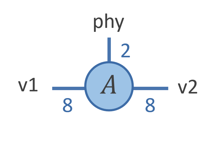
Consider a rank-3 tensor A as shown in Fig. 2 with indices labeled by “v1”,“phys”,“v2” and dimensions respectively. The following code example (Listing LABEL:code:rank3tensor) shows how to create a UniTensor to represent such a tensor and initialize all the tensor elements to one.
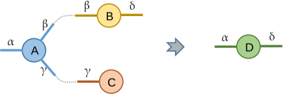
One of the most important operations in tensor network algorithms is the tensor contraction. It is an operation that sums the product of tensor elements over some common indices. For example, consider the contraction of three tensors , , and :
| (2) |
In this example, has three indices labeled by , , and . has two indices labeled by and , and has one index labeled by . Equation 2 defines a tensor contraction that sums over the common indices and , and the result is a tensor with two indices labeled by and . The corresponding graphical notation is shown in Fig. 3. Indices that connect two nodes are assumed to be summed over. The dashed lines indicate the connection of two bonds with the same indices to be summed.
Cytnx provides several methods for tensor contractions. One can use Contract or Contracts to perform simple contraction of two or more tensors respectively. They sum over common labels on these tensors. These functions are easy to use and make the code readable. The following code example (LABEL:code:contract) demonstrates the contraction of three tensors A, B and C. We note in passing that the user needs to take care of the correct index labeling in advance. See Sections 7.1 and 7.2 for details.
In a realistic algorithm, the number of tensors in a tensor network contraction can be quite many. The overall contraction is typically implemented in a sequence of binary contraction of tensors. However, the order of these binary contractions is not unique, and the computational costs depend strongly on the contraction order. One typically needs to first find an optimal contraction order before implementing the contractions.
In Cytnx, we introduce a powerful Network contraction method, which allows one to define a tensor contraction in an abstract way. The actual tensors to be contracted do not need to have a certain index order or specific labels. Consequently, the same Network object can be reused for successive contractions. Moreover, the contraction order can be optimized automatically. When a Network contraction is launched, it computes an optimized contraction order by a Dynamic Programming Algorithm. The optimized order can be saved and re-used for the subsequent contraction of the same Network with different tensors.
Using Network to perform a tensor contraction includes three steps: 1) Define a network, 2) load the tensors by PutUniTensor, and 3) launch the contraction. In what follows we briefly introduce how to use Network. Further details and a more complicated example of a contraction from an actual tensor network algorithm are discussed in Sec. 8.
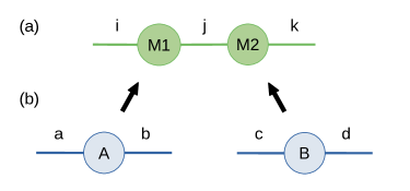
In this example, the goal is to use Network contraction to multiply the tensors and and sum over the common index , as shown in Fig. 4. One first creates a file matmul.net with content as shown in LABEL:code:netfile. Note that a Network is just a blueprint of the tensor contractions. In the code example (LABEL:code:MM) below, we first create a Network object using the file matmul.net. Then, we initialize two rank-2 UniTensor A and B. We specify the UniTensor objects that are actually to be contracted, by loading them into the Network and match the indices by their labels. In this step, the indices have to be assigned in the right order. In particular, we specify A (B) as M1 (M2) in the network. The indices a and b (c and d) are associated to the indices i and j (j and k). After loading the tensors, we launch the contraction and receive the result as a tensor AB whose indices are labeled by i and k.
Note that the indices a, b, c, d of the actual UniTensor objects are independent of the indices i, j, k defined in the network. With this design, one can implement an algorithm with meaningful index names, independent of the actual tensors to be contracted later on. On the other hand, a Network can be reused and loaded with different tensors and label conventions. As shown in code example LABEL:code:M2M1, the same Network object can be used to perform the multiplication BA instead of AB without relabeling.
3 Conventions and object behavior
In this section we discuss the naming conventions of Cytnx and the object behavior.
3.1 Naming convention
Generally, the function names in Cytnx follow these rules:
-
•
If a function is acting on objects, its name starts with a capital letter. For example, Contract(A,B) contracts two tensors A and B.
-
•
If a function is a member function or a generating function, it starts with a lowercase letter. For example, UniTensor.permute([1,0]) permutes the indices of a UniTensor object, where permute is a member function. uT=cytnx.UniTensor.zeros([2,2]) generates a UniTensor uT, so zeros is a generating function for the UniTensor object.
-
•
Types defined in Cytnx always start with capital letters. For example bd=cytnx.Bond(10) creates an object of Bond type.
-
•
If a function name does not end with an underscore, it will not change the input object. For example, B=A.permute([1,0]) creates a new object B that is A after permutation, while A remains unpermuted.
-
•
A function that ends with an underscore indicates one of the following scenarios:
-
1.
The input object will be changed. For example, cytnx.linalg.Pow_(A,2) replaces A by . Compare with Asq = cytnx.linalg.Pow(A,2), which creates a new tensor and leaves A unchanged.
-
2.
For a member function, it is an in-place operation. For example, A.permute_([1,0]) changes A by permuting its indices. Member functions which end with an underscore return a reference to themselves.
-
1.
3.2 Object behavior
In order to have a similar syntax and API in C++ and Python and to reduce the redundant memory allocation, all objects in Cytnx are references. The only exceptions are Accessor and LinOp. In Python, all objects are references by default already. On the C++ side, however, the reference character has to be implemented by Cytnx explicitly. For example, consider a UniTensor object in Python and C++ respectively.
It is apparent that a line to line translation between C++ and Python can be done with minimal effort. To achieve this, we implement the assignment "=" on the C++ side such that is a reference to . This also avoids copying of data. Additionally, Cytnx implements the is clause in the C++ API. This way, one can use is to check if two objects reference to the same memory. These additional implementations ensure that C++ and Python can have the same behavior.
In case where a copy of an object is needed, one can use clone as shown below. The functions is and clone support all objects of Cytnx.
Member functions which only change the metadata of a tensor (e.g. permute, reshape, relabel) create a new tensor with independent metadata. However, the new and old tensors share the same memory for the tensor elements. Thus, changing the elements of the new tensor will change the elements of the old one as well and vice versa. Changes to the metadata do not affect the other tensor though. If the tensor elements of the old and new tensors shall be independent of each other, use clone. Member functions which end with an underscore (e.g. permute_, reshape_, relabel_) change the tensor directly and return a reference to it, so no independent metadata is created. For example, we permute a tensor and change an element to see the behavior of the functions:
4 Non-symmetric Bonds
In Cytnx, a Bond represents an index (or axis, as in the NumPy convention) of a tensor. A Bond carries information about the dimension of a given index, which is the number of possible values the index can take. Moreover, bonds can have a direction, distinguishing incoming and outgoing indices of a tensor. When symmetries shall be preserved, the Bond objects carry additional information like quantum numbers associated with the symmetries. Bonds with symmetries are explained in Sec. 6.2. Here, we focus on bonds without symmetry properties. Bond objects can be used to initialize a UniTensor, see Sec. 5.
For a bond without quantum numbers, one can define a Bond object simply by specifying its dimension. Additionally, bonds can be directed and either be incoming or outgoing. If only the bond dimension is specified, the type is always REGULAR and thus un-directed. A directed bond can be created with cytnx.BD_IN or cytnx.BD_OUT. In this case, an outgoing bond can only be contracted with an incoming bond with the same size. When using symmetries, the bonds must be directed.
Combining bonds.
One can combine two bonds to create a new bond. The dimension of the new bond is the product of the dimensions of the input bonds, as illustrated below (LABEL:code:cd):
Moreover, an existing bond can be modified by merging another bond:
It is also possible to combine several bonds to create a new bond, or to modify an existing bond by merging several bonds. In this case, a list of Bond objects is used as the argument, as illustrated below (LABEL:code:bonds):
5 Non-Symmteric UniTensor
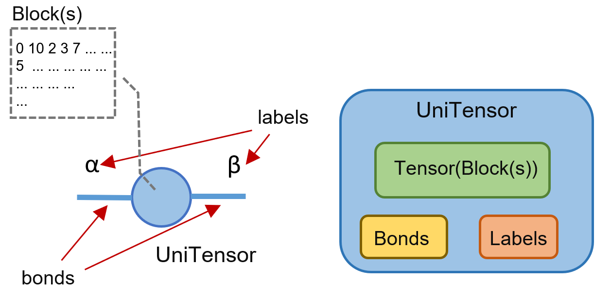
UniTensor is the central object in Cytnx. It is designed to represent all necessary information of a tensor so that tensor manipulations and calculations can be easily done. As indicated in Fig. 5, a UniTensor consists of three parts: Block(s), Bond(s), and Label(s). Additionally, each tensor can be given a name. Blocks contain the value of the tensor elements. Internally they are represented by Tensor objects (see Appendix A), which are very similar to NumPy.array or PyTorch.tensor. However, in typical situations the user does not need to interact directly with Tensor objects. Bonds are represented by Bond objects that define dimensions of the indices and can be directed as incoming or outgoing (see Sec. 4).
5.1 Creating a non-symmetric UniTensor
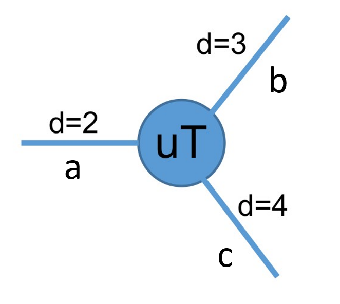
One can create a UniTensor through generators such as zero, arange or ones or eye. The first argument provides shape information, which is used to construct the Bond objects and to determine the rank – the number of tensor indices. Labels can be specified when creating a UniTensor, otherwise they are set to be "0", "1", "2", …by default. Consider a rank-3 tensor as shown in Fig. 6, the corresponding UniTensor can be created by the code example below (LABEL:code:UniTensorCreation).
Alternatively, we can also create a UniTensor by using Bond objects as shown in LABEL:code:UniTensorByBond. When a UniTensor is created from Bond objects, it is initialized with zeros by default. A Bond within a UniTensor can be accessed by UniTensor.bond.
In this example we show two ways to initialize the attributes of the UniTensor. We can either use the methods relabels to define the labels and set_name to set the name of a tensor as for uT2 in LABEL:code:UniTensorByBond. Or we set these properties with the arguments labels and name in the initialization method as for uT3 in LABEL:code:UniTensorByBond. We recommend the former way where methods are used subsequently. This way, the code can be ported between Python and C++ easily. In some cases (for example in LABEL:code:UniTensorCreation), the tensor has to be reshaped as well before the labels can be set, which is straightforward if the properties of the tensor are set by methods instead of initializer arguments.
Complex elements and data types.
We can create a UniTensor with a different data type, for example, with complex elements. This is achieved by setting the dtype argument when creating a UniTensor:
Random elements.
A UniTensor with random elements can be created easily. The code example below (LABEL:code:UniTensorRandom) demonstrates how to initialize a UniTensor with elements uniformly in the range [0, 1] or with elements from a Gaussian distribution with mean value 0 and standard deviation 1 respectively.
Moreover, one can randomize an existing UniTensor. This is particularly useful if a UniTensor is created from Bond objects, as it is typically the case for symmetric tensors. To obtain a UniTensor with random elements, one first creates a UniTensor, and then applies random.uniform_ or random.normal_ to it:
We note that random.uniform_ and random.normal_ work with UniTensor with and without symmetry. Real and complex date types of the UniTensor are supported. For complex data types, the real and imaginary part are randomized independently of each other.
5.2 Viewing/Changing labels
Indices can be addressed by their labels. To view the current labels and their internal order, one can use UniTensor.labels. Moreover, it might be necessary to change the labels for some bond(s). To change the label associated with one single bond, one can use UniTensor.relabel_, while UniTensor.relabels_ changes multiple labels associated with a list of bonds. In this code example, we show how to relabel one bond or multiple bonds and verify that the labels are changed correctly:
We may want to create a UniTensor from an existing one without modifying the original tensor, but we want to use a different set of labels. A typical situation where this is useful is the contraction of tensors by summing over common indices (see Sec. 7). Creating a copy of the tensor data is not desired, since it would double the memory usage. In such cases one can use relabel(s) without underscore. This returns a new UniTensor object with different metadata (in this case only the labels are changed), but the actual memory block(s) are still referring to the old ones. The arguments of relabel(s) are similar to relabel(s)_.
Users need to pay attention when using relabel for creating a UniTensor. Since the old and new tensors share the same memory for the data, any change of the elements in the new UniTensor affect the original UniTensor as well and vice versa. One can check if two UniTensors share the same data with
which will print True (False) if they share (do not share) the same memory for the data.
5.3 Permute
When a UniTensor is created, two important attributes are defined for each index: its position and label. We consider the code example LABEL:code:UniTensorCreation. The three indices bond1, bond2 and bond3 have positions 0, 1, and 2, and labels "a", "b" and "c" respectively. The library is designed such that users do not need to worry about the index positions in most applications. Instead, indices can be addressed by their labels. For example, tensor contractions can be defined purely by the index labels. However, the actual data in a UniTensor is stored as a multi-dimensional array (a Tensor object, see Appendix A) which has a specific order for the index positions. Conceptually, if one changes the index order of a UniTensor, it still represents the same tensor, but the way that the data is stored in memory is changed.
To specify the internal order of indices in a UniTensor, one can use UniTensor.permute. The new order can be defined by the index labels (strings) or the index positions (integers), as shown in the code example below (LABEL:code:UniTensorPermute). There, we use labels to see the new index order after calling UniTensor.permute. Note that the same labels can still be used to find the correct index even after a permutation. Therefore, all methods that use index labels do not need to be changed after a permutation.
5.4 Tensor information
Cytnx provides different ways to print information about a UniTensor. For the meta information but not the value of the elements, print_diagram can be used to visualize a UniTensor as a diagram. Consider the following code example and corresponding output (LABEL:code:print_diagram):
The command UniTensor.print_diagram shows information about the name, rank, block structure, diagonal form, and device.222name: can be set with set_name; rank: number of indices; block structure: used for a symmetric UniTensor, see Sec. 6; diagonal form: used to efficiently store diagonal matrices like the identity, singular values or eigenvalues; device: the data can be stored on the CPU or GPU memory, see Sec. 10 for details. Moreover, it prints a diagram of the tensor. The diagram provides visual information about labels, shapes, and rowrank.
The diagram shows that the indices are labeled by ["a", "b", "c"] with this internal order. They are ordered from upper left to lower left, and then from upper right to lower right. Typically, users do not need to know the internal order of the indices since bonds can be accessed by their labels instead. However, the index order can be used explicitly if needed. The integers inside the tensor show the dimension of the bond, such that one can read the shape [2, 3, 4] of the tensor from the diagram.
We observe that bond "a" is attached to the left of the tensor, while bonds "b" and"c" are attached to the right. This is controlled by a property called rowrank, which determines how to interpret a tensor as a matrix: The combination of the first rowrank bonds are interpreted as the row index, while the combination of the remaining bonds is interpreted as the column index. In the example above, the rowrank of the tensor is 1. This means that if we want to interpret this rank-3 tensor as a matrix, we get , where the matrix has row index and column index .
When a UniTensor is created, it acquires certain default rowrank. This plays a role only if a UniTensor is used in a linear algebra function, since it needs to interpret a tensor as a matrix. Consequently, before calling a tensor decomposition function, one may need to permute the labels and set the proper rowrank to ensure the correction mapping to a matrix. More details will be discussed in Sec. 9.
Moreover, one can use print to see the tensor elements as an -dimensional array:
5.5 Arithmetic operations and tensor operations
Cytnx supports basic addition (+), subtraction (-), multiplication (*), and division (/) operations for UniTensors. Note that all of these operators are element-wise, which means that the operation is applied between each pair of elements from the two UniTensors. Obviously, the two operated UniTensors must have the same shape. Other useful operations are UniTensor.Norm, which returns the two-norm of the tensor and UniTensor.Conj, which takes the complex conjugate of all elements (see Sec. 6.4 for an example). An extensive list of tensor operations and linear algebra functions is provided in the User Guide [39]. Further linear algebra functions are discussed in Sec. 9.
5.6 Getting/Setting elements
UniTensor.at().
To get or set a single element in a UniTensor, one can call UniTensor.at. It returns a proxy which contains a reference to the element, and therefore can be used to get or set the element. The first argument of UniTensor.at contains the labels of the bonds in the UniTensor, and the second argument contains the corresponding index values for the element one wants to access. For example:
Slicing.
To get or set a range of elements in a UniTensor one can use slicing, where the internal order of indices is used.
5.7 Accessing data in a block
The elements of a UniTensor are stored in a Tensor object. One can access and manipulate the Tensor as described in Appendix A and read and change the data of the UniTensor this way.
Getting a block.
The Tensor can be accessed by UniTensor.get_block and UniTensor.get_block_, where the first method returns a copy of the Tensor object in the UniTensor, while the second method returns a reference. As an example, we manipulate the Tensor in order to change an element of the UniTensor:
A UniTensor without symmetries contains only one block, while several blocks exist when symmetries are involved, see Sec. 6.3.3.
Putting a block.
The methods UniTensor.put_block() and UniTensor.put_block_() replace the data of a UniTensor by a Tensor. For example, after getting a block from a UniTensor, we can manipulate the corresponding Tensor object and write it back to the UniTensor:
We get the same output as in LABEL:code:get_block_, where we manipulated the reference to the block directly. Note that the shape of the Tensor has to match that of the UniTensor whose data shall be replaced.
5.8 Converting to/from a NumPy array
It is very easy to create a UniTensor from a NumPy array and vice versa. This is particularly useful for including existing code or when one wants to quickly test an algorithm using Python and then convert to Cytnx for acceleration, quantum numbers, or larger-scale applications. Such flexibility also allows users to make use of the tools from other packages like NumPy, SciPy and PyTorch. Since all popular tensor libraries allow for conversion of their containers to a NumPy array, the latter serves as a bridge to Cytnx. In the future, we plan to support PyTorch directly as the underlying container of a tensor in Cytnx. This way, users will be able to use automatic differentiation directly in Cytnx.
In LABEL:code:to_from_numpy we show an example where we create a NumPy array and then convert it to a UniTensor. The tensor corresponds to the matrix product operator that defines the Hamiltonian of the transverse-field Ising model [40].
6 UniTensor with Symmetries
In physics, systems are often symmetric under certain transformations. Exploiting such symmetries can be advantageous in many cases. Cytnx allows for the incorporation of the symmetries on the level of the tensors directly. We explain the basic concepts that are used in Cytnx. Further details on symmetries in tensor network algorithms are found in [41, 42].
According to Noether’s theorem, symmetries imply conserved quantities, for example, the total charge in the system. In that case, the Hamiltonian will have a block-diagonal structure where each symmetry sector has a definite charge (quantum number), which is caused by the fact that different charge sectors do not mix with each other. When the symmetric structure is imposed on the level of the tensors which describe the system, they become block-diagonal as well. This substantially reduces the memory costs and the number of variational parameters in numerical algorithms. Thus, larger system sizes or larger bond dimensions are accessible with the same computational costs. Moreover, numerical errors contributed by the elements that do not conserve symmetry (and hence are zero) can be avoided. Finally, simulations can be restricted to certain symmetry sectors if needed.
A quantum-number conserving tensor can be understood in the following way. By definition, each element in a tensor can be labeled by its index value for each index. For example T[0,0,0] is an element with index values 0 for all three indices. Consider that in addition to the integer, each index value also carries a quantum number. This is shown in Fig. 7, where bonds are indicated by directed arrows, and each index value, represented by a horizontal line, has an associated quantum number.
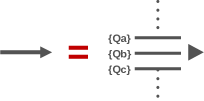
One can then define a quantum-number flux for each element by adding all the incoming quantum numbers and subtracting all the outgoing quantum numbers. Note that the rule of "addition" and "subtraction" actually depends on the symmetry group associated with the quantum number. For charge conservation, which is associated to a symmetry, addition and subtraction follow the same rule as for integers. The conservation of a quantum number is ensured by restricting the tensors to only have non-zero elements with zero flux. For these elements, the total quantum number flowing into the tensor has to be equal to the total quantum number flowing out. All other elements that do not conserve the charge must be zero. For a UniTensor, these zero-elements are not stored in memory. Therefore, a symmetric tensor can be thought of as a direct sum of blocks of different quantum-number sectors, as represented in Fig. 8.
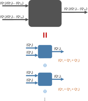
In Cytnx, symmetric UniTensors contain Bond objects which carry quantum numbers. The bonds themselves contain a Symmetry object describing all the symmetries involved. Currently, abelian symmetries are implemented in Cytnx. Non-abelian symmetries like are planed to be supported in the future [43]. Cytnx has predefined symmetry objects for and symmetries. Once a symmetric UniTensor is defined, it can be used just like before, with typically no changes in the API of functions. In particular, the linear algebra operations respect the block structure automatically.
Sometimes a quantum number flux which differs from zero can be desired. For example, an external field can change the flux locally. In these cases, an additional bond can be attached to the UniTensor, which has a dimension of one and carries the quantum number of the flux change. The code in LABEL:code:create_Hamiltonian_symmetric shows an example where this is used for particle number changing operators.
6.1 Symmetry and quantum numbers
The symmetry properties are contained in the Symmetry class and Symmetry objects are used in the construction of a Bond with quantum numbers. When a Symmetry object is printed, the name and type of the symmetry are displayed, as well as the combine rule and the reverse rule. The combine rule defines how two quantum numbers are merged to a new quantum number. For the additive quantum numbers of , the combine rule is simply the sum of the individual quantum numbers. The reverse rule defines how a quantum number is transformed when the bond is redirected. Quantum numbers on outgoing bonds have the reverse rule applied when they are combined with other quantum numbers. With this procedure, the symmetry preserving entries of a tensor are those where the combination of all quantum numbers is zero. For example, the inverse rule of takes the negative value of the original quantum number.
For example, we can create a Symmetry describing the group or :
6.2 Bond with quantum numbers
In Cytnx, the quantum number information is stored in the Bond objects. A Bond with quantum numbers must have the following properties defined:
-
1.
A direction. The bond is either incoming (BD_IN) or outgoing (BD_OUT).
-
2.
A list of quantum numbers and their dimensions. Quantum numbers are integers.
-
3.
The corresponding symmetry group(s), see Sec. 6.1.
A direction is essential for any Bond in a symmetric UniTensor. Symmetry preserving tensors have a block structure, which is determined by the requirement that for non-zero elements the total quantum numbers of the incoming bonds equals the total quantum number of the outgoing bonds. Thus, all entries that do not fulfill this condition have to vanish and the corresponding blocks do not need to be stored explicitly. By defining bonds with quantum numbers, a UniTensor created with these bonds will automatically have the desired block structure.
6.2.1 Creating bonds with quantum numbers
We consider as an example a tensor with symmetry. We would like to construct a bond for which the subspace with quantum number has a dimension (or degeneracy) of 3, while the subspace has dimension 5. We can create the bond using a list to describe the quantum numbers [[2],[4]] and another list containing the dimensions [3,5]. Note that the quantum number is enclosed in a list to accommodate multiple symmetries. Instead of the two lists, we can also use a single list of tuples where each tuple combines the information of quantum number and dimension [([2],3),([4],5)]. Cytnx also includes a helper function Qs to allow for a simpler and well readable syntax. The code [cytnx.Qs(2)>>3, cytnx.Qs(4)>>5] generates the aforementioned list of tuples.
The symmetries and the corresponding quantum numbers are encoded by lists. This way, multiple symmetries can be present at the same time. Consider a tensor with symmetry. We specify the symmetry by [Symmetry.U1(), Symmetry.Zn(2)]) and the quantum numbers by [q_U1, q_Z2]. We can use Qs(q_U1, q_Z2)>>dim to construct the tuple containing the quantum numbers and the dimension of the subspace. One can print a bond to check its quantum numbers.
6.2.2 Combining bonds with quantum numbers
Bonds with symmetries can be combined. The new quantum numbers are the combination of the two input quantum numbers. The actual combine rule depends on the corresponding symmetry group. For for example, two quantum numbers are combined by adding them. In general, different pairs of quantum numbers can be combined to the same quantum number. For example, both and give the quantum number in the case. Therefore, the output bond in general can have several quantum-number sectors with the same quantum number. By default, the sectors with the same quantum numbers will be grouped into a single sector with accordingly increased dimension. However, users can choose not to group them by setting the argument is_grp=False. Here is an example of how to combine two bonds with is_grp=True (default) and is_grp=False:
In the example we print the Bond objects to check their quantum numbers and the corresponding dimensions. We can see that the output quantum numbers are the sums of the input ones, and the sectors with the same quantum numbers are grouped or not depending on the argument is_grp=False. Note that the number of sectors (3 for bond12 and 4 for bond12_no_group) can differ if is_grp is changed.
Note that only Bonds with the same direction can be combined, and the resulting Bond will have the same direction. In a physical interpretation, an incoming or outgoing Bond can be used to define the Hilbert space for a ket or a bra state, respectively. In this sense, combining two Bonds represents a product of Hilbert spaces for the two states, which is well defined only if both states are ket or bra states.
6.2.3 Redirecting bonds
One can change the bond direction by using Bond.redirect or Bond.redirect_:
6.3 Symmetric UniTensor
6.3.1 Creating a symmetric UniTensor
A symmetric UniTensor is created with Bond objects which carry quantum numbers. Conceptually, one needs to identify the symmetries (for example, symmetry) in the system, and then specify the dimensions of all quantum number sectors for the bonds. As an example, we consider a rank-3 tensor with symmetry. The first two bonds are incoming bonds with two quantum number sectors and , both with dimension . The third bond is an outgoing bond with three quantum number sectors , , and , with dimensions , , and respectively. We then initialize a UniTensor using these three bonds.
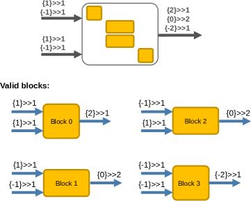
For this UniTensor, there are 4 valid blocks that carry zero-flux and thus can have non-zero elements that do not break the symmetry. Figure 9 shows the block structure and the corresponding quantum numbers for each block. We can use UniTensor.print_blocks to see all the blocks and their corresponding quantum numbers:
The block index is printed as BLOCK [#], and the number in the square bracket [] beside each bond is called a Qn index (quantum number index). Qn indices are used to access the sectors in a bond. Consider the third bond (the out-going bond) as an example. It has three possible values for the quantum number: , , and . It is created with this particular ordering of the quantum numbers. Hence, Qn=0 corresponds to the quantum number , Qn=1 to the quantum number , and Qn=2 to the quantum number . Both the block index and the Qn indices can be used to access a block in a UniTensor as it will be described below in Sec. 6.3.3.
6.3.2 Accessing elements of a symmetric tensor
The UniTensor.at method works in the same way as without symmetries (see Sec. 5.6). For a symmetric UniTensor, some elements may not exist due to the quantum number constraint. If one tries to access an element that does not correspond to a valid block, an error is thrown:
However, one can use the proxy to check whether an element corresponds to a valid block with symmetries:
This way, one can make sure that an element is part of a valid block before the data is accessed.
6.3.3 Accessing blocks of a symmetric tensor
Getting a block.
A symmetric UniTensor contains multiple blocks for different quantum number sectors in general. We can use the methods get_block and get_block_ to access the blocks. Compared to the non-symmetric case in Sec. 5.7, her we have to specify the block for a symmetric UniTensor. Note that get_block returns a copy of the Tensor object, while get_block_ returns a reference. We use the symmetric UniTensor from the example in LABEL:code:symmTensor to demonstrate how to access blocks. There are two ways to get a certain block from a symmetric UniTensor: by its Qn indices or by its block index. When using Qn indices, the labels of the indices can be given as the first argument of get_block, followed by a list of the Qn indices associated with the block.
One can also access all valid blocks in a symmetric UniTensor with get_blocks or get_blocks_. These methods return a list (or a vector in C++) of blocks, where each block is a Tensor object. The blocks are ordered with ascending block index, corresponding to the order in which they are stored in the UniTensor. This order can be checked by UniTensor.print_blocks().
Putting a block.
Similarly to the non-symmetric case, we can put a Tensor as a block to a UniTensor. In the symmetric case, one can put a Tensor to a particular block by specifying the Qn indices or the block index:
6.4 Change the bond direction
One can change the direction of all bonds with UniTensor.Transpose or UniTensor.Dagger. The latter returns the Hermitian conjugate of a UniTensor, with all bond directions inverted and the complex conjugate of all elements taken. For tensors with non-directional bonds (REGULAR type), the bonds remain non-directional after the operation. If only the complex conjugate of a tensor is desired, UniTensor.Conj can be used. If the dtype of the tensor corresponds to real valued elements, the complex conjugation has no effect. In line with the general naming convention, UniTensor.Transpose_, UniTensor.Conj_ and UniTensor.Dagger_ change the tensor in-place. The following code shows an example for the UniTensor.Transpose, UniTensor.Conj and UniTensor.Dagger operations:
6.5 Conversion between UniTensor with and without symmetries
One can use UniTensor.convert_from to perform conversion between UniTensors with and without symmetries. If one tries to convert a non-symmetric UniTensor with non-zero elements in the symmetry violating blocks to a symmetric one, an error is thrown. It is possible to overwrite the check by using keyword argument force=True. In this case, the elements in the symmetry violating blocks are ignored.
As an example, we first create a non-symmetric UniTensor, which represents the two-site Hamiltonian . We initialize the -matrices, take Kronecker products of pairs of them, and then sum the terms to get the Hamiltonian:
This non-symmetric UniTensor can be converted to a symmetric one, which has to be initialized with the correct quantum numbers. In our case, we create a symmetric UniTensor and copy data from the non-symmetric UniTensor:
Similarly, we can directly create a symmetric UniTensor, which represents the previous Hamiltonian. This time, the -matrices need to be symmetric tensors which carry quantum numbers. The and operators change the quantum number locally. In this case, we can see them as creation and annihilation operators, which change the particle number. Thus, the corresponding tensors would naively not conserve the quantum number. However, we can attach an additional bond with only one index to these -matrices, whose quantum number corresponds to the local particle number change (bqo or bqi in LABEL:code:create_Hamiltonian_symmetric). We observe that the terms of the Hamiltonian only contain pairs which involve one and one operator. The Hamiltonian thus conserves the particle number, which makes it a good quantum number. We can use this to make sense of the previously introduced quantum number changing bonds: each tensor needs to have such an additional bond, which is contracted with the additional bond of a tensor according to the terms of the Hamiltonian. The following code example demonstrates this:
Finally, we can convert the symmetric UniTensor into a non-symmetric one and compare to our previous initialization of the Hamiltonian:
The conversion between symmetric and non-symmetric can be very useful, for example for conveniently checking the elements of a symmetric UniTensor in matrix form. We note, however, that performing operations on non-symmetric tensors and then converting them to symmetric ones can lead to problems. This can, for example, happen, when linear algebra routines are performed on non-symmetric tensors. Numerical errors or simply the fact that symmetry violating elements are not explicitly forbidden can lead to non-zero elements in the wrong blocks. Even when these are ignored using the argument force=True, errors can accumulate in tensor network algorithms. We therefore suggest to avoid convert_from when possible and only use it with care. Symmetric tensors should be used wherever symmetries shall be preserved. Cytnx provides linear algebra routines that preserve the symmetries of the tensors. If operations are needed that are not natively supported by Cytnx, these should be operating on the level of the blocks to make sure symmetry violating elements can not arise.
Besides avoiding numerical errors, symmetric tensors also help in the code development by ensuring that only operations are allowed which respect the symmetries. For example, the and operators in LABEL:code:create_Hamiltonian_symmetric can only come in pairs, such that their additional indices are contracted. Otherwise, open indices arise that still need to be contracted with suitable operators. This behavior is much less error prone than using non-symmetric tensors which allow for any operation, including symmetry violating ones.
7 Tensor contraction
All tensor network algorithms include tensor contractions, where we multiply tensors and sum over shared indices. Cytnx provides three different ways to perform these contractions. A simple way to contract indices is provided by Contract and Contracts. These functions contract two or more UniTensor objects by summing over all indices that have the same label on two of the tensors. We also support the API of ncon which allows users to contract tensors by defining the connectivity and contraction order of the bonds. We refer to the User Guide [39] for the detail. Since the user needs to specify the bonds by their indices instead of their labels, so the index order matters. This can be error prone when users have to keep track of the change of the index order in complicated tensor network algorithms. In Cytnx we introduce an advanced method for tensor network contractions via a Network object. It is particularly useful for contractions involving many tensors and reusable contraction diagrams. The Network based contraction will be explained in more details in Sec. 8.
7.1 Contract
Two tensors can be contracted with Contract as shown in the code example in LABEL:code:contractTwoTensors. Using this function, common indices of the two tensors are summed over. A new UniTensor is created to represent the result, while the input tensors are not modified. The labels of the output tensor are inherited from the input tensors. In order to avoid potential mistakes, Cytnx checks that the dimensions of the contracted indices are the same before running a contraction. For symmetric tensors, Cytnx also checks the bond direction, the quantum numbers, and the dimensions of each symmetry block.
In some scenario, one may need to change the labels of the input tensors for the contraction, while the labels of the original tensors shall stay unchanged. In this case, one can use UniTensor.relabel to obtain a UniTensor with new labels but without actually copying the data (see Sec. 5.2). Alternatively, a Network can be used where no initial relabeling is needed, see Sec. 8.
7.2 Contracts
Contracts provides the same functionality as Contract but allows users to contract multiple tensors. The first argument of this function is TNs, which is a list containing all UniTensors to be contracted. There are two further, optional arguments: order (string), which specifies a desired contraction order, and optimal (True or False; default True), for specifying if one wants to use an automatically optimized contraction order. Since, the contraction order is given in terms of the names of the UniTensors, the names have to be set for all tensors involved the contraction; otherwise a run-time error is raised. If optimal=True, a contraction order is computed in every function call, which creates some unnecessary overhead if a similar contraction is executed several times. In these cases, we recommend using a Network object for the contraction (see Sec. 8), where the optimal order can be calculated in the first run and be reused for consecutive contractions. When a specific order is given, the optimal argument should be set to False.
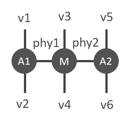
As an example, consider a contraction consisting of tensors A1, A2 and M as sketched in Fig. 10. The corresponding code example is shown in LABEL:code:UniTensorContracts.
8 Network
Cytnx makes it easy to design, implement, and optimize the contraction of sophisticated tensor networks via the Network object, which contains the blueprint of the corresponding tensor network. A Network can be created from a string or a plain text file, which contains the description of the network in a human readable format. The Network can be displayed as well to check the implementation. One can contract multiple tensors at once with a Network. Furthermore, the contraction order can either be specified by the user, or an optimal order can be generated automatically. A Network is particularly useful when the same kind of tensor network contraction has to be performed repeatedly, but with different tensor objects each time. We can define the Network once and reuse it for several contractions. The contraction order can be optimized once after the first initialization with tensors. In the proceeding steps, this optimized order can be reused.
Using Network to perform a tensor contraction includes three steps. First, we need to define the target tensor network and create a Network object. Second, we need to load (put) the actual UniTensors that are to be contracted. Finally, we launch the contraction. In the following we explain these steps in more detail.
8.1 Creating a Network
The creation of a Network object is demonstrated with an example here: we use a Network to perform two matrix-matrix multiplications for three rank-2 tensors , , and at once. The outcome is also a rank-2 tensor. The network diagram and its output tensor are shown in Fig. 11. The code example in LABEL:code:NetworkMMM shows how to create a corresponding Network object from a string. One can print the network to check the structure.

The contraction is defined by the rule that all the common indices are summed over, and the remaining indices will be the indices of the output tensor. The keyword TOUT is used to specify the order of the remaining indices that are not summed over. In this example, indices labeled by i and j are not contracted and they become the first and second index of the output tensor. Consequently, if the output tensor represents a scalar (rank-0 tensor), no labels should be given after TOUT:. The keyword ORDER is used to specify a user-defined contraction order. If nothing is specified after ORDER:, the default order is contracting the tensors in the order of their appearance in the creation of the Network. One can modify the ORDER after the creation of the Network or let Cytnx find an optimal contraction order after all tensors are loaded, see Sec. 8.3.
One can also create a Network object from a file. For this, the same content as in the aforementioned network creation string (LABEL:code:network_file) is written to a plain text file. Here, we name the file example.net. Such a network file can then be loaded with the Network initializer or by using Network.Fromfile. One can also write a Network object to a network file using Network.Savefile. The code example below (LABEL:code:NetworkFile) illustrates loading and saving a network file.
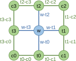
To further demonstrate the power of Network, we consider a contraction that appears in the corner transfer matrix algorithm [44, 45]. The tensor network diagram is sketched in Fig. 12. In the code example below (LABEL:code:CTM), we create a Network from a string for this case. The example demonstrates that it is also straightforward to translate a more complicated network diagram into a string, which defines the corresponding Network. The Network object is thus particularly useful for algorithms in higher dimensions, where many tensors need to be contracted. We note that in the case shown here, TOUT: is empty because the outcome tensor is a scalar.
We emphasize that the labels used in the Network are dummy indices only for the network, and are completely independent of the labels in the UniTensor objects that are going to be contracted. This design gives us the flexibility to define a Network object without knowing the labeling conventions of the UniTensors to be contracted. In particular, the Network can be loaded with different UniTensors for each contraction and be reused.
8.2 Putting UniTensors and performing a contraction
A Network is a skeleton that does not contain the actual tensor objects to be contracted. To perform the contraction, one needs to specify a UniTensor object for each tensor defined in the Network, and make a connection between the dummy indices in the Network and the actual indices of the UniTensors. This is done by using Network.PutUniTensor. To give an example, we consider the Network defined in LABEL:code:NetworkMMM and the following UniTensors which shall be contracted:

Note that the indices of A, B, and C have common index labels and . This is often the case in certain tensor network applications. We load the Network with the specific UniTensors by using Network.PutUniTensor for each tensor individually. The first argument is the name of the tensor to be specified in the network, and the second argument is the UniTensor object as a realization of that tensor. The third argument is a list of the labels in the UniTensor in the order of the indices of the Network. For example, A is a realization of M1, and the indices a and b in A correspond to the indices i and j in M1. Similarly, B(C) is a realization of M2(M3), and the indices a and b in B(C) correspond to the indices j(k) and k(l) in M2(M3). When all tensors in the network are specified, one can perform the contraction by simply calling Network.Launch to obtain the result. Note that the output tensor inherits the index order and labels from the specifications following TOUT:.
8.3 Setting the contraction order
The efficiency of a tensor network contraction depends on the order of the contractions. This order can be specified when the Network is defined (see Sec. 8.1). However, one can also reset the contraction order using the method Network.setOrder. A certain contraction order can be forced in the same way as explained in Sec. 8.1. Alternatively, one can let Cytnx compute the optimal order by setting Network.setOrder(optimal=True). Note that in this case, the optimal order will be computed (and stored) every time when a contraction is launched. This is necessary because the optimal order depends on the bond dimensions of the input tensors, which can be different for each contraction. In practice, one often increases the dimensions of the indices during the simulations until they are kept constant when they reach a certain value. Then, the optimal contraction order typically does not change anymore. In this cases, one can set Network.setOrder(optimal=True) up to some large enough bond dimensions, and then set Network.setOrder(optimal=False) such that the Network will no longer compute the optimal order before the contractions, but just use the stored contraction order. Similarly, the dimensions do not change when a network contraction is used in an iterative solver many times. Then, the contraction order only needs to be optimized in the first iteration. One can check the current contraction order using Network.getOrder:
8.4 Advanced example: Expectation value of a Projected Entangled Pair State
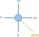
In this advanced example, we show how a more complicated tensor network contraction can be implemented by using Network. Specifically, we consider the contraction for the expectation value of a two-dimensional tensor network state. Physical states in two spatial dimensions, in particular ground states, can be approximated by a Projected Entangled Pair State (PEPS) [46]. This tensor network consists of one tensor at each lattice site. One index of each tensor corresponds to the physical degrees of freedom at this site (dotted lines in Figs. 14 and 15). Further internal bonds connect each tensor to its nearest neighbors. Fig. 14 shows a PEPS tensor in two spatial dimensions.
A typical PEPS algorithms prepares a desired state, for example the ground state of a Hamiltonian. Then, expectation values are measured as the quantities of interest for physics [1]. The boundary matrix product state (boundary MPS) method is used to efficiently calculate expectation values. See Ref. [47] as an example of a finite lattice PEPS calculation with more details on the algorithm.
The expectation value of a nearest neighbor operator corresponds to the tensor network in Fig. 15. Here, the blue tensors and are the PEPS tensors that the operator acts on, while the starred versions are there complex conjugate counterparts. The green tensors to represent a boundary matrix product state, which is used to approximate the PEPS tensors at the remaining sites.
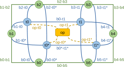
The diagram in Fig. 15 can directly be translated into a Network file. One writes the names of the tensors and their indices one by one to the file:
The actual contraction is done by loading the Network file and using PutUniTensor with the correct UniTensors. This way, the expectation value can be calculated for tensors at different sites, and also other naming conventions of the indices could be used without changing the format of the Network file. Our index labeling convention for the PEPS tensors can be seen in Fig. 14. The names of the boundary MPS tensors start with "bMPS" in our convention, and the index labels indicate to which kind of tensor the index connects to.
When loading the actual tensors, the indices of a UniTensor have to be assigned to the corresponding ones in the Network. This can simply be done by the index labels in the correct order as the third argument of net.PutUniTensor. Figure 16 shows an example for this mapping. The code to put the UniTensors and launch the contraction is shown below in LABEL:code:peps_contraction.

The diagram in Fig. 15 is intended for calculating an expectation value of an operator that acts on a nearest-neighbor pair in x-direction. However, the same Network file can be used also for operators acting in y-direction. Only the arguments of PutUniTensors need to be adapted. This way, tensor diagrams can be implemented as network files and be used flexibly, without the need to rewrite them for different tensors to be loaded. Also, the user does not need to care about the index order inside the UniTensor if labeled indices are used.
9 Tensor decomposition and linear algebra
Tensor decompositions by linear algebra algorithms are essential ingredients in tensor network applications. Cytnx supports an extensive list tensor operations and linear algebra functions and we refer to the User Guide [39] for the complete list and further documentation. Typically, linear algebra functions require matrices as input. Consequently, before calling a linear algebra function, Cytnx internally maps a UniTensor to a matrix. In Sec. 9.1 we explain how to ensure that the correct mapping is carried out. Then, we show how to perform singular value decomposition (SVD) (Sec. 9.2), eigenvalue decomposition (Sec. 9.3), and QR decomposition (Sec. 9.4) respectively.
9.1 Mapping from tensor to matrix
Cytnx provides several linear algebra functions and tensor decomposition methods. The library calls established and well optimized linear algebra functions, which require matrices as input. Therefore, the tensors need to be represented by matrices in any of the methods. This is done by classifying each index in a tensor to be either part of the resulting row index or column index, and then combining all the row (column) indices into one row (column) index for the matrix representation. The dimension of the final row (column) index is the product of the dimensions of all the original row (column) indices.
The UniTensor objects have an attribute called rowrank to control the mapping from a tensor to a matrix. In matrix representation, the first rowrank indices are treated as row indices, and the remaining indices are treated as column indices. There are different ways of mapping a tensor to a matrix depending on which indices are selected as row or column indices. Before calling a tensor decomposition method, one needs to prepare the tensor such that it has the desired mapping. This is done by 1) permuting the indices such that all the row indices are in front of all the column indices, and 2) setting rowrank to the number of row indices by using UniTensor.set_rowrank or UniTensor.set_rowrank_.
The following example shows how to prepare a specific matrix representation of a rank-3 UniTensor, where one of the indices is interpreted as the row index and the other two indices form the column index:
We see that M.rowrank return the rowrank information, which is also encoded in the diagram created by UniTensor.print_diagram – the indices at the left (right) side are the row (column) indices.
9.2 Singular value decomposition
Without truncation.
The singular value decomposition (SVD) decomposes a matrix into the product of three matrices , , and (i.e., ), where is a diagonal matrix and its non-negative elements are called singular values. and satisfy and with the identity matrix. In Cytnx, one can perform a SVD by using the function linalg.Svd. There is an optional argument is_UvT (default True): If is_UvT=True, the function returns three tensors , , and ; if is_UvT=False, the function returns only the singular-value tensor . Note that this function does not perform any truncation. We also note that inherits the row labels of , while inherits the column labels of . The other labels are automatically generated in such a way that one can use Contracts to perform the matrix multiplication of , , and . However, the indices after the contraction with Contracts might have a different order and need to be permuted before comparing to the original tensor . The following example shows how to perform a SVD of the previously created rank-3 tensor:
With truncation.
In practice, one often uses a SVD as an approximating method by truncating the linear space based on the singular values. A SVD with truncation can be executed by calling linalg.Svd_truncate. This function performs a full SVD of the initial tensors, and then truncates it to keep only the largest singular values. linalg.Svd_truncate has several additional arguments:
-
•
keepdim specifies the maximal dimension to be kept after the truncation.
-
•
err defines the threshold for singular values to be kept; the linear space with singular value smaller than err will be truncated. Note that the singular values are not normalized before the truncation.
-
•
return_err; for return_err=1, the function returns an additional one-element UniTensor that stores the largest of the truncated singular values; for return_err=2, a UniTensor containing all the truncated singular values is returned instead; for return_err=0 (default), no truncation error is returned
Here is an example of an SVD with truncation:
9.3 Eigenvalue decomposition
The eigenvalue decomposition, also known as matrix diagonalization, is defined for square matrices only. It decomposes a square matrix to , where is a diagonal matrix and its elements are called the eigenvalues. The columns of correspond to the right eivenvectors of . If is a Hermitian matrix, all the eigenvalues must be real, and becomes a unitary matrix satisfying . Consequently for a Hermitian matrix.
One can perform the eigenvalue decomposition by using linalg.Eig for a generic square matrix or linalg.Eigh for a Hermitian matrix. Since the input matrix must be a square matrix, the row and the column dimensions in the matrix representation must be equal; otherwise, an error is raised. One can use the optional argument is_V (default True) to determine if the eigenvector matrix shall be returned. A complete description of the optional arguments can be found in the User Guide [30]. Here is an example of an eigenvalue decomposition of a Hermitian matrix:
If one is only interested in the lowest few eigenvalues, it can be very inefficient to first execute the contraction of a tensor network to obtain a matrix and then pass this matrix to the eigenvalue decomposition function. Methods like the Lancsoz solver for finding the smallest eigenvalues only require a linear operator, which defines how a vector is transformed. This can be a matrix multiplication, but also a more complicated tensor network contraction or any general linear transformation of the input vector. Cytnx provides a way to define such an operator as a LinOp object and pass it to the Lanczos linear algebra function to find the lowest few eigenvalues and corresponding eigenvectors of a Hermitian linear operator. More details and example code can be found in the User Guide [49].
9.4 QR decomposition
The QR decomposition decomposes a matrix to the form , where is a column-orthogonal matrix (), and is an upper-right triangular matrix. One can perform a QR decomposition by using cytnx.linalg.Qr:
10 Device and GPU support
In Cytnx, the tensor elements can either be stored in the memory accessible to CPUs or GPUs. The use of GPUs can speed up tensor contractions and therefore shorten the run-time of tensor network algorithms. Using GPUs is very simple in Cytnx: After creating a tensor directly on a GPU or moving a tensor from CPU to GPU, the functions and methods provided by Cytnx can be used without any changes of the API. Therefore, tensor network algorithms can easily be ported to GPUs by only changing the initialization step of all tensors. For example:
Since tensor elements can be stored in the memory of a given CPU or GPU on multi-CPU/GPU systems, it is important that the user ensures tensors are on the same device when they are used together in contractions or linear algebra functions. In Cytnx, the object cytnx.Device handles all device properties. The Device of a UniTensor can be seen when printing the tensor by print_diagram or print (see Sec. 5.4).
10.1 Device status
Number of threads.
To see how many threads can be used in the current program by Cytnx, one can check Device.Ncpus.
Number of GPUs.
The number of GPUs available to Cytnx in the current program can be checked with Device.Ngpus.
If Cytnx is not compiled with CUDA available, Device.Ngpus returns 0.
10.2 Initializing tensors on CPU and GPU
For the GPU computations, Cytnx uses the Magma [50] library as well as several CUDA based third-party libraries like cuBlas [51], cuSolver [52], cuTensor [53] and cuQuantum [54]. The performance of tensor network algorithms implemented in Cytnx can be significantly accelerated when using GPUs, as shown in Sec. 11. Developers of tensor network algorithms can directly benefit from the GPU acceleration.
Users can easily transfer tensor network algorithms implemented in Cytnx from the CPU to GPU version with minimal code modifications. Cytnx provides two ways to create objects on GPU devices: either by initializing objects on a GPU directly or by using the to() method to convert objects stored in the CPU memory.
Initializing tensors on a GPU.
UniTensor objects with data stored in the GPU memory can be created with the argument device in the initialization step. For example:
Other initialization methods like ones, arange, ones, uniform, normal, or eye can be used similarly.
Data Transfer between Devices.
The library provides a convenient way to move the data of Cytnx objects between CPU and GPU with the to or to_ methods. For example, we create a UniTensor in the memory accessible by the CPU and transfer it to the GPU with gpu-id=0:
If only specific parts of an algorithm are suitable for GPU simulation, it is recommended to use the to method to transfer the objects between CPU and GPU.
11 Benchmarks
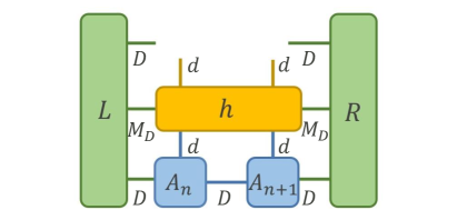
To test the performance of Cytnx, we compare the execution times of two typical tensor operations in Cytnx and ITensor[31] on a CPU and on a GPU. ITensor is implemented in both Julia and C++. In this comparison, we use the C++ version of ITensor (v3.0.0). One of the main applications of tensor networks is to use them as a variational ansatz for a quantum many-body state. Here we benchmark the performance on a variational method, the density matrix renormalization group (DMRG) [55, 2], which computes the ground state of a given Hamiltonian within a tensor network approximation. In particular, we consider the one-dimensional XX model with spins:
The Hamiltonian conserves the total spin in the direction, which can be used as a quantum number. In a DMRG algorithm, one represents the ground state as a network of tensors , where . These tensors are updated sequentially from one boundary to the other in a DMRG sweep. An essential step in the DMRG sweep is the update of two tensors and , where a tensor contraction as sketched in Fig. 17 is needed. In the figure, , , and correspond to the physical dimension, bond dimension and MPO bond dimension respectively. Since the bond dimension is related to the accuracy of the DMRG algorithm, we use as the control parameter in the benchmark. It is expected that the computational time scales as for large . An implementation of DMRG using Cytnx can be found in the examples section in Cytnx’s User Guide [30].
CPU Benchmark.
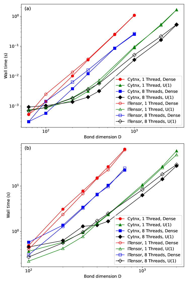
We first benchmark the performance on an Intel(R) Core i7-9700 CPU. We perform the test with symmetric tensors which preserve the total spin, as well as unconstrained tensors without explicitly implemented symmetries. In Fig. 18 (a), we show comparisons of wall times for the tensor contraction sketched in Fig. 17, as a function of on a log-log scale with Cytnx and ITensor. One can see that the performance of the two libraries is very similar. As expected, using symmetric tensors can reduce the computational costs except for very small bond dimensions. The parallelization with 8 threads reduces the execution time for the contraction compared to the single threaded run. Fig. 18 (b) shows similar comparisons but for a whole DMRG sweep. Again, Cytnx and ITensor have a similar performance. We mention that the DMRG algorithm is implemented in slightly different ways in the two libraries, and additional observables are measured in ITensor. Therefore, it can only be concluded that the run-times of Cytnx are comparable to those of ITensor, even though one of the libraries might be slightly faster for certain tasks.
GPU Benchmark.
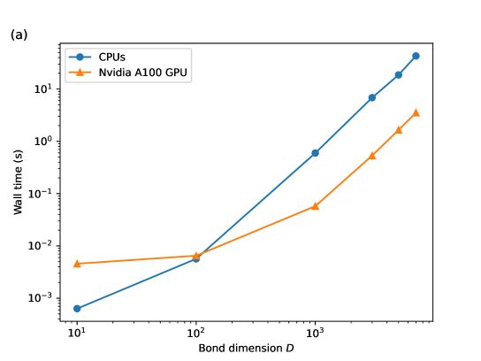
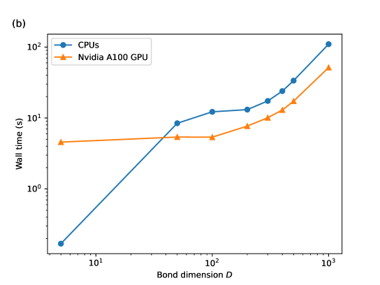
We next benchmark the performance of Cyntx and ITensor on GPU. The tests are executed on a machine with an AMD EPYC 7742 processor and a NVIDIA A100 GPU with 40GB memory. For the CPU runs, the parallelization is through the Intel MKL with 128 threads. Similar to the CPU benchmark, we test the performance of (a) the tensor contraction sketched in Fig. 17 and (b) the DMRG sweep. The benchmark results are shown in Fig. 19(a) and (b) respectively. In these benchmarks, one can observe a significant speedup for large bond dimensions when a GPU is used. The execution times for the tensor contraction show a 11 speedup can be reached for large bond dimensions. For a single iteration of an DMRG update, we gain a 2-3 speedup for large bond dimensions.
Summarizing, we conclude that Cytnx has a similar performance as ITensor. Cytnx allows users to run the most computationally expensive tasks on a GPU without much changes in the code by the user. This can reduce the computational time significantly.
12 Summary
We presented a library designed for high-dimensional tensor network algorithms. This library provides an easy-to-learn framework for new users to start developing their first tensor network code in a short period of time, yet comes with all the bells and whistles for advanced algorithms. This way, applications can quickly and conveniently be implemented and tested, but also be improved and optimized in a later step if desired. By design, the Cytnx Python and C++ interfaces follow the conventions in popular libraries for an intuitive usage. With almost identical APIs, users can easily switch between Python and C++ codes. As a benchmark, we compare typical tensor network operations against ITensor and obtain similar performance. Following a similiar syntax as in PyTorch, users can benefit from GPU acceleration with only minimal changes of their code. In our benchmark, a significant boost of the performance can be achieved when tensor operations are executed on a GPU.
There are several future directions for Cytnx. On the technical side, tensor network algorithms are often described as tensor diagrams, therefore a GUI interface that can automatically generate code from a tensor diagram, similar to TensorTrace [56], will be helpful. Also, automatic differentiation has become an important tool for tensor network computations [57, 58, 59, 60]. In the near future, Cytnx will support automatic differentiation through a PyTorch backend.
Many physics problems involve fermions. In these cases, exchanging the order of two particles results in a sign flip because of the anti-commutation relation between fermionic operators. In tensor network algorithms, this can be implemented with symmetric tensors and specific tensors called swap-gates, which produce the correct sign changes [61, 62]. An alternative approach uses Grassman tensors [63, 64]. In the future, an automated way to easily simulate fermionic systems will be implemented.
Currently, Cytnx supports only Abelian symmetries. With the current framework, it is easy to extend Cytnx to include symmetric UniTensors with more complicated symmetries such as SU(2). This is planned for a future version.
Regarding applications, several high-level tensor network algorithms such as (i)DMRG and iTEBD are implemented with Cytnx already [30]. We plan to extend this to provide a higher level abstraction in a spirit similar to the famous machine learning library Keras[65] so that physicists can focus on solving interesting physics problems. Through this, we hope to reduce the cognitive load for users and help develop more applications of tensor network algorithms in different fields of physics.
13 Acknowledgements
We would like to thank the National Center for High-Performance Computing (NCHC) and NVIDIA for providing us access to the NVIDIA A100 GPU. C.-M.C. acknowledges the support by the National Science and Technology Council (NSTC) under Grant No. 111-2112-M-110-006-MY3, and by the Yushan Young Scholar Program under the Ministry of Education (MOE) in Taiwan. We thank Yu-Cheng Lin and Shih-Hao Hung for their help on the implementation of the GPU functionalities of Cytnx.
Appendix A Tensor
A tensor is typically represented in Cytnx by a UniTensor object, which is explained in Sec. 5. In addition to the data of the tensor elements, a UniTensor object also contains meta information for bonds, labels, name, and symmetries. Internally, the data of a UniTensor is represented by one or more blocks. Each block contains a Tensor object, which is is a multi-dimensional array containing the values of the tensor. All elements belong to the same datatype. The behavior and the API of Tensor in Cytnx are very similar to the tensor in PyTorch and the array in NumPy. Typically, users do not have to deal with Tensor objects and we recommend the users to use UniTensor instead. However, we explain the underlying structure of a Tensor for advanced users here. A more extensive description can be found in the User Guide [30].
Creating a Tensor.
One can create a Tensor through generators such as zero, arange, ones:
Moreover, one can create a randomly initialized Tensor:
Data types.
The default data type of the elements in a Tensor is double in C++ and float in Python. One can create a Tensor with a different data type by providing an additional argument in the initialization function. It is possible to convert a Tensor of one data type to a different data type via Tensor.astype. The following example shows how to create a Tensor with dtype=Type.Int64 and convert the data type to Type.Double:
Reshaping.
The indices of a tensor can be combined or split, or brought in any other form of indices that match with the number of elements of the tensor. For this, the method reshape can be used on a Tensor. Suppose we want to create a rank-3 Tensor with shape=(2,3,4). We can start with a rank-1 Tensor with shape=(24) initialized using arange, and then reshape it to the desired shape. This can be done by using the Tensor.reshape function. Note that calling Tensor.reshape returns a new Tensor object, and the shape of the original Tensor object does not change. If one wants to change the shape of the original Tensor, one should use Tensor.reshape_.
Permutation.
If the order of indices shall be changed, one can call permute. Consider a rank-3 Tensor with shape=(2,3,4) as an example. This time we want to permute the order of the Tensor indices from (0,1,2) to (1,2,0). This can be achieved with Tensor.permute:
Converting to/from a NumPy array.
A Tensor can be converted to an NumPy array, (see also Sec. 5.8).
A conversion from NumPy to Cytnx Tensor is possible similarly:
Linear Algebra.
Cytnx provides several tensor operations and linear algebra functions like SVD, QR- and eigenvalue decomposition. These are explained in Sec. 9 for UniTensor objects, but can be used in a similar way for a Tensor. However, since a Tensor has no attribute rowrank, one has to permute and reshape the tensor to bring it into the form of a matrix before calling linear algebra functions that expect matrices as input. See the User Guide [39] for a list of supported operations and more details.
Device.
As explained in Sec. 10, tensors can be stored either in the CPU or GPU memory. If tensors are located on the GPU, one can directly make use of the parallelization and speed up the code execution. The APIs of tensor operations and linear algebra functions work the same way independently of where the tensors are stored. The code examples in LABEL:code:GPU_Tensor_declare and LABEL:code:TensorGPU demonstrate how to initialize a Tensor on a specific device and how to move a Tensor between devices.
Appendix B Advanced usage of Cytnx
Contiguous.
Here, we explain a more subtle behavior in permuting index order. In Cytnx, the permute operation does not move the elements in the memory immediately. Only the meta-data is changed. Permuting the index order means relocating the data in memory, which requires copying all the data in a Tensor or UniTensor. This can be expensive when the tensor dimensions are large. Instead, we follow an approach that is commonly used, for example in NumPy.array and torch.tensor: When permute is used, the order of the data is not rearranged yet. The actual copying of data to the new layout in memory only happens when Tensor.contiguous or UniTensor.contiguous is called. With this design, one can permute the indices several times without significant costs in execution time, and call contiguous only before an actual calculation is used which depends on the order of the elements – for example, before a tensor contraction. In practice, users do not need to call the contiguous command by themselves, as it is automatically done by Cytnx when needed.
We can use UniTensor.is_contiguous or Tensor.is_contiguous to check if a tensor is in contiguous form. One can force the contiguous status by calling Tensor.contiguous or Tensor.contiguous_ (similarly for UniTensor). However, the user does typically not need to do this explicitly as Cytnx automatically brings tensors to contiguous form when necessary.
Storage.
Storage is the low-level container that handles the memory allocation and the transfer between different devices. The tensor elements of a Tensor object are stored inside a Storage object. Typically, users do not directly need to access this object, but it might be useful in special cases. A Storage object can be created in a similar way as a Tensor. Note that Storage does not have the concept of shape, and is similar to the std::vector in C++. The code below in LABEL:code:StorageCreate shows how to create a Storage with all elements set to zero, and how to change the data type. One can call Storage.astype to convert between different data types, similar to the conversion of a Tensor. For details and available data types, see Appendix A.
Internally, the data of a Tensor is stored in a Storage object. We can get the Storage of a Tensor using Tensor.storage:
When a Tensor is non-contiguous (see Appendix B), its meta-data is detached from its memory. The latter is handled by a Storage. Consequently, calling Tensor.storage returns its current memory layout, not the permuted order of the Tensor. The following code example demonstrates this behavior:
OpenMP.
If OpenMP is available, Cytnx uses it for the parallel execution of code on CPUs. If Cytnx is compiled without OpenMP, Device.Ncpus (see Sec. 10.1) is always 1. If OpenMP is enabled, one can change the environment variable OMP_NUM_THREADS before executing the program to set a restriction on how many threads the program can use. For example, the following code example makes OpenMP and the internal functions of Cytnx use threads where possible:
The speedup when using OpenMP and eight threads instead of only one thread can be seen in the benchmark in Fig. 18.
References
- [1] R. Orús, A practical introduction to tensor networks: Matrix product states and projected entangled pair states, Annals of Physics 349, 117 (2014), 10.1016/j.aop.2014.06.013.
- [2] U. Schollwöck, The density-matrix renormalization group in the age of matrix product states, Annals of Physics 326(1), 96 (2011), 10.1016/j.aop.2010.09.012, January 2011 Special Issue.
- [3] J. I. Cirac, D. Pérez-García, N. Schuch and F. Verstraete, Matrix product states and projected entangled pair states: Concepts, symmetries, theorems, Rev. Mod. Phys. 93, 045003 (2021), 10.1103/RevModPhys.93.045003.
- [4] F. Verstraete, T. Nishino, U. Schollwöck, M. C. Bañuls, G. K. Chan and M. E. Stoudenmire, Density matrix renormalization group, 30 years on, Nature Reviews Physics 5(5), 273 (2023), 10.1038/s42254-023-00572-5.
- [5] H. Fehske, R. Schneider and A. Weiße, Computational Many-Particle Physics, Lecture Notes in Physics. Springer Berlin, Heidelberg, ISBN 978-3-540-74685-0,978-3-642-09414-9,978-3-540-74686-7, 10.1007/978-3-540-74686-7 (2008).
- [6] R. Orús, Tensor networks for complex quantum systems, Nature Reviews Physics 1(9), 538 (2019), 10.1038/s42254-019-0086-7.
- [7] H. Weimer, A. Kshetrimayum and R. Orús, Simulation methods for open quantum many-body systems, Rev. Mod. Phys. 93, 015008 (2021), 10.1103/RevModPhys.93.015008.
- [8] I. P. McCulloch, From density-matrix renormalization group to matrix product states, Journal of Statistical Mechanics: Theory and Experiment 2007(10), P10014 (2007), 10.1088/1742-5468/2007/10/P10014.
- [9] G. K.-L. Chan and S. Sharma, The density matrix renormalization group in quantum chemistry, Annual Review of Physical Chemistry 62(1), 465 (2011), 10.1146/annurev-physchem-032210-103338, PMID: 21219144.
- [10] G. K.-L. Chan, A. Keselman, N. Nakatani, Z. Li and S. R. White, Matrix product operators, matrix product states, and ab initio density matrix renormalization group algorithms, arXiv e-prints arXiv:1605.02611 (2016), 10.48550/arXiv.1605.02611.
- [11] K. H. Marti and M. Reiher, The density matrix renormalization group algorithm in quantum chemistry, Zeitschrift für Physikalische Chemie 224(3-4), 583 (2010), 10.1524/zpch.2010.6125.
- [12] G. K.-L. Chan, A. Keselman, N. Nakatani, Z. Li and S. R. White, Matrix product operators, matrix product states, and ab initio density matrix renormalization group algorithms, The Journal of Chemical Physics 145(1), 014102 (2016), 10.1063/1.4955108.
- [13] A. Baiardi and M. Reiher, The density matrix renormalization group in chemistry and molecular physics: Recent developments and new challenges, The Journal of Chemical Physics 152(4), 040903 (2020), 10.1063/1.5129672.
- [14] L. Freitag and M. Reiher, The Density Matrix Renormalization Group for Strong Correlation in Ground and Excited States, chap. 7, pp. 205–245, John Wiley & Sons, Ltd, ISBN 9781119417774, 10.1002/9781119417774.ch7 (2020).
- [15] Y. Cheng, Z. Xie and H. Ma, Post-density matrix renormalization group methods for describing dynamic electron correlation with large active spaces, The Journal of Physical Chemistry Letters 13(3), 904 (2022), 10.1021/acs.jpclett.1c04078.
- [16] M. C. Bañuls and K. Cichy, Review on novel methods for lattice gauge theories, Reports on Progress in Physics 83(2), 024401 (2020), 10.1088/1361-6633/ab6311.
- [17] Y. Meurice, R. Sakai and J. Unmuth-Yockey, Tensor lattice field theory for renormalization and quantum computing, Rev. Mod. Phys. 94, 025005 (2022), 10.1103/RevModPhys.94.025005.
- [18] M. Dalmonte and S. Montangero, Lattice gauge theory simulations in the quantum information era, Contemporary Physics 57(3), 388 (2016), 10.1080/00107514.2016.1151199.
- [19] M. C. Bañuls, R. Blatt, J. Catani, A. Celi, J. I. Cirac, M. Dalmonte, L. Fallani, K. Jansen, M. Lewenstein, S. Montangero, C. A. Muschik, B. Reznik et al., Simulating lattice gauge theories within quantum technologies, The European Physical Journal D 74(8), 165 (2020), 10.1140/epjd/e2020-100571-8.
- [20] E. Stoudenmire and D. J. Schwab, Supervised learning with tensor networks, In D. Lee, M. Sugiyama, U. Luxburg, I. Guyon and R. Garnett, eds., Advances in Neural Information Processing Systems, vol. 29. Curran Associates, Inc., https://proceedings.neurips.cc/paper_files/paper/2016/file/5314b9674c86e3f9d1ba25ef9bb32895-Paper.pdf (2016).
- [21] J. Liu, S. Li, J. Zhang and P. Zhang, Tensor networks for unsupervised machine learning, Phys. Rev. E 107, L012103 (2023), 10.1103/PhysRevE.107.L012103.
- [22] S. Y.-C. Chen, C.-M. Huang, C.-W. Hsing and Y.-J. Kao, An end-to-end trainable hybrid classical-quantum classifier, Machine Learning: Science and Technology 2(4), 045021 (2021), 10.1088/2632-2153/ac104d.
- [23] S. Y.-C. Chen, C.-M. Huang, C.-W. Hsing, H.-S. Goan and Y.-J. Kao, Variational quantum reinforcement learning via evolutionary optimization, Machine Learning: Science and Technology 3(1), 015025 (2022), 10.1088/2632-2153/ac4559.
- [24] M. Kiffner and D. Jaksch, Tensor network reduced order models for wall-bounded flows, arXiv e-prints arXiv:2303.03010 (2023), 10.48550/arXiv.2303.03010.
- [25] R. D. Peddinti, S. Pisoni, A. Marini, P. Lott, H. Argentieri, E. Tiunov and L. Aolita, Complete quantum-inspired framework for computational fluid dynamics, arXiv e-prints arXiv:2308.12972 (2023), 10.48550/arxiv.2308.12972.
- [26] H.-J. Liao, K. Wang, Z.-S. Zhou, P. Zhang and T. Xiang, Simulation of ibm’s kicked ising experiment with projected entangled pair operator, arXiv e-prints arXiv:2308.03082 (2023), 10.48550/arXiv.2308.03082.
- [27] T. Begušić and G. K.-L. Chan, Fast classical simulation of evidence for the utility of quantum computing before fault tolerance, arXiv e-prints arXiv:2306.16372 (2023), 10.48550/arXiv.2306.16372.
- [28] J. Tindall, M. Fishman, M. Stoudenmire and D. Sels, Efficient tensor network simulation of ibm’s eagle kicked ising experiment, arXiv e-prints arXiv:2306.14887 (2023), 10.48550/arXiv.2306.14887.
- [29] Cytnx, Github repository, https://github.com/kaihsin/Cytnx.
- [30] Cytnx, documentation and user guide, https://kaihsinwu.gitlab.io/Cytnx_doc/Intro.html.
- [31] M. Fishman, S. R. White and E. M. Stoudenmire, The ITensor Software Library for Tensor Network Calculations, SciPost Phys. Codebases p. 4 (2022), 10.21468/SciPostPhysCodeb.4.
- [32] Y. Motoyama, T. Okubo, K. Yoshimi, S. Morita, T. Kato and N. Kawashima, Tenes: Tensor network solver for quantum lattice systems, Computer Physics Communications 279, 108437 (2022), 10.1016/j.cpc.2022.108437.
- [33] J. Hauschild and F. Pollmann, Efficient numerical simulations with Tensor Networks: Tensor Network Python (TeNPy), SciPost Phys. Lect. Notes p. 5 (2018), 10.21468/SciPostPhysLectNotes.5.
- [34] SyTen, tensor library, https://syten.eu/docs/.
- [35] C. Roberts, A. Milsted, M. Ganahl, A. Zalcman, B. Fontaine, Y. Zou, J. Hidary, G. Vidal and S. Leichenauer, Tensornetwork: A library for physics and machine learning, arXiv e-prints arXiv:1905.01330 (2019), 10.48550/arXiv.1905.01330.
- [36] J. Haegeman, Tensorkit.jl, https://jutho.github.io/TensorKit.jl.
- [37] J. Gray, quimb: a python library for quantum information and many-body calculations, Journal of Open Source Software 3(29), 819 (2018), 10.21105/joss.00819.
- [38] Cytnx, API documentation, https://kaihsinwu.gitlab.io/cytnx_api/.
- [39] Cytnx, documentation and user guide, Section Linear algebra, https://kaihsinwu.gitlab.io/Cytnx_doc/guide/linalg.html.
- [40] B. Pirvu, V. Murg, J. I. Cirac and F. Verstraete, Matrix product operator representations, New Journal of Physics 12(2), 025012 (2010), 10.1088/1367-2630/12/2/025012.
- [41] S. Singh, R. N. C. Pfeifer and G. Vidal, Tensor network states and algorithms in the presence of a global u(1) symmetry, Phys. Rev. B 83, 115125 (2011), 10.1103/PhysRevB.83.115125.
- [42] S. Singh, R. N. C. Pfeifer and G. Vidal, Tensor network decompositions in the presence of a global symmetry, Phys. Rev. A 82, 050301 (2010), 10.1103/PhysRevA.82.050301.
- [43] S. Singh and G. Vidal, Tensor network states and algorithms in the presence of a global su(2) symmetry, Phys. Rev. B 86, 195114 (2012), 10.1103/PhysRevB.86.195114.
- [44] T. Nishino and K. Okunishi, Corner transfer matrix renormalization group method, Journal of the Physical Society of Japan 65(4), 891 (1996), 10.1143/JPSJ.65.891.
- [45] M. T. Fishman, L. Vanderstraeten, V. Zauner-Stauber, J. Haegeman and F. Verstraete, Faster methods for contracting infinite two-dimensional tensor networks, Phys. Rev. B 98, 235148 (2018), 10.1103/PhysRevB.98.235148.
- [46] F. Verstraete and J. I. Cirac, Renormalization algorithms for quantum-many body systems in two and higher dimensions, arXiv e-prints cond-mat/0407066 (2004), 10.48550/arXiv.cond-mat/0407066.
- [47] M. Schneider, J. Ostmeyer, K. Jansen, T. Luu and C. Urbach, Simulating both parity sectors of the hubbard model with tensor networks, Phys. Rev. B 104, 155118 (2021), 10.1103/PhysRevB.104.155118.
- [48] M. Schneider, The Hubbard model on a honeycomb lattice with fermionic tensor networks, Ph.D. thesis, Humboldt-Universität zu Berlin, Mathematisch-Naturwissenschaftliche Fakultät, 10.18452/25393 (2022).
- [49] Cytnx, documentation and user guide, Section Iterative Solver, https://kaihsinwu.gitlab.io/Cytnx_doc/guide/itersol.html.
- [50] S. Tomov, J. Dongarra and M. Baboulin, Towards dense linear algebra for hybrid GPU accelerated manycore systems, Parallel Computing 36(5-6), 232 (2010), 10.1016/j.parco.2009.12.005.
- [51] cuBLAS – Basic Linear Algebra on NVIDIA GPUs, https://developer.nvidia.com/cublas.
- [52] cuSOLVER – Direct Linear Solvers on NVIDIA GPUs, https://developer.nvidia.com/cusolver.
- [53] cuTENSOR – Tensor Linear Algebra on NVIDIA GPUs, https://developer.nvidia.com/cutensor.
- [54] cuQuantum – Accelerate quantum computing research., https://developer.nvidia.com/cublas.
- [55] S. R. White, Density matrix formulation for quantum renormalization groups, Phys. Rev. Lett. 69, 2863 (1992), 10.1103/PhysRevLett.69.2863.
- [56] G. Evenbly, Tensortrace: an application to contract tensor networks, 10.48550/arXiv.1911.02558 (2019).
- [57] H.-J. Liao, J.-G. Liu, L. Wang and T. Xiang, Differentiable programming tensor networks, Phys. Rev. X 9, 031041 (2019), 10.1103/PhysRevX.9.031041.
- [58] J. Hasik, D. Poilblanc and F. Becca, Investigation of the Néel phase of the frustrated Heisenberg antiferromagnet by differentiable symmetric tensor networks, SciPost Phys. 10, 012 (2021), 10.21468/SciPostPhys.10.1.012.
- [59] J. Naumann, E. Lennart Weerda, M. Rizzi, J. Eisert and P. Schmoll, variPEPS – a versatile tensor network library for variational ground state simulations in two spatial dimensions, arXiv e-prints arXiv:2308.12358 (2023), 10.48550/arXiv.2308.12358.
- [60] A. Francuz, N. Schuch and B. Vanhecke, Stable and efficient differentiation of tensor network algorithms, arXiv e-prints arXiv:2311.11894 (2023), 10.48550/arXiv.2311.11894.
- [61] P. Corboz, R. Orús, B. Bauer and G. Vidal, Simulation of strongly correlated fermions in two spatial dimensions with fermionic projected entangled-pair states, Phys. Rev. B 81, 165104 (2010), 10.1103/PhysRevB.81.165104.
- [62] P. Corboz and G. Vidal, Fermionic multiscale entanglement renormalization ansatz, Phys. Rev. B 80, 165129 (2009), 10.1103/PhysRevB.80.165129.
- [63] Z.-C. Gu, Efficient simulation of grassmann tensor product states, Phys. Rev. B 88, 115139 (2013), 10.1103/PhysRevB.88.115139.
- [64] A. Yosprakob, GrassmannTN: A Python package for Grassmann tensor network computations, SciPost Phys. Codebases p. 20 (2023), 10.21468/SciPostPhysCodeb.20.
- [65] F. Chollet et al., Keras, https://github.com/fchollet/keras (2015).