Image Processing and Legendre Polynomials

E. Celeghini1    M. Gadella2    M. A. del Olmo2 1 Dipartimento di Fisica, Università di Firenze and INFN-Sezione di Firenze, I50019 Sesto Fiorentino, Firenze, Italy
2 Departamento de Física Teórica, Atómica y Optica and IMUVA, Universidad de Valladolid, 47011 Valladolid, Spain
enrico.celeghini@gmail.com, manuel.gadella1@gmail.com, marianoantonio.olmo@uva.es
Abstract

In this paper, we consider a basis of square integrable functions on a rectangle, contained in 2superscript2{\mathbb{R}}^{2}, constructed with Legendre polynomials, suitable for the analogical description of images on the plane. After extending the Legendre polynomials to any arbitrary interval of the form [a,b]𝑎𝑏[a,b], from its original form on [1,1]11[-1,1], we generalize the basis of Legendre polynomials to two dimensions. The extension to color images can be realized with the obvious procedure of considering togheter three monocromatic images and the extension to three (and more) dimensions is straighforward. We present some mathematical constructions such as Gelfand triples appropriate on this context. We compare the digital and analogical descriptions of the model.

preprint: AIP/123-QED

I Introduction and Motivation

Orthogonal polynomials and their generalizations are being widely used in many areas of the broad field of signal processing as we may see, for instance, in Ref. QZWZC23 ; JRM12 ; see2007 ; zhoushutoumoulin2005 ; huntmukundam2004 ; paramersranong2003 ; mukundamong2001 ; teague1980 ; hu1962 . In particular QZWZC23 contains an extensive list of additional references. Since the seminal paper by Teague in 1980 teague1980 , Legendre polynomials via Legendre moments have also been largely used mukundanramakrishnan1995 ; yapparamesran2005 ; chongraveendranmukundan2004 ; xiaowangli2014 ; YangMaMiaoLiuWangMeng2019 ; hosnydarwishaboelenen2020 .

As we know, we require a normalization in order to use a Hilbert space basis with Legendre polynomials szego2003 . This normalization is given by a multiplicative factor on the Legendre polynomials {Ln(x)}nsubscriptsubscript𝐿𝑛𝑥𝑛\{L_{n}(x)\}_{n\in{\mathbb{N}}}\, given by n+1/2𝑛12\sqrt{n+1/2} olmo2013 . By historical reasons related to trigonometry, Legendre polynomials are usually defined in the interval  [1,+1]11[-1,+1]. In fact, the original problem discussed by Legendre, which gave rise to these kind of polynomials showed spherical symmetry legendre1785 .

The scientific discussion contained in the present article has a motivation with roots on the signal theory and the theory of images. As the ultimate purpose would be the use of the above mentioned basis in the description of a set of data of a digital sample, it would be necessary to define these functions on a general compact interval such as [a,b]𝑎𝑏[a,b] (with a<b𝑎𝑏a<b), supporting the original data of the problem to be discussed.

The natural definition of Legendre polynomials on intervals of the form [a,b]𝑎𝑏[a,b]\subset{\mathbb{R}} are valid for data analysis in one dimension (1D). However, for 2D or 3D, we need to extend the notion of Legendre polynomials to these contexts. In these cases, as well as in the analysis of data from images, we need bases of functions supported on a 2D or 3D real subset, which are constructed using Lagrange polynomials and are addressed to the study of black and white images. In the case of color images we need to work in a higher dimensions, as we will see later.

Thus, let us start with bases of functions in 2D built with Lagrange polynomials, which are the normalized versions of {Lm(x)Ln(y)}m,nsubscripttensor-productsubscript𝐿𝑚𝑥subscript𝐿𝑛𝑦𝑚𝑛\{L_{m}(x)\otimes L_{n}(y)\}_{m,n\in{\mathbb{N}}}, with x[ax,bx]𝑥subscript𝑎𝑥subscript𝑏𝑥x\in[a_{x},b_{x}]\subset{\mathbb{R}} and y[ay,by]𝑦subscript𝑎𝑦subscript𝑏𝑦y\in[a_{y},b_{y}]\subset{\mathbb{R}}. In a digital description the informations given to construct a black and white image can be given by a set of three real parameters {[s]k1,k2}subscriptdelimited-[]𝑠subscript𝑘1subscript𝑘2\{[s]_{k_{1},k_{2}}\}. Here 0<s<10𝑠10<s<1 gives the saturation of black at the point (k1,k2)subscript𝑘1subscript𝑘2(k_{1},k_{2}) in the image, or the intensity or gray level of the image at that point. On the contrary, in terms of the presented analogical description, the saturation of the black is given by a term like that dm,nLm(x)Ln(y)tensor-productsubscript𝑑𝑚𝑛subscript𝐿𝑚𝑥subscript𝐿𝑛𝑦\sum d_{m,n}\,L_{m}(x)\otimes L_{n}(y). The fundamental difference between the two descriptions is that the coefficients {dm,n}subscript𝑑𝑚𝑛\{d_{m,n}\}, labelled by the natural parameters m,n𝑚𝑛m,n\in{\mathbb{N}}, are related to the level of saturation of the black on the whole image and not just at a given point. However, the evaluation of information in a digital image is far from satisfactory for a human being, since our brain is not able to analyze the Gestalt of a too complex image century1 ; century2 .

Thus, the motivation of this paper has been, in principle, analogical also if in our society the attention is mainly addressed to the digital world as the signals in computer science, as well as in our eyes, are indeed discrete. However, the human brain is not able to understand the information contained in a signal where too many pixels are independent. In fact, we read one image of many scattered pixels of similar grey as an homogeneous surface. Consequently, a human being can interpret only a few images among the many given by a computer and are evaluated by the theory of information. Sometimes the information is extremely reduced because of the presence of many contiguous similar pixels. Thus, in order to communicate with humans, a computer must remove almost all the information contained in the signal at the final step of its analysis and the results have to be given in an analogical form.

Taking into account this point of view, we may say that the present paper deals with both digitalized and analogical images. Indeed, we intend to present an analogized approach based on Legendre polynomials to all images. There is a nice similarity between this procedure and the action of an ophthalmologist when prescribing the glasses to a patient: the ophthalmologist does not use a detailed analysis of the patient’s eyes. Instead, he or she just takes into account the few first coefficients of a series expansion in terms of Zernike functions zernike1934 ; celeghini2017 ; olmo2019 .

Another possible use of the analogical sum of generalized Legendre polynomials can be to subtract from a digital image the corresponding analogical one. In this way, we may enhance the details, since the analogical image is usually more smooth than the original. Nevertheless, this does not imply that all the machinery of digital images, such as the realization of a 2D image as a section of multi-dimensional data, could not be used by the human operator before the final presentation.

Along the present paper, we are taking into account several issues. First of all, we go through a detailed description of the 1D Legendre polynomials on a real interval of the form [a,b]𝑎𝑏[a,b]. Particular interest are those for which a=0𝑎0a=0, since the construction is related to the standard discrete numbering in computer science where the numbering of pixels starts from pixel 11{1} and finishes with pixel n𝑛{n}. Nevertheless, the use of intervals of the form [a,b]𝑎𝑏[a,b] have their applications to discrete image analysis, when one just considers a part of pixels in one given image.

In a second step, we intend to extend the analysis in 1D to 2D rectangular images on sets of the form [a1,b1][a2,b2]2tensor-productsubscript𝑎1subscript𝑏1subscript𝑎2subscript𝑏2superscript2[a_{1},b_{1}]\otimes[a_{2},b_{2}]\subset{\mathbb{R}}^{2}, where the involved parameters are, in principle, arbitrary albeit finite. The aim goes to the description of a rectangular black and white image. Here, the saturation of the black at each point (x,y)𝑥𝑦(x,y) is given by

f(x,y)=n1,n2dn1,n2Wn1(ax,bx,x)Wn2(ay,by,y),𝑓𝑥𝑦subscriptsubscript𝑛1subscript𝑛2tensor-productsubscript𝑑subscript𝑛1subscript𝑛2subscript𝑊subscript𝑛1subscript𝑎𝑥subscript𝑏𝑥𝑥subscript𝑊subscript𝑛2subscript𝑎𝑦subscript𝑏𝑦𝑦f(x,y)\,=\,\sum_{n_{1},n_{2}}\;d_{n_{1},n_{2}}\;\;W_{n_{1}}(a_{x},b_{x},x)\otimes W_{n_{2}}(a_{y},b_{y},y)\,, (1)

where {Wn(a,b,x)}subscript𝑊𝑛𝑎𝑏𝑥\{W_{n}(a,b,x)\} gives the generalization of the Legendre polynomials as functions supported on a compact interval of the form [a,b]𝑎𝑏[a,b]. Consequently, the tensor products Wn1(ax,bx,x)Wn2(ay,by,y)tensor-productsubscript𝑊subscript𝑛1subscript𝑎𝑥subscript𝑏𝑥𝑥subscript𝑊subscript𝑛2subscript𝑎𝑦subscript𝑏𝑦𝑦W_{n_{1}}(a_{x},b_{x},x)\otimes W_{n_{2}}(a_{y},b_{y},y) give the extension of these functions to the 2D rectangle [ax,bx][ay,by]tensor-productsubscript𝑎𝑥subscript𝑏𝑥subscript𝑎𝑦subscript𝑏𝑦[a_{x},b_{x}]\otimes[a_{y},b_{y}].

In order to represent trichrome images, we need the product of three ‘black and white’ images that may be given as a product of three functions of the form (1) as

fR(x,y)fG(x,y)fB(x,y).tensor-producttensor-productsubscript𝑓𝑅𝑥𝑦subscript𝑓𝐺𝑥𝑦subscript𝑓𝐵𝑥𝑦f_{R}(x,y)\;\otimes f_{G}(x,y)\;\otimes f_{B}(x,y)\,. (2)

Here, fR(x,y),fG(x,y)subscript𝑓𝑅𝑥𝑦subscript𝑓𝐺𝑥𝑦f_{R}(x,y),f_{G}(x,y) and fB(x,y)subscript𝑓𝐵𝑥𝑦f_{B}(x,y) are the Red, Green and Blue components of color image as supposed to be the primary colors. Some of these ideas has been proposed in olmo2019 ; CGO22 .

The central structure accommodating the functions for rectangular black and white images is the Hilbert space L2([ax,bx][ay,by])superscript𝐿2tensor-productsubscript𝑎𝑥subscript𝑏𝑥subscript𝑎𝑦subscript𝑏𝑦L^{2}([a_{x},b_{x}]\otimes[a_{y},b_{y}]). Nevertheless, equipations of Hilbert spaces such as Gelfand triplets GEL are often important so as to provide subspaces in which observables are continuous operators. Gelfand triplets or rigged Hilbert spaces (RHS) are a sequence of three infinite dimensional vector spaces,

ΦΦ×,ΦsuperscriptΦ\Phi\subset\mathcal{H}\subset\Phi^{\times}\,, (3)

where \mathcal{H} is a separable infinite dimensional complex Hilbert space, ΦΦ\Phi is a dense subspace endowed with a locally convex topology finer than the Hilbert space topology. Finally, Φ×superscriptΦ\Phi^{\times} is the dual space of ΦΦ\Phi, usually endowed with a topology compatible with the dual pair {Φ,Φ×}ΦsuperscriptΦ\{\Phi,\Phi^{\times}\}, normally the strong or weak topology. Gelfand triplets has many applications either in mathematics or theoretical physics. Due to the wide range of these applications, we only mention here the mathematical formalization of the Dirac formalism of Quantum Mechanics ROB ; ANT ; MEL ; BOH ; GG and the signal processing olmo2016 .

This paper is organized as follows: In Section  II, we revise some features on orthogonal polynomials and their use as basis of square integrable functions on the real line or real intervals olmo2016 . In Section III, we derive the definition of Legendre polynomials on an arbitrary compact interval [a,b],a<b𝑎𝑏𝑎𝑏[a,b],a<b, starting from the usual definition on [1,1]11[-1,1]. These are the so called generalized Legendre polynomials, Wn(a,b,x)Wn[a,b](x)subscript𝑊𝑛𝑎𝑏𝑥subscriptsuperscript𝑊𝑎𝑏𝑛𝑥W_{n}(a,b,x)\equiv W^{[a,b]}_{n}(x). We show that they have similar properties than the standard Legendre polynomials Ln(x)subscript𝐿𝑛𝑥L_{n}(x). In Section IV we show that the generalized Legendre polynomials Wn[a,b](x)subscriptsuperscript𝑊𝑎𝑏𝑛𝑥W^{[a,b]}_{n}(x), in complete analogy with the usual Legendre polynomials Ln(x)subscript𝐿𝑛𝑥L_{n}(x), for any pair of real numbers a,b𝑎𝑏a,b (a<b)𝑎𝑏(a<b) are a unitary irreducible representation (UIR) of the group SU(1,1)𝑆𝑈11SU(1,1) with Casimir 𝒞=1/4𝒞14{\cal C}=-1/4. A generalization of Legendre polynomials on n-dimensional (nD) rctangles appears in Section V. The construction of Gelfand triplets suitable for our particular type of problem is left to Section VI where the continuity is proved. The paper closes with few concluding remarks.

II Bases on the Real Line and Orthogonal Polynomials

To begin with, let us consider orthogonal polynomials defined on real intervals of the form [a,b]𝑎𝑏[a,b], either finite or infinite, i.e., a<b+𝑎𝑏-\infty\leq a<b\leq+\infty cambanis . One standard procedure described in Quantum Mechanics textbooks comes after the association of, in general almost all x[a,b]𝑥𝑎𝑏x\in[a,b] with respect to some measure, a generalized vector, |xket𝑥|x\rangle, outside the Hilbert space, although in the dual Φ×superscriptΦ\Phi^{\times} of a Gelfand triplet (RHS) of the form given in (3). Constructions of this kind come after the celebrated Gelfand-Maurin theorem GEL ; ROB ; ANT ; MEL ; GG1 ; GG2 , which we do not discuss it in here. These generalized vectors form a generalized basis, which plays an interesting role on the discussion in the sequel.

In most of examples studied so far olmo2016 ; olmo2019 ; CGO22 ; CGO20 , we have the similar structure: an infinite dimensional separable Hilbert space Ea,bsubscriptsubscript𝐸𝑎𝑏{\mathcal{H}}_{E_{a,b}} equipped as in (3), where Ea,b:=[a,b]assignsubscript𝐸𝑎𝑏𝑎𝑏E_{a,b}:=[a,b]\subset{\mathbb{R}}. To all (or almost all with respect to some measure) x[a,b]𝑥𝑎𝑏x\in[a,b], it corresponds a generalized vector on the dual, |xket𝑥|x\rangle (related to x|Φbra𝑥Φ\langle x|\in\Phi) see (3), fulfilling some formal properties of orthogonality and completeness, which are usually presented as, respectively,

x|y=δ(xy),ab|x𝑑xx|=𝕀,x,yEa,b.formulae-sequenceinner-product𝑥𝑦𝛿𝑥𝑦formulae-sequencesuperscriptsubscript𝑎𝑏ket𝑥differential-d𝑥bra𝑥𝕀for-all𝑥𝑦subscript𝐸𝑎𝑏\langle x|y\rangle=\delta(x-y)\,,\qquad\int_{a}^{b}|x\rangle dx\langle x|={\mathbb{I}}\,,\qquad\quad\;\forall\;x,y\;\in\,E_{a,b}\,. (4)

The abstract Hilbert space admits a representation L2(Ea,b)superscript𝐿2subscript𝐸𝑎𝑏{L}^{2}(E_{a,b}), where an orthonormal basis (complete orthonormal set) is a sequence of functions. In our examples, we have chosen bases of special functions {Fn(x)}nsubscriptsubscript𝐹𝑛𝑥𝑛\{F_{n}(x)\}_{n\in{\mathbb{N}}} for which the orthonormality and completeness relations read, respectively, as

abFn(x)Fm(x)𝑑x=δn,m,n=0Fn(x)Fn(y)=δ(xy),x,yEa,b.formulae-sequencesuperscriptsubscript𝑎𝑏subscript𝐹𝑛𝑥subscript𝐹𝑚𝑥differential-d𝑥subscript𝛿𝑛𝑚formulae-sequencesuperscriptsubscript𝑛0subscript𝐹𝑛𝑥subscript𝐹𝑛𝑦𝛿𝑥𝑦for-all𝑥𝑦subscript𝐸𝑎𝑏\int_{a}^{b}\,F_{n}(x)\;F_{m}(x)\;dx\;=\,\delta_{n,m}\,,\qquad\sum_{n=0}^{\infty}\;F_{n}(x)\;F_{n}(y)\;=\;\delta(x-y)\,,\quad\;\forall\;x,y\in E_{a,b}\,. (5)

In each of our examples, we have constructed a Gelfand triple of the form

ΦEa,bL2(Ea,b)ΦEa,b×,subscriptΦsubscript𝐸𝑎𝑏superscript𝐿2subscript𝐸𝑎𝑏subscriptsuperscriptΦsubscript𝐸𝑎𝑏\Phi_{E_{a,b}}\subset L^{2}(E_{a,b})\subset\Phi^{\times}_{E_{a,b}}\,, (6)

such that Fn(x)ΦEa,bsubscript𝐹𝑛𝑥subscriptΦsubscript𝐸𝑎𝑏F_{n}(x)\in\Phi_{E_{a,b}}. We have shown that there exists a unitary operator, U:Ea,bL2(Ea,b):𝑈subscriptsubscript𝐸𝑎𝑏superscript𝐿2subscript𝐸𝑎𝑏U:{\mathcal{H}}_{E_{a,b}}\longmapsto{L}^{2}(E_{a,b}), not necessarily unique, such that if Φ=UΦEa,bΦ𝑈subscriptΦsubscript𝐸𝑎𝑏\Phi=U\Phi_{E_{a,b}}, then

ΦEa,bΦ×,Φsubscriptsubscript𝐸𝑎𝑏superscriptΦ\Phi\subset{\mathcal{H}}_{E_{a,b}}\subset\Phi^{\times}\,, (7)

is an abstract Gelfand triple with the property that {|x}xEa,bΦEa,b×subscriptket𝑥𝑥subscript𝐸𝑎𝑏subscriptsuperscriptΦsubscript𝐸𝑎𝑏\{|x\rangle\}_{x\in E_{a,b}}\subset\Phi^{\times}_{E_{a,b}}. Hereafter, we construct an orthonormal basis, {|n}nsubscriptket𝑛𝑛\{|n\rangle\}_{n\in{\mathbb{N}}} on the abstract Hilbert space Ea,bsubscriptsubscript𝐸𝑎𝑏{\mathcal{H}}_{E_{a,b}} such that |n:=UFnassignket𝑛𝑈subscript𝐹𝑛|n\rangle:=UF_{n}. It is shown that it satisfies the formal expression

|n:=ab|xFn(x)𝑑x.assignket𝑛superscriptsubscript𝑎𝑏ket𝑥subscript𝐹𝑛𝑥differential-d𝑥|n\rangle\,:=\int_{a}^{b}\;|x\rangle\;F_{n}(x)\;dx\,. (8)

Orthonormality and completeness relations for {|n}nsubscriptket𝑛𝑛\{|n\rangle\}_{n\in{\mathbb{N}}} are given by the following respective relations:

n|m=δn,m,n=0|nn|=𝕀,n,m,formulae-sequenceinner-product𝑛𝑚subscript𝛿𝑛𝑚formulae-sequencesuperscriptsubscript𝑛0ket𝑛bra𝑛𝕀for-all𝑛𝑚\langle n|m\rangle\;=\;\delta_{n,m}\,,\qquad\sum_{n=0}^{\infty}\;|n\rangle\langle n|\;=\;{\mathbb{I}}\,,\quad\forall\;n,m\in{\mathbb{N}}\,, (9)

where 𝕀𝕀\mathbb{I} is the identity on Ea,bsubscriptsubscript𝐸𝑎𝑏{\mathcal{H}}_{E_{a,b}}.

In terms of the generalized vectors {|x}xEa,bsubscriptket𝑥𝑥subscript𝐸𝑎𝑏\{|x\rangle\}_{x\in E_{a,b}} and the orthonormal basis {|n}nsubscriptket𝑛𝑛\{|n\rangle\}_{n\in{\mathbb{N}}}, we may write the functions {Fn(x)}nsubscriptsubscript𝐹𝑛𝑥𝑛\{F_{n}(x)\}_{n\in{\mathbb{N}}}, assumed to be real, as

Fn(x):=x|n=n|x.assignsubscript𝐹𝑛𝑥inner-product𝑥𝑛inner-product𝑛𝑥F_{n}(x)\;:=\;\langle x|n\rangle\;=\;\langle n|x\rangle\,. (10)

An arbitrary vector |fΦEa,bket𝑓subscriptΦsubscript𝐸𝑎𝑏|f\rangle\in\Phi_{E_{a,b}} can also be expressed in terms of both, the orthonormal basis {|n}nsubscriptket𝑛𝑛\{|n\rangle\}_{n\in{\mathbb{N}}} as well as in the set of generalized vectors {|x}xEa,bsubscriptket𝑥𝑥subscript𝐸𝑎𝑏\{|x\rangle\}_{x\in E_{a,b}} in the following way:

|f=ab|x𝑑xx|f=n=0|nn|f.ket𝑓superscriptsubscript𝑎𝑏ket𝑥differential-d𝑥inner-product𝑥𝑓superscriptsubscript𝑛0ket𝑛inner-product𝑛𝑓|f\rangle\;=\;\int_{a}^{b}\;|x\rangle\,dx\,\langle x|f\rangle\;\;=\;\sum_{n=0}^{\infty}\;|n\rangle\;\langle n|f\rangle\,. (11)

From this point of view, we may assert that the set {|x}x[a,b]subscriptket𝑥𝑥𝑎𝑏\{|x\rangle\}_{x\in[a,b]} form a generalized continuous basis for all vectors |fΦEa,bket𝑓subscriptΦsubscript𝐸𝑎𝑏|f\rangle\in\Phi_{E_{a,b}}. Also, any function f(x)Φ𝑓𝑥Φf(x)\in\Phi, with f(x)=U|f𝑓𝑥𝑈ket𝑓f(x)=U|f\rangle can be written as follows:

f(x)=x|f=n=0fnFn(x),fn=n|f=abf(x)Fn(x)𝑑x.formulae-sequence𝑓𝑥inner-product𝑥𝑓superscriptsubscript𝑛0subscript𝑓𝑛subscript𝐹𝑛𝑥subscript𝑓𝑛inner-product𝑛𝑓superscriptsubscript𝑎𝑏𝑓𝑥subscript𝐹𝑛𝑥differential-d𝑥f(x)=\;\langle x|f\rangle\,=\,\sum_{n=0}^{\infty}f_{n}\;F_{n}(x)\,,\qquad f_{n}\,=\,\langle n|f\rangle\,=\,\int_{a}^{b}\,f(x)\;F_{n}(x)\;dx\,. (12)

Obviously, the {fn}nsubscriptsubscript𝑓𝑛𝑛\{f_{n}\}_{n\in{\mathbb{N}}} is the set of coefficients of the span of any f(x)Φ𝑓𝑥Φf(x)\in\Phi in terms of the given orthonormal basis. This means that

g|f=n=0gnfn=abg(x)f(x)𝑑x,n=0|fn|2=ab|f(x)|2𝑑x.formulae-sequenceinner-product𝑔𝑓superscriptsubscript𝑛0superscriptsubscript𝑔𝑛subscript𝑓𝑛superscriptsubscript𝑎𝑏superscript𝑔𝑥𝑓𝑥differential-d𝑥superscriptsubscript𝑛0superscriptsubscript𝑓𝑛2superscriptsubscript𝑎𝑏superscript𝑓𝑥2differential-d𝑥\langle g|f\rangle\;=\,\sum_{n=0}^{\infty}\;g_{n}^{*}\cdot f_{n}\;=\;\int_{a}^{b}g^{*}(x)\cdot f(x)dx\,,\qquad\sum_{n=0}^{\infty}|f_{n}|^{2}\;=\,\int_{a}^{b}|f(x)|^{2}dx\,. (13)

As we have remarked earlier, we use normalized orthogonal polynomials as orthonormal bases on L2(Ea,b)superscript𝐿2subscript𝐸𝑎𝑏L^{2}(E_{a,b}). In this sense, we have shown that Gelfand triplets or RHS are the suitable setting that give meaning to formulas including special functions, generalized vectors, generalized eigenvalues of operators and discrete orthonormal and continuous bases. Moreover, it allows for representations of Lie algebras of symmetries of physical systems, as continuous operators on a locally convex space contained on their domain. Needless to say that the type of basis of special functions depends, among other considerations, of the kind of interval [a,b]𝑎𝑏[a,b] used. Here, there are some examples szego2003 ; OLBC2010 ; olmo2013 :

2.1) Assume that a=𝑎a=-\infty, b=+𝑏b=+\infty, i.e., <x<𝑥-\infty<x<\infty. The Hilbert space L2(Ea,b)superscript𝐿2subscript𝐸𝑎𝑏{L}^{2}(E_{a,b}) is L2()superscript𝐿2L^{2}({\mathbb{R}}). An orthonormal basis on L2()superscript𝐿2L^{2}({\mathbb{R}}) is given by the normalized Hermite functions, {Kn(x)}nsubscriptsubscript𝐾𝑛𝑥𝑛\{K_{n}(x)\}_{n\in{\mathbb{N}}}, defined as

Kn(x):=ex2/22nn!πHn(x),n,n=0,1,2,,formulae-sequenceassignsubscript𝐾𝑛𝑥superscript𝑒superscript𝑥22superscript2𝑛𝑛𝜋subscript𝐻𝑛𝑥formulae-sequence𝑛𝑛012K_{n}(x):=\;\;\frac{e^{-x^{2}/2}}{\sqrt{2^{n}\,n!\sqrt{\pi}}}\;\;H_{n}(x)\,,\qquad n\in{\mathbb{N}}\,,\qquad n=0,1,2,\dots\,, (14)

where {Hn(x)}nsubscriptsubscript𝐻𝑛𝑥𝑛\{H_{n}(x)\}_{n\in{\mathbb{N}}} are the Hermite polynomials. For an unbounded interval, our special functions are products of some polynomials times a regularization function, in our case a gaussian, times a normalization constant. A typical equippation of L2()superscript𝐿2L^{2}({\mathbb{R}}) is given by 𝒮L2()𝒮×𝒮superscript𝐿2superscript𝒮\mathcal{S}\subset L^{2}({\mathbb{R}})\subset\mathcal{S}^{\times}, where 𝒮𝒮\mathcal{S} is the Schwartz space simon1980 , which contains all Hermite functions, and 𝒮×superscript𝒮\mathcal{S}^{\times} is the space of tempered distributions.

2.2) Now, take, a=0𝑎0a=0 and b=+𝑏b=+\infty, so that L2(Ea,b)L2(+)superscript𝐿2subscript𝐸𝑎𝑏superscript𝐿2superscript{L}^{2}(E_{a,b})\equiv L^{2}({\mathbb{R}}^{+}). An orthonormal basis is given by the Laguerre functions, which are products of Laguerre polynomials times a negative exponential:

Mn(x):=ex/2Ln(x),n,x[0,+)+.formulae-sequenceassignsubscript𝑀𝑛𝑥superscript𝑒𝑥2subscript𝐿𝑛𝑥formulae-sequence𝑛𝑥0superscriptM_{n}(x):=e^{-x/2}\;{L}_{n}(x),\qquad n\in{\mathbb{N}}\,,\;x\in[0,+\infty)\equiv{\mathbb{R}}^{+}\,. (15)

2.3) If a=1𝑎1a=-1 and b=1𝑏1b=1, we have the Hilbert space L2[1,1]superscript𝐿211L^{2}[-1,1], where the normalized Legendre polynomials form an orthonormal basis.

III Legendre polynomials and their generalization

The Legendre polynomials,

Pn(x):=12nn!dndxn(x21)n,assignsubscript𝑃𝑛𝑥1superscript2𝑛𝑛superscript𝑑𝑛𝑑superscript𝑥𝑛superscriptsuperscript𝑥21𝑛\ P_{n}(x):=\frac{1}{2^{n}\,n!}\,\frac{d^{n}}{dx^{n}}\,(x^{2}-1)^{n}\,, (16)

are defined on the interval [1,1]11[-1,1] and verify the following orthonormality and completeness relations:

11Pn(x)(n+1/2)Pm(x)𝑑x=δn,m,n=0Pn(x)(n+1/2)Pn(y)=δ(xy).formulae-sequencesuperscriptsubscript11subscript𝑃𝑛𝑥𝑛12subscript𝑃𝑚𝑥differential-d𝑥subscript𝛿𝑛𝑚superscriptsubscript𝑛0subscript𝑃𝑛𝑥𝑛12subscript𝑃𝑛𝑦𝛿𝑥𝑦\int_{-1}^{1}\,P_{n}(x)\,(n+1/2)\,P_{m}(x)\;dx\;=\,\delta_{n,m}\,,\qquad\sum_{n=0}^{\infty}\;P_{n}(x)\,(n+1/2)\,P_{n}(y)\;=\;\delta(x-y)\,. (17)

This means that the normalized Legendre polynomials (NLP) are

Kn(x):=n+1/2Pn(x).assignsubscript𝐾𝑛𝑥𝑛12subscript𝑃𝑛𝑥K_{n}(x):=\sqrt{n+1/2}\,\ P_{n}(x)\,. (18)

They are an orthonormal basis on L2[1,1]superscript𝐿211L^{2}[-1,1], the space of measurable square integrable complex functions on [1,1]11[-1,1]. From this, we may construct an orthonormal basis for L2[a,b]superscript𝐿2𝑎𝑏L^{2}[a,b] in terms of the functions Wn(a,b,x)subscript𝑊𝑛𝑎𝑏𝑥W_{n}(a,b,x), with a𝑎a and b𝑏b finite, as follows:

Wn(a,b,x):=2baKn(2xbab+aba),n,axb.formulae-sequenceassignsubscript𝑊𝑛𝑎𝑏𝑥2𝑏𝑎subscript𝐾𝑛2𝑥𝑏𝑎𝑏𝑎𝑏𝑎formulae-sequence𝑛𝑎𝑥𝑏W_{n}(a,b,x):=\sqrt{\frac{2}{b-a}}\;\;\;K_{n}\left(\frac{2x}{b-a}-\frac{b+a}{b-a}\right)\,,\qquad\;n\in{\mathbb{N}}\,,\;\;a\leq x\leq b\,. (19)

When ba=1(1)𝑏𝑎11b-a=1-(-1), i.e., the interval [a,b]𝑎𝑏[a,b] has the same width than [1,1]11[-1,1], the argument of Pn(x)subscript𝑃𝑛𝑥P_{n}(x) reduces to x(b+a)/2𝑥𝑏𝑎2x-(b+a)/2. Functions Wn(a,b,x)subscript𝑊𝑛𝑎𝑏𝑥W_{n}(a,b,x) are the generalized Legendre polynomials (GLP) on the interval [a,b]𝑎𝑏[a,b].

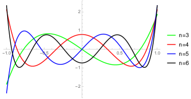
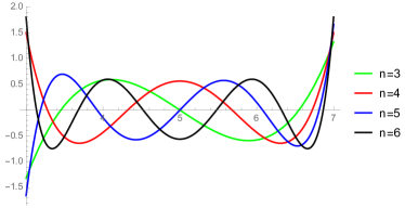
In Fig. 1.a the NLP Kn(x)subscript𝐾𝑛𝑥K_{n}(x) for different values of the label n𝑛n are represented and in Fig. 1.b appear the GLP Wn(a,b,x)subscript𝑊𝑛𝑎𝑏𝑥W_{n}(a,b,x) defined in the interval [3,7]37[3,7] also for some values of n𝑛n.

From the orthonormality and completeness relations satisfied by the orthonormal Legendre polynomials, we readily obtain similar relations for the new GLP, such that

abWn(a,b,x)Wm(a,b,x)𝑑x=δn,m,n=0Wn(a,b,x)Wn(a,b,y)=δ(xy),x,y[a,b].superscriptsubscript𝑎𝑏subscript𝑊𝑛𝑎𝑏𝑥subscript𝑊𝑚𝑎𝑏𝑥differential-d𝑥subscript𝛿𝑛𝑚superscriptsubscript𝑛0subscript𝑊𝑛𝑎𝑏𝑥subscript𝑊𝑛𝑎𝑏𝑦𝛿𝑥𝑦for-all𝑥𝑦𝑎𝑏\begin{array}[]{lll}\displaystyle\int_{a}^{b}W_{n}(a,b,x)\,W_{m}(a,b,x)\,dx&=&\displaystyle\delta_{n,m}\,,\\[11.38092pt] \displaystyle\sum_{n=0}^{\infty}W_{n}(a,b,x)\,W_{n}(a,b,y)&=&\displaystyle\delta(x-y)\,,\quad\forall x,y\in[a,b]\,.\end{array} (20)
Refer to caption
Refer to caption
(a) Kn(x)subscript𝐾𝑛𝑥K_{n}(x)                                                             (b) Wn(3,7,x)subscript𝑊𝑛37𝑥W_{n}(3,7,x)
Figure 1: Graphics of (a) the normalized Legendre polynomials Kn(x)subscript𝐾𝑛𝑥K_{n}(x) (18) in their usual interval [1,1]11[-1,1] and (b) the generalized Legendre polynomials Wn(a,b,x)subscript𝑊𝑛𝑎𝑏𝑥W_{n}(a,b,x) (19) defined in the interval [3,7]37[3,7] for different values of n𝑛n.

Similarly to the recurrence relations which satisfy the Legendre polynomials on [1,1]11[-1,1], Pn(x)subscript𝑃𝑛𝑥P_{n}(x), (see eqs. (20) of Ref. olmo2013 ) we have also have recurrence equations for the GLP, Wnsubscript𝑊𝑛W_{n}, which are:

2ban+3/2n+1/2[(xa)(xb)Wn+(n+1)(xb+a2)Wn]=(n+1)Wn+1,2ban1/2n+1/2[(xa)(xb)Wn+n(xb+a2)Wn]=nWn1,2𝑏𝑎𝑛32𝑛12delimited-[]𝑥𝑎𝑥𝑏subscriptsuperscript𝑊𝑛𝑛1𝑥𝑏𝑎2subscript𝑊𝑛𝑛1subscript𝑊𝑛12𝑏𝑎𝑛12𝑛12delimited-[]𝑥𝑎𝑥𝑏subscriptsuperscript𝑊𝑛𝑛𝑥𝑏𝑎2subscript𝑊𝑛𝑛subscript𝑊𝑛1\begin{array}[]{lll}\displaystyle\frac{2}{b-a}\sqrt{\frac{n+3/2}{n+1/2}}\,\left[(x-a)(x-b)\,W^{\prime}_{n}+(n+1)\left(x-\frac{b+a}{2}\right)\,W_{n}\right]&=&(n+1)\,W_{n+1}\,,\\[11.38092pt] \displaystyle\frac{2}{b-a}\sqrt{\frac{n-1/2}{n+1/2}}\,\left[-(x-a)(x-b)\,W^{\prime}_{n}\;+n\left(x\;-\frac{b+a}{2}\right)\,W_{n}\right]&=&n\,W_{n-1}\,,\end{array} (21)

where the prime in Wnsubscriptsuperscript𝑊𝑛W^{\prime}_{n} (Wn(a,b,x)absentsubscriptsuperscript𝑊𝑛𝑎𝑏𝑥\equiv W^{\prime}_{n}(a,b,x)) represents derivation with respect to x𝑥x. Obviously, these relations become the usual ones when a=1𝑎1a=-1 and b=1𝑏1b=1.

IV Legendre polynomials and SU(1,1)𝑆𝑈11SU(1,1)

Let us define the following differential operators, J±subscript𝐽plus-or-minusJ_{\pm} as

J±=2ba[±(Xa)(Xb)Dx+(Xb+a2)(N+12±12)]N+12±1N+1/2,subscript𝐽plus-or-minus2𝑏𝑎delimited-[]plus-or-minus𝑋𝑎𝑋𝑏subscript𝐷𝑥𝑋𝑏𝑎2plus-or-minus𝑁1212plus-or-minus𝑁121𝑁12J_{\pm}=\frac{2}{b-a}\,\left[\pm\,(X-a)(X-b)D_{x}+\left(X-\frac{b+a}{2}\right)\,\left(N+\frac{1}{2}\pm\frac{1}{2}\right)\ \right]\,\sqrt{\frac{N+\frac{1}{2}\pm 1}{N+1/2}}\,, (22)

where the position operator X𝑋X and the derivative operator Dxsubscript𝐷𝑥D_{x} act on functions of their own domain as usual, i.e.,

(Xf)(x)=xf(x),Dxf(x)=df(x)dx,formulae-sequence𝑋𝑓𝑥𝑥𝑓𝑥subscript𝐷𝑥𝑓𝑥𝑑𝑓𝑥𝑑𝑥(X\,f)(x)=x\,f(x)\,,\qquad D_{x}f(x)=\frac{d\,f(x)}{dx}\,, (23)

and N𝑁N is the so called number operator, acting on the GLP Wn(a,b,x)subscript𝑊𝑛𝑎𝑏𝑥W_{n}(a,b,x) as

NWn(a,b,x)=nWn(a,b,x),𝑁subscript𝑊𝑛𝑎𝑏𝑥𝑛subscript𝑊𝑛𝑎𝑏𝑥N\,W_{n}(a,b,x)=n\,\,W_{n}(a,b,x)\,, (24)

The operators J±subscript𝐽plus-or-minusJ_{\pm} act on Wn(a,b,x)subscript𝑊𝑛𝑎𝑏𝑥W_{n}(a,b,x) as

J+Wn(a,b,x)=(n+1)Wn+1(a,b,x),JWn(a,b,x)=nWn1(a,b,x).formulae-sequencesubscript𝐽subscript𝑊𝑛𝑎𝑏𝑥𝑛1subscript𝑊𝑛1𝑎𝑏𝑥subscript𝐽subscript𝑊𝑛𝑎𝑏𝑥𝑛subscript𝑊𝑛1𝑎𝑏𝑥J_{+}\,W_{n}(a,b,x)=(n+1)\,W_{n+1}(a,b,x)\,,\qquad J_{-}\,W_{n}(a,b,x)=n\,W_{n-1}(a,b,x)\,. (25)

Equation (22) leads to the following pair of diagonal operators:

J+JN2=4(ba)2(Xa)(Xb)×[(Xa)(Xb)Dx22(Xb+a2)Dx+N(N+1)],subscript𝐽subscript𝐽superscript𝑁24superscript𝑏𝑎2𝑋𝑎𝑋𝑏missing-subexpressionmissing-subexpressionabsentdelimited-[]𝑋𝑎𝑋𝑏superscriptsubscript𝐷𝑥22𝑋𝑏𝑎2subscript𝐷𝑥𝑁𝑁1\begin{array}[]{lll}J_{+}\,J_{-}-N^{2}&=&\displaystyle-\frac{4}{(b-a)^{2}}\,(X-a)(X-b)\\[11.38092pt] &&\displaystyle\;\times\left[-(X-a)(X-b)\,D_{x}^{2}\,-2\left(X-\frac{b+a}{2}\right)\,D_{x}\;+N(N+1)\right]\,,\end{array} (26)

and

JJ+(N+1)2=4(ba)2(Xa)(Xb)×[(Xa)(Xb)Dx22(Xb+a2)Dx+N(N+1)].subscript𝐽subscript𝐽superscript𝑁124superscript𝑏𝑎2𝑋𝑎𝑋𝑏missing-subexpressionmissing-subexpressionabsentdelimited-[]𝑋𝑎𝑋𝑏superscriptsubscript𝐷𝑥22𝑋𝑏𝑎2subscript𝐷𝑥𝑁𝑁1\begin{array}[]{lll}J_{-}\,J_{+}-(N+1)^{2}&=&\displaystyle-\frac{4}{(b-a)^{2}}\,(X-a)(X-b)\\[11.38092pt] &&\displaystyle\;\times\left[-(X-a)(X-b)\,D_{x}^{2}\,-2\left(X-\frac{b+a}{2}\right)\,D_{x}\;+N(N+1)\right].\end{array} (27)

They verify the following relations for all n𝑛n\in{\mathbb{N}}:

(J+JN2)Wn(a,b,x)=0,(JJ+(N+1)2)Wn(a,b,x)=0.formulae-sequencesubscript𝐽subscript𝐽superscript𝑁2subscript𝑊𝑛𝑎𝑏𝑥0subscript𝐽subscript𝐽superscript𝑁12subscript𝑊𝑛𝑎𝑏𝑥0\left(J_{+}\,J_{-}-N^{2}\right)\,W_{n}(a,b,x)=0\,,\qquad\left(J_{-}\,J_{+}-(N+1)^{2}\right)\,W_{n}(a,b,x)=0\,. (28)

Let us define a new operator J3:=N+1/2assignsubscript𝐽3𝑁12J_{3}:=N+1/2, so that for any n𝑛n\in{\mathbb{N}}

J3Wn(a,b,x)=(n+1/2)Wn(a,b,x).subscript𝐽3subscript𝑊𝑛𝑎𝑏𝑥𝑛12subscript𝑊𝑛𝑎𝑏𝑥J_{3}\,W_{n}(a,b,x)=(n+1/2)\,W_{n}(a,b,x)\,. (29)

These operators close the following commutation relations on the linear space spanned by the set of GLP {Wn(a,b,x)}nsubscriptsubscript𝑊𝑛𝑎𝑏𝑥𝑛\{W_{n}(a,b,x)\}_{n\in{\mathbb{N}}}:

[J3,J±]=±J±,[J+,J]=2J3.formulae-sequencesubscript𝐽3subscript𝐽plus-or-minusplus-or-minussubscript𝐽plus-or-minussubscript𝐽subscript𝐽2subscript𝐽3[J_{3}\,,J_{\pm}]=\pm\,J_{\pm}\,,\qquad\quad[\,J_{+}\,,J_{-}\,]\,=\,-2\,J_{3}\,. (30)

These are the commutation relations corresponding to the Lie algebra su(1,1)𝑠𝑢11su(1,1). In addition to the commutation relations (30), we have the anticommutation rule {J+,J}=2J32+12subscript𝐽subscript𝐽2superscriptsubscript𝐽3212\{J_{+},J_{-}\}=-2J_{3}^{2}+\frac{1}{2}.

The linear space spanned by the set of GLP, {Wn(a,b,x)}nsubscriptsubscript𝑊𝑛𝑎𝑏𝑥𝑛\{W_{n}(a,b,x)\}_{n\in{\mathbb{N}}}, for every pair of real numbers a<b𝑎𝑏a<b, supports a unitary irreducible representation of the group SU(1,1)𝑆𝑈11SU(1,1) with quadratic Casimir 𝒞=1/4𝒞14\mathcal{C}=-1/4, so that

(𝒞+14)Wn(a,b,x)(J3212{J+,J}+14)Wn(a,b,x)=0,𝒞14subscript𝑊𝑛𝑎𝑏𝑥superscriptsubscript𝐽3212subscript𝐽subscript𝐽14subscript𝑊𝑛𝑎𝑏𝑥0\left({\mathcal{C}}\,+\frac{1}{4}\right)\,W_{n}(a,b,x)\equiv\left(J_{3}^{2}\,-\frac{1}{2}\,\{J_{+},J_{-}\}+\frac{1}{4}\right)\,W_{n}(a,b,x)=0\,, (31)

which comes after (26) and (27). Equation (30) is nothing else that the generalization of the usual Legendre equation on [1,1]11[-1,1] given as

(XDx2+Dx14X+N+12)Pn(x)=0,𝑋superscriptsubscript𝐷𝑥2subscript𝐷𝑥14𝑋𝑁12subscript𝑃𝑛𝑥0\left(X\,D_{x}^{2}+D_{x}-\frac{1}{4}\,X+N+\frac{1}{2}\right)\,P_{n}(x)=0\,, (32)

to the interval [a,b]𝑎𝑏[a,b].

V Legendre functions on rectangles of arbitrary dimension

To begin with, let us take a rectangular domain, 2superscript2\mathcal{R}^{2} in 2superscript2{\mathbb{R}}^{2}:

2={(x1,x2)2|x1[a1,b1],x2[a2,b2]},superscript2conditional-setsubscript𝑥1subscript𝑥2superscript2formulae-sequencesubscript𝑥1subscript𝑎1subscript𝑏1subscript𝑥2subscript𝑎2subscript𝑏2\mathcal{R}^{2}=\{(x_{1},x_{2})\in{\mathbb{R}}^{2}\,\big{|}\,x_{1}\in[a_{1},b_{1}]\subset{\mathbb{R}}\,,x_{2}\in[a_{2},b_{2}]\subset{\mathbb{R}}\}\,, (33)

where aisubscript𝑎𝑖a_{i} and bisubscript𝑏𝑖b_{i}, i=1,2𝑖12i=1,2 are finite real numbers and ai<bisubscript𝑎𝑖subscript𝑏𝑖a_{i}<b_{i}. Let us use the following vectorial notation:

2[𝐚,𝐛]2:=[a1,b1]×[a2,b2],𝐚=(a1,a2),𝐛=(b1,b2)2.formulae-sequencesuperscript2superscript𝐚𝐛2assignsubscript𝑎1subscript𝑏1subscript𝑎2subscript𝑏2formulae-sequence𝐚subscript𝑎1subscript𝑎2𝐛subscript𝑏1subscript𝑏2superscript2\mathcal{R}^{2}\equiv[{\mathbf{a}},{\mathbf{b}}]^{2}:=[a_{1},b_{1}]\times[a_{2},b_{2}]\,,\qquad{\mathbf{a}}=(a_{1},a_{2})\,,\quad{\mathbf{b}}=(b_{1},b_{2})\in{\mathbb{R}}^{2}\,. (34)

An orthonormal basis for the space L2([𝐚,𝐛]2)superscript𝐿2superscript𝐚𝐛2L^{2}([{\mathbf{a}},{\mathbf{b}}]^{2}) is given by the tensor products of the GLP

W𝐦(𝐚,𝐛,𝐱)Wm1(a1,b1,x1)Wm2(a2,b2,x2),subscript𝑊𝐦𝐚𝐛𝐱tensor-productsubscript𝑊subscript𝑚1subscript𝑎1subscript𝑏1subscript𝑥1subscript𝑊subscript𝑚2subscript𝑎2subscript𝑏2subscript𝑥2W_{\mathbf{m}}({\bf a},{\bf b},{\bf x})\equiv W_{m_{1}}(a_{1},b_{1},x_{1})\otimes W_{m_{2}}(a_{2},b_{2},x_{2})\,, (35)

where 𝐦=(m1,m2)2𝐦subscript𝑚1subscript𝑚2superscript2{\mathbf{m}}=(m_{1},m_{2})\in{\mathbb{N}}^{2}, 𝐚𝐚{\mathbf{a}}, 𝐛2𝐛superscript2{\mathbf{b}}\in{\mathbb{R}}^{2} and 𝐱[𝐚,𝐛]2𝐱superscript𝐚𝐛2{\mathbf{x}}\in[{\mathbf{a}},{\mathbf{b}}]^{2}. Being the functions (35) an orthonormal basis, they satisfy orthonormality and completeness relations:

[𝐚,𝐛]2d 2𝐱W𝐦(𝐚,𝐛,𝐱)W𝐦(𝐚,𝐛,𝐱)=δ𝐦,𝐦δm1,m1δm2,m2,𝐦2W𝐦(𝐚,𝐛,𝐱)W𝐦(𝐚,𝐛,𝐱)=δ(𝐱,𝐱)=δ(x1x1)δ(x2x2),𝐱,𝐱[𝐚,𝐛]2.subscriptsuperscript𝐚𝐛2superscript𝑑2𝐱subscript𝑊superscript𝐦𝐚𝐛𝐱subscript𝑊𝐦𝐚𝐛𝐱subscript𝛿𝐦superscript𝐦subscript𝛿subscript𝑚1superscriptsubscript𝑚1subscript𝛿subscript𝑚2superscriptsubscript𝑚2missing-subexpressionmissing-subexpressionformulae-sequencesubscript𝐦superscript2subscript𝑊𝐦𝐚𝐛𝐱subscript𝑊𝐦𝐚𝐛superscript𝐱𝛿𝐱superscript𝐱𝛿subscript𝑥1superscriptsubscript𝑥1𝛿subscript𝑥2superscriptsubscript𝑥2for-all𝐱superscript𝐱superscript𝐚𝐛2missing-subexpressionmissing-subexpression\begin{array}[]{lll}\displaystyle\int_{[{\mathbf{a}},{\mathbf{b}}]^{2}}d^{\,2}{\mathbf{x}}\,W_{{\mathbf{m}}^{\prime}}({{\mathbf{a}}},{{\mathbf{b}}},{{\mathbf{x}}})\,W_{{\mathbf{m}}}({{\mathbf{a}}},{{\mathbf{b}}},{{\mathbf{x}}})=\delta_{{\mathbf{m}},{\mathbf{m}}^{\prime}}\equiv\delta_{m_{1},m_{1}^{\prime}}\,\delta_{m_{2},m_{2}^{\prime}}\,,\\[12.91663pt] \displaystyle\sum_{{\mathbf{m}}\in{\mathbb{N}}^{2}}\,W_{{\mathbf{m}}}({{\mathbf{a}}},{{\mathbf{b}}},{{\mathbf{x}}})\,W_{{\mathbf{m}}}({{\mathbf{a}}},{{\mathbf{b}}},{{\mathbf{x}}^{\prime}})=\delta({\mathbf{x}},{\mathbf{x}}^{\prime})=\delta(x_{1}-x_{1}^{\prime})\,\delta(x_{2}-x_{2}^{\prime})\,,\quad\forall\,{\mathbf{x}},{\mathbf{x}}^{\prime}\in[{\mathbf{a}},{\mathbf{b}}]^{2}\,.\end{array} (36)
Refer to caption
Refer to caption
(a) W3(3,7,x1)W3(3,7,x2)tensor-productsubscript𝑊337subscript𝑥1subscript𝑊337subscript𝑥2W_{3}(3,7,x_{1})\otimes W_{3}(3,7,x_{2})                                  (b) W5(3,7,x1)W7(3,7,x2)tensor-productsubscript𝑊537subscript𝑥1subscript𝑊737subscript𝑥2W_{5}(3,7,x_{1})\otimes W_{7}(3,7,x_{2})
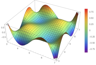
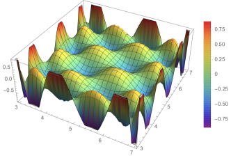
Figure 2: Graphics of the GLP W𝐦(𝐚,𝐛,𝐱)subscript𝑊𝐦𝐚𝐛𝐱W_{{\mathbf{m}}}({\mathbf{a}},{\mathbf{b}},{\mathbf{x}}) (18, 34) in 2D defined in the square [3,7]×[3,7]3737[3,7]\times[3,7] for 𝐦=(3,3)𝐦33{\mathbf{m}}=(3,3) and 𝐦=(5,7)𝐦57{\mathbf{m}}=(5,7), respectively.

This is in, say, two dimensions. The generalization to n𝑛n dimensions is straightforward.

We may generalize (33) as

n[𝐚,𝐛]n:=[a1,b1]×[a2,b2]××[an,bn],𝐚,𝐛n,formulae-sequencesuperscript𝑛superscript𝐚𝐛𝑛assignsubscript𝑎1subscript𝑏1subscript𝑎2subscript𝑏2subscript𝑎𝑛subscript𝑏𝑛𝐚𝐛superscript𝑛\mathcal{R}^{n}\equiv[{\mathbf{a}},{\mathbf{b}}]^{n}:=[a_{1},b_{1}]\times[a_{2},b_{2}]\times\cdots\times[a_{n},b_{n}]\,,\quad{\mathbf{a}}\,,\,{\mathbf{b}}\in{\mathbb{R}}^{n}\,, (37)

and the orthonormal basis (35) as

W𝐦(𝐚,𝐛,𝐱)Wm1(a1,b1,x1)Wm2(a2,b2,x2)Wmn(an,bn,xn).subscript𝑊𝐦𝐚𝐛𝐱tensor-producttensor-productsubscript𝑊subscript𝑚1subscript𝑎1subscript𝑏1subscript𝑥1subscript𝑊subscript𝑚2subscript𝑎2subscript𝑏2subscript𝑥2subscript𝑊subscript𝑚𝑛subscript𝑎𝑛subscript𝑏𝑛subscript𝑥𝑛W_{\mathbf{m}}({\bf a},{\bf b},{\bf x})\equiv W_{m_{1}}(a_{1},b_{1},x_{1})\otimes W_{m_{2}}(a_{2},b_{2},x_{2})\otimes\cdots\otimes W_{m_{n}}(a_{n},b_{n},x_{n})\,. (38)

Now, we have that 𝐦n𝐦superscript𝑛{\mathbf{m}}\in{\mathbb{N}}^{n}, 𝐚,𝐛n𝐚𝐛superscript𝑛{\mathbf{a}},\,{\mathbf{b}}\in{\mathbb{R}}^{n} and 𝐱𝐱{\mathbf{x}} belongs to [𝐚,𝐛]nsuperscript𝐚𝐛𝑛[{\mathbf{a}},{\mathbf{b}}]^{n}. Finally, the orthonormality and completeness relations can be written as, respectively,

[𝐚,𝐛]ndn𝐱W𝐦(𝐚,𝐛,𝐱)W𝐦(𝐚,𝐛,𝐱)=δ𝐦,𝐦δm1,m1δm2,m2δmn,mn,𝐦nW𝐦(𝐚,𝐛,𝐱)W𝐦(𝐚,𝐛,𝐱)=δ(𝐱,𝐱)=δ(x1x1)δ(x2x2)δ(xnxn).subscriptsuperscript𝐚𝐛𝑛superscript𝑑𝑛𝐱subscript𝑊superscript𝐦𝐚𝐛𝐱subscript𝑊𝐦𝐚𝐛𝐱subscript𝛿𝐦superscript𝐦subscript𝛿subscript𝑚1superscriptsubscript𝑚1subscript𝛿subscript𝑚2superscriptsubscript𝑚2subscript𝛿subscript𝑚𝑛superscriptsubscript𝑚𝑛missing-subexpressionmissing-subexpressionsubscript𝐦superscript𝑛subscript𝑊𝐦𝐚𝐛𝐱subscript𝑊𝐦𝐚𝐛superscript𝐱𝛿𝐱superscript𝐱𝛿subscript𝑥1superscriptsubscript𝑥1𝛿subscript𝑥2superscriptsubscript𝑥2𝛿subscript𝑥𝑛superscriptsubscript𝑥𝑛missing-subexpressionmissing-subexpression\begin{array}[]{lll}\displaystyle\int_{[{\mathbf{a}},{\mathbf{b}}]^{n}}d^{\,n}{\mathbf{x}}\,W_{\mathbf{m}^{\prime}}({{\mathbf{a}}},{{\mathbf{b}}},{{\mathbf{x}}})\,W_{\mathbf{m}}({{\mathbf{a}}},{{\mathbf{b}}},{{\mathbf{x}}})\,=\,\delta_{\mathbf{m},\mathbf{m}^{\prime}}\,\equiv\,\delta_{m_{1},m_{1}^{\prime}}\,\delta_{m_{2},m_{2}^{\prime}}\,\dots\,\delta_{m_{n},m_{n}^{\prime}}\,,\\[12.91663pt] \displaystyle\sum_{\mathbf{m}\in{\mathbb{N}}^{n}}\,W_{\mathbf{m}}({{\mathbf{a}}},{{\mathbf{b}}},{{\mathbf{x}}})\,W_{\mathbf{m}}({{\mathbf{a}}},{{\mathbf{b}}},{{\mathbf{x}}^{\prime}})\,=\,\delta({\mathbf{x}},{\mathbf{x}}^{\prime})\,=\,\delta(x_{1}-x_{1}^{\prime})\,\delta(x_{2}-x_{2}^{\prime})\,\dots\,\delta(x_{n}-x_{n}^{\prime})\,.\end{array} (39)

For every real or complex square integrable function f(𝐚,𝐛,𝐱)L2([𝐚,𝐛])𝑓𝐚𝐛𝐱superscript𝐿2𝐚𝐛f({\mathbf{a}},{\mathbf{b}},{{\mathbf{x}}})\in L^{2}([{\mathbf{a}},{\mathbf{b}}]) we have

f(𝐚,𝐛,𝐱)=𝐦=𝟎f[𝐚,𝐛]𝐦W𝐦(𝐚,𝐛,𝐱)𝑓𝐚𝐛𝐱superscriptsubscript𝐦0superscriptsubscript𝑓𝐚𝐛𝐦subscript𝑊𝐦𝐚𝐛𝐱f({{\mathbf{a}}},{{\mathbf{b}},{{\mathbf{x}}})\,=\,\sum_{{\mathbf{m}}={\mathbf{0}}}^{\infty}}\;f_{[{\mathbf{a}},{\mathbf{b}}]}^{\mathbf{m}}\;W_{\mathbf{m}}({{\mathbf{a}}},{{\mathbf{b}}},{{\mathbf{x}}}) (40)

where f[𝐚,𝐛]𝐦superscriptsubscript𝑓𝐚𝐛𝐦f_{[{\mathbf{a}},{\mathbf{b}}]}^{\mathbf{m}} are the components of f(𝐚,𝐛,𝐱)𝑓𝐚𝐛𝐱f({{\mathbf{a}}},{{\mathbf{b}}},{{\mathbf{x}}}) along W𝐦(𝐚,𝐛,𝐱)subscript𝑊𝐦𝐚𝐛𝐱W_{\mathbf{m}}({{\mathbf{a}}},{{\mathbf{b}}},{{\mathbf{x}}}) and

f[𝐚,𝐛]𝐦=[𝐚,𝐛]ndn𝐱f(𝐚,𝐛,𝐱)W𝐦(𝐚,𝐛,𝐱).superscriptsubscript𝑓𝐚𝐛𝐦subscriptsuperscript𝐚𝐛𝑛superscript𝑑𝑛𝐱𝑓𝐚𝐛𝐱subscript𝑊𝐦𝐚𝐛𝐱f_{[{\mathbf{a}},{\mathbf{b}}]}^{\mathbf{m}}\;=\;\displaystyle\int_{[{\mathbf{a}},{\mathbf{b}}]^{n}}d^{\,n}{\mathbf{x}}\;f({{\mathbf{a}},{\mathbf{b}},{\mathbf{x}}})\;W_{\mathbf{m}}({\bf a},{\bf b},{{\mathbf{x}}})\,. (41)
Refer to caption
Refer to caption
(a) K13(x1)K13(x2)tensor-productsubscript𝐾13subscript𝑥1subscript𝐾13subscript𝑥2K_{13}(x_{1})\otimes K_{13}(x_{2})                                     (b) W13(3,7,x1)W13(3,7,x2)tensor-productsubscript𝑊1337subscript𝑥1subscript𝑊1337subscript𝑥2W_{13}(3,7,x_{1})\otimes W_{13}(3,7,x_{2})
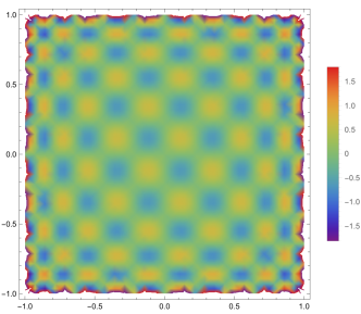
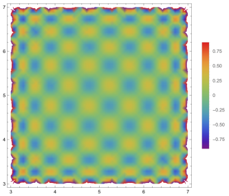
Figure 3: Density plots of: (a) the NLP in 2D K𝐦(𝐱)subscript𝐾𝐦𝐱K_{{\mathbf{m}}}({\mathbf{x}}) (18) in the square [1,1]×[1,1]1111[-1,1]\times[-1,1] with 𝐦=(13,13)𝐦1313{\mathbf{m}}=(13,13), and (b) the GLP W𝐧(𝐚,𝐛,𝐱)subscript𝑊𝐧𝐚𝐛𝐱W_{{\mathbf{n}}}({\mathbf{a}},{\mathbf{b}},{\mathbf{x}}) (18, 34) living in the square [3,7]×[3,7]3737[3,7]\times[3,7].
Refer to caption
Refer to caption
(a) W13(2,7,x1)W12(2,5,x2)tensor-productsubscript𝑊1327subscript𝑥1subscript𝑊1225subscript𝑥2W_{13}(2,7,x_{1})\otimes W_{12}(2,5,x_{2})                                     (b) W13(2,7,x1)W12(2,5,x2)tensor-productsubscript𝑊1327subscript𝑥1subscript𝑊1225subscript𝑥2W_{13}(2,7,x_{1})\otimes W_{12}(2,5,x_{2})
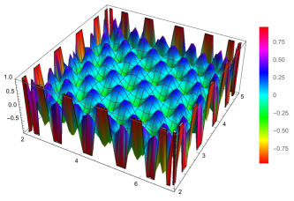
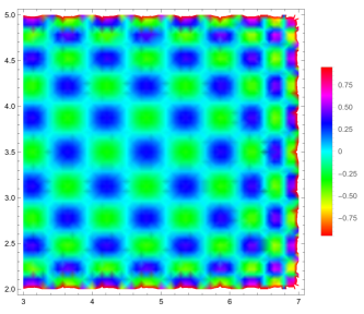
Figure 4: Graphic (a) and Density plot (b) of the GLP W𝐧(𝐚,𝐛,𝐱)subscript𝑊𝐧𝐚𝐛𝐱W_{{\mathbf{n}}}({\mathbf{a}},{\mathbf{b}},{\mathbf{x}}) (18, 34) defined in the rectangle [2,7]×[2,5]2725[2,7]\times[2,5] and 𝐦=(13,12)𝐦1312{\mathbf{m}}=(13,12).

So far, the discussion on the more general Legendre polynomials.

VI On the continuity of the generators of su(1,1)𝑠𝑢11su(1,1)

It is clear that the operators J±subscript𝐽plus-or-minusJ_{\pm} (22) and J3subscript𝐽3J_{3} (29) are unbounded on the Hilbert space L2([a,b])superscript𝐿2𝑎𝑏L^{2}([a,b]) and, hence, not defined on all vectors of the Hilbert space. Nevertheless, they have a common subdomain, such that when endowed with a locally convex topology, they become continuous under this topology. This goes through the construction of a suitable Gelfand triplet or rigged Hilbert space. Let us start with this construction for L2([a,b])superscript𝐿2𝑎𝑏L^{2}([a,b]) and then, generalize the procedure to L2([𝐚,𝐛]2)superscript𝐿2superscript𝐚𝐛2L^{2}([{\mathbf{a}},{\mathbf{b}}]^{2}), which is rather straightforward.

Thus, our goal is the construction of a triplet  Φa,bL2[(a,b])Φa,b×\Phi_{a,b}\subset L^{2}[(a,b])\subset\Phi^{\times}_{a,b},  for which we just need to determine the space Φa,bsubscriptΦ𝑎𝑏\Phi_{a,b}. Let f(x)𝑓𝑥f(x) be an arbitrary function in L2([a,b])superscript𝐿2𝑎𝑏L^{2}([a,b]), we know that this function can be spanned as

f(x)=m=1fmWm(a,b,x),withm=1|fm|2=f(x)2.formulae-sequence𝑓𝑥superscriptsubscript𝑚1superscript𝑓𝑚subscript𝑊𝑚𝑎𝑏𝑥withsuperscriptsubscript𝑚1superscriptsuperscript𝑓𝑚2superscriptnorm𝑓𝑥2f(x)=\sum_{m=1}^{\infty}f^{m}\,W_{m}(a,b,x)\,,\,\quad{\rm with}\,\quad\sum_{m=1}^{\infty}|f^{m}|^{2}=||f(x)||^{2}\,. (42)

Let us choose Φa,bsubscriptΦ𝑎𝑏\Phi_{a,b} as the space of functions f(x)L2([a,b])𝑓𝑥superscript𝐿2𝑎𝑏f(x)\in L^{2}([a,b]), as given in (42), for which

[pk(f)]2:=m=1|fm|2(m+1)2k<,k=0,1,2,.formulae-sequenceassignsuperscriptdelimited-[]subscript𝑝𝑘𝑓2superscriptsubscript𝑚1superscriptsuperscript𝑓𝑚2superscript𝑚12𝑘𝑘012[p_{k}(f)]^{2}:=\sum_{m=1}^{\infty}|f^{m}|^{2}\,(m+1)^{2k}<\infty\,,\,\qquad k=0,1,2,\dots\,. (43)

Note that, for k=0𝑘0k=0, we have the Hilbert space norm. This is a sequence of seminorms, in fact norms, that produce a locally convex topology on Φa,bsubscriptΦ𝑎𝑏\Phi_{a,b}. Since this sequence of seminorms, contains the Hilbert space norm, then, the topology on Φa,bsubscriptΦ𝑎𝑏\Phi_{a,b} is finer than the Hilbert space norm topology. Further considerations show that Φa,bsubscriptΦ𝑎𝑏\Phi_{a,b} with this topology is a complete metrizable space, and hence Frèchet simon1980 .

The series in (42) converge in the Hilbert space norm sense. Let see that for f(x)Φa,b𝑓𝑥subscriptΦ𝑎𝑏f(x)\in\Phi_{a,b}, the series (42) converge uniformly and absolutely. First of all, from the properties of the Legendre polynomials and (19), we have that

|Wm(a,b,x)|2ba.subscript𝑊𝑚𝑎𝑏𝑥2𝑏𝑎|W_{m}(a,b,x)|\leq\sqrt{\frac{2}{b-a}}\,. (44)

Then, for any f(x)Φa,b𝑓𝑥subscriptΦ𝑎𝑏f(x)\in\Phi_{a,b} with span as in (42), we have that

|m=1fmWm(a,b,x)|m=1|fm||Wm(a,b,x)|2bam=1|fm|m+1m+1.superscriptsubscript𝑚1superscript𝑓𝑚subscript𝑊𝑚𝑎𝑏𝑥superscriptsubscript𝑚1superscript𝑓𝑚subscript𝑊𝑚𝑎𝑏𝑥2𝑏𝑎superscriptsubscript𝑚1superscript𝑓𝑚𝑚1𝑚1\displaystyle\left|\sum_{m=1}^{\infty}f^{m}\,W_{m}(a,b,x)\right|\leq\sum_{m=1}^{\infty}|f^{m}|\,|W_{m}(a,b,x)|\leq\sqrt{\frac{2}{b-a}}\sum_{m=1}^{\infty}|f^{m}|\,\frac{m+1}{m+1}.
2bam=1|fm|2(m+1)2m=11(m+1)2,absent2𝑏𝑎superscriptsubscript𝑚1superscriptsuperscript𝑓𝑚2superscript𝑚12superscriptsubscript𝑚11superscript𝑚12\displaystyle\leq\sqrt{\frac{2}{b-a}}\;\sqrt{\sum_{m=1}^{\infty}|f^{m}|^{2}(m+1)^{2}}\;\sqrt{\sum_{m=1}^{\infty}\frac{1}{(m+1)^{2}}}\,, (45)

where the last inequality is just the Cauchy-Schwartz inequality. All the series converge in this last term. Then, after the Weierstrass M-Theorem, the considered series m=1fmWm(a,b,x)Φa,bsuperscriptsubscript𝑚1superscript𝑓𝑚subscript𝑊𝑚𝑎𝑏𝑥subscriptΦ𝑎𝑏\sum_{m=1}^{\infty}f^{m}\,W_{m}(a,b,x)\in\Phi_{a,b} converge absolutely and uniformly. The identity in (42) for f(x)Φa,b𝑓𝑥subscriptΦ𝑎𝑏f(x)\in\Phi_{a,b} is also pointwise.

Before proceeding with our presentation, let us give an important result: let A𝐴A be a linear operator on a locally convex space ΦΦ\Phi, for which the topology is defined by a set of seminorms (pi)iIsubscriptsubscript𝑝𝑖𝑖𝐼(p_{i})_{i\in I}. Then, A𝐴A is continuous on ΦΦ\Phi if and only if for each seminorm pisubscript𝑝𝑖p_{i}, there exist a positive number Kisubscript𝐾𝑖K_{i} and a finite set of seminorms {pi1,pi2,,pik}subscript𝑝subscript𝑖1subscript𝑝subscript𝑖2subscript𝑝subscript𝑖𝑘\{p_{i_{1}},p_{i_{2}},\dots,p_{i_{k}}\}, depending on pisubscript𝑝𝑖p_{i}, such that simon1980

pi(Af)Ki{pi1(f)+pi2(f)++pik(f)},fΦ.formulae-sequencesubscript𝑝𝑖𝐴𝑓subscript𝐾𝑖subscript𝑝subscript𝑖1𝑓subscript𝑝subscript𝑖2𝑓subscript𝑝subscript𝑖𝑘𝑓for-all𝑓Φp_{i}(A\,f)\leq K_{i}\{p_{i_{1}}(f)+p_{i_{2}}(f)+\dots+p_{i_{k}}(f)\}\,,\qquad\forall\,f\in\Phi\,. (46)

From (25), we may define J±subscript𝐽plus-or-minusJ_{\pm} on Φa,bsubscriptΦ𝑎𝑏\Phi_{a,b}. Thus, the action of J+subscript𝐽J_{+} on f(x)Φa,b𝑓𝑥subscriptΦ𝑎𝑏f(x)\in\Phi_{a,b} should be defined as

J+m=1fmWm(a,b,x):=m=1fm(m+1)Wm+1(a,b,x).assignsubscript𝐽superscriptsubscript𝑚1superscript𝑓𝑚subscript𝑊𝑚𝑎𝑏𝑥superscriptsubscript𝑚1superscript𝑓𝑚𝑚1subscript𝑊𝑚1𝑎𝑏𝑥J_{+}\sum_{m=1}^{\infty}f^{m}\,W_{m}(a,b,x):=\sum_{m=1}^{\infty}f^{m}\,(m+1)\,W_{m+1}(a,b,x)\,. (47)

We need to show that this is a good definition in the sense that the sum converges to an element of Φa,bsubscriptΦ𝑎𝑏\Phi_{a,b} and that J+subscript𝐽J_{+} is continuous on Φa,bsubscriptΦ𝑎𝑏\Phi_{a,b}. The former is just a trivial consequence of the definition of Φa,bsubscriptΦ𝑎𝑏\Phi_{a,b} (it is obviously linear). To prove the continuity, take any seminorm pksubscript𝑝𝑘p_{k}, then, for any f(x)Φa,b𝑓𝑥subscriptΦ𝑎𝑏f(x)\in\Phi_{a,b} we have

[pk(J+f)]2superscriptdelimited-[]subscript𝑝𝑘subscript𝐽𝑓2\displaystyle[p_{k}(J_{+}f)]^{2} =\displaystyle= n=1|fm|2(m+1)2(m+2)2km=1|fm|2(m+1)2(2m+2)2ksuperscriptsubscript𝑛1superscriptsuperscript𝑓𝑚2superscript𝑚12superscript𝑚22𝑘superscriptsubscript𝑚1superscriptsuperscript𝑓𝑚2superscript𝑚12superscript2𝑚22𝑘\displaystyle\sum_{n=1}^{\infty}|f^{m}|^{2}\,(m+1)^{2}\,(m+2)^{2k}\leq\sum_{m=1}^{\infty}\,|f^{m}|^{2}\,(m+1)^{2}\,(2m+2)^{2k} (48)
=\displaystyle= 22km=1|fm|2(m+1)2(k+1)=22k[pk+1f]2,k=0,1,2,,formulae-sequencesuperscript22𝑘superscriptsubscript𝑚1superscriptsuperscript𝑓𝑚2superscript𝑚12𝑘1superscript22𝑘superscriptdelimited-[]subscript𝑝𝑘1𝑓2𝑘012\displaystyle 2^{2k}\sum_{m=1}^{\infty}\,|f^{m}|^{2}\,(m+1)^{2(k+1)}=2^{2k}\,[p_{k+1}f]^{2}\,,\quad k=0,1,2,\dots\,,

which, after (46), shows the continuity of J+subscript𝐽J_{+} on Φa,bsubscriptΦ𝑎𝑏\Phi_{a,b}.

The definition of Jsubscript𝐽J_{-} should be given by

Jm=1fmWm(a,b,x):=m=2fmmWm1(a,b,x).assignsubscript𝐽superscriptsubscript𝑚1superscript𝑓𝑚subscript𝑊𝑚𝑎𝑏𝑥superscriptsubscript𝑚2superscript𝑓𝑚𝑚subscript𝑊𝑚1𝑎𝑏𝑥J_{-}\sum_{m=1}^{\infty}f^{m}\,W_{m}(a,b,x):=\sum_{m=2}^{\infty}f^{m}\,m\,W_{m-1}(a,b,x)\,. (49)

The operator Jsubscript𝐽J_{-} is obviously linear and well defined on Φa,bsubscriptΦ𝑎𝑏\Phi_{a,b}. Furthermore, for all f(x)Φa,b𝑓𝑥subscriptΦ𝑎𝑏f(x)\in\Phi_{a,b}

[pk(Jf)]2=m=2|fm|2m2(m1+1)2km=1|fm|2(m+1)2(k+1)=[pk+1f]2,k=0,1,2,.formulae-sequencesuperscriptdelimited-[]subscript𝑝𝑘subscript𝐽𝑓2superscriptsubscript𝑚2superscriptsuperscript𝑓𝑚2superscript𝑚2superscript𝑚112𝑘superscriptsubscript𝑚1superscriptsuperscript𝑓𝑚2superscript𝑚12𝑘1superscriptdelimited-[]subscript𝑝𝑘1𝑓2𝑘012[p_{k}(J_{-}f)]^{2}=\sum_{m=2}^{\infty}|f^{m}|^{2}\,m^{2}\,(m-1+1)^{2k}\leq\sum_{m=1}^{\infty}|f^{m}|^{2}\,(m+1)^{2(k+1)}=[p_{k+1}f]^{2}\,,\quad k=0,1,2,\dots\,. (50)

This shows the continuity of Jsubscript𝐽J_{-} on Φa,bsubscriptΦ𝑎𝑏\Phi_{a,b}. Analogously, we define J3subscript𝐽3J_{3} on Φa,bsubscriptΦ𝑎𝑏\Phi_{a,b} as

J3m=1fmWm(a,b,x)=m=1fm(m+12)Wm(a,b,x).subscript𝐽3superscriptsubscript𝑚1superscript𝑓𝑚subscript𝑊𝑚𝑎𝑏𝑥superscriptsubscript𝑚1superscript𝑓𝑚𝑚12subscript𝑊𝑚𝑎𝑏𝑥J_{3}\sum_{m=1}^{\infty}f^{m}\,W_{m}(a,b,x)=\sum_{m=1}^{\infty}f^{m}\,\left(m+\frac{1}{2}\right)\,W_{m}(a,b,x)\,. (51)

By repeating the same argument, we show that J3subscript𝐽3J_{3} is well defined and continuous on Φa,bsubscriptΦ𝑎𝑏\Phi_{a,b}. Note that all the three operators, as well as their products and linear combinations may be extended by continuity to the dual Φa,b×subscriptsuperscriptΦ𝑎𝑏\Phi^{\times}_{a,b}, provided that this dual be endowed with any topology compatible with the dual pair, usually the weak or the strong topologies HOR .

These results may be extended to the general situation studied in Section 5. In the simplest case of dimension equal to two, an arbitrary function f(𝐱)L2([𝐚,𝐛]2)𝑓𝐱superscript𝐿2superscript𝐚𝐛2f(\mathbf{x})\in L^{2}([\mathbf{a},\mathbf{b}]^{2}) can be written as (42)

f(𝐱)f(x1,x2)=𝐦=𝟎f[𝐚,𝐛]𝐦W𝐦(𝐚,𝐛,𝐱)=m1,m2=0f[𝐚,𝐛]m1,m2Wm1(a1,b1,x1)Wm2(a2,b2,x2).𝑓𝐱𝑓subscript𝑥1subscript𝑥2superscriptsubscript𝐦0superscriptsubscript𝑓𝐚𝐛𝐦subscript𝑊𝐦𝐚𝐛𝐱superscriptsubscriptsubscript𝑚1subscript𝑚20subscriptsuperscript𝑓subscript𝑚1subscript𝑚2𝐚𝐛subscript𝑊subscript𝑚1subscript𝑎1subscript𝑏1subscript𝑥1subscript𝑊subscript𝑚2subscript𝑎2subscript𝑏2subscript𝑥2f(\mathbf{x})\equiv f(x_{1},x_{2})=\sum_{{\mathbf{m}}={\mathbf{0}}}^{\infty}\;f_{[{\mathbf{a}},{\mathbf{b}}]}^{\mathbf{m}}\;W_{\mathbf{m}}({{\mathbf{a}}},{{\mathbf{b}}},{{\mathbf{x}}})=\sum_{m_{1},m_{2}=0}^{\infty}f^{m_{1},m_{2}}_{[{\mathbf{a}},{\mathbf{b}}]}\,W_{m_{1}}(a_{1},b_{1},x_{1})\,W_{m_{2}}(a_{2},b_{2},x_{2})\,. (52)

The space Φ𝐚,𝐛subscriptΦ𝐚𝐛\Phi_{\mathbf{a},\mathbf{b}} is defined as the space of functions f(x1,x2)L2([𝐚,𝐛])𝑓subscript𝑥1subscript𝑥2superscript𝐿2𝐚𝐛f(x_{1},x_{2})\in L^{2}([\mathbf{a},\mathbf{b}]) such that (see (40))

[pk1,k2f]2:=m1,m2=0|f[𝐚,𝐛]m1,m2|2(m1+1)2k1(m2+1)2k2<,k1,k2=0,1,2,.formulae-sequenceassignsuperscriptdelimited-[]subscript𝑝subscript𝑘1subscript𝑘2𝑓2superscriptsubscriptsubscript𝑚1subscript𝑚20superscriptsubscriptsuperscript𝑓subscript𝑚1subscript𝑚2𝐚𝐛2superscriptsubscript𝑚112subscript𝑘1superscriptsubscript𝑚212subscript𝑘2subscript𝑘1subscript𝑘2012[p_{k_{1},k_{2}}f]^{2}:=\sum_{{m_{1}},{m_{2}}=0}^{\infty}\big{|}f^{m_{1},m_{2}}_{[{\mathbf{a}},{\mathbf{b}}]}\big{|}^{2}\,(m_{1}+1)^{2k_{1}}\,(m_{2}+1)^{2k_{2}}<\infty\,,\quad k_{1},k_{2}=0,1,2,\dots\,. (53)

All the tensor products of the operators J±subscript𝐽plus-or-minusJ_{\pm} and J3subscript𝐽3J_{3} (also their linear combinations and products) act linearly and are continuous on Φ𝐚,𝐛subscriptΦ𝐚𝐛\Phi_{\mathbf{a},\mathbf{b}}. Proofs are exactly as above for dimension one. The extension of all these ideas to n dimensions is straightforward.

VII Concluding remarks

In this paper we present a generalization of the Legendre polynomials to any finite interval [a,b]𝑎𝑏[a,b] of the real line. These new functions, W(m,a,b,x)𝑊𝑚𝑎𝑏𝑥W(m,a,b,x), constitute an orthonormal and countable basis for the square integrable functions defined in this interval. We use these functions to construct bases in ‘n𝑛n-rectangular’ domains n=[a1,b1]×[a2,b2]××[an,bn]nsuperscript𝑛subscript𝑎1subscript𝑏1subscript𝑎2subscript𝑏2subscript𝑎𝑛subscript𝑏𝑛superscript𝑛\mathcal{R}^{n}=[a_{1},b_{1}]\times[a_{2},b_{2}]\times\dots\times[a_{n},b_{n}]\subset{\mathbb{R}}^{n} as W(m1,a1,b1,x1)W(m2,a2,b2,x2)W(mn,an,bn,xn)tensor-producttensor-product𝑊subscript𝑚1subscript𝑎1subscript𝑏1subscript𝑥1𝑊subscript𝑚2subscript𝑎2subscript𝑏2subscript𝑥2𝑊subscript𝑚𝑛subscript𝑎𝑛subscript𝑏𝑛subscript𝑥𝑛W(m_{1},a_{1},b_{1},x_{1})\otimes W(m_{2},a_{2},b_{2},x_{2})\otimes\dots\otimes W(m_{n},a_{n},b_{n},x_{n}).

A practical application of this construction is the reconstruction of images in an ‘analogical’ procedure in 2D or 3D either in black and white or in color. To this end, we span some function in terms of series of W𝑊W-functions and just keep a finite number of terms. Note that from the enormous contents of information of an image, we -the humans- can just use a minimal part. The problem is to give a criteria on how to obtain the relevant part of the information. Digital images cannot produce this section, essentially because they produce a restriction to averages on all neighbourhoods of constant dimension of the image. The analogical procedure presented in this paper illustrates a smooth realization of the image where the average is not homogeneous, but instead shared according to the values of W𝑊W around an arbitrary center with arbitrary magnification. This idea can be used in general. For instance, it may have applications in medicine as an implementation of Ref. levenson . In this paper, the authors describe how images of breast cancer can be analysed with great efficiency by trained groups of pigeons (Columba livia). In addition, this shows that informations on the pathology are already contained into the image and the problem that remains is to isolate the image from the background.

Acknowledgements

The paper has been parcially supported by MCIN of Spain with funding from the European Union NextGenerationEU (PRTRC17.I1) and the PID2020-113406GB-IO project by MCIN. E. Celeghini would like to thank the University of Valladolid for its hospitality.

References

  • (1) S, Qi, Y. Zhang, C. Wang, J. Zhou and X. Cao, “A Survey of Orthogonal Moments for Image Representation: Theory, Implementation, and Evaluation”, ACM Computing Surveys 55 1-35 (2023).
  • (2) W. A. Jassim, P. Raveendran and R. Mukundan, “New orthogonal polynomials for speech signal and image processing”, Signal Processing, IET 6 713-72 (2012).
  • (3) K. W. See, K. S. Loke, P. A. Lee and K. F. Loe, “Image reconstruction using various discrete orthogonal polynomials in comparison with DCT”, Applied Mathematics and Computation 193 346-359 (2007).
  • (4) J. Zhou, H. Shu, H. Zhu, C. Toumoulin and L., Luo, “Image analysis by discrete orthogonal Hahn moments”, in M. Kamel, A. Campilho (eds), Image Analysis and Recognition. ICIAR 2005. Lecture Notes in Computer Science, vol 3656, pp. 524-531 (Springer, Berlin, Heidelberg 2005); https://doi.org/10.1007/11559573-65 .
  • (5) O. Hunt and R. Mukunda, “Image coding using orthogonal basis functions” Rep. Comput. Graphics Image Processing Res. Group (2004); https://api.semanticscholar.org/CorpusID:16690597.
  • (6) P. T. Yap, R. Paramesran and S. H. Ong, “Image analysis by Krawtchouk moments”, IEEE Trans. Image Proc. 12 1367-1377 (2003).
  • (7) R. Mukundan, S. H. Ong and P. A. Lee, “Image analysis by Tchebichef moments”. IEEE Trans. Image Proc. 1357-1364 (2001).
  • (8) M. R. Teague, “Image analysis via the general theory of moments”, J. Opt. Soc. Am. 70 920-930 (1980).
  • (9) M. K. Hu, “Visual pattern recognition by moment invariants” IRE Trans. Inf. Theory 8 179-187 (1962).
  • (10) R. Mukundan and K. R. Ramakrishnan, “Fast computation of Legendre and Zernike moments”, Pattern Recognit. 28 1433-42 (1995).
  • (11) Chong C W, Raveendran P and Mukundan R 2004 Translation and scale invariants of Legendre moments Pattern Recognit. 37 119-129
  • (12) P. T. Yap and R. Paramesran, “An efficient method for the computation of Legendre moments” IEEE Trans. on Pattern Analysis and Machine Intelligence 27 1996-2002 (2005).
  • (13) B. Xiao, G. Wang and W. Li, “Radial shifted Legendre moments for image analysis and invariant image recognition”, Image Vis. Comput. 32 994-1006 (2014).
  • (14) T. Yang, J. Ma, Y. Miao, X. Liu, X. Wang and Q. Meng, “PLCOM: Privacy-preserving outsourcing computation of Legendre circularly orthogonal moment over encrypted image data”, Inf. Sci. 505 198-214 (2019).
  • (15) M. Hosny, M. M. Darwish and T. Aboelenen, “New fractional-order Legendre-Fourier moments for pattern recognition applications”, Pattern Recognit. 103 107324 (2020).
  • (16) G. Szegö, Orthogonal Polynomials (Am. Math. Soc.: Providence, R.I., USA, 2003).
  • (17) E. Celeghini and M. A. del Olmo, “Coherent orthogonal polynomials” Ann. of Phys. 335 78-85 (2013). https://doi.org/10.1016/j.aop.2013.04.017
  • (18) A-M Legendre, “ Recherches sur l’attraction des sphéroïdes homogènes”, Mémoires de Mathématiques et de Physique, présentés à l’Académie Royale des Sciences par divers savans, et lus dans ses Assemblées X 411-435 (1785).
  • (19) J. Wagemans, F. J. H. Elder, M. Kubovy, S. E. Palmer, M. A. Peterson, M. Singh and R. von der Heydt, “Century of Gestalt Psychology in Visual Perception:I. Perceptual Grouping and Figure-Ground Organization”, Psychological Bulletin 138 1172-1217 (2012).
  • (20) J. Wagemans, J. Feldman, S. Gepshtein, R. Kimchi, J. R. Pomerantz, P. A. van der Helm and C. van Leeuwen, “A century of Gestalt psychology in visual perception: II. Conceptual and theoretical foundations” Psychological Bulletin 138 1218-1252 (2012).
  • (21) F. Zernike, “Beugungstheorie des schneidenver-fahrens und seiner verbesserten form, der phasenkontrastmethode”, Physica 1 689-704 (1934).
  • (22) E. Celeghini, “Theory of Images and Quantum Mechanics, a common paradigm”, J. Phys,: Conf. Ser. 880 012055 (2017).
  • (23) E. Celeghini, M. Gadella and M. A. Olmo, “Zernike functions, rigged Hilbert spaces, and potential applications”, J. Math. Phys. 60, 083508 (2019).
  • (24) E. Celeghini, M. Gadella and M. A. Olmo, “Symmetry Groups, Quantum Mechanics and Generalized Hermite Functions”, Mathematics 10 1448 ( 2022).
  • (25) I. M. Gelfand and N. Y. Vilenkin, Generalized Functions: Applications to Harmonic Analysis, vol. 4 ( Academic, New York, 1964).
  • (26) J. E. Roberts, “Rigged Hilbert spaces in quantum mechanics”, Commun. Math. Phys. 3 98-119 (1966).
  • (27) J. P. Antoine, “Dirac Formalism and Symmetry Problems in Quantum Mechanics. I. General Dirac Formalism”, J. Math. Phys. 10 , 53-69 (1969).
  • (28) O. Melsheimer, “Rigged Hilbert space formalism as an extended mathematical formalism for quantum systems. I. General theory”, J. Math. Phys. 15 902-916 (1974).
  • (29) M. Gadella and F. Gómez, “Dirac formulation of quantum mechanics: Recent and new results”, Rep. Math. Phys. 59 127-143 (2007).
  • (30) A. Bohm, The Rigged Hilbert Space and Quantum Mechanics, Lecture Notes in Physics 78 (Springer, Berlin, 1978).
  • (31) E. Celeghini, M. Gadella and M. A. Olmo, “Applications of rigged Hilbert spaces in quantum mechanics and signal processing”, J. Math. Phys. 57 072105 (2016).
  • (32) S. Cambanis, “Bases in L2subscript𝐿2L_{2} spaces with applications to stochastic processes with orthogonal increments”, 1971 Proc. Amer. Math. Soc. 29 284-290 (1971).
  • (33) M. Gadella and F. Gómez, “On the Mathematical Basis of the Dirac Formulation of Quantum Mechanics”, Int. J. Theor. Phys. 42, 2225-2254 (2003).
  • (34) M. Gadella and F. Gómez, “A measure-theoretical approach to the nuclear and inductive spectral theorems”, Bull. Sci. Math. 129 567-590 (2005).
  • (35) E. Celeghini, M. Gadella and M. A. Olmo, “Groups, Jacobi functions and rigged Hilbert spaces”, J. Math. Phys. 61 033508 (2020).
  • (36) F. W. J. Olver, D. W. Lozie, R. F. Boisiert and C. W. Clark (Eds.), NIST Handbook of Mathematical Functions (Cambridge Univ. Press: Cambridge Ma, 2010)
  • (37) M. Reed and B. Simon, Methods of Modern Mathematical Physics: Functional Analysis I (San Diego: Academic Press, 1980)
  • (38) J. Horvath, Topological vector spaces and Distributions, (Addison-Wesley, New York, 1966).
  • (39) R. M. Levenson, E. A. Krupinski, V. M. Navarro and E. A. Wasserman, “Pigeons (Columba livia) as Trainable Observers of Pathology and Radiology Breast Cancer Images”, Images. PLoS ONE 10(11): e0141357 (2015).