MURP: Multi-Agent Ultra-Wideband Relative Pose Estimation
with Constrained Communications in 3D Environments

Abstract

Inter-agent relative localization is critical for many multi-robot systems operating in the absence of external positioning infrastructure or prior environmental knowledge. We propose a novel inter-agent relative 3D pose estimation system where each participating agent is equipped with several ultra-wideband (UWB) ranging tags. Prior work typically supplements noisy UWB range measurements with additional continuously transmitted data, such as odometry, leading to potential scaling issues with increased team size and/or decreased communication network capability. By equipping each agent with multiple UWB antennas, our approach addresses these concerns by using only locally collected UWB range measurements, a priori state constraints, and detections of when said constraints are violated. Leveraging our learned mean ranging bias correction, we gain a 19% positional error improvement giving us experimental mean absolute position and heading errors of 0.24m and 9.5^∘ respectively. When compared to other state-of-the-art approaches, our work demonstrates improved performance over similar systems, while remaining competitive with methods that have significantly higher communication costs. Additionally, we make our datasets available.

I Introduction

Multi-robot systems can be used to improve the efficiency and robustness of large-scale tasks such as search & rescue [1], warehouse automation [2], and planetary exploration [3]. To operate and parallelize effectively, these systems typically need to know where the agent (and its peers) are located in a common reference frame. In practice this is often achieved by localizing within an a priori map or using an external measurement system like GPS or motion capture (mocap) [4, 5]. If these technologies are unavailable or infeasible, common approaches utilize both relative localization [6] and multi-agent SLAM [7] techniques.

Figure 1: Diagram of proposed system. Here three agents fly at different altitudes while performing real-time 3D relative pose estimation. Each agent is equipped with six ultra-wideband (UWB) antennas, each capable of performing pairwise relative ranging between all other agents’ individual antennas. By using trilateration, an improved sensor model, and a priori state constraints about altitude/roll/pitch, agents can perform instantaneous estimation entirely with locally collected UWB measurements (i.e., without the need to continuously transmit other measurements, such as odometry). Additionally, each agent locally monitors its a priori constraints via downward facing LiDAR and IMU, and thus only needs to transmit one-off messages with the swarm if these assumptions change or are violated.

Within the last decade, ultra-wideband (UWB) has matured into a reliable, inexpensive, and commercially available RF solution for data transmission, relative ranging, and localization – UWB now comes as standard issue in many popular smartphone devices [8]. For robotics, UWB has several properties of note: precision of approximately 10cm, ranges up to 100m, resilience to multipath, operates in non-line of sight (NLOS) conditions, low power consumption, and 100Mbit/s communication speeds [9]. Recent devices even extend the recommended and operational ranges to 300m and 500m respectively [10]. Nevertheless, UWB measurements are not immune from ranging errors or noise (see Section III-A), the modeling and correction of which is an active area of research [11, 12, 13, 14].

A common approach in UWB relative localization work fuses noisy UWB ranging measurements with additional continuously transmitted data, such as odometry [15] and visual inter-agent tracks [16, 17]. While these approaches achieve low absolute position error (APE) and absolute heading error (AHE), there are two prevalent shortcomings: (1) They often use a simplistic UWB measurement noise model (i.e., zero mean Gaussian), which then requires the use of supplementary measurements to compensate. (2) Reliance on these supplementary measurements (often not locally collected, e.g., odometry), mandates their continuous transmission between agents, potentially impacting scalability to increased swarm size or decreased communication throughput.

Our previous work [18] used UWB to demonstrate an instantaneous multi-tag approach to relative 2D pose estimation that achieved superior mean position accuracy and competitive performance on other metrics to Cao et al. [15] (the most comparable state-of-the-art work) using only local UWB measurements. These results were achieved by a trilateration nonlinear least squares (NLLS) optimization problem that, leveraging an improved UWB sensor model, accounted for various sources of measurement error.

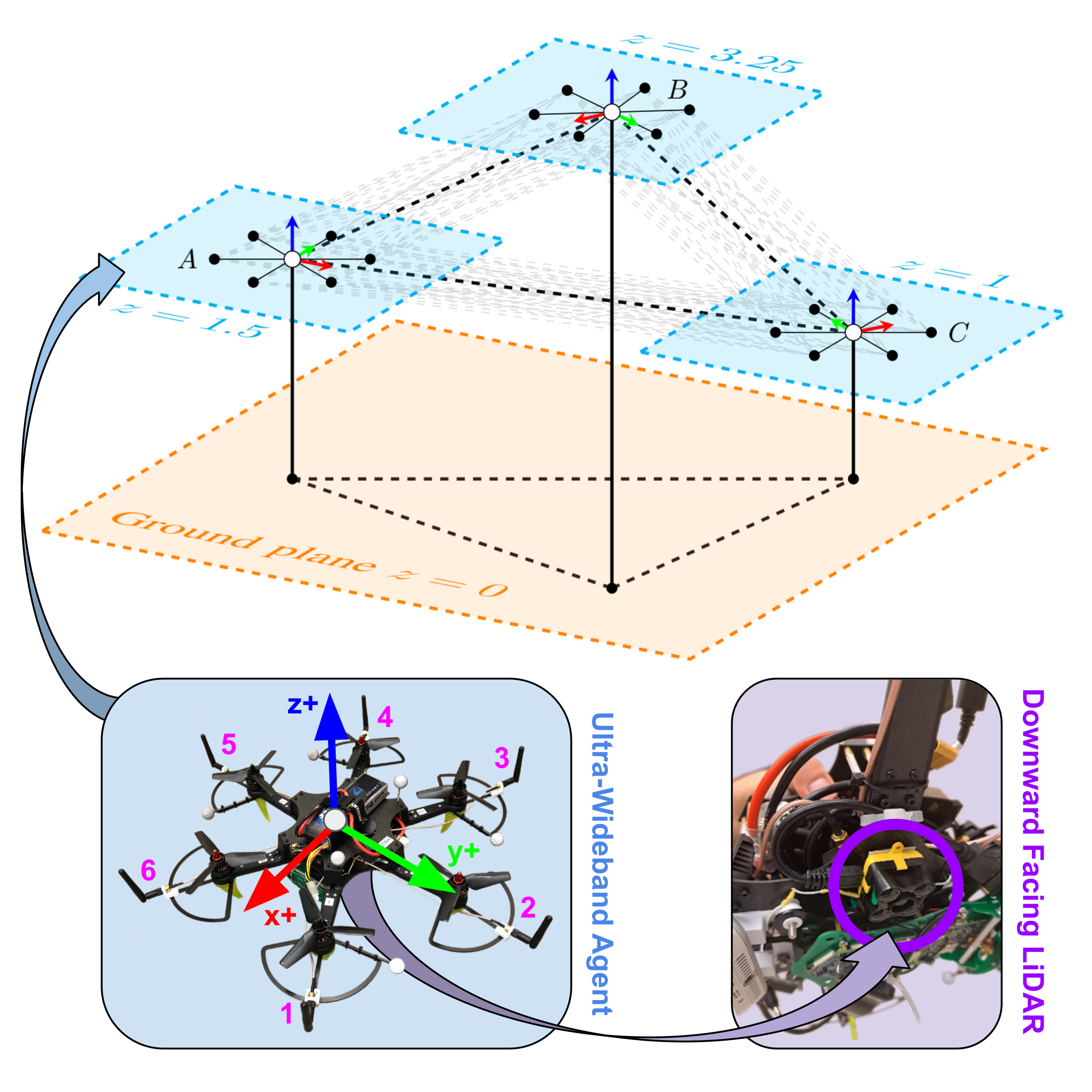
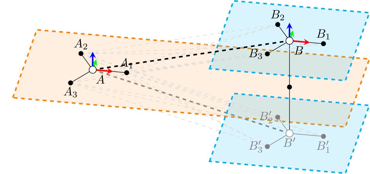
This letter extends our prior 2D work [18] to an instantaneous multi-tag relative pose estimate in 3D environments (Figure 1). Similar to our previous work, a key objective is to develop an approach that minimizes the communication load (i.e., we are willing to trade off absolute accuracy for reduced communication overhead). In 3D environments, each agent’s altitude/roll/pitch are locally measurable with respect to the world frame (e.g., via altimeter or downward facing LiDAR and IMU). By constraining each agent to an altitude/roll/pitch envelope, this information only needs to be transmitted once a priori. These assumptions can then be locally monitored by each agent, with one-off communication occurring only to alert the swarm a constraint has been violated (i.e., one-off messages only communicate a new constraint envelope if it has changed, or let the swarm know to ignore the agent until further notice). By leveraging and monitoring these state constraints, we simplify the 6-DoF optimization (i.e., 3D position and orientation) to a 3-DoF optimization (i.e., $x$, $y$, yaw with known $z$, roll, pitch) that, with fewer free variables, more reliably produces 3D localization solutions. Thus our approach provides a 3D relative pose using only locally collected UWB range measurements, a priori state constraints, and detections of constraint violations.

This paper’s contributions are: (1) An in-depth analysis and modeling of the observed noise characteristics of 3D UWB ranging measurements (Section III). (2) A 3D solution for UWB-based relative localization, formulated as a robust nonlinear least squares optimization with minimal communication footprint and locally monitored assumptions. We utilize a learned measurement bias correction as a function of relative elevation that accounts for observed noise properties, improving our mean absolute position error by 19% (Section V). (3) Experimental results that demonstrate the merits of our proposed solution, a mean APE and AHE of 0.24m and 9.5^∘ respectively without continuously transmitting measurements (Section VI). (4) Our datasets, over 200 hours of pairwise UWB range measurements with ground truth, for use by the larger robotics community.

(a)

(b)

(c)

(d)

Figure 2: Plots demonstrating the UWB noise and geometry characteristics outlined in Section III. (a) A histogram of our entire dataset’s UWB measurements binned by range error. Demonstrates a non-zero mean and a long tail (i.e., violates the zero mean Gaussian assumption used by many works). (b) The same data plotted as error with respect to relative elevation. Here, we see the measurement error’s mean and variance significantly change with relative elevation. The dotted blue line represents a learned 6-degree polynomial fit of measurement bias. (c) Simple example demonstrating dilution of precision (DOP) in a 2D ranging scenario. Here, the red and green points have known baselines of 3m and 6m respectively. Each red/green point independently measures the distance to the blue point with a consistent uncertainty of $\pm 1$m. To estimate the position of the blue point, the red and green points each intersect their uncertain measurements, respectively creating red and green feasibility regions. Despite having the same uncertainty on all range measurements, the green points (i.e., the larger baseline) produce a smaller uncertainty region than the red points. (d) This diagram demonstrates how three (or more) ranging antennas within a single plane produce a pair of ambiguous solutions (i.e., if all antennas are in the base’s plane $z=0$, while the target’s $x$ and $y$ coordinates are fully observable, the target’s altitude has an ambiguity between $\pm z$).

II Related Works

TABLE I: Comparison of relevant related works to highlight the capability gap this letter fills. Color emphasizes how a work fits in with our goals. Specifically, green indicates our needs are met, yellow indicates our needs are partially met, and red indicates our needs are not met.

2D / 3D	Related Work	# UWB  Per Agent	UWB Noise Model	Data Exchanged
2D	Guo et al.     (2020) [19]	Single	Bounded Error Assumption	UWB + Velocity
	Cao et al.     (2021) [15]	Many (4)	NLLS	UWB + Odometry
	Zheng et al.     (2022) [20]	Many (2 or 4)	ZM Gaussian + NLOS Rejection	UWB + VIO
	Zhang et al.     (2023) [21]	Many (2 or 4)	ZM Gaussian + Outlier Rejection	UWB + Point Clouds + Odom + Keyframes
	[Our Prev. Work]     (2022) [18]	Many (4)	NLLS + Data Informed Sensor Model	UWB
3D	Xu et al.     (2020) [16]	Single	ZM Gaussian	UWB + VIO + Visual Tracks
	Qi et al.       (2020) [22]	Single	ZM Gaussian	UWB + IMU + GPS Heading
	Xianjia et al.     (2021) [23]	Many (2 or 4)	NLLS	UWB
	Xu et al.     (2022) [17]	Single	ZM Gaussian + Occlusion Rejection	UWB + VIO + Visual Tracks
	Xun et al.     (2023) [24]	Single	ZM Gaussian	UWB + IMU + IR Visual Tracks
	[This Work]     (2023)	Many (4 or 6)	NLLS + Data Informed Sensor Model	UWB + One-Off Assumption Violations

UWB technology can be leveraged by mobile robotics in several orthogonal ways. This work uses UWB for infrastructure-free inter-agent relative measurements – thus, works involving GPS position, static UWB anchors, UWB radar, or measurements done by direct waveform analysis are out of scope of this letter [25, 26, 27] (see survey paper [28] or our previous work [18] for a broader review of UWB in robotics). Table I highlights the unique capability gap this work fills with respect to the recent related literature. While all works in Table I use UWB for inter-agent ranging, it is challenging to compare numerical results given the vastly different operating assumptions and priorities – specifically access to additional sensors (e.g., cameras, LiDAR, etc.), the size of agents with respect to their environment (see Section III-B), and overall communication model (e.g., unlimited vs constrained communication) all significantly change performance and scalability. To contextualize this work, we discuss [21] and [17] since they are the most complete and comprehensive 2D and 3D UWB systems respectively, [24] since it has a unique compact hardware solution, and [23] since it is the most directly comparable to this work.

Zhang et al. [21] presents a centralized 2D range-aided cooperative localization and consistent reconstruction system, merging a tightly coupled visual odometry and multi-tag ranging front-end with a pose graph optimization (PGO) back-end. This work differs from ours by being 2D and relying on continuous transmission of point cloud, odometry, and keyframe information. Omni-swarm [17] is a decentralized 3D swarm estimation system. This work differs from ours by relying primarily on visual tracks of neighboring agents from each agent’s omnidirectional camera – omitting UWB measurements only degrades estimation by approximately 0.01m. Additionally, each agent has only a single UWB tag and requires continuously sharing measurements between all pairs of agents, scaling poorly with larger swarms. CREPES [24] presents a custom compact hardware module, which tightly couples an IMU, UWB, IR LEDs, and IR fish-eye camera. The measurements are fused into 6-DoF relative pose via a centralized error-state Kalman filter (ESKF) and PGO, while also having the ability to provide an instantaneous estimate from a single frame of sensor measurements. This work differs from ours by relying heavily on visual tracks over UWB (similar to [17]). Additionally, the system relies on continuously transmitted measurements. Thus the state of the art approaches in [21, 17, 24] achieve APE and AHE on the order of 0.10 m and $1^{\circ}$, respectively, but they require additional sensors (e.g., LiDAR, fish-eye cameras, etc.) that must continuously transmit measurements, making them scale poorly to scenarios with larger swarm sizes or reduced communication throughput.

Xianjia et al. [23] is the most similar to our work (i.e., 3D environment, multiple UWB tags per agent, and using only UWB measurements). When their agents have similar antenna baselines to our work, they achieve a mean $xy$-positional error of approximately 0.40m, 0.65m, and 0.85m for simulated 8m$\times$8m flights at various fixed altitudes. Furthermore, for real flights the mean $xy$-positional error becomes approximately 1m with a variable altitude and a (beneficial) larger baseline. By comparison, although our experimental environment differs, we achieve a mean APE and AHE of 0.24m and $9.5^{\circ}$ respectively with real experiments operating in a 10m$\times$10m mocap space. Ref. [23] differs from our approach in two important ways: (1) the authors model UWB ranging error as a zero mean Gaussian with a 0.10m standard deviation, which does not reflect real data (see Section III-A); and (2) we define an explicit communication protocol that allows us to address several capability gaps without continuously transmitting measurements. Specifically, by constraining altitude/roll/pitch and improving our UWB noise model, we can better address UWB noise (see Section III-A) and an observability ambiguity (see Section III-B and Figure 2(d)). See Section III-C for more details.

III Extensions to 3D Environments

The following subsections motivate our hardware and algorithmic choices for operating in 3D (Section III-C). We first characterize the UWB ranging error of the Nooploop LinkTrack P-B [10] from a set of initial experiments (Section III-A), and then provide the observability and error properties of trilateration-based localization (Section III-B).

III-A Characterizing UWB Noise

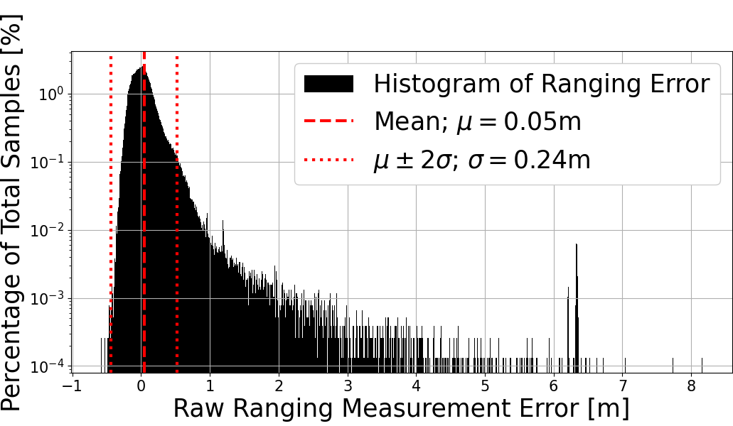
Long Tail Distributions: Contrary to common noise assumptions in Table I, individual UWB ranging errors appear neither zero mean nor Gaussian. Instead, error distributions have long positive tails (see Figure 2(a)). A trend towards positive bias can be attributed to the many ways positive ranging error can be introduced to a UWB measurement (e.g., change of propagation medium, multipath). Furthermore, installing SMA cables between the RF device and antenna adds a consistent positive bias to all measurements.

Sensitivity to Obstruction: Antenna obstruction (i.e., NLOS conditions) introduces positive bias and increased variance to collected ranging measurements (see Figure 4(b)). While the UWB protocol is resilient to multipath and NLOS, UWB ranging is not completely absolved of these concerns. Furthermore, auxiliary metrics, like RSSI, do not appear to meaningfully indicate an obstructed measurement. Ref. [20, 21, 18, 17] address this by rejecting suspect measurements, whether detected via statistical tests, robust loss functions, or hardcoded rejection criteria.

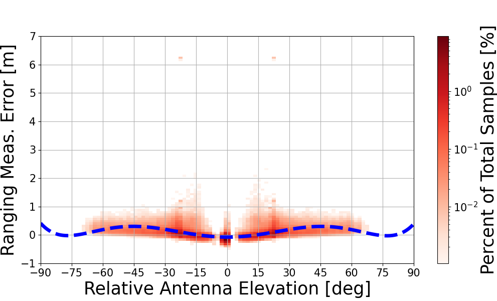
Dependence on Relative Pose: Measurement noise is dependent on relative pose between antennas. The interplay of antenna attenuation patterns is a core concern of RF designers, but gets understandably overlooked by many end users. The LinkTrack P series comes equipped with a standard dipole antenna which we would expect to produce the behavior observed in Figure 2(b) when aligned upright [10] – specifically, approximately uniform performance within an $xy$-plane (i.e., varying azimuth) and degraded performance outside the ground plane $z=0$ (i.e., non-zero elevation). We note that both the mean bias and variance change with elevation. A relationship to elevation is noted in [17], although it is attributed to NLOS conditions similar to Figure 4(b), but [17] chooses to address this by simply omitting range measurements with more than $37^{\circ}$ relative elevation (feasible only because of their reliance on other measurements).

III-B Geometry of Ranging-based Pose Estimation

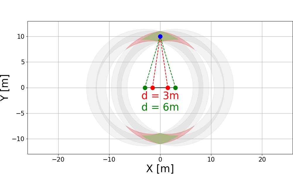
Observability of Position: In 3D trilateration, a minimum of 4 non-coplanar antennas are required to uniquely determine a target’s position [29]. That being said, 3 or more planar antennas produce only a pair of solutions that are a reflection across the antenna plane (see Figure 2(d)). This ambiguity can be resolved with a simple $z$ measurement (i.e., altitude).

Observability of Pose: Common in camera-robot registration, Horn’s Method is a closed-form solution for finding the pose between two Cartesian coordinate systems from a set of corresponding point pairs [30]. Specifically, given exactly 3 planar points in two frames with known correspondences, Horn’s Method fully specifies the 3D translation and orientation. Thus, by using trilateration to measure 3 points in a known configuration on our target, we can recover full pose.

Dilution of Precision: Most commonly associated with GPS, dilution of precision (DOP) is a trilateration sensitivity analysis for quantifying how 1D ranging errors propagate to 2D/3D point estimation error [31]. Specifically, given trilateration’s nonlinear nature, even identically noisy 1D range measurements can produce wildly different 2D/3D positional uncertainties – this is entirely determined by the given base station geometry (see Figure 2(c)). In general we note that increasing the distance between base stations (i.e., the “baseline”), or being closer to the base stations, reduces trilateration’s sensitivity. See [20, 21] for a detailed discussion of DOP as it pertains to 2D UWB localization. This also accounts for the improved accuracy seen by [23] for configurations with larger baselines. Thus, the accuracy of trilateration systems with vastly different baselines or operating ranges can be misleading.

III-C System Design

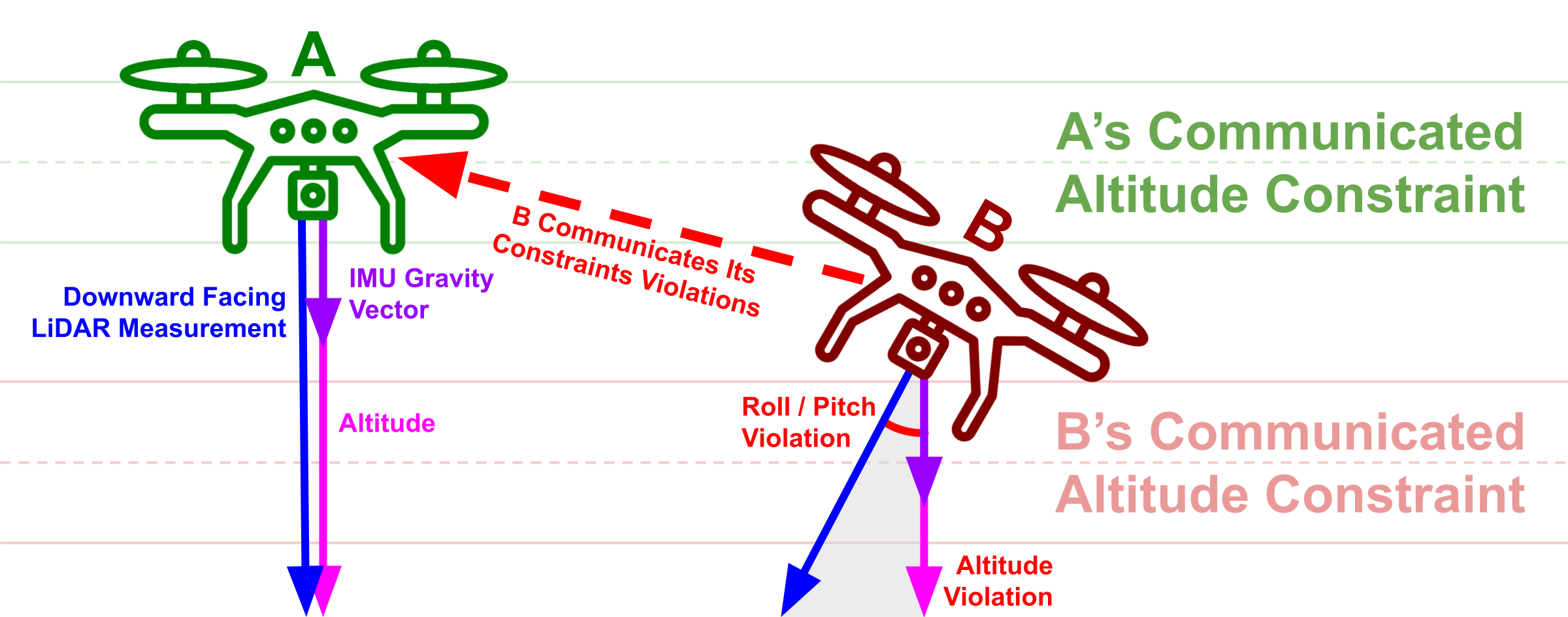
Based on the noise characteristics (Section III-A) and underlying geometry (Section III-B), we propose the system design shown in Figure 1 for our multirotor drones. Specifically, each agent is equipped with 6 ranging antennas each attached at the end of their propeller arms (i.e., 0.31m from the center) to maximize baseline distances and create better DOP geometry. Since there are 6 coplanar antennas, this is an over-constrained problem that still has a $\pm z$ ambiguity across the $z=0$ plane. Although an additional nonplanar antenna can be to each agent, it is challenging to get a significant $z$-baseline without creating poor flight conditions (i.e., prohibitively heavy or awkward center of mass). Instead, we note that altitude/roll/pitch can be measured within the flat-ground world frame locally via altimeter or downward facing LiDAR and onboard IMU. In many drone applications, it is common for multirotors to maintain roll/pitch near $0^{\circ}$ and a constant altitude. Thus we can specify a minimalist communication protocol that shares these intended constraints a priori and then monitors them locally to ensure they are maintained. One-off communication occurs only when a constraint is locally detected to have been violated/changed (see Figure 3(b)). Additionally, having a constant $z$ constraint helps mitigate the increased variance associated with relative elevation (see Figure 2(b)).

(a)

(b)

Figure 3: (a) Annotated diagram of three UGV agents used in Section VI-B. UGV agents are designed with the same baseline as the UAV in Figure 1, making them comparable surrogates to the UAV and its experiments in Section VI-A. (b) Diagram demonstrating agent $B$ locally detecting violations in its a priori constraints, triggering a one-off communication.

IV Preliminaries

IV-A Pose Parameterization

Given a set of 3D reference frames $\mathcal{F}$, consider any pair of frames $A\in\mathcal{F}$ and $B\in\mathcal{F}$. Let $\mathbf{T}^{A}_{B}\in SE(3)$ be the relative pose between frames $A$ and $B$ (i.e., transforms a point from $B$’s frame into $A$’s frame). We note $\mathbf{T}^{A}_{B}$ is a 6-DoF value that can be equivalently parameterized as the 2-tuple $\langle\mathbf{R}^{A}_{B},\mathbf{t}^{A}_{B}\rangle$ or 6-tuple $\langle x^{A}_{B},y^{A}_{B},z^{A}_{B},\alpha^{A}_{B},\beta^{A}_{B},\gamma^{A}_{B}\rangle$, where:

• $\mathbf{R}^{A}_{B}\in SO(3)$ is the relative rotation between $A$ and $B$ parameterized by the 3-tuple of Euler angles $\langle\alpha,\beta,\gamma\rangle$, where $\alpha^{A}_{B}\in[-180^{\circ},180^{\circ}]$ is relative roll, $\beta^{A}_{B}\in[-90^{\circ},90^{\circ}]$ is relative pitch, and $\gamma^{A}_{B}\in[-180^{\circ},180^{\circ}]$ is relative yaw. The use of Euler angles over quaternions is motivated by the direct roll/pitch constraints to be introduced Equation 7. We define $\mathbf{R}(\alpha,\beta,\gamma)$ as the $\mathbb{R}^{3\times 3}$ rotation matrix with respect to $\mathbf{R}_{x}(\alpha)$, $\mathbf{R}_{y}(\beta)$, $\mathbf{R}_{z}(\gamma)$, the $\mathbb{R}^{3\times 3}$ rotation matrices about the $x$, $y$, $z$ axes respectively. Thus $\mathbf{R}^{A}_{B}$ can be equivalently represented as a $\mathbb{R}^{3\times 3}$ rotation matrix in the following ways:

  $$\mathbf{R}^{A}_{B}\triangleq\mathbf{R}(\alpha^{A}_{B},\beta^{A}_{B},\gamma^{A}_{B})\triangleq\mathbf{R}_{z}(\gamma^{A}_{B})\mathbf{R}_{y}(\beta^{A}_{B})\mathbf{R}_{x}(\alpha^{A}_{B})$$

• $\mathbf{t}^{A}_{B}\in\mathbb{R}^{3}$ is a relative translation vector between $A$ and $B$ parameterized by the 3-tuple $\langle x^{A}_{B},y^{A}_{B},z^{A}_{B}\rangle$. Thus, $\mathbf{t}^{A}_{B}$ can be equivalently represent in the following ways:

  $$\mathbf{t}^{A}_{B}\triangleq\mathbf{t}(x^{A}_{B},y^{A}_{B},z^{A}_{B})\triangleq\begin{bmatrix}x^{A}_{B}&y^{A}_{B}&z^{A}_{B}\end{bmatrix}^{\top}$$

IV-B Rigid Body Transformations

For any frame $F\in\mathcal{F}$, let $\mathbf{p}^{F}\in\mathbb{R}^{3}$ be a point in frame $F$. Given $\mathbf{T}^{A}_{B}$ (i.e., the relative pose between frames $A$ and $B$), points $\mathbf{p}^{A}$ and $\mathbf{p}^{B}$ (i.e., the same point but in $A$’s or $B$’s frame respectively) are related by:

$$\mathbf{p}^{A}=\mathbf{R}^{A}_{B}\mathbf{p}^{B}+\mathbf{t}^{A}_{B}$$

which can equivalently and succinctly be written in homogeneous coordinate notation [32] as:

$$\breve{\mathbf{p}}^{A}=\mathbf{T}^{A}_{B}\breve{\mathbf{p}}^{B}$$

where $\mathbf{T}^{A}_{B}\in\mathbb{R}^{4\times 4}$ and $\breve{\mathbf{p}}^{F}\in\mathbb{R}^{4}$ are defined as:

$$\mathbf{T}^{A}_{B}\triangleq\begin{bmatrix}\mathbf{R}^{A}_{B}&\mathbf{t}^{A}_{B}\\ \mathbf{0}^{\top}&1\end{bmatrix}\qquad\qquad\breve{\mathbf{p}}^{F}\triangleq\begin{bmatrix}\mathbf{p}^{F}\\ 1\end{bmatrix}$$

Thus $\mathbf{T}^{A}_{B}$ is equivalently represented in the following ways:

$$\mathbf{T}^{A}_{B} \triangleq\mathbf{T}(x^{A}_{B},y^{A}_{B},z^{A}_{B},\alpha^{A}_{B},\beta^{A}_{B},\gamma^{A}_{B})$$

$$\triangleq\begin{bmatrix}\mathbf{R}^{A}_{B}&\mathbf{t}^{A}_{B}\\ \mathbf{0}^{\top}&1\end{bmatrix}\triangleq\begin{bmatrix}\mathbf{R}(\alpha^{A}_{B},\beta^{A}_{B},\gamma^{A}_{B})&\mathbf{t}(x^{A}_{B},y^{A}_{B},z^{A}_{B})\\ \mathbf{0}^{\top}&1\end{bmatrix}$$

V Technical Approach

Algorithm 1 Procedure for robot $A\in\mathcal{R}$, a member of robot swarm $\mathcal{R}$, to generate instantaneous relative poses w.r.t. all other agents in swarm $B\in(\mathcal{R}\setminus\{A\})$

1:$\mathcal{R}$, $A\in\mathcal{R}$, $\{\mathcal{I}_{R}~{}\forall~{}R\in\mathcal{R}\}$, $\ell$

2:$\{~{}\mathbf{T}^{A}_{B}~{}\forall~{}B\in(\mathcal{R}\setminus\{A\})\text{ s.t. }\neg\texttt{invalid}(B)~{}\}$

3:function LocalProcedure

4:     $\tilde{\bm{\kappa}}_{A}\leftarrow$ local measurements of $A$ w.r.t. $W$

5:     if $\neg(|\hat{\bm{\kappa}}_{A}-\tilde{\bm{\kappa}}_{A}|\leq\check{\bm{\kappa}}_{A})$ then

6:         $\texttt{transmit}(A)$

7:     end if

8:     $\mathcal{T}\leftarrow\{\}$

9:     for $B\in(\mathcal{R}\setminus\{A\})\text{ s.t. }\neg\texttt{invalid}(B)$ do

10:         $\tilde{\mathbf{d}}^{A}_{B}\leftarrow$ local measurements of $B$ w.r.t. $A$

11:         $\langle\hat{z}^{A}_{B},\hat{\alpha}^{A}_{B},\hat{\beta}^{A}_{B}\rangle\leftarrow\hat{\bm{\kappa}}^{W}_{B}-\hat{\bm{\kappa}}^{W}_{A}$

12:         $\langle x^{A}_{B},y^{A}_{B},\gamma^{A}_{B}\rangle\leftarrow$ optimize Eq. 9

13:         $\mathbf{T}^{A}_{B}\leftarrow\mathbf{T}(x^{A}_{B},y^{A}_{B},\hat{z}^{A}_{B},\hat{\alpha}^{A}_{B},\hat{\beta}^{A}_{B},\gamma^{A}_{B})$

14:         $\mathcal{T}\leftarrow\mathcal{T}\cup\{\mathbf{T}^{A}_{B}\}$

15:     end for

16:     return $\mathcal{T}$

17:end function

V-A Local Robot Definitions

Let there be some 3D world frame $W$ defined with respect to the level ground and gravity vector (i.e., $z=0$ is the “floor” and gravity faces down). Consider $\mathcal{R}$, a set of $N_{\mathcal{R}}$ robots operating in $W$. Each robot $R\in\mathcal{R}$, has $N_{R}$ relative ranging antennas rigidly affixed to $R$’s body, where $R_{k}$ denotes $R$’s $k$th antenna. Additionally, for each $R$ let there be an a priori and static 3-tuple of known information $\mathcal{I}_{R}=\langle\hat{\bm{\kappa}}_{R},\check{\bm{\kappa}}_{R},\mathcal{P}_{R}\rangle$, where:

• $\hat{\bm{\kappa}}_{R}=\begin{bmatrix}\hat{z}^{W}_{R}&\hat{\alpha}^{W}_{R}&\hat{\beta}^{W}_{R}\end{bmatrix}^{\top}$ is a vector of constant global state constraints on $R$ with respect to world frame $W$. In other words, $\hat{z}^{W}_{R}$ is the commanded altitude, while $\hat{\alpha}^{W}_{R}$ and $\hat{\beta}^{W}_{R}$ are commanded relative roll and pitch.

• $\check{\bm{\kappa}}_{R}=\begin{bmatrix}\check{z}^{W}_{R}&\check{\alpha}^{W}_{R}&\check{\beta}^{W}_{R}\end{bmatrix}^{\top}$ is a vector of constant absolute (i.e., $\pm$) tolerances on global constraints $\hat{\bm{\kappa}}_{R}$.

• $\mathcal{P}_{R}=\{\mathbf{T}^{R}_{R_{1}},\mathbf{T}^{R}_{R_{2}},\dots,\mathbf{T}^{R}_{R_{N_{R}}}\}$ is an ordered set of $N_{R}$ constant relative poses from $R$’s body frame to $R$’s $k$th antenna’s frame. Additionally, from the information in $\mathbf{T}^{R}_{R_{k}}$, we can succinctly denote the point coordinate of $R$’s $k$th antenna in $R$’s frame as $\mathbf{p}^{R}_{k}$.

Since $W$ is defined with respect to a level ground and gravity vector, the parameters $\langle z^{W}_{R},\alpha^{W}_{R},\beta^{W}_{R}\rangle$ – unlike $\langle x^{W}_{R},y^{W}_{R},\gamma^{W}_{R}\rangle$ – are instantaneously observable and directly measurable from $R$ (e.g., via altimeter or downward facing LiDAR and onboard IMU). Thus, the directly measured values $\tilde{\bm{\kappa}}_{R}=\begin{bmatrix}\tilde{z}^{W}_{R}&\tilde{\alpha}^{W}_{R}&\tilde{\beta}^{W}_{R}\end{bmatrix}^{\top}$ can be continuously monitored by $R$ locally (i.e., without relying on swarm communication). After an initial one-off transmission of $\mathcal{I}_{R}$ to all agents $\mathcal{R}$, agent $R$ only needs to transmit again in the event of (1) wanting to change its commanded altitude/roll/pitch $\hat{\bm{\kappa}}_{R}$, or (2) it locally observes a violation of its previously communicated constraints, specifically:

$$\underbrace{|\hat{\bm{\kappa}}_{R}-\tilde{\bm{\kappa}}_{R}|}_{\text{element-wise abs deviation}}\leq\underbrace{\check{\bm{\kappa}}_{R}}_{\text{constraint tolerance}}$$ (1)

where $|\cdot|$ and $\leq$ are performed element-wise. In other words, all agents $\mathcal{R}$ can treat $\hat{\bm{\kappa}}_{R}$ as known states during estimation, unless $R$ communicates otherwise.

V-B Inter-Agent Robot Definitions

Consider any arbitrary pair of robots $A\in\mathcal{R}$ and $B\in\mathcal{R}$. With a slight abuse of notation, let $A$ and $B$ also denote the robots respective reference frames, making $\mathbf{T}^{A}_{B}$ denote the relative pose between robots $A$ and $B$. From our known information tuples $\mathcal{I}_{A}$ and $\mathcal{I}_{B}$ we know each agent has ${N_{A}}$ and ${N_{B}}$ antennas at relative poses $\mathcal{P}_{A}$ and $\mathcal{P}_{B}$ respectively. This in turn allows us to define our observation model as just a function of $\mathbf{T}^{A}_{B}$. In other words, the distance between $A$’s $i$th antenna and $B$’s $j$th antenna is defined as:

$$d^{A_{i}}_{B_{j}}(\mathbf{T}^{A}_{B})\triangleq||\mathbf{T}^{A}_{B}\breve{\mathbf{p}}^{B}_{j}-\breve{\mathbf{p}}^{A}_{i}||_{2}$$ (2)

where $d^{A_{i}}_{B_{j}}(\mathbf{T}^{A}_{B})\in\mathbb{R}_{\geq 0}$, as distances are non-negative, and $||\cdot||_{2}$ denotes the $L_{2}$ norm. Similarly, let $\tilde{d}^{A_{i}}_{B_{j}}$ be the current (i.e., most recent) noisy measurement between $A$’s $i$th antenna and $B$’s $j$th antenna as measured locally by $A$. For convenience, $\tilde{\mathbf{d}}^{A}_{B}\in\mathbb{R}^{{N_{A}}{N_{B}}}$ denotes the stacked vector of all current pairwise $\tilde{d}^{A_{i}}_{B_{j}}$ measurements.

V-C Noise Model Definition

Let $\mathbf{T}^{A_{i}}_{B_{j}}$ denote the relative pose between $A$’s $i$th antenna and $B$’s $j$th antenna. Given a known $\mathcal{P}_{A}$ and $\mathcal{P}_{B}$, and an arbitrary $\mathbf{T}^{A}_{B}$, we have:

$$\mathbf{T}^{A_{i}}_{B_{j}}=(\mathbf{T}^{A}_{A_{i}})^{-1}\mathbf{T}^{A}_{B}\mathbf{T}^{B}_{B_{j}}=\mathbf{T}^{A_{i}}_{A}\mathbf{T}^{A}_{B}\mathbf{T}^{B}_{B_{j}}$$ (3)

so that $\mathbf{T}^{A_{i}}_{B_{j}}$ is a function of $\mathbf{T}^{A}_{B}$ given known $\mathcal{P}_{A}$ and $\mathcal{P}_{B}$. Let $\bar{d}(\mathbf{T}^{A_{i}}_{B_{j}})\in\mathbb{R}$ be some provided (e.g., learned) sensor mean bias model as a function of $\mathbf{T}^{A_{i}}_{B_{j}}$ (i.e., antenna measurement bias is modeled as some function of the relative position and/or orientation between a pair of ranging antennas). We can then equivalently define:

$$\bar{d}^{A_{i}}_{B_{j}}(\mathbf{T}^{A}_{B})\triangleq\bar{d}(\mathbf{T}^{A_{i}}_{A}\mathbf{T}^{A}_{B}\mathbf{T}^{B}_{B_{j}})$$ (4)

where $\bar{d}^{A_{i}}_{B_{j}}(\mathbf{T}^{A}_{B})\in\mathbb{R}$ is a state-dependent mean bias estimate for measurement $\tilde{d}^{A_{i}}_{B_{j}}$.

V-D Optimization Definition

Using our current measurements $\tilde{d}^{A_{i}}_{B_{j}}$, measurement bias correction function $\bar{d}^{A_{i}}_{B_{j}}(\mathbf{T}^{A}_{B})$, and observation model $d^{A_{i}}_{B_{j}}(\mathbf{T}^{A}_{B})$, we can formulate the error residual function with respect to antenna pair ${A_{i}}$ and ${B_{j}}$ as:

$$e^{A_{i}}_{B_{j}}(\mathbf{T}^{A}_{B})\triangleq\underbrace{\Big{(}\tilde{d}^{A_{i}}_{B_{j}}-\bar{d}^{A_{i}}_{B_{j}}(\mathbf{T}^{A}_{B})\Big{)}}_{\text{bias adjusted measurement}}-\underbrace{d^{A_{i}}_{B_{j}}(\mathbf{T}^{A}_{B})}_{\text{expected measurement}}$$ (5)

Using our error residual function $e^{A_{i}}_{B_{j}}(\mathbf{T}^{A}_{B})$, and some loss function $\ell$, we can calculate an instantaneous estimate of $\mathbf{T}^{A}_{B}$ by minimizing the sum of loss of all error residuals for all inter-agent antenna pairs with respect to $\mathbf{T}^{A}_{B}$. That is:

$$\min_{\mathbf{T}^{A}_{B}\in SE(3)}\sum_{i=1}^{{N_{A}}}\sum_{j=1}^{{N_{B}}}\ell\Big{(}e^{A_{i}}_{B_{j}}(\mathbf{T}^{A}_{B})\Big{)}$$ (6)

Recall that $\mathbf{T}^{A}_{B}$ is a 6-DoF variable parameterized by $\langle x^{A}_{B},y^{A}_{B},z^{A}_{B},\alpha^{A}_{B},\beta^{A}_{B},\gamma^{A}_{B}\rangle$. From known information tuples $\mathcal{I}_{A}$ and $\mathcal{I}_{B}$, we have $\hat{\bm{\kappa}}_{A}$ and $\hat{\bm{\kappa}}_{B}$, which provide us with constraints $\langle\hat{z}^{W}_{A},\hat{\alpha}^{W}_{A},\hat{\beta}^{W}_{A}\rangle$ and $\langle\hat{z}^{W}_{B},\hat{\alpha}^{W}_{B},\hat{\beta}^{W}_{B}\rangle$. Furthermore, since these constraints are with respect to a common world frame $W$, see that: $\hat{z}^{A}_{B}=\hat{z}^{W}_{B}-\hat{z}^{W}_{A}$, $\hat{\alpha}^{A}_{B}=\hat{\alpha}^{W}_{B}-\hat{\alpha}^{W}_{A}$, and $\hat{\beta}^{A}_{B}=\hat{\beta}^{W}_{B}-\hat{\beta}^{W}_{A}$. Thus, given $\hat{\bm{\kappa}}_{A}$ and $\hat{\bm{\kappa}}_{B}$, we have the following constrained optimization:

$$\begin{split}\min_{\mathbf{T}^{A}_{B}\in SE(3)}\quad&\sum_{i=1}^{{N_{A}}}\sum_{j=1}^{{N_{B}}}\ell\Big{(}e^{A_{i}}_{B_{j}}(\mathbf{T}^{A}_{B})\Big{)}\\ \text{s.t.}\quad&z^{A}_{B}=\hat{z}^{A}_{B}=\hat{z}^{W}_{B}-\hat{z}^{W}_{A}\\ &\alpha^{A}_{B}=\hat{\alpha}^{A}_{B}=\hat{\alpha}^{W}_{B}-\hat{\alpha}^{W}_{A}\\ &\beta^{A}_{B}=\hat{\beta}^{A}_{B}=\hat{\beta}^{W}_{B}-\hat{\beta}^{W}_{A}\end{split}$$ (7)

which can then be simplified to an equivalent 3-DoF unconstrained optimization problem:

which can be rewritten as $f$ to clearly see the dependencies:

$$\min_{\begin{subarray}{c}x^{A}_{B},y^{A}_{B}\in\mathbb{R}\\ \gamma^{A}_{B}\in[-180^{\circ},180^{\circ}]\end{subarray}}f(x^{A}_{B},y^{A}_{B},\gamma^{A}_{B}~{}|~{}\tilde{\mathbf{d}}^{A}_{B},\mathcal{I}_{A},\mathcal{I}_{B},\ell)$$ (9)

That is, given our current ranging measurements $\tilde{\mathbf{d}}^{A}_{B}$, our known information tuples $\mathcal{I}_{A}$ and $\mathcal{I}_{B}$, and some loss function $\ell$, our 3D pose can be found as 3-DoF minimization of our free variables $\langle x^{A}_{B},y^{A}_{B},\gamma^{A}_{B}\rangle$.

Using Equation 9, Algorithm 1 outlines a procedure independently followed by each agent $A$ in a swarm $\mathcal{R}$ to individually estimate $\mathbf{T}^{A}_{B}$ between itself and all other agents $B\in(\mathcal{R}\setminus\{A\})$. Observe that one-off communication (i.e., transmit) only occurs on Line 4, when an agent locally detects it has violated its a priori constraints – this is then used by other agents on Line 7 (i.e., invalid) to skip calculating $\mathbf{T}^{A}_{B}$ for agents with violated constraints.

TABLE II: Evaluation of positional error in meters with different $z$-constraints. In practice, the second row (i.e., a priori constraints) will be used, but the small difference between z_comm, z_meas, and z_true shows these constraints are not a major source of error. See Section VI-A.

Abs Position Error [m]		Scenarios (Section VI-A)
		Trial 1			Trial 2			Trial 3
color	alt constraint	Mean	Max	Std	Mean	Max	Std	Mean	Max	Std
	z_free	1.17	2.83	1.06	1.04	1.53	0.24	0.45	0.94	0.19
$\blacksquare$	z_comm	0.26	0.45	0.09	0.28	0.87	0.14	0.25	0.64	0.13
$\blacksquare$	z_meas	0.26	0.44	0.09	0.27	0.87	0.14	0.24	0.66	0.14
$\blacksquare$	z_true	0.25	0.44	0.10	0.26	0.87	0.15	0.22	0.64	0.14

(a) Shows Table II’s Trial 2 alongside the commanded, measured, and ground truth altitude, where the colors correspond with Table II. While the TeraRanger Evo does not perfectly track ground truth, it stays within the expected commanded tolerance providing a reasonable local measurement of altitude.

(b) Top plot shows calibrated ranging error (i.e., mean bias subtracted) w.r.t. relative yaw for the 1m above and level flights (i.e., Trial 4 and 5 respectively). Observe the error of 1m above flight remains consistent, while the level flight has anomalous error peaks corresponding to specific relative yaws. The lower left and right diagrams show the relative pose of the agents at the two most prominent peaks, where the path between antennas $A_{1}$ and $B_{5}$ is eclipsed by antennas $B_{3}$ and $B_{1}$ respectively. While this NLOS effect is consistent with our previous 2D work [18], we note the more complex 3D relationship resolves the occlusion with varying elevation.

Figure 4: Plots from the UAV flight experiments.

TABLE III: Evaluation of positional error in meters between algorithms. The final row represents the proposed approach. See Section VI-B.

Abs Position Error [m]				Scenarios (Section VI-B)
				Trial 1			Trial 2			Trial 3			Trial 4			Trial 5
color	el_bias	z_fixed	Huber	Mean	Max	Std	Mean	Max	Std	Mean	Max	Std	Mean	Max	Std	Mean	Max	Std
$\blacksquare$				2.21	4.40	1.17	0.89	4.50	0.88	2.37	4.82	1.13	2.26	4.58	1.12	2.77	4.32	0.59
	✓			2.55	4.95	0.64	0.89	4.46	0.97	1.32	3.94	0.95	1.33	3.97	0.97	1.55	3.71	0.90
		✓		0.45	2.87	0.38	0.42	1.50	0.28	0.57	2.97	0.52	0.45	2.40	0.36	0.40	1.16	0.23
	✓	✓		0.34	2.86	0.43	0.34	1.49	0.32	0.53	2.96	0.55	0.38	2.41	0.39	0.30	1.16	0.28
$\blacksquare$			✓	1.14	3.29	1.12	2.15	3.29	1.03	1.24	3.60	1.01	2.30	3.57	1.02	1.30	3.24	1.16
$\blacksquare$	✓		✓	0.44	1.64	0.30	0.95	2.58	0.90	0.85	3.10	0.75	0.85	2.69	0.82	1.44	2.88	0.90
$\blacksquare$		✓	✓	0.29	0.91	0.14	0.27	1.02	0.14	0.32	1.03	0.20	0.28	0.78	0.14	0.29	0.71	0.13
$\blacksquare$	✓	✓	✓	0.22	0.90	0.17	0.21	0.98	0.16	0.30	0.97	0.21	0.23	0.75	0.15	0.22	0.63	0.14

TABLE IV: Evaluation of yaw error in meters between algorithms. The final row represents the proposed approach. See Section VI-B.

Abs Heading Error [deg]				Scenarios (Section VI-B)
				Trial 1			Trial 2			Trial 3			Trial 4			Trial 5
color	el_bias	z_fixed	Huber	Mean	Max	Std	Mean	Max	Std	Mean	Max	Std	Mean	Max	Std	Mean	Max	Std
$\blacksquare$				13.4	133.0	18.8	10.0	139.9	12.2	15.0	146.0	19.3	15.5	129.6	19.2	13.1	162.2	14.0
	✓			13.4	134.8	18.8	10.0	139.9	12.1	15.1	146.0	19.5	15.6	132.9	19.4	13.3	162.1	14.0
		✓		13.5	132.8	18.8	10.1	139.9	12.1	15.0	146.5	19.3	15.5	131.9	19.3	13.2	152.4	13.5
	✓	✓		13.8	133.0	18.7	10.4	139.0	12.2	15.0	146.2	19.3	16.8	170.1	23.1	14.0	166.7	14.4
$\blacksquare$			✓	8.0	47.5	5.5	7.7	177.7	12.8	8.5	57.5	6.1	10.1	111.4	10.7	10.4	47.5	7.6
$\blacksquare$	✓		✓	7.8	47.7	5.7	7.8	177.3	12.8	8.5	57.3	6.1	10.3	111.2	11.0	10.4	46.5	7.6
$\blacksquare$		✓	✓	7.6	42.4	5.1	7.6	172.6	12.5	8.3	58.4	6.1	10.4	122.0	11.2	10.6	48.5	7.6
$\blacksquare$	✓	✓	✓	8.6	46.7	5.8	8.4	172.8	12.8	8.7	59.8	6.5	10.7	111.8	11.2	11.0	42.3	7.7

(a) Proposed approach (red) generally outperforms other approaches with respect to absolute position error – only a few select points being the exception.

(b) Proposed approach (red) generally equivalent to other approaches with respect to absolute heading error, but is outperformed at a few select points.

Figure 5: Error vs Time plots for Trial 2 in Table IV and IV respectively. The line color corresponds with the algorithm’s color column in the associated tables. Each colored dashed line represent that algorithm’s overall mean in that trial.

VI Experimental Results

We present two sets of experiments: UAV (Section VI-A) and UGV (Section VI-B). We first verify the 3D noise properties, flight hardware, and show altitude/roll/pitch constraints can be sufficiently locally monitored on a UAV. Once this is verified, we confidently attach surrogate UAVs at different altitudes to UGVs – this allows us to collect data more efficiently to evaluate our approach.

VI-A UAV Experiments

Hardware: Two agents, $A$ and $B$, were used. $A$, a surrogate quadcopter, was a stationary Turtlebot2 UGV with 4 UWB sensors evenly distributed in the $xy$-plane 0.37m from the center (Same robot used in prior work [18]). As pictured in Figure 1, $B$ is a custom hexrotor equipped with 6 UWB sensors evenly distributed in the $xy$-plane 0.31m from the center. Additionally, $B$ is equipped with a downward facing TeraRanger Evo 15m LiDAR for altitude measurements [33].

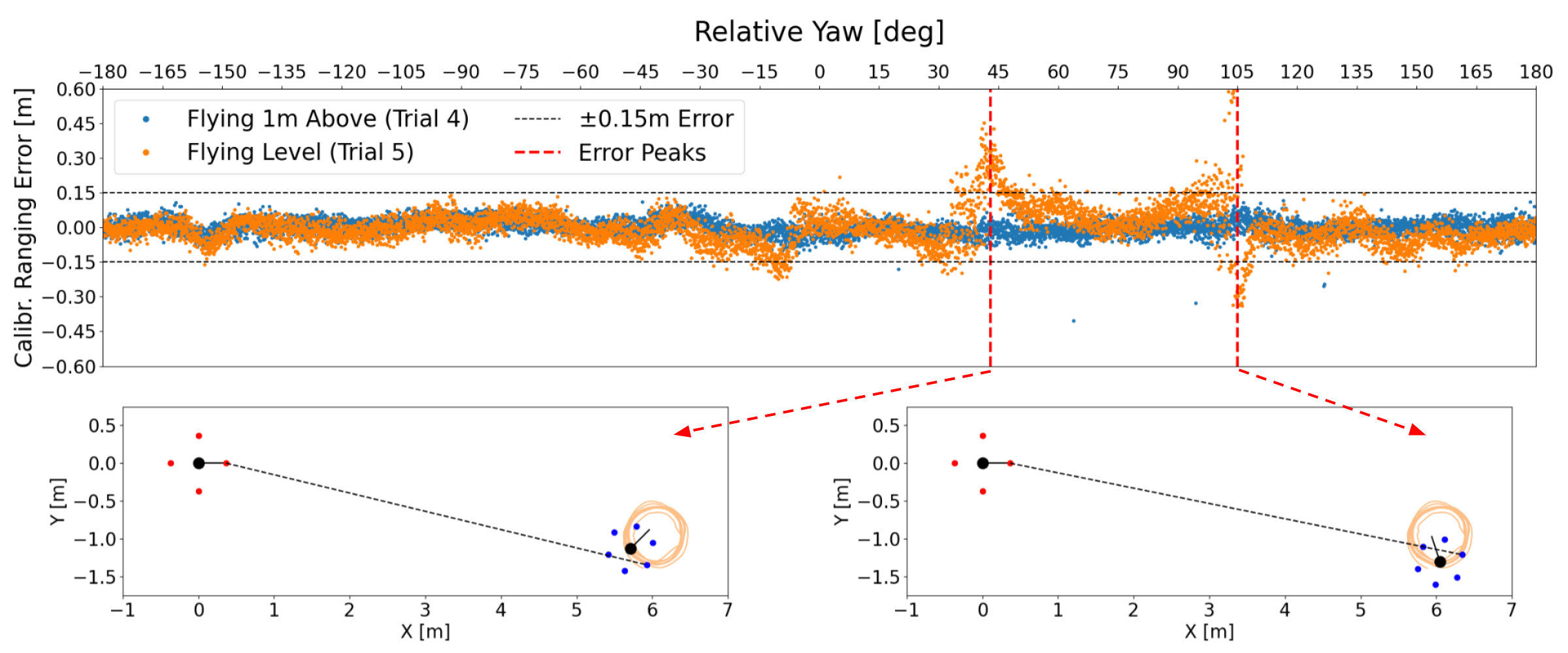
Trials: Five experimental trials were conducted in a large 10m$\times$10m mocap space. For all trials, $A$ was placed on a table for additional height and kept stationary, while $B$ flew around. In the first three trials, $B$ took off and flew simple line patterns at different altitudes (see Table II and Figure 4(a)). For the latter two trials, $B$ flew tight circles in the center of the room – first 1m above and then level with $A$ (see Figure 4(b)). Each trial had a max speed of 1m/s and lasted approximately 3-5min (i.e., the length of a battery charge).

Discussion of Results: Results are shown in Figure 4 and Table II. The main takeaways are: (1) Verified UWB measurements were not corrupted by EMI of nearby propeller motors. (2) Confirmed the robot’s body and other antennas cause significant NLOS measurement noise and bias when eclipsing a measurement path. In our previous 2D work [18], obstruction was only a function of relative azimuth and yaw and was addressed by a custom weighting function. In 3D, the addition of $\langle z,\alpha,\beta\rangle$ makes this relationship overall more complex – that being said, when agents are not in the same $z$-plane and remain level, these NLOS effects go away (see Figure 4(b)). Future work will explore modeling this entire relationship as a neural net directly within $\bar{d}^{A_{i}}_{B_{j}}(\mathbf{T}^{A}_{B})$, but for this work a robust Huber loss function (see Section VI-B) is sufficient for agents when $\Delta z\neq 0$. (3) Confirmed the onboard downward facing LiDAR and IMU can locally monitor altitude/roll/pitch accurately with only small variation from the mocap ground truth. Figure 4(a) shows Table II’s Trial 2, convincing us the TeraRanger Evo provides a reasonable local measurement of altitude. Table II shows the results of the proposed algorithm when $z$ is free (z_free), or fixed to the commanded (z_comm), LiDAR measured (z_meas), or true (z_true) value. The small APE difference between the latter three shows variation within our a priori tolerances is not a major source of error, and we can detect if we leave said bounds. This validates our minimal communication model. (4) Together, these takeaways give us confidence that surrogate UAVs attached at different altitudes to UGVs are sufficient to fairly evaluate our approach in Section VI-B.

VI-B UGV Experiments

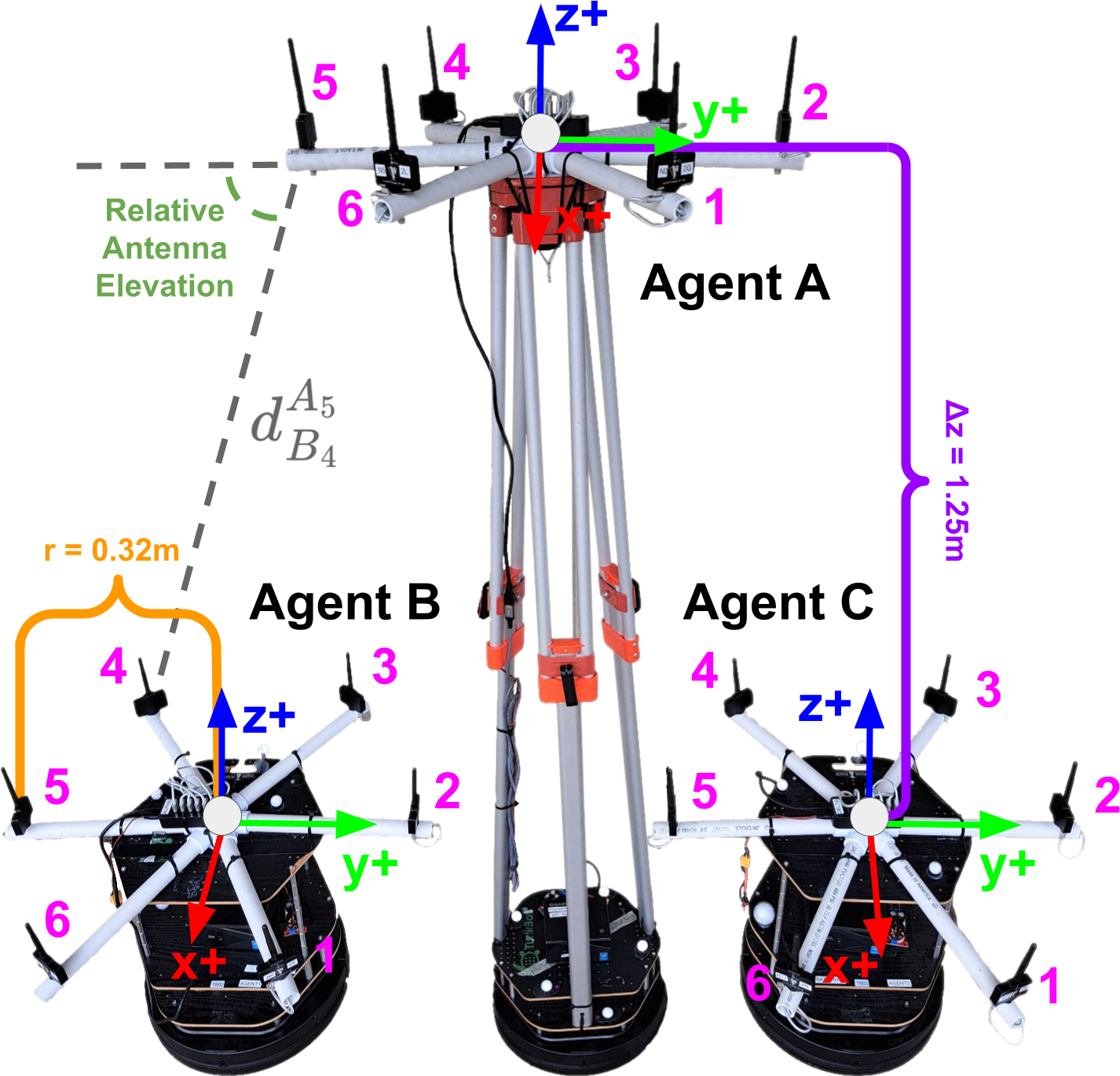
Hardware: Three agents, $A$, $B$ and $C$, were used (see Figure 3(a)). All are Turtlebot2 UGV with 6 UWB sensors evenly distributed in the $xy$-plane 0.32m from the center. Agent $A$, $B$, and $C$’s sensors are mounted 1.75m, 0.5m, and 0.5m above the ground respectively (i.e., $z^{A}_{B}=-1.25$m).

Trials: A full 22 datasets were collected with all three agents, each with 6 antennas, moving in various ways within the mocap space. Ranging measurements are performed by each pair of antennas between agents at 25Hz. Together the datasets total to nearly 6h (effectively creating over 200h of pairwise measurements). This dataset was used for Figures 2(a) and 2(b). Tables IV and IV show results for the 5 trials where all three agents are continuously moving in various arbitrary patterns with max positional and angular velocities of 1m/s and 1rad/s respectively.

Parameters: Our approach, outlined in Section V and culminating in Equation 9 and Algorithm 1, is configured as such: (1) Our mean bias correction function, $\bar{d}^{A_{i}}_{B_{j}}(\mathbf{T}^{A}_{B})$, is set to the learned 6-degree polynomial shown in Figure 2(b). This incorporates the observed mean bias with respect to elevation into our approach. (2) The current range measurements, $\tilde{d}^{A_{i}}_{B_{j}}$, and pose estimates are smoothed by a moving average filter with a 1s and 4s window length respectively. (3) Our loss function, $\ell$, is selected to be the Huber loss $\rho_{\delta}(a)$ with $\delta=0.06$. As with [20, 21, 17], Huber loss was selected due to its reduced outliers sensitivity compared to a traditional squared error loss [34]. The parameter $\delta=0.06$ was selected after doing a parameter search over our results.

Discussion of Results: Results are summarized for Absolute Position Error (APE) and Absolute Heading Error (AHE) in Figures 5(a) and 5(b) and Tables IV and IV. To demonstrate the value of individual algorithmic decisions, the tables toggles el_bias, z_fixed, Huber, where the final row represents the proposed approach. Specifically, a check indicates:

• el_bias: $\bar{d}^{A_{i}}_{B_{j}}(\mathbf{T}^{A}_{B})$ is the learned mean bias correction (see Figure 2(b)), otherwise $0$.

• z_fixed: $z$ is constrained to $z^{A}_{B}$, otherwise free.

• Huber: $\ell(a)\triangleq\rho_{0.06}(a)$, otherwise squared error loss.

The tables show the proposed approach consistently improves the mean APE by an average of 19% over the second best APE approach (i.e., without the el_bias, orange), while constraining $z$ leads to the largest APE gains. Unlike APE, there is not a clear best AHE approach. That being said, the proposed approach is only at most $1^{\circ}$ behind the best mean AHE approach for any given trial.

VII Conclusion

This work presents a UWB-ranging inter-agent relative pose estimation system that minimizes communication load. Although challenging to do a direct comparison, other state-of-the-art approaches achieve APE and AHE on the order of 0.10m and $1^{\circ}$ respectively (see Section II), but rely heavily on continuously transmitted measurements which leading to potential scaling issues with increased team size and/or decreased communication network capability By comparison, this work achieves competitive 3D results, averaged across all trials a mean APE and AHE of 0.24m and $9.5^{\circ}$ respectively, while requiring no continuously transmitted measurements. Our work outperforms the most-similar recent work [23], in part due to our learned measurement mean bias error, $\bar{d}^{A_{i}}_{B_{j}}(\mathbf{T}^{A}_{B})$, which greatly improves our APE by a average of 19% across our experimental trials. In the future, this mean bias error estimate can be further improved as a neural network – that being said, a key takeaway is that most UWB systems would benefit from a pose-dependent UWB ranging error model. Furthermore, future work will include additional flights on multiple larger drones in expansive outdoor environments and integration of this system into a larger resource-aware distributed SLAM pipeline.

References

- [1] Yulun Tian, Katherine Liu, Kyel Ok, Loc Tran, Danette Allen, Nicholas Roy, and Jonathan P. How. Search and rescue under the forest canopy using multiple uavs. Int. J. Robotics Res., 39(10-11), 2020.
- [2] Xiulong Liu, Jiannong Cao, Yanni Yang, and Shan Jiang. Cps-based smart warehouse for industry 4.0: A survey of the underlying technologies. Comput., 7(1):13, 2018.
- [3] Ali Agha, Kyohei Otsu, Benjamin Morrell, David D. Fan, Rohan Thakker, and et al. Nebula: Quest for robotic autonomy in challenging environments; TEAM costar at the DARPA subterranean challenge. CoRR, abs/2103.11470, 2021.
- [4] David Filliat and Jean-Arcady Meyer. Map-based navigation in mobile robots:: I. a review of localization strategies. Cognitive systems research, 4(4):243–282, 2003.
- [5] Muhammad Saim, Khalid Munawar, and Ubaid Al-Saggaf. An overview of localization methods for multi-agent systems. Int J Eng Res Appl, 7(01):19–24, 2017.
- [6] Xun S. Zhou and Stergios I. Roumeliotis. Robot-to-robot relative pose estimation from range measurements. IEEE Trans. Robotics, 24(6):1379–1393, 2008.
- [7] Yulun Tian, Yun Chang, Fernando Herrera Arias, Carlos Nieto-Granda, Jonathan P. How, and Luca Carlone. Kimera-Multi: Robust, Distributed, Dense Metric-Semantic SLAM for Multi-Robot Systems. IEEE Transactions on Robotics, 38(4):2022–2038, August 2022.
- [8] Wikipedia contributors. List of uwb-enabled mobile devices — Wikipedia, the free encyclopedia, 2023. [Online; accessed 8-December-2023].
- [9] Abdulrahman Alarifi, AbdulMalik S. Al-Salman, Mansour Alsaleh, Ahmad Alnafessah, Suheer Alhadhrami, Mai A. Al-Ammar, and Hend S. Al-Khalifa. Ultra wideband indoor positioning technologies: Analysis and recent advances. Sensors, 16(5):707, 2016.
- [10] Nooploop. LinkTrack – Model Selection, 2023. https://www.nooploop.com/en/linktrack/.
- [11] Nour Smaoui, Omprakash Gnawali, and Kyungki Kim. Study and mitigation of platform related UWB ranging errors. In 2020 International Conference on COMmunication Systems & NETworkS, COMSNETS 2020, Bengaluru, India, January 7-11, 2020, pages 346–353. IEEE, 2020.
- [12] Anton Ledergerber and Raffaello D’Andrea. Ultra-wideband range measurement model with gaussian processes. In IEEE Conference on Control Technology and Applications, CCTA 2017, Mauna Lani Resort, HI, USA, August 27-30, 2017, pages 1929–1934. IEEE, 2017.
- [13] Anton Ledergerber and Raffaello D’Andrea. Calibrating away inaccuracies in ultra wideband range measurements: A maximum likelihood approach. IEEE Access, 6:78719–78730, 2018.
- [14] Michael Hamer and Raffaello D’Andrea. Self-calibrating ultra-wideband network supporting multi-robot localization. IEEE Access, 6:22292–22304, 2018.
- [15] Zhiqiang Cao, Ran Liu, Chau Yuen, Achala Athukorala, Benny Kai Kiat Ng, Muraleetharan Mathanraj, and U-Xuan Tan. Relative localization of mobile robots with multiple ultra-wideband ranging measurements. In IEEE/RSJ International Conference on Intelligent Robots and Systems, IROS, pages 5857–5863, 2021.
- [16] Hao Xu, Luqi Wang, Yichen Zhang, Kejie Qiu, and Shaojie Shen. Decentralized visual-inertial-uwb fusion for relative state estimation of aerial swarm. In 2020 IEEE International Conference on Robotics and Automation, ICRA 2020, Paris, France, May 31 - August 31, 2020, pages 8776–8782. IEEE, 2020.
- [17] Hao Xu, Yichen Zhang, Boyu Zhou, Luqi Wang, Xinjie Yao, Guotao Meng, and Shaojie Shen. Omni-swarm: A decentralized omnidirectional visual-inertial-uwb state estimation system for aerial swarm. CoRR, abs/2103.04131, 2021.
- [18] Andrew Fishberg and Jonathan P. How. Multi-agent relative pose estimation with UWB and constrained communications. In IEEE/RSJ International Conference on Intelligent Robots and Systems, IROS 2022, Kyoto, Japan, October 23-27, 2022, pages 778–785. IEEE, 2022.
- [19] Kexin Guo, Xiuxian Li, and Lihua Xie. Ultra-Wideband and Odometry-Based Cooperative Relative Localization With Application to Multi-UAV Formation Control. IEEE Transactions on Cybernetics, 50(6):2590–2603, June 2020.
- [20] S. Zheng, Z. Li, Y. Liu, H. Zhang, P. Zheng, X. Liang, Y. Li, X. Bu, and X. Zou. UWB-VIO Fusion for Accurate and Robust Relative Localization of Round Robotic Teams. IEEE Robotics and Automation Letters, 7(4):11950–11957, October 2022.
- [21] Haifeng Zhang, Zhitian Li, Shuaikang Zheng, Pengcheng Zheng, Xingdong Liang, YanLei Li, Xiangxi Bu, and Xudong Zou. Range-Aided Drift-Free Cooperative Localization and Consistent Reconstruction of Multi-Ground Robots. IEEE Robotics and Automation Letters, 8(4):2094–2101, April 2023. Conference Name: IEEE Robotics and Automation Letters.
- [22] Yang Qi, Yisheng Zhong, and Zongying Shi. Cooperative 3-D relative localization for UAV swarm by fusing UWB with IMU and GPS. Journal of Physics: Conference Series, 1642(1):012028, September 2020.
- [23] Yu Xianjia, Li Qingqing, Jorge Pena Queralta, Jukka Heikkonen, and Tomi Westerlund. Cooperative UWB-Based Localization for Outdoors Positioning and Navigation of UAVs aided by Ground Robots. In 2021 IEEE International Conference on Autonomous Systems (ICAS), pages 1–5, Montreal, QC, Canada, August 2021. IEEE.
- [24] Zhiren Xun, Jian Huang, Zhehan Li, Zhenjun Ying, Yingjian Wang, Chao Xu, Fei Gao, and Yanjun Cao. CREPES: Cooperative RElative Pose Estimation System, March 2023. arXiv:2302.01036 [cs].
- [25] Abhishek Goudar, Timothy D. Barfoot, and Angela P. Schoellig. Continuous-Time Range-Only Pose Estimation, May 2023. arXiv:2304.09043 [cs].
- [26] Adyasha Mohanty, Asta Wu, Sriramya Bhamidipati, and Grace Gao. Precise relative positioning via tight-coupling of gps carrier phase and multiple uwbs. IEEE Robotics and Automation Letters, 7(2):5757–5762, 2022.
- [27] Weisong Wen, Xiwei Bai, Guohao Zhang, Shengdong Chen, Feng Yuan, and Li-Ta Hsu. Multi-agent collaborative gnss/camera/ins integration aided by inter-ranging for vehicular navigation in urban areas. IEEE Access, 8:124323–124338, 2020.
- [28] Xianjia Yu, Qingqing Li, Jorge Peña Queralta, Jukka Heikkonen, and Tomi Westerlund. Applications of UWB networks and positioning to autonomous robots and industrial systems. In 10th Mediterranean Conference on Embedded Computing, MECO 2021, Budva, Montenegro, June 7-10, 2021, pages 1–6. IEEE, 2021.
- [29] Harry B Lee et al. Accuracy limitations of range-range (spherical) multilateration systems. Technical report, Lincoln Laboratory, 1973.
- [30] Berthold K. P. Horn. Closed-form solution of absolute orientation using unit quaternions. JOSA A, 4(4):629–642, April 1987. Publisher: Optica Publishing Group.
- [31] Richard B. Langley. Dilution of Precision, May 1999.
- [32] Timothy D Barfoot. State estimation for robotics. Cambridge University Press, 2017.
- [33] Rue Henri Fabre. TeraRanger Evo 15m Specification Sheet, 2021.
- [34] Richard Hartley and Andrew Zisserman. Multiple view geometry in computer vision. Cambridge university press, 2003.