SC-GS: Sparse-Controlled Gaussian Splatting for Editable Dynamic Scenes

Abstract

Novel view synthesis for dynamic scenes is still a challenging problem in computer vision and graphics. Recently, Gaussian splatting has emerged as a robust technique to represent static scenes and enable high-quality and real-time novel view synthesis. Building upon this technique, we propose a new representation that explicitly decomposes the motion and appearance of dynamic scenes into sparse control points and dense Gaussians, respectively. Our key idea is to use sparse control points, significantly fewer in number than the Gaussians, to learn compact 6 DoF transformation bases, which can be locally interpolated through learned interpolation weights to yield the motion field of 3D Gaussians. We employ a deformation MLP to predict time-varying 6 DoF transformations for each control point, which reduces learning complexities, enhances learning abilities, and facilitates obtaining temporal and spatial coherent motion patterns. Then, we jointly learn the 3D Gaussians, the canonical space locations of control points, and the deformation MLP to reconstruct the appearance, geometry, and dynamics of 3D scenes. During learning, the location and number of control points are adaptively adjusted to accommodate varying motion complexities in different regions, and an ARAP loss following the principle of as rigid as possible is developed to enforce spatial continuity and local rigidity of learned motions. Finally, thanks to the explicit sparse motion representation and its decomposition from appearance, our method can enable user-controlled motion editing while retaining high-fidelity appearances. Extensive experiments demonstrate that our approach outperforms existing approaches on novel view synthesis with a high rendering speed and enables novel appearance-preserved motion editing applications. Project page: https://yihua7.github.io/SC-GS-web/

*Equal Contribution $\dagger$Corresponding Author

1 Introduction

Novel view synthesis from a monocular video is a crucial problem with many applications in virtual reality, gaming, and the movie industry. However, extracting scene geometry and appearance from limited observations  [23, 41, 24] is challenging. Concurrently, real-world scenes often contain dynamic objects, which pose additional challenges in representing object movements accurately to reflect real-world dynamics [30, 15, 26, 27, 14].

Recent advancements in this area are primarily driven by neural radiance fields (NeRF)  [23, 1, 41, 2, 3], which utilizes an implicit function to simultaneously learn scene geometry and appearance from multi-view images. Various approaches have been proposed to model dynamic objects by predicting scene flows [30, 15, 43, 38, 6, 26, 27, 11, 16] leveraging plane- or volume grid-based representations [31, 4, 33, 20, 7] and temporal interpolation [14, 28]. Despite significant progress, NeRF-based representations still struggle with low rendering qualities, speeds, and high memory usage. This issue is particularly evident when rendering at high resolutions [50, 8, 24], as they necessitate sampling hundreds of query points along each ray to predict color and opacity for rendering a single pixel.

Most recently, Gaussian splatting [12], which represents a scene as 3D Gaussians, has shown remarkable performance in terms of rendering quality, resolution, and speed. Utilizing a point-based scene representation, this method rasterizes 3D Gaussians to render images from specified views. It enables fast model training and real-time inference, achieving state-of-the-art (SOTA) visual quality. However, its existing formulation only applies to static scenes. It remains a challenge to incorporate object motion into the Gaussian representation without compromising rendering quality and speed. An intuitive method [47] involves learning a flow vector for each 3D Gaussian. While this method can yield high-quality rendering results, it incurs a significant time cost for training and inference. Moreover, modeling motion in such a high-dimensional space leads to noisy trajectories and poor generalization in novel views, as demonstrated in Fig. 6 (a).

Motivated by the observation that real-world motions are often sparse, spatially continuous, and locally rigid, we propose an approach to enrich Gaussian splatting with learnable sparse control points ($\approx$512) compared to the number of Gaussians ($\approx$100K), in a much more compact space for modeling scene dynamics. These control points are associated with time-varying 6 DoF transformations parameterized as rotation using quaternion and translation parameters, which can be locally interpolated through learned interpolation weights to yield the motion field of dense Gaussians. Instead of directly optimizing 6 DoF parameters for each control point, we utilize an MLP conditioned on time and location to predict them. This strategy reduces learning complexities, enhances model capabilities, and provides motions with improved spatial and temporal continuity and coherence. Then, we jointly learn the canonical space 3D Gaussian parameters, locations, and radius of sparse control points at canonical space and the MLP to predict their time-varying transformations from a monocular video for dynamic novel view synthesis. During learning, we introduce an adaptive strategy to adaptively change the number of sparse points to accommodate motion complexities in different regions and employ an ARAP loss that encourages the learned motions to be locally as rigid as possible.

Owing to the effective motion and appearance representations, our approach simultaneously enables high-quality dynamic view synthesis and motion editing, as shown in Fig. 1. We perform extensive experiments and ablation studies on benchmark datasets, demonstrating that our model surpasses existing methods both quantitatively and qualitatively while maintaining high rendering speeds. Furthermore, by learning a control graph from the scene motion, our control points-based motion representation allows for convenient motion editing, a feature not present in existing methods  [30, 7, 4, 31, 11]. More results for motion editing are included in Fig. 5 and the supplementary material. Our contributions can be summarized as follows:

• We introduce sparse control points together with an MLP for modeling scene motion, based on the insight that motions within a scene can be represented by a compact subspace with a sparse set of bases.

• We employ adaptive learning strategies and design a regularization loss based on rigid constraints to enable effective learning of appearances, geometry, and motion from a monocular video.

• Thanks to the sparse motion representation, our approach enables motion editing by manipulating the learned control points while maintaining high-fidelity appearances.

• Extensive experiments show our approach achieves SOTA performance quantitatively and qualitatively.

2 Related Work

Dynamic NeRF. Novel view synthesis has been a prominent topic in the academic field for several years. NeRF [23] models static scenes implicitly with MLPs, and many works [30, 15, 43, 38, 26, 27, 11] have expanded its usage to dynamic scenes via a deformation field. Some methods [9, 14, 28] represent dynamic scenes as 4D radiance fields but face extensive computational costs due to ray point sampling and volume rendering. Several acceleration approaches have been used for dynamic scene modeling. DeVRF [20] introduces a grid representation, and IBR-based methods [18, 16, 17, 45] use multi-camera information for quality and efficiency. Other methods used primitives [21], predicted MLP maps [29], or grid/plane-based structures [33, 7, 4, 31, 39, 40] for speed and performance in various dynamic scenes. However, hybrid models under perform with high-rank dynamic scenes due to their low-rank assumption.

Dynamic Gaussian Splatting. Gaussian Splatting [12] offers improved rendering quality and speed for radiance fields. Several concurrent works have adapted 3D Gaussians for dynamic scenes. Luiten et al. [22] utilizes frame-by-frame training, suitable for multi-view scenes. Yang et al. [47] separate scenes into 3D Gaussians and a deformation field for monocular scenes but face slow training due to an extra MLP for learning Gaussian offsets. Following [47], Wu et al. [42] replaced the MLP with multi-resolution hex-planes [4] and a lightweight MLP. Yang et al. [48] include time as an additional feature in 4D Gaussians but face quality issues compared to constraints in canonical space. Our work proposes using sparse control points to drive the deformation of 3D Gaussians, which enhances rendering quality and reduces MLP query overhead. The learned control point graph can also be used for motion editing.

3D Deformation and Editing. Traditional deformation methods in computer graphics are typically based on Laplacian coordinates [19, 36, 35, 34], Poisson equation [51] and cage-based approaches [49, 54]. These methods primarily focus on preserving the geometric details of 3D objects during the deformation process. In recent years, there have been other approaches [52, 44] that aim to edit the scene geometry learned from 2D images. These methods prioritize the rendering quality of the edited scene. Our approach falls into this category. However, instead of relying on the implicit and computationally expensive NeRF-based approach, our method employs an explicit point-based control graph deformation strategy and Gaussian rendering, which is more intuitive and efficient.

Figure 2: We present a novel method of employing sparse control points and a deformation MLP to direct 3D Gaussian dynamics. The MLP uses canonical control point coordinates and time to obtain per-control-point 6-DOF transformations, which guide 3D Gaussian deformation based on K nearest control points. Transformed Gaussians can then be rendered into images, and rendering loss calculated, before backpropagating gradients to optimize the Gaussians, control points, and MLP. Gaussian and control point density are adaptively managed during training.

3 Preliminaries

Gaussian splatting represents a 3D scene using colored 3D Gaussians [12]. Each Gaussian $G$ has a 3D center location $\mu$ and a 3D covariance matrix $\Sigma$,

$$G(x)=e^{-\frac{1}{2}(x-\mu)^{T}\Sigma^{-1}(x-\mu)}.$$ (1)

The covariance matrix $\Sigma$ is decomposed as $\Sigma=RSS^{T}R^{T}$ for optimization, with $R$ as a rotation matrix represented by a quaternion $q\in\mathbf{SO}(3)$, and $S$ as a scaling matrix represented by a 3D vector $s$. Each Gaussian has an opacity value $\sigma$ to adjust its influence in rendering and is associated with sphere harmonic (SH) coefficients $sh$ for view-dependent appearance. A scene is parameterized as a set of Gaussians $\mathcal{G}=\{G_{j}:\mu_{j},q_{j},s_{j},\sigma_{j},sh_{j}\}$.

Rendering an image involves projecting these Gaussians onto the 2D image plane and aggregating them using fast $\alpha$-blending. The 2D covariance matrix and center are $\Sigma^{\prime}=JW\Sigma W^{T}J^{T}$ and $\mu^{\prime}=JW\mu$. The color $C(u)$ of a pixel $u$ is rendered using a neural point-based $\alpha$-blending as,

$$\small C({u})=\sum_{i\in N}T_{i}\alpha_{i}\mathcal{SH}(sh_{i},v_{i}),\text{ where }T_{i}=\Pi_{j=1}^{i-1}(1-\alpha_{j}).$$ (2)

Here, $\mathcal{SH}$ is the spherical harmonic function and $v_{i}$ is the view direction. $\alpha_{i}$ is calculated by evaluating the corresponding projected Gaussian $G_{i}$ at pixel $u$ as,

$$\alpha_{i}=\sigma_{i}e^{-\frac{1}{2}({p}-\mu_{i}^{\prime})^{T}\Sigma_{i}^{\prime}({p}-\mu_{i}^{\prime})},$$ (3)

where $\mu_{i}^{\prime}$ and $\Sigma_{i}^{\prime}$ are the center point and covariance matrix of Gaussian $G_{i}$, respectively. By optimizing the Gaussian parameters $\{G_{j}:\mu_{j},q_{j},s_{j},\sigma_{j},c_{j}\}$ and adjusting Gaussian density adaptively, high-quality images can be synthesized in real-time. We further introduce sparse control points to adapt Gaussian splatting for dynamic scenes while maintaining rendering quality and speed.

4 Method

Our goal is to reconstruct a dynamic scene from a monocular video. We represent the geometry and appearance of the dynamic scene using Gaussians in the canonical space while modeling the motion through a set of control points together with time-varying 6DoF transformations predicted by an MLP. These learned control points and corresponding transformations can be utilized to drive the deformation of Gaussians across different timesteps. The number of control points is significantly smaller than that of Gaussians, resulting in a set of compact motion bases for modeling scene dynamics and further facilitating motion editing. An overview of our method is shown in Fig. 2. In the following, we first present the sparse control points for representing compact motion bases in Sec. 4.1, followed by the dynamic scene rendering formulation in Sec. 4.2 and optimization process in Sec. 4.3.

4.1 Sparse Control Points

To derive a compact motion representation, we introduce a set of sparse control points $\mathcal{P}=\{(p_{i}\in\mathbb{R}^{3},o_{i}\in\mathbb{R}^{+})\},i\in\{1,2,\cdots,N_{p}\}$. Here, $p_{i}$ denotes the learnable coordinate of control point $i$ in the canonical space. $o_{i}$ is the learnable radius parameter of a radial-basis-function (RBF) kernel that controls how the impact of a control point on a Gaussian will decrease as their distances increase. $N_{p}$ is the total number of control points, which is considerably fewer than that of Gaussians.

For each control point $k$, we learn time-varying 6 DoF transformations $[R_{i}^{t}|T_{i}^{t}]\in\mathbf{SE}(3)$ , consisting of a local frame rotation matrix $R_{i}^{t}\in\mathbf{SO}(3)$ and a translation vector $T_{i}^{t}\in\mathbb{R}^{3}$. Instead of directly optimizing the transformation parameters for each control point at different time steps, we employ an MLP $\Psi$ to learn a time-varying transformation field and query the transformation of each control point $p_{k}$ at each timestep $t$ as:

$$\Psi:(p_{i},t)\rightarrow(R_{i}^{t},T_{i}^{t}).$$ (4)

Note that in practical implementations, $R_{i}^{t}$ is represented equivalently as a quaternion $r_{i}^{t}$ for more stable optimization and convenient interpolation for generating the motions of Gaussians in the follow-up steps.

4.2 Dynamic Scene Rendering

Equipped with the time-varying transformation parameters $(R_{i}^{t},T_{i}^{t})$ for sparse control points which form a set of compact motion bases, the next step is to determine the transformation of each Gaussian at different time steps to derive the motion of the entire scene. We derive the dense motion field of Gaussians using linear blend skinning (LBS) [37] by locally interpolating the transformations of their neighboring control points. Specifically, for each Gaussian $G_{j}:(\mu_{j},q_{j},s_{j},\sigma_{j},sh_{j})$, we use k-nearest neighbor (KNN) search to obtain its $K(=4)$ neighboring control points denoted as $\{p_{k}|k\in\mathcal{N}_{j}\}$ in canonical space. Then, the interpolation weights for control point $p_{k}$ can be computed with Gaussian-kernel RBF [10, 5, 25] as:

$$\small w_{jk}=\frac{\hat{w}_{jk}}{\sum\limits_{k\in\mathcal{N}_{j}}\hat{w}_{jk}}\text{, where }\ \hat{w}_{jk}=\text{exp}(-\frac{d_{jk}^{2}}{2o_{k}^{2}}),$$ (5)

where $d_{jk}$ is the distance between center of Gaussian $G_{j}$ and the neighboring control point $p_{k}$, and $o_{k}$ is the learned radius parameter of $p_{k}$. During training, these interpolation weights are adaptable to model complex motions by encouraging the learnable radius parameters to be optimized in a way that can accurately reconstruct the video frames.

Using the interpolation weights of neighboring control points, we can calculate a Gaussian motion field through interpolation. Following dynamic fusion works [25, 13, 5], we employ LBS [37] to compute the warped Gaussian $\mu_{j}^{t}$ and $q_{j}^{t}$ as Eq. (6) and Eq. (7) for simplicity and efficiency:

$$\mu_{j}^{t} =\sum\limits_{k\in\mathcal{N}_{j}}w_{jk}\left(R_{k}^{t}(\mu_{j}-p_{k})+p_{k}+T_{k}^{t}\right),$$ (6)

$$q_{j}^{t} =(\sum\limits_{k\in\mathcal{N}_{j}}w_{jk}r_{k}^{t})\otimes q_{j},$$ (7)

where $R_{k}^{t}\in\mathbb{R}^{3\times 3}$ and $r_{k}^{t}\in\mathbb{R}^{4}$ are the matrix and quaternion representations of predicted rotation on control point $k$ respectively. $\otimes$ is the production of quaternions, obtaining the quaternion of the composition of corresponding rotation transforms. Then, with the updated Gaussian parameters, we are able to perform rendering at time step $t$ following Eq. (2) and Eq. (3).

4.3 Optimization

Our dynamic scene representation consists of control points $\mathcal{P}$ and Gaussians $G$ in the canonical space and the deformation MLP $\Psi$. To stabilize the training process, we first pre-train $\mathcal{P}$ and $\Psi$ to model the coarse scene motion with the Gaussians $\mathcal{G}$ fixed. The details are included in the supplementary material. Then, the whole model is optimized jointly. To facilitate learning, we introduce an ARAP loss to encourage the learned motion of control points to be locally rigid and employ an adaptive density adjustment strategy to adapt to varying motion complexities in different areas.

ARAP Loss and Overall Optimization Objective. To avoid local minima and regularize the unstructured control points, we introduce an ARAP loss $\mathcal{L}_{\text{arap}}$ that encourages their motions to be locally rigid, following the principle of being as rigid as possible [34]. Before computing the ARAP loss for control points, it is necessary to identify the edges that connect them. To avoid linking unrelated points, we opt to connect the points that have closely aligned trajectories in the scene motion. Specifically, for a control point $p_{j}$, we firstly calculate its trajectory $p_{i}^{\text{traj}}$ that includes its locations across $N_{t}(=8)$ randomly sampled time steps as:

$$p_{i}^{\text{traj}}=\frac{1}{N_{t}}p_{i}^{t_{1}}\oplus p_{i}^{t_{2}}\oplus\cdots\oplus p_{i}^{t_{N_{t}}},$$ (8)

where $\oplus$ denotes vector concatenation operation. Based on the trajectories obtained, we perform ball queries and use all control points $\mathcal{N}_{c_{i}}$ within a pre-defined radius to define a local area. Then, to calculate $\mathcal{L}_{\text{arap}}$, we randomly sample two time steps $t_{1}$ and $t_{2}$. For each point $p_{k}$ within the radius (i.e. $k\in\mathcal{N}_{c_{i}}$), its transformed locations with learned translation parameters $T_{k}^{t_{1}}$ and $T_{k}^{t_{2}}$ are: $p_{k}^{t_{1}}=p_{k}+T_{k}^{t_{1}}$ and $p_{k}^{t_{2}}=p_{k}+T_{k}^{t_{2}}$, thus the rotation matrix $\hat{R}_{i}$ can be estimated following a rigid motion assumption [34] as:

$$\small\hat{R}_{i}=\operatorname*{arg\,min}\limits_{R\in\mathbf{SO}(3)}\sum_{k\in\mathcal{N}_{c_{i}}}{w}_{ik}||(p_{i}^{t_{1}}-p_{k}^{t_{1}})-{R}(p_{i}^{t_{2}}-p_{k}^{t_{2}})||^{2}.$$ (9)

Here $w_{ik}$ is calculated similarly to $w_{jk}$ in Eq. (5) by replacing Gaussian position $\mu_{j}$ with control point position $p_{i}$, which weights the contribution of different neighboring points $p_{k}$ according to their impact on $p_{i}$. Eq. (9) can be easily solved using SVD decomposition according to [34]. Then, $\mathcal{L}_{\text{arap}}$ is designed as,

$$\footnotesize\mathcal{L}_{\text{arap}}(p_{i},t_{1},t_{2})=\sum_{k\in\mathcal{N}_{c_{i}}}{w}_{ik}||(p_{i}^{t_{1}}-p_{k}^{t_{1}})-\hat{R}_{i}(p_{i}^{t_{2}}-p_{k}^{t_{2}})||^{2},$$ (10)

which evaluates the degree to which the learned motion deviates from the assumption of local rigidity. By penalizing $\mathcal{L}_{\text{arap}}$, the learned motions are encouraged to be locally rigid. The rigid regularization significantly enhances the learned motion with visualizations shown in Fig. 6.

For optimization, besides $L_{\text{arap}}$, the rendering loss $\mathcal{L}_{\text{render}}$ is derived by comparing the rendered image at different time steps with ground truth reference images using a combination of $\mathcal{L}_{1}$ loss and D-SSIM loss following [12]. Finally, the overall loss is constructed as: $\mathcal{L}=\mathcal{L}_{\text{render}}+\mathcal{L}_{\text{arap}}$.

Table 1: Quantitative comparison on D-NeRF [30] datasets. We present the average PSNR/SSIM/LPIPS (VGG) values for novel view synthesis on dynamic scenes from D-NeRF, with each cell colored to indicate the best, second best, and third best.

Methods	Hook			Jumpingjacks			Trex			BouncingBalls
	PSNR($\uparrow$)	SSIM($\uparrow$)	LPIPS($\downarrow$)	PSNR($\uparrow$)	SSIM($\uparrow$)	LPIPS($\downarrow$)	PSNR($\uparrow$)	SSIM($\uparrow$)	LPIPS($\downarrow$)	PSNR($\uparrow$)	SSIM($\uparrow$)	LPIPS($\downarrow$)
D-NeRF [30]	29.25	.968	.1120	32.80	.981	.0381	31.75	.974	.0367	38.93	.987	.1074
TiNeuVox-B [7]	31.45	.971	.0569	34.23	.986	.0383	32.70	.987	.0340	40.73	.991	.0472
Tensor4D [33]	29.03	.955	.0499	24.01	.919	.0768	23.51	.934	.0640	25.36	.961	.0411
K-Planes [31]	28.59	.953	.0581	32.27	.971	.0389	31.41	.980	.0234	40.61	.991	.0297
FF-NVS [11]	32.29	.980	.0400	33.55	.980	.0300	30.71	.960	.0400	40.02	.990	.0400
4D-GS [42]	30.99	.990	.0248	33.59	.990	.0242	32.16	.988	.0216	38.59	.993	.0267
Baseline	34.47	.990	.0195	35.74	.992	.0178	36.37	.994	.0103	41.45	.996	.0190
Ours	39.87	.997	.0076	41.13	.998	.0067	41.24	.998	.0046	44.91	.998	.0166

Methods	Hellwarrior			Mutant			Standup			Average
	PSNR($\uparrow$)	SSIM($\uparrow$)	LPIPS($\downarrow$)	PSNR($\uparrow$)	SSIM($\uparrow$)	LPIPS($\downarrow$)	PSNR($\uparrow$)	SSIM($\uparrow$)	LPIPS($\downarrow$)	PSNR($\uparrow$)	SSIM($\uparrow$)	LPIPS($\downarrow$)
D-NeRF [30]	25.02	.955	.0633	31.29	.978	.0212	32.79	.983	.0241	31.69	.975	.0575
TiNeuVox-B [7]	28.17	.978	.0706	33.61	.982	.0388	35.43	.991	.0230	33.76	.983	.0441
Tensor4D [33]	31.40	.925	.0675	29.99	.951	.0422	30.86	.964	.0214	27.62	.947	.0471
K-Planes [31]	25.27	.948	.0775	33.79	.982	.0207	34.31	.984	.0194	32.32	.973	.0382
FF-NVS [11]	27.71	.970	.0500	34.97	.980	.0300	36.91	.990	.0200	33.73	.979	.0357
4D-GS [42]	31.39	.974	.0436	35.98	.996	.0120	35.37	.994	.0136	34.01	.987	.0316
Baseline	39.07	.982	.0350	41.45	.998	.0045	41.04	.996	.0071	38.51	.992	.0162
Ours	42.93	.994	.0155	45.19	.999	.0028	47.89	.999	.0023	43.31	.997	.0063

Adaptive Control Points. Following [12], we also develop an adaptive density adjustment strategy to add and prune control points, which adjusts their distributions for modeling varying motion complexities, e.g. areas that exhibit complex motion patterns typically require control points of high densities. 1) To determine whether a control point $p_{i}$ should be pruned, we calculate its overall impact $W_{i}=\sum_{j\in\tilde{\mathcal{N}}_{i}}w_{ji}$ on the set of Gaussians $j\in\tilde{\mathcal{N}}_{i}$ whose K nearest neighbors include $p_{i}$. Then, we prune $p_{i}$ if $W_{i}$ is close to zero, indicating little contribution to the motion of 3D Gaussians. 2) To determine whether a control point $p_{k}$ should be cloned, we calculate the summation of Gaussian gradient norm with respect to Gaussians in set $\tilde{\mathcal{N}}_{k}$ as:

$$\small g_{i}=\sum\limits_{j\in\tilde{\mathcal{N}}_{i}}\tilde{w}_{j}||\frac{d\mathcal{L}}{d\mu_{j}}||^{2}_{2}\text{, where }\tilde{w}_{j}=\frac{w_{ji}}{\sum\limits_{j\in\tilde{\mathcal{N}}_{k}}w_{ji}}.$$ (11)

A large $g_{k}$ indicates poor reconstructions. Therefore, we clone $p_{k}$ and add a new control point $p^{\prime}_{k}$ to the expected position of related Gaussians to improve the reconstruction:

$$p^{\prime}_{k}=\sum\limits_{j\in\tilde{\mathcal{N}}_{k}}\tilde{w}_{i}\mu_{j};\ \sigma^{\prime}_{k}=\sigma_{k}.$$ (12)

5 Motion Editing

Since our approach utilizes an explicit and sparse motion representation, it further allows for efficient and intuitive motion editing through the manipulation of control points. It is achieved by predicting the trajectory of each control point across different time steps, determining their neighborhoods, constructing a rigid control graph, and performing motion editing by graph deformation.

Control Point Graph. With the trained control points $\mathcal{P}$ and the MLP $\Psi$, we construct a control point graph $\mathcal{G}$ that connects control points based on their trajectories. For each vertex of the graph, i.e., control point $p_{i}$, we firstly calculate its trajectory $p_{i}^{\text{traj}}$ derived from Eq. (8). Then, the vertex is connected with other vertices that fall within a ball of a pre-determined radius parameter based on $p_{i}^{\text{traj}}$. The edge weights $w_{ij}$ between two connected vertices $p_{i}$ and $p_{j}$ are calculated using Eq. (5). Building the control graph based on point trajectory helps take into account the overall motion sequence instead of a single timestep, which avoids unreasonable edge connections. We demonstrate the advantage of this choice in the supplementary material.

Motion Editing. In order to maintain the local rigidity, we perform ARAP [34] deformation on the control graph based on constraints specified by users. Mathematically, given a set of user-defined handle points $\{h_{l}\in\mathbb{R}^{3}\ |l\in\mathcal{H}\subset\{1,2,\cdots,N_{p}\}\}$, the control graph $\mathcal{P}^{\prime}$ can be deformed by minimizing the APAR energy formulated as:

$$\small E(\mathcal{P}^{\prime})=\sum\limits_{i=1}^{N_{p}}\sum\limits_{j\in{\mathcal{N}}_{i}}{w}_{ij}||(p_{i}^{\prime}-p_{j}^{\prime})-\hat{R}_{i}(p_{i}-p_{j})||^{2},$$ (13)

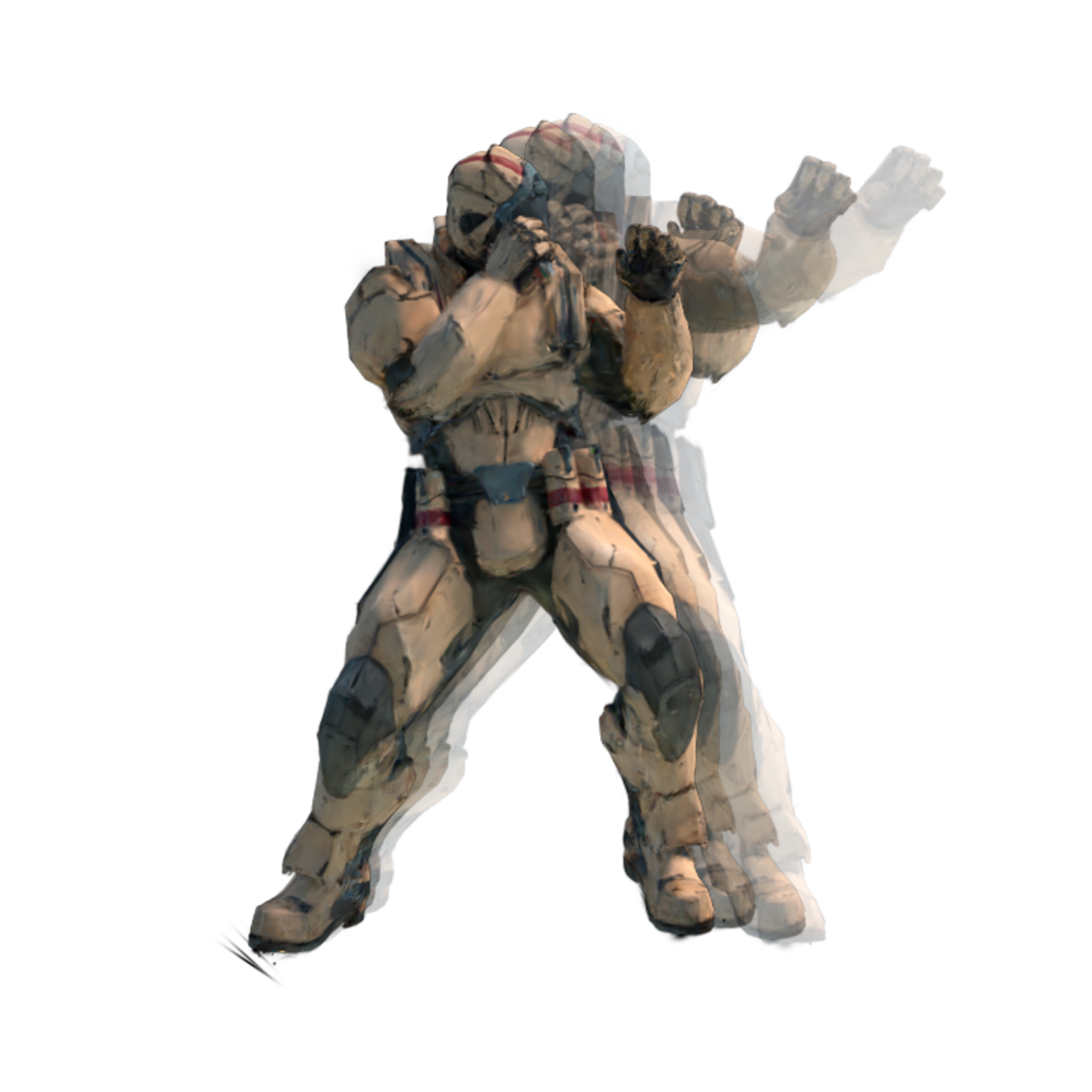
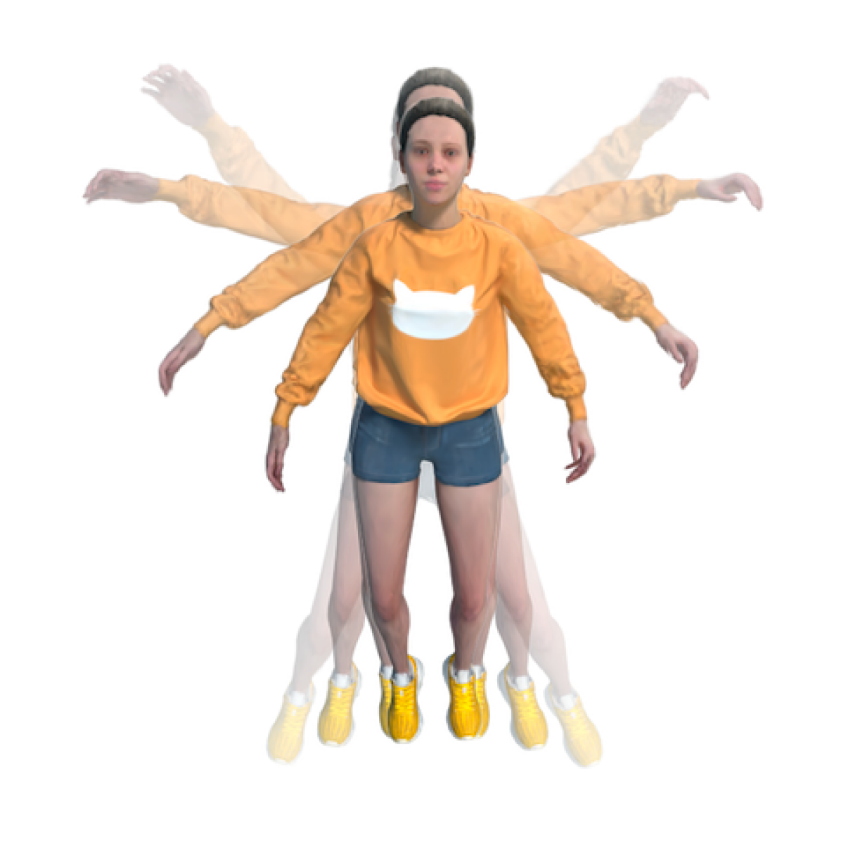
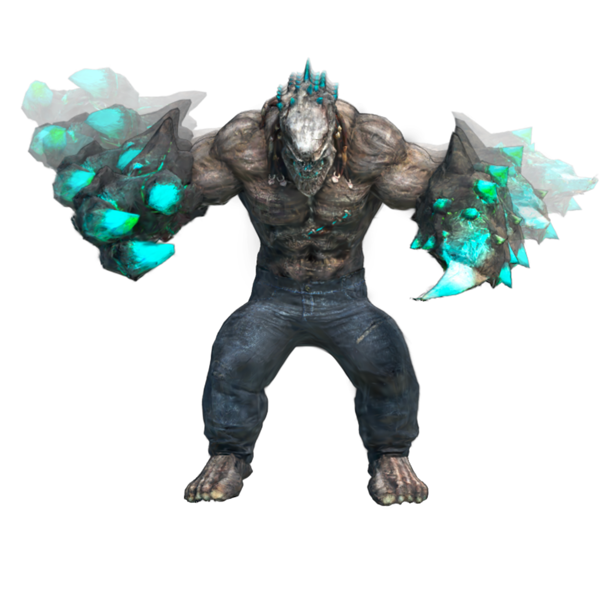
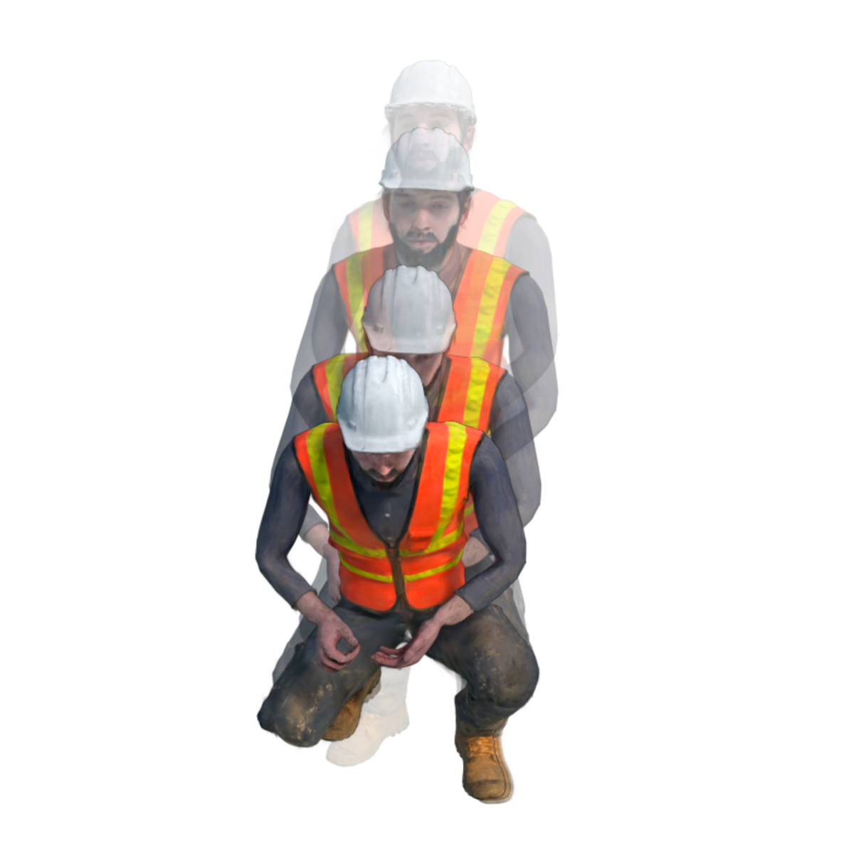
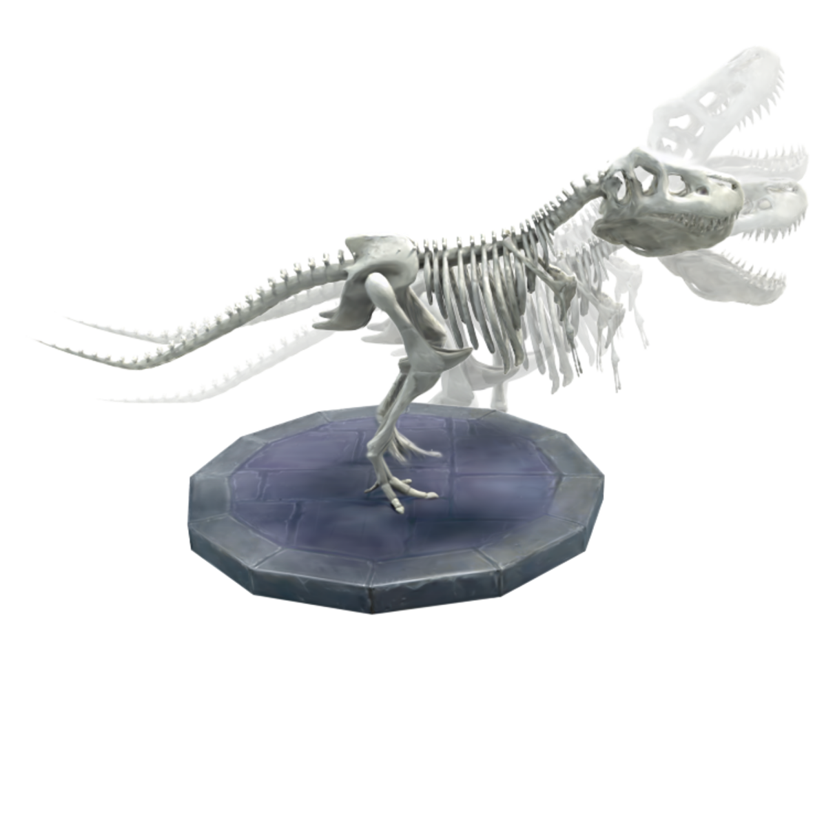
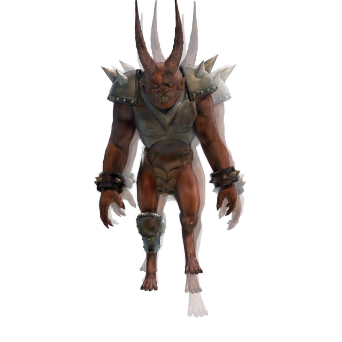
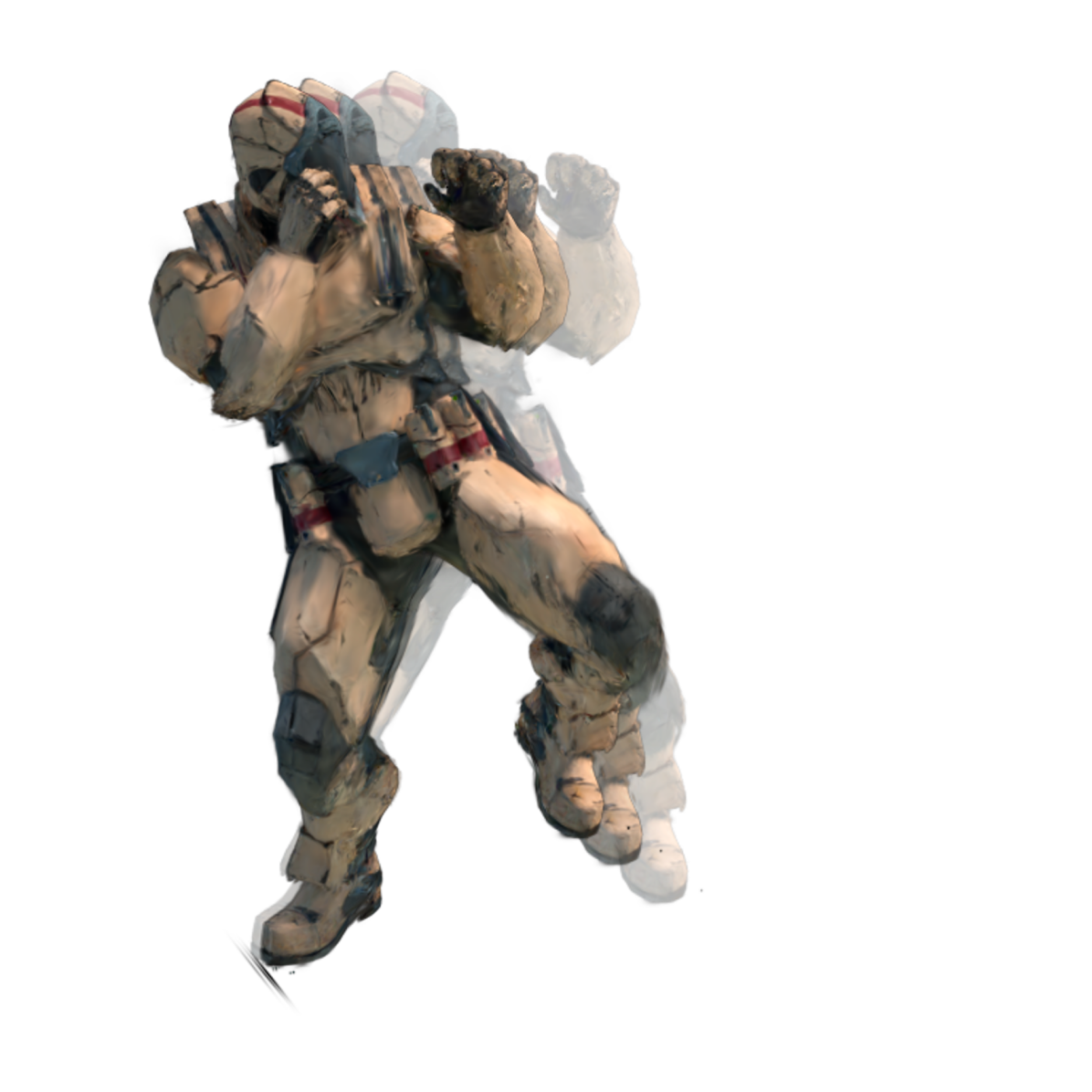
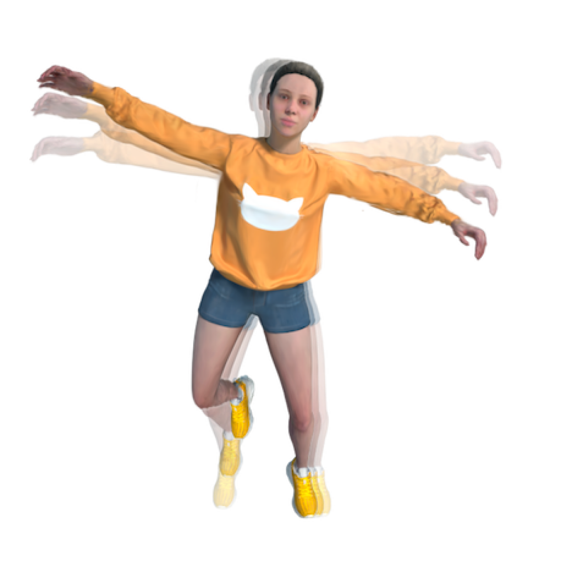
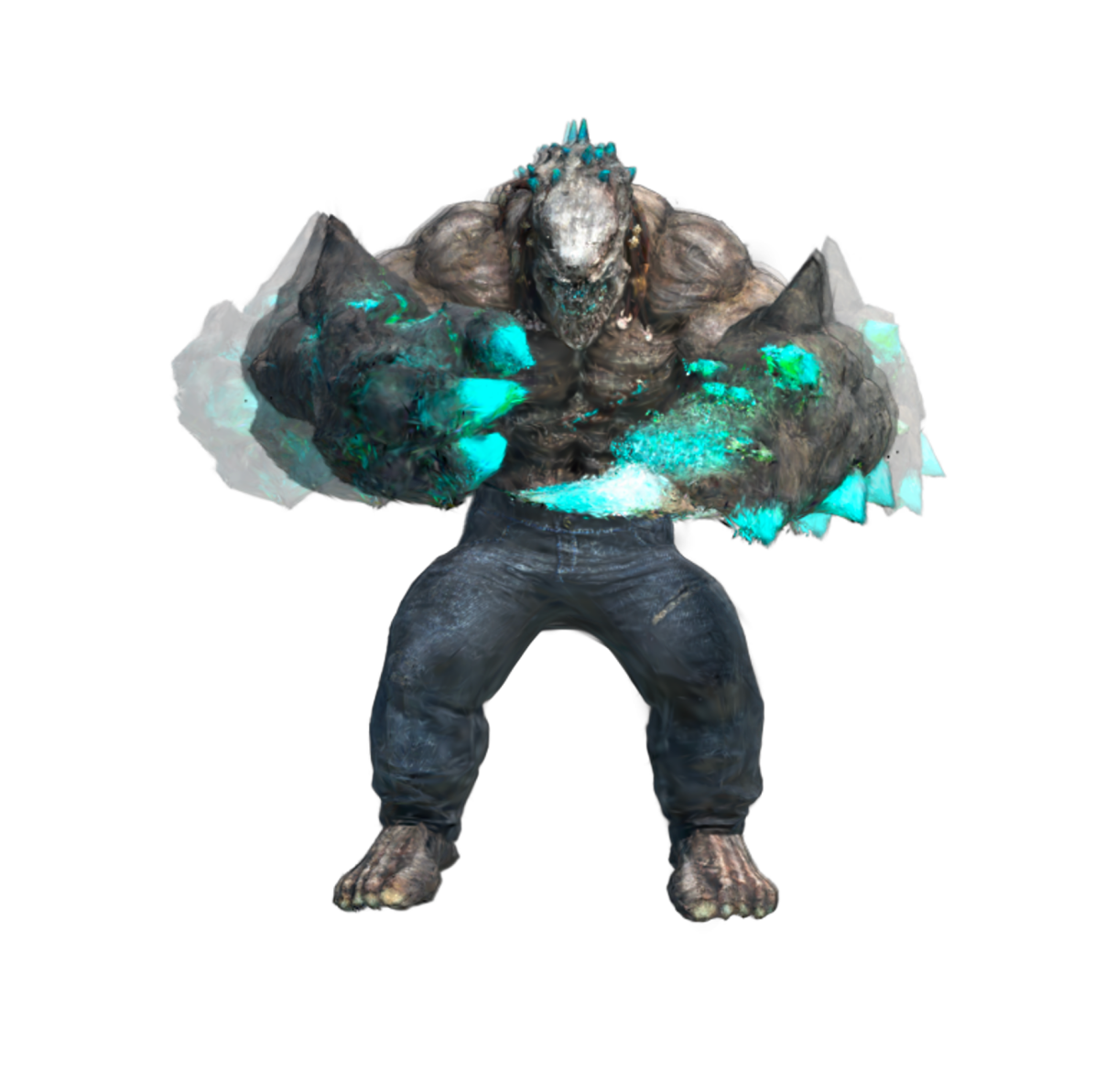
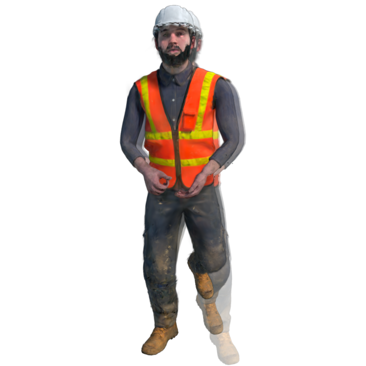
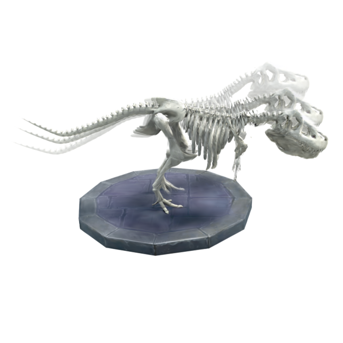
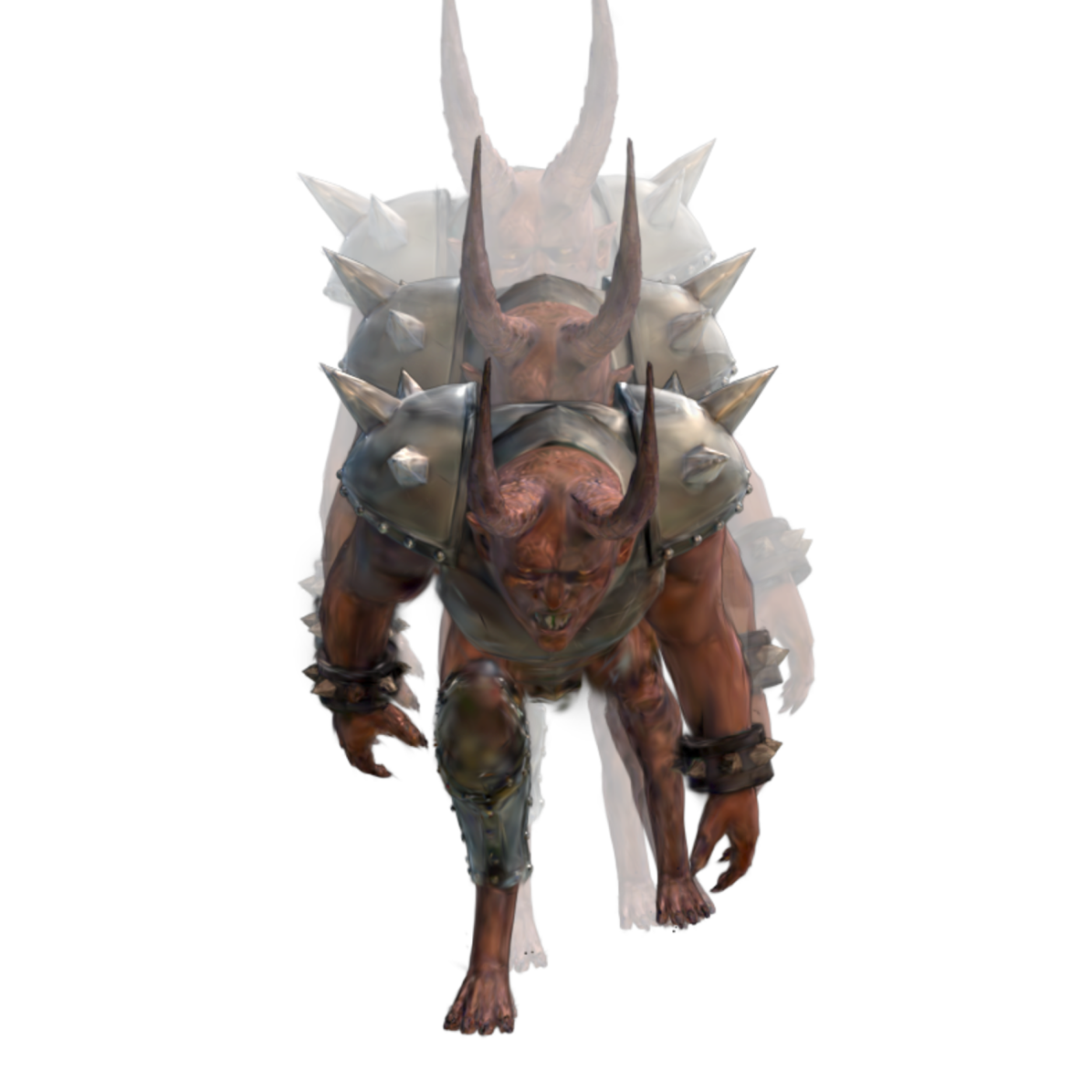
with the fixed position condition $p_{l}^{\prime}=h_{l}$ for $l\in\mathcal{H}$. Here $\hat{R}_{i}$ is the rigid local rotation defined on each control point. This optimization problem can be efficiently solved by alternately optimizing local rotations $\hat{R}_{i}$ and deformed control point positions $p^{\prime}$. We refer the readers to  [34] for the specific optimization process. The solved rotation $\hat{R}_{i}$ and translation $\hat{T}_{i}=p_{i}^{\prime}-p_{i}$ form a 6 DoF transformation for each control point, which is consistent with our motion representation. Thus, Gaussians can be warped by the deformed control points by simply replacing the transformation in Eq. (6) and Eq. (7), which can be rendered into high-quality edited images even for motion out of the training sequence. We visualize the motion editing results in Fig. 5.

Table 2: Quantitative comparison on NeRF-DS [46] datasets. We display the average PSNR/MS-SSIM/LPIPS (Alex) metrics for novel view synthesis on dynamic scenes from NeRF-DS, with each cell colored to indicate the best, second best, and third best.

Methods	Bell			Sheet			Press			Basin
	PSNR($\uparrow$)	MS-SSIM($\uparrow$)	LPIPS($\downarrow$)	PSNR($\uparrow$)	MS-SSIM($\uparrow$)	LPIPS($\downarrow$)	PSNR($\uparrow$)	MS-SSIM($\uparrow$)	LPIPS($\downarrow$)	PSNR($\uparrow$)	MS-SSIM($\uparrow$)	LPIPS($\downarrow$)
HyperNeRF [27]	24.0	.884	.159	24.3	.874	.148	25.4	.873	.164	20.2	.829	.168
NeRF-DS [46]	23.3	.872	.134	25.7	.918	.115	26.4	.911	.123	20.3	.868	.127
TiNeuVox-B [7]	23.1	.876	.113	21.1	.745	.234	24.1	.892	.133	20.7	.896	.105
Baseline	24.9	.917	.124	26.1	.903	.127	25.1	.884	.221	19.6	.852	.144
Ours	25.1	.918	.117	26.2	.898	.142	26.6	.901	.135	19.6	.846	.154
Methods	Cup			Sieve			Plate			Average
	PSNR($\uparrow$)	MS-SSIM($\uparrow$)	LPIPS($\downarrow$)	PSNR($\uparrow$)	MS-SSIM($\uparrow$)	LPIPS($\downarrow$)	PSNR($\uparrow$)	MS-SSIM($\uparrow$)	LPIPS($\downarrow$)	PSNR($\uparrow$)	MS-SSIM($\uparrow$)	LPIPS($\downarrow$)
HyperNeRF [27]	20.5	.705	.318	25.0	.909	.129	18.1	.714	.359	22.5	.827	.206
NeRF-DS [46]	24.5	.916	.118	26.1	.935	.108	20.8	.867	.164	23.9	.898	.127
TiNeuVox-B [7]	20.5	.806	.182	20.1	.822	.205	20.6	.863	.161	21.5	.843	.162
Baseline	24.7	.919	.116	25.3	.917	.109	20.3	.842	.214	23.7	.891	.151
Ours	24.5	.916	.115	26.0	.919	.114	20.2	.837	.202	24.1	.891	.140

6 Experiment

6.1 Datasets and Evaluation Metrics

To validate the superiority of our method, we conducted extensive experiments on D-NeRF [30] datasets and NeRF-DS [46] datasets. D-NeRF datasets contain eight dynamic scenes with $360^{\circ}$ viewpoint settings, and the NeRF-DS datasets consist of seven captured videos with camera pose estimated using colmap [32]. The two datasets involve a variety of rigid and non-rigid deformation of various objects. The metrics we use to evaluate the performance are Peak Signal-to-Noise Ratio (PSNR), Structural Similarity(SSIM), Multiscale SSIM(MS-SSIM), and Learned Perceptual Image Patch Similarity (LPIPS) [53].

Figure 3: Qualitative comparison of dynamic view synthesis on D-NeRF [30] datasets. We compare our method with state-of-the-art methods including D-NeRF [30], TiNeuVox-B [7], K-Planes [31], and 4D-GS [48]. Our method delivers a higher visual quality and preserves more details of dynamic scenes. Notably, in the Lego scene (bottom row), the train motion is inconsistent with the test motion.

Figure 4: Qualitative comparisons of dynamic view synthesis on scenes from NeRF-DS [46]. Our method produces high-fidelity results even without specialized design for specular surfaces.

6.2 Quantitative Comparisons

D-NeRF Datasets. We compare our method against existing state-of-the-art methods: D-NeRF [30], TiNeuVox [7], Tensor4D [33], K-Planes [31], and FF-NVS [11] using the official implementations and follow the same data setting. Concurrent work 4D-GS [42] is also compared since the official code has been released. We also evaluate the baseline that directly applies estimated per-Gaussian transformation with a deformation MLP to demonstrate the effectiveness of control points. The comparisons are carried out on the resolution of 400x400, following the same approach as in previous methods [30, 7, 4]. We demonstrate the comparison results in Tab. 1. Our approach significantly outperforms others. The baseline method also achieves high synthesis quality thanks to the superiority of 3D Gaussians. However, without the regularization of compact motion bases, the baseline has difficulty in achieving global optima. We also report the rendering speed comparison in the supplementary material to show the efficiency of our method.

NeRF-DS Datasets. Although the datasets provide relatively accurate camera poses compared with [27], some inevitable estimation errors still exist. This resulted in a downgraded performance of our method. However, our approach still achieves the best visual quality compared with SOTA methods, as reported in Tab. 2. It’s worth mentioning that NeRF-DS outperforms both our method and the baseline on certain datasets, as it employs a specialized design for modeling the specular parts of dynamic objects. Despite this, our approach, which doesn’t employ any additional processes, still achieves a higher average performance.

Reconstructed Motion
Edited Motion

Figure 5: We visualize the reconstructed motion sequence from the dynamic scene (top) and edited motion sequence (bottom). Our approach generalizes well for motion out of the training set benefitting from the locally rigid motion space modeled by control points.

6.3 Qualitative Comparison

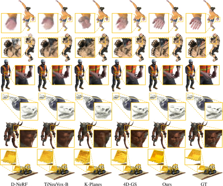
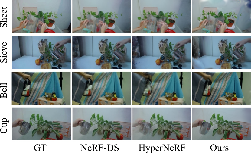
We also conduct qualitative comparisons to illustrate the advantages of our method over SOTA methods. The comparisons on D-NeRF datasets are shown in Fig. 3, where zoom-in images show the details of synthesized images. Our approach produces results closest to the ground truths and has the best visual quality. Note that, in the Lego scene, the motion in the test set does not align with that in the training set, as indicated in the bottom row of the figure. The same observation can also be seen in [47]. The qualitative comparisons conducted on the NeRF-DS dataset are also demonstrated in Fig. 4. It is clear that our method is capable of producing high-fidelity novel views, even in the absence of a specialized design for specular surfaces.

Table 3: We quantitatively evaluate the effect of control points and ARAP loss on D-NeRF [30] datasets.

Methods	PSNR($\uparrow$)	SSIM($\uparrow$)	LPIPS($\downarrow$)
w/o Control Points	38.512	0.9922	0.0162
w/o ARAP loss	42.617	0.9963	0.0067
Full	43.307	0.9976	0.0063

6.4 Ablation study

Control Points. Our motion representation driven by control points constructs a compact and sparse motion space, effectively mitigating overfitting on the training set. We quantitatively compare the novel view synthesis quality of our method with the baseline that does not utilize control points on both D-NeRF [30] and NeRF-DS [46] datasets, as presented in Tab. 1 and Tab. 2. To intuitively elucidate the effects of control points, we compare the results and visualize the trajectories of Gaussians driven either with or without control points in Fig. 6 (a) and (b). Clearly, directly predicting the motion of each Gaussian with an MLP leads to noise in Gaussian trajectories. While the baseline theoretically is more flexible in representing diverse motions, it tends to falter and descend into local minima during optimization, hindering it from achieving the global optimum.

ARAP Loss. Despite the control-point-driven motion representation providing effective regularization to Gaussian motions, there can be occasional breaches in rigidity. As evidenced in Fig. 6 (c), even though Gaussians achieve relatively smooth trajectories, some Gaussians on the arm move towards the girl’s torso instead of moving alongside the ascending arm. This issue arises due to the lack of constraints on the inter-relation of control points’ motions. By imposing ARAP loss on control points, such phenomena are eliminated, thus facilitating a robust motion reconstruction. Tab. 3 illustrates without ARAP loss, the performance of dynamic view synthesis on D-NeRF [30] slightly decreases.

Figure 6: We visualize the rendering results and Gaussian trajectories of (a) the baseline method without control points, (b) our full method, and (c) our method without ARAP loss.

6.5 Motion Editing

Our method facilitates scene motion editing via the manipulation of control nodes, due to the explicit motion representation using control points. The learned correlation and weights between Gaussians and control points enable excellent generalization, even on motion beyond the training sequence. The reconstructed and edited motion sequences are demonstrated in Fig. 5.

7 Conclusion and Limitations

We present a method driving 3D Gaussians using control points and a deformation MLP, learnable from dynamic scenes. Our approach, combining a compact motion representation with adaptive learning strategies and rigid constraints, allows high-quality dynamic scene reconstruction and motion editing. Experiments showed our method outperforms existing approaches in the visual quality of synthesized dynamic novel views. However, limitations exist. The performance is prone to inaccurate camera poses, leading to reconstruction failures on datasets with inaccurate poses such as HyperNeRF [27]. The approach can also overfit datasets with sparse viewpoints or limited angle coverage. Finally, the method has been tested only in scenes with modest motion changes. Extending its applicability to intense movements remains an area of exploration.

References

- Barron et al. [2021] Jonathan T Barron, Ben Mildenhall, Matthew Tancik, Peter Hedman, Ricardo Martin-Brualla, and Pratul P Srinivasan. Mip-nerf: A multiscale representation for anti-aliasing neural radiance fields. In Proceedings of the IEEE/CVF International Conference on Computer Vision, pages 5855–5864, 2021.
- Barron et al. [2022] Jonathan T Barron, Ben Mildenhall, Dor Verbin, Pratul P Srinivasan, and Peter Hedman. Mip-nerf 360: Unbounded anti-aliased neural radiance fields. In Proceedings of the IEEE/CVF Conference on Computer Vision and Pattern Recognition, pages 5470–5479, 2022.
- Barron et al. [2023] Jonathan T Barron, Ben Mildenhall, Dor Verbin, Pratul P Srinivasan, and Peter Hedman. Zip-nerf: Anti-aliased grid-based neural radiance fields. arXiv preprint arXiv:2304.06706, 2023.
- Cao and Johnson [2023] Ang Cao and Justin Johnson. Hexplane: A fast representation for dynamic scenes. In 2023 IEEE/CVF Conference on Computer Vision and Pattern Recognition (CVPR), pages 130–141, 2023.
- Dou et al. [2016] Mingsong Dou, Sameh Khamis, Yury Degtyarev, Philip Davidson, Sean Ryan Fanello, Adarsh Kowdle, Sergio Orts Escolano, Christoph Rhemann, David Kim, Jonathan Taylor, et al. Fusion4d: Real-time performance capture of challenging scenes. ACM Transactions on Graphics (ToG), 35(4):1–13, 2016.
- Du et al. [2021] Yilun Du, Yinan Zhang, Hong-Xing Yu, Joshua B Tenenbaum, and Jiajun Wu. Neural radiance flow for 4d view synthesis and video processing. In 2021 IEEE/CVF International Conference on Computer Vision (ICCV), pages 14304–14314. IEEE Computer Society, 2021.
- Fang et al. [2022] Jiemin Fang, Taoran Yi, Xinggang Wang, Lingxi Xie, Xiaopeng Zhang, Wenyu Liu, Matthias Nießner, and Qi Tian. Fast dynamic radiance fields with time-aware neural voxels. In SIGGRAPH Asia 2022 Conference Papers, 2022.
- Fridovich-Keil et al. [2022] Sara Fridovich-Keil, Alex Yu, Matthew Tancik, Qinhong Chen, Benjamin Recht, and Angjoo Kanazawa. Plenoxels: Radiance fields without neural networks. In Proceedings of the IEEE/CVF Conference on Computer Vision and Pattern Recognition, pages 5501–5510, 2022.
- Gao et al. [2021] Chen Gao, Ayush Saraf, Johannes Kopf, and Jia-Bin Huang. Dynamic view synthesis from dynamic monocular video. In Proceedings of the IEEE/CVF International Conference on Computer Vision, pages 5712–5721, 2021.
- Gao and Tedrake [2019] Wei Gao and Russ Tedrake. Surfelwarp: Efficient non-volumetric single view dynamic reconstruction. arXiv preprint arXiv:1904.13073, 2019.
- Guo et al. [2023] Xiang Guo, Jiadai Sun, Yuchao Dai, Guanying Chen, Xiaoqing Ye, Xiao Tan, Errui Ding, Yumeng Zhang, and Jingdong Wang. Forward flow for novel view synthesis of dynamic scenes. In Proceedings of the IEEE/CVF International Conference on Computer Vision, pages 16022–16033, 2023.
- Kerbl et al. [2023] Bernhard Kerbl, Georgios Kopanas, Thomas Leimkühler, and George Drettakis. 3d gaussian splatting for real-time radiance field rendering. ACM Transactions on Graphics (ToG), 42(4):1–14, 2023.
- Li et al. [2009] Hao Li, Bart Adams, Leonidas J Guibas, and Mark Pauly. Robust single-view geometry and motion reconstruction. ACM Transactions on Graphics (ToG), 28(5):1–10, 2009.
- Li et al. [2022] Tianye Li, Mira Slavcheva, Michael Zollhoefer, Simon Green, Christoph Lassner, Changil Kim, Tanner Schmidt, Steven Lovegrove, Michael Goesele, Richard Newcombe, et al. Neural 3d video synthesis from multi-view video. In Proceedings of the IEEE/CVF Conference on Computer Vision and Pattern Recognition, pages 5521–5531, 2022.
- Li et al. [2021] Zhengqi Li, Simon Niklaus, Noah Snavely, and Oliver Wang. Neural scene flow fields for space-time view synthesis of dynamic scenes. In Proceedings of the IEEE/CVF Conference on Computer Vision and Pattern Recognition, pages 6498–6508, 2021.
- Li et al. [2023] Zhengqi Li, Qianqian Wang, Forrester Cole, Richard Tucker, and Noah Snavely. Dynibar: Neural dynamic image-based rendering. In Proceedings of the IEEE/CVF Conference on Computer Vision and Pattern Recognition, pages 4273–4284, 2023.
- Lin et al. [2022] Haotong Lin, Sida Peng, Zhen Xu, Yunzhi Yan, Qing Shuai, Hujun Bao, and Xiaowei Zhou. Efficient neural radiance fields for interactive free-viewpoint video. In SIGGRAPH Asia 2022 Conference Papers, pages 1–9, 2022.
- Lin et al. [2023] Haotong Lin, Sida Peng, Zhen Xu, Tao Xie, Xingyi He, Hujun Bao, and Xiaowei Zhou. Im4d: High-fidelity and real-time novel view synthesis for dynamic scenes. arXiv preprint arXiv:2310.08585, 2023.
- Lipman et al. [2005] Yaron Lipman, Olga Sorkine-Hornung, Marc Alexa, Daniel Cohen-Or, David Levin, Christian Rössl, and Hans-Peter Seidel. Laplacian framework for interactive mesh editing. Int. J. Shape Model., 11:43–62, 2005.
- Liu et al. [2022] Jia-Wei Liu, Yan-Pei Cao, Weijia Mao, Wenqiao Zhang, David Junhao Zhang, Jussi Keppo, Ying Shan, Xiaohu Qie, and Mike Zheng Shou. Devrf: Fast deformable voxel radiance fields for dynamic scenes. Advances in Neural Information Processing Systems, 35:36762–36775, 2022.
- Lombardi et al. [2021] Stephen Lombardi, Tomas Simon, Gabriel Schwartz, Michael Zollhoefer, Yaser Sheikh, and Jason Saragih. Mixture of volumetric primitives for efficient neural rendering. ACM Transactions on Graphics (ToG), 40(4):1–13, 2021.
- Luiten et al. [2024] Jonathon Luiten, Georgios Kopanas, Bastian Leibe, and Deva Ramanan. Dynamic 3d gaussians: Tracking by persistent dynamic view synthesis. In 3DV, 2024.
- Mildenhall et al. [2021] Ben Mildenhall, Pratul P Srinivasan, Matthew Tancik, Jonathan T Barron, Ravi Ramamoorthi, and Ren Ng. Nerf: Representing scenes as neural radiance fields for view synthesis. Communications of the ACM, 65(1):99–106, 2021.
- Müller et al. [2022] Thomas Müller, Alex Evans, Christoph Schied, and Alexander Keller. Instant neural graphics primitives with a multiresolution hash encoding. ACM Transactions on Graphics (ToG), 41(4):1–15, 2022.
- Newcombe et al. [2015] Richard A Newcombe, Dieter Fox, and Steven M Seitz. Dynamicfusion: Reconstruction and tracking of non-rigid scenes in real-time. In Proceedings of the IEEE conference on computer vision and pattern recognition, pages 343–352, 2015.
- Park et al. [2021a] Keunhong Park, Utkarsh Sinha, Jonathan T Barron, Sofien Bouaziz, Dan B Goldman, Steven M Seitz, and Ricardo Martin-Brualla. Nerfies: Deformable neural radiance fields. In Proceedings of the IEEE/CVF International Conference on Computer Vision, pages 5865–5874, 2021a.
- Park et al. [2021b] Keunhong Park, Utkarsh Sinha, Peter Hedman, Jonathan T. Barron, Sofien Bouaziz, Dan B Goldman, Ricardo Martin-Brualla, and Steven M. Seitz. Hypernerf: A higher-dimensional representation for topologically varying neural radiance fields. ACM, 2021b.
- Park et al. [2023] Sungheon Park, Minjung Son, Seokhwan Jang, Young Chun Ahn, Ji-Yeon Kim, and Nahyup Kang. Temporal interpolation is all you need for dynamic neural radiance fields. In Proceedings of the IEEE/CVF Conference on Computer Vision and Pattern Recognition, pages 4212–4221, 2023.
- Peng et al. [2023] Sida Peng, Yunzhi Yan, Qing Shuai, Hujun Bao, and Xiaowei Zhou. Representing volumetric videos as dynamic mlp maps. In Proceedings of the IEEE/CVF Conference on Computer Vision and Pattern Recognition, pages 4252–4262, 2023.
- Pumarola et al. [2021] Albert Pumarola, Enric Corona, Gerard Pons-Moll, and Francesc Moreno-Noguer. D-nerf: Neural radiance fields for dynamic scenes. In Proceedings of the IEEE/CVF Conference on Computer Vision and Pattern Recognition, pages 10318–10327, 2021.
- Sara Fridovich-Keil and Giacomo Meanti et al. [2023] Sara Fridovich-Keil and Giacomo Meanti, Frederik Rahbæk Warburg, Benjamin Recht, and Angjoo Kanazawa. K-planes: Explicit radiance fields in space, time, and appearance. In CVPR, 2023.
- Schönberger and Frahm [2016] Johannes Lutz Schönberger and Jan-Michael Frahm. Structure-from-motion revisited. In Conference on Computer Vision and Pattern Recognition (CVPR), 2016.
- Shao et al. [2023] Ruizhi Shao, Zerong Zheng, Hanzhang Tu, Boning Liu, Hongwen Zhang, and Yebin Liu. Tensor4d: Efficient neural 4d decomposition for high-fidelity dynamic reconstruction and rendering. In Proceedings of the IEEE Conference on Computer Vision and Pattern Recognition, 2023.
- Sorkine and Alexa [2007] Olga Sorkine and Marc Alexa. As-rigid-as-possible surface modeling. In Symposium on Geometry processing, pages 109–116. Citeseer, 2007.
- Sorkine-Hornung [2005] Olga Sorkine-Hornung. Laplacian mesh processing. In Eurographics, 2005.
- Sorkine-Hornung et al. [2004] Olga Sorkine-Hornung, Daniel Cohen-Or, Yaron Lipman, Marc Alexa, Christian Rössl, and Hans-Peter Seidel. Laplacian surface editing. In Eurographics Symposium on Geometry Processing, 2004.
- Sumner et al. [2007] Robert W Sumner, Johannes Schmid, and Mark Pauly. Embedded deformation for shape manipulation. In ACM siggraph 2007 papers, pages 80–es. 2007.
- Tretschk et al. [2021] Edgar Tretschk, Ayush Tewari, Vladislav Golyanik, Michael Zollhöfer, Christoph Lassner, and Christian Theobalt. Non-rigid neural radiance fields: Reconstruction and novel view synthesis of a dynamic scene from monocular video. In Proceedings of the IEEE/CVF International Conference on Computer Vision, pages 12959–12970, 2021.
- Wang et al. [2023a] Feng Wang, Sinan Tan, Xinghang Li, Zeyue Tian, Yafei Song, and Huaping Liu. Mixed neural voxels for fast multi-view video synthesis. In Proceedings of the IEEE/CVF International Conference on Computer Vision, pages 19706–19716, 2023a.
- Wang et al. [2023b] Liao Wang, Qiang Hu, Qihan He, Ziyu Wang, Jingyi Yu, Tinne Tuytelaars, Lan Xu, and Minye Wu. Neural residual radiance fields for streamably free-viewpoint videos. In Proceedings of the IEEE/CVF Conference on Computer Vision and Pattern Recognition, pages 76–87, 2023b.
- Wang et al. [2021] Peng Wang, Lingjie Liu, Yuan Liu, Christian Theobalt, Taku Komura, and Wenping Wang. Neus: Learning neural implicit surfaces by volume rendering for multi-view reconstruction. arXiv preprint arXiv:2106.10689, 2021.
- Wu et al. [2023] Guanjun Wu, Taoran Yi, Jiemin Fang, Lingxi Xie, Xiaopeng Zhang, Wei Wei, Wenyu Liu, Qi Tian, and Wang Xinggang. 4d gaussian splatting for real-time dynamic scene rendering. arXiv preprint arXiv:2310.08528, 2023.
- Xian et al. [2021] Wenqi Xian, Jia-Bin Huang, Johannes Kopf, and Changil Kim. Space-time neural irradiance fields for free-viewpoint video. In Proceedings of the IEEE/CVF Conference on Computer Vision and Pattern Recognition, pages 9421–9431, 2021.
- Xu and Harada [2022] Tianhan Xu and Tatsuya Harada. Deforming radiance fields with cages. In ECCV, 2022.
- Xu et al. [2023] Zhen Xu, Sida Peng, Haotong Lin, Guangzhao He, Jiaming Sun, Yujun Shen, Hujun Bao, and Xiaowei Zhou. 4k4d: Real-time 4d view synthesis at 4k resolution. arXiv preprint arXiv:2310.11448, 2023.
- Yan et al. [2023] Zhiwen Yan, Chen Li, and Gim Hee Lee. Nerf-ds: Neural radiance fields for dynamic specular objects. In Proceedings of the IEEE/CVF Conference on Computer Vision and Pattern Recognition, pages 8285–8295, 2023.
- Yang et al. [2023a] Ziyi Yang, Xinyu Gao, Wen Zhou, Shaohui Jiao, Yuqing Zhang, and Xiaogang Jin. Deformable 3d gaussians for high-fidelity monocular dynamic scene reconstruction. arXiv preprint arXiv:2309.13101, 2023a.
- Yang et al. [2023b] Zeyu Yang, Hongye Yang, Zijie Pan, Xiatian Zhu, and Li Zhang. Real-time photorealistic dynamic scene representation and rendering with 4d gaussian splatting. arXiv preprint arXiv 2310.10642, 2023b.
- Yifan et al. [2020] Wang Yifan, Noam Aigerman, Vladimir G. Kim, Siddhartha Chaudhuri, and Olga Sorkine-Hornung. Neural cages for detail-preserving 3D deformations. In Proceedings of the IEEE/CVF Conference on Computer Vision and Pattern Recognition, pages 75–83, 2020.
- Yu et al. [2021] Alex Yu, Ruilong Li, Matthew Tancik, Hao Li, Ren Ng, and Angjoo Kanazawa. Plenoctrees for real-time rendering of neural radiance fields. In Proceedings of the IEEE/CVF International Conference on Computer Vision, pages 5752–5761, 2021.
- Yu et al. [2004] Yizhou Yu, Kun Zhou, Dong Xu, Xiaohan Shi, Hujun Bao, Baining Guo, and Heung-Yeung Shum. Mesh editing with Poisson-based gradient field manipulation. In ACM SIGGRAPH 2004 Papers, pages 644–651. 2004.
- Yuan et al. [2022] Yu-Jie Yuan, Yang-Tian Sun, Yu-Kun Lai, Yuewen Ma, Rongfei Jia, and Lin Gao. Nerf-editing: Geometry editing of neural radiance fields. 2022 IEEE/CVF Conference on Computer Vision and Pattern Recognition (CVPR), pages 18332–18343, 2022.
- Zhang et al. [2018] Richard Zhang, Phillip Isola, Alexei A. Efros, Eli Shechtman, and Oliver Wang. The unreasonable effectiveness of deep features as a perceptual metric. pages 586–595, 2018.
- Zhang et al. [2020] Yuzhe Zhang, Jianmin Zheng, and Yiyu Cai. Proxy-driven free-form deformation by topology-adjustable control lattice. Computers & Graphics, 89:167–177, 2020.