Resurgence of refined topological strings and dual partition functions

Abstract

We study the resurgent structure of the refined topological string partition function on a non-compact Calabi-Yau threefold, at large orders in the string coupling constant $g_{s}$ and fixed refinement parameter ${\mathsf{b}}$. For ${\mathsf{b}}\neq 1$, the Borel transform admits two families of simple poles, corresponding to integral periods rescaled by ${\mathsf{b}}$ and $1/{\mathsf{b}}$. We show that the corresponding Stokes automorphism is expressed in terms of a generalization of the non-compact quantum dilogarithm, and we conjecture that the Stokes constants are determined by the refined DT invariants counting spin-$j$ BPS states. This jump in the refined topological string partition function is a special case (unit five-brane charge) of a more general transformation property of wave functions on quantum twisted tori introduced in earlier work by two of the authors. We show that this property follows from the transformation of a suitable refined dual partition function across BPS rays, defined by extending the Moyal star product to the realm of contact geometry.

1 Introduction

As a mathematically well-defined subsector of type II superstring theories, topological string theory provides a prime arena for exploring the non-perturbative completion of the asymptotic series predicted by the perturbative genus expansion in string theory. In cases where the target Calabi-Yau threefold $X$ admits a large $N$ dual, a non-perturbative formulation is available, which resums the perturbative series to all orders in the topological string coupling $g_{s}=1/N$, for fixed values of the moduli $\boldsymbol{t}$ (corresponding to t’Hooft couplings in the dual gauge theory) at least for integer values of $N$. Non-perturbative corrections of order $e^{-1/g_{s}}$ typically arise from tunneling (or instanton) effects in the dual matrix model. In general however, one has only access to the genus-$g$ free energy ${\cal F}_{g}(\boldsymbol{t})$ occurring at order $g_{s}^{2g-2}$ in the perturbative expansion, and non-perturbative corrections are ambiguous, without further assumptions.

Assuming that the putative, non-perturbative topological string partition function ${\cal F}(\boldsymbol{t};g_{s})$ belongs to a suitable class of resurgent functions, one can however extract much information about non-perturbative corrections from the growth of the coefficients ${\cal F}_{g}(\boldsymbol{t})$ at large genus. This method was proposed early on in Shenker:1990uf for general string theory models, and first applied to the topological string in mm-open ; msw ; mmnp ; ps09 . In particular, the instanton action ${\cal A}$ controlling the size of the leading instanton effects $e^{-{\cal A}/g_{s}}$ can be read off from the location of the singularity closest to the origin in the Borel plane.

While the explicit computation of the free energies ${\cal F}_{g}(\boldsymbol{t})$ is usually impractical at large genus, they are strongly constrained by the holomorphic anomaly equations (HAE) bcov . Following cesv1 ; cesv2 , much progress has been made recently in constructing the trans-series solution to the HAE gm-multi ; gkkm ; Iwaki:2023cek ; ms . In particular, it was shown that the instanton actions ${\cal A}$ entering in the trans-series are equal (up to overall normalization) to the central charge $Z(\gamma)$ of vectors $\gamma$ in the charge lattice (the Grothendieck lattice $K_{0}(X)$ in the $A$-model, or the homology lattice $H_{3}(X,{\mathbb{Z}})$ in the B-model). Moreover, the Stokes automorphism $\mathfrak{S}$ controlling the jump in the Borel resummation when a radial integration contour crosses a sequence of singularities was determined in Iwaki:2023cek : the jump induces the following transformation in the partition function ${\cal Z}=e^{{\cal F}}$,

$${\cal Z}\ \mapsto\ \mathfrak{S}{\cal Z}=\exp\left[\frac{\omega(\gamma)}{2\pi{\rm i}}\left({\rm Li}_{2}(e^{2\pi x})+2\pi x\log(1-e^{2\pi x})\right)\right]{\cal Z},$$ (1.1)

where $\omega(\gamma)$ is (up to normalization) the so-called Stokes constant, ${\rm Li}_{2}(z)=\sum_{k\geq 1}z^{k}/k^{2}$ is the dilogarithm function and $x$ is suitable operator (equal to $\frac{{\rm i}g_{s}}{2\pi}c^{a}\partial_{t^{a}}$ in the simplest case considered in Iwaki:2023cek , which we also restrict to here for simplicity; here $c^{a}$ are the components of $\gamma$ in $H_{4}(X,{\mathbb{Z}})$, interpreted as D4-brane charges in type IIA set-up, or D3-brane charges in type IIB). As observed in Iwaki:2023cek , the transformation (1.1) is exactly such that the so-called dual partition function

$$\tau(\boldsymbol{t},\boldsymbol{u};g_{s})=\sum_{\boldsymbol{n}\in{\mathbb{Z}}^{n}}e^{2\pi\boldsymbol{n}\cdot\boldsymbol{u}/g_{s}}\,{\cal Z}(\boldsymbol{t}-{\rm i}g_{s}\boldsymbol{n};g_{s})$$ (1.2)

transforms by a simple factor, up to a $\boldsymbol{u}$-dependent shift in $\boldsymbol{t}$,

$$\mathfrak{S}\tau(\boldsymbol{t},\boldsymbol{u};g_{s})=e^{\frac{\omega(\gamma)}{2\pi{\rm i}}\,{\rm Li}_{2}({\rm e}^{2\pi{\boldsymbol{c}}\cdot\boldsymbol{u}/g_{s}})}\,\tau\left(\boldsymbol{t}+\frac{\omega(\gamma)}{2\pi}\,g_{s}{\boldsymbol{c}}\,\log\left(1-{\rm e}^{2\pi{\boldsymbol{c}}\cdot\boldsymbol{u}/g_{s}}\right),\boldsymbol{u};g_{s}\right).$$ (1.3)

We note that dual partition functions (which are obtained as so-called Zak transforms of the conventional partition functions) have appeared in many different contexts, including supersymmetric gauge theories no2 , topological string theory adkmv ; dhsv , topological recursion em ; Eynard:2021sxg , the spectral theory/topological string correspondence ghm and isomonodromic tau functions GIL-12 ; GIL-13 ; cpt ; CLT .

Quite remarkably, the transformations (1.1) and (1.3) have appeared before in yet a different context, namely the study of five-brane instanton corrections to the hypermultiplet moduli space in type II strings compactified on a Calabi-Yau threefold APP ; Alexandrov:2015xir . The key idea of APP ; Alexandrov:2015xir is that S-duality relates NS5-brane instanton corrections in type IIB string theory to D5-brane instanton corrections, which (for unit D5-brane charge) are governed by the topological string partition function by virtue of gw-dt ; gw-dt2 . More specifically, for fixed unit D5-brane charge, the sum over D3-D1-D(-1) brane charges leads to a non-Gaussian theta series of the form (1.2) (with $\boldsymbol{n}$ being the D3-brane charge). Due to wall-crossing behavior of the Donaldson-Thomas (DT) invariants $\Omega(\gamma)$ counting D5-D3-D1-D(-1) instantons in type IIB (or equivalently D6-D4-D2-D0 black holes in type IIA), the theta series becomes a section of a certain line bundle ${\cal L}$ over the (twistor space of) the hypermultiplet moduli space, with gluing conditions given by (1.3), which in turn imply the transformation (1.1) for the kernel of the theta series. This suggests in particular that the Stokes constant $\omega(\gamma)$ should be equated with the DT invariant $\Omega(\gamma)$ counting BPS states associated to the same ray, as proposed in different contexts in mm-s2019 ; gm-peacock ; astt ; gm-multi ; gkkm ; gu-res . These considerations were extended in Alexandrov:2015xir in two directions: first, to $k>1$ units of five-brane charge, where the theta series becomes a section of the $k$-th power of the line bundle ${\cal L}$, and second, to include the effect of the refinement parameter $y$ in Donaldson-Thomas theory, conjugate to angular momentum, which induces a non-commutative deformation of the (twistor space of the) hypermultiplet moduli space.

This brings us to the main goal of the present paper, which is to extend the results (1.1)–(1.3) to the refined topological string partition function. The latter can be viewed as a one-parameter deformation ${\cal F}(\boldsymbol{t};g_{s},{\mathsf{b}})$ of the usual topological free energy ${\cal F}(\boldsymbol{t};g_{s})$, which exists on non-compact Calabi-Yau threefolds with a ${\mathbb{C}}^{\times}$ action. While the worldsheet definition of refined topological strings for ${\mathsf{b}}\neq 1$ remains obscure (see Antoniadis:2013bja for an early attempt), in space-time it is interpreted as the partition function of the five-dimensional gauge theory engineered by M-theory compactified on $X$ times a five-dimensional $\Omega$-background n ; Nekrasov:2010ka with parameters

$$\epsilon_{1}=g_{s}{\mathsf{b}},\qquad\epsilon_{2}=-g_{s}{\mathsf{b}}^{-1}.$$ (1.4)

The resulting partition function leads to integer BPS invariants $N_{\boldsymbol{d}}^{j_{L},j_{R}}$ which refine the usual Gopakumar–Vafa and Donaldson-Thomas invariants hiv ; ckk ; no . When $X$ is a toric CY singularity, ${\cal F}(\boldsymbol{t};g_{s},{\mathsf{b}})$ can be computed by a refined version ikv of the topological vertex formalism akmv . Otherwise, the main computational tool is the refined version hk of the standard holomorphic anomaly equations (HAE) bcov , which can be integrated inductively with sufficient control on the behavior at boundaries of moduli space.

In this work, we extend the analysis of gm-multi ; Iwaki:2023cek and construct the general trans-series solution to the refined HAE. In particular, we find that there are now two instanton actions ${\mathsf{b}}Z(\gamma)$ and ${\mathsf{b}}^{-1}Z(\gamma)$ contributing to the trans-series for each $\gamma$ in the charge lattice. Moreover, in the simplest case where the singularity corresponds to a BPS state with unit Stokes constant $\omega(\gamma)=1$ (as befits states which become massless at a conifold singularity), we find that the Stokes automorphism (1.1) is deformed to

$$\mathfrak{S}_{{\mathsf{b}}}{\cal Z}=\Phi_{{\mathsf{b}}}^{-1}(x)\,{\cal Z},$$ (1.5)

where $\Phi_{{\mathsf{b}}}(x)$ is the Faddeev quantum dilogarithm defined in (A.132), reducing to (1.1) at ${\mathsf{b}}=1$ due to (A.135). More generally, the Stokes automorphism associated to a singularity supported at $Z(\gamma)$ is given by

$$\mathfrak{S}_{{\mathsf{b}}}{\cal Z}=\prod_{j}\left[\prod_{m=-j}^{j}\Phi_{\mathsf{b}}\left(x+{\rm i}m({\mathsf{b}}-{\mathsf{b}}^{-1})\right)\right]^{-\omega_{[j]}}{\cal Z},$$ (1.6)

where the product runs over half integer $m$ such that $m+j$ is integer, and $\omega_{[j]}$ are Stokes constants. This has a natural interpretation in terms of motivic or refined DT invariants, which can be decomposed as $\Omega(\gamma,y)=\sum_{j}\Omega_{[j]}(\gamma)\chi_{j}(y)$, where

$$\chi_{j}(y):=\sum_{m=-j}^{j}y^{2m}=\frac{y^{2j+1}-y^{-2j-1}}{y-y^{-1}}$$ (1.7)

is the character of the spin $j$ representation of $SU(2)$. We conjecture that the Stokes constants $\omega_{[j]}$ associated to the singularity at $Z(\gamma)$ are equal to the coefficients $\Omega_{[j]}(\gamma)$ appearing in this decomposition.

It is then natural to ask whether there exists a deformation of the dual partition function (1.2), with kernel given by the refined topological string partition function ${\cal Z}$, whose transformation rules across rays would be guaranteed by the Stokes automorphism (1.5), or more generally (1.6). In fact, the Stokes automorphism (1.5) is a special case $k=1$ of an operator ${\bf A}_{{\mathsf{b}}^{2}}^{(k)}$ acting on $L^{2}({\mathbb{R}})\otimes{\mathbb{C}}^{k}$ which was introduced in (Alexandrov:2015xir, , §4) in a rather ad hoc fashion, for the purpose of producing a doubly-quantized version of the standard 5-term relation for the quantum dilogarithm. In this work, we provide a rationale for the construction of (Alexandrov:2015xir, , §4), by explicitly constructing a generalized theta series valued in a degree $k$ line bundle ${\cal L}_{{\mathsf{b}}}$ over the quantum torus, which is well defined across BPS rays provided the kernel of the theta series transforms according to ${\bf A}_{{\mathsf{b}}^{2}}^{(k)}$, or more generally by a $j$-dependent extension of ${\bf A}_{{\mathsf{b}}^{2}}^{(k)}$. For $k=1$, this provides a refined version of the dual partition function (1.2). Both the theta series and its transformation under wall-crossing are defined using a certain Moyal-type non-commutative product on twistor space. In fact, the non-commutativity makes it possible to introduce two different refined dual partition functions which are both related to the refined topological string partition function, but with one of the twistor space coordinates identified with (the inverse of) either of the two deformation parameters $\epsilon_{1,2}$ from (1.4).

These results raise several obvious questions: first, can one prove the equality between Stokes constants and Donaldson-Thomas invariants, perhaps in the framework of the Riemann-Hilbert problem proposed in Bri-19 ; Barbieri:2019yya ; Bridgeland:2020zjh ; Alexandrov:2021wxu ; Bri-23 ? Second, what is the physical interpretation of the refined dual partition function, for example in terms of free fermions, spectral determinants, tau functions, partition functions of line defects, or otherwise? Third, does there exists a rank-$k$ version of the topological string (refined or unrefined) whose large order behavior would be governed by the Stokes automorphism ${\bf A}_{{\mathsf{b}}^{2}}^{(k)}$, and which would be related to the partition function of $k$ five-branes constructed in (Alexandrov:2010ca, , §5) by a rank-$k$ version of the GV/DT correspondence gw-dt ? We hope to return to some of these challenging problems in the near future.

The remainder of this work is organized as follows. In §2 we review basic properties of the refined topological string free energy. In §3 we construct the trans-series solution of the holomorphic anomaly equations, determine the boundary conditions at the conifold locus and in the large volume limit, deduce the Stokes automorphism associated to the singularities in the Borel plane, and perform numerical checks in the case of $X=K_{{\mathbb{P}}^{2}}$. In §4, we recover the same automorphism and generalize it to any integer $k\geq 1$ by constructing a class of dual partition functions on quantum twisted tori. Definitions and properties of several variants of the quantum dilogarithm function, which plays a central role in this work, are collected in Appendix §A.

Acknowledgements: The authors would like to thank Murad Alim, Tom Bridgeland, Alba Grassi, Jie Gu and Joerg Teschner for valuable discussions. The research of MM is supported in part by the ERC-SyG project “Recursive and Exact New Quantum Theory” (ReNewQuantum), which received funding from the European Research Council (ERC) under the European Union’s Horizon 2020 research and innovation program, grant agreement No. 810573. The research of BP is supported by Agence Nationale de la Recherche under contract number ANR-21-CE31-0021. SA and BP would like to thank the Isaac Newton Institute for Mathematical Sciences in Cambridge (supported by EPSRC grant EP/R014604/1), for hospitality during the programme Black holes: bridges between number theory and holographic quantum information where work on this project was undertaken.

2 The refined topological string

In this section, we review some basic facts about the refined topological string and how to calculate its free energy.

As mentioned above, the refined topological string is parametrized by two complex parameters $\epsilon_{1,2}$. Setting

$$\epsilon_{1}=g_{s}{\mathsf{b}},\qquad\epsilon_{2}=-g_{s}{\mathsf{b}}^{-1},$$ (2.1)

the parameter $g_{s}$ can be identified as the topological string coupling constant, while ${\mathsf{b}}$ can be regarded as a deformation parameter. When ${\mathsf{b}}=1$ one recovers the standard topological string. We note that many references (like kw ) use a parameter $\beta$, which is related to ours simply by ${\mathsf{b}}=\beta^{1/2}$. The refined topological string free energy is a formal power series hk

$${\cal F}({\boldsymbol{t}};\epsilon_{1},\epsilon_{2})=\sum_{i,j\geq 0}(\epsilon_{1}+\epsilon_{2})^{2i}\,(-\epsilon_{1}\epsilon_{2})^{j-1}{\cal F}^{(i,j)}(\boldsymbol{t}),$$ (2.2)

where the coefficients ${\cal F}^{(i,j)}(\boldsymbol{t})$ are sections of an appropriate line bundle on the moduli space of $X$ (of Kähler structures in the A-model, or complex structures in the B-model), parametrized by the flat coordinates ${\boldsymbol{t}}$. For the purposes of this paper, we regard the free energy as a formal power series in $g_{s}$ whose coefficients depend on the moduli and on the deformation parameter ${\mathsf{b}}$,

$${\cal F}({\boldsymbol{t}};g_{s},{\mathsf{b}})=\sum_{g\geq 0}g_{s}^{2g-2}\,{\cal F}_{g}({\boldsymbol{t}};{\mathsf{b}}),$$ (2.3)

where

$${\cal F}_{g}({\boldsymbol{t}};{\mathsf{b}})=\sum_{k=0}^{g}{\cal F}^{(k,g-k)}({\boldsymbol{t}})\,({\mathsf{b}}-{\mathsf{b}}^{-1})^{2k}.$$ (2.4)

The deformed free energies ${\cal F}_{g}({\boldsymbol{t}};{\mathsf{b}})$ are Laurent polynomials in ${\mathsf{b}}$, of degree $2g$, and invariant under the exchange ${\mathsf{b}}\leftrightarrow{\mathsf{b}}^{-1}$. When ${\mathsf{b}}=1$,

$${\cal F}_{g}({\boldsymbol{t}};1)={\cal F}^{(0,g)}({\boldsymbol{t}})={\cal F}_{g}({\boldsymbol{t}})$$ (2.5)

is the conventional, unrefined topological string free energy at genus $g$. The amplitudes ${\cal F}^{(k,g-k)}({\boldsymbol{t}})$ are related to the ones defined in hk by an overall sign $(-1)^{k}$.

The refined free energies ${\cal F}_{g}({\boldsymbol{t}};{\mathsf{b}})$ can be calculated on certain local CY geometries using instanton calculus n , and more generally with the refined topological vertex of ikv . These A-model-like calculations are intrinsically attached to the large radius of the geometry. In the refined case, the B-model approach to the free energies is based on the HAE of bcov . An extension of the HAE to the refined case was proposed in hk (see also kw ), and tested in detail in e.g. hkk ; ckk . In the framework of the HAE, one extends the free energies ${\cal F}_{g}({\boldsymbol{t}};{\mathsf{b}})$ to non-holomorphic functions, and the HAE control their non-holomorphic dependence. We will use Roman capital letters for the non-holomorphic free energies obtained from the HAE, and curly capital letters for their holomorphic limit, as in gm-multi ; gkkm .

To write the HAE, we need some ingredients from special geometry (see e.g. klemm for more details). In the local case, the mirror CY is encoded in an algebraic curve usually called the mirror curve. We recall that the moduli space ${\cal M}$ of complex structures of the mirror CY is a special Kähler manifold of complex dimension $n$. We will denote by $z^{a}$, with $a=1,\cdots,n$ a set of algebraic complex coordinates on this moduli space. The Kähler metric (here $\partial_{a}=\partial_{z^{a}}$)

$$G_{a\bar{b}}=\partial_{a}\partial_{\bar{b}}K$$ (2.6)

derives from a Kähler potential $K$, which is determined from the prepotential ${\cal F}_{0}$, equal to the genus zero free energy (the latter does not depend on ${\mathsf{b}}$, as it clear from (2.4)). We introduce the covariant derivative $D_{a}$ for the Levi–Civita connection associated to the metric,

$$\Gamma^{a}_{bc}=G^{a\bar{k}}\partial_{b}G_{c\bar{k}}.$$ (2.7)

In the case of compact CY threefolds, the covariant derivative involves as well a connection on the Hodge bundle ${\cal L}$ over ${\cal M}$, but since this connection vanishes in the holomorphic limit bcov we can take it to be zero from the very beginning, as noted in kz . The Yukawa couplings are determined from the genus 0 free energy via

$$C_{abc}=\partial_{a}\partial_{b}\partial_{c}{\cal F}_{0}.$$ (2.8)

Finally, we have to introduce an anti-holomorphic version of the Yukawa coupling, defined by

$${\overline{C}}_{\bar{c}}^{ab}={\rm e}^{2K}\,G^{a\bar{d}}G^{b\bar{e}}{\overline{C}}_{\bar{a}\bar{d}\bar{e}}.$$ (2.9)

We can now write the refined HAE, following hk . In terms of the free energies $F^{(k,g-k)}$, they read

$$\partial_{\bar{c}}F^{(k,g-k)}={1\over 2}\,\overline{C}^{ab}_{\bar{c}}\left(D_{a}D_{b}F^{(k,g-k-1)}+\sum_{m,h}D_{a}F^{(m,h)}D_{b}F^{(k-m,g-k-h)}\right),$$ (2.10)

where $g\geq 2$ and the sum over $m,h$ is such that $m+h\geq 1$. However, it is easy to check that, in terms of the combinations $F_{g}({\mathsf{b}})$ defined in (2.4), the HAE take the same form as in the unrefined case of bcov :

$$\partial_{\bar{c}}F_{g}({\mathsf{b}})={1\over 2}\,\overline{C}^{ab}_{\bar{c}}\left(D_{a}D_{b}F_{g-1}({\mathsf{b}})+\sum_{h=1}^{g-1}D_{a}F_{h}({\mathsf{b}})D_{b}F_{g-h}({\mathsf{b}})\right),\qquad g\geq 2.$$ (2.11)

(Here, we only indicate the dependence of the refined free energies on the deformation parameter, but they of course also depend on $z^{a}$.) Therefore, the refined free energies satisfy the same HAE as the unrefined ones, but the starting point of the recursion, given by the free energies at $g=1$, is different and given by

$$F_{1}({\mathsf{b}})=F_{1}({\mathsf{b}}=1)+({\mathsf{b}}-{\mathsf{b}}^{-1})^{2}F^{(1,0)}.$$ (2.12)

Here, $F_{1}({\mathsf{b}}=1)=F^{(0,1)}$ is the conventional, unrefined free energy at genus one. The free energy $F^{(1,0)}$ turns out to be given by a holomorphic function of the moduli. It has the form hk ; hkk

$$F^{(1,0)}=-{1\over 24}\log\left(f(\boldsymbol{z})\Delta(\boldsymbol{z})\right),$$ (2.13)

where $\Delta(\boldsymbol{z})$ is the discriminant of the mirror curve, and $f(\boldsymbol{z})$ is a rational function of the moduli, explicitly known in many cases. The fact that $F^{(1,0)}$ is holomorphic will be important later on.

As in the unrefined local case, it is useful to introduce propagators $S^{ab}$, defined by the condition that bcov

$$\partial_{\bar{c}}S^{ab}=\overline{C}^{ab}_{\bar{c}}.$$ (2.14)

The propagators contain the full anti-holomorphic dependence of the free energies. As a result, the HAE (2.11) can be rewritten in the form

$${\partial F_{g}({\mathsf{b}})\over\partial S^{ab}}={1\over 2}\left(D_{a}D_{b}F_{g-1}({\mathsf{b}})+\sum_{h=1}^{g-1}D_{a}F_{h}({\mathsf{b}})D_{b}F_{g-h}({\mathsf{b}})\right),\qquad g\geq 2.$$ (2.15)

The initial condition (2.12) has to be also re-expressed in terms of propagators. Since $F^{(1,0)}$ is purely holomorphic, it does not depend on the propagators, whereas for $F^{(0,1)}$ one has bcov

$$\partial_{a}F^{(0,1)}={1\over 2}\,C_{abc}S^{bc}+f_{a}(\boldsymbol{z}).$$ (2.16)

In this equation, $f_{a}(\boldsymbol{z})$ is a function of the moduli only. The equation (2.15), together with the initial conditions (2.12), (2.16) and (2.13), provides a recursive procedure to obtain the free energies $F_{g}({\mathsf{b}})$ as polynomials in the propagators, which is sometimes called “direct integration” yy ; hk06 ; gkmw . At each genus $g$ one has to fix an integration constant, independent of the propagators, but dependent on the moduli, and called the holomorphic ambiguity (the functions $f_{a}(\boldsymbol{z})$ in (2.16) can be regarded as examples thereof). In the case of local CY manifolds this ambiguity can be fixed in many cases by using the behavior of the free energies at special points in moduli space hkr . Let us review this behavior in the case of the refined topological string.

We first consider the behavior at the conifold locus, defined by the vanishing of a flat coordinate $t_{c}\to 0$. In the adapted symplectic frame, the free energy has the following behavior kw ; hk

$${\cal F}_{g}(t_{c};{\mathsf{b}})={c_{g}({\mathsf{b}})\over t_{c}^{2g-2}}+{\cal O}(1),$$ (2.17)

where the coefficient $c_{g}({\mathsf{b}})$ is given by

$$c_{g}({\mathsf{b}})=-(2g-3)!\sum_{m=0}^{g}\widehat{B}_{2m}\widehat{B}_{2g-2m}{\mathsf{b}}^{2(2m-g)},$$ (2.18)

where

$$\widehat{B}_{m}=(2^{1-m}-1)\,{B_{m}\over m!}$$ (2.19)

and $B_{m}$ is the Bernoulli number. In the unrefined limit ${\mathsf{b}}=1$ one has

$$c_{g}(1)={B_{2g}\over 2g(2g-2)},\qquad g\geq 2,$$ (2.20)

and one recovers the well-known universal conifold behavior of the standard topological string gv-conifold .

Another universal result concerns the behavior of the refined free energies at large radius. It is possible to generalize the Gopakumar–Vafa integrality structure gv to a refined version hiv ; hk . Let us introduce

$$\epsilon_{L,R}={\epsilon_{1}\mp\epsilon_{2}\over 2}\,.$$ (2.21)

In terms of the characters $\chi_{j}(y)$ defined in (1.7), the total free energy is then given, up to a cubic polynomial in $\boldsymbol{t}$, by a sum of the form

$${\cal F}({\boldsymbol{t}};g_{s},{\mathsf{b}})=\sum_{w,\boldsymbol{d}}\sum_{j_{L},j_{R}}\frac{\chi_{j_{L}}\left(e^{{\rm i}w\epsilon_{L}}\right)\chi_{j_{R}}\left(e^{{\rm i}w\epsilon_{R}}\right)}{4\sin\left({g_{s}w{\mathsf{b}}\over 2}\right)\sin\left({g_{s}w\over 2{\mathsf{b}}}\right)}\,N^{j_{L},j_{R}}_{\boldsymbol{d}}\,Q_{\boldsymbol{d}}^{w}\,,$$ (2.22)

where $Q_{\boldsymbol{d}}={\rm e}^{-\boldsymbol{d}\cdot\boldsymbol{c}}$ and $N^{j_{L},j_{R}}_{\boldsymbol{d}}$ are integers (here, $j_{L},j_{R}\in{\mathbb{Z}}^{+}/2$). The integers $N^{j_{L},j_{R}}_{\boldsymbol{d}}$ count BPS states with charge ${\boldsymbol{d}}$ transforming with spin $(j_{L},j_{R})$ under the little group $SU(2)_{L}\times SU(2)_{R}$ in 5 dimensions, and are sometimes called BPS invariants. When ${\mathsf{b}}=1$, we recover the integrality structure of the standard topological string free energy. In particular, we have the following relation between the genus zero Gopakumar–Vafa invariants $n^{(0)}_{\boldsymbol{d}}$ and the BPS invariants

$$n_{\boldsymbol{d}}^{(0)}=\sum_{j_{L},j_{R}}d_{L}d_{R}N^{j_{L},j_{R}}_{\boldsymbol{d}},\qquad d_{L,R}=2j_{L,R}+1.$$ (2.23)

The refined (or motivic) Donaldson-Thomas invariants $\Omega({\boldsymbol{d}},y)$ in the large volume limit are characters for the diagonal $SU(2)$ action:

$$\Omega({\boldsymbol{d}},y)=\sum_{j_{L},j_{R}}\chi_{j_{L}}(y)\,\chi_{j_{R}}(y)\,N^{j_{L},j_{R}}_{\boldsymbol{d}}.$$ (2.24)

In particular, they reduce to (2.23) in the unrefined limit $y\to 1$. Unlike the BPS invariants $N^{j_{L},j_{R}}_{\boldsymbol{d}}$, which are only defined when ${\boldsymbol{d}}$ is a curve class, the refined DT invariants $\Omega(\gamma,y)$ are defined for any vector $\gamma\in K_{0}(X)$, i.e. for arbitrary D6-D4-D2-D0 brane charge in type IIA, or D5-D3-D1-D(-1) charge in type IIB. For later purposes, it will be convenient to decompose $\Omega(\gamma,y)$ as a sum of $SU(2)$ characters,

$$\Omega(\gamma,y):=\sum_{j}\chi_{j}(y)\,\Omega_{[j]}(\gamma),$$ (2.25)

where the integers $\Omega_{[j]}(\gamma)$ count BPS multiplets of angular momentum $j\in{\mathbb{Z}}/2$, and $y$ is the corresponding fugacity parameter. We note that the representation (2.25) implies that $\Omega(\gamma,y)$ is a Laurent polynomial in $y$, invariant under Poincaré duality $y\mapsto 1/y$. As emphasized in Mozgovoy:2020has , for the standard definition of DT invariants using cohomology with compact supports, Poincaré duality is broken when $X$ is non-compact, primarily due to the non-invariance of the attractor indices counting D0-branes. Here we assume that the DT invariants which are pertinent for the refined topological string are in fact invariant under Poincaré duality.

3 Trans-series solutions and resurgent structure

In order to understand the resurgent structure of the refined topological string, we follow the strategy of cesv1 ; cesv2 ; cms ; gm-multi ; gkkm and look for trans-series solutions to the HAE. These define non-perturbative sectors of the theory, but they require boundary conditions, as in the perturbative case. As first pointed out in cesv1 ; cesv2 , we can obtain these boundary conditions by looking at the large order behavior of the genus expansions near special points in moduli space. It turns out that the first aspect of this procedure, namely the construction of formal trans-series solutions to the HAE, is essentially identical to the unrefined case. Therefore, we will be rather succinct and refer the reader to gm-multi ; gkkm . The second aspect of the procedure, namely the analysis of the boundary conditions, has some new ingredients, and we will analyze it in more detail.

3.1 Trans-series solutions

As in gm-multi ; gkkm , we want to construct multi-instanton trans-series solutions for the reduced topological string partition function

$$Z_{\rm r}=Z/Z^{(0)},$$ (3.1)

where $Z$ and $Z^{(0)}$ are respectively the full partition function (including non-perturbative sectors) and the perturbative partition function. As shown in cesv1 ; cesv2 ; gm-multi ; gkkm , the reduced partition function satisfies a linear, homogeneous version of the HAE, therefore any (possibly infinite) linear combination of solutions will be also a solution. We will consider a special class of solutions of the form

$$\exp(\Sigma_{\lambda}),$$ (3.2)

where

$$\Sigma_{\lambda}=-{\lambda\over g_{s}}\,{\cal A}+{\cal O}(g_{s}^{0}),$$ (3.3)

so that (3.2) is a non-perturbative, exponentially small quantity. In this equation, ${\cal A}$ is independent of the propagators, and $\lambda$ is an appropriate normalization constant. We call ${\cal A}$ the instanton action. It was argued in dmp-np ; cesv1 ; cesv2 ; gkkm that ${\cal A}$ is an integer period of the mirror CY manifold.

As explained in coms ; gm-multi ; gkkm , in order to obtain these exponentially small solutions with behavior (3.3), it is very convenient to write the HAE (2.15) in terms of a pair of ${\cal A}$-dependent operators, $\mathsf{W}$ and $\mathsf{D}$. In the local case these operators are defined as follows. Let us introduce

$$T^{a}=g_{s}\partial_{b}{\cal A}\left(S^{ab}-{\cal S}_{{\cal A}}^{ab}\right).$$ (3.4)

Here, ${\cal S}_{{\cal A}}^{ab}$ is the holomorphic limit of the propagator in a so-called ${\cal A}$-frame, i.e. a symplectic frame in which the action ${\cal A}$ is a linear combination of the flat coordinates $t^{a}$. Then

$$\mathsf{D}=T^{a}{\partial\over\partial z^{a}}\,.$$ (3.5)

To define the operator $\mathsf{W}$, we first introduce the derivation $\omega_{S}$ defined as

$$\omega_{S}={1\over g_{s}^{2}}\,T^{a}T^{b}\,{\partial\over\partial S^{ab}}\,.$$ (3.6)

Then $\mathsf{W}$ is given by

$$\mathsf{W}=\omega_{S}-\sum_{g\geq 1}\left[\mathsf{D}\left(g_{s}^{2g-2}F_{g}\right)\right]\mathsf{D}.$$ (3.7)

Since the structure of the HAE in the refined case is identical to the conventional case, the operators to be used in the refined topological string are the same. As explained in gm-multi ; gkkm , the HAE leads to the following operator equation for $\Sigma_{\lambda}$:

$$\mathsf{W}\Sigma_{\lambda}=\frac{1}{2}\left(\mathsf{D}^{2}\Sigma_{\lambda}+(\mathsf{D}\Sigma_{\lambda})^{2}\right).$$ (3.8)

In gm-multi ; gkkm , this equation was solved as follows. Consider the formal series

$$G={{\cal A}\over g_{s}}+\sum_{g\geq 1}\mathsf{D}\left(g_{s}^{2g-2}F_{g}\right),$$ (3.9)

where ${\cal A}$ is the action appearing in (3.3). Let us now assume that $G$ satisfies the equation

$$\mathsf{W}G={1\over 2}\,\mathsf{D}^{2}G.$$ (3.10)

Then

$$\Sigma_{\lambda}=\mathsf{O}^{(\lambda)}G,$$ (3.11)

where

$$\mathsf{O}^{(\lambda)}=\sum_{k\geq 1}{(-\lambda)^{k}\over k!}\,\mathsf{D}^{k-1},$$ (3.12)

satisfies (3.8). Therefore, it suffices to check that (3.10) is still true in the refined case. After using the HAEs, one finds that (3.10) holds if and only if

$$\omega_{S}\left(\mathsf{D}F_{1}\right)-\mathsf{D}\left({{\cal A}\over g_{s}}\right)\mathsf{D}F_{1}-{1\over 2}\,\mathsf{D}^{2}\left({{\cal A}\over g_{s}}\right)=0.$$ (3.13)

This equation is true in the conventional topological string, when $F_{1}=F_{1}({\mathsf{b}}=1)$, as one can check by using (2.16). In particular, it holds for any choice of holomorphic ambiguity $f^{(1)}_{i}(\boldsymbol{z})$. It is easily checked to be true in the refined case as well: since $F_{1}({\mathsf{b}})$ differs from $F_{1}({\mathsf{b}}=1)$ in a purely holomorphic function of the moduli, as noted after (2.12), it follows immediately that (3.13) must also be true for $F_{1}({\mathsf{b}})$. This can also be checked by a direct calculation.

Boundary conditions for trans-series solutions to the HAE are obtained by considering their holomorphic limit in an ${\cal A}$-frame. It follows from the properties of the operator $\mathsf{D}$ discussed in gm-multi ; gkkm that $\Sigma_{\lambda}$, when evaluated in the ${\cal A}$-frame, is given by

$$\Sigma_{\lambda,\,{\cal A}}=-\lambda\,{{\cal A}\over g_{s}}.$$ (3.14)

As we will see, this class of solutions will be enough to construct the relevant trans-series for the refined topological string. The solution (3.11) involves the full, non-holomorphic propagators, but in practice one wants to understand its holomorphic limit. This goes as follows. First, we write the action ${\cal A}$ as a linear combination of periods

$${\cal A}=-{\rm i}c^{a}{\partial{\cal F}_{0}\over\partial t^{a}}+2\pi d_{a}t^{a}+4\pi^{2}{\rm i}d_{0},$$ (3.15)

where $t^{a}=-\log(z^{a})+\cdots$ are the complexified Kähler parameters, ${\cal F}_{0}$ is the genus zero free energy in the large radius frame, behaving as

$${\cal F}_{0}={\kappa_{abc}\over 3!}\,t^{a}t^{b}t^{c}+{\cal O}({\rm e}^{-t^{a}}),$$ (3.16)

as $t^{a}\to+\infty$, and $(c^{a},d_{a},d_{0})$ are integers, corresponding to D3-D1-D(-1) charges in type IIB set-up, or D4-D2-D0 charges in type IIA. The action ${\cal A}$ is then identified with the central charge $Z(\gamma)$, up to an overall factor $4\pi^{2}{\rm i}$.

When not all $c^{a}$ vanish at once, one defines a new prepotential by

$${\cal A}=-{\rm i}c^{a}\,{\partial\widetilde{\cal F}_{0}\over\partial t^{a}}.$$ (3.17)

It differs from the conventional prepotential at most in a quadratic polynomial in the flat coordinates $t^{a}$. Then, in the holomorphic limit, one has

$$\mathsf{D}\rightarrow-{\rm i}g_{s}c^{a}{\partial\over\partial t^{a}}\,,$$ (3.18)

and $\Sigma_{\lambda}$ becomes

$$\Sigma_{\lambda}\rightarrow\tilde{\cal F}(\boldsymbol{t}+{\rm i}\lambda g_{s}\boldsymbol{c};g_{s},{\mathsf{b}})-\tilde{\cal F}(\boldsymbol{t};g_{s},{\mathsf{b}}),$$ (3.19)

where

$$\tilde{\cal F}({\boldsymbol{t}};g_{s},{\mathsf{b}})=g_{s}^{-2}\tilde{\cal F}_{0}({\boldsymbol{t}})+\sum_{g\geq 1}g_{s}^{2g-2}{\cal F}_{g}({\boldsymbol{t}};{\mathsf{b}}),$$ (3.20)

i.e. it differs from the conventional free energy only in the genus zero part.

3.2 Boundary conditions from the conifold

Let us now discuss the boundary conditions for the trans-series. These follow from the behavior of the free energies, in appropriate frames, at special points in the moduli space. This behavior determines the large order asymptotics of the free energies, and this leads in turn to multi-instanton trans-series.

Let us first review how the conifold boundary condition is determined in the case of the standard topological string with ${\mathsf{b}}=1$ cesv1 ; cesv2 . The free energies ${\cal F}_{g}$ in the conifold frame have the following behavior

$${\cal F}_{g}(t_{c};{\mathsf{b}}=1)={B_{2g}\over 2g(2g-2)}\,t_{c}^{2-2g}+{\cal O}(1),$$ (3.21)

where $B_{2g}$ are Bernoulli numbers, and $t_{c}$ is an appropriately normalized flat coordinate vanishing at the conifold locus. The singular behavior in (3.21) also determines the growth of the free energies at large genus close to the conifold point where $t_{c}=0$. To compute the large order behavior, one can use the following representation of the Bernoulli numbers

$$B_{2g}=(-1)^{g-1}{2(2g)!\over(2\pi)^{2g}}\sum_{\ell\geq 1}\ell^{-2g}$$ (3.22)

to obtain the exact asymptotic formula:

$${B_{2g}\over 2g(2g-2)}\,t_{c}^{2-2g}={1\over 2\pi^{2}}\,\Gamma(2g-1)\sum_{\ell\geq 1}\left(\ell{\cal A}\right)^{1-2g}{{\cal A}\over\ell}\left(1+{1\over 2g-2}\right),$$ (3.23)

where

$${\cal A}=2\pi{\rm i}t_{c}.$$ (3.24)

In local CY manifolds, the conifold flat coordinate $t_{c}$ is conjugate to the large radius flat coordinate $t$, in the sense that

$$t_{c}={r\over 2\pi}{\partial{\cal F}_{0}\over\partial t},$$ (3.25)

where ${\cal F}_{0}$ is the prepotential in the large radius frame, and $r$ is an integer. Therefore, the Borel singularity located at (3.24) corresponds to a D4 BPS state. By using the standard correspondence between large order behavior and exponentially small corrections (see e.g. mmbook ), one sees that the $\ell$-th term in (3.23) corresponds to an $\ell$-th instanton amplitude of the Pasquetti–Schiappa form ps09 ,

$${\cal F}_{\cal A}^{(\ell)}={1\over 2\pi}\left[{1\over\ell}\left({{\cal A}\over g_{s}}\right)+{1\over\ell^{2}}\right]{\rm e}^{-\ell{\cal A}/g_{s}}.$$ (3.26)

This gives the $\ell$-th order trans-series which will provide boundary conditions in the conifold frame.

Another way of finding the trans-series corresponding to the large genus asymptotics of (3.23) is to write an integral formula for the coefficient, of the form

$$(-1)^{g-1}{B_{2g}\over 2g(2g-2)} ={1\over 2\pi^{2}}\int_{0}^{\infty}{{\rm d}z\over z^{2g-1}}\left\{{\rm Li}_{2}({\rm e}^{-2\pi/z})-{2\pi\over z}\log\left(1-{\rm e}^{-2\pi/z}\right)\right\}$$ (3.27)

$$=-{{\rm i}\over\pi}\int_{0}^{\infty}{{\rm d}z\over z^{2g-1}}\log\,\operatorname{\Phi}_{1}\left(-{1\over z}\right),$$

where $\operatorname{\Phi}_{\mathsf{b}}(z)$ is Faddeev’s quantum dilogarithm (see Appendix A). Up to the overall factor of $1/\pi$, the integrand in the last line of (3.27) gives the sum over all the multi-instantons trans-series

$$\sum_{\ell\geq 1}{\cal F}_{\cal A}^{(\ell)}=-{\rm i}\log\operatorname{\Phi}_{1}\left(-{{\cal A}\over 2\pi g_{s}}\right).$$ (3.28)

This function determines the structure of the Stokes automorphism, as explained in Iwaki:2023cek , and in line with what was obtained in Alexandrov:2015xir .

Let us now consider the generalization of the above result to the refined topological string. We need an exact asymptotic formula for the coefficient $c_{g}({\mathsf{b}})$ appearing in (2.17). This formula turns out to be

$$c_{g}({\mathsf{b}})={1\over 2\pi}\Gamma(2g-2)\sum_{\ell\geq 1}\left[{(-1)^{\ell-1}\over\ell}{1\over\sin\left({\pi\ell\over{\mathsf{b}}^{2}}\right)}\left({2\pi{\rm i}\ell\over{\mathsf{b}}}\right)^{2-2g}+\left({\mathsf{b}}\leftrightarrow{\mathsf{b}}^{-1}\right)\right].$$ (3.29)

This can be derived by using Borel transform techniques, as follows. Let us define the more convenient set of coefficients:

$$\tilde{c}_{0}({\mathsf{b}}) =1,$$ (3.30)

$$\tilde{c}_{1}({\mathsf{b}}) ={1\over 12}({\mathsf{b}}^{2}+{\mathsf{b}}^{-2}),$$

$$\tilde{c}_{g}({\mathsf{b}}) =(-1)^{g-1}{(2g)!\over(2g-3)!}\,c_{g}({\mathsf{b}}),\quad g\geq 2,$$

and its generating function

$$\varphi(x)=\sum_{g\geq 0}\tilde{c}_{g}({\mathsf{b}})x^{2g}.$$ (3.31)

The Borel transform of $\varphi(x)$ can be obtained in closed form, as

$$\widehat{\varphi}(\zeta)={\zeta^{2}\over 4\sin\left({\zeta{\mathsf{b}}\over 2}\right)\sin\left({\zeta{\mathsf{b}}^{-1}\over 2}\right)}\,.$$ (3.32)

When ${\mathsf{b}}^{2}$ is not a rational number, this function has simple pole singularities at

$$\zeta={2\pi\ell\over{\mathsf{b}}}\quad\mbox{and}\quad 2\pi\ell{\mathsf{b}},\qquad\ell\in{\mathbb{Z}},$$ (3.33)

with residues

$${(2\pi\ell)^{2}(-1)^{\ell}\over{\mathsf{b}}^{3}}{2\over\sin\left({\pi\ell\over{\mathsf{b}}^{2}}\right)}$$ (3.34)

at the first set of poles. The residues at the second set are obtained by exchanging ${\mathsf{b}}\leftrightarrow{\mathsf{b}}^{-1}$. The standard connection between singularities of the Borel transform and large order asymptotics gives then (3.29). In our derivation we have assumed that ${\mathsf{b}}^{2}$ is not rational. When ${\mathsf{b}}^{2}\in\mathbb{Q}$, we have singularities in the denominators in (3.29). One can verify though that the singularities cancel between the two summands related by ${\mathsf{b}}\leftrightarrow{\mathsf{b}}^{-1}$, as noted in ho . The resulting expression for Faddeev’s quantum dilogarithm when ${\mathsf{b}}^{2}$ is rational can be found in garkas .

We can now use the expression (A.137) for Faddeev’s quantum dilogarithm to obtain the following generalization of (3.27)

$$(-1)^{g-1}c_{g}({\mathsf{b}})=-{{\rm i}\over\pi}\int_{0}^{\infty}{{\rm d}z\over z^{2g-1}}\log\,\operatorname{\Phi}_{\mathsf{b}}\left(-{1\over z}\right).$$ (3.35)

Using (A.137), we conclude that the relevant trans-series are given by

$${\cal F}_{{\cal A},{\mathsf{b}}}^{(\ell)} ={(-1)^{\ell-1}\over\ell}{{\rm e}^{-{\ell{\cal A}\over{\mathsf{b}}g_{s}}}\over 2\sin\left({\pi\ell\over{\mathsf{b}}^{2}}\right)}\,,$$ (3.36)

$${\cal F}_{{\cal A},{\mathsf{b}}^{-1}}^{(\ell)} ={(-1)^{\ell-1}\over\ell}{{\rm e}^{-{\ell{\cal A}{\mathsf{b}}\over g_{s}}}\over 2\sin\left({\pi\ell{\mathsf{b}}^{2}}\right)}\,,$$

and

$$\sum_{\ell\geq 1}\left({\cal F}_{{\cal A},{\mathsf{b}}}^{(\ell)}+{\cal F}_{{\cal A},{\mathsf{b}}^{-1}}^{(\ell)}\right)=-{\rm i}\log\operatorname{\Phi}_{\mathsf{b}}\left(-{{\cal A}\over 2\pi g_{s}}\right).$$ (3.37)

In particular, the trans-series involves two different actions ${\cal A}/{\mathsf{b}}$ and ${\mathsf{b}}{\cal A}$, as first observed in Grassi:2022zuk .

Let us now use these boundary conditions to obtain appropriate trans-series in an arbitrary frame. After exponentiating, we find

$$Z_{{\rm r},{\cal A}}=\exp\left[\sum_{\ell\geq 1}\left({\cal F}_{{\cal A},{\mathsf{b}}}^{(\ell)}+{\cal F}_{{\cal A},{\mathsf{b}}^{-1}}^{(\ell)}\right)\right]=\sum_{n,m\geq 0}C_{n,m}\exp\left(-{n{\cal A}\over{\mathsf{b}}g_{s}}-{m{\mathsf{b}}{\cal A}\over g_{s}}\right),$$ (3.38)

where $C_{n,m}$ are constants (depending on ${\mathsf{b}}$) which can be read from the representation (A.137) of $\log\operatorname{\Phi}_{\mathsf{b}}\left(-{1\over z}\right)$. We have, for example,

$$C_{1,0}={1\over 2\sin\left({\pi\ell\over{\mathsf{b}}^{2}}\right)}\,,\qquad C_{0,1}={1\over 2\sin\left({\pi\ell{\mathsf{b}}^{2}}\right)}\,.$$ (3.39)

We note that each of the terms in the sum of the r.h.s. in (3.38) is of the form $\exp(\Sigma_{\lambda})$, with

$$\lambda={n\over{\mathsf{b}}}+m{\mathsf{b}}.$$ (3.40)

Therefore, we find by linearity

$$Z_{\rm r}=\sum_{n,m\geq 0}C_{n,m}\exp\left(\Sigma_{{n\over{\mathsf{b}}}+m{\mathsf{b}}}\right),$$ (3.41)

with holomorphic limit

$${\cal Z}_{\rm r}=\sum_{n,m\geq 0}C_{n,m}\exp\left[\tilde{\cal F}\left(\boldsymbol{t}+{\rm i}g_{s}\boldsymbol{c}\left(n/{\mathsf{b}}+m{\mathsf{b}}\right)\right)-\tilde{\cal F}(\boldsymbol{t})\right].$$ (3.42)

For example, the one-instanton amplitude is

$${\cal F}^{(1)}={1\over 2\sin\left({\pi\over{\mathsf{b}}^{2}}\right)}\exp\left[\tilde{\cal F}(\boldsymbol{t}+{\rm i}g_{s}\boldsymbol{c}/{\mathsf{b}})-\tilde{\cal F}(\boldsymbol{t})\right]+\left({\mathsf{b}}\leftrightarrow{\mathsf{b}}^{-1}\right).$$ (3.43)

When expanded in $g_{s}$, we find

$${\cal F}^{(1)}= \,{{\rm e}^{-{{\cal A}\over{\mathsf{b}}g_{s}}}\over 2\sin\left({\pi\over{\mathsf{b}}^{2}}\right)}\exp\left(-{c^{a}c^{b}\over 2{\mathsf{b}}^{2}}\,\tau_{ab}\right)\left[1-{\rm i}\left({c^{a}\over{\mathsf{b}}}{\partial{\cal F}_{1}({\mathsf{b}})\over\partial t^{a}}-{1\over 6{\mathsf{b}}^{3}}\,c^{a}c^{b}c^{e}C_{abe}\right)g_{s}+\cdots\right]$$ (3.44)

$$\,+\left({\mathsf{b}}\leftrightarrow{\mathsf{b}}^{-1}\right),$$

where

$$\tau_{ab}={\partial^{2}\widetilde{\cal F}_{0}\over\partial t^{a}\partial t^{b}}\,,\qquad C_{abe}={\partial^{2}{\cal F}_{0}\over\partial t^{a}\partial t^{b}\partial t^{e}}\,.$$ (3.45)

Note that ${\cal F}_{1}({\mathsf{b}})$ is the holomorphic limit of the full, ${\mathsf{b}}$-dependent genus one amplitude (2.12). We expect that the trans-series (3.44) will control the asymptotic behavior of ${\cal F}_{g}({\boldsymbol{t}};{\mathsf{b}})$ at large genus, not far from the conifold locus. We will test this numerically in section 3.5.

3.3 Boundary conditions from large radius

As we have seen in the last section, the behavior of the refined topological string predicts the existence of a Borel singularity given (up to a normalization) by the conifold flat coordinate, and leads to an explicit form for the corresponding multi-instanton trans-series. This can be transformed to an arbitrary frame, leading to (3.42). In gkkm it was shown that, by using the Gopakumar–Vafa formula gv , one can obtain information on the Borel singularities and their trans-series near the large radius point. We will now generalize the argument in gkkm to the refined case.

The starting point is the representation (2.22) of the topological free energy in terms of the BPS invariants. Let us introduce

$${\mathsf{b}}_{\pm}={\mathsf{b}}\pm{\mathsf{b}}^{-1},$$ (3.46)

and the coefficients $s_{g}^{j_{L},j_{R}}({\mathsf{b}})$ defined in terms of the generating function

$$\frac{\chi_{j_{L}}\left(e^{\frac{{\rm i}x{\mathsf{b}}_{+}}{2}}\right)\chi_{j_{R}}\left(e^{\frac{{\rm i}x{\mathsf{b}}_{-}}{2}}\right)}{4\sin\left({x{\mathsf{b}}\over 2}\right)\sin\left({x\over 2{\mathsf{b}}}\right)}=\sum_{g\geq 0}s_{g}^{j_{L},j_{R}}({\mathsf{b}})\,x^{2g-2}.$$ (3.47)

We have, for example,

$$s_{0}^{j_{L},j_{R}}({\mathsf{b}}) =d_{L}d_{R},$$ (3.48)

$$s_{1}^{j_{L},j_{R}}({\mathsf{b}}) ={d_{L}d_{R}\over 24}\,\Bigl{[}{\mathsf{b}}^{2}+{\mathsf{b}}^{-2}+(1-d_{L}^{2}){\mathsf{b}}_{+}^{2}+(1-d_{R}^{2}){\mathsf{b}}_{-}^{2}\Bigr{]}.$$

By expanding both sides of (2.22) in powers of $g_{s}$ we obtain the refined multicovering formula

$${\cal F}_{g}({\boldsymbol{t}};{\mathsf{b}})=\sum_{\boldsymbol{d}}\sum_{j_{L},j_{R}}N^{j_{L},j_{R}}_{\boldsymbol{d}}s_{g}^{j_{L},j_{R}}({\mathsf{b}})\,{\rm Li}_{3-2g}(Q_{\boldsymbol{d}}).$$ (3.49)

Now, as in gkkm , we use

$$\sum_{n\in{\mathbb{Z}}}{1\over(2\pi n-{\rm i}t)^{m}}={{\rm i}^{m}\over(m-1)!}\,{\rm Li}_{-m+1}({\rm e}^{-t}),\qquad m\geq 2,$$ (3.50)

to write the free energy as

$${\cal F}_{g}({\boldsymbol{t}};{\mathsf{b}})=\sum_{\boldsymbol{d}}\sum_{n\in{\mathbb{Z}}}\sum_{j_{L},j_{R}}N^{j_{L},j_{R}}_{\boldsymbol{d}}r_{g}^{j_{L},j_{R}}({\mathsf{b}}){\cal A}_{{\boldsymbol{d}},n}^{2-2g},\qquad g\geq 2,$$ (3.51)

where

$$r_{g}^{j_{L},j_{R}}({\mathsf{b}})=(-1)^{g-1}(2\pi{\rm i})^{2g-2}(2g-3)!\,s_{g}^{j_{L},j_{R}}({\mathsf{b}})$$ (3.52)

and

$${\cal A}_{{\boldsymbol{d}},n}=2\pi{\boldsymbol{d}}\cdot{\boldsymbol{t}}+4\pi^{2}{\rm i}n\,.$$ (3.53)

We want to obtain the large genus behavior of (3.51), and extract the corresponding trans-series. To do this, we need to know the large order behavior of the coefficients $r_{g}^{j_{L},j_{R}}({\mathsf{b}})$. This can be obtained by the same argument we used in obtaining (3.29), since (3.47) can be regarded as the Borel transform of the divergent series with coefficients $(2g)!\,s_{g}^{j_{L},j_{R}}$. The singularities are still at (3.33), but the residues now depend on the BPS invariants. Introducing the variables

$$y_{\mathsf{b}}=-{\rm e}^{\pi{\rm i}{\mathsf{b}}^{2}},\qquad{\tilde{y}}_{{\mathsf{b}}}=-{\rm e}^{-\pi{\rm i}/{\mathsf{b}}^{2}},$$ (3.54)

one finds the following asymptotic expansion for $g\gg 1$

$$r_{g}^{j_{L},j_{R}}({\mathsf{b}})\sim{1\over 2\pi}\Gamma(2g-2)\sum_{\ell\geq 1}\left[{(-1)^{\ell-1}\over\ell}\,\frac{\chi_{j_{L}}\big{(}{\tilde{y}}_{\mathsf{b}}^{\ell}\big{)}\chi_{j_{R}}\big{(}{\tilde{y}}_{\mathsf{b}}^{\ell}\big{)}}{\sin\left({\pi\ell\over{\mathsf{b}}^{2}}\right)}\left({\ell\over{\mathsf{b}}}\right)^{-2g+2}+\left({\mathsf{b}}\rightarrow{\mathsf{b}}^{-1}\right)\right].$$ (3.55)

We conclude that there is a sequence of Borel singularities at

$${\ell\over{\mathsf{b}}}\,{\cal A}_{{\boldsymbol{d}},n}\quad\mbox{and}\quad{\ell{\mathsf{b}}}{\cal A}_{{\boldsymbol{d}},n},\qquad\ell\in{\mathbb{Z}}_{>0},\quad n\in{\mathbb{Z}},$$ (3.56)

and the corresponding trans-series are

$${\cal F}_{{\cal A},{\mathsf{b}},j_{L},j_{R}}^{(\ell)} ={(-1)^{\ell-1}\over\ell}\,{\chi_{j_{L}}\big{(}{\tilde{y}}_{\mathsf{b}}^{\ell}\big{)}\chi_{j_{R}}\big{(}{\tilde{y}}_{\mathsf{b}}^{\ell}\big{)}\over 2\sin\left({\pi\ell\over{\mathsf{b}}^{2}}\right)}\,{\rm e}^{-{\ell{\cal A}\over{\mathsf{b}}g_{s}}},$$ (3.57)

$${\cal F}_{{\cal A},{\mathsf{b}}^{-1},j_{L},j_{R}}^{(\ell)} ={(-1)^{\ell-1}\over\ell}\,{\chi_{j_{L}}\big{(}y_{\mathsf{b}}^{\ell}\big{)}\chi_{j_{R}}\big{(}y_{\mathsf{b}}^{\ell}\big{)}\over 2\sin\left({\pi\ell{\mathsf{b}}^{2}}\right)}\,{\rm e}^{-{\ell{\mathsf{b}}{\cal A}\over g_{s}}},$$

where ${\cal A}={\cal A}_{{\boldsymbol{d}},n}$. When $j_{L}=j_{R}=0$, we recover (3.36). The sum over all multi-instanton sectors gives

$$\sum_{\ell\geq 1}\left({\cal F}_{{\cal A},{\mathsf{b}},j_{L},j_{R}}^{(\ell)}+{\cal F}_{{\cal A},{\mathsf{b}}^{-1},j_{L},j_{R}}^{(\ell)}\right)=-{\rm i}\log\operatorname{\Phi}_{\mathsf{b}}^{[j_{L},j_{R}]}\left(-{{\cal A}\over 2\pi g_{s}}\right),$$ (3.58)

where the series on the r.h.s. is the following generalization of Faddeev’s quantum dilogarithm

$$\log\operatorname{\Phi}_{\mathsf{b}}^{[j_{L},j_{R}]}\left(-{{\cal A}\over 2\pi g_{s}}\right)={1\over{\rm i}}\sum_{\ell\geq 1}{(-1)^{\ell}\over\ell}\left[{\chi_{j_{L}}\big{(}{\tilde{y}}_{\mathsf{b}}^{\ell}\big{)}\chi_{j_{R}}\big{(}{\tilde{y}}_{\mathsf{b}}^{\ell}\big{)}\over 2\sin\left({\pi\ell\over{\mathsf{b}}^{2}}\right)}\,{\rm e}^{-{\ell{\cal A}\over{\mathsf{b}}g_{s}}}+{\chi_{j_{L}}\big{(}y_{\mathsf{b}}^{\ell}\big{)}\chi_{j_{R}}\big{(}y_{\mathsf{b}}^{\ell}\big{)}\over 2\sin\left({\pi\ell{\mathsf{b}}^{2}}\right)}\,{\rm e}^{-{\ell{\cal A}{\mathsf{b}}\over g_{s}}}\right].$$ (3.59)

When $j_{L}=j_{R}=0$, we recover the conventional quantum dilogarithm. In fact, (3.59) can be expressed in terms of a more elementary function $\operatorname{\Phi}_{\mathsf{b}}^{[j]}(z)$ defined in (A.141). Indeed, from the representation of $\operatorname{\Phi}_{\mathsf{b}}^{[j]}(z)$ given in the first line of (A.142), one finds the following identity

$$\log\operatorname{\Phi}_{\mathsf{b}}^{[j_{L},j_{R}]}(z)=\sum_{j=|j_{L}-j_{R}|}^{j_{L}+j_{R}}\log\operatorname{\Phi}_{\mathsf{b}}^{[j]}(z),$$ (3.60)

where the sum runs over half-integer $j$ such that $j-j_{L}-j_{R}$ is integer. The third line in (A.142) also shows that $\operatorname{\Phi}_{\mathsf{b}}^{[j]}(z)$ can be expressed as a product of the ordinary quantum dilogarithms with shifted arguments.

The full trans-series corresponding to all the singularities near large radius is a sum of trans-series of the form (3.59),

$$-{\rm i}\sum_{\boldsymbol{d}}\sum_{n\in{\mathbb{Z}}}\sum_{j_{L},j_{R}}N_{\boldsymbol{d}}^{j_{L},j_{R}}\log\operatorname{\Phi}_{\mathsf{b}}^{[j_{L},j_{R}]}\left(-{{\cal A}_{{\boldsymbol{d}},n}\over 2\pi g_{s}}\right)=-{\rm i}\sum_{\boldsymbol{d}}\sum_{n\in{\mathbb{Z}}}\sum_{j}\Omega_{[j]}(\boldsymbol{d})\log\operatorname{\Phi}_{\mathsf{b}}^{[j]}\left(-{{\cal A}_{{\boldsymbol{d}},n}\over 2\pi g_{s}}\right)$$ (3.61)

where

$$\Omega_{[j]}(\boldsymbol{d})=\sum_{j_{L},j_{R}\atop|j_{L}-j_{R}|\leq j\leq j_{L}+j_{R}}N_{\boldsymbol{d}}^{j_{L},j_{R}}$$ (3.62)

in line with (2.25). The refined DT invariants $\Omega_{[j]}(\boldsymbol{d})$ play the role of Stokes constants, and are common to all singularities (3.56) with different values of $\ell$ and $n$. In the limit ${\mathsf{b}}\rightarrow 1$, upon using (2.23), we recover the result of gkkm

$$-{\rm i}\sum_{\boldsymbol{d}}\sum_{n\in{\mathbb{Z}}}\left(\sum_{j_{L},j_{R}}d_{L}d_{R}N_{\boldsymbol{d}}^{j_{L},j_{R}}\right)\log\operatorname{\Phi}_{1}\left(-{{\cal A}_{{\boldsymbol{d}},n}\over 2\pi g_{s}}\right)=-{\rm i}\sum_{\boldsymbol{d}}\sum_{n\in{\mathbb{Z}}}n_{\boldsymbol{d}}^{(0)}\log\operatorname{\Phi}_{1}\left(-{{\cal A}_{{\boldsymbol{d}},n}\over 2\pi g_{s}}\right).$$ (3.63)

3.4 Stokes automorphism in the refined case

From the above results, and using the methods of Iwaki:2023cek , one can easily obtain the Stokes automorphism corresponding to the trans-series (3.37), (3.58). We refer e.g. to Iwaki:2023cek for background on the Stokes automorphism and related issues in the theory of resurgence.

We found that, for the topological free energies in the large radius frame, the leading Borel singularities near the large radius point are at ${\cal A}={\cal A}_{{\boldsymbol{d}},n}$, corresponding to D2-D0 branes in type IIA, or D1-D(-1) instantons in IIB. Since the corresponding frame is an ${\cal A}$-frame, the Stokes automorphism is purely multiplicative, and is obtained by exponentiating the sum of multi-instantons (3.58) (with an additional factor of $-{\rm i}$ due to conventions in the definition of the Stokes automorphism). We then obtain

$$\mathfrak{S}({\cal Z})=\prod_{j_{L},j_{R}}\left[\operatorname{\Phi}_{\mathsf{b}}^{[j_{L},j_{R}]}\left(-{{\cal A}\over 2\pi g_{s}}\right)\right]^{-N^{j_{L},j_{R}}_{\boldsymbol{d}}}\!\!\!{\cal Z}=\prod_{j}\left[\operatorname{\Phi}_{\mathsf{b}}^{[j]}\left(-{{\cal A}\over 2\pi g_{s}}\right)\right]^{-\Omega_{[j]}({\boldsymbol{d}})}{\cal Z}.$$ (3.64)

The case (3.37) was obtained by analyzing the behavior of the topological string free energies in the conifold frame, near the conifold point where a D4-brane becomes massless (or a D3-instanton becomes of vanishing action). The resulting Stokes automorphism is again purely multiplicative, and is in fact a particular case of (3.64) in which only $j=0$ contributes with $\Omega_{[j]}=1$.

Let us now consider what happens at an arbitrary frame, i.e. not necessarily an ${\cal A}$-frame. In that case, not all $c^{a}$ appearing in (3.15) vanish. As shown in Iwaki:2023cek , the Stokes automorphism can be obtained from the multiplicative one, after promoting the exponential of the action ${\cal A}$ to a shift operator. One then finds

$$\mathfrak{S}(\tilde{\cal Z})=\prod_{j}\left[\operatorname{\Phi}_{\mathsf{b}}^{[j]}\left({\rm i}g_{s}c^{a}{\partial\over\partial t^{a}}\right)\right]^{-\Omega_{[j]}(\gamma)}\tilde{\cal Z},$$ (3.65)

where we have denoted $\tilde{\cal Z}={\rm e}^{\tilde{\cal F}}$ the partition function associated to the modified free energy (3.20). When ${\mathsf{b}}=1$, (3.65) reduces to the result of Iwaki:2023cek for the standard topological string. Furthermore, when ${\mathsf{b}}^{2}=2$, using (A.136), we recover the Stokes automorphism which appears in the real topological string at the conifold point ms . The relevance of this special value for topological strings on orientifolds was anticipated in kw .

We expect (3.64), (3.65) to give the Stokes automorphism of the refined topological string due to arbitrary singularities at $\ell{\mathsf{b}}^{\pm 1}{\cal A}$, $\ell\in{\mathbb{Z}}_{>0}$. The Stokes constants $\Omega_{[j]}$ appearing in these formulae should be identified with the coefficients of the character expansion of the refined DT invariant (2.25) associated to the corresponding BPS state, as conjectured around (1.6). The formulae (3.64), (3.65) were in fact already proposed by Alexandrov:2015xir , in a different but related context, and we will rederive them in section 4.

3.5 Numerical checks for $X=K_{{\mathbb{P}}^{2}}$

As is well-known, the trans-series obtained in resurgent analysis, if correct, should control the large order behavior of the original perturbative series. In particular, the one-instanton series (3.44) should give the leading asymptotic behavior in the region of moduli space in which the leading singularity in the Borel plane is given by ${\cal A}$ (i.e. the one closer to the origin). We will now verify that (3.44) indeed gives the correct answer in the simplest non-trivial local CY, namely, $X=K_{{\mathbb{P}}^{2}}$, the total space of the canonical bundle over ${\mathbb{P}}^{2}$, also known as local ${\mathbb{P}}^{2}$. We follow the notations of gm-multi and denote by $z$ the standard algebraic coordinate on Kähler moduli space, such that $z=0$, $z=-\frac{1}{27}$ and $z=\infty$ correspond to the large volume, conifold and orbifold points, respectively. For simplicity, we shall restrict ourselves to negative values of $z$ in the large radius region of the moduli space,

$$-{1\over 27}<z<0,$$ (3.66)

since with our conventions the free energies in the large radius frame are real in this interval.

From previous studies cesv2 ; cms ; gm-multi , it is known that, in most of the range in (3.66), the leading Borel singularity corresponds to the central charge of the D4-brane which becomes massless at the conifold point $z=-1/27$, and is given by the conifold result (3.24). In particular, the Borel singularity ${\cal A}_{1,0}$ in (3.53) only becomes relevant very close to the large radius limit, when $-10^{-6}<z<0$. We will denote

$${\cal A}_{c}=2\pi{\rm i}t_{c},$$ (3.67)

where $t_{c}$ is the appropriately normalized conifold flat coordinate. Therefore, in this region the large genus behavior of the free energies ${\cal F}_{g}({\mathsf{b}})$ in the large radius frame is determined exactly by (3.44). Let us note that, in our conventions, the free energy $F^{(1,0)}$ is given by

$${\cal F}^{(1,0)}=-{1\over 24}\log\left(-{\Delta\over z}\right),\qquad\Delta=1+27z.$$ (3.68)

Since $b_{2}(X)=1$, there is only one coefficient $c^{a}$ in (3.44), which is equal to $c=-3$ in the present conventions gm-multi . Writing ${\cal F}^{(1)}$ as

$${\cal F}^{(1)}={\rm e}^{-{\widetilde{\cal A}/g_{s}}}\left(\mu_{0}+\mu_{1}g_{s}+\cdots\right),$$ (3.69)

standard resurgent analysis predicts

$${\cal F}_{g}({\mathsf{b}})\sim{1\over\pi}\widetilde{\cal A}^{-2g+2}\Gamma(2g-2)\left(\mu_{0}+{\mu_{1}\widetilde{\cal A}\over 2g-3}+\cdots\right),\qquad g\gg 1.$$ (3.70)

We can extract numerically the value of the action $\widetilde{\cal A}$ and of the coefficients $\mu_{0,1}$ from the perturbative free energies at sufficiently large order, for different values of the modulus $z$ and the parameter ${\mathsf{b}}$, and compare those to the theoretical prediction in (3.44). This prediction implies in particular that, if $|{\mathsf{b}}|>1$, we will have

$$\widetilde{\cal A}={{\cal A}_{c}\over{\mathsf{b}}}\,.$$ (3.71)

If $|{\mathsf{b}}|<1$, the action $\widetilde{\cal A}$ is obtained by exchanging ${\mathsf{b}}\leftrightarrow{\mathsf{b}}^{-1}$ in (3.71) (note that the sequence ${\cal F}_{g}$ is invariant under this exchange). Computing the free energies up to $g=35$ for ${\mathsf{b}}=\pi$ (a convenient irrational number) and several values of $z$, we already find excellent agreement, see Fig. 1. A similar agreement is obtained for other values of ${\mathsf{b}}$, including complex ones.

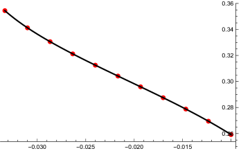
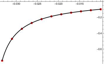
Figure 1: Values of the coefficients $\mu_{0}$ (left) and $\mu_{1}$ (right) in (3.70), for different values of $z$ in the range $-\frac{1}{27}<z<0$ and for a fixed value ${\mathsf{b}}=\pi$, extracted from the asymptotic behaviour of ${\cal F}_{g}({\mathsf{b}})$ up to $g=35$ (after using three Richardson transforms to improve convergence). The numerical values are very close to the theoretical predictions shown in black lines, with $10^{-10}$ and $10^{-9}$ accuracy for $\mu_{0}$ and $\mu_{1}$, respectively.

4 Refined dual partition functions

In this section, we propose an extension of the notion of dual partition function, realized as certain generalized theta series encoding five-brane instantons, that incorporates the refinement. The construction relies on the use of a non-commutative Moyal star product and its extension to the realm of contact geometry. Our main result is that the same Stokes automorphism (3.64) that governs the refined topological string also arises as the transformation of the kernel of the refined dual partition function induced by a non-commutative wall-crossing transformation. Furthermore, by considering higher five-brane charge $k>1$, we obtain a vector-valued generalization of (3.64), which realizes the double quantization proposed in (Alexandrov:2015xir, , §4).

4.1 Five-brane instanton corrections and dual partition functions

Let us first revisit the construction of dual partition functions and their behavior under wall-crossing from Alexandrov:2015xir . This construction can be motivated by considering five-brane instanton corrections to the vector multiplet moduli space ${\cal M}$ arising by compactifying type IIA strings on $X\times S_{1}$ down to 3 dimensions. When $X$ is a compact CY threefold, ${\cal M}$ is a quaternion-Kähler (QK) manifold of real dimension $4b_{2}(X)+4$, of the form

$${\cal M}\simeq{\mathbb{R}}^{+}_{R}\times{\cal S}{\cal K}_{z^{a}}\times{\cal T}_{\zeta^{\Lambda},\tilde{\zeta}_{\Lambda}}\times S^{1}_{\sigma},$$ (4.72)

where ${\mathbb{R}}^{+}$ parametrizes the radius of the circle, ${\cal S}{\cal K}$ the complexified Kähler structure on $X$, ${\cal T}$ the holonomies of the Ramond gauge fields around $H_{\rm even}(X,{\mathbb{Z}})$, and $S^{1}$ the scalar Poincaré-dual to the Kaluza-Klein gauge field in 3 dimensions, and we have indicated in subscript the coordinates used to parametrize the various factors (with $a$ running over $1,\dots,b_{2}:=b_{2}(X)$ and $\Lambda=0,\dots,b_{2}$). Topologically, the level sets of $R$ are principal bundles over ${\cal S}{\cal K}$, whose fibers are twisted tori $\widetilde{{\cal T}}={\mathbb{R}}^{2b_{2}+3}_{\zeta^{\Lambda},\tilde{\zeta}_{\Lambda},\sigma}/\mathds{H}\simeq{\cal T}\times S^{1}$ where $\mathds{H}$ is the Heisenberg group of large gauge transformations parametrized by $\Theta=(\eta^{\Lambda},\tilde{\eta}_{\Lambda},\kappa)\in{\mathbb{Z}}^{2b_{2}+3}$ and acting by

$$\mathscr{T}_{\Theta}\ :\ (\zeta^{\Lambda},\tilde{\zeta}_{\Lambda},\sigma)\ \mapsto\ (\zeta^{\Lambda}+\eta^{\Lambda},\,\tilde{\zeta}_{\Lambda}+\tilde{\eta}_{\Lambda},\,\sigma+2\kappa-\tilde{\eta}_{\Lambda}\zeta^{\Lambda}+\eta^{\Lambda}\tilde{\zeta}_{\Lambda}-\eta^{\Lambda}\tilde{\eta}_{\Lambda}).$$ (4.73)

When $X$ is non-compact, three-dimensional gravity decouples and ${\cal M}$ becomes a family of hyperkähler manifolds of dimension $4b_{2}$ parametrized by the (non-dynamical) radius $R$, of the form ${\cal S}{\cal K}_{z^{a}}\times{\cal T}_{\zeta^{a},\tilde{\zeta}_{a}}$, obtained as rigid limit of (4.72).

As $R\to\infty$, the QK metric on ${\cal M}$ is simply obtained from the special Kähler metric on ${\cal S}{\cal K}$ by the $c$-map construction Ferrara:1989ik , but for finite $R$ there are ${\cal O}(e^{-R})$ corrections from Euclidean D-branes wrapped on even cycles in $X$ times $S^{1}$, and ${\cal O}(e^{-R^{2}})$ corrections from Euclidean five-branes. Both types of corrections must preserve the QK property of the metric, which is equivalent MR1327157 to the existence of a complex contact structure on the twistor space ${\cal Z}\simeq{\mathbb{P}}^{1}_{t}\times{\cal M}$, where the first factor parametrizes the sphere-worth of almost complex structures on ${\cal M}$. Such a structure is guaranteed by the existence of coordinate patches parametrized by complex Darboux coordinates $\xi^{\Lambda},\tilde{\xi}_{\Lambda},\tilde{\alpha}$ such that the contact one-form

$${\cal X}=-\frac{1}{2}\left({\rm d}\tilde{\alpha}-\xi^{\Lambda}{\rm d}\tilde{\xi}_{\Lambda}+\tilde{\xi}_{\Lambda}{\rm d}\xi^{\Lambda}\right)$$ (4.74)

is globally well defined up to rescaling by a non-vanishing holomorphic function. The Darboux coordinates are functions of $t,R,z^{a},\zeta^{\Lambda},\tilde{\zeta}_{\Lambda},\sigma$, holomorphic in $t$ in the respective patches, and can be chosen such that the Heisenberg group acts in the same way as in (4.73),

$$\mathscr{T}_{\Theta}\ :\ (\xi^{\Lambda},\tilde{\xi}_{\Lambda},\tilde{\alpha})\ \mapsto\ (\xi^{\Lambda}+\eta^{\Lambda},\,\tilde{\xi}_{\Lambda}+\tilde{\eta}_{\Lambda},\,\tilde{\alpha}+2\kappa-\tilde{\eta}_{\Lambda}\xi^{\Lambda}+\eta^{\Lambda}\tilde{\xi}_{\Lambda}-\eta^{\Lambda}\tilde{\eta}_{\Lambda}).$$ (4.75)

This is an example of contact transformation, i.e. preserving the contact one-form (4.74). As a result, the twistor space ${\cal Z}$ can be obtained by gluing together algebraic twisted tori $\widetilde{{\cal T}}_{{\mathbb{C}}}={\mathbb{C}}^{2b_{2}+3}_{\xi^{\Lambda},\tilde{\xi}_{\Lambda},\alpha}/H$. The latter admit a projection to algebraic tori ${{\cal T}}_{{\mathbb{C}}}={\mathbb{C}}^{2b_{2}+2}_{\xi^{\Lambda},\tilde{\xi}_{\Lambda}}$, with ${\mathbb{C}}^{\times}$ fiber parametrized by $e^{-\pi{\rm i}\tilde{\alpha}}$.

D-brane instantons are labelled by charge $\gamma=(p^{\Lambda},q_{\Lambda})\in H_{\rm even}(X,{\mathbb{Z}})$ and generate corrections to the QK metric on ${\cal M}$ that can be incorporated at the non-linear level by postulating discontinuities of the Darboux coordinates across the so-called BPS rays $\ell_{\gamma}$ on ${\mathbb{P}}^{1}_{t}$ (the latter being the loci where the phase of $t$ coincides with the central charge $Z(\gamma)$). Namely, one requires that across $\ell_{\gamma}$ they change as Alexandrov:2008gh ; Alexandrov:2009zh ; Alexandrov:2011ac

$$\mathscr{V}_{\gamma}\ :\ \begin{array}[]{rcl}\xi^{\Lambda}&\ \mapsto&\xi^{\prime\Lambda}=\xi^{\Lambda}+\frac{p^{\Lambda}}{2\pi{\rm i}}\,\Omega(\gamma)\,\log\left(1-{\cal X}_{\gamma}\right),\\ \tilde{\xi}_{\Lambda}&\ \mapsto&\tilde{\xi}^{\prime}_{\Lambda}=\tilde{\xi}_{\Lambda}+\frac{q_{\Lambda}}{2\pi{\rm i}}\,\Omega(\gamma)\,\log\left(1-{\cal X}_{\gamma}\right),\\ \tilde{\alpha}&\ \mapsto&\tilde{\alpha}^{\prime}=\tilde{\alpha}+\frac{1}{2\pi^{2}}\,\Omega(\gamma)\,L_{\sigma(\gamma)}({\cal X}_{\gamma}).\end{array}$$ (4.76)

Here $\Omega(\gamma)$ is the generalized DT invariant counting BPS states of charge $\gamma$ in four dimensions, ${\cal X}_{\gamma}=\sigma(\gamma)e^{-2\pi{\rm i}(q_{\Lambda}\xi^{\Lambda}-p^{\Lambda}\tilde{\xi}_{\Lambda})}$ are the twisted Fourier modes, with $\sigma(\gamma)$ a quadratic refinement of the symplectic intersection pairing $\langle\gamma,\gamma^{\prime}\rangle$ on the lattice of charges such that

$${\cal X}_{\gamma}\,{\cal X}_{\gamma^{\prime}}=(-1)^{\langle\gamma,\gamma^{\prime}\rangle}{\cal X}_{\gamma+\gamma^{\prime}},$$ (4.77)

and $L_{\sigma}(z)$ is the twisted Rogers dilogarithm

$$L_{\epsilon}(z)={\rm Li}_{2}(z)+\frac{1}{2}\,\log(\epsilon^{-1}z)\log(1-z)\,.$$ (4.78)

Forgetting the action on $\tilde{\alpha}$, the transformation (4.76) can be written in terms of the Fourier modes ${\cal X}_{\gamma}$ as

$$\mathscr{U}_{\gamma}\ :\ {\cal X}_{\gamma^{\prime}}\ \mapsto\ {\cal X}^{\prime}_{\gamma^{\prime}}={\cal X}_{\gamma^{\prime}}(1-{\cal X}_{\gamma})^{\langle\gamma,\gamma^{\prime}\rangle\Omega(\gamma)}.$$ (4.79)

This is recognized as the Kontsevich-Soibelman (KS) symplectomorphism encoding wall-crossing transformations KS:stability ; Gaiotto:2008cd , or the Delabaere-Dillinger-Pham (DDP) formula controlling the Stokes automorphisms for quantum periods DDP93 . The action on the additional coordinate $\tilde{\alpha}$ lifts $\mathscr{U}_{\gamma}$ to a contact transformation $\mathscr{V}_{\gamma}$. The gluing conditions for $\tilde{\alpha}$ further imply that $e^{-\pi{\rm i}\tilde{\alpha}}$ is a section of the theta line bundle ${\cal L}$ over the algebraic tori ${\cal T}_{\mathbb{C}}$ Alexandrov:2010ca ; Neitzke:2011za . The theta line bundle descends to a canonical hyperholomorphic line bundle over the hyperkähler space obtained from the D-instanton corrected QK space ${\cal M}_{D}$ by the QK/HK correspondence Alexandrov:2011ac .

In contrast, five-brane instanton corrections are poorly understood, beyond linear order around the D-instanton corrected twistor space ${\cal Z}_{D}$ Alexandrov:2010ca (see also Alexandrov:2014mfa ; Alexandrov:2014rca ; Alexandrov:2023hiv ). At linear order, instanton corrections from charge $k$ five-branes are described by sections of ${\cal L}^{k}$, the $k$-th power of the theta line bundle ${\cal L}$. In practice, this means that on local coordinate patches they are described by functions $H_{k}(\xi,\tilde{\xi},\tilde{\alpha}):=e^{-{\rm i}\pi k\tilde{\alpha}}H_{k}(\xi,\tilde{\xi})$ which stay invariant under the contact transformations $\mathscr{T}_{\Theta}$ and are mapped to each other under $\mathscr{V}_{\gamma}$.

The invariance under the Heisenberg action (4.75) requires that

$$H_{k}(\xi+\eta,\tilde{\xi}+\tilde{\eta})=(-1)^{k\eta^{\Lambda}\tilde{\eta}_{\Lambda}}e^{\pi{\rm i}k(\eta^{\Lambda}\tilde{\xi}_{\Lambda}-\tilde{\eta}_{\Lambda}\xi^{\Lambda})}\,H_{k}(\xi,\tilde{\xi}).$$ (4.80)

This implies the following ‘non-Abelian’ Fourier expansion

$$H_{k}(\xi,\tilde{\xi},\tilde{\alpha})=\sum_{\ell^{\Lambda}\in\frac{{\mathbb{Z}}^{b_{2}}}{|k|{\mathbb{Z}}^{b_{2}}}}\sum_{n^{\Lambda}\in{\mathbb{Z}}^{b_{2}}+\frac{\ell^{\Lambda}}{k}}e^{-\pi{\rm i}k(\tilde{\alpha}+\xi^{\Lambda}\tilde{\xi}_{\Lambda})+2\pi{\rm i}kn^{\Lambda}\tilde{\xi}_{\Lambda}}\,{\cal H}_{k,\ell^{\Lambda}}(\xi^{\Lambda}-n^{\Lambda})\,,$$ (4.81)

where ${\cal H}_{k,\ell^{\Lambda}}(\xi^{\Lambda})$ is referred to as the wave-function. The reason for this terminology is that it transforms in the metaplectic representation under a change of symplectic basis. For example, upon exchanging the ’position’ coordinates $\xi^{\Lambda}$ with the conjugate ’momenta’ $\tilde{\xi}_{\Lambda}$, one gets

$$H_{k}(\xi,\tilde{\xi},\tilde{\alpha})=\sum_{l_{\Lambda}\in\frac{{\mathbb{Z}}}{|k|{\mathbb{Z}}}}\sum_{m_{\Lambda}\in{\mathbb{Z}}+\frac{\ell^{\Lambda}}{k}}e^{-\pi{\rm i}k(\tilde{\alpha}-\xi^{\Lambda}\tilde{\xi}_{\Lambda})-2\pi{\rm i}km_{\Lambda}\xi^{\Lambda}}\,{\cal H}^{\prime}_{k,l_{\Lambda}}(\tilde{\xi}_{\Lambda}-m_{\Lambda})\,,$$ (4.82)

where the wave-functions are related by Fourier transform

$${\cal H}_{k,\ell^{\Lambda}}(\xi)=\sum_{m_{\Lambda}\in\frac{{\mathbb{Z}}}{|k|{\mathbb{Z}}}}e^{-2\pi{\rm i}m_{\Lambda}\ell^{\Lambda}/k}\int{\rm d}\tilde{\xi}_{\Lambda}\,e^{2\pi{\rm i}k\xi^{\Lambda}\tilde{\xi}_{\Lambda}}\,{\cal H}^{\prime}_{k,m_{\Lambda}}(\tilde{\xi})\,.$$ (4.83)

For $k=1$, it was argued in Alexandrov:2010ca using S-duality in type IIB string theory that the wave function ${\cal H}_{1}(\xi)$ should be identified with the topological string partition function in real polarization ${\cal Z}_{{\mathbb{R}}}(\xi)$, analytically continued to the complex domain and evaluated on the Darboux coordinates $\xi^{\Lambda}$. As a result, (4.81) becomes proportional to the ‘dual partition function’:

$$H_{1}(\xi,\tilde{\xi},\tilde{\alpha})=e^{2\pi{\rm i}\alpha}\sum_{n^{\Lambda}\in{\mathbb{Z}}}e^{2\pi{\rm i}n^{\Lambda}\tilde{\xi}_{\Lambda}}{\cal Z}_{{\mathbb{R}}}(\xi^{\Lambda}-n^{\Lambda})\,,$$ (4.84)

where we introduced

$$\alpha=-\frac{1}{2}\,(\tilde{\alpha}+\xi^{\Lambda}\tilde{\xi}_{\Lambda})$$ (4.85)

such that

$${\cal X}={\rm d}\alpha+\xi^{\Lambda}{\rm d}\tilde{\xi}_{\Lambda}.$$ (4.86)

In fact, ${\cal Z}_{{\mathbb{R}}}(\xi)$ can be shown to be proportional to the usual holomorphic topological string partition function ${\cal Z}(\boldsymbol{t};g_{s})$ provided one identifies

$$t^{a}=2\pi{\rm i}\,\frac{\xi^{a}}{\xi^{0}}\,,\qquad g_{s}=\frac{2\pi}{\xi^{0}}\,.$$ (4.87)

Thus, the five-brane instantons turn out to be described by the unrefined version of the partition function studied in the previous sections.

One of the main results of Alexandrov:2015xir was to determine the transformation property of the wave functions ${\cal H}_{k,\ell^{\Lambda}}$ under the contact transformations (4.76). Taking into account the transformation of $\tilde{\alpha}$, it is immediate to see that

$$\mathscr{V}_{\gamma}\ :\ H_{k}(\xi,\tilde{\xi})\ \mapsto\ H^{\prime}_{k}(\xi,\tilde{\xi})=e^{\frac{k}{2\pi{\rm i}}\,\Omega(\gamma)\,L_{\sigma(\gamma)}({\cal X}_{\gamma})}\,H_{k}(\xi^{\prime},\tilde{\xi}^{\prime})\,.$$ (4.88)

In the pure electric case $\gamma=(0,q^{\Lambda})$, it was shown that this implies

$$\mathscr{V}_{\gamma}\ :\ {\cal H}_{k,\ell^{\Lambda}}(\xi)\ \mapsto\ \left[\mathbf{A}^{(k)}(-q_{\Lambda}\xi^{\Lambda},-q_{\Lambda}\ell^{\Lambda})\right]^{-\Omega(\gamma)}\,{\cal H}_{k,\ell^{\Lambda}}(\xi),$$ (4.89)

where

$$\mathbf{A}^{(k)}(x,\ell)=\left(1-e^{2\pi{\rm i}(x+\ell/k)}\right)^{\ell}\,\bigl{[}\Phi_{1}\left({\rm i}(x+\ell/k)\right)\bigr{]}^{k}.$$ (4.90)

The transformation property across generic BPS rays can be obtained by conjugating (4.89) by the metaplectic representation, or by extending by a rank 2 hyperbolic lattice, see (Alexandrov:2015xir, , (2.11)). For $k=1$, (4.89) and (4.87) imply that the topological string amplitude ${\cal Z}(\boldsymbol{t};g_{s})$ gets multiplied by $\Phi_{1}\left(-(q_{a}t^{a}+2\pi{\rm i}q_{0})/g_{s}\right)$, which coincides with the Stokes factor for the topological string partition function, as noticed in Iwaki:2023cek .

4.2 Refined contact structure

Our goal is to incorporate the refinement parameter into the above construction. In fact, a refined version of the function $\mathbf{A}^{(k)}(x,\ell)$ was already put forward in (Alexandrov:2015xir, , §4). However, it was not derived nor justified by any invariance or transformation property. To fill this gap, we have to find a proper generalization of the dual partition function (4.84) (or more generally (4.81)) and compute the action of a refined version of the transformation $\mathscr{V}_{\gamma}$ (4.76) on its kernel. However, as will be discussed shortly, while the refinement of the symplectomorphism $\mathscr{U}_{\gamma}$ is well understood, this is not so for the contact transformation $\mathscr{V}_{\gamma}$. Therefore, the first step is to find how to lift refined symplectomorphisms to refined contact transformations. Since the defining property of the latter in the absence of refinement was that they preserve the contact one-form, this can be seen as constructing a refined version of the contact structure. This is the problem that we address in this subsection.

Physically, the standard way to introduce a refinement is to switch on an $\Omega$-background. As was observed in Gaiotto:2010be ; Cecotti:2014wea in the gauge theory context, its effect is to deform the Riemann-Hilbert problem defining the instanton-corrected metric on the Coulomb branch into a non-commutative one Barbieri:2019yya . This is achieved by replacing the KS symplectomorphism (4.79) by its quantum version

$$\hat{\mathscr{U}}_{\gamma}\ :\ {\cal X}_{\gamma^{\prime}}\ \mapsto\ {\cal X}^{\prime}_{\gamma^{\prime}}={\cal U}_{\gamma}\star{\cal X}_{\gamma^{\prime}}\star{\cal U}_{\gamma}^{-1}.$$ (4.91)

Here $\star$ denotes the non-commutative Moyal product

$$f\star g=f\exp\left[\frac{{\rm i}\,\epsilon}{2\pi}\sum_{\Lambda}\left(\overleftarrow{\partial}_{\!\xi^{\Lambda}}\overrightarrow{\partial}_{\!\tilde{\xi}_{\Lambda}}-\overleftarrow{\partial}_{\!\tilde{\xi}_{\Lambda}}\overrightarrow{\partial}_{\!\xi^{\Lambda}}\right)\right]g,$$ (4.92)

where $\epsilon$ is the refinement parameter to be related to ${\mathsf{b}}$ in the next subsection. It is easy to check that with respect to the Moyal product the relation (4.77) gets deformed to

$${\cal X}_{\gamma}\star{\cal X}_{\gamma^{\prime}}=(-y)^{\langle\gamma,\gamma^{\prime}\rangle}{\cal X}_{\gamma+\gamma^{\prime}},\qquad y=e^{2\pi{\rm i}\epsilon}.$$ (4.93)

The function ${\cal U}_{\gamma}$ in (4.91), which generates the quantum KS transformation, is defined in terms the compact quantum dilogarithm $E_{y}(x)$, described in Appendix A, as

$${\cal U}_{\gamma}=\prod_{n\in{\mathbb{Z}}}E_{y}\left(y^{n}\,{\cal X}_{\gamma}\right)^{\Omega_{n}(\gamma)},$$ (4.94)

where $\Omega_{n}(\gamma)$ are the Laurent coefficients of the refined BPS indices (to be distinguished from the multiplicities $\Omega_{[j]}(\gamma)$ defined in (2.25))

$$\Omega(\gamma,y)=\sum_{n\in{\mathbb{Z}}}\Omega_{n}(\gamma)\,y^{n}.$$ (4.95)

Note that the product in (4.94) is finite, since $\Omega_{n}(\gamma)$ vanishes for $|n|$ large enough. Substituting (4.94) into (4.91) and evaluating the star product explicitly, one finds

$$\begin{split}{\cal X}^{\prime}_{\gamma^{\prime}}=&\,{\cal X}_{\gamma^{\prime}}\prod_{n\in{\mathbb{Z}}}\left[\frac{E_{y}\left(y^{n+\langle\gamma,\gamma^{\prime}\rangle}\,{\cal X}_{\gamma}\right)}{E_{y}\left(y^{n-\langle\gamma,\gamma^{\prime}\rangle}\,{\cal X}_{\gamma}\right)}\right]^{\Omega_{n}(\gamma)}\\ =&\,{\cal X}_{\gamma^{\prime}}\prod_{n\in{\mathbb{Z}}}\prod_{k=0}^{|\langle\gamma,\gamma^{\prime}\rangle|-1}\left(1-y^{n+2k-|\langle\gamma,\gamma^{\prime}\rangle|+1}{\cal X}_{\gamma}\right)^{{\rm sgn}\langle\gamma,\gamma^{\prime}\rangle\,\Omega_{n}(\gamma)}\,,\end{split}$$ (4.96)

where in the second step we used the property (A.131) of the quantum dilogarithm. In the unrefined limit $y\to 1$, this transformation reduces to the classical symplectomorphism (4.79), as it should.

The analysis of Alexandrov:2019rth suggests that a similar non-commutative deformation is induced by the refinement in full string theory as well. But in this case we also need to understand how to extend $\hat{\mathscr{U}}_{\gamma}$ to act on the full twistor space, including the coordinate $\tilde{\alpha}$. In other words, we need to extend the construction to the case of twisted quantum tori. To this end, we observe that the contact one-form (4.86) on $\widetilde{\cal T}_{{\mathbb{C}}}$ arises by projectivizing the symplectic form $\omega$ on a ${\mathbb{C}}^{\star}$ bundle over $\widetilde{\cal T}_{{\mathbb{C}}}$ (which coincides at least locally with the Swann bundle MR1096180 of the QK space ${\cal M}$), with Darboux coordinates $(\eta^{I},\mu_{I})$, $I=\flat,0,\dots,b_{2}$, such that Alexandrov:2010qdt

$$\omega=\sum_{I}{\rm d}\eta^{I}\wedge{\rm d}\mu_{I}\,.$$ (4.97)

Indeed, under the identification

$$\xi^{\Lambda}=\frac{\eta^{\Lambda}}{\eta^{\flat}}\,,\qquad\tilde{\xi}_{\Lambda}=\mu_{\Lambda}\,,\qquad\alpha=\mu_{\flat}\,,$$ (4.98)

we have

$$\omega={\rm d}\eta^{\flat}\wedge({\rm d}\mu_{\flat}+\xi^{\Lambda}{\rm d}\tilde{\xi}_{\Lambda})+\eta^{\flat}{\rm d}\xi^{\Lambda}\wedge{\rm d}\tilde{\xi}_{\Lambda}={\rm d}\eta^{\flat}\wedge{\cal X}+\eta^{\flat}{\rm d}{\cal X}.$$ (4.99)

Thus, we can define a star product on functions of $\xi^{\Lambda},\tilde{\xi}_{\Lambda},\alpha$ (or equivalently functions of $\xi^{\Lambda},\mu_{I}$) by viewing them as functions of $(\eta^{I},\mu_{I})$ which are invariant under the ${\mathbb{C}}^{\times}$ action $\eta^{I}\to\lambda\eta^{I}$, and using the Moyal product on ${\mathbb{C}}^{2b_{2}+4}$, with a deformation parameter that we denote by $\epsilon^{\flat}$,

$$f\star g=f\exp\left[\frac{{\rm i}\,\epsilon^{\flat}}{2\pi}\sum_{I}\left(\overleftarrow{\partial}_{\!\eta^{I}}\overrightarrow{\partial}_{\!\mu_{I}}-\overleftarrow{\partial}_{\!\mu_{I}}\overrightarrow{\partial}_{\!\eta^{I}}\right)\right]g.$$ (4.100)

In general, the resulting Moyal product is not invariant under the ${\mathbb{C}}^{\times}$ action $\eta^{I}\to\lambda\eta^{I}$, unless this action also affects the deformation parameter via $\epsilon^{\flat}\to\lambda\epsilon^{\flat}$. In other words, the result is not only a function of $\xi^{\Lambda}\equiv\eta^{\Lambda}/\eta^{\flat}$ and $\mu_{I}$ but also depends on $\epsilon\equiv\epsilon^{\flat}/\eta^{\flat}$. Thus, the Moyal product (4.100) defines a non-commutative deformation of the product of functions $f(\xi^{\Lambda},\tilde{\xi}_{\Lambda},\tilde{\alpha},\epsilon)$ on $\widetilde{T}_{{\mathbb{C}}}\times{\mathbb{C}}_{\epsilon}$, which by construction preserves associativity.

It is easy to see that the corresponding Moyal bracket

$$\{f,g\}_{\star}=\frac{\pi}{{\rm i}\epsilon}\left(f\star g-g\star f\right)$$ (4.101)

in the unrefined limit $\epsilon\to 0$ reproduces the contact bracket $\{\,\cdot\,,\,\cdot\,\}_{0,0}$ introduced in Alexandrov:2008gh . Since the latter essentially encodes the contact structure, e.g. it generates classical contact transformations via exponentiation $\exp\{h,\,\cdot\,\}_{1,0}$ Alexandrov:2014mfa , the star product (4.100) can be thought as providing a definition of the refined contact structure.

4.3 Wave functions and non-commutative wall-crossing

Equipped with the star product, we can now construct a refined analogue of the dual partition function (4.81). To this end, we simply replace the usual product by the non-commutative one,

$$H^{\text{(ref)}}_{k}(\xi,\tilde{\xi},\alpha)=\sum_{\ell^{\Lambda}\in\frac{{\mathbb{Z}}}{|k|{\mathbb{Z}}}}\sum_{n^{\Lambda}\in{\mathbb{Z}}+\ell^{\Lambda}/k}e^{2\pi{\rm i}k(\alpha+n^{\Lambda}\tilde{\xi}_{\Lambda})}\star{\cal H}^{\text{(ref)}}_{k,\ell^{\Lambda}}(\xi^{\Lambda}-n^{\Lambda}).$$ (4.102)

In fact, the star product can be evaluated explicitly using the property

$$e^{2\pi{\rm i}(k\alpha+p^{\Lambda}\tilde{\xi}_{\Lambda})}\star f(\xi^{\Lambda},\tilde{\xi}_{\Lambda},\alpha,\epsilon)=e^{2\pi{\rm i}(k\alpha+p^{\Lambda}\tilde{\xi}_{\Lambda})}\,f\left(\frac{\xi^{\Lambda}+\epsilon p^{\Lambda}}{1+\epsilon k},\tilde{\xi}_{\Lambda},\alpha,\frac{\epsilon}{1+\epsilon k}\right).$$ (4.103)

In particular, it allows to see that the invariance under the Heisenberg group still holds. Indeed, the star product changes the argument of ${\cal H}^{\text{(ref)}}_{k,\ell^{\Lambda}}$ to $\frac{\xi^{\Lambda}+k\epsilon n^{\Lambda}}{1+k\epsilon}-n^{\Lambda}=\frac{\xi^{\Lambda}-n^{\Lambda}}{1+k\epsilon}$ and thus the refined wave function is still a function of the difference $\xi^{\Lambda}-n^{\Lambda}$, which ensures the invariance.

Our goal now is to determine the transformation property of the refined wave-function ${\cal H}^{\text{(ref)}}_{k,\ell}(\xi)$ under the quantum KS transformations $\hat{\mathscr{U}}_{\gamma}$ lifted to the twisted torus by means of (4.100). Denoting by $\hat{\mathscr{V}}_{\gamma}$ the corresponding lift, we arrive at the following condition

$$\sum_{\ell^{\Lambda},n^{\Lambda}}e^{2\pi{\rm i}k(\alpha+n^{\Lambda}\tilde{\xi}_{\Lambda})}\star\hat{\mathscr{V}}_{\gamma}[{\cal H}^{\text{(ref)}}_{k,\ell^{\Lambda}}(\xi-n)]={\cal U}_{\gamma}\star\sum_{\ell^{\Lambda},n^{\Lambda}}e^{2\pi{\rm i}k(\alpha+n^{\Lambda}\tilde{\xi}_{\Lambda})}\star{\cal H}^{\text{(ref)}}_{k,\ell^{\Lambda}}(\xi-n)\star{\cal U}_{\gamma}^{-1}.$$ (4.104)

Restricting to the electric case $\gamma=(0,q_{\Lambda})$, such that ${\cal U}_{\gamma}$ becomes a function of $\xi^{\Lambda}$ and $\epsilon$ only and therefore commutes with the wave function, and using (4.103) to evaluate the star product, we obtain that the r.h.s. of (4.104) is given by

$$\sum_{\ell^{\Lambda},n^{\Lambda}}e^{2\pi{\rm i}k(\alpha+n^{\Lambda}\tilde{\xi}_{\Lambda})}\star\frac{{\cal U}_{\gamma}\left(\frac{\xi-2k\epsilon n}{1-2k\epsilon};\frac{\epsilon}{1-2k\epsilon}\right)}{{\cal U}_{\gamma}(\xi;\epsilon)}\,{\cal H}^{\text{(ref)}}_{k,\ell^{\Lambda}}(\xi-n).$$ (4.105)

Furthermore, using that

$$\begin{split}e^{-2\pi{\rm i}q_{\Lambda}\xi^{\Lambda}}=&\,e^{-2\pi{\rm i}q_{\Lambda}(\xi^{\Lambda}-n^{\Lambda}+\ell^{\Lambda}/k)},\\ e^{-2\pi{\rm i}q_{\Lambda}\,\frac{\xi^{\Lambda}-2k\epsilon n^{\Lambda}}{1-2k\epsilon}}=&\,e^{-2\pi{\rm i}q_{\Lambda}\left(\frac{\xi^{\Lambda}-n^{\Lambda}}{1-2k\epsilon}+\frac{\ell^{\Lambda}}{k}\right)},\end{split}$$ (4.106)

it is easy to see that the factor generated by the transformation depends on $\xi^{\Lambda}$ and $n^{\Lambda}$ only through their difference. Thus, the condition (4.104) requires that the wave function should transform as

$$\hat{\mathscr{V}}_{\gamma}[{\cal H}^{\text{(ref)}}_{k,\ell^{\Lambda}}(\xi)]=\Upsilon_{k,\ell^{\Lambda}}(\xi)\,{\cal H}^{\text{(ref)}}_{k,\ell^{\Lambda}}(\xi),\qquad\Upsilon_{k,\ell^{\Lambda}}(\xi)=\frac{{\cal U}_{\gamma}\left(\frac{\xi}{1-2k\epsilon}+\frac{\ell}{k}\,;\,\frac{\epsilon}{1-2k\epsilon}\right)}{{\cal U}_{\gamma}(\xi+\ell/k;\epsilon)}\,.$$ (4.107)

It turns out that the function $\Upsilon_{k,\ell^{\Lambda}}$ can be expressed through the Faddeev quantum dilogarithm or its appropriate generalization, which are all described in Appendix A. For simplicity, let us first consider the unit multiplicity case, $\Omega_{n}(\gamma)=\delta_{n}$, such that

$${\cal U}_{\gamma}(\xi;\epsilon)=E_{y}\left(e^{-2\pi{\rm i}q_{\Lambda}\xi^{\Lambda}}\right)$$ (4.108)

with $y=e^{2\pi{\rm i}\epsilon}$. We will distinguish between cases of positive and negative five-brane charge $k$ because they lead to different relations between the refinement parameters $\epsilon$ and ${\mathsf{b}}$. For $k>0$, we identify

$$\epsilon=\frac{1}{2k}\left(1-{\mathsf{b}}^{-2}\right),$$ (4.109)

such that $1-2k\epsilon={\mathsf{b}}^{-2}$ and

$$y=e^{\pi{\rm i}/k}e^{-\pi{\rm i}/({\mathsf{b}}^{2}k)}:={\tilde{y}}_{{\mathsf{b}},k},\qquad e^{\frac{2\pi{\rm i}\epsilon}{1-2k\epsilon}}=e^{-\pi{\rm i}/k}e^{\pi{\rm i}{\mathsf{b}}^{2}/k}:=y_{{\mathsf{b}},k}.$$ (4.110)

which generalize the variables (3.54) to generic $k$ and satisfy ${\tilde{y}}_{{\mathsf{b}},k}=\bar{y}_{1/\bar{\mathsf{b}},k}$. Thus, the function $\Upsilon_{k,\ell^{\Lambda}}$ in (4.107) takes the form

$$\Upsilon_{k,\ell^{\Lambda}}(\xi)=\frac{E_{y_{{\mathsf{b}},k}}\left(e^{-2\pi{\rm i}({\mathsf{b}}^{2}q_{\Lambda}\xi^{\Lambda}+\ell/k)}\right)}{E_{{\tilde{y}}_{{\mathsf{b}},k}}\left(e^{-2\pi{\rm i}(q_{\Lambda}\xi^{\Lambda}+\ell/k)}\right)}\,,$$ (4.111)

where we denoted $\ell=q_{\Lambda}\ell^{\Lambda}$. Setting also $s_{\ell}={\rm sgn}(\ell)$ and using (A.131), the numerator can be rewritten as

$$E_{y_{{\mathsf{b}},k}}\left(y_{{\mathsf{b}},k}^{2\ell}\,e^{-2\pi{\rm i}{\mathsf{b}}^{2}(q_{\Lambda}\xi^{\Lambda}+\ell/k)}\right)=E_{y_{{\mathsf{b}},k}}\left(e^{-2\pi{\rm i}{\mathsf{b}}^{2}(q_{\Lambda}\xi^{\Lambda}+\ell/k)}\right)\prod_{j=0}^{|\ell|-1}\left(1-y_{{\mathsf{b}},k}^{2\ell-s_{\ell}(2j+1)}\,e^{-2\pi{\rm i}{\mathsf{b}}^{2}(q_{\Lambda}\xi^{\Lambda}+\ell/k)}\right)^{s_{\ell}}.$$ (4.112)

We can then use the property (A.130) to get

$$\displaystyle\Upsilon_{k,\ell^{\Lambda}}(\xi) = \prod_{j=0}^{k-1}\frac{E_{e^{\pi{\rm i}{\mathsf{b}}^{2}}}\left(-e^{-2\pi{\rm i}{\mathsf{b}}\,\Xi^{+}_{k,j}}\right)}{E_{e^{-\pi{\rm i}/{\mathsf{b}}^{2}}}\left(-e^{-2\pi{\rm i}{\mathsf{b}}^{-1}\,\Xi^{+}_{k,j}}\right)}\prod_{j=0}^{|\ell|-1}\left(1-e^{-2\pi{\rm i}\left({\mathsf{b}}^{2}q_{\Lambda}\xi^{\Lambda}+\frac{\ell}{k}+\frac{s_{\ell}}{k}({\mathsf{b}}^{2}-1)\left(j+\frac{1}{2}\right)\right)}\right)^{s_{\ell}}$$ (4.113)

$$= \prod_{j=0}^{k-1}\Phi_{\mathsf{b}}^{-1}(-{\rm i}\Xi^{+}_{k,j})\prod_{j=0}^{|\ell|-1}\left(1-e^{-2\pi{\rm i}\left({\mathsf{b}}^{2}q_{\Lambda}\xi^{\Lambda}+\frac{\ell}{k}+\frac{s_{\ell}}{k}({\mathsf{b}}^{2}-1)\left(j+\frac{1}{2}\right)\right)}\right)^{s_{\ell}},$$

where

$$\Xi^{+}_{k,j}={\mathsf{b}}q_{\Lambda}\xi^{\Lambda}+\frac{{\mathsf{b}}\ell}{k}-\frac{1}{k}\left({\mathsf{b}}-{\mathsf{b}}^{-1}\right)\left(j-\frac{k-1}{2}\right).$$ (4.114)

For $\ell>0$ (hence $s=1$), (4.113) is recognized as the function ${\bf A}_{\hbar}^{(k)}(t,\ell)$ defined in (Alexandrov:2015xir, , (4.1)) evaluated at $\hbar={\mathsf{b}}^{2}$ and $t=-{\rm i}{\mathsf{b}}^{2}q_{\Lambda}\xi^{\Lambda}$.

For $k<0$, we replace the identification (4.109) by

$$\epsilon=\frac{1}{2k}(1-{\mathsf{b}}^{2}),$$ (4.115)

such that $1-2k\epsilon={\mathsf{b}}^{2}$ and

$$y=y_{{\mathsf{b}},-k},\qquad e^{\frac{2\pi{\rm i}\epsilon}{1-2k\epsilon}}={\tilde{y}}_{{\mathsf{b}},-k}.$$ (4.116)

Repeating the same steps as above, one arrives at the following representation for the function $\Upsilon_{k,\ell^{\Lambda}}$ (4.107):

$$\displaystyle\Upsilon_{k,\ell^{\Lambda}}(\xi) = \prod_{j=0}^{|k|-1}\Phi_{\mathsf{b}}(-{\rm i}\Xi^{-}_{k,j})\prod_{j=0}^{|\ell|-1}\left(1-e^{-2\pi{\rm i}\left({\mathsf{b}}^{-2}q_{\Lambda}\xi^{\Lambda}+\frac{\ell}{k}+\frac{s_{\ell}}{k}({\mathsf{b}}^{-2}-1)\left(j+\frac{1}{2}\right)\right)}\right)^{s_{\ell}},$$ (4.117)

where now

$$\Xi^{-}_{k,j}={\mathsf{b}}^{-1}q_{\Lambda}\xi^{\Lambda}+\frac{\ell}{{\mathsf{b}}k}-\frac{1}{|k|}\left({\mathsf{b}}-{\mathsf{b}}^{-1}\right)\left(j-\frac{|k|-1}{2}\right).$$ (4.118)

For BPS rays carrying general refined BPS indices $\Omega_{n}(\gamma)$, the wall-crossing transformation can be expressed through a generalization $\Phi^{[j],k}_{{\mathsf{b}}}(z)$ of the Faddeev quantum dilogarithm defined in (A.144), which also has a representation as a product of the usual quantum dilogarithms with shifted arguments. Again, proceeding as above, it is straightforward to show that

$$\Upsilon_{k,\ell^{\Lambda}}(\xi)=\prod_{j}\left[\prod_{i=0}^{|k|-1}\left(\Phi^{[j],k}_{{\mathsf{b}}}(-{\rm i}\Xi^{s_{k}}_{k,i})\right)^{s_{k}}\prod_{m=-j}^{j}\prod_{i=0}^{|\ell|-1}\left(1-e^{-2\pi{\rm i}\left({\mathsf{b}}^{2s_{k}}q_{\Lambda}\xi^{\Lambda}+\frac{\ell}{k}+\frac{s_{\ell}}{k}({\mathsf{b}}^{2s_{k}}-1)\left(i-m+\frac{1}{2}\right)\right)}\right)^{-s_{\ell}}\right]^{-\Omega_{[j]}},$$ (4.119)

where $s_{k}={\rm sgn}(k)$. For $k=1$, in which case $\ell=0$, this formula reduces to

$$\Upsilon_{1}(\xi)=\prod_{j}\left[\Phi_{{\mathsf{b}}}^{[j]}(-{\rm i}{\mathsf{b}}q_{\Lambda}\xi^{\Lambda})\right]^{-\Omega_{[j]}}.$$ (4.120)

This result is to be compared with (3.64) where ${\cal A}=2\pi q_{a}t^{a}+4\pi^{2}{\rm i}q_{0}$. It s easy to see that the factor appearing in (3.64) coincides with $\Upsilon_{1}(\xi)$ provided one relates the variables as in (4.87) with $\xi^{\Lambda}$ replaced by ${\mathsf{b}}\xi^{\Lambda}$, i.e.

$$t^{a}=2\pi{\rm i}\,\frac{\xi^{a}}{\xi^{0}}\,,\qquad g_{s}=\frac{2\pi}{{\mathsf{b}}\xi^{0}}\,.$$ (4.121)

Note that the last relation is equivalent to

$$\xi^{0}=\frac{2\pi}{\epsilon_{1}}\,,$$ (4.122)

where $\epsilon_{1}$ is one the deformation parameters of the $\Omega$-background, see (2.1). The match of the Stocks factors suggests that the wave function ${\cal H}^{\text{(ref)}}_{1}$ is proportional to the refined topological string,

$${\cal H}^{\text{(ref)}}_{1}(\xi)\sim{\cal Z}(\boldsymbol{t};g_{s},{\mathsf{b}}),$$ (4.123)

with the parameters identified as in (4.121). This generalizes a similar relation in the unrefined case.

Note that if we had chosen the opposite ordering in the definition of the refined dual partition function (4.102), the results for the cases of positive and negative $k$ would effectively be swapped. Indeed, exchanging the ordering of factors in (4.103) leads to the flip of signs in front of $k$ and $p^{\Lambda}$ in the arguments of the function $f$. As a result, denoting by tilde the quantities corresponding to the opposite ordering, one has

$$\tilde{\Upsilon}_{k,\ell^{\Lambda}}(\xi)=\Upsilon_{-k,-\ell^{\Lambda}}^{-1}(\xi).$$ (4.124)

In particular, using (4.119), one finds that

$$\tilde{\Upsilon}_{1}(\xi)=\prod_{j}\left[\Phi_{{\mathsf{b}}}^{[j]}(-{\rm i}{\mathsf{b}}^{-1}q_{\Lambda}\xi^{\Lambda})\right]^{-\Omega_{[j]}},$$ (4.125)

which in turn implies the identification

$$\tilde{\cal H}^{\text{(ref)}}_{1}(\xi)\sim{\cal Z}\left(2\pi{\rm i}\,\frac{\xi^{a}}{\xi^{0}}\,;\,\frac{2\pi{\mathsf{b}}}{\xi^{0}}\,,{\mathsf{b}}\right).$$ (4.126)

Note that in this case the relation (4.122) is replaced by

$$\xi^{0}=-\frac{2\pi}{\epsilon_{2}}\,.$$ (4.127)

We observe that the effect of the refinement is to introduce a factor of ${\mathsf{b}}$ in the relation between $\xi^{0}$ and the topological string coupling $g_{s}$. It spoils the symmetry ${\mathsf{b}}\leftrightarrow{\mathsf{b}}^{-1}$, unless one simultaneously changes the ordering in the definition of the refined dual partition function. Of course, this factor could be absorbed in the definition of the Darboux coordinates $\xi^{\Lambda}$, but the price to pay is a modification of the quasi-periodicity conditions (4.75) and (4.80), and it would reappear anyway in the quantization condition of charges.

Appendix A Quantum dilogarithms

In this Appendix, we introduce several versions of the quantum dilogarithm function which play a role in this work.

The standard (sometimes called compact) quantum dilogarithm $E_{y}(x)$ is defined as

$$E_{y}(x):=\exp\left[\sum_{k=1}^{\infty}\frac{(xy)^{k}}{k(1-y^{2k})}\right]=\prod_{n=0}^{\infty}(1-xy^{2n+1})^{-1}=(xy;y^{2})_{\infty}^{-1},$$ (A.128)

where the last representation is given in terms of the $q$-Pochhammer symbol $(a;q)_{n}:=\prod_{k=0}^{n-1}(1-aq^{k})$. The quantum dilogarithm satisfies the following properties:

$$\displaystyle E_{y}(xy^{2}) = (1-xy)E_{y}(x),$$ (A.129)

$$E_{y^{1/k}}(x) = \prod_{j=0}^{k-1}E_{y}\left(y^{\frac{2j+1}{k}-1}x\right),\qquad k\in{\mathbb{N}}.$$ (A.130)

The first property has the obvious generalization

$$E_{y}(y^{2\ell}x)=E_{y}(x)\prod_{j=0}^{\ell-1}(1-xy^{2j+1}),\qquad\ell\in{\mathbb{N}}.$$ (A.131)

A different version of the quantum dilogarithm (sometimes called non-compact) is due to Faddeev Faddeev ,

$$\Phi_{\mathsf{b}}(z):=\exp\left(\int_{{\mathbb{R}}+{\rm i}\epsilon}\frac{e^{-2{\rm i}zv}}{4\sinh(v{\mathsf{b}})\sinh(v/{\mathsf{b}})}\frac{{\rm d}v}{v}\right).$$ (A.132)

It possesses several beautiful properties listed, for example, in (Alexandrov:2015xir, , §A.2). Here we mention the quasi-periodicity

$$\Phi_{\mathsf{b}}(x-{\rm i}{\mathsf{b}}^{\pm 1}/2)=\left(1+e^{2\pi{\mathsf{b}}^{\pm 1}x}\right)\Phi_{\mathsf{b}}(x+{\rm i}{\mathsf{b}}^{\pm 1}/2),$$ (A.133)

the classical limit

$$\Phi_{\mathsf{b}}(x)\mathop{\sim}\limits_{{\mathsf{b}}\to 0}\exp\left(\frac{{\rm Li}_{2}(-e^{2\pi{\mathsf{b}}x})}{2\pi{\rm i}{\mathsf{b}}^{2}}\right),$$ (A.134)

the special value at ${\mathsf{b}}=1$

$$\Phi_{1}(x)=\exp\left[\frac{{\rm i}}{2\pi}\left({\rm Li}_{2}(e^{2\pi x})+2\pi x\log(1-e^{2\pi x})\right)\right],$$ (A.135)

and the special value at ${\mathsf{b}}^{2}=2$

$$\Phi_{\sqrt{2}}\left({x\over{\sqrt{2}}}\right)=\exp\left[\frac{{\rm i}}{4\pi}\left({\rm Li}_{2}(-e^{2\pi x})+2\pi x\log(1+e^{2\pi x})+2\pi\tan^{-1}({\rm e}^{\pi x})\right)\right],$$ (A.136)

which follows from the more general results of garkas .

Evaluating the integral in (A.132) by residues, one finds that

$$\log\Phi_{\mathsf{b}}(z)=\sum_{\ell=1}^{\infty}\frac{(-1)^{\ell}}{2{\rm i}\ell}\left(\frac{e^{2\pi\ell z{\mathsf{b}}}}{\sin(\ell\pi{\mathsf{b}}^{2})}+\frac{e^{2\pi\ell z/{\mathsf{b}}}}{\sin(\ell\pi/{\mathsf{b}}^{2})}\right),$$ (A.137)

which allows to establish the following relation between the two versions of quantum dilogarithm (Faddeev:2000if, , §A)

$$\Phi_{\mathsf{b}}(z)=\frac{E_{e^{-{\rm i}\pi/{\mathsf{b}}^{2}}}\left(-e^{2\pi z/{\mathsf{b}}}\right)}{E_{e^{{\rm i}\pi{\mathsf{b}}^{2}}}\left(-e^{2\pi z{\mathsf{b}}}\right)}=\frac{E_{{\tilde{y}}_{\mathsf{b}}}\left(e^{2\pi z/{\mathsf{b}}}\right)}{E_{y_{\mathsf{b}}}\left(e^{2\pi z{\mathsf{b}}}\right)}\,,$$ (A.138)

where in the second representation we used the variables defined in (3.54).

Let us now introduce a generalization of the compact quantum dilogarithm, first defined in (Dimofte:2009bv, , (2.12)), that depends on an additional label $j\in{\mathbb{Z}}/2$

$$E_{y}^{[j]}(x)=\exp\left[\sum_{k=1}^{\infty}\frac{(xy)^{k}\chi_{j}(y^{k})}{k(1-y^{2k})}\right]=\prod_{m=-j}^{j}(xy^{2m+1};y^{2})_{\infty}^{-1},$$ (A.139)

where $\chi_{j}(y)$ is the character (1.7) of the $SU(2)$ representation of spin $j$. It is easy to see that

$$E_{y}^{[j]}(x)=\prod_{m=-j}^{j}E_{y}(xy^{2m}),$$ (A.140)

where the product runs over half-integers $m$ such that $m-j$ is integer. Following (A.138), we then define the corresponding generalization of the Faddeev quantum dilogarithm

$$\Phi_{{\mathsf{b}}}^{[j]}(z)=\frac{E_{{\tilde{y}}_{\mathsf{b}}}^{[j]}\left(e^{2\pi z/{\mathsf{b}}}\right)}{E_{y_{\mathsf{b}}}^{[j]}\left(e^{2\pi z{\mathsf{b}}}\right)}\,.$$ (A.141)

From this definition and (A.139), it follows that this new function can be written in one of the following forms

$$\begin{split}\Phi_{{\mathsf{b}}}^{[j]}(z)=&\,\exp\left[\sum_{\ell=1}^{\infty}\frac{(-1)^{\ell}}{2{\rm i}\ell}\left(\frac{\chi_{j}\left(-e^{\pi{\rm i}\ell{\mathsf{b}}^{2}}\right)e^{2\pi\ell z{\mathsf{b}}}}{\sin(\ell\pi{\mathsf{b}}^{2})}+\frac{\chi_{j}\left(-e^{-\pi{\rm i}\ell/{\mathsf{b}}^{2}}\right)e^{2\pi\ell z/{\mathsf{b}}}}{\sin(\ell\pi/{\mathsf{b}}^{2})}\right)\right]\\ =&\,\exp\left(\int_{{\mathbb{R}}+{\rm i}\epsilon}\frac{\chi_{j}(e^{({\mathsf{b}}-{\mathsf{b}}^{-1})v})e^{-2{\rm i}zv}}{4\sinh(v{\mathsf{b}})\sinh(v/{\mathsf{b}})}\frac{{\rm d}v}{v}\right)\\ =&\,\prod_{m=-j}^{j}\Phi_{\mathsf{b}}\left(z+{\rm i}m({\mathsf{b}}-{\mathsf{b}}^{-1})\right)\end{split}$$ (A.142)

in accordance with (A.140).

Finally, we incorporate one additional integer parameter $k$ corresponding to the five-brane charge. To this end, we define

$$E^{[j],k}_{y}(x)=\prod_{m=-j}^{j}E_{y}(xy^{2m/k})$$ (A.143)

and

$$\Phi^{[j],k}_{{\mathsf{b}}}(z):=\frac{E^{[j],k}_{{\tilde{y}}_{\mathsf{b}}}\left(e^{2\pi z/{\mathsf{b}}}\right)}{E^{[j],k}_{y_{\mathsf{b}}}\left(e^{2\pi z{\mathsf{b}}}\right)}=\prod_{m=-j}^{j}\Phi_{\mathsf{b}}\left(z+\frac{{\rm i}m}{k}\,({\mathsf{b}}-{\mathsf{b}}^{-1})\right).$$ (A.144)

References

• (1) S. H. Shenker, “The Strength of nonperturbative effects in string theory,” in Cargese Study Institute: Random Surfaces, Quantum Gravity and Strings Cargese, France, May 27-June 2, 1990, pp. 191–200. 1990.
• (2) M. Mariño, “Open string amplitudes and large order behavior in topological string theory,” JHEP 0803 (2008) 060, hep-th/0612127.
• (3) M. Mariño, R. Schiappa, and M. Weiss, “Nonperturbative effects and the large-order behavior of matrix models and topological strings,” Commun. Num. Theor. Phys. 2 (2008) 349–419, 0711.1954.
• (4) M. Mariño, “Nonperturbative effects and nonperturbative definitions in matrix models and topological strings,” JHEP 0812 (2008) 114, 0805.3033.
• (5) S. Pasquetti and R. Schiappa, “Borel and Stokes nonperturbative phenomena in topological string theory and $c=1$ matrix models,” Annales Henri Poincaré 11 (2010) 351–431, 0907.4082.
• (6) M. Bershadsky, S. Cecotti, H. Ooguri, and C. Vafa, “Kodaira–Spencer theory of gravity and exact results for quantum string amplitudes,” Commun. Math. Phys. 165 (1994) 311–428, hep-th/9309140.
• (7) R. Couso-Santamaría, J. D. Edelstein, R. Schiappa, and M. Vonk, “Resurgent transseries and the holomorphic anomaly,” Annales Henri Poincaré 17 (2016), no. 2, 331–399, 1308.1695.
• (8) R. Couso-Santamaría, J. D. Edelstein, R. Schiappa, and M. Vonk, “Resurgent transseries and the holomorphic anomaly: Nonperturbative closed strings in local ${\mathbb{C}\mathbb{P}^{2}}$,” Commun. Math. Phys. 338 (2015), no. 1, 285–346, 1407.4821.
• (9) J. Gu and M. Mariño, “Exact multi-instantons in topological string theory,” SciPost Phys. 15 (2023) 179, 2211.01403.
• (10) J. Gu, A.-K. Kashani-Poor, A. Klemm, and M. Mariño, “Non-perturbative topological string theory on compact Calabi-Yau 3-folds,” 2305.19916.
• (11) K. Iwaki and M. Mariño, “Resurgent Structure of the Topological String and the First Painlevé Equation,” 2307.02080.
• (12) M. Mariño and M. Schwick, “Non-perturbative real topological strings,” 2309.12046.
• (13) N. Nekrasov and A. Okounkov, “Seiberg-Witten theory and random partitions,” Prog. Math. 244 (2006) 525–596, hep-th/0306238.
• (14) M. Aganagic, R. Dijkgraaf, A. Klemm, M. Mariño, and C. Vafa, “Topological strings and integrable hierarchies,” Commun.Math.Phys. 261 (2006) 451–516, hep-th/0312085.
• (15) R. Dijkgraaf, L. Hollands, P. Sulkowski, and C. Vafa, “Supersymmetric gauge theories, intersecting branes and free fermions,” JHEP 02 (2008) 106, 0709.4446.
• (16) B. Eynard and M. Mariño, “A Holomorphic and background independent partition function for matrix models and topological strings,” J.Geom.Phys. 61 (2011) 1181–1202, 0810.4273.
• (17) B. Eynard, E. Garcia-Failde, O. Marchal, and N. Orantin, “Quantization of classical spectral curves via topological recursion,” 2106.04339.
• (18) A. Grassi, Y. Hatsuda, and M. Mariño, “Topological strings from quantum mechanics,” Annales Henri Poincaré 17 (2016), no. 11, 3177–3235, 1410.3382.
• (19) O. Gamayun, N. Iorgov, and O. Lisovyy, “Conformal field theory of Painlevé VI,” Journal of High Energy Physics 2012 (2012), no. 10, 38.
• (20) O. Gamayun, N. Iorgov, and O. Lisovyy, “How instanton combinatorics solves Painlevé VI, V and IIIs,” J. Phys. A 46 (2013) 335203, 1302.1832.
• (21) I. Coman, E. Pomoni, and J. Teschner, “From Quantum Curves to Topological String Partition Functions,” Commun. Math. Phys. 399 (2023), no. 3, 1501–1548.
• (22) I. Coman, P. Longhi, and J. Teschner, “From quantum curves to topological string partition functions II,” 2004.04585.
• (23) S. Alexandrov, D. Persson, and B. Pioline, “Fivebrane instantons, topological wave functions and hypermultiplet moduli spaces,” JHEP 03 (2011) 111, 1010.5792.
• (24) S. Alexandrov and B. Pioline, “Theta series, wall-crossing and quantum dilogarithm identities,” Lett. Math. Phys. 106 (2016), no. 8, 1037–1066, 1511.02892.
• (25) D. Maulik, N. Nekrasov, A. Okounkov, and R. Pandharipande, “Gromov-Witten theory and Donaldson-Thomas theory. I,” Compos. Math. 142 (2006), no. 5, 1263–1285.
• (26) D. Maulik, N. Nekrasov, A. Okounkov, and R. Pandharipande, “Gromov-Witten theory and Donaldson-Thomas theory. II,” Compos. Math. 142 (2006), no. 5, 1286–1304.
• (27) M. Mariño, “From resurgence to BPS states,” talk given at the conference Strings 2019, Brussels, https://member.ipmu.jp/yuji.tachikawa/stringsmirrors/2019/2_M_Marino.pdf, 2019.
• (28) J. Gu and M. Mariño, “Peacock patterns and new integer invariants in topological string theory,” SciPost Phys. 12 (2022), no. 2, 058, 2104.07437.
• (29) M. Alim, A. Saha, J. Teschner, and I. Tulli, “Mathematical Structures of Non-perturbative Topological String Theory: From GW to DT Invariants,” Commun. Math. Phys. 399 (2023), no. 2, 1039–1101, 2109.06878.
• (30) J. Gu, “Relations between Stokes constants of unrefined and Nekrasov-Shatashvili topological strings,” 2307.02079.
• (31) M.-X. Huang, S. Katz, and A. Klemm, “Towards refining the topological strings on compact Calabi-Yau 3-folds,” JHEP 03 (2021) 266, 2010.02910.
• (32) I. Antoniadis, I. Florakis, S. Hohenegger, K. S. Narain, and A. Zein Assi, “Worldsheet Realization of the Refined Topological String,” Nucl. Phys. B 875 (2013) 101–133, 1302.6993.
• (33) N. A. Nekrasov, “Seiberg–Witten prepotential from instanton counting,” Adv. Theor. Math. Phys. 7 (2004) 831–864, hep-th/0206161.
• (34) N. Nekrasov and E. Witten, “The Omega Deformation, Branes, Integrability, and Liouville Theory,” JHEP 09 (2010) 092, 1002.0888.
• (35) T. J. Hollowood, A. Iqbal, and C. Vafa, “Matrix models, geometric engineering and elliptic genera,” JHEP 03 (2008) 069, hep-th/0310272.
• (36) J. Choi, S. Katz, and A. Klemm, “The refined BPS index from stable pair invariants,” Commun. Math. Phys. 328 (2014) 903–954, 1210.4403.
• (37) N. Nekrasov and A. Okounkov, “Membranes and sheaves,” 1404.2323.
• (38) A. Iqbal, C. Kozcaz, and C. Vafa, “The refined topological vertex,” JHEP 0910 (2009) 069, hep-th/0701156.
• (39) M. Aganagic, A. Klemm, M. Mariño, and C. Vafa, “The topological vertex,” Commun. Math. Phys. 254 (2005) 425–478, hep-th/0305132.
• (40) M.-x. Huang and A. Klemm, “Direct integration for general $\Omega$ backgrounds,” Adv. Theor. Math. Phys. 16 (2012), no. 3, 805–849, 1009.1126.
• (41) N. A. Nekrasov and S. L. Shatashvili, “Quantization of integrable systems and four dimensional gauge theories,” in 16th International Congress on Mathematical Physics, Prague, August 2009, 265-289, World Scientific 2010. 2009. 0908.4052.
• (42) J. Gu and M. Mariño, “On the resurgent structure of quantum periods,” SciPost Phys. 15 (2023), no. 1, 035, 2211.03871.
• (43) A. Grassi, Q. Hao, and A. Neitzke, “Exponential Networks, WKB and Topological String,” SIGMA 19 (2023) 064, 2201.11594.
• (44) T. Bridgeland, “Riemann–Hilbert problems from Donaldson–Thomas theory,” Inventiones mathematicae 216 (2019), no. 1, 69–124.
• (45) A. Barbieri, T. Bridgeland, and J. Stoppa, “A Quantized Riemann–Hilbert Problem in Donaldson–Thomas Theory,” Int. Math. Res. Not. 2022 (2022), no. 5, 3417–3456, 1905.00748.
• (46) T. Bridgeland and I. A. B. Strachan, “Complex hyperkähler structures defined by Donaldson–Thomas invariants,” Lett. Math. Phys. 111 (2021), no. 2, 54, 2006.13059.
• (47) S. Alexandrov and B. Pioline, “Heavenly metrics, BPS indices and twistors,” Lett. Math. Phys. 111 (2021), no. 5, 116, 2104.10540.
• (48) T. Bridgeland, “Tau functions from Joyce structures,” 2303.07061.
• (49) S. Alexandrov, D. Persson, and B. Pioline, “Fivebrane instantons, topological wave functions and hypermultiplet moduli spaces,” JHEP 03 (2011) 111, 1010.5792.
• (50) D. Krefl and J. Walcher, “Extended holomorphic anomaly in gauge theory,” Lett. Math. Phys. 95 (2011) 67–88, 1007.0263.
• (51) B. Eynard and N. Orantin, “Invariants of algebraic curves and topological expansion,” Commun.Num.Theor.Phys. 1 (2007) 347–452, math-ph/0702045.
• (52) V. Bouchard, A. Klemm, M. Mariño, and S. Pasquetti, “Remodeling the B-model,” Commun.Math.Phys. 287 (2009) 117–178, 0709.1453.
• (53) O. Kidwai and K. Osuga, “Quantum curves from refined topological recursion: The genus 0 case,” Adv. Math. 432 (2023) 109253, 2204.12431.
• (54) M.-x. Huang, A.-K. Kashani-Poor, and A. Klemm, “The $\Omega$ deformed B-model for rigid $\mathcal{N}=2$ theories,” Annales Henri Poincare 14 (2013) 425–497, 1109.5728.
• (55) A. Klemm, “The B-model approach to topological string theory on Calabi-Yau $n$-folds,” in B-model Gromov-Witten theory, E. Clader and Y. Ruan, eds. Springer–Verlag, 2018.
• (56) A. Klemm and E. Zaslow, “Local mirror symmetry at higher genus,” hep-th/9906046.
• (57) S. Yamaguchi and S.-T. Yau, “Topological string partition functions as polynomials,” JHEP 07 (2004) 047, hep-th/0406078.
• (58) M.-x. Huang and A. Klemm, “Holomorphic anomaly in gauge theories and matrix models,” JHEP 09 (2007) 054, hep-th/0605195.
• (59) T. W. Grimm, A. Klemm, M. Mariño, and M. Weiss, “Direct integration of the topological string,” JHEP 08 (2007) 058, hep-th/0702187.
• (60) B. Haghighat, A. Klemm, and M. Rauch, “Integrability of the holomorphic anomaly equations,” JHEP 0810 (2008) 097, 0809.1674.
• (61) D. Ghoshal and C. Vafa, “$c=1$ string as the topological theory of the conifold,” Nucl. Phys. B 453 (1995) 121–128, hep-th/9506122.
• (62) R. Gopakumar and C. Vafa, “M-theory and topological strings. 2.,” hep-th/9812127.
• (63) S. Mozgovoy and B. Pioline, “Attractor invariants, brane tilings and crystals,” to appear in Annales de l’Institut Fourier, 2012.14358.
• (64) R. Couso-Santamaría, M. Mariño, and R. Schiappa, “Resurgence matches quantization,” J. Phys. A 50 (2017), no. 14, 145402, 34.
• (65) N. Drukker, M. Mariño, and P. Putrov, “Nonperturbative aspects of ABJM theory,” JHEP 11 (2011) 141, 1103.4844.
• (66) S. Codesido, M. Mariño, and R. Schiappa, “Non-Perturbative Quantum Mechanics from Non-Perturbative Strings,” Annales Henri Poincare 20 (2019), no. 2, 543–603, 1712.02603.
• (67) M. Mariño, Instantons and large $N$. An introduction to non-perturbative methods in quantum field theory. Cambridge University Press, 2015.
• (68) M. Alim, L. Hollands, and I. Tulli, “Quantum Curves, Resurgence and Exact WKB,” SIGMA 19 (2023) 009, 2203.08249.
• (69) Y. Hatsuda and K. Okuyama, “Resummations and Non-Perturbative Corrections,” JHEP 09 (2015) 051, 1505.07460.
• (70) S. Garoufalidis and R. Kashaev, “Evaluation of state integrals at rational points,” Commun. Number Theory Phys. 9 (2015), no. 3, 549–582.
• (71) S. Ferrara and S. Sabharwal, “Quaternionic manifolds for type II superstring vacua of Calabi-Yau spaces,” Nucl. Phys. B332 (1990) 317.
• (72) C. LeBrun, “Fano manifolds, contact structures, and quaternionic geometry,” Internat. J. Math. 6 (1995), no. 3, 419–437, dg-ga/9409001.
• (73) S. Alexandrov, B. Pioline, F. Saueressig, and S. Vandoren, “D-instantons and twistors,” JHEP 03 (2009) 044, 0812.4219.
• (74) S. Alexandrov, “D-instantons and twistors: Some exact results,” J. Phys. A 42 (2009) 335402, 0902.2761.
• (75) S. Alexandrov, D. Persson, and B. Pioline, “Wall-crossing, Rogers dilogarithm, and the QK/HK correspondence,” JHEP 1112 (2011) 027, 1110.0466.
• (76) M. Kontsevich and Y. Soibelman, “Stability structures, motivic Donaldson-Thomas invariants and cluster transformations,” 0811.2435.
• (77) D. Gaiotto, G. W. Moore, and A. Neitzke, “Four-dimensional wall-crossing via three-dimensional field theory,” Commun.Math.Phys. 299 (2010) 163–224, 0807.4723.
• (78) E. Delabaere, H. Dillinger, and F. Pham, “Résurgence de Voros et périodes des courbes hyperelliptiques,” Annales de l’institut Fourier 43 (1993), no. 1, 163–199.
• (79) A. Neitzke, “On a hyperholomorphic line bundle over the Coulomb branch,” 1110.1619.
• (80) S. Alexandrov and S. Banerjee, “Fivebrane instantons in Calabi-Yau compactifications,” Phys. Rev. D 90 (2014), no. 4, 041902, 1403.1265.
• (81) S. Alexandrov and S. Banerjee, “Dualities and fivebrane instantons,” JHEP 11 (2014) 040, 1405.0291.
• (82) S. Alexandrov and K. Bendriss, “Hypermultiplet metric and NS5-instantons,” 2309.14440.
• (83) D. Gaiotto, G. W. Moore, and A. Neitzke, “Framed BPS States,” Adv. Theor. Math. Phys. 17 (2013), no. 2, 241–397, 1006.0146.
• (84) S. Cecotti, A. Neitzke, and C. Vafa, “Twistorial topological strings and a $\mathrm{tt}^{*}$ geometry for $\mathcal{N}=2$ theories in $4d$,” Adv. Theor. Math. Phys. 20 (2016) 193–312, 1412.4793.
• (85) S. Alexandrov, J. Manschot, and B. Pioline, “S-duality and refined BPS indices,” Commun. Math. Phys. 380 (2020), no. 2, 755–810, 1910.03098.
• (86) A. Swann, “Hyper-Kähler and quaternionic Kähler geometry,” Math. Ann. 289 (1991), no. 3, 421–450.
• (87) S. Alexandrov, B. Pioline, F. Saueressig, and S. Vandoren, “Linear perturbations of quaternionic metrics,” Commun. Math. Phys. 296 (2010) 353–403, 0810.1675.
• (88) W.-Y. Chuang, “Quantum Riemann-Hilbert problems for the resolved conifold,” J. Geom. Phys. 190 (2023) 104860, 2203.00294.
• (89) L. Faddeev, “Discrete Heisenberg-Weyl group and modular group,” Lett. Math. Phys. 34 (1995), no. 3, 249–254.
• (90) L. D. Faddeev, R. M. Kashaev, and A. Y. Volkov, “Strongly coupled quantum discrete Liouville theory. 1. Algebraic approach and duality,” Commun. Math. Phys. 219 (2001) 199–219, hep-th/0006156.
• (91) T. Dimofte and S. Gukov, “Refined, Motivic, and Quantum,” Lett. Math. Phys. 91 (2010) 1, 0904.1420.