Introduction to Transformers: an NLP Perspective

Abstract

Transformers have dominated empirical machine learning models of natural language processing. In this paper, we introduce basic concepts of Transformers and present key techniques that form the recent advances of these models. This includes a description of the standard Transformer architecture, a series of model refinements, and common applications. Given that Transformers and related deep learning techniques might be evolving in ways we have never seen, we cannot dive into all the model details or cover all the technical areas. Instead, we focus on just those concepts that are helpful for gaining a good understanding of Transformers and their variants. We also summarize the key ideas that impact this field, thereby yielding some insights into the strengths and limitations of these models.

1 Background

Transformers are a type of neural network (Vaswani et al., 2017). They were originally known for their strong performance in machine translation, and are now a de facto standard for building large-scale self-supervised learning systems (Devlin et al., 2019; Brown et al., 2020). The past few years have seen the rise of Transformers not only in natural language processing (NLP) but also in several other fields, such as computer vision and multi-modal processing. As Transformers continue to mature, these models are playing an increasingly important role in the research and application of artificial intelligence (AI).

Looking back at the history of neural networks, Transformers have not been around for a long time. While Transformers are “newcomers” in NLP, they were developed on top of several ideas, the origins of which can be traced back to earlier work, such as word embedding (Bengio et al., 2003; Mikolov et al., 2013) and attention mechanisms (Bahdanau et al., 2014; Luong et al., 2015). As a result, Transformers can benefit from the advancements of different sub-fields of deep learning, and provide an elegant way to combine these neural models. On the other hand, Transformers are unique, and differ from previous models in several ways. First, they do not depend on recurrent or convolutional neural networks for modeling sequences of words, but use only attention mechanisms and feed-forward neural networks. Second, the use of self-attention in Transformers makes it easier to deal with global contexts and dependencies among words. Third, Transformers are very flexible architectures and can be easily modified to accommodate different tasks.

The widespread use of Transformers motivates the development of cutting-edge techniques in deep learning. For example, there are significant refinements in self-attention mechanisms, which have been incorporated into many state-of-the-art NLP systems. The resulting techniques, together with the progress in self-supervised learning, have led us to a new era of AI: we are beginning to obtain models of universal language understanding, generation and reasoning. This has been evidenced by recent Transformer-based large language models (LLMs) which demonstrate amazing performance across a broad variety of tasks (Bubeck et al., 2023).

This paper provides an introduction to Transformers while reflecting the recent developments in applying these models to different problems. However, Transformers are so successful that there have been numerous related studies and we cannot give a full description of them. Therefore, we focus this work on the core ideas of Transformers, and present a basic description of the common techniques. We also discuss some recent advances in Transformers, such as model improvements for efficiency and accuracy considerations. Because the field is very active and new techniques are coming out every day, it is impossible to survey all the latest literature and we are not attempting to do so. Instead, we focus on just those concepts and algorithms most relevant to Transformers, aimed at the people who wish to get a general understanding of these models.

2 The Basic Model

Here we consider the model presented in Vaswani et al. (2017)’s work. We start by considering the Transformer architecture and discuss the details of the sub-models subsequently.

2.1 The Transformer Architecture

Figure 1 shows the standard Transformer model which follows the general encoder-decoder framework. A Transformer encoder comprises a number of stacked encoding layers (or encoding blocks). Each encoding layer has two different sub-layers (or sub-blocks), called the self-attention sub-layer and the feed-forward neural network (FFN) sub-layer. Suppose we have a source-side sequence $\mathbf{x}=x_{1}...x_{m}$ and a target-side sequence $\mathbf{y}=y_{1}...y_{n}$. The input of an encoding layer is a sequence of $m$ vectors $\mathbf{h}_{1}...\mathbf{h}_{m}$, each having $d_{\mathrm{model}}$ dimensions (or $d$ dimensions for simplicity). We follow the notation adopted in the previous chapters, using $\mathbf{H}\in\mathbb{R}^{m\times d}$ to denote these input vectors. The self-attention sub-layer first performs a self-attention operation $\mathrm{Att}_{\mathrm{self}}(\cdot)$ on $\mathbf{H}$ to generate an output $\mathbf{C}$:

$$\mathbf{C} = \mathrm{Att}_{\mathrm{self}}(\mathbf{H})$$ (1)

Figure 1: The Transformer architecture (Vaswani et al., 2017). There are $L$ stacked layers on each of the encoder and decoder sides. An encoding layer comprises a self-attention sub-layer and an FFN sub-layer. Both of these sub-layers share the same structure which involves a core function (either $\mathrm{Layer}_{\mathrm{self}}(\cdot)$ or $\mathrm{Layer}_{\mathrm{ffn}}(\cdot)$), followed by a residual connection and a layer normalization unit. Each decoding layer has a similar architecture with the encoding layers, but with an additional encoder-decoder attention sub-layer sandwiched between the self-attention and FFN sub-layers. As with most sequence-to-sequence models, Transformer takes $x_{1}...x_{m}$ and $y_{0}...y_{i-1}$ for predicting $y_{i}$. The representation of an input word comprises a sum of a word embedding and a positional embedding. The distributions $\{\operatorname{Pr}(\cdot|y_{0}...y_{i-1},x_{1}...x_{m})\}$ are generated in sequence by a Softmax layer, which operates on a linear transformation of the output from the last decoding layer.

Here $\mathbf{C}$ is of the same size as $\mathbf{H}$, and can thus be viewed as a new representation of the inputs. Then, a residual connection and a layer normalization unit are added to the output so that the resulting model is easier to optimize.

The original Transformer model employs the post-norm structure where a residual connection is created before layer normalization is performed, like this

$$\mathbf{H}_{\mathrm{self}} = \mathrm{LNorm}(\mathbf{C}+\mathbf{H})$$ (2)

where the addition of $\mathbf{H}$ denotes the residual connection (He et al., 2016a), and $\mathrm{LNorm}(\cdot)$ denotes the layer normalization function (Ba et al., 2016). Substituting Eq. (1) into Eq. (2), we obtain the form of the self-attention sub-layer

$$\mathrm{Layer}_{\mathrm{self}}(\mathbf{H}) = \mathbf{H}_{\mathrm{self}}$$ (3)

$$= \mathrm{LNorm}(\mathrm{Att}_{\mathrm{self}}(\mathbf{H})+\mathbf{H})$$

The definitions of $\mathrm{LNorm}(\cdot)$ and $\mathrm{Att}_{\mathrm{self}}(\cdot)$ will be given later in this section.

The FFN sub-layer takes $\mathbf{H}_{\mathrm{self}}$ and outputs a new representation $\mathbf{H}_{\mathrm{ffn}}\in\mathbb{R}^{m\times d}$. It has the same form as the self-attention sub-layer, with the attention function replaced by the FFN function, given by

$$\mathrm{Layer}_{\mathrm{ffn}}(\mathbf{H}_{\mathrm{self}}) = \mathbf{H}_{\mathrm{ffn}}$$ (4)

$$= \mathrm{LNorm}(\mathrm{FFN}(\mathbf{H}_{\mathrm{self}})+\mathbf{H}_{\mathrm{self}})$$

Here $\mathrm{FFN}(\cdot)$ could be any feed-forward neural networks with non-linear activation functions. The most common structure of $\mathrm{FFN}(\cdot)$ is a two-layer network involving two linear transformations and a ReLU activation function between them.

For deep models, we can stack the above neural networks. Let $\mathbf{H}^{l}$ be the output of layer $l$. Then, we can express $\mathbf{H}^{l}$ as a function of $\mathbf{H}^{l-1}$. We write this as a composition of two sub-layers

$$\mathbf{H}^{l} = \mathrm{Layer}_{\mathrm{ffn}}(\mathbf{H}_{\mathrm{self}}^{l})$$ (5)

$$\mathbf{H}_{\mathrm{self}}^{l} = \mathrm{Layer}_{\mathrm{self}}(\mathbf{H}^{l-1})$$ (6)

If there are $L$ encoding layers, then $\mathbf{H}^{L}$ will be the output of the encoder. In this case, $\mathbf{H}^{L}$ can be viewed as a representation of the input sequence that is learned by the Transformer encoder. $\mathbf{H}^{0}$ denotes the input of the encoder. In recurrent and convolutional models, $\mathbf{H}^{0}$ can simply be word embeddings of the input sequence. Transformer takes a different way of representing the input words , and encodes the positional information explicitly. In Section 2.2 we will discuss the embedding model used in Transformers.

The Transformer decoder has a similar structure as the Transformer encoder. It comprises $L$ stacked decoding layers (or decoding blocks). Let $\mathbf{S}^{l}$ be the output of the $l$-th decoding layer. We can formulate a decoding layer by using the following equations

$$\mathbf{S}^{l} = \mathrm{Layer}_{\mathrm{ffn}}(\mathbf{S}_{\mathrm{cross}}^{l})$$ (7)

$$\mathbf{S}_{\mathrm{cross}}^{l} = \mathrm{Layer}_{\mathrm{cross}}(\mathbf{H}^{L},\mathbf{S}_{\mathrm{self}}^{l-1})$$ (8)

$$\mathbf{S}_{\mathrm{self}}^{l} = \mathrm{Layer}_{\mathrm{self}}(\mathbf{S}^{l-1})$$ (9)

Here there are three decoder sub-layers. The self-attention and FFN sub-layers are the same as those used in the encoder. $\mathrm{Layer}_{\mathrm{cross}}(\cdot)$ denotes a cross attention sub-layer (or encoder-decoder sub-layer) which models the transformation from the source-side to the target-side. In Section 2.6 we will see that $\mathrm{Layer}_{\mathrm{cross}}(\cdot)$ can be implemented using the same function as $\mathrm{Layer}_{\mathrm{self}}(\cdot)$.

The Transformer decoder outputs a distribution over a vocabulary $V_{\mathrm{y}}$ at each target-side position. This is achieved by using a softmax layer that normalizes a linear transformation of $\mathbf{S}^{L}$ to distributions of target-side words. To do this, we map $\mathbf{S}^{L}$ to an $n\times|V_{\mathrm{y}}|$ matrix $\mathbf{O}$ by

$$\mathbf{O} = \mathbf{S}^{L}\cdot\mathbf{W}_{\mathrm{o}}$$ (10)

where $\mathbf{W}_{\mathrm{o}}\in\mathbb{R}^{d\times|V_{\mathrm{y}}|}$ is the parameter matrix of the linear transformation.

Then, the output of the Transformer decoder is given in the form

$$\begin{bmatrix}\operatorname{Pr}(\cdot|y_{0},\mathbf{x})\\ \vdots\\ \operatorname{Pr}(\cdot|y_{0}...y_{n-1},\mathbf{x})\end{bmatrix} = \mathrm{Softmax}(\mathbf{O})$$ (11)

$$= \begin{bmatrix}\mathrm{Softmax}(\mathbf{o}_{1})\\ \vdots\\ \mathrm{Softmax}(\mathbf{o}_{n})\end{bmatrix}$$

where $\mathbf{o}_{i}$ denotes the $i$-th row vector of $\mathbf{O}$, and $y_{0}$ denotes the start symbol $\langle\mathrm{SOS}\rangle$. Under this model, the probability of $\mathbf{x}$ given $\mathbf{y}$ can be defined as usual,

$$\log\operatorname{Pr}(\mathbf{y}|\mathbf{x}) = \sum_{i=1}^{n}\log\operatorname{Pr}(y_{i}|y_{0}...y_{i-1},\mathbf{x})$$ (12)

This equation resembles the general form of language modeling: we predict the word at time $i$ given all of the words up to time $i-1$. Therefore, the input of the Transformer decoder is shifted one word left, that is, the input is $y_{0}...y_{n-1}$ and the output is $y_{1}...y_{n}$.

The Transformer architecture discussed above has several variants which have been successfully used in different fields of NLP. For example, we can use a Transformer encoder to represent texts (call it the encoder-only architecture), can use a Transformer decoder to generate texts (call it the decoder-only architecture), and can use a standard encoder-decoder Transformer model to transform an input sequence to an output sequence. In the rest of this chapter, most of the discussion is independent of the particular choice of application, and will be mostly focused on the encoder-decoder architecture. In Section 6, we will see applications of the encoder-only and decoder-only architectures.

2.2 Positional Encoding

In their original form, both FFNs and attention models used in Transformer ignore an important property of sequence modeling, which is that the order of the words plays a crucial role in expressing the meaning of a sequence. This means that the encoder and decoder are insensitive to the positional information of the input words. A simple approach to overcoming this problem is to add positional encoding to the representation of each word of the sequence. More formally, a word $x_{j}$ can be represented as a $d$-dimensional vector

$$\mathbf{xp}_{j} = \mathbf{x}_{j}+\mathrm{PE}(j)$$ (13)

Here $\mathbf{x}_{j}\in\mathbb{R}^{d}$ is the embedding of the word which can be obtained by using the word embedding models. $\mathrm{PE}(j)\in\mathbb{R}^{d}$ is the representation of the position $j$. Vanilla Transformer employs the sinusoidal positional encoding models which we write in the form

$$\mathrm{PE}(i,2k) = \mathrm{sin}(i\cdot\frac{1}{10000^{2k/d}})$$ (14)

$$\mathrm{PE}(i,2k+1) = \mathrm{cos}(i\cdot\frac{1}{10000^{2k/d}})$$ (15)

where $\mathrm{PE}(i,k)$ denotes the $k$-th entry of $\mathrm{PE}(i)$. The idea of positional encoding is to distinguish different positions using continuous systems. Here we use the sine and cosine functions with different frequencies. The interested reader can refer to Appendix A to see that such a method can be interpreted as a carrying system. Because the encoding is based on individual positions, it is also called absolute positional encoding. In Section 4.1 we will see an improvement to this method.

Once we have the above embedding result, $\mathbf{xp}_{1}...\mathbf{xp}_{m}$ is taken as the input to the Transformer encoder, that is,

$$\mathbf{H}_{0} = \begin{bmatrix}\mathbf{xp}_{1}\\ \vdots\\ \mathbf{xp}_{m}\end{bmatrix}$$ (16)

Similarly, we can also define the input on the decoder side.

2.3 Multi-head Self-attention

The use of self-attention is perhaps one of the most significant advances in sequence-to-sequence models. It attempts to learn and make use of direct interactions between each pair of inputs. From a representation learning perspective, self-attention models assume that the learned representation at position $i$ (denoted by $\mathbf{c}_{i}$) is a weighted sum of the inputs over the sequence. The output $\mathbf{c}_{i}$ is thus given by

$$\mathbf{c}_{i} = \sum_{j=1}^{m}\alpha_{i,j}\mathbf{h}_{j}$$ (17)

where $\alpha_{i,j}$ indicates how strong the input $\mathbf{h}_{i}$ is correlated with the input $\mathbf{h}_{j}$. We thus can view $\mathbf{c}_{i}$ as a representation of the global context at position $i$. $\alpha_{i,j}$ can be defined in different ways if one considers different attention models. Here we use the scaled dot-product attention function to compute $\alpha_{i,j}$, as follows

$$\alpha_{i,j} = \mathrm{Softmax}(\mathbf{h}_{i}\mathbf{h}_{j}^{\mathrm{T}}/\beta)$$ (18)

$$= \frac{\exp(\mathbf{h}_{i}\mathbf{h}_{j}^{\mathrm{T}}/\beta)}{\sum_{k=1}^{m}\exp(\mathbf{h}_{i}\mathbf{h}_{k}^{\mathrm{T}}/\beta)}$$

where $\beta$ is a scaling factor and is set to $\sqrt{d}$.

Compared with conventional recurrent and convolutional models, an advantage of self-attention models is that they shorten the computational “distance” between two inputs. Figure 2 illustrates the information flow in these models. We see that, given the input at position $i$, self-attention models can directly access any other input. By contrast, recurrent and convolutional models might need two or more jumps to see the whole sequence.

Figure 2: Information flows in recurrent, convolutional and self-attention models, shown as arrow lines between positions.

We can have a more general view of self-attention by using the QKV attention model. Suppose we have a sequence of $\kappa$ queries $\mathbf{Q}=\begin{bmatrix}\mathbf{q}_{1}\\ \vdots\\ \mathbf{q}_{\kappa}\end{bmatrix}$, and a sequence of $\psi$ key-value pairs $(\mathbf{K}=\begin{bmatrix}\mathbf{k}_{1}\\ \vdots\\ \mathbf{k}_{\psi}\end{bmatrix},\mathbf{V}=\begin{bmatrix}\mathbf{v}_{1}\\ \vdots\\ \mathbf{v}_{\psi}\end{bmatrix})$. The output of the model is a sequence of vectors, each corresponding to a query. The form of the QKV attention is given by

$$\mathrm{Att}_{\mathrm{qkv}}(\mathbf{Q},\mathbf{K},\mathbf{V}) = \mathrm{Softmax}(\frac{\mathbf{Q}\mathbf{K}^{\mathrm{T}}}{\sqrt{d}})\mathbf{V}$$ (19)

We can write the output of the QKV attention model as a sequence of row vectors

$$\mathbf{C} = \begin{bmatrix}\mathbf{c}_{1}\\ \vdots\\ \mathbf{c}_{\kappa}\end{bmatrix}$$ (20)

$$= \mathrm{Att}_{\mathrm{qkv}}(\mathbf{Q},\mathbf{K},\mathbf{V})$$

To apply this equation to self-attention, we simply have

$$\mathbf{H}^{q} = \mathbf{H}\mathbf{W}^{q}$$ (21)

$$\mathbf{H}^{k} = \mathbf{H}\mathbf{W}^{k}$$ (22)

$$\mathbf{H}^{v} = \mathbf{H}\mathbf{W}^{v}$$ (23)

where $\mathbf{W}^{q},\mathbf{W}^{k},\mathbf{W}^{v}\in\mathbb{R}^{d\times d}$ represents linear transformations of $\mathbf{H}$.

By considering Eq. (1), we then obtain

$$\mathbf{C} = \mathrm{Att}_{\mathrm{self}}(\mathbf{H})$$ (24)

$$= \mathrm{Att}_{\mathrm{qkv}}(\mathbf{H}^{q},\mathbf{H}^{k},\mathbf{H}^{v})$$

$$= \mathrm{Softmax}(\frac{\mathbf{H}^{q}[\mathbf{H}^{k}]^{\mathrm{T}}}{\sqrt{d}})\mathbf{H}^{v}$$

Here $\mathrm{Softmax}(\frac{\mathbf{H}^{q}[\mathbf{H}^{k}]^{\mathrm{T}}}{\sqrt{d}})$ is an $m\times m$ matrix in which each row represents a distribution over $\{\mathbf{h}_{1},...,\mathbf{h}_{m}\}$, that is

row $$i = \begin{bmatrix}\alpha_{i,1}&...&\alpha_{i,m}\end{bmatrix}$$ (25)

We can improve the above self-attention model by using a technique called multi-head attention. This method can be motivated from the perspective of learning from multiple lower-dimensional feature sub-spaces, which projects a feature vector onto multiple sub-spaces and learns feature mappings on individual sub-spaces. Specifically, we project the whole of the input space into $\tau$ sub-spaces (call them heads), for example, we transform $\mathbf{H}\in\mathbb{R}^{m\times d}$ into $\tau$ matrices of size $m\times\frac{d}{\tau}$, denoted by $\{\mathbf{H}_{1}^{\mathrm{head}},...,\mathbf{H}_{\tau}^{\mathrm{head}}\}$. The attention model is then run $\tau$ times, each time on a head. Finally, the outputs of these model runs are concatenated, and transformed by a linear projection. This procedure can be expressed by

$$\mathbf{C} = \mathrm{Merge}(\mathbf{C}_{1}^{\mathrm{head}},...,\mathbf{C}_{\tau}^{\mathrm{head}})\mathbf{W}_{c}$$ (26)

For each head $h$,

$$\mathbf{C}_{h}^{\mathrm{head}} = \mathrm{Softmax}(\frac{\mathbf{H}_{h}^{q}[\mathbf{H}_{h}^{k}]^{\mathrm{T}}}{\sqrt{d}})\mathbf{H}_{h}^{v}$$ (28)

$$\mathbf{H}_{h}^{q} = \mathbf{H}\mathbf{W}_{h}^{q}$$ (29)

$$\mathbf{H}_{h}^{k} = \mathbf{H}\mathbf{W}_{h}^{k}$$ (30)

$$\mathbf{H}_{h}^{v} = \mathbf{H}\mathbf{W}_{h}^{v}$$ (31)

Here $\mathrm{Merge}(\cdot)$ is the concatenation function, and $\mathrm{Att}_{\mathrm{QKV}}(\cdot)$ is the attention function described in Eq. (20). $\mathbf{W}_{h}^{q},\mathbf{W}_{h}^{k},\mathbf{W}_{h}^{v}\in\mathbb{R}^{d\times\frac{d}{\tau}}$ are the parameters of the projections from a $d$-dimensional space to a $\frac{d}{\tau}$-dimensional space for the queries, keys, and values. Thus, $\mathbf{H}_{h}^{q}$, $\mathbf{H}_{h}^{k}$, $\mathbf{H}_{h}^{v}$, and $\mathbf{C}_{h}^{\mathrm{head}}$ are all $m\times\frac{d}{\tau}$ matrices. $\mathrm{Merge}(\mathbf{C}_{1}^{\mathrm{head}},...,\mathbf{C}_{\tau}^{\mathrm{head}})$ produces an $m\times d$ matrix. It is then transformed by a linear mapping $\mathbf{W}_{c}\in\mathbb{R}^{d\times d}$, leading to the final result $\mathbf{C}\in\mathbb{R}^{d\times d}$.

While the notation here seems somewhat tedious, it is convenient to implement multi-head models using various deep learning toolkits. A common method in Transformer-based systems is to store inputs from all the heads in data structures called tensors, so that we can make use of parallel computing resources to have efficient systems.

2.4 Layer Normalization

Layer normalization provides a simple and effective means to make the training of neural networks more stable by standardizing the activations of the hidden layers in a layer-wise manner. As introduced in Ba et al. (2016)’s work, given a layer’s output $\mathbf{h}\in\mathbb{R}^{d}$, the layer normalization method computes a standardized output $\mathrm{LNorm}(\mathbf{h})\in\mathbb{R}^{d}$ by

$$\mathrm{LNorm}(\mathbf{h}) = \mathbf{g}\odot\frac{\mathbf{h}-\mathbf{\mu}}{\sigma+\epsilon}+\mathbf{b}$$ (32)

Here $\mathbf{\mu}\in\mathbb{R}^{d}$ and $\sigma\in\mathbb{R}^{d}$ are the mean and standard derivation of the activations. Let $h_{k}$ be the $k$-th dimension of $\mathbf{h}$. $\mathbf{\mu}$ and $\sigma$ are given by

$$\mu = \frac{1}{d}\cdot\sum_{k=1}^{d}h_{k}$$ (33)

$$\sigma = \sqrt{\frac{1}{d}\cdot\sum_{k=1}^{d}(h_{k}-\mu)^{2}}$$ (34)

Here $\mathbf{g}\in\mathbb{R}^{d}$ and $\mathbf{b}\in\mathbb{R}^{d}$ are the rescaling and bias terms. They can be treated as parameters of layer normalization, whose values are to be learned together with other parameters of the Transformer model. The addition of $\epsilon$ to $\sigma$ is used for the purpose of numerical stability. In general, $\epsilon$ is chosen to be a small number.

We illustrate the layer normalization method for the hidden states of an encoder in the following example (assume that $m=4$, $d=3$, $\mathbf{g}=\mathbf{1}$, $\mathbf{b}=\mathbf{0}$, and $\epsilon=0.1$).

$$\begin{matrix}\mathbf{h}_{1}\\ \mathbf{h}_{2}\\ \mathbf{h}_{3}\\ \mathbf{h}_{4}\end{matrix}\begin{bmatrix}1&1&2\\ 0.9&0.9&0\\ 0.7&0.8&0\\ 3&1&7\end{bmatrix}\ \ \ \begin{matrix}\mu=1.3,\ \sigma=0.5\\ \mu=0.6,\ \sigma=0.4\\ \mu=0.5,\ \sigma=0.4\\ \mu=3.7,\ \sigma=2.5\end{matrix}\ \ \ \implies\ \ \ \begin{bmatrix}\frac{{\color[rgb]{1,0,0}1}-1.3}{0.5+0.1}&\frac{{\color[rgb]{1,0,0}1}-1.3}{0.5+0.1}&\frac{{\color[rgb]{1,0,0}2}-1.3}{0.5+0.1}\\ \frac{{\color[rgb]{1,0,0}0.9}-0.6}{0.4+0.1}&\frac{{\color[rgb]{1,0,0}0.9}-0.6}{0.4+0.1}&\frac{{\color[rgb]{1,0,0}0}-0.6}{0.4+0.1}\\ \frac{{\color[rgb]{1,0,0}0.7}-0.5}{0.4+0.1}&\frac{{\color[rgb]{1,0,0}0.8}-0.5}{0.4+0.1}&\frac{{\color[rgb]{1,0,0}0}-0.5}{0.4+0.1}\\ \frac{{\color[rgb]{1,0,0}3}-3.7}{2.5+0.1}&\frac{{\color[rgb]{1,0,0}1}-3.7}{2.5+0.1}&\frac{{\color[rgb]{1,0,0}7}-3.7}{2.5+0.1}\end{bmatrix}$$

As discussed in Section 2.1, the layer normalization unit in each sub-layer is used to standardize the output of a residual block. Here we describe a more general formulation for this structure. Suppose that $F(\cdot)$ is a neural network we want to run. Then, the post-norm structure of $F(\cdot)$ is given by

$$\mathbf{H}_{\mathrm{out}} = \mathrm{LNorm}(F(\mathbf{H}_{\mathrm{in}})+\mathbf{H}_{\mathrm{in}})$$ (35)

where $\mathbf{H}_{\mathrm{in}}$ and $\mathbf{H}_{\mathrm{output}}$ are the input and output of this model. Clearly, Eq. (4) is an instance of this equation.

An alternative approach to introducing layer normalization and residual connections into modeling is to execute the $\mathrm{LNorm}(\cdot)$ function right after the $F(\cdot)$ function, and to establish an identity mapping from the input to the output of the entire sub-layer. This structure, known as the pre-norm structure, can be expressed in the form

$$\mathbf{H}_{\mathrm{out}} = \mathrm{LNorm}(F(\mathbf{H}_{\mathrm{in}}))+\mathbf{H}_{\mathrm{in}}$$ (36)

Both post-norm and pre-norm Transformer models are widely used in NLP systems. See Figure 3 for a comparison of these two structures. In general, residual connections are considered an effective means to make the training of multi-layer neural networks easier. In this sense, pre-norm Transformer seems promising because it follows the convention that a residual connection is created to bypass the whole network and that the identity mapping from the input to the output leads to easier optimization of deep models. However, by considering the expressive power of a model, there may be modeling advantages in using post-norm Transformer because it does not so much rely on residual connections and enforces more sophisticated modeling for representation learning. In Section 4.2, we will see a discussion on this issue.

Figure 3: The post-norm and pre-norm structures. $F(\cdot)=$ core function, $\mathrm{LNorm}(\cdot)=$ layer normalization, and $\oplus=$ residual connection.

2.5 Feed-forward Neural Networks

The use of FFNs in Transformer is inspired in part by the fact that complex outputs can be formed by transforming the inputs through nonlinearities. While the self-attention model itself has some nonlinearity (in $\mathrm{Softmax}(\cdot)$), a more common way to do this is to consider additional layers with non-linear activation functions and linear transformations. Given an input $\mathbf{H}_{\mathrm{in}}\in\mathbb{R}^{m\times d}$ and an output $\mathbf{H}_{\mathrm{out}}\in\mathbb{R}^{m\times d}$, the $\mathbf{H}_{\mathrm{out}}=\mathrm{FFN}(\mathbf{H}_{\mathrm{in}})$ function in Transformer has the following form

$$\mathbf{H}_{\mathrm{out}} = \mathbf{H}_{\mathrm{hidden}}\mathbf{W}_{f}+\mathbf{b}_{f}$$ (37)

$$\mathbf{H}_{\mathrm{hidden}} = \mathrm{ReLU}(\mathbf{H}_{\mathrm{in}}\mathbf{W}_{h}+\mathbf{b}_{h})$$ (38)

where $\mathbf{H}_{\mathrm{hidden}}\in\mathbb{R}^{m\times d_{\mathrm{ffn}}}$ is the hidden states, and $\mathbf{W}_{h}\in\mathbb{R}^{d\times d_{\mathrm{ffn}}}$, $\mathbf{b}_{h}\in\mathbb{R}^{d_{\mathrm{ffn}}}$, $\mathbf{W}_{f}\in\mathbb{R}^{d_{\mathrm{ffn}}\times d}$ and $\mathbf{b}_{f}\in\mathbb{R}^{d}$ are the parameters. This is a two-layer FFN in which the first layer (or hidden layer) introduces a nonlinearity through $\mathrm{ReLU}(\cdot)$ and the second layer involves only a linear transformation. It is common practice in Transformer to use a larger size of the hidden layer. For example, a common choice is $d_{\mathrm{ffn}}=4d$, that is, the size of each hidden representation is 4 times as large as the input.

Note that using a wide FFN sub-layer has been proven to be of great practical value in many state-of-the-art systems. However, a consequence of this is that the model is occupied by the parameters of the FFN. Table 1 shows parameter numbers and time complexities for different modules of a standard Transformer system. We see that FFNs dominate the model size when $d_{\mathrm{ffn}}$ is large, though they are not the most time consuming components. In the case of very big Transform models, we therefore wish to address this problem for building efficient systems.

Sub-model		# of Parameters	Time Complexity	$\times$
Encoder	Multi-head Self-attention	$4d^{2}$	$O(m^{2}\cdot d)$	$L$
	Feed-forward Network	$2d\cdot d_{\mathrm{ffn}}+d+d_{\mathrm{ffn}}$	$O(m\cdot d\cdot d_{\mathrm{ffn}})$	$L$
	Layer Normalization	$2d$	$O(d)$	$2L$
Decoder	Multi-head Self-attention	$4d^{2}$	$O(n^{2}\cdot d)$	$L$
	Multi-head Cross-attention	$4d^{2}$	$O(m\cdot n\cdot d)$	$L$
	Feed-forward Network	$2d\cdot d_{\mathrm{ffn}}+d+d_{\mathrm{ffn}}$	$O(n\cdot d\cdot d_{\mathrm{ffn}})$	$L$
	Layer Normalization	$2d$	$O(d)$	$3L$

Table 1: Numbers of parameters and time complexities of different Transformer modules under different setups. $m=$ source-sequence length, $n=$ target-sequence length, $d=$ default number of dimensions of a hidden layer, $d_{\mathrm{ffn}}=$ number of dimensions of the FFN hidden layer, $\tau=$ number of heads in the attention models, and $L=$ number of encoding or decoding layers. The column $\times$ means the number of times a sub-model is applied on the encoder or decoder side. The time complexities are estimated by counting the number of multiplication of floating-point numbers.

2.6 Attention Models on the Decoder Side

A decoder layer involves two attention sub-layers, the first of which is a self-attention sub-layer, and the second is a cross-attention sub-layer. These sub-layers are based on either the post-norm or the pre-norm structure, but differ by designs of the attention functions. Consider, for example, the post-norm structure, described in Eq. (35). We can define the cross-attention and self-attention sub-layers for a decoding layer to be

$$\mathbf{S}_{\mathrm{cross}} = \mathrm{Layer}_{\mathrm{cross}}(\mathbf{H}_{\mathrm{enc}},\mathbf{S}_{\mathrm{self}})$$ (39)

$$= \mathrm{LNorm}(\mathrm{Att}_{\mathrm{cross}}(\mathbf{H}_{\mathrm{enc}},\mathbf{S}_{\mathrm{self}})+\mathbf{S}_{\mathrm{self}})$$

$$\mathbf{S}_{\mathrm{self}} = \mathrm{Layer}_{\mathrm{self}}(\mathbf{S})$$ (40)

$$= \mathrm{LNorm}(\mathrm{Att}_{\mathrm{self}}(\mathbf{S})+\mathbf{S})$$

where $\mathbf{S}\in\mathbb{R}^{n\times d}$ is the input of the self-attention sub-layer, $\mathbf{\mathbf{S}_{\mathrm{cross}}}\in\mathbb{R}^{n\times d}$ and $\mathbf{\mathbf{S}_{\mathrm{self}}}\in\mathbb{R}^{n\times d}$ are the outputs of the sub-layers, and $\mathbf{H}_{\mathrm{enc}}\in\mathbb{R}^{m\times d}$ is the output of the encoder .

As with conventional attention models, cross-attention is primarily used to model the correspondence between the source-side and target-side sequences. The $\mathrm{Att}_{\mathrm{cross}}(\cdot)$ function is based on the QKV attention model which generates the result of querying a collection of key-value pairs. More specifically, we define the queries, keys and values as linear mappings of $\mathbf{S}_{\mathrm{self}}$ and $\mathbf{H}_{\mathrm{enc}}$, as follows

$$\mathbf{S}_{\mathrm{self}}^{q} = \mathbf{S}_{\mathrm{self}}\mathbf{W}_{\mathrm{cross}}^{q}$$ (41)

$$\mathbf{H}_{\mathrm{enc}}^{k} = \mathbf{H}_{\mathrm{enc}}\mathbf{W}_{\mathrm{enc}}^{k}$$ (42)

$$\mathbf{H}_{\mathrm{enc}}^{v} = \mathbf{H}_{\mathrm{enc}}\mathbf{W}_{\mathrm{enc}}^{v}$$ (43)

where $\mathbf{W}_{\mathrm{cross}}^{q},\mathbf{W}_{\mathrm{enc}}^{k},\mathbf{W}_{\mathrm{enc}}^{v}\in\mathbb{R}^{d\times d}$ are the parameters of the mappings. In other words, the queries are defined based on $\mathbf{\mathbf{S}_{\mathrm{self}}}$, and the keys and values are defined based on $\mathbf{H}_{\mathrm{enc}}$.

$\mathrm{Att}_{\mathrm{cross}}(\cdot)$ is then defined as

$$\mathrm{Att}_{\mathrm{cross}}(\mathbf{H}_{\mathrm{enc}},\mathbf{\mathbf{S}_{\mathrm{self}}}) = \mathrm{Att}_{\mathrm{qkv}}(\mathbf{S}_{\mathrm{self}}^{q},\mathbf{H}_{\mathrm{enc}}^{k},\mathbf{H}_{\mathrm{enc}}^{v})$$ (44)

$$= \mathrm{Softmax}(\frac{\mathbf{S}_{\mathrm{self}}^{q}[\mathbf{H}_{\mathrm{enc}}^{k}]^{\mathrm{T}}}{\sqrt{d}})\mathbf{H}_{\mathrm{enc}}^{v}$$

The $\mathrm{Att}_{\mathrm{self}}(\cdot)$ function has a similar form as $\mathrm{Att}_{\mathrm{cross}}(\cdot)$, with linear mappings of $\mathbf{S}$ taken as the queries, keys, and values, like this

$$\mathrm{Att}_{\mathrm{self}}(\mathbf{S}) = \mathrm{Att}_{\mathrm{qkv}}(\mathbf{S}^{q},\mathbf{S}^{k},\mathbf{S}^{v})$$ (45)

$$= \mathrm{Softmax}(\frac{\mathbf{S}^{q}[\mathbf{S}^{k}]^{\mathrm{T}}}{\sqrt{d}}+\mathbf{M})\mathbf{S}^{v}$$

where $\mathbf{S}^{q}=\mathbf{S}\mathbf{W}_{\mathrm{dec}}^{q}$, $\mathbf{S}^{k}=\mathbf{S}\mathbf{W}_{\mathrm{dec}}^{k}$, and $\mathbf{S}^{v}=\mathbf{S}\mathbf{W}_{\mathrm{dec}}^{v}$ are linear mappings of $\mathbf{S}$ with parameters $\mathbf{W}_{\mathrm{dec}}^{q},\mathbf{W}_{\mathrm{dec}}^{k},\mathbf{W}_{\mathrm{dec}}^{v}\in\mathbb{R}^{d\times d}$.

This form is similar to that of Eq. (20). A difference compared to self-attention on the encoder side, however, is that the model here needs to follow the rule of left-to-right generation (see Figure 2). That is, given a target-side word at the position $i$, we can see only the target-side words in the left context $y_{1}...y_{i-1}$. To do this, we add a masking variable $\mathbf{M}$ to the unnormalized weight matrix $\frac{\mathbf{S}^{q}[\mathbf{S}^{k}]^{\mathrm{T}}}{\sqrt{d}}+\mathbf{M}$. Both $\mathbf{M}$ and $\frac{\mathbf{S}^{q}[\mathbf{S}^{k}]^{\mathrm{T}}}{\sqrt{d}}+\mathbf{M}$ are of size $n\times n$, and so a lower value of an entry of $\mathbf{M}$ means a larger bias towards lower alignment scores for the corresponding entry of $\frac{\mathbf{S}^{q}[\mathbf{S}^{k}]^{\mathrm{T}}}{\sqrt{d}}+\mathbf{M}$. In order to avoid access to the right context given $i$, $\mathbf{M}$ is defined to be

$$M(i,k) = \begin{cases}0&i\leq k\\ -\infty&i>k\end{cases}$$ (46)

Table 2: Self-attention on the encoder and decoder sides. Each line connects an input and an output of the self-attention model, indicating a dependency of an output state on an input state. For encoder self-attention, the output at any position is computed by having access to the entire sequence. By contrast, for decoder self-attention, the output at position $i$ is computed by seeing only inputs at positions up to $i$.

where $M(i,k)$ indicates a bias term for the alignment score between positions $i$ and $k$. Below we show an example of how the masking variable is applied (assume $n=4$).

$$\mathrm{Softmax}(\frac{\mathbf{S}^{q}[\mathbf{S}^{k}]^{\mathrm{T}}}{\sqrt{d}}+\mathbf{M})$$ (47)

$$= \mathrm{Softmax}(\begin{bmatrix}2&0.1&1&1\\ 0&0.9&0.9&0.9\\ 0.2&0.8&0.7&2\\ 0.3&1&0.3&3\end{bmatrix}+\begin{bmatrix}0&{\color[rgb]{1,0,0}-\infty}&{\color[rgb]{1,0,0}-\infty}&{\color[rgb]{1,0,0}-\infty}\\ 0&0&{\color[rgb]{1,0,0}-\infty}&{\color[rgb]{1,0,0}-\infty}\\ 0&0&0&{\color[rgb]{1,0,0}-\infty}\\ 0&0&0&0\\ \end{bmatrix})$$

$$= \mathrm{Softmax}(\begin{bmatrix}2&{\color[rgb]{1,0,0}-\infty}&{\color[rgb]{1,0,0}-\infty}&{\color[rgb]{1,0,0}-\infty}\\ 0&0.9&{\color[rgb]{1,0,0}-\infty}&{\color[rgb]{1,0,0}-\infty}\\ 0.2&0.8&0.7&{\color[rgb]{1,0,0}-\infty}\\ 0.3&1&0.3&3\\ \end{bmatrix})$$

$$= \begin{bmatrix}1&{\color[rgb]{1,0,0}0}&{\color[rgb]{1,0,0}0}&{\color[rgb]{1,0,0}0}\\ 0.3&0.7&{\color[rgb]{1,0,0}0}&{\color[rgb]{1,0,0}0}\\ 0.2&0.4&0.4&{\color[rgb]{1,0,0}0}\\ 0.05&0.1&0.05&0.8\\ \end{bmatrix}$$

As noted in Section 2.3, it is easy to improve these models by using the multi-head attention mechanism. Also, since decoders are typically the most time-consuming part of practical systems, the bulk of the computational effort in running these systems is very much concerned with the efficiency of the attention modules on the decoder side.

2.7 Training and Inference

Transformers can be trained and used in a regular way. For example, we can train a Transformer model by performing gradient descent to minimize some loss function on the training data, and test the trained model by performing beam search on the unseen data. Below we present some of the techniques that are typically used in the training and inference of Transformer models.

• Learning Rate Scheduling. As standard neural networks, Transformers can be directly trained using back-propagation. The training process is generally iterated many times to make the models fit the training data well. In each training step, we update the weights of the neural networks by moving them a small step in the direction of negative gradients of errors. There are many ways to design the update rule of training. A popular choice is to use the Adam optimization method (Kingma and Ba, 2014). To adjust the learning rate during training, Vaswani et al. (2017) present a learning rate scheduling strategy which increases the learning rate linearly for a number of steps and then decay it gradually. They design a learning rate of the form

  $$lr = lr_{0}\cdot\min\left\{n_{\mathrm{step}}^{-0.5},\ n_{\mathrm{step}}\cdot(n_{\rm{warmup}})^{-1.5}\right\}$$ (48)

  where $lr_{0}$ denotes the initial learning rate, and $n_{\mathrm{step}}$ denotes the number of training steps we have executed, and $n_{\rm{warmup}}$ denotes the number of warmup steps. In the first $n_{\rm{warmup}}$ steps, the learning rate $lr$ grows larger as training proceeds. It reaches the highest value at the point of $n_{\mathrm{step}}=n_{\rm{warmup}}$, and then decreases as an inverse square root function (i.e., $lr_{0}\cdot n_{\mathrm{step}}^{-0.5}$).

• Batching and Padding. To make a trade-off between global optimization and training convergency, it is common to update the weights each time on a relatively small collection of samples, called a minibatch of samples. Therefore, we can consider a batch version of forward and backward computation processes in which the whole minibatch is used together to obtain the gradient information. One advantage of batching is that it allows the system to make use of efficient tensor operations to deal with multiple sequences in a single run. This requires that all the input sequences in a minibatch are stored in a single memory block, so that they can be read in and processed together. To illustrate this idea, consider a minimatch containing four samples whose source-sides are

  A	B	C	D	E	F
  M	N
  R	S	T
  W	X	Y	Z

  We can store these sequences in a $4\times 6$ continuous block where each “row” represents a sequence, like this

  A	B	C	D	E	F
  M	N	$\square$	$\square$	$\square$	$\square$
  R	S	T	$\square$	$\square$	$\square$
  W	X	Y	Z	$\square$	$\square$

  Here padding words $\square$ are inserted between sequences, so that these sequences are aligned in the memory. Typically, we do not want padding to affect the operation of the system, and so we can simply define $\square$ as a zero vector (call it zero padding). On the other hand, in some cases we are interested in using padding to describe something that is not covered by the input sequences. For example, we can replace padding words with the words in the left (or right) context of a sequence, though this may require modifications to the system to ensure that the newly added context words do not cause additional content to appear in the output.

• Search and Caching. At test time, we need to search the space of candidate hypotheses (or candidate target-side sequences) to identify the hypothesis (or target-side sequence) with the highest score.

  $$\hat{\mathbf{y}} = \underset{\mathbf{y}}{\arg\max}\operatorname{score}(\mathbf{x},\mathbf{y})$$ (49)

  where $\mathrm{score}(\mathbf{x},\mathbf{y})$ is the model score of the target-side sequence $\mathbf{y}$ given the source-side sequence $\mathbf{x}$. While there are many search algorithms to achieve this, most of them share a similar structure: the search program operates by extending candidate target-side sequences in a pool at a time. In this way, the resulting algorithm can be viewed as a left-to-right generation procedure. Note that all of the designs of $\mathrm{score}(\mathbf{x},\mathbf{y})$, no matter how complex, are based on computing $\operatorname{Pr}(\mathbf{y}|\mathbf{x})$. Because the attention models used in Transformer require computing the dot-product of each pair of the input vectors of a layer, the time complexity of the search algorithm is a quadratic function of the length of $\mathbf{y}$. It is therefore not efficient to repeatedly compute the outputs of the attention models for positions that have been dealt with. This problem can be addressed by caching the states of each layer for words we have seen. Figure 4 illustrates the use of the caching mechanism in a search step. All the states for positions $<i$ are maintained and easily accessed in a cache. At position $i$, all we need is to compute the states for the newly added word, and then to update the cache.

  Figure 4: Illustration of the caching mechanism in Transformer decoders. Rectangles indicate the states of decoding layers or sub-layers. At step $i$, all the states at previous steps are stored in a cache (see dotted boxes), and we only need to compute the states for this step (see blue rectangles and arrows). Then, we add the newly generated states to the cache, and move on to step $i+1$.

3 Syntax-aware Models

Although Transformer is simply a deep learning model that does not make use of any linguistic structure or assumption, it may be necessary to incorporate our prior knowledge into such systems. This is in part because NLP researchers have long believed that a higher level of abstraction of data is needed to develop ideal NLP systems, and there have been many systems that use structure as priors. However, structure is a wide-ranging topic and there are several types of structure one may refer to See (2018)’s work. For example, the inductive biases used in our model design can be thought of as some structural prior, while NLP models can also learn the underlying structure of problems by themselves. In this sub-section we will discuss some of these issues. We will focus on the methods of introducing linguistic structure into Transformer models. As Transformer can be applied to many NLP tasks, which differ much in their input and output formats, we will primarily discuss modifications to Transformer encoders (call them syntax-aware Transformer encoders). Our discussion, however, is general, and the methods can be easily extended to Transformer decoders.

3.1 Syntax-aware Input and Output

One of the simplest methods of incorporating structure into NLP systems is to modify the input sequence, leaving the system unchanged. As a simple example, consider a sentence where each word $x_{j}$ is assigned a set of $\kappa$ syntactic labels $\{\mathrm{tag}_{j}^{1},...,\mathrm{tag}_{j}^{\kappa}\}$ (e.g., POS labels and dependency labels). We can write these symbols together to define a new “word”

$$x_{j}/\mathrm{tag}_{j}^{1}/.../\mathrm{tag}_{j}^{\kappa}$$

Then, the embedding of this word is given by

$$\mathbf{xp}_{j} = e(x_{j}/\mathrm{tag}_{j}^{1}/.../\mathrm{tag}_{j}^{\kappa})+\mathrm{PE}(j)$$ (50)

where $e(x_{j}/\mathrm{tag}_{j}^{1}/.../\mathrm{tag}_{j}^{\kappa})\in\mathbb{R}^{d}$ is the embedding of $x_{j}/\mathrm{tag}_{j}^{1}/.../\mathrm{tag}_{j}^{\kappa}$. Since $x_{j}/\mathrm{tag}_{j}^{1}/.../\mathrm{tag}_{j}^{\kappa}$ is a complex symbol, we decompose the learning problem of $e(x_{j}/\mathrm{tag}_{j}^{1}/.../\mathrm{tag}_{j}^{\kappa})$ into easier problems. For example, we can develop $\kappa$ embedding models, each producing an embedding given a tag. Then, we write $e(x_{j}/\mathrm{tag}_{j}^{1}/.../\mathrm{tag}_{j}^{\kappa})$ as a sum of the word embedding and tag embeddings

$$e(x_{j}/\mathrm{tag}_{j}^{1}/.../\mathrm{tag}_{j}^{\kappa}) = \mathbf{x}_{j}+e(\mathrm{tag}_{j}^{1})+...+e(\mathrm{tag}_{j}^{\kappa})$$ (51)

where $\{e(\mathrm{tag}_{j}^{1}),...,e(\mathrm{tag}_{j}^{\kappa})\}$ are the embeddings of the tags. Alternatively, we can combine these embeddings via a neural network in the form

$$e(x_{j}/\mathrm{tag}_{j}^{1}/.../\mathrm{tag}_{j}^{\kappa}) = \mathrm{FFN}_{\mathrm{embed}}(\mathbf{x}_{j},e(\mathrm{tag}_{j}^{1}),...,e(\mathrm{tag}_{j}^{\kappa}))$$ (52)

where $\mathrm{FFN}_{\mathrm{embed}}(\cdot)$ is a feed-forward neural network that has one layer or two.

We can do the same thing for sentences on the decoder side as well, and treat $y_{i}/\mathrm{tag}_{i}^{1}/.../\mathrm{tag}_{i}^{\kappa}$ as a syntax-augmented word. However, this may lead to a much larger target-side vocabulary and poses a computational challenge for training and inference.

Another form that is commonly used to represent a sentence is syntax tree. In linguistics, the syntax of a sentence can be interpreted in many different ways, resulting in various grammars and the corresponding tree (or graph)-based representations. While these representations differ in their syntactic forms, a general approach to use them in sequence modeling is tree linearization. Consider the following sentence annotated with a constituency-based parse tree

We can write this tree structure as a sequence of words, syntactic labels and brackets via a tree traversal algorithm, as follows

(S	(NP	(PRP	It	)${}_{\textrm{PRP}}$	)${}_{\textrm{NP}}$	(VP	(VBZ	’s	)${}_{\textrm{VBZ}}$	(ADJP	(JJ
interesting		)${}_{\textrm{JJ}}$	)${}_{\textrm{ADJP}}$	)${}_{\textrm{VP}}$	(.	!	)${}_{\textrm{.}}$	)${}_{\textrm{S}}$

This sequence of syntactic tokens can be used as an input to the system, that is, each token is represented by word and positional embeddings, and then the sum of these embeddings is treated as a regular input of the encoder. An example of the use of linearized trees is tree-to-string machine translation in which a syntax tree in one language is translated into a string in another language (Li et al., 2017; Currey and Heafield, 2018). Linearized trees can also be used for tree generation. For example, we can frame parsing tasks as sequence-to-sequence problems to map an input text to a sequential representation of its corresponding syntax tree (Vinyals et al., 2015; Choe and Charniak, 2016). See Figure 5 for illustrations of these models. It should be noted that the methods described here are not specific to Transformer but could be applied to many models, such as RNN-based models.

Figure 5: Illustration of tree linearization on either the encoder or decoder side. For tree-to-string machine translation, the encoder takes sequential representation of an input parse tree, and the decoder outputs the corresponding translation. For parsing, the encoder takes a sentence, and the decoder outputs the corresponding syntax tree.

3.2 Syntax-aware Attention Models

For Transformer models, it also makes sense to make use of syntax trees to guide the process of learning sequence representations. In the previous section we saw how representations of a sequence can be computed by relating different positions within that sequence. This allows us to impose some structure on these relations which are represented by distributions of attention weights over all the positions. To do this we use the encoder self-attention with an additive mask

$$\mathrm{AttSyn}_{\mathrm{self}}(\mathbf{H}) = \mathrm{Softmax}(\frac{\mathbf{H}^{q}[\mathbf{H}^{k}]^{\mathrm{T}}}{\sqrt{d}}+\mathbf{M})\mathbf{H}^{v}$$ (53)

or alternatively with a multiplicative mask

$$\mathrm{AttSyn}_{\mathrm{self}}(\mathbf{H}) = \mathrm{Softmax}(\frac{\mathbf{H}^{q}[\mathbf{H}^{k}]^{\mathrm{T}}}{\sqrt{d}}\odot\mathbf{M})\mathbf{H}^{v}$$ (54)

where $\mathbf{M}\in\mathbb{R}^{m\times m}$ is a matrix of masking variables in which a larger value of $M(i,j)$ indicates a stronger syntactic correlation between positions $i$ and $j$. In the following description we choose Eq. (54) as the basic form.

One common way to design $\mathbf{M}$ is to project syntactic relations of the input tree structure into constraints over the sequence. Here we consider constituency parse trees and dependency parse trees for illustration. Generally, two types of masking methods are employed.

• 0-1 Masking. This method assigns $M(i,j)$ a value of 1 if the words at positions $i$ and $j$ are considered syntactically correlated and a value of 0 otherwise (Zhang et al., 2020; Bai et al., 2021). To model the relation between two words in a syntax tree, we can consider the distance between their corresponding nodes. One of the simplest forms is given by

  $$M(i,j) = \begin{cases}1&\omega(i,j)\leq\omega_{\mathrm{max}}\\ 0&\textrm{otherwise}\end{cases}$$ (55)

  where $\omega(i,j)$ is the length of the shortest path between the nodes of the words at positions $i$ and $j$. For example, given a dependency parse tree, $\omega(i,j)$ is the number of dependency edges in the path between the two words. For a constituency parse tree, all the words are leaf nodes, and so $\omega(i,j)$ gives a tree distance between the two leaves in the same branch of the tree. $\omega_{\mathrm{max}}$ is a parameter used to control the maximum distance between two nodes that can be considered syntactically correlated. For example, assuming that there is a dependency parse tree and $\omega_{\mathrm{max}}=1$, Eq. (55) enforces a constraint that the attention score between positions $i$ and $j$ is computed only if they have a parent-dependent relation.

• Soft Masking. Instead of treating $\mathbf{M}$ as a hard constraint, we can use it as a soft constraint that scales the attention weight between positions $i$ and $j$ in terms of the degree to which the corresponding words are correlated. An idea is to reduce the attention weight as $\omega(i,j)$ becomes larger. A very simple method to do this is to transform $\omega(i,j)$ in some way that $M(i,j)$ holds a negative correlation relationship with $\omega(i,j)$ and its value falls into the interval $[0,1]$

  $$M(i,j) = \mathrm{DNorm}(\omega(i,j))$$ (56)

  There are several alternative designs for $\mathrm{DNorm}(\cdot)$. For example, one can compute a standardized score of $-\omega(i,j)$ by subtracting its mean and dividing by its standard deviation (Chen et al., 2018a), or can normalize $1/\omega(i,j)$ over all possible $j$ in the sequence (Xu et al., 2021b). In cases where parsers can output a score between positions $i$ and $j$, it is also possible to use this score to compute $M(i,j)$. For example, a dependency parser can produce the probability of the word at position $i$ being the parent of the word at position $j$ (Strubell et al., 2018). We can then write $M(i,j)$ as

  $$M(i,j) = \mathrm{Pr}_{\mathrm{parent}}(i|j)$$ (57)

  or alternatively

  $$M(i,j) = \max\{\mathrm{Pr}_{\mathrm{parent}}(i|j),\mathrm{Pr}_{\mathrm{parent}}(j|i)\}$$ (58)

  where $\mathrm{Pr}_{\mathrm{parent}}(i|j)$ and $\mathrm{Pr}_{\mathrm{parent}}(j|i)$ are the probabilities given by the parser. See Figure 6 for an example of inducing a soft masking variable from a dependency parse tree.

Figure 6: Priors induced from a dependency parse tree. The row $i$ of the matrix $\mathbf{M}$ represents a distribution that describes how much weight we can give to $M(i,j)$ in terms of the syntactic distance between $i$ and $j$.

3.3 Multi-branch Models

Introducing syntax into NLP systems is not easy. This is partially because automatic parse trees may have errors, and partially because the use of syntax may lead to strong assumption of the underlying structure of a sentence. Rather than combining syntactic and word information into one “big” model, it may be more flexible and effective to build one model to encode syntax and a different one to encode word sequences. One way to achieve this is through the use of multiple neural networks (called branches or paths), each dealing with one type of input. The outputs of these branches are then combined to produce an output (Xie et al., 2017; Fan et al., 2020; Lin et al., 2022b). Various methods have therefore been used to combine different types of input for neural models like Transformer.

One commonly-used approach is to build two separate encoders, in which one model is trained to encode the syntactic input (denoted by $\mathbf{t}$), and the other is trained to encode the usual input (denoted by $\mathbf{x}$). Figure 7 (a) illustrates this multi-encoder architecture. The syntactic encoder $\mathrm{Encode}_{\mathrm{syn}}(\mathbf{t})$ is based on models presented in Sections 3.1 and 3.2, and the text encoder $\mathrm{Encode}_{\mathrm{text}}(\mathbf{x})$ is a standard Transformer encoder. The representations generated by these encoders are then fed into the combination model as input, and combined into a hybrid representation, given by

$$\mathbf{H}_{\mathrm{hybrid}} = \mathrm{Combine}(\mathbf{H}_{\mathrm{syn}},\mathbf{H}_{\mathrm{text}})$$ (59)

$$= \mathrm{Combine}(\mathrm{Encode}_{\mathrm{syn}}(\mathbf{t}),\mathrm{Encode}_{\mathrm{text}}(\mathbf{x}))$$

There are several designs for $\mathrm{Combine}(\cdot)$, depending on what kind of problems we apply the encoders to. For example, if we want to develop a text classifier, $\mathrm{Combine}(\cdot)$ can be a simple pooling network. For more complicated tasks, such as machine translation, $\mathrm{Combine}(\cdot)$ can be a Transformer encoder as well, and we can fuse information from different sources by performing self-attention on $[\mathbf{H}_{\mathrm{syn}},\mathbf{H}_{\mathrm{text}}]$.

While we restrict attention to syntactic models in this section, the general multi-encoder architecture can be used in many problems where inputs from additional sources are required. For example, one can use one encoder to represent a sentence, and use another encoder to represent the previous sentence in the same document. We thus have a context-aware model by combining the two encoders (Voita et al., 2018; Li et al., 2020a). Furthermore, the architectures of the encoders do not need to be restricted to Transformer, and we can choose different models for different branches. For example, as a widely-used 2-branch encoding architecture, we can use a CNN-based encoder to model local context, and a Transformer encoder to model global context (Wu et al., 2020).

Figure 7: Multi-branch architectures. There are two inputs: a sentence (denoted by $\mathbf{x}$) and the syntax tree of the sentence (denoted by $\mathbf{t}$). In the multi-encoder architecture (see sub-figure (a)), two encoders are constructed to encode $\mathbf{x}$ and $\mathbf{t}$, respectively. A combination model then takes the outputs of the encoders and produces a combined representation of $\mathbf{x}$ and $\mathbf{t}$. The idea of multi-branch networks can be used for designing sub-models of the encoder. A simple example is that we create multiple paths in parallel for some layers of the encoder (see sub-figure (b)). Another example is multi-head attention (see sub-figure (c)) where we use different heads to learn different representations.

Sub-models of a Transformer model can also be multi-branch neural networks. See Figure 7 (b) for an example involving two self-attention branches. One is the standard self-attention network $\mathrm{Att}_{\mathrm{self}}(\mathbf{H})$. The other is the syntax-aware self-attention network $\mathrm{AttSyn}_{\mathrm{self}}(\mathbf{H})$. The output of the self-attention model is a linear combination of the outputs of these two branches (Xu et al., 2021b), given by

$$\mathbf{H}_{\mathrm{self}} = \alpha\cdot\mathrm{Att}_{\mathrm{self}}(\mathbf{H})+(1-\alpha)\cdot\mathrm{AttSyn}_{\mathrm{self}}(\mathbf{H})$$ (60)

where $\alpha$ is a coefficient of combination. $\mathbf{H}_{\mathrm{self}}$ can be used as usual by taking a layer normalization function and adding a residual connection, and so the overall architecture is the same as standard Transformer models.

Multi-head attention networks can also be viewed as forms of multi-branch models. Therefore, we can provide guidance from syntax to only some of the heads while keeping the rest unchanged (Strubell et al., 2018). This approach is illustrated in Figure 7 (c) where only one head of the self-attention sub-layer makes use of syntax trees for computing attention weights.

3.4 Multi-scale Models

In linguistics, syntax studies how sentences are built up by smaller constituents. Different levels of these constituents are in general organized in a hierarchical structure, called syntactic hierarchy. It is therefore possible to use multiple levels of syntactic constituents to explain the same sentence, for example, words explain how the sentence is constructed from small meaningful units, and phrases explain how the sentence is constructed from larger linguistic units.

Multi-scale Transformers leverage varying abstraction levels of data to represent a sentence using diverse feature scales. A common approach is to write a sentence in multiple different forms and then to combine them using a multi-branch network (Hao et al., 2019). For example, consider a sentence

The oldest beer-making facility was discovered in China.

We can tokenize it into a sequence of words, denoted by

$\mathbf{x}_{\mathrm{words}}=$ The oldest beer-making facility was discovered in China .

Alternatively, we can write it as a sequence of phrases by using a parser, denoted by

$\mathbf{x}_{\mathrm{phrases}}=$ [The oldest beer-making facility]${}_{\textrm{NP}}$ [was discovered in China]${}_{\textrm{VP}}$ [.]${}_{\textrm{.}}$

The simplest way to build a multi-scale model is to encode $\mathbf{x}_{\mathrm{words}}$ and $\mathbf{x}_{\mathrm{phrases}}$ using two separate Transformer encoders. Then, the outputs of these encoders are combined in some way. This leads to the same form as Eq. (59), and we can view this model as an instance of the general multi-encoder architecture.

Both $\mathbf{x}_{\mathrm{words}}$ and $\mathbf{x}_{\mathrm{phrases}}$ can be viewed as sequences of tokens, for example, $\mathbf{x}_{\mathrm{words}}$ has nine word-based tokens, and $\mathbf{x}_{\mathrm{phrases}}$ has three phrase-based tokens. However, involving all possible phrases will result in a huge vocabulary. We therefore need some method to represent each phrase as an embedding in a cheap way. By treating phrase embedding as a sequence modeling problem, it is straightforward to learn sub-sequence representations simply by considering the sequence models described in the previous chapters and this chapter. Now we have a two-stage learning process. In the first stage, we learn the embeddings of input units on different scales using separate models. In the second stage, we learn to encode sequences on different scales using a multi-branch model.

More generally, we do not need to restrict ourselves to linguistically meaningful units in multi-scale representation learning. For example, we can learn sub-word segmentations from data and represent an input sentence as a sequence of sub-words. This results in a hierarchical representation of the sentence, for example, sub-words $\to$ words $\to$ phrases. While the learned sub-words may not have linguistic meanings, they provide a new insight into modeling words and phrases, as well as a new scale of features. Also, we do not need to develop multiple encoders for multi-scale modeling. An alternative approach is to take representations on different scales in the multi-head self-attention attention modules, which makes it easier to model the interactions among different scales (Guo et al., 2020; Li et al., 2022b).

A problem with the approaches described above, however, is that the representations (or attention weight matrices) learned on different scales are of different sizes. For example, in the above examples, the representation learned from $\mathbf{x}_{\mathrm{words}}$ is a $9\times d$ matrix, and the representation learned from $\mathbf{x}_{\mathrm{phrases}}$ is a $3\times d$ matrix. A simple solution to this problem is to perform upsampling on the phrase-based representation to expand it to a $9\times d$ matrix. Likewise, we can perform downsampling on the word-based representation to shrink it to a $3\times d$ matrix. Then, the combination model $\mathrm{Combine}(\cdot)$ can be the same as those described in Section 3.3.

It is worth noting that multi-scale modeling is widely discussed in several fields. For example, in computer vision, multi-scale modeling is often referred to as a process of learning a series of feature maps on the input image (Fan et al., 2021; Li et al., 2022e). Unlike the multi-branch models presented here, the multi-scale vision Transformer models make use of the hierarchical nature of features in representing images. Systems of this kind are often based on a stack of layers in which each layer learns the features on a larger scale (e.g., a higher channel capacity) from the features produced by the previous layer.

3.5 Transformers as Syntax Learners

So far we have discussed syntax trees as being constraints or priors on the encoding process so that we can make use of linguistic representations in learning neural networks. It is natural to wonder whether these neural models can learn some knowledge of linguistic structure from data without human design linguistic annotations. This reflects one of the goals of developing NLP systems: linguistic knowledge can be learned from data and encoded in models.

In order to explore the linguistic properties learned by NLP systems, a simple method is to examine the syntactic behaviors of the outputs of the systems. For example, we can examine whether the outputs of language generation systems have grammatical errors. Another example is to ask these systems to accomplish tasks that make sense for linguistics, though they are not trained to do so (Brown et al., 2020). However, examining and explaining how model predictions exhibit syntactic abilities is not sufficient to answer the question. It is also the case that the neural networks have learned some knowledge about language, but it is not used in prediction (Clark et al., 2019). Therefore, we need to see what is modeled and learned inside these neural networks.

One approach to examining the latent linguistic structure in Transformer models is to develop probes to see whether and to what extent these models capture notions of linguistics, such as dependency relations and parts-of-speech. A general approach to probing is to extract the internal representations of the models and probe them for linguistic phenomena. For Transformer, it is usually achieved by examining the attention map and/or output of an attention layer. Then, we construct a probing predictor (or probing classifier) that takes these internal representations as input and produces linguistic notions as output (Belinkov, 2022). The probing predictor can be based on either simple heuristics or parameterized models optimized on the probing task. Recent work shows that large-scale Transformer-based language models exhibit good behaviors, called emergent abilities, in various probing tasks. However, we will not discuss details of these language modeling systems in this chapter, but leave them in the following chapters. Nevertheless, we assume here that we have a Transformer encoder that has been well trained on unlabeled data and can be used for probing. Figure 8 illustrates the process of probing.

Figure 8: An overview of probing for Transformer-based models. Given a Transformer model (e.g., a Transformer-based language model), we first optimize the model parameters on some unlabeled data. Then, we develop a predictor which takes the states of a hidden layer of the Transformer model and generates outputs for a probing task (see sub-figure (a)). The predictor can be trained as usual in which only the parameters of the predictor are optimized and the parameters of the Transformer model are fixed (see sub-figure (b)). The Transformer model and the predictor are used together to make predictions on new data for probing (see sub-figure (c)).

Many probing methods have been used in recent work on analyzing and understanding what is learned in neural encoders. Here we describe some of the popular ones.

• Trees. Given a trained Transformer encoder, it is easy to know how “likely” two words of a sentence have some linguistic relationship by computing the attention weight between them. We can use this quantity to define a metric measuring the syntactic distance between the two words at positions $i$ and $j$

  $$d_{s}(i,j) = 1-\alpha(i,j)$$ (61)

  By using this metric it is straightforward to construct the minimum-spanning tree for the sentence, that is, we connect all the words to form a tree structure with the minimum total distance. The tree structure can be seen as a latent tree representation of the sentence that is induced from the neural network. While this dependency-tree-like structure can be used as a source of learned syntactic information in downstream tasks, it says nothing about our knowledge of syntax. An approach to aligning the representations in the encoder with linguistic structure is to learn to produce syntax trees that are consistent with human annotations. To do this, we need to develop a probing predictor that can be trained on tree-annotated data. Suppose that there is a human annotated dependency tree of a given sentence. For each pair of words, we can obtain a distance $\omega(i,j)$ by counting the number of edges between them. Then, we can learn a distance metric based on the internal representations of the encoder to approximate $\omega(i,j)$. A simple form of such a metric is defined to be the Euclidean distance (Manning et al., 2020). Let $\mathbf{A}\in\mathbb{R}^{d\times k_{s}}$ be a parameter matrix. The form of the Euclidean distance is given by

  $$d_{s}(i,j) = \sqrt{||(\mathbf{h}_{i}-\mathbf{h}_{j})\mathbf{A}||_{2}^{2}}$$ (62)

  where $\mathbf{h}_{i}$ and $\mathbf{h}_{j}$ are the representations produced by an encoding layer at positions $i$ and $j$. Given a set of tree-annotated sentences $S$, we can optimize the model by

  $$\hat{\mathbf{A}} = \underset{\mathbf{A}}{\arg\max}\sum_{s\in S}\frac{1}{|s|^{2}}\sum_{i\in s,j\in s}\left|\omega(i,j)-d_{s}^{2}(i,j)\right|$$ (63)

  where $|s|$ is length of the sentence $s$, and $(i,j)$ indicates a pair of words in $s$. The optimized model is then used to parse test sentences via the minimum-spanning tree algorithm, and we can compare the parse trees against the human-annotated trees. To obtain directed trees, which are standard forms of dependency syntax, one can update the above model by considering the relative distance of a word to the root. More details can be found in Manning et al. (2020)’s work. Here the probing predictor functions similarly to a neural parser, trained to predict a syntax tree based on a representation of the input sentence. This idea can be extended to other forms of syntactic structure, such as phrase structure trees (Shi et al., 2016).

• Syntactic and Semantic Labels. Many syntactic and semantic parsing tasks can be framed as problems of predicting linguistic labels given a sentence or its segments. A simple example is part-of-speech tagging in which each word of a sentence is labeled with a word class. A probe for part-of-speech tagging can be a classifier that takes a representation $\mathbf{h}_{j}$ each time and outputs the corresponding word class. One general probing approach to these problems is edge probing (Tenney et al., 2019b, a). Given a sentence, a labeled edge is defined as a tuple

  $$(\mathrm{span}_{1},\mathrm{span}_{2},\mathrm{label})$$

  where $\mathrm{span}_{1}$ is a span $[i_{1},j_{1}]$, and $\mathrm{span}_{2}$ is another span $[i_{2},j_{2}]$ (optionally), and $\mathrm{label}$ is the corresponding label. Our goal is to learn a probe to predict $\mathrm{label}$ given $\mathrm{span}_{1}$ and $\mathrm{span}_{2}$. For example, for part-of-speech tagging, $\mathrm{span}_{1}$ is a unit span $[j,j]$ for each position $j$, $\mathrm{span}_{2}$ is an empty span, and $\mathrm{label}$ is the part-of-speech tag corresponding to the $j$-th word of the sentence; for dependency parsing and coreference resolution, $\mathrm{span}_{1}$ and $\mathrm{span}_{2}$ are two words or entities, and $\mathrm{label}$ is the relationship between them; for constituency parsing, $\mathrm{span}_{1}$ is a span of words, $\mathrm{span}_{2}$ is an empty span, and $\mathrm{label}$ is the syntactic category of the tree node yielding $\mathrm{span}_{1}$. In simple cases, the probing model can be a multi-layer feed-forward neural network with a Softmax output layer. As usual, this model is trained on labeled data, and then tested on new data.

• Surface Forms of Words and Sentences. Probing tasks can also be designed to examine whether the representations embed the surface information of sentences or words (Adi et al., 2016; Conneau et al., 2018). A simple sentence-level probing task is sentence length prediction. To do this, we first represent the sentence as a single vector $\mathbf{h}$, and then build a classifier to categorize $\mathbf{h}$ into the corresponding length bin. Similarly, probes can be built to predict whether two words at positions $i$ and $j$ are reordered in the sentence given $\mathbf{h}_{i}$ and $\mathbf{h}_{j}$. Also, we can develop probes to address conventional problems in morphology. For example, we reconstruct the word at position $j$ or predict its sense with the representation $\mathbf{h}_{j}$. In addition, probing tasks can be focused on particular linguistic problems, for example, numeracy (Wallace et al., 2019) and function words (Kim et al., 2019).

• Cloze. Of course, we can probe neural models for problems beyond syntax and morphology. One perspective on large-scale pre-trained Transformer models is to view them as knowledge bases containing facts about the world. It is therefore tempting to see if we can apply them to test factual knowledge. A simple method is to ask a probe to recover the missing item of a sentence (Petroni et al., 2019). For example, if we have a cloze test

  Shiji was written by       .

  we wish the probe to give an answer Sima Qian because there is a subject-object-relation fact (Shiji, Sima Qian, written-by). This probe can simply be a masked language model that is widely used in self-supervised learning of Transformer encoders.

In NLP, probing is closely related to pre-training of large language models. In general, we can see probing tasks as applications of these pre-trained language models, though probing is ordinarily used to give a quick test of the models. Ideally we would like to develop a probe that makes best use of the representations to deal with the problems. However, when a probe is complex and sufficiently well-trained, it might be difficult to say if the problem is solved by using the representations or the probe itself. A common way to emphasize the contribution of probes in problem-solving is to compare them with reasonable baselines or conduct the comparison on control tasks Hewitt and Liang (2019); Belinkov (2022).

4 Improved Architectures

In this section we present several improvements to the vanilla Transformer model. Unlike the previous section, most of the improvements are from the perspective of machine learning, rather than linguistics.

4.1 Locally Attentive Models

Methods of self-attention, as discussed Section 2.3, can also be viewed as learning representations of the entire input sequence. The use of this global attention mechanism can lead to a better ability to deal with long-distance dependencies, but this model has a shortcoming: local information is not explicitly captured. Here we consider a few techniques that attempt to model the localness of representations.

4.1.1 Priors of Local Modeling

One of the simplest ways of introducing local models into Transformers is to add a penalty term to the attention function in order to discourage large attention weights between distant positions. On the encoder-side, this leads to a form that we have already encountered several times in this chapter.

$$\mathrm{AttLocal}_{\mathrm{self}}(\mathbf{H}) = \mathrm{Softmax}(\frac{\mathbf{H}^{q}[\mathbf{H}^{k}]^{\mathrm{T}}}{\sqrt{d}}-\gamma\cdot\mathbf{G})\mathbf{H}^{v}$$ (64)

where $\gamma$ is the weight (or temperature) of the penalty term, and $\mathbf{G}\in\mathbb{R}^{m\times m}$ is the matrix of penalties. Each entry $G(i,j)$ indicates how much we penalize the model given positions $i$ and $j$. A simple form of $G(i,j)$ is a distance metric between $i$ and $j$, for example

$$G(i,j) = |i-j|$$ (65)

Or $G(i,j)$ can be defined as a Gaussian penalty function (Yang et al., 2018)

$$G(i,j) = \frac{(i-j)^{2}}{2\sigma_{i}^{2}}$$ (66)

where $\sigma_{i}$ is the standard deviation of the Gaussian distribution. For different $j$, both of the above penalty terms increase, linearly or exponentially, away from the maximum at $i$ with distance $|i-j|$.

This method can be extended to the cross-attention model, like this

$$\mathrm{AttLocal}_{\mathrm{cross}}(\mathbf{H},\mathbf{S}) = \mathrm{Softmax}(\frac{\mathbf{S}^{q}[\mathbf{H}^{k}]^{\mathrm{T}}}{\sqrt{d}}-\gamma\cdot\mathbf{G})\mathbf{H}^{v}$$ (67)

where $\mathbf{G}$ is an $n\times m$ matrix. Each entry of $\mathbf{G}$ can be defined as

$$G(i,j) = \frac{(\mu_{i}-j)^{2}}{2\sigma_{i}^{2}}$$ (68)

where $\mu_{i}$ is the mean of the Gaussian distribution over the source-side positions. Both $\mu_{i}$ and $\sigma_{i}$ can be determined using heuristics. Alternatively, we can develop additional neural networks to model them and learn corresponding parameters together with other parameters of the Transformer model. For example, we can use a feed-forward neural network to predict $\mu_{i}$ given $\mathbf{s}_{i}$.

One alternative to Eq. (64) (or Eq. (67)) treats the penalty term as a separate model and combines it with the original attention model. For example, we can define the self-attention model as

$$\mathrm{AttLocal}_{\mathrm{self}}(\mathbf{H}) = \left((1-\beta)\cdot\mathrm{Softmax}(\frac{\mathbf{H}^{q}[\mathbf{H}^{k}]^{\mathrm{T}}}{\sqrt{d}})+\beta\cdot\mathrm{Softmax}(-\gamma\cdot\mathbf{G})\right)\mathbf{H}^{v}$$ (69)

where $\beta\in[0,1]$ is the coefficient of the linear combination. Note that, to avoid empirical choices of the values of $\alpha$ and $\beta$, we can use gating functions to predict $\alpha$ and $\beta$ and train these functions as usual.

Another alternative is to use a multiplicative mask to incorporate the prior into modeling, as in Eq. (54). This is given by

$$\mathrm{AttLocal}_{\mathrm{self}}(\mathbf{H}) = \mathrm{Softmax}(\frac{\mathbf{H}^{q}[\mathbf{H}^{k}]^{\mathrm{T}}}{\sqrt{d}}\odot\mathbf{G}^{\prime})\mathbf{H}^{v}$$ (70)

Here $\mathbf{G}^{\prime}\in[0,1]^{m\times m}$ is a matrix of scalars. The scalar $G^{\prime}(i,j)$ gives a value of 1 when $i=j$, and a smaller value as $j$ moves away from $i$. $G^{\prime}(i,j)$ can be obtained by normalizing $-G(i,j)$ over all $j$ or using alternative functions.

4.1.2 Local Attention

The term local attention has been used broadly to cover a wide range of problems and to refer to many different models in the NLP literature. The methods discussed above are those that impose soft constraints on attention models. In fact, local attention has its origins in attempts to restrict the scope of attention models for considerations of modeling and computational problems (Luong et al., 2015). Research in this area often looks into introducing hard constraints, so that the resulting models can focus on parts of the input and ignore the rest. For example, we can predict a span of source-side positions for performing the attention function given a target-side position (Sperber et al., 2018; Yang et al., 2018; Sukhbaatar et al., 2019). Also, attention spans can be induced from syntax trees, for example, knowing sub-tree structures of a sentence may help winnow the field that the model concentrates on in learning the representation. Thus, many of the syntax-constrained models are instances of local attention-based models (see Section 3.4) . In addition, the concept of local attention can be extended to develop a rich set of models, such as sparse attention models, although these models are often discussed in the context of efficient machine learning methods. We will see a few examples of them in Section 5.

In deep learning, one of the most widely used models for learning features from a restricted region of the input is CNNs. It is thus interesting to consider methods of combining CNNs and Transformer models to obtain the benefits of both approaches, for example, CNNs deal with short-term dependencies, and self-attention models deal with long-term dependencies. One approach is to build a two-branch sequence model where one branch is based on CNNs and the other is based on self-attention models (Wu et al., 2020). Another approach is to incorporate CNN layers into Transformer blocks in some way that we can learn both local and global representations through a deep model (Wu et al., 2019; Gulati et al., 2020).

4.1.3 Relative Positional Embedding

Relative positional embedding, also known as relative positional representation (RPR), is an improvement to the absolute positional embedding method used in standard Transformer systems (Shaw et al., 2018; Huang et al., 2018). The idea of RPR is that we model the distance between two positions of a sequence rather than giving each position a fixed representation. As a result, we have a pair-wise representation $\mathrm{PE}(i,j)$ for any two positions $i$ and $j$. One simple way to define $\mathrm{PE}(i,j)$ is to consider it as a lookup table for all pairs of $i$ and $j$. More specifically, let $\mathbf{u}_{\pi}$ be a $d$-dimensional representation for a given distance $\pi$. The form of $\mathrm{PE}(i,j)$ in the vanilla RPR method is given by

$$\mathrm{PE}(i,j) = \mathbf{u}_{\mathrm{clip}(j-i,k_{\mathrm{rpr}})}$$ (71)

where $\mathrm{clip}(x,k_{\mathrm{rpr}})$ is a function that clips $x$ in the interval $[-k_{\mathrm{rpr}},k_{\mathrm{rpr}}]$

$$\mathrm{clip}(x,k_{\mathrm{rpr}}) = \max\{-k_{\mathrm{rpr}},\min\{x,k_{\mathrm{rpr}}\}\}$$ (72)

Thus, we have a model with parameters

$$\mathbf{U}_{\mathrm{rpr}} = \begin{bmatrix}\mathbf{u}_{-k_{\mathrm{rpr}}}\\ \vdots\\ \mathbf{u}_{0}\\ \vdots\\ \mathbf{u}_{k_{\mathrm{rpr}}}\end{bmatrix}$$ (73)

While this matrix notation is used in a relatively informal way, we can view $\mathbf{U}_{\mathrm{rpr}}$ as a matrix $\in\mathbb{R}^{(2k_{\mathrm{rpr}}+1)\times d}$, and select a row corresponding to $\mathrm{clip}(j-i,k_{\mathrm{rpr}})$ when RPR is required for given $i$ and $j$.

Using the above method, we can define three RPR models $\mathrm{PE}^{q}(i,j)$, $\mathrm{PE}^{k}(i,j)$ and $\mathrm{PE}^{v}(i,j)$ for queries, keys, and values, respectively. Then, following the form of Eq. (17), the output of the self-attention model at position $i$ can be written as

$$\mathbf{c}_{i} = \sum_{j=1}^{m}\alpha_{i,j}\left[\mathbf{h}_{j}^{v}+\mathrm{PE}^{v}(i,j)\right]$$ (74)

$$= \sum_{j=1}^{m}\alpha_{i,j}\mathbf{h}_{j}^{v}+\sum_{j=1}^{m}\alpha_{i,j}\mathrm{PE}^{v}(i,j)$$

where $\mathbf{h}_{j}^{v}$ is the $j$-th row vector of $\mathbf{H}^{v}$. This representation comprises two components: $\sum_{j=1}^{m}\alpha_{i,j}\mathbf{h}_{j}^{v}$ is the basic representation, and $\sum_{j=1}^{m}\alpha_{i,j}\mathrm{PE}^{v}(i,j)$ is the positional representation.

The attention weight $\alpha_{i,j}$ is computed in a regular way, but with additional terms $\mathrm{PE}^{q}(i,j)$ and $\mathrm{PE}^{k}(i,j)$ added to each query and key.

$$\alpha_{i,j} = \mathrm{Softmax}(\frac{[\mathbf{h}_{i}^{q}+\mathrm{PE}^{q}(i,j)][\mathbf{h}_{j}^{k}+\mathrm{PE}^{k}(i,j)]^{\mathrm{T}}}{\sqrt{d}})$$ (75)

Figure 9 shows the Transformer encoder architectures with and without RPR. When RPR is adopted, $\mathrm{PE}^{q}(i,j)$, $\mathrm{PE}^{k}(i,j)$, $\mathrm{PE}^{v}(i,j)$ are directly fed to each self-attention sub-layer, and so we can make better use of positional information for sequence modeling. Note that, the use of the clipping function (see Eq. (72)) makes the modeling simple because we do not need to distinguish the relative distances for the cases $|j-i|\geq k_{\mathrm{rpr}}$. This clipped distance-based model can lead, in turn, to better modeling in local context windows.

Figure 9: Transformer encoders without and with relative positional representation (RPR). In RPR, each pair of positions is represented as a vector $\mathrm{PE}(i,j)$ using a model parameterized by $\mathbf{U}_{\mathrm{rpr}}$. $\mathrm{PE}(i,j)$ is fed into each self-attention sub-layer so that we can make use of the positional information in intermediate steps of learning representations.

Eqs. (74) and (75) provide a general approach to position-sensitive sequence modeling. There are many variants of this model. In Shaw et al. (2018)’s early work on RPR, the positional representations for queries are removed, and the model works only with $\mathrm{PE}^{k}(i,j)$ and $\mathrm{PE}^{v}(i,j)$, like this

$$\alpha_{i,j} = \mathrm{Softmax}(\frac{\mathbf{h}_{i}^{q}[\mathbf{h}_{j}^{k}+\mathrm{PE}^{k}(i,j)]^{\mathrm{T}}}{\sqrt{d}})$$ (76)

By contrast, there are examples that attempt to improve the RPR model in computing attention weights but ignore $\mathrm{PE}^{v}(i,j)$ in learning values (Dai et al., 2019; He et al., 2021). Instead of treating RPR as an additive term to each representation, researchers also explore other ways of introducing RPR into Transformer (Huang et al., 2020; Raffel et al., 2020). We refer the interested readers to these papers for more details.

4.2 Deep Models

Many state-of-the-art NLP systems are based on deep Transformer models. For example, recent large language models generally comprise tens of Transformer layers (or more precisely, hundreds of layers of neurons), demonstrating strong performance on many tasks (Ouyang et al., 2022; Touvron et al., 2023a). By stacking Transformer layers, it is straightforward to obtain a deep model. However, as is often the case, training very deep neural networks is challenging. A difficulty arises from the fact that the error surfaces of deep neural networks are highly non-convex and have many local optima that make the training process likely to get stuck in them. While there are optimization algorithms that can help alleviate this problem, most of the practical efforts explore the use of gradient-based methods for optimizing deep neural networks. As a result, training a model with many Transformer layers becomes challenging due to vanishing and exploding gradients during back-propagation. Here we consider several techniques for training deep Transformer models.

4.2.1 Re-thinking the Pre-Norm and Post-Norm Architectures

As introduced previously, a Transformer sub-layer is a residual network where a shortcut is created to add the input of the network directly to the output of this sub-layer. This allows gradients to flow more directly from the output back to the input, mitigating the vanishing gradient problem. In general, a residual connection in Transformer is used together with a layer normalization unit to form a sub-layer. This leads to two types of architecture, called post-norm and pre-norm. To be specific, recall from Section 2.4 that the post-norm architecture can be expressed as

$$\mathbf{z}^{l} = \mathrm{LNorm}(F^{l}(\mathbf{z}^{l-1})+\mathbf{z}^{l-1})$$ (77)

where $\mathbf{z}^{l}$ and $\mathbf{z}^{l-1}$ are the output and input of the sub-layer $l$, and $F^{l}(\cdot)$ is the core function of this sub-layer. The pre-norm architecture takes the identity mapping $\mathbf{z}^{l}$ outside the layer normalization function, given in the form

$$\mathbf{z}^{l} = \mathrm{LNorm}(F^{l}(\mathbf{z}^{l-1}))+\mathbf{z}^{l-1}$$ (78)

Consider the difference between the information flow in these two architectures:

• The post-norm architecture prevents the identity mapping of the input from adding to the output of the sub-layer. This is not a true residual network, because all the information is passed on through a non-linear function (i.e., the layer normalization unit). Thus, the post-norm architecture is not very “efficient” for back-propagation. Wang et al. (2019) show that the gradient of the loss of an $L$ sub-layer Transformer network with respect to $\mathbf{z}^{l}$ is given by

  $$\frac{\partial E}{\partial\mathbf{z}^{l}} = \frac{\partial E}{\partial\mathbf{z}^{L}}\cdot\prod_{k=l}^{L-1}\frac{\partial\mathrm{LNorm}(\mathbf{v}^{k})}{\partial\mathbf{v}^{k}}\cdot\prod_{k=l}^{L-1}\left(1+\frac{\partial F^{k}(\mathbf{z}^{k})}{\partial\mathbf{z}^{k}}\right)$$ (79)

  where $\mathbf{z}^{L}$ is the output of the last layer, $\mathbf{v}^{k}$ is a short for $F^{k}(\mathbf{z}^{k-1})$, and $E$ is the error measured by some loss function. $\frac{\partial\mathrm{LNorm}(\mathbf{v}^{k})}{\partial\mathbf{v}^{k}}$ and $\frac{\partial F^{k}(\mathbf{z}^{k})}{\partial\mathbf{z}^{k}}$ are the gradients of the layer normalization function and the core function, respectively. Although the equation here appears a bit complex, we see that $\prod_{k=l}^{L-1}\frac{\partial\mathrm{LNorm}(\mathbf{v}^{k})}{\partial\mathbf{v}^{k}}$ is simply a product of $L-l$ factors. This means that the error gradient will be rescaled more times if $L$ becomes larger, and there is a higher risk of vanishing and exploding gradients for a deeper model.

• The pre-norm architecture describes a standard residual neural network where the input of a whole network is added to its output. We can write the gradient of the error at $\mathbf{z}^{l}$ as

  $$\frac{\partial E}{\partial\mathbf{z}^{l}} = \frac{\partial E}{\partial\mathbf{z}^{L}}\cdot\left(1+\prod_{k=l}^{L-1}\frac{\partial F^{k}(\mathrm{LNorm}(\mathbf{z}^{k}))}{\partial\mathbf{z}^{k}}\right)$$ (80)

  $$= \frac{\partial E}{\partial\mathbf{z}^{L}}+\frac{\partial E}{\partial\mathbf{z}^{L}}\cdot\prod_{k=l}^{L-1}\frac{\partial F^{k}(\mathrm{LNorm}(\mathbf{z}^{k}))}{\partial\mathbf{z}^{k}}$$

  It is easy to see that $\frac{\partial E}{\partial\mathbf{z}^{l}}$ receives direct feedback regarding the errors made by the model, because the first term of the summation on the right-hand side (i.e., $\frac{\partial E}{\partial\mathbf{z}^{L}}$) is the gradient of the model output which is independent of the network depth.

The use of the pre-norm architecture also helps optimization during early gradient descent steps. For example, it has been found that pre-norm Transformer models can be trained by using a larger learning rate in the early stage of training instead of gradually increasing the learning rate from a small value (Xiong et al., 2020).

While the pre-norm architecture leads to easier optimization of deep Transformer models, we would not simply say that it is a better choice compared to the post-norm architecture. In fact, both post-norm and pre-norm Transformer models have been successfully used in many applications. For example, the post-norm architecture is widely used in BERT-like models, while the pre-norm architecture is a more popular choice in recent generative large language models. Broadly, these two architectures provide different ways to design a deep Transformer model, as well as different advantages and disadvantages in doing so. The post-norm architecture forces the representation to be learned through more non-linear functions, but in turn results in a complicated model that is relatively hard to train. By contrast, the pre-norm architecture can make the training of Transformer models easier, but would be less expressive than the post-norm counterpart if the learned models are overly dependent on the shortcut paths.

An improvement to these architectures is to control the extent to which we want to “skip” a sub-layer. A simple way to do this is to weight different paths rather than treating them equally. For example, a scalar factor of a residual connection can be introduced to determine how heavily we weight this residual connection relative to the path of the core function (He et al., 2016b; Liu et al., 2020a, b). A more general form of this model is given by

$$\mathbf{z}^{l} = \mathrm{LNorm}(F^{l}(\mathbf{z}^{l-1})+\beta\cdot\mathbf{z}^{l-1})+\gamma\cdot\mathbf{z}^{l-1}$$ (81)

where $\beta$ is the weight of the identity mapping inside the layer normalization function, and $\gamma$ is the weight of the identity mapping outside the layer normalization function. Clearly, both the post-norm and pre-norm architectures can be seen as special cases of this equation. That is, if $\beta=1$ and $\gamma=0$, then it will become Eq. (77); if $\beta=0$ and $\gamma=1$, it will become Eq. (78). This model provides a multi-branch view of building residual blocks. The input to this block can be computed through multiple paths with different modeling complexities. When $\beta$ and $\gamma$ are small, the representation is forced to be learned through a “deep” model with multiple layers of cascaded non-linear units. In contrast, when $\beta$ and $\gamma$ are large, the representation is more likely to be learned using a “shallow” model with fewer layers. To determine the optimal choices of $\beta$ and $\gamma$, one can give them fixed values by considering some theoretical properties or system performance on validation sets, or compute these values by using additional functions that can be trained to do so (Srivastava et al., 2015). It should be emphasized that many other types of architecture can be considered in the design of a Transformer sub-layer. It is possible, for instance, to introduce more layer normalization units into a sub-layer (Ding et al., 2021; Wang et al., 2022b), or, on the contrary, to simply remove them from a sub-layer (Bachlechner et al., 2021).

4.2.2 Parameter Initialization

As with other deep neural networks, there is interest in developing parameter initialization methods for deep Transformer models in order to perform optimization on some region around a better local optimum. However, initialization is a wide-ranging topic for optimization of machine learning models, and the discussion of this general topic lies beyond the scope of this section. Here we will discuss some of the parameter initialization methods used in Transformer-based systems rather than the general optimization problems.

While the parameters of a neural network can be set in various different ways, most practical systems adopt simple techniques to give appropriate initial values of model parameters. Consider, for example, the Xavier initialization for a parameter matrix $\mathbf{W}\in\mathbb{R}^{d_{\rm{in}}\times d_{\rm{out}}}$ (Glorot and Bengio, 2010). We define a variable $\eta$ by

$$\eta = \mathrm{gain}\cdot\sqrt{\frac{6}{d_{\rm{in}}+d_{\rm{out}}}}$$ (82)

where $\mathrm{gain}$ is a hyper-parameter which equals 1 by default. Then, each entry of $\mathbf{W}$ can be initialized by using a uniform distribution

$$W \sim U\left(-\eta,\eta\right)$$ (83)

or, alternatively, using a Gaussian distribution

$$W \sim \mathrm{Gaussian}\left(0,\eta^{2}\right)$$ (84)

This method can be easily adapted to initialize Transformer models having a large number of layers. One common way is to find a more suitable value of $\mathrm{gain}$ by taking into account the fact that the initial states of optimization might be different for neural networks of different depths. For example, one can increase the value of $\mathrm{gain}$ as the depth of the model grows. Then, $\mathrm{gain}$ can be defined as a function of the network depth in the form

$$\mathrm{gain} = a\cdot L^{b}$$ (85)

where $a$ is the scalar, and $L^{b}$ is the network depth raised to the power of $b$. Typically, $a$ and $b$ can be positive numbers, which means that it is preferred to have larger initial values for the parameters for deeper models. For example, Wang et al. (2022a) show that, by choosing appropriate values for $a$ and $b$, a very deep Transformer model can be successfully trained.

Eq. (85) assigns $\mathrm{gain}$ the same value for all of the sub-layers. However, it is found that the norm of gradients becomes smaller when a sub-layer moves away from the output layer. This consistent application of $\mathrm{gain}$ across the entire model could result in under-training of the lower layers due to the gradient vanishing problem. For this reason, one can develop methods that are sensitive to the position of a sub-layer in the neural network. The general form of such methods is given by

$$\mathrm{gain} = \frac{a}{l^{b}}$$ (86)

Here $l$ denotes the depth of a sub-layer. If $l$ is larger (i.e., the sub-layer is closer to the output), $\mathrm{gain}$ will be smaller and the corresponding parameters will be set to smaller values. An example of this method can be found in Zhang et al. (2019)’s work.

It is also, of course, straightforward to apply general methods of initializing deep multi-layer neural networks to Transformer models. An example is to consider the Lipschitz constant in parameter initialization, which has been shown to help improve the stability of training deep models (Szegedy et al., 2014; Xu et al., 2020). Another approach is to use second-order methods to estimate the proper values of the parameters. For example, one can compute the Hessian of each parameter matrix to model its curvature (Skorski et al., 2021).

For models with a large number of layers, it is also possible to pre-train some of the layers via smaller models and use their trained parameters to initialize bigger models (Chen et al., 2015). That is, we first obtain a rough estimation of the parameters in a cheap way, and then continue the training process on the whole model as usual. These methods fall into a class of training methods, called model growth or depth growth.

As a simple example, consider a Transformer model (e.g., a Transformer encoder) of $2L$ sub-layers. We can train this model by using the shallow-to-deep training method (Li et al., 2020b). First, we train an $L$-sub-layer model (call it the shallow model) in a regular way. Then, we create a $2L$-sub-layer model (call it the deep model) by stacking the shallow model twice, and further train this deep model. To construct deeper models, this procedure can be repeated multiple times, say, we start with a model of $L$ sub-layers, and obtain a model of $L^{2^{I}}$ after $I$ iterations. Note that many of the pre-training models are used in the same manner. For example, for BERT-like methods, a transformer encoder is trained on large-scale data, and the optimized parameters are then used to initialize downstream systems.

4.2.3 Layer Fusion

Another problem with training a deep Transformer model is that the prediction is only conditioned on the last layer of the neural network. While the use of residual connections enables the direct access to lower-level layers from a higher-level layer, there is still a “long” path of passing information from the bottom to the top. One simple way to address this is to create residual connections that skip more layers. For example, consider a group of $L$ Transformer sub-layers. For the sub-layer at depth $l$, we can build $l-1$ residual connections, each connecting this sub-layer with a previous sub-layer. In this way, we develop a densely connected network where each sub-layer takes the outputs of all previous sub-layers (Huang et al., 2017). The output of the last sub-layer can be seen as some combination of the outputs at different levels of representation of the input.

Following the notation used in the previous sub-sections, we denote the output of the sub-layer at depth $l$ by $\mathbf{z}^{l}$, and denote the function of the sub-layer by $\mathrm{Layer}^{l}(\cdot)$. Then, $\mathbf{z}^{l}$ can be expressed as

$$\mathbf{z}^{l} = \mathrm{Layer}^{l}(\mathbf{z}^{1},...,\mathbf{z}^{l-1})$$ (87)

We can simply view $\mathrm{Layer}^{l}(\cdot)$ as a function that fuses the information from $\{\mathbf{z}^{1},...,\mathbf{z}^{l-1}\}$. There are many possible choices for $\mathrm{Layer}^{l}(\cdot)$. For example, a simple form of $\mathrm{Layer}^{l}(\cdot)$ is given by

$$\mathrm{Layer}^{l}(\mathbf{z}^{1},...,\mathbf{z}^{l-1}) = \mathrm{LNorm}(F^{l}(\mathbf{Z}^{l}))$$ (88)

$$\mathbf{Z}^{l} = \phi(\mathbf{z}^{1},...,\mathbf{z}^{l-1})$$ (89)

Here $\phi(\cdot)$ takes the layer outputs $\{\mathbf{z}^{1},...,\mathbf{z}^{l-1}\}$ and fuses them into a single representation $\mathbf{Z}^{l}$. A simple instance of $\phi(\cdot)$ is average pooling which computes the sum of $\{\mathbf{z}^{1},...,\mathbf{z}^{l-1}\}$ divided by $l-1$. See Table 3 for more examples of $\phi(\cdot)$.

Entry	Function
Average Pooling	$\phi(\mathbf{z}^{1},...,\mathbf{z}^{l-1})=\frac{1}{l-1}\sum_{k=1}^{l-1}\mathbf{z}^{k}$
Weighted Sum	$\phi(\mathbf{z}^{1},...,\mathbf{z}^{l-1})=\sum_{k=1}^{l-1}\mathrm{weight}_{k}\cdot\mathbf{z}^{k}$
Feedforward Network	$\phi(\mathbf{z}^{1},...,\mathbf{z}^{l-1})=\mathrm{FFN}([\mathbf{z}^{1},...,\mathbf{z}^{l-1}])$
Self Attention	$\phi(\mathbf{z}^{1},...,\mathbf{z}^{l-1})=\mathrm{FFN}([\mathrm{Att}_{\mathrm{self}}(\mathbf{z}^{1},...,\mathbf{z}^{l-1})])$

Table 3: Fusion functions. $\mathrm{FFN}(\cdot)$ = feedforward neural network, $[\cdot]$ = concatenating the input vectors, and $\mathrm{Att}_{\mathrm{self}}(\cdot)$ = self-attention function. All of the fusion functions can be followed by a layer normalization function, for example, we can write the weighted sum of $\{\mathbf{z}^{1},...,\mathbf{z}^{l-1}\}$ as $\phi(\mathbf{z}^{1},...,\mathbf{z}^{l-1})=\mathrm{LNorm}(\sum_{k=1}^{l-1}\mathrm{weight}_{k}\cdot\mathbf{z}^{k})$.

Taking a similar architecture of a Transformer sub-layer, we can also consider a post-norm form

$$\mathrm{Layer}^{l}(\mathbf{z}^{1},...,\mathbf{z}^{l-1}) = \mathrm{LNorm}(\mathbf{Z}^{l})$$ (90)

$$\mathbf{Z}^{l} = \phi(F^{l}(\mathbf{z}^{l-1}),\mathbf{z}^{1},...,\mathbf{z}^{l-1})$$ (91)

or a pre-norm form

$$\mathrm{Layer}^{l}(\mathbf{z}^{1},...,\mathbf{z}^{l-1}) = \mathbf{Z}^{l}$$ (92)

$$\mathbf{Z}^{l} = \phi(\mathrm{LNorm}(F^{l}(\mathbf{z}^{l-1})),\mathbf{z}^{1},...,\mathbf{z}^{l-1})$$ (93)

These models are very general. For example, a standard post-norm encoder sub-layer can be recovered as a special case of Eqs. (90-91), if we remove the dependencies of sub-layers from $1$ to $l-2$, and define $\phi(\cdot)$ to be

$$\phi(F^{l}(\mathbf{z}^{l-1}),\mathbf{z}^{1},...,\mathbf{z}^{l-1}) = F^{l}(\mathbf{z}^{l-1})+\mathbf{z}^{l-1}$$ (94)

Densely connected network makes the information easier to flow through direct connections between sub-layers, but the resulting models are a bit more complex, especially when we use parameterized fusion functions. In practice, we typically add dense connections only to some of the sub-layers, and so the overall networks are not very dense. For example, we only add connections from bottom sub-layers to the last few sub-layers. Thus, the prediction can be made by having direct access to different levels of representation (Wang et al., 2018a).

4.2.4 Regularization

In machine learning, regularization is used to avoid overfitting in training deep neural networks. It is therefore straightforward to apply regularization techniques to Transformer models. Since the regularization issue has been extensively discussed in many papers and books on machine learning, here we consider specific methods applicable to training deep Transformer models.

One approach to regularizing a deep Transformer model is to randomly skip sub-layers or layers during training (Huang et al., 2016; Pham et al., 2019). In each run of the model, such as running the backpropgation algorithm on a batch of samples, we select each of the sub-layers with a probability $\rho$, and stack the selected sub-layers to form a “new” model. Thus, we essentially train different neural networks with shared architectures and parameters on the same dataset. In this way, a sub-layer learns to operate somewhat independently, and so overfitting is reduced by preventing the co-adaption of sub-layers. In fact, dropping out sub-layers (or layers) and dropping out neurons are two different methods on a theme. Sometimes, the method described here is called sub-layer dropout or layer dropout.

At test time, we need to combine all the possible networks to make predictions of some output. A simple method to achieve this is to rescale the outputs of the stochastic components of the model (Li et al., 2021). As an example, suppose each sub-layer has a pre-norm architecture. Then, the output of the sub-layer at depth $l$ is given by

$$\mathbf{z}^{l} = \rho\cdot\mathrm{LNorm}(F^{l}(\mathbf{z}^{l-1}))+\mathbf{z}^{l-1}$$ (95)

Another idea is to force the parameters to be shared across sub-layers. One of the simplest methods is to use the same parameters for all the corresponding sub-layers (Dehghani et al., 2018), for example, all the FFN sub-layers are based on the same feedforward network. This method has a similar effect as the methods that add norms of parameter matrices to the loss function for penalizing complex models. For practical systems, there can be significant benefit in adopting a shared architecture because we can reuse the same sub-model to build a multi-layer neural network and reduce the memory footprint. We will see more discussions on the efficiency issue in Section 5.4.

4.3 Numerical Method-Inspired Models

A residual network computes its output through the sum of the identity mapping and some transformation of the input. Such a model can be interpreted as an Euler discretization of ordinary differential equations (ODEs) (Ee, 2017; Haber and Ruthotto, 2017). To illustrate this idea, we consider a general form of residual networks

$$\mathbf{z}^{l} = f^{l}\big{(}\mathbf{z}^{l-1}\big{)}+\mathbf{z}^{l-1}$$ (96)

where $f^{l}(\mathbf{z}^{l-1})$ denotes a function takes an input variable $\mathbf{z}^{l-1}$ and produces an output variable in the same space. Clearly, a Transformer sub-layer is a special case of this equation. For example, for pre-norm Transformer, we have $f^{l}(\cdot)=\mathrm{LNorm}(F^{l}(\cdot))$.

For notational simplicity, we rewrite the above equation in an equivalent form

$$\mathbf{z}(l) = f\big{(}\mathbf{z}(l-1),l\big{)}+\mathbf{z}(l-1)$$ (97)

We use the notations $\mathbf{z}(l)$ and $f(\mathbf{z}(\cdot,l))$ to emphasize that $\mathbf{z}(\cdot)$ and $f(\cdot)$ are functions of $l$. Here we assume that $l$ is a discrete variable. If we relax $l$ to a continuous variable and $\mathbf{z}(l)$ to a continuous function of $l$, then we can express Eq. (97) as

$$\mathbf{z}(l) = \triangle l\cdot f\big{(}\mathbf{z}(l-\triangle l),l\big{)}+\mathbf{z}(l-\triangle l)$$ (98)

This can be further written as

$$\frac{\mathbf{z}(l)-\mathbf{z}(l-\triangle l)}{\triangle l} = f\big{(}\mathbf{z}(l-\triangle l),l\big{)}$$ (99)

Taking the limit $\triangle l\rightarrow 0$, we have an ODE

$$\frac{\mathrm{d}\mathbf{z}(l)}{\mathrm{d}l} = f\big{(}\mathbf{z}(l),l\big{)}$$ (100)

We say that a pre-norm Transformer sub-layer (i.e., Eqs. (97) and (96)) is an Euler discretization of solutions to the above ODE. This is an interesting result! A sub-layer is actually a solver of the ODE.

Eqs. (97) and (96) are standard forms of the Euler method. It computes a new estimation of the solution by moving from an old estimation one step forward along $l$. In general, two dimensions can be considered in design of numerical methods for ODEs.

• Linear Multi-step Methods. A linear multi-step method computes the current estimation of the solutions by taking the estimations and derivative information from multiple previous steps. A general formulation of $p$-step methods can be expressed as

  $$\mathbf{z}(l) = \sum_{i=1}^{p}a_{i}\cdot\mathbf{z}(l-i)+h\sum_{i=1}^{p+1}b_{i}\cdot f\big{(}\mathbf{z}(l-i),\ l-i+1\big{)}$$ (101)

  where $h$ is the size of the step we move each time, that is, $\triangle l$ in Eqs. (98) and (99). $\{a_{i}\}$ and $\{b_{i}\}$ are coefficients of the solution points and derivatives in the linear combination. Given this definition, we can think of the Euler method as a single-step, low-order method of solving ODEs.

• (Higher-order) Runge-Kutta Methods. Runge-Kutta (RK) methods and their variants provide ways to compute the next step solution by taking intermediate results in solving an ODE. As a result, we obtain higher-order methods but still follow the form of single-step methods, that is, the estimated solution is dependent only on $\mathbf{z}(l-1)$ rather than on the outputs at multiple previous steps.

In fact, linear multi-step methods, though not explicitly mentioned, have been used in layer fusion discussed in Section 4.2. For example, taking Eqs. (92) and (93) and a linear fusion function, a pre-norm sub-layer with dense connections to all previous sub-layers can be expressed as

$$\mathrm{Layer}^{l}(\mathbf{z}^{1},...,\mathbf{z}^{l-1}) = a_{1}\cdot\mathbf{z}^{l-1}+...+a_{l-1}\cdot\mathbf{z}^{1}+b_{1}\cdot\mathrm{LNorm}(F^{l}(\mathbf{z}^{l-1}))$$ (102)

This equation is an instance of Eq. (101) where we set $h=1$ and remove some of the terms on the right-hand side.

It is also straightforward to apply Runge-Kutta methods to Transformer (Li et al., 2022a). Given an ODE as described in Eq. (100), an explicit $p$-order Runge-Kutta solution is given by

$$\mathbf{z}(l) = \mathbf{z}(l-1)+\sum_{i=1}^{p}\gamma_{i}\cdot\mathbf{g}_{i}$$ (103)

$$\mathbf{g}_{i} = h\cdot f\big{(}\mathbf{z}(l-1)+\sum_{j=1}^{i-1}\beta_{i,j}\cdot\mathbf{g}_{j},\ l-1+\lambda_{i}\cdot h\big{)}$$ (104)

Here $\mathbf{g}_{i}$ represents an intermediate step which is present only during the above process. $\{\gamma_{i}\}$, $\{\beta_{i,j}\}$ and $\{\lambda_{i}\}$ are coefficients that are determined by using the Taylor series of $\mathbf{z}(l)$. To simplify the model, we assume that the same function $f$ is used for all $\{\mathbf{g}_{i}\}$. Then, we remove the dependency of the term $l-1+\lambda_{i}\cdot h$ in $f$, and rewrite Eq. (104) as

$$\mathbf{g}_{i} = h\cdot f\big{(}\mathbf{z}(l-1)+\sum_{j=1}^{i-1}\beta_{i,j}\cdot\mathbf{g}_{j}\big{)}$$ (105)

where $f(\cdot)$ is a function independent of $i$.

As an example, consider the 4th-order Runge-Kutta (RK4) solution

$$\mathbf{z}(l) = \mathbf{z}(l-1)+\frac{1}{6}(\mathbf{g}_{1}+2\mathbf{g}_{2}+2\mathbf{g}_{3}+\mathbf{g}_{4})$$ (106)

$$\mathbf{g}_{1} = h\cdot f(\mathbf{z}(l-1))$$ (107)

$$\mathbf{g}_{2} = h\cdot f(\mathbf{z}(l-1)+\frac{1}{2}\mathbf{g}_{1})$$ (108)

$$\mathbf{g}_{3} = h\cdot f(\mathbf{z}(l-1)+\frac{1}{2}\mathbf{g}_{2})$$ (109)

$$\mathbf{g}_{4} = h\cdot f(\mathbf{z}(l-1)+\mathbf{g}_{3})$$ (110)

These equations define a new architecture of sub-layer. For example, by setting $h=1$ and $f(\cdot)=\mathrm{LNorm}(F^{l}(\cdot))$, we obtain an RK4 Transformer sub-layer, as shown in Figure 10. This method leads to a deep model because each sub-layer involves four runs of $f(\cdot)$ in sequence. On the other hand, the resulting model is parameter efficient because we reuse the same function $f(\cdot)$ within the sub-layer, without introducing new parameters.

Figure 10: Pre-norm (a) and Runge-Kutta (b and c) sub-layer architectures. $\mathbf{z}(l-1)$ denotes the input of a sub-layer at depth $l$, $\mathbf{z}(l)$ denotes the output of the sub-layer, and $f$ (in blue boxes) denotes the function $f(\cdot)=\mathrm{LNorm}(F^{l}(\cdot))$

So far in this sub-section our discussion has focused on applying dynamic systems to Transformer models by designing architectures of Transformer sub-layers. While the basic ODE model is continuous with respect to the depth $l$, these methods still follow the general framework of neural networks in which $l$ is a discrete variable and the representational power of the models is largely determined by this hyper-parameter. An alternative approach is to use neural ODE models to relax the “depth” to a truly continuous variable. In this way, we can have a model with continuous depth for computing the solution of ODEs. However, as the discussion of neural ODE lies beyond the scope of this chapter, we refer the reader to related papers for more details (Chen et al., 2018c; Kidger, 2022).

4.4 Wide Models

Most of the methods that we have studied so far in this section are examples of learning and using deep models. Another design choice we generally face is to determine the width for a neural network. Typically, the width of a Transformer model can be defined as the number of dimensions of a representation at some position of the input sequence, that is, the parameter $d$. Increasing this width is a common method to obtain a more complex and more powerful model. For example, in Vaswani et al. (2017)’s work, a wide model (called Transformer big) leads to significant improvements in translation quality for machine translation systems. More recently, wider models have been proposed to boost systems on large-scale tasks (Lepikhin et al., 2021; Fedus et al., 2022b).

However, developing very wide Transformer models is difficult. One difficulty is that training such systems is computationally expensive. While the number of the model parameters (or model size) grows linearly with $d$, the time complexity of the models grows quadratic with $d$ (see Table 1). In some NLP tasks, it is found empirically that the training effort that we need to obtain satisfactory performance is even an exponential function of the model size (Kaplan et al., 2020). These results suggest ways to improve the efficiency of training when we enlarge $d$.

One simple method is to incrementally grow the model along the dimension of $d$, rather than training the model from scratch. Suppose we have an initial model involving a $d_{1}\times d_{1}$ parameter matrix $\mathbf{W}_{1}$, for example, the linear transformation of each query or key in some layer. We can train this model to obtain optimized $\mathbf{W}_{1}$ in a regular way. Then, we want to extend this model to a wider model where $\mathbf{W}_{1}$ is replaced by a $d_{2}\times d_{2}$ parameter matrix $\mathbf{W}_{2}$. Let us assume for simplicity that $d_{2}=kd_{1}$. There are several ways to expand a $d_{1}\times d_{1}$ matrix to a $kd_{1}\times kd_{1}$ matrix. The simplest of these may be to use $\mathbf{W}_{1}$ to fill $\mathbf{W}_{2}$. We can write $\mathbf{W}_{2}$ in the form

$$\mathbf{W}_{2} = \begin{matrix}k\ \textrm{times}&\ \\ \begin{bmatrix}\frac{\mathbf{W}_{1}}{\rho}&\cdots&\frac{\mathbf{W}_{1}}{\rho}\\ \vdots&&\vdots\\ \frac{\mathbf{W}_{1}}{\rho}&\cdots&\frac{\mathbf{W}_{1}}{\rho}\end{bmatrix}&\begin{rotate}{90.0}\textrm{ $k$ times}\end{rotate}\\ \end{matrix}$$ (111)

where $\rho$ is a hyper-parameter that is used to control the norm of $\mathbf{W}_{2}$. For example, if $\rho=k$, $\mathbf{W}_{2}$ will have the same $l_{1}$ norm as $\mathbf{W}_{1}$. The above equation provides a good starting point for training the wide model, and we can train $\mathbf{W}_{2}$ as usual after initialization. The procedure can be repeated a number of times for constructing a model with arbitrary width. Both this method and the depth growth method described in Section 4.2 are instances of the general method of model growth. In other words, we can obtain a larger model by extending a small model either vertically or horizontally, or both. Alternative methods for transforming $\mathbf{W}_{2}$ to $\mathbf{W}_{1}$ involve those considering other mathematical properties of the transformation (Chen et al., 2015). These models can fall under the reusable neural networks where we are concerned with models and algorithms for transferring parameters from small models to (significantly) larger models (Wang et al., 2023).

A second difficulty in building a wide Transformer model is the large memory requirement. Since the feedforward network generally has a larger hidden layer than other parts of the model, it demands relatively more memory as the model becomes wider. Consider the feedforward network described in Section 2.5

$$\mathbf{H}_{\mathrm{out}} = \mathrm{FFN}(\mathbf{H}_{\mathrm{in}})$$ (112)

$$= \mathrm{ReLU}(\mathbf{H}_{\mathrm{in}}\cdot\mathbf{W}_{h}+\mathbf{b}_{h})\cdot\mathbf{W}_{f}+\mathbf{b}_{f}$$

where $\mathbf{W}_{h}\in\mathbb{R}^{d\times d_{\mathrm{ffn}}}$ and $\mathbf{W}_{f}\in\mathbb{R}^{d_{\mathrm{ffn}}\times d}$ are the parameters of the linear transformations. $d_{\mathrm{ffn}}$ is typically several times larger than $d$. Therefore, $\mathbf{W}_{h}$ and $\mathbf{W}_{f}$ will occupy the model if $d$ and $d_{\mathrm{ffn}}$ have very large values.

In some cases, the size of the feedforward network may exceed the memory capacity of a single device. This problem can be addressed by using the mixture-of-experts (MoE) models (Shazeer et al., 2017). An MoE model consists of $M$ expert models $\{e_{1}(\cdot),...,e_{M}(\cdot)\}$. Given an input $\mathbf{h}_{\mathrm{in}}\in\mathbb{R}^{d}$, each expert model produces an output $e_{k}(\mathbf{h}_{\mathrm{in}})$. The output of the MoE model is a linear combination of $\{e_{1}(\mathbf{h}_{\mathrm{in}}),...,e_{M}(\mathbf{h}_{\mathrm{in}})\}$, given by

$$\mathbf{h}_{\mathrm{out}} = \sum_{i=1}^{M}g_{i}(\mathbf{h}_{\mathrm{in}})\cdot e_{i}(\mathbf{h}_{\mathrm{in}})$$ (113)

where $g(\cdot)$ is a gating model (also called routing model). Its output is a vector $g(\mathbf{h}_{\mathrm{in}})=\begin{bmatrix}g_{1}(\mathbf{h}_{\mathrm{in}})&...&g_{M}(\mathbf{h}_{\mathrm{in}})\end{bmatrix}$ in which each entry $g_{i}(\mathbf{h}_{\mathrm{in}})$ indicates the weight of the corresponding expert model. In many applications, it is assumed that $g(\mathbf{h}_{\mathrm{in}})$ is a sparse vector. This means that only a small number of expert models are involved in computing the output. A widely-used form of $g(\mathbf{h}_{\mathrm{in}})$ is given by using the Softmax layer

$$g(\mathbf{h}_{\mathrm{in}}) = \mathrm{Softmax}(\mathbf{h}_{\mathrm{in}}\cdot\mathbf{W}_{g})$$ (114)

where $\mathbf{W}_{g}\in\mathbb{R}^{d\times M}$ is the parameter matrix of the layer. To enforce sparsity on $g(\mathbf{h}_{\mathrm{in}})$, we can simply select the top-$k$ entries of $g(\mathbf{h}_{\mathrm{in}})$, that is, we set non-top-$k$ entries to 0. An alternative method is to first perform top-$k$ selection on $\mathbf{h}_{\mathrm{in}}\cdot\mathbf{W}_{g}$ and then normalize the top-$k$ entries using the Softmax function.

Let $\pi$ be the set of the indices of the top-$k$ expert models. The MoE model with top-$k$ routing has the following form

$$\mathbf{h}_{\mathrm{out}} = \sum_{i\in\pi}g_{i}(\mathbf{h}_{\mathrm{in}})\cdot e_{i}(\mathbf{h}_{\mathrm{in}})$$ (115)

An advantage of this approach is that we can distribute different expert models to different processors, making it possible to execute these models on parallel computing machines. In each run of the MoE model, either during training or inference, we only need to activate and use $k$ expert models rather than all of the expert models. In this way, the MoE approach is automatically learning a sparse model by limiting the number of active expert models each time in training and inference. The sparsity is determined by the hyperparameter $k$, say, a small value of $k$ leads to a sparse model, and a large value of $k$ leads to a dense model.

Let us return to the discussion of Eq. (112). It is straightforward to apply the MoE approach to feedforward neural networks. To simplify the discussion, consider the linear transformation of the first layer as shown in Eq. (112), that is, $\mathbf{H}_{\mathrm{in}}\cdot\mathbf{W}_{h}$. We can approximate $\mathbf{H}_{\mathrm{in}}\cdot\mathbf{W}_{h}$ in an MoE form

$$\mathbf{H}_{\mathrm{in}}\cdot\mathbf{W}_{h} \approx \sum_{i\in\pi}g_{i}(\mathbf{H}_{\mathrm{in}})\cdot e_{i}(\mathbf{H}_{\mathrm{in}})$$ (116)

$$= \sum_{i\in\pi}g_{i}(\mathbf{H}_{\mathrm{in}})\cdot[\mathbf{H}_{\mathrm{in}}\cdot\mathbf{W}_{h}^{i}]$$

Here $\mathbf{W}_{h}$ is divided into $M$ slides (or sub-matrices) $\{\mathbf{W}_{h}^{1},...,\mathbf{W}_{h}^{M}\}$, written as

$$\mathbf{W}_{h} = \begin{bmatrix}\mathbf{W}_{h}^{1}&...&\mathbf{W}_{h}^{M}\end{bmatrix}$$ (117)

Hence each expert model $e_{i}(\mathbf{H}_{\mathrm{in}})=\mathbf{H}_{\mathrm{in}}\cdot\mathbf{W}_{h}^{i}$ solves a sub-problem of the original linear mapping, and Eq. (116) can be thought of as a divide-and-conquer solution to the matrix multiplication problem.

We can, of course, treat any feedforward neural network as an expert model, resulting in the following model

$$\mathbf{H}_{\mathrm{out}} = \sum_{i\in\pi}g_{i}(\mathbf{H}_{\mathrm{in}})\cdot\mathrm{FFN}_{i}(\mathbf{H}_{\mathrm{in}})$$ (118)

where $\mathrm{FFN}_{i}(\cdot)$ is a “small” feedforward neural network that has the same form as Eq. (112). This model is illustrated with an example in Figure 11. In practical implementations, all these expert models can be run in parallel on different devices, and so the resulting system is efficient.

Figure 11: An illustration of the MoE model applied to an FFN sub-layer. There are $M$ FFNs (call them expert models) and a gating model. Each FFN is weighted by the gating model. The output of the model is the sum of the weighted outputs of the top-$k$ FFNs (denoted by $\pi$). Because these FFNs work independently and can be placed on different computing devices, the model can be easily scaled up as $M$ is larger.

Note that, from a perspective of machine learning, MoE is a general approach to combining different neural networks, each of which is developed to address a different aspect of the problem (Yuksel et al., 2012; Masoudnia and Ebrahimpour, 2014). The application here is just a special instance of the general framework of MoE. The approach is also often used to improve the overall performance of predictors, which can be discussed in the field of ensemble learning (Zhou, 2012).

Another difficulty in developing large Transformer models is the training instability problem. As with many other large neural networks, straightforward optimization of a Transformer model with a large number of parameters may lead to getting trapped in local minimums, and, occasionally, large spikes in the loss during training (Lepikhin et al., 2021; Fedus et al., 2022b; Chowdhery et al., 2022). Even with careful choices about hyperparameters, training strategies, and initial model parameters, we still encounter the situation that we have to restart the training at some point in order to jump out of the tough regions in optimization. One of the reasons for this training difficulty is that the usual implementations of the linear algebra operations, such as matrix multiplication, will be numerically unstable if they operates on very large vectors and matrices. It is therefore possible to improve the training by considering numerically stable methods instead.

5 Efficient Models

Efficiency is an important consideration for many practical applications of Transformer models. For example, we may wish to run and/or train a Transformer model given memory and time constraints. Efficiency is not a single problem, but covers a wide range of problems. While these problems can be categorized in several different ways, there are two fundamental aspects one may consider in an efficiency problem.

• Time and Space Efficiencies. For a given problem, we wish the model to be small and fast, and meanwhile to be as accurate as possible in solving the problem. For example, in some machine translation applications, we may learn a model with a small number of parameters to fit the model to limited memory, and may develop a fast search algorithm to achieve low-latency translation. A practical difficulty here is that improving efficiency often leads to worse predictions. In many cases, we need to seek a trade-off between efficiency and accuracy.

• Scalability. When the problem is scaled up, we wish that the additional effort we made for solving this problem is as small as possible. For example, the training of a neural network is called efficient if it takes a reasonably short time to optimize it as more training samples are involved. Another example of efficiency is that used to measure the amount of resources consumed in processing more inputs. For example, a machine translation system is inefficient in translating long sentences if the memory footprint and latency grow exponentially with the number of input words.

In this section, we will not discuss all the issues related to efficiency, which is a very broad topic. We instead consider the widely-used efficient approaches to Transformer-based sequence modeling and generation, some of which are refinements of model architectures, and some of which are model-free approaches and could be used in other systems as well. Most of the discussions here are focused on developing lightweight and fast Transformer models that are relatively robust to long input and output sequences.

In general, the same optimization method can be applied to different modules of a Transformer system. To simplify the discussion, we will mostly consider self-attention sub-layers and FFN sub-layers in this section. Our discussion, however, is general and the methods presented here can be applied to other parts of a Transformer system, for example, cross-attention sub-layers.

5.1 Sparse Attention

In practice, the attention approaches used in Transformer are time consuming, especially when the input sequences are long. To illustrate, consider a Transformer decoder that predicts a distribution of words at a time given the previous words. Suppose the sequence generated by the decoder is of size $n$ and the input of a self-attention sub-layer is an $n\times d$ matrix $\mathbf{S}$. First, $\mathbf{S}$ is linearly transformed to obtain the queries $\mathbf{S}^{q}\in\mathbb{R}^{n\times d}$, keys $\mathbf{S}^{k}\in\mathbb{R}^{n\times d}$, and values $\mathbf{S}^{v}\in\mathbb{R}^{n\times d}$. To simplify the notation in this sub-section, we use $\mathbf{Q}$, $\mathbf{K}$ and $\mathbf{V}$ to represent $\mathbf{S}^{q}$, $\mathbf{S}^{k}$, and $\mathbf{S}^{v}$, respectively.

The output of the self-attention sub-layer can then be computed using

$$\mathrm{Att}_{\mathrm{self}}(\mathbf{S}) = \mathbf{A}\mathbf{V}$$ (119)

where $\mathbf{A}$ is an $n\times n$ attention matrix or attention map

$$\mathbf{A} = \mathrm{Softmax}(\frac{\mathbf{Q}\mathbf{K}^{\mathrm{T}}}{\sqrt{d}}+\mathbf{M})$$ (120)

$\mathbf{M}$ is a masking matrix that is used to prevent the model from seeing the right context words at each position, that is, for a position $i$, $M(i,j)=0$ for $j\leq i$, and $M(i,j)=-\infty$ otherwise. Both the time and space complexities of the self-attention sub-layer are quadratic functions of $n$. Therefore, if $n$ is large, the model would be computationally expensive.

The usual implementation of the above model depends on dense matrix computation, for example, the dense matrix multiplications in Eqs. (119-120). One approach to reducing the amount of memory and the number of floating-point calculations in a dense computation system is to sparsify the problem. To do this, we assume that $\mathbf{A}$ is a sparse matrix, for example, only $\varrho\cdot n^{2}$ entries of $\mathbf{M}$ have non-zero values, where $\varrho$ indicates how sparse the matrix is, also called sparsity ratio. Since we only need to store these non-zero entries, the memory requirement of $\mathbf{A}$ can be reduced by using sparse matrix representations. Another advantage of using a sparse attention matrix is that the models of $\frac{\mathbf{Q}\mathbf{K}^{\mathrm{T}}}{\sqrt{d}}$ and $\mathbf{A}\mathbf{V}$ can be simplified, as we consider only a “small” number of related positions when learning a representation.

Given a position $i$, we define the attention field $\pi_{i}$ to be the set of positions that are considered in computing the representation at this position. We therefore only need to compute the dot-product attention between the given position $i$ and each position $j\in\pi_{i}$. This results in a sparse attention matrix $\mathbf{A}^{\prime}$ where

$$A^{\prime}(i,j) = \begin{cases}\textrm{some weight}&j\in\pi_{i}\ \textrm{and}\ j\leq i\\ 0&\textrm{otherwise}\end{cases}$$ (121)

A simple implementation of this model involves a slight modification to $\mathbf{M}$, leading to a new masking variable $\mathbf{M}^{\prime}$

$$M^{\prime}(i,j) = \begin{cases}0&j\in\pi_{i}\ \textrm{and}\ j\leq i\\ -\infty&\textrm{otherwise}\end{cases}$$ (122)

In practical implementation, a more efficient approach is to employ sparse operations for $\mathbf{Q}\mathbf{K}^{\mathrm{T}}$ and $\mathbf{A}^{\prime}\mathbf{V}$ by considering $\mathbf{M}^{\prime}$ and $\mathbf{A}^{\prime}$, respectively. That is, we save on computation for pairs of positions whose attention weights are non-zero, and skip the rest.

There are several approaches that we can take to the sparse modeling of self-attention. We describe briefly some of them as follows

• Span-based Attention/Local Attention. As discussed in Section 4.1, the use of context in sequence modeling is local in many cases. The basic idea of local attention is to span the attention weights to a restricted region of the input sequence. We can then write $\pi_{i}$ as

  $$\pi_{i} = [a_{i}^{l},a_{i}^{r}]$$ (123)

  where $a_{i}^{l}$ and $a_{i}^{r}$ and the left and right ends of $\pi_{i}$. $a_{i}^{r}-a_{i}^{l}+1$ determines how small the region is, and so we can use it to control the sparsity of the attention model, for example, if $a_{i}^{r}-a_{i}^{l}+1<<n$, the model would be very sparse. $a_{i}^{l}$ and $a_{i}^{r}$ can be obtained by using either heuristics or machine learning methods. The reader may refer to related papers for more details (Luong et al., 2015; Sperber et al., 2018; Yang et al., 2018; Sukhbaatar et al., 2019). See Figure 12 (b) for an illustration of local attention.

• Chunked Attention. When a problem is too difficult to solve, one can transform it into easier problems and solve each of them separately, as is often the case in practice. This motivates the chunked attention approach in which we segment a sequence into chunks and run the attention model on each of them (Parmar et al., 2018; Qiu et al., 2020). Given a sequence $\{1,...,n\}$, we define $\{\mathrm{chunk}_{1},...,\mathrm{chunk}_{q}\}$ to be a segmentation of the sequence. A chunk can be expressed as a span

  $$\mathrm{chunk}_{k} = [c_{k}^{l},c_{k}^{r}]$$ (124)

  In the attention step, we treat each chunk as a sequence and perform self-attention on it as usual. In other words, the representation at position $i$ is computed by using only the context in the chunk that $i$ belongs to. In this sense, this model can be thought of as some sort of local attention model. Figure 12 (c) shows an illustration of this model. There remains the issue of how to segment the sequence. There are several ways to do this. For example, as discussed in Section 3.4, we can do segmentation from a linguistic perspective, and segment the sequence into linguistically motivated units. In practical systems, it is sometimes more convenient to segment the sequence into chunks that are of equal length. Thus, the sparsity of the model is controlled by the size of these chunks, for example, the use of smaller chunks would lead to a more sparse attention model.

• Strided Attention. Since the chunked attention approach enforces a hard segmentation on the input sequence, it may lose the ability to learn representations from inputs in different chunks. An alternative way to achieve chunk-wise attention is to allow overlap between chunks (Child et al., 2019; Beltagy et al., 2020; Ainslie et al., 2020). This approach is analogous to the family of approaches that are commonly used to apply a local model to 1D or 2D data to generate outputs of the same shape. Like CNNs, we use a context window to represent the field of input of the attention model. The context window slides along the sequence, each time moving forward a step of size $stride$. As a special case, if $stride$ equals the size of the context window, this model is the same as the chunked attention model mentioned above. If $stride$ chooses a value smaller than the size of the context window, the attention model will become denser. Figure 12 (d) shows the case of $strdie=1$ where the chunk overlapping is maximized. A way to achieve relatively sparser attention is to use a dilated context window. Figure 12 (e) shows an example of the dilated strided attention model, where the context window is discontinuous, with gaps of size 1.

• Learning Attention Fields. Because the attention field $\pi_{i}$ can be any sub-set of $\{1,...,n\}$, we can develop more general sparse attention models by considering attention maps beyond chunk-based patterns. The only question is how to determine which positions the model attends to for a given position. One simple approach is to use a computationally cheaper model to estimate the “importance” of each position. Then, attention weights are computed only for some of the positions which are thought to be most important (Zhou et al., 2021). A second approach is grouping: positions are grouped, and then the attention weights are computed only for positions in the same group. It is often relatively easy to achieve this by running clustering algorithms on keys and queries. For example, we can cluster keys and queries via $k$-means clustering. The centroids of the clusters can be treated as additional parameters of the attention model, and so can be learned during optimization (Roy et al., 2021). One benefit of learning attention fields is that the model can spread its attention broader over the sequence. This is a useful property for many NLP problems because word dependencies are sometimes long-range, not restricted to a local context window. See Figure 12 (f) for an example of the attention map learned through this model. Alternative approaches to learning to attend are to use sorting or hashing functions to group similar key and query vectors (Kitaev et al., 2020; Tay et al., 2020a). These functions can be either heuristically designed functions or neural networks with learnable parameters. By using these functions, we can reorder the sequence so that the inputs in the same group are adjacent in the reordered sequence. In this way, the resulting attention map follows a chunk-wise pattern, and the model is computationally efficient through the use of the chunked attention approach.

• Hybrid Methods. Above, we have discussed a range of different sparse attention models. It is natural to explore methods that combine multiple models together to make use of their benefits in some way. A simple way to do this is to combine the attention fields of different models. For example, in Zaheer et al. (2020)’s system, the attention map is generated by considering three different sparse models, including local attention (chunked attention), global attention, and random attention. The resulting model is still a sparse model, but is somewhat more robust as it involves multiple patterns from different perspectives of attention modeling. Another way of combining multiple attention models is to use different models for different heads in multi-head attention (Child et al., 2019; Beltagy et al., 2020). For example, one can use one head as a local attention model, and use another head as a global attention model (see Figure 12 (g-h)).

Figure 12: Illustration of the attention maps of different models (self-attention on the decoder side). Dark cells mean $A^{\prime}(i,j)\neq 0$ (i.e., $i$ attends to $j$), and light cells mean $A^{\prime}(i,j)=0$ (i.e., $i$ does not attend to $j$). In all these attention maps, we assume that every position attends to itself by default (see diagonals).

One disadvantage of sparse models compared to dense models is that they are not computationally efficient on GPUs or CPUs. While sparse models can ideally reduce both the memory and computation requirements, the actual rate at which work can be done by sparse models is much slower than by dense models. In practice, it is difficult for sparse models to approach the peak FLOPS of a GPU or CPU. Therefore, they are often used for the purpose of high memory efficiency, not really for the purpose of efficient computation. On the other hand, sparse models are still of great use to NLP practitioners in the context of memory-efficient Transformer, especially when Transformer systems are used to deal with extremely long sequences.

5.2 Recurrent and Memory Models

For sequence generation problems, Transformer can also be thought of as a memory system. Consider again the general setting, in which we are given the states of previous $i-1$ positions, and we wish to predict the next state. In self-attention, this is done by using the query at position $i$ (i.e., $\mathbf{q}_{i}$) to access the key-value pairs of the previous positions (i.e., $\{(\mathbf{k}_{1},\mathbf{v}_{1}),...,(\mathbf{k}_{i-1},\mathbf{v}_{i-1})\}$). Then, we move to position $i+1$, and add $(\mathbf{k}_{i},\mathbf{v}_{i})$ to the collection of key-value pairs. This procedure can be interpreted in terms of memory mechanisms. The Transformer model maintains a memory that retains the information of the past. When moving along the sequence, we repeat the same operation, each time generating some output by reading the memory, and then updating the memory so that new information could be stored in some way. This is illustrated in Figure 13.

Figure 13: Transformer as a memory system. At position $i$, the collection of the key-value pairs of positions $\{1,...,i-1\}$ is used as a memory of the past information. The Transformer model accesses this memory to generate some output, and then adds the key-value pair of position $i$ to the memory. Moving to the next position, we repeat the same procedure of memory access and update.

5.2.1 Cache-based Memory

The memory here can be viewed as a datastore of vectors. From a machine learning perspective, this is a non-parametric model, and the cost of accessing the model grows as a longer sub-sequence is observed. Clearly, such a variable-length memory will generally be infeasible if the model deals with a very, very long sequence. For the modeling problem of arbitrary length sequences, it is common to use a fix-length memory instead. As in many NLP problems, one of the simplest ways to do this is to consider a cache saving recent information, that is, we restrict the modeling to a context window. Let $n_{c}$ be the size of the context window. The model keeps track of the $n_{c}-1$ latest states to the current position, so that its closest successors can be considered at each step. This means that, for each position, a self-attention sub-layer attends to $n_{c}-1$ positions ahead, like this

If we stack multiple self-attention sub-layers, a larger context window would be considered. For example, a model involving two self-attention sub-layers has a context window of size $2n_{c}-1$, as follows

Therefore, we can take a sufficiently large context by using a multi-layer Transformer model. Note that the context window model here is essentially the same as the strided attention model presented in the preceding section. Systems of this type are often easy to implement: we slide a window along the sequence, and, in each move, we make predictions at the last position of the window (for inference), or back-propagate errors (for training).

An alternative way to train this context window model is by chunked attention. We divide the sequence into chunks (or sub-sequences) which are of the same length $n_{c}$. Then, we treat these chunks as individual training samples, and run the training program on each of them as usual. This approach, however, completely ignores the relationship between inputs in different chunks. One way to address this issue is to introduce dependence between chunks. For example, the Transformer-XL model allows every chunk to access one or more preceding chunks (Dai et al., 2019). In the simplest case, consider an example in which $\mathrm{chunk}_{k}$ can see its successor $\mathrm{chunk}_{k-1}$. Each position in $\mathrm{chunk}_{k}$ can attend to all its preceding positions in both $\mathrm{chunk}_{k}$ and $\mathrm{chunk}_{k-1}$.

In Transformer-XL, this approach is implemented in a simplified form. First, each position is constrained to attend to $n_{c}-1$ previous positions so that the size of the attention field of a position is the same in the training and inference stages. Such a method turns the problem back to strided attention, making the implementation of the attention model straightforward. On the other hand, the difference between the standard strided attention model and the Transformer-XL model is that in Transformer-XL, we perform training in a chunk-wise manner. Once we finish the training on a chunk, we directly move to the next chunk, rather than sliding the context window a small step forward. Second, while this approach allows for connections between chunks, the parameters of the sub-network on $\mathrm{chunk}_{k-1}$ are fixed, and we only update the parameters of the sub-network on $\mathrm{chunk}_{k}$ in the $k$-th step. See Figure 14 for an illustration.

Figure 14: Illustration of chunk-wise training (Dai et al., 2019). The input sequence is divided into chunks of the same length $n_{c}$. Training is performed on these chunks, each time dealing with a chunk. In $\mathrm{chunk}_{k}$, the attention field for every position in this chunk is a left context window of size $n_{c}$. Hence this model allows for attention across chunks, for example, position $i-2$ in $\mathrm{chunk}_{k}$ can attend to positions $i-3$ and $i-4$ in $\mathrm{chunk}_{k-1}$ (see sub-figure (a)). For training, errors are back-propagated only in the sub-network for $\mathrm{chunk}_{k}$, leaving other parts of the model unchanged. Here we use dashed lines to denote information flow that we consider in the forward pass but not in the backward pass. Once we finish the training on $\mathrm{chunk}_{k}$, we move to the next chunk, and repeat the same training procedure.

The above model is similar in spirit to recurrent models because all of them require the computation in one step to depend on the states of the preceding steps. However, it is not in the standard form of a recurrent model, in which the output of a recurrent unit in one step is the input in the next step. Instead, the “recurrence” is expressed by involving connections between two different layers, that is, the output of one layer in $\mathrm{chunk}_{k-1}$ is used as the input of a higher-level layer in $\mathrm{chunk}_{k}$.

5.2.2 Encoding Long-term Memory

Another idea for representing the states of a sequence is to frame the task as an encoding problem. Instead of storing all the key-value vectors during left-to-right generation, we construct the memory of the entire “history” as a fixed number of encoded key-value vectors. These encoded key-value vectors can be either a small sub-set of $\{(\mathbf{k}_{1},\mathbf{v}_{1}),...,(\mathbf{k}_{i-1},\mathbf{v}_{i-1})\}$ or a small set of newly-generated vectors that encodes $\{(\mathbf{k}_{1},\mathbf{v}_{1}),...,(\mathbf{k}_{i-1},\mathbf{v}_{i-1})\}$.

One way to do the encoding is to apply a pooling operation to $\{(\mathbf{k}_{1},\mathbf{v}_{1}),...,(\mathbf{k}_{i-1},\mathbf{v}_{i-1})\}$ (Rae et al., 2019). For example, by using average pooling, the memory contains only one key-value pair $(\bar{\mathbf{k}},\bar{\mathbf{v}})$

$$\bar{\mathbf{k}} = \frac{1}{i-1}\sum_{j=1}^{i-1}\mathbf{k}_{j}$$ (125)

$$\bar{\mathbf{v}} = \frac{1}{i-1}\sum_{j=1}^{i-1}\mathbf{v}_{j}$$ (126)

This leads to a very efficient model, and we only need to update the vectors $(\bar{\mathbf{k}},\bar{\mathbf{v}})$ at a time (Zhang et al., 2018). Let $(\bar{\mathbf{k}}[i],\bar{\mathbf{v}}[i])$ be the state of the memory at position $i$. A more general definition of $(\bar{\mathbf{k}}[i],\bar{\mathbf{v}}[i])$ is given in a recursive form

$$\bar{\mathbf{k}}[i] = \mathrm{KMem}(\bar{\mathbf{k}}[i-1],\mathbf{k}_{i-1})$$ (127)

$$\bar{\mathbf{v}}[i] = \mathrm{VMem}(\bar{\mathbf{v}}[i-1],\mathbf{v}_{i-1})$$ (128)

where $\mathrm{KMem}(\cdot)$ and $\mathrm{VMem}(\cdot)$ are functions that update the memory by taking both the states of the memory at the previous position (i.e., $\bar{\mathbf{k}}[i-1]$ and $\bar{\mathbf{v}}[i-1])$ and the new states (i.e., $\mathbf{k}_{i-1}$ and $\mathbf{v}_{i-1}$). There are many forms of the functions like $\mathrm{KMem}(\cdot)$ and $\mathrm{VMem}(\cdot)$ in common use. For example, if $\mathrm{KMem}(\cdot)$ and $\mathrm{VMem}(\cdot)$ are weighted sum functions, we can derive the same forms as Eqs. (125) and (126). If $\mathrm{KMem}(\cdot)$ and $\mathrm{VMem}(\cdot)$ are recurrent cells in RNNs or LSTM, we obtain a recurrent model of memory.

Extension of the above model to memories having more than one key-value pair is straightforward. One approach is to use the memory to represent sub-sequences. Let $\{(\bar{\mathbf{k}}_{1},\bar{\mathbf{v}}_{1}),...,(\bar{\mathbf{k}}_{\kappa},\bar{\mathbf{v}}_{\kappa})\}$ be a memory of size $\kappa$. Each $(\bar{\mathbf{k}}_{j},\bar{\mathbf{v}}_{j})$ is a snapshot of a chunk of length $n_{c}$. Thus, this memory can encode a sequence with maximum length $\kappa\cdot n_{c}$. Then, we can compute $(\bar{\mathbf{k}}_{j},\bar{\mathbf{v}}_{j})$ on the corresponding chunk using Eqs. (127) and (128). A second approach is to organize $\{(\bar{\mathbf{k}}_{1},\bar{\mathbf{v}}_{1}),...,(\bar{\mathbf{k}}_{\kappa},\bar{\mathbf{v}}_{\kappa})\}$ into a priority queue. We design some function to assign a score to any given key-value pair. The key-value pair can be inserted into the priority queue through the push operation. Ideally, we wish to develop a scoring function to estimate the value of a key-value pair, for example, we use another neural network to evaluate the key-value pair. In this way, the memory is a collection of the most valuable key-value pairs over the input sequence.

Although representing the memory as a set of vectors is an obvious choice for the model design in Transformer, the memory is discrete and its capacity is determined by the number of the vectors. An alternative form of memory is continuous memory. This type of model typically builds on the idea of function approximation, in which $\{\mathbf{k}_{1},...,\mathbf{k}_{i-1}\}$ or $\{\mathbf{v}_{1},...,\mathbf{v}_{i-1}\}$ is viewed as a series of data points, and a continuous function is developed to fit these data points. Then, we no longer need to store $\{\mathbf{k}_{1},...,\mathbf{k}_{i-1}\}$ and $\{\mathbf{v}_{1},...,\mathbf{v}_{i-1}\}$. Instead, the memory is represented by the functions fitting these vectors. A simple method is to combine simple functions to fit complex curves of data points. For example, we can develop a set of basis functions and use a linear combination of them to approximate the key or value vectors (Martins et al., 2022). The resulting model is parameterized by these basis functions and the corresponding weights in the combination.

It is also straightforward to use a short-term memory and a long-term memory simultaneously so that we can combine the merits of both. For example, we use a cache-based memory to capture local context, and use an efficient long-term memory that encodes the entire history to model long-range dependency. This idea is also similar to that used in combining different sparse attention models as discussed in the previous sub-section.

5.2.3 Retrieval-based Methods

So far in this sub-section, we have discussed approaches based on fixed-length models. It is also possible to develop efficient memory models by improving the efficiency of accessing the memories, instead of just reducing the memory capacities. One way to achieve this is to store the past key-value pairs in a database (call it a vector database), and to find the most similar ones when querying the database. To be more precise, given a query $\mathbf{q}$, we use the database to find a set of top-$p$ relevant key-value pairs (denoted by $\Omega_{p}$) by performing similarity search based on the dot-product similarity measure between query and key vectors. Then, we attend $\mathbf{q}$ to $\Omega_{p}$ as in standard self-attention models. The idea behind this method is to consider only a small number of elements that contribute most to the attention result. Therefore, the model is essentially a sparse attention model which is computationally efficient. Another advantage of this method is that it allows for fast similarity search over a very large set of vectors because of the highly optimized implementation of vector databases. Building a memory as a retrieval system can fall under the general framework called the retrieval-augmented approach. It provides a simple way to incorporate external memories into neural models like Transformer (Guu et al., 2020; Lewis et al., 2020; Wu et al., 2021).

5.3 Low-dimensional Models

In many practical applications, Transformer models are “high-dimensional” models. This is not only because the input and/or output data is in high-dimensional spaces, but also because some of the intermediate representations of the data in the model are high-dimensional. As discussed in Section 5.1, this high dimensionality arises in part from the steps of computing the attention matrix as in Eq. (119) (for ease of presentation, we repeat the equation here)

$$\mathrm{Att}_{\mathrm{self}}(\mathbf{S}) = \mathbf{A}\mathbf{V}$$ (129)

and the weighted sum of value vectors as in Eq. (120)

$$\mathbf{A} = \mathrm{Softmax}(\frac{\mathbf{Q}\mathbf{K}^{\mathrm{T}}}{\sqrt{d}}+\mathbf{M})$$ (130)

which involves large matrix multiplications $\mathbf{Q}\mathbf{K}^{\mathrm{T}}$ and $\mathbf{A}\mathbf{V}$ when the length $n$ and the hidden dimensionality $d$ have large values.

The $\mathbf{A}\mathbf{V}$ and $\mathbf{Q}\mathbf{K}^{\mathrm{T}}$ operations have a time complexity of $O(n^{2}\cdot d)$ and a space complexity of $O(n^{2}+n\cdot d)$. Several previously described approaches have reduced this complexity by using sparse models. In this sub-section, we focus on methods that approximate these operations via dense computation. One simple idea is to transform $\mathbf{Q}$, $\mathbf{K}$, and $\mathbf{V}$ into smaller matrices, and thus to reduce the computational burden of matrix multiplication. Since $\mathbf{Q}$, $\mathbf{K}$, and $\mathbf{V}$ are all in $\mathbb{R}^{n\times d}$, we can achieve this by reducing either the $n$ dimension or the $d$ dimension, or both.

5.3.1 Reducing $n$

Note that the output $\mathrm{Att}_{\mathrm{self}}(\mathbf{S})$ is required to be an $n\times d$ matrix, and so we cannot reduce the number of queries. We instead consider reducing the number of keys and values. Suppose $n^{\prime}$ is a number less than $n$, and $\mathbf{K}$ and $\mathbf{V}$ can be transformed into $n^{\prime}\times d$ matrices $\mathbf{K^{\prime}}$ and $\mathbf{V}^{{}^{\prime}}$ in some way. We can obtain a “smaller” model simply by replacing $\mathbf{K}$ and $\mathbf{V}$ with $\mathbf{K^{\prime}}$ and $\mathbf{V}^{{}^{\prime}}$, giving

$$\mathrm{Att}_{\mathrm{self}}(\mathbf{S}) = \mathbf{A}{\color[rgb]{1,0,0}\mathbf{V}^{{}^{\prime}}}$$ (131)

$$\mathbf{A} = \mathrm{Softmax}(\frac{\mathbf{Q}[{\color[rgb]{1,0,0}\mathbf{K^{\prime}}}]^{\mathrm{T}}}{\sqrt{d}}+\mathbf{M})$$ (132)

This model is in the standard form of self-attention, but has lower time and space complexities, that is, $O(n^{\prime}\cdot n\cdot d)<O(n^{2}\cdot d)$ and $O(n^{\prime}\cdot n+n^{\prime}\cdot d)<O(n^{2}+n\cdot d)$. If $n^{\prime}<<n$, the resulting model will be linear with $n$.

The key problem here is how to obtain $\mathbf{K^{\prime}}$ and $\mathbf{V}^{{}^{\prime}}$ in a way that retains much of the information in $\mathbf{K}$ and $\mathbf{V}$. There are several ways to do so. One simple method is to select the keys and values that are thought to be important. The importance of a key (or value) can be computed in terms of some computationally cheap measure. For example, we can sample a small number of query-key dot-products and estimate the importance of a key by collecting these dot-product results.

The above method is straightforward but still requires sparse operations, such as sampling and collection. As an alternative, we can use dense computation to transform $\mathbf{K}$ and $\mathbf{V}$ to $\mathbf{K^{\prime}}$ and $\mathbf{V}^{{}^{\prime}}$. A typical choice is to use CNNs (Liu et al., 2018). Let $\mathrm{Conv}(\cdot)$ be a function describing a set of filters that slide along the $n$ dimension. $\mathbf{K^{\prime}}$ is then given by

$$\mathbf{K^{\prime}} = \mathrm{Conv}(\mathbf{K},\mathbf{W}_{c},size_{r},stride)$$ (133)

where $\mathbf{W}_{c}$ is the parameter matrix of the filters, $size_{r}$ is the size of the receptive field, and $stride$ is the number of units the filters are translated at a time. In general, we can achieve a high compression rate by choosing large values for $size_{r}$ and $stride$. Likewise, we can compute $\mathbf{V}^{{}^{\prime}}$ using another convolutional function. It is worth noting that, if the parameter $n^{\prime}$ is fixed for all samples, compression of $\mathbf{K}$ and $\mathbf{V}$ along the length dimension is essentially the same as the fixed-length memory model as described in the preceding sub-section. The methods presented here are more general and could be applied to variable-length memories.

We might also be tempted to model the attention function by considering the attention matrix $\mathbf{A}$ as a high-dimensional representation of data and then applying conventional dimensionality reduction methods. For many problems, it is found that $\mathbf{A}$ (or more precisely $\mathbf{Q}\mathbf{K}^{\mathrm{T}}$) is a low-rank matrix. In this case, we can compress $\mathbf{A}$ while retaining as much information as possible. There are many ways to do so. For example, we might use a product of smaller matrices as an approximation to $\mathbf{A}$ via the SVD technique. However, this introduces computational overhead in using SVD compared with the standard attention model. A simpler idea to directly transform $\mathbf{K}$ and $\mathbf{V}$ into smaller-sized matrices via linear mappings, given by

$$\mathbf{K^{\prime}} = \mathbf{U}^{k}\mathbf{K}$$ (134)

$$\mathbf{V}^{{}^{\prime}} = \mathbf{U}^{v}\mathbf{V}$$ (135)

where $\mathbf{U}^{k}\in\mathbb{R}^{n^{\prime}\times n}$ and $\mathbf{U}^{v}\in\mathbb{R}^{n^{\prime}\times n}$ are parameter matrices. Clearly, this leads to a model which is equivalent to that described in Eqs. (131) and (132). While such a method is intuitive and simple, it is proven to obtain a sufficiently small approximation error $\epsilon$ if $n^{\prime}$ is a linear function of $d/\epsilon^{2}$ (Wang et al., 2020b).

5.3.2 Reducing $d$

Another approach to working in a low-dimensional space is to reduce the $d$ dimension. One of the simplest methods is to project all queries and keys onto a $d^{\prime}$-dimensional space ($d^{\prime}<d$), and to compute the dot-product of any key-value pair in the new space. For modeling, we only need to replace $\mathbf{Q}\in\mathbb{R}^{n\times d}$ and $\mathbf{K}\in\mathbb{R}^{n\times d}$ by new representations $\mathbf{Q^{\prime}}\in\mathbb{R}^{n\times d^{\prime}}$ and $\mathbf{K^{\prime}}\in\mathbb{R}^{n\times d^{\prime}}$. We can easily modify Eq. (130) to use $\mathbf{Q^{\prime}}$ and $\mathbf{K^{\prime}}$ in computing the attention matrix

$$\mathbf{A} = \mathrm{Softmax}(\frac{{\color[rgb]{1,0,0}\mathbf{Q^{\prime}}}[{\color[rgb]{1,0,0}\mathbf{K^{\prime}}}]^{\mathrm{T}}}{\sqrt{d}}+\mathbf{M})$$ (136)

$\mathbf{Q^{\prime}}$ and $\mathbf{K^{\prime}}$ are given by

$$\mathbf{Q^{\prime}} = \mathbf{Q}\mathbf{U}^{q}$$ (137)

$$\mathbf{K^{\prime}} = \mathbf{K}\mathbf{U}^{k}$$ (138)

where $\mathbf{U}^{q}\in\mathbb{R}^{d\times d^{\prime}}$ and $\mathbf{U}^{k}\in\mathbb{R}^{d\times d^{\prime}}$ are parameter matrices of linear transformations.

It is also possible to exploit kernel methods to obtain an efficient dot-product attention model. The basic idea is to map all data points (represented as vectors) from one space to another space, so that the problem, which might be difficult to solve in the original space, is easier to solve in the new space. The “trick” of kernel methods is that we actually do not need to know the mapping function, but only need to know how to compute the inner product of vectors in the new space in one operation. This operation of the inner product is usually called the kernel and denoted by $K(\cdot,\cdot)$.

It is interesting to approximate $\mathbf{A}$ in a fashion analogous to $K(\cdot,\cdot)$ in kernel methods. To illustrate, note in Eq. (130) $\mathbf{A}$ is a fraction denoting the normalized attention weights. The numerator can be written in the form

$$\widetilde{\mathbf{A}} = \mathrm{Mask}(\exp(\frac{\mathbf{Q}\mathbf{K}^{\mathrm{T}}}{\sqrt{d}}))$$ (140)

Here $\mathrm{Mask}(\cdot)$ is a function which has the same effect as using the additive masking variable $\mathbf{M}$. Then, $\mathbf{A}$ can be expressed as

$$\mathbf{A} = \mathbf{D}^{-1}\widetilde{\mathbf{A}}$$ (142)

where $\mathbf{D}$ is an $n\times n$ diagonal matrix. Each entry of the main diagonal is the sum of the entries of the corresponding row in $\widetilde{\mathbf{A}}$, denoting the normalization factor of Softmax. Substituting this equation into Eq. (130), we have

$$\mathrm{Att}_{\mathrm{self}}(\mathbf{S}) = \mathbf{D}^{-1}\widetilde{\mathbf{A}}\mathbf{V}$$ (143)

In this model, $\widetilde{A}(i,j)$ can be viewed as a similarity function over all query-key pairs in a $d$-dimensional space. Here we assume that this function, which is in the form of the dot-product of vectors, can be approximated by a kernel function

$$\widetilde{A}(i,j) = K(\mathbf{q}_{i},\mathbf{k}_{j})$$

$$= \langle\phi(\mathbf{q}_{i}),\phi(\mathbf{k}_{j})\rangle$$

$\phi(\cdot)$ is a mapping from $\mathbb{R}^{d}$ to $\mathbb{R}^{d^{\prime}}$. We can represent the queries and keys in the following form

$$\mathbf{Q^{\prime}} = \phi(\mathbf{Q})$$ (144)

$$= \begin{bmatrix}\phi(\mathbf{q}_{1})\\ \vdots\\ \phi(\mathbf{q}_{n})\end{bmatrix}$$

$$\mathbf{K^{\prime}} = \phi(\mathbf{K})$$ (145)

$$= \begin{bmatrix}\phi(\mathbf{k}_{1})\\ \vdots\\ \phi(\mathbf{k}_{n})\end{bmatrix}$$

Then, we develop a kernelized attention model by approximating the attention weight $\alpha_{i,j}$ in the form

$$\alpha_{i,j} \approx \frac{\phi(\mathbf{q}_{i})\phi(\mathbf{k}_{j})^{\mathrm{T}}}{\sum_{j^{\prime}=1}^{n}\phi(\mathbf{q}_{i})\phi(\mathbf{k}_{j^{\prime}})^{\mathrm{T}}}$$ (146)

The key idea behind this kernelized attention model is that we can remove the Softmax function if the queries and keys are mapped to a new space. Using this approximation, the $i$-th output vector of the attention model (i.e., the $i$-th row vector of $\mathrm{Att}_{\mathrm{self}}(\mathbf{S})$) is given by

$$\mathbf{c}_{i} = \sum_{j=1}^{n}\alpha_{i,j}\cdot\mathbf{v}_{j}$$ (147)

$$\approx \sum_{j=1}^{n}\Big{(}\frac{\phi(\mathbf{q}_{i})\phi(\mathbf{k}_{j})^{\mathrm{T}}}{\sum_{j^{\prime}=1}^{n}\phi(\mathbf{q}_{i})\phi(\mathbf{k}_{j^{\prime}})^{\mathrm{T}}}\cdot\mathbf{v}_{j}\Big{)}$$

$$= \frac{\sum_{j=1}^{n}\phi(\mathbf{q}_{i})\phi(\mathbf{k}_{j})^{\mathrm{T}}\mathbf{v}_{j}}{\sum_{j^{\prime}=1}^{n}\phi(\mathbf{q}_{i})\phi(\mathbf{k}_{j^{\prime}})^{\mathrm{T}}}$$

$$= \frac{\phi(\mathbf{q}_{i}){\color[rgb]{1,0,0}(}\sum_{j=1}^{n}\phi(\mathbf{k}_{j})^{\mathrm{T}}\mathbf{v}_{j}{\color[rgb]{1,0,0})}}{\phi(\mathbf{q}_{i}){\color[rgb]{1,0,0}(}\sum_{j^{\prime}=1}^{n}\phi(\mathbf{k}_{j^{\prime}})^{\mathrm{T}}{\color[rgb]{1,0,0})}}$$

Although the equation appears a bit complicated, the idea is simple: instead of attending the query to all keys to obtain the attention weight $\alpha_{i,j}$, we can compute the sum of the multiplications $\sum_{j=1}^{n}\phi(\mathbf{k}_{j})^{\mathrm{T}}\mathbf{v}_{j}\in\mathbb{R}^{d^{\prime}\times d}$ and then multiply it with the kernelized query $\phi(\mathbf{q}_{i})$. Returning to the notation used in Eq. (143), we define the $i$-th entry of $\mathbf{D}$ to be $\phi(\mathbf{q}_{i})\sum_{j^{\prime}=1}^{n}\phi(\mathbf{k}_{j^{\prime}})^{\mathrm{T}}$. Then, the attention model can be re-expressed in the form

$$\mathrm{Att}_{\mathrm{self}}(\mathbf{S}) = \mathbf{D}^{-1}\phi(\mathbf{Q})\phi(\mathbf{K})^{\mathrm{T}}\mathbf{V}$$ (148)

$$= \mathbf{D}^{-1}\mathbf{Q^{\prime}}\mathbf{K^{\prime}}^{\mathrm{T}}\mathbf{V}$$

$$= \mathbf{D}^{-1}{\color[rgb]{1,0,0}\big{(}}\mathbf{Q^{\prime}}{\color[rgb]{1,0,0}(}\mathbf{K^{\prime}}^{\mathrm{T}}\mathbf{V}{\color[rgb]{1,0,0})}{\color[rgb]{1,0,0}\big{)}}$$

Here we change the order of computation from left-to-right to right-to-left using parentheses. Given that $\mathbf{Q^{\prime}}\in\mathbb{R}^{n\times d^{\prime}}$ and $\mathbf{K^{\prime}}\in\mathbb{R}^{n\times d^{\prime}}$, this model has time and space complexities of $O(n\cdot d\cdot d^{\prime})$ and $O(n\cdot d+n\cdot d^{\prime}+d\cdot d^{\prime})$, respectively. Therefore, the model is linear with respect to the sequence length $n$, and is sometimes called the linear attention model. One computational advantage of this model is that we need only compute the multiplication $\mathbf{K^{\prime}}^{\mathrm{T}}\mathbf{V}$ (i.e., $\sum_{j=1}^{n}\phi(\mathbf{k}_{j})^{\mathrm{T}}\mathbf{v}_{j}$) and the corresponding normalization factor (i.e., $\sum_{j^{\prime}=1}^{n}\phi(\mathbf{k}_{j^{\prime}})^{\mathrm{T}}$) once. The results can then be used for any query (Katharopoulos et al., 2020). The memory needs to maintain $\sum_{j=1}^{n}\phi(\mathbf{k}_{j})^{\mathrm{T}}\mathbf{v}_{j}$ and $\sum_{j^{\prime}=1}^{n}\phi(\mathbf{k}_{j^{\prime}})^{\mathrm{T}}$ and update them when new key and value vectors come.

Still, there are several problems regarding this kernelized model, for example, how to develop the feature map $\phi(\cdot)$ to obtain a good approximation to the standard attention model. Interested readers may refer to Choromanski et al. (2020)’s work for more details.

A second idea for reducing $d$ is to take sub-space models, in which a problem in a $d$-dimensional space is transformed into sub-problems in lower-dimensional spaces, and the solution to the original problem is approximated by some combination of the solutions to these sub-problems. In a general sub-space model, a $d$-dimensional key vector $\mathbf{k}$ can be mapped into a set of $d^{\prime}$-dimensional vectors $\{\mathbf{K^{\prime}}_{1},...,\mathbf{K^{\prime}}_{\eta}\}$. To simplify modeling, we can do this by vector segmentation, that is, we segment $\mathbf{k}$ into $\eta$ sub-vectors, each having $d^{\prime}=\frac{d}{\eta}$ dimensions. We can transform all query and value vectors in the same way. Then, the attention model is applied in each of these sub-spaces.

This method, however, does not reduce the total amount of computation. As presented in Lample et al. (2019)’s work, we can instead approximate the dot-product attention over a set of key-value pairs by considering top-$p$ candidates in each sub-space. More precisely, we find $p$-best key-value pairs in each sub-space, which is computationally cheaper. The Cartesian product of these $p$-best key sets consists of $p^{\eta}$ product keys. Likewise, we obtain $p^{\eta}$ product values. The remaining work is simple: the $d$-dimensional queries attend to these $d$-dimensional product keys and values. An interesting difference between this sub-space model and the $d$-dimensional space model is that the generated product keys and values may be different from any of the original key-values $\{(\mathbf{k}_{1},\mathbf{v}_{1}),...,(\mathbf{k}_{i-1},\mathbf{v}_{i-1})\}$. This provides a way for learning new representations of the past information.

So far we have discussed approaches to dimensionality reduction along either the $n$ or $d$ dimension. It is straightforward to combine them to develop a “lower-dimensional” model. As an example, suppose that we have the $n\to n^{\prime}$ reduction for keys and values, and the $d\to d^{\prime}$ reduction for queries and keys. The model takes the form

$$\mathrm{Att}_{\mathrm{self}}(\mathbf{S}) = \mathbf{A}{\color[rgb]{1,0,0}\mathbf{V}^{{}^{\prime}}}$$

$$\mathbf{A} = \mathrm{Softmax}(\frac{{\color[rgb]{1,0,0}\mathbf{Q^{\prime}}}{\color[rgb]{1,0,0}\mathbf{K^{\prime}}}^{\mathrm{T}}}{\sqrt{d^{\prime}}}+\mathbf{M})$$ (149)

where $\mathbf{Q^{\prime}}\in\mathbb{R}^{n\times d^{\prime}}$, $\mathbf{K^{\prime}}\in\mathbb{R}^{n^{\prime}\times d^{\prime}}$, and $\mathbf{V}^{{}^{\prime}}\in\mathbb{R}^{n^{\prime}\times d^{\prime}}$ are low-dimensional representations for queries, keys and values. As usual, we can easily obtain these representations through the linear mappings of $\mathbf{Q}$, $\mathbf{K}$ and $\mathbf{V}$. The time and space complexities of this model are $O(n^{\prime}\cdot n\cdot d^{\prime})$ and $O(n^{\prime}\cdot n+n^{\prime}\cdot d^{\prime})$.

5.4 Parameter and Activation Sharing

Redundancy is common to most large-scale neural networks. As a result, many of these models are over-parameterized, making the training and inference less efficient. One common approach to redundancy reduction is to simplify the modeling by removing useless components of the models, for example, we can either prune a complex model or share sub-models among different components of it to obtain a reasonably small model. In this sub-section, we discuss methods of parameter and intermediate state sharing in Transformer models. We leave the discussion of model transfer and pruning to Section 5.7.

Shared-parameter architectures are widely used in neural network-based systems. Well-known examples include CNNs and RNNs, where the same set of parameters (or layers) is applied across different regions of the input. This produces a “big” neural network, parts of which have the same architecture and the same shared parameters. For Transformers as well as other sequence models, the sharing mechanism can be applied to different levels of modeling. A simple example, which might be not related to architecture design, is shared embedding. In machine translation, a typical strategy for dealing with words in two languages is to develop two separate embedding models. Alternatively, one can use a single embedding model for both languages. The parameters of the model are then learned during the training of both the source-side and target-side networks. Such a strategy is also often adopted in multi-lingual sequence models, such as language models that are able to deal with texts in many different languages.

For multi-layer neural networks, a popular method is layer-wise sharing. Suppose there is a stack of layers, all of which have the same form

$$\mathbf{S}^{l} = \mathrm{Layer}(\mathbf{S}^{l-1};\theta^{l})$$ (150)

We can tie the parameters for some or all of these layers. For example, given a set of layers $\{l_{1},l_{2},...,l_{n}\}$, we enforce the constraint $\theta^{l_{1}}=\theta^{l_{2}}=...=\theta^{l_{n}}$, so that we can obtain a smaller model and the optimization of the model can be easier. In practice, this shared-layer model is highly advantageous if many layers are involved, because we can repeat the same process many times to construct a very deep neural network (Dehghani et al., 2018). For example, sharing a single FFN sub-layer across the Transformer encoder is found to be effective in reducing the redundancy in machine translation systems (Pires et al., 2023).

For Transformers, sharing can also be performed in multi-head attention. An example of this is multi-query attention (Shazeer, 2019). Recall from Section 2.3 that the output of a head $h$ in standard multi-head self-attention can be written as

$$\mathbf{C}_{h}^{\mathrm{head}} = \mathrm{Att}_{\mathrm{qkv}}(\mathbf{S}_{h}^{q},\mathbf{S}_{h}^{k},\mathbf{S}_{h}^{v})$$ (151)

$$= \mathrm{Att}_{\mathrm{qkv}}(\mathbf{S}\mathbf{W}_{h}^{q},\mathbf{S}\mathbf{W}_{h}^{k},\mathbf{S}\mathbf{W}_{h}^{v})$$

Here $\mathbf{S}_{h}^{q}=\mathbf{S}\mathbf{W}_{h}^{q}$, $\mathbf{S}_{h}^{k}=\mathbf{S}\mathbf{W}_{h}^{k}$, and $\mathbf{S}_{h}^{v}=\mathbf{S}\mathbf{W}_{v}^{v}$ are the query, key, and value, which are obtained by linearly transforming the input $\mathbf{S}$ with distinct parameter matrices $\mathbf{W}_{h}^{q}$, $\mathbf{W}_{h}^{k}$, and $\mathbf{W}_{h}^{v}$. In multi-query attention, we share the same key and value across all the heads, but use different queries for different heads. The form of this model is given by

$$\mathbf{C}_{h}^{\mathrm{head}} = \mathrm{Att}_{\mathrm{qkv}}(\mathbf{S}\mathbf{W}_{h}^{q},\mathbf{S}\mathbf{W}_{0}^{k},\mathbf{S}\mathbf{W}_{0}^{v})$$ (152)

Here the key $\mathbf{S}\mathbf{W}_{0}^{k}$ and value $\mathbf{S}\mathbf{W}_{0}^{v}$ are irrelevant to $h$. Hence we need only compute them once rather than computing them several times. As a result, we can make a significant saving in computational cost, especially if the number of heads is large. Multi-query attention has been successfully incorporated into recent large language models, such as Llama 2 (Touvron et al., 2023b) and Falcon.

By extending the idea of sharing to more general situations, any intermediate states can be shared across a neural network. For example, reusing neuron activations allows a sub-model to be applied multiple times. For Transformers, sharing can be considered inside the process of self-attention. It is found that the attention maps of different layers are similar in some NLP tasks (Xiao et al., 2019). Therefore, it is reasonable to compute the attention map only once and then use it in the following layers.

If we make a further generalization of the sharing mechanism, we can view it as a process by which we use the result produced previously rather than computing it on the fly. It is thus possible to reuse the information across different runs of a neural network. A related example is reversible residual networks, in which activations of one layer can be recovered from the activations of the following layer (Gomez et al., 2017). Hence we only keep the output of the latest layer in the forward pass. Then, in the backward pass of training, we reconstruct the output of each layer from its successor. One advantage of this reversible treatment is that the information produced in the forward pass is shared implicitly, and the model is memory-efficient (Kitaev et al., 2020).

5.5 Alternatives to Self-Attention

We have seen that the use of self-attention is a primary source of the large computation and memory requirements for Transformer systems. It is natural to wonder if there are efficient alternatives to self-attention models. Here we present briefly some of the Transformer variants in which self-attention sub-layers are not required and we instead replace them with other types of neural networks.

5.5.1 CNN as A Replacement of Self-Attention

CNNs are simple and widely used neural networks, and are considered as potential alternatives to self-attention models. To apply CNNs to Transformers, all we need is to construct a convolutional sub-layer to replace the self-attention sub-layer in a Transformer block. While a filter of CNNs has a restricted receptive field and thus takes inputs from a “local” context window, large contexts can be easily modeled by stacking multiple convolutional sub-layers. One key advantage of CNNs is that the number of elementary operations required to run CNNs is a linear function of the sequence length $n$, compared with the quadratic function for self-attention networks. In practical systems, there have been many highly-optimized implementations for CNNs, making it easier to apply them to sequence modeling. For further improvements to memory efficiency, we can use lightweight CNN variants, for example, depth-wise CNNs (Wu et al., 2018a).

5.5.2 Linear Attention

As with many practical approaches to sequence modeling, there is also considerable interest in developing linear models in order to speed up the processing of long sequences. While there are many ways to define a linear model, one general form that is commonly used in sequence models is

$$\mathbf{z}_{i} = f(a\cdot\mathbf{z}_{i-1}+b\cdot\mathbf{s}_{i})$$ (154)

Here $\mathbf{s}_{i}$ represents some intermediate states of the model at step $i$, and $\mathbf{z}_{i}$ represents the summary of the history states up to step $i$. It is easy to see that this is a recurrent model: the output at step $i$ depends only on the input at the current step and the output at the previous step. As with the popular design choices in neural network-based systems, the linear part is followed by a transformation $f(\cdot)$ which can be either an activation function or a feedforward neural network. Note that, Eq. (154) defines a standard linear model only if $f(\cdot)$ is a linear function. The use of $f(\cdot)$ gives greater flexibility in modeling the problem, although the term linear model may not be applied if $f(\cdot)$ chooses a non-linear form.

The above formula describes a linearly structured model which can be seen as an instance of a general family of mathematical models. Typically, it can be represented as a chain structure, or an ordered set of nodes. The model repeats the same computation process from the first node to the last, each time taking the information from the current and previous steps and producing an output vector that is used in the following time steps. As a result, the space and time cost of the model scales linearly with the length of the chain.

We can extend Eq. (154) to a standard RNN model by simply making a linear transformation of the current input and the previous state, that is, $\mathbf{z}_{i}=f(\mathbf{z}_{i-1}\cdot\mathbf{W}_{z}+\mathbf{s}_{i}\cdot\mathbf{W}_{s})$. It is thus straightforward to apply RNN and its variants to Transformer to obtain a hybrid model. For example, we can use LSTM and GRUs in building some of the Transformer layers to combine the merits of both recurrent models and self-attentive models (Chen et al., 2018b).

In fact, we may be more interested in developing linear attention models, so that we can obtain an efficient system, while still retaining the benefit of globally attentive sequence modeling. Part of the difficulty in doing this is that the form of self-attention is not linear. Let us take a moment to see how this difficulty arises. Recall that the result of self-attention can be written in the following form

$$\mathrm{Att}_{\mathrm{self}} = \mathbf{A}\cdot\mathbf{V}$$ (155)

$$= \psi(\mathbf{Q}\cdot\mathbf{K}^{\mathrm{T}})\cdot\mathbf{V}$$

Here $\psi(\cdot)$ is a function that is composed by taking the scaling, exponentiating, masking and normalization operations (i.e., $\psi(\mathbf{a})=\mathrm{Normalize}(\mathrm{Mask}(\exp(\frac{\mathbf{a}}{\sqrt{d}})))$). Because $\psi(\cdot)$ is a complex non-linear function, there is no obvious equivalent that simplifies the computation, and we have to calculate the two matrix multiplications separately (one inside $\psi(\cdot)$ and one outside $\psi(\cdot)$). As a consequence, we need to store all the key-value pairs explicitly, and visit each of them given a query. Not surprisingly, this leads to a model whose computational cost grows quadratically with the sequence length $n$.

Although in self-attention keys and values are coupled, they are used in separate steps. An elegant form of this model might be that allows for a direct interaction between the keys and queries, so that we can encode the context information in a way that is irrelevant to the queries. A trick here is that we can remove the non-linearity from $\psi(\cdot)$ by using a feature space mapping $\phi(\cdot)$ on the queries and keys, and reformulate $\psi(\mathbf{Q}\cdot\mathbf{K}^{\mathrm{T}})$ (i.e., $\mathbf{A}$) in a form of matrix products. For example, recall from Section 5.3 that we can transform $\mathbf{Q}$ and $\mathbf{K}$ to $\mathbf{Q}^{\prime}=\phi(\mathbf{Q})\in\mathbb{R}^{n\times d^{\prime}}$ and $\mathbf{K}^{\prime}=\phi(\mathbf{K})\in\mathbb{R}^{n\times d^{\prime}}$ through the mapping $\phi(\cdot)$. Then, we define the form of the attention model to be

$$\mathrm{Att}_{\mathrm{self}} \equiv \psi^{\prime}(\mathbf{Q}^{\prime}\cdot\mathbf{K^{\prime}}^{\mathrm{T}})\cdot\mathbf{V}$$ (156)

$$= \frac{\mathbf{Q}^{\prime}\cdot\mathbf{K^{\prime}}^{\mathrm{T}}}{\mathbf{D}}\cdot\mathbf{V}$$

$$= \frac{\mathbf{Q}^{\prime}\cdot{\color[rgb]{1,0,0}\big{(}}\mathbf{K^{\prime}}^{\mathrm{T}}\cdot\mathbf{V}{\color[rgb]{1,0,0}\big{)}}}{\mathbf{D}}$$

where $\psi^{\prime}(\mathbf{a})=\frac{\mathbf{a}}{\mathbf{D}}$. From this definition, we see that, in the case of transformed queries and keys, the query-key product needs not be normalized via Softmax, but needs only be normalized via a simple factor $\mathbf{D}$. Hence the model has a very simple form involving only matrix multiplication and division, allowing us to change the order of the operations using the associativity of matrix multiplication.

This leads to an interesting procedure: keys and values are first encoded via $\mathbf{K^{\prime}}^{\mathrm{T}}\cdot\mathbf{V}$, and then each query attends to this encoding result. Given that $\mathbf{K^{\prime}}^{\mathrm{T}}\cdot\mathbf{V}=\sum_{j=1}^{n}\mathbf{k^{\prime}}_{j}^{\mathrm{T}}\cdot\mathbf{v}_{j}$, we can write $\mathbf{K^{\prime}}^{\mathrm{T}}\cdot\mathbf{V}$ in the form of Eq. (154), as follows

$$\mu_{j} = \mu_{j-1}+\mathbf{k^{\prime}}_{j}^{\mathrm{T}}\cdot\mathbf{v}_{j}$$ (157)

Here $\mu_{j}\in\mathbb{R}^{d^{\prime}\times d}$ is a variable that adds $\mathbf{k^{\prime}}_{j}^{\mathrm{T}}\cdot\mathbf{v}_{j}$ at a time. Likewise, we can define another variable $\nu_{j}\in\mathbb{R}^{d^{\prime}}$

$$\nu_{j} = \nu_{j-1}+\mathbf{k^{\prime}}_{j}^{\mathrm{T}}$$ (158)

Then, the output of self-attention for the $j$-th query can be written as (see also Eq. (147))

$$\mathrm{Att}_{\mathrm{self},j} = \frac{\mathbf{q}^{\prime}_{j}\cdot\mu_{n}}{\mathbf{q}^{\prime}_{j}\cdot\nu_{n}}$$ (159)

Clearly, this is a linear model, because $\mu_{n}$ and $\nu_{n}$ are linear with respect to $n$. In simple implementations of this model, only $\mu_{j}$ and $\nu_{j}$ are kept. Each time a new query is encountered, we update $\mu_{j}$ and $\nu_{j}$ using Eqs. (157) and (158), and then compute $\mathrm{Att}_{\mathrm{self},j}=\frac{\mathbf{q}^{\prime}_{j}\cdot\mu_{j}}{\mathbf{q}^{\prime}_{j}\cdot\nu_{j}}$.

One straightforward extension to the linear attention model is to allow Eqs. (157) and (158) to combine different terms with different weights. For example, we can redefine $\mu_{j}$ and $\nu_{j}$ as

$$\mu_{j} = a\cdot\mu_{j-1}+(1-a)\cdot\mathbf{k^{\prime}}_{j}^{\mathrm{T}}\cdot\mathbf{v}_{j}$$ (160)

$$\nu_{j} = a\cdot\nu_{j-1}+(1-a)\cdot\mathbf{k^{\prime}}_{j}^{\mathrm{T}}$$ (161)

and train the parameter $a$ as usual. Also, we can treat $a$ as a gate and use another neural network to compute $a$ (Peng et al., 2021). Another model design is to add more terms to Eqs. (157) and (158) in order to give a more powerful treatment of the linear attention approach (Bello, 2020; Schlag et al., 2021).

We have seen a general idea of designing linear models for the attention mechanism. The key design choice of such models is to remove the Softmax-based normalization, thereby taking linear forms of representations based on various intermediate states of the models. This motivates several recently developed alternatives to self-attention in which efficient inference systems are developed on the basis of recurrent models of sequence modeling (Peng et al., 2023; Sun et al., 2023). While these systems have different architectures, the underlying models have a similar form, as described in Eq. (154). Note that, by using the general formulation of recurrent models, we need not restrict the modeling to the standard QKV attention. Instead we may give new meanings and forms to the queries, keys, and values.

The discussion here is also related to the memory models discussed in Section 5.2. From the memory viewpoint, the keys and values can be treated as encodings of the context. Therefore, in the linear attention model above we have a memory system in which two simple variables $\mu_{j}$ and $\nu_{j}$ are used to represent all the context information up to position $j$. This results in a fixed-length memory which is very useful in practice. There are also other linear approaches to encoding long sequences. For example, we can view the moving average model as an instance of Eq. (154), and average a series of state vectors of a Transformer system, either weighted or unweighted.

5.5.3 State-Space Models

In control systems, state-space models (SSMs) are representations of a system whose input and output are related by some state variables (or states for short), and whose dynamics is described by first-order differential equations of these states. As a simple example, we consider a continuous time-invariant linear system which is given in the form of the state-space representation

$$\frac{d\mathbf{z}(t)}{dt} = \mathbf{z}(t)\cdot\mathbf{A}+\mathbf{s}(t)\cdot\mathbf{B}$$ (162)

$$\mathbf{o}(t) = \mathbf{z}(t)\cdot\mathbf{C}+\mathbf{s}(t)\cdot\mathbf{D}$$ (163)

Here $\mathbf{s}(t)$, $\mathbf{o}(t)$, and $\mathbf{z}(t)$ are the values of the input variable, output variable and state variable at time $t$. In a general setting, $\mathbf{s}(t)$, $\mathbf{o}(t)$, and $\mathbf{z}(t)$ may have different numbers of dimensions. To simplify the discussion here, we assume that $\mathbf{s}(t),\mathbf{o}(t)\in\mathbb{R}^{d}$ and $\mathbf{z}(t)\in\mathbb{R}^{d_{z}}$. Eq. (162) is called the state equation, where $\mathbf{A}\in\mathbb{R}^{d_{z}\times d_{z}}$ is the state matrix and $\mathbf{B}\in\mathbb{R}^{d\times d_{z}}$ is the input matrix. Eq. (163) is called the output equation, where $\mathbf{C}\in\mathbb{R}^{d_{z}\times d}$ is the output matrix and $\mathbf{D}\in\mathbb{R}^{d\times d}$ is the feedforward matrix.

These equations describe a continuous mapping from the variable $\mathbf{s}(t)$ to the variable $\mathbf{o}(t)$ over time. They are, therefore, often used to deal with continuous time series data. To apply this model to the sequence modeling problem discussed in this chapter, we need to modify the above equations to give a discrete form of the state-space representation. Suppose that $\{\mathbf{s}_{0},\mathbf{s}_{1},...,\mathbf{s}_{n}\}$ is a sequence of input data points sampled from $s(t)$ with time step $\Delta t$. Similarly, we define $\{\mathbf{z}_{0},\mathbf{z}_{1},...,\mathbf{z}_{n}\}$ and $\{\mathbf{o}_{0},\mathbf{o}_{1},...,\mathbf{o}_{n}\}$ as sequences of the state and output vectors. Given this notation, we now have a discretized version of the SSM, written as

$$\mathbf{z}_{t} = \mathbf{z}_{t-1}\cdot\overline{\mathbf{A}}+\mathbf{s}_{t}\cdot\overline{\mathbf{B}}$$ (164)

$$\mathbf{o}_{t} = \mathbf{z}_{t}\cdot\overline{\mathbf{C}}+\mathbf{s}_{t}\cdot\overline{\mathbf{D}}$$ (165)

This formulation of the SSM defines an RNN with a residual connection. To be more precise, Eq. (164) describes a recurrent unit that reads the input at step $t$ and the state at step $t-1$, without using any activation function. Eq. (165) describes an output layer that sums both the linear transformations of the state $\mathbf{z}_{t}$ and the identity mapping $\mathbf{s}_{t}$.

The parameters $\overline{\mathbf{A}}$, $\overline{\mathbf{B}}$, $\overline{\mathbf{C}}$, and $\overline{\mathbf{D}}$ can be induced from $\mathbf{A}$, $\mathbf{B}$, $\mathbf{C}$ and $\mathbf{D}$ in several different ways, depending on how Eq. (162) is approximated by Eq. (164). One approach to time discretization, called bilinear transform or Tustin’s method, gives a model in which the parameters take the form

$$\overline{\mathbf{A}} = (\mathbf{I}-\frac{\Delta t}{2}\cdot\mathbf{A})\cdot(\mathbf{I}-\frac{\Delta t}{2}\cdot\mathbf{A})^{-1}$$ (172)

$$\overline{\mathbf{B}} = \Delta t\cdot\mathbf{B}\cdot(\mathbf{I}-\frac{\Delta t}{2}\cdot\mathbf{A})^{-1}$$ (173)

$$\overline{\mathbf{C}} = \mathbf{C}$$ (174)

$$\overline{\mathbf{D}} = \mathbf{D}$$ (175)

An alternative approach is to use the Zero-Order-Hold (ZOH) discretization which has the form

$$\overline{\mathbf{A}} = \exp(\Delta t\cdot\mathbf{A})$$ (176)

$$\overline{\mathbf{B}} = \Delta t\cdot\mathbf{B}\cdot(\exp(\Delta t\cdot\mathbf{A})-\mathbf{I})\cdot(\Delta t\cdot\mathbf{A})^{-1}$$ (177)

$$\overline{\mathbf{C}} = \mathbf{C}$$ (178)

$$\overline{\mathbf{D}} = \mathbf{D}$$ (179)

A detailed discussion of these approaches lies beyond the scope of this paper, and we refer the interested reader to standard textbooks on control theory for further details (Åström and Wittenmark, 2013).

The recurrent form of Eq. (164) makes it easy to compute the states and outputs over a sequence of discrete time steps. We can unroll $\mathbf{z}_{t}$ and $\mathbf{o}_{t}$ in a feedforward fashion

$\mathbf{z}_{0}=\mathbf{s}_{0}\cdot\overline{\mathbf{B}}$	$\mathbf{o}_{0}=\mathbf{s}_{0}\cdot\overline{\mathbf{B}}\cdot\overline{\mathbf{C}}+\mathbf{s}_{0}\cdot\overline{\mathbf{D}}$
$\mathbf{z}_{1}=\mathbf{s}_{0}\cdot\overline{\mathbf{B}}\cdot\overline{\mathbf{A}}+\mathbf{s}_{1}\cdot\overline{\mathbf{B}}$	$\mathbf{o}_{1}=\mathbf{s}_{0}\cdot\overline{\mathbf{B}}\cdot\overline{\mathbf{A}}\cdot\overline{\mathbf{C}}+\mathbf{s}_{1}\cdot\overline{\mathbf{B}}\cdot\overline{\mathbf{C}}+\mathbf{s}_{1}\cdot\overline{\mathbf{D}}$
$\mathbf{z}_{2}=\mathbf{s}_{0}\cdot\overline{\mathbf{B}}\cdot\overline{\mathbf{A}}^{2}+\mathbf{s}_{1}\cdot\overline{\mathbf{B}}\cdot\overline{\mathbf{A}}+\mathbf{s}_{2}\cdot\overline{\mathbf{B}}$	$\mathbf{o}_{2}=\mathbf{s}_{0}\cdot\overline{\mathbf{B}}\cdot\overline{\mathbf{A}}^{2}\cdot\overline{\mathbf{C}}+\mathbf{s}_{1}\cdot\overline{\mathbf{B}}\cdot\overline{\mathbf{A}}\cdot\overline{\mathbf{C}}+$
	$\mathbf{s}_{2}\cdot\overline{\mathbf{B}}\cdot\overline{\mathbf{C}}+\mathbf{s}_{2}\cdot\overline{\mathbf{D}}$
……	……

It is easy to write

$$\mathbf{z}_{t} = \sum_{i=0}^{t}\mathbf{s}_{i}\cdot\overline{\mathbf{B}}\cdot\overline{\mathbf{A}}^{t-i}$$ (180)

$$\mathbf{o}_{t} = \sum_{i=0}^{t}\mathbf{s}_{i}\cdot\overline{\mathbf{B}}\cdot\overline{\mathbf{A}}^{t-i}\cdot\overline{\mathbf{C}}+\mathbf{s}_{t}\cdot\overline{\mathbf{D}}$$ (181)

Clearly, the right-hand side of Eq. (181) can be interpreted as a merged output of a convolutional layer and a linear layer. Given that

$$\sum_{i=0}^{t}\mathbf{s}_{i}\cdot\overline{\mathbf{B}}\cdot\overline{\mathbf{A}}^{t-i}\cdot\overline{\mathbf{C}} = \begin{bmatrix}\mathbf{s}_{0}&\mathbf{s}_{1}&...&\mathbf{s}_{t}\end{bmatrix}\cdot$$ (182)

$$\begin{bmatrix}\overline{\mathbf{B}}\cdot\overline{\mathbf{A}}^{t}\cdot\overline{\mathbf{C}}&\overline{\mathbf{B}}\cdot\overline{\mathbf{A}}^{t-1}\cdot\overline{\mathbf{C}}&...&\overline{\mathbf{B}}\cdot\overline{\mathbf{C}}\end{bmatrix}$$

we define a filter having the parameters

$$\mathbf{W}_{\mathrm{ssm}} = \begin{bmatrix}\overline{\mathbf{B}}\cdot\overline{\mathbf{A}}^{n_{\mathrm{max}}}\cdot\overline{\mathbf{C}}&\overline{\mathbf{B}}\cdot\overline{\mathbf{A}}^{n_{\mathrm{max}}-1}\cdot\overline{\mathbf{C}}&...&\overline{\mathbf{B}}\cdot\overline{\mathbf{C}}\end{bmatrix}$$ (183)

where $n_{\mathrm{max}}$ is the maximum length of the sequence. Then, the output of the state-space model for a sequence $\mathbf{S}=\begin{bmatrix}\mathbf{s}_{0}\\ \vdots\\ \mathbf{s}_{n}\end{bmatrix}$ can be expressed as

$$\mathbf{O} = \mathrm{Conv}(\mathbf{S},\mathbf{W}_{\mathrm{ssm}})+\mathrm{Linear}(\mathbf{S},\overline{\mathbf{D}})$$ (184)

where $\mathrm{Conv}(\cdot)$ is the convolution operation, and $\mathrm{Linear}(\cdot)$ is the linear transformation operation. Such a treatment of the state-space model enables the system to be efficiently implemented using fast parallel convolution algorithms.

Unfortunately, the above model performs poorly in many cases. As with many deep neural networks, careful initialization of the model parameters plays an important role in such models. For example, restricting the state matrix to particular types of matrices is found to be useful for learning and generalizing on long sequences (Gu et al., 2022a).

Another problem with the basic state-space model is that it involves multiplication of multiple matrices. If the sequence is long (i.e., $n$ is a large number), computing $\overline{\mathbf{A}}^{n}$ will be computationally expensive and numerically unstable. One of the most popular approaches to developing practical state-space models for sequence modeling is diagonalization. The basic idea is that we can transform a state-space model into a new state-space where $\mathbf{A}$ (or $\overline{\mathbf{A}}$) is diagonalized. Given a state-space model parameterized by $(\mathbf{A},\mathbf{B},\mathbf{C},\mathbf{D})$, we can define a new state-space model $(\mathbf{U}\mathbf{A}\mathbf{U}^{-1},\mathbf{B}\mathbf{U}^{-1},\mathbf{U}\mathbf{C},\mathbf{D})$ by introducing an invertible matrix $\mathbf{U}$. It is easy to prove that the two models are equivalent under the state-space transformation $\mathbf{U}$. By using this state-space transformation, and by noting that $\mathbf{A}$ (or $\overline{\mathbf{A}}$) can be written as a canonical form $\mathbf{P}^{-1}\Lambda\mathbf{P}$, we can enforce the constraint that $\mathbf{A}$ (or $\overline{\mathbf{A}}$) is a diagonal matrix, giving rise to diagonal state-space models. To illustrate, consider the filter used in the convolutional representation of the state-space model (see Eq. (182)). Assuming that $\overline{\mathbf{A}}=\mathbf{P}^{-1}\Lambda\mathbf{P}$, we can write $\overline{\mathbf{B}}\cdot\overline{\mathbf{A}}^{t}\cdot\overline{\mathbf{C}}$ as

$$\overline{\mathbf{B}}\cdot\overline{\mathbf{A}}^{t}\cdot\overline{\mathbf{C}} = \overline{\mathbf{B}}\cdot(\mathbf{P}^{-1}\Lambda\mathbf{P})^{t}\cdot\overline{\mathbf{C}}$$ (186)

$$= \overline{\mathbf{B}}\cdot(\mathbf{P}^{-1}\Lambda\mathbf{P})\cdot(\mathbf{P}^{-1}\Lambda\mathbf{P})\cdots(\mathbf{P}^{-1}\Lambda\mathbf{P})\cdot\overline{\mathbf{C}}$$

$$= (\overline{\mathbf{B}}\cdot\mathbf{P}^{-1})\cdot\Lambda^{t}\cdot(\mathbf{P}\cdot\overline{\mathbf{C}})$$

Since $\Lambda$ is a diagonal matrix, we can efficiently compute $\Lambda^{t}$ by simply raising all the entries of $\Lambda$ to the $t$-th power. We then have a computationally cheaper model, in which

$$\overline{\mathbf{A}}^{\prime} = \Lambda$$ (187)

$$\overline{\mathbf{B}}^{\prime} = \overline{\mathbf{B}}\cdot\mathbf{P}^{-1}$$ (188)

$$\overline{\mathbf{C}}^{\prime} = \mathbf{P}\cdot\overline{\mathbf{C}}$$ (189)

$$\overline{\mathbf{D}}^{\prime} = \overline{\mathbf{D}}$$ (190)

More detailed discussions of diagonal state-space models in sequence modeling can be found in Gu et al. (2021)’s work.

The application of state-space models to Transformer is simple. Each self-attention sub-layer is replaced in this case by an SSM sub-layer as described in Eqs. (164) and (165). As we have seen there is a close relationship between state-space models and both CNNs and RNNs. For sequence modeling, we can deal with a sequence of tokens either sequentially as in RNNs, or in parallel as in CNNs. This leads to a new paradigm that takes both the sequential view and the parallel view of the sequence modeling problem — for training, the system operates like CNNs to make use of fast parallel training algorithms; for prediction, the problem is re-cast as a sequential update problem which can be efficiently solved by using RNN-like models. It should be noted, however, that state-space models are found to underperform Transformer models for NLP problems, such as language modeling, although they have achieved promising results in several other fields. Further refinements are often needed to make them competitive with other widely used sequence models (Fu et al., 2022).

While the formalism of state-space models is different from those we discussed in this chapter, it provides a general framework of sequence modeling in which the problem can be viewed from either of two different perspectives and we choose different ones for different purposes. Several recent sequence models were motivated by this idea, leading to systems exhibiting properties of both parallel training and RNN-style inference (Orvieto et al., 2023; Sun et al., 2023).

5.6 Conditional Computation

So far in our discussion of efficient Transformer models, we have assumed that the model architecture is given before beginning the training of a model and is then fixed throughout. We now turn to the case of learning efficient model architectures. Without loss of generality, we can write a model in the form

$$\mathbf{y} = \mathrm{Model}(\mathbf{x},g(\mathbf{x}))$$ (191)

where $\mathbf{x}$ and $\mathbf{y}$ are the input and output of the model. $g(\mathbf{x})$ is a model function that returns the model architecture and corresponding parameters for the given input $\mathbf{x}$. In general, we adopt the convention prevalent in learning problems of using a fixed model architecture and learning only the parameters, say, $g(\mathbf{x})=\theta$. In this case, the goal of learning is to find the optimal values of the parameters given the model architecture and training data. On test data, we make predictions using the same model architecture along with the optimized parameters.

A natural extension of this approach is to consider the learning of both the model architecture and parameters. In architecture learning, we would like to find a model function $\hat{g}(\mathbf{x})$ that produces the optimal model architecture and parameter values given the input $\mathbf{x}$. However, searching a hypothesis space of all possible combinations of architectures and parameter choices is extremely difficult, and so we need practical methods to achieve the goal. Two classes of methods can be applied.

• Neural Architecture Search (NAS). In automated machine learning (AutoML), neural architecture search is the process of exploring a space of neural networks to find one that best fits some criterion (Zoph and Le, 2016; Elsken et al., 2019). Once the optimal neural network is determined, its parameters will be trained as usual, and then be applied to new data. In order to make search tractable, several additional techniques, such as search space pruning and fast search algorithms, are typically used. Applying neural architecture search to the development of efficient neural networks is straightforward (Howard et al., 2019; Tan and Le, 2019). We need only incorporate efficiency measures into the performance estimation of neural networks, for example, the search can be guided by a criterion that penalizes neural networks with high latency or excessive memory requirements.

• Dynamic Neural Networks. The key idea of dynamic neural networks is to adapt a neural network dynamically to various inputs (Gupta et al., 2004; Han et al., 2021). Ideally, we would like to learn $\hat{g}(\cdot)$, and then, for any input $\mathbf{x}_{\mathrm{new}}$, we apply the model $\mathrm{Model}(\mathbf{x}_{\mathrm{new}},\hat{g}(\mathbf{x}_{\mathrm{new}}))$. As a result, at test time we may have different model structures and/or different parameters for different inputs. However, it is infeasible to develop a function $\hat{g}(\cdot)$ that can model arbitrary neural networks. In practice, $\hat{g}(\cdot)$ is often considered to represent a family of sub-networks of a super-network. The problem is therefore reframed as a simpler problem to learn to choose which sub-network is used for a given input.

From a machine learning perspective, the approaches to neural architecture search are general and can be applied to any neural network. On the other hand, from a practical perspective, it is still difficult to find an efficient neural network that is sufficiently powerful and generalizes well. While neural architecture search provides interesting ideas for developing efficient Transformer models, we make no attempt to discuss it here. Instead, the reader can refer to the above papers to have a general idea of it, and refer to So et al. (2019), Wang et al. (2020a), and Hu et al. (2021)’s work for its application to Transformers.

In this sub-section we focus on a particular family of approaches to dynamic neural networks, called conditional computation. This concept was originally motivated by the dynamic selection of neurons of a neural network (Bengio et al., 2013, 2015). More recently, it has often been used to refer to as a process of dynamically selecting parts of a neural network. A narrow view of conditional computation is to see $g(\cdot)$ as an adaptive neural network which dynamically reduces or grows the number of computation units (such as neurons and layers). As a result, computation can adapt to changing conditions, and we can seek a good accuracy-latency trade-off by this adaptation mechanism.

A common way to achieve this is to learn how to skip some computation steps so that we can work with a necessary sub-set of the network (Xu and Mcauley, 2023). One of the simplest methods, sometimes called early stopping, is to stop the computation at some point during reading or generating a sequence. This technique is often used in practical sequence generation applications where a low latency is required. Suppose $y_{1}...y_{n_{\mathrm{max}}}$ is the longest sequence that the system can generate, and $\mathbf{s}_{1}...\mathbf{s}_{n_{\mathrm{max}}}$ is the corresponding sequence of the states of the top-most Transformer layer. Then we develop a model $f_{\mathrm{stop}}(\cdot)$ that takes one hidden state $\mathbf{s}_{i}$ at a time and produces a distribution of a binary variable $c\in\{\mathrm{stop},\mathrm{nonstop}\}$

$$\operatorname{Pr}(c|\mathbf{s}_{i}) = f_{\mathrm{stop}}(\mathbf{s}_{i})$$ (192)

The generation process terminates if $\operatorname{Pr}(\mathrm{stop}|\mathbf{s}_{i})$ is sufficiently large, for example

$$\operatorname{Pr}(\mathrm{stop}|\mathbf{s}_{i}) \geq \operatorname{Pr}(\mathrm{nonstop}|\mathbf{s}_{i})+\theta_{\mathrm{stop}}$$ (193)

where $\theta_{\mathrm{stop}}$ denotes the minimal margin for distinguishing the two actions. This formulation is also related to the stopping criterion problem that is frequently discussed in search algorithms for sequence generation. $f_{\mathrm{stop}}(\cdot)$ can be designed in several different ways. For example, in many practical applications, the stopping criterion is based on simple heuristics. Alternatively, we can define the function $f_{\mathrm{stop}}(\cdot)$ as a neural network and train it using labeled data.

The above approach can be easily extended to handle situations in which some of the tokens are skipped. This learning-to-skip approach is typically used in the encoding stage in which all input tokens are given in advance. Let $\mathbf{h}_{1}...\mathbf{h}_{m}$ be low-level representations of a sequence $x_{1}...x_{m}$. Like Eq. (192), we can develop a model $\operatorname{Pr}(c|\mathbf{s}_{i})$ ($c\in\{\mathrm{skip},\mathrm{nonskip}\}$) to determine whether the token $x_{i}$ can be skipped. Figure 15 (a) and (b) show illustrations of early stopping and skipping. Note that the learning-to-skip method has overlap with other lines of research on training neural networks. For example, erasing some of the input tokens in training is found to be useful for achieving higher generalization of Transformer models (Shen et al., 2020; Kim and Cho, 2021). This method is also related to the downsampling methods which will be discussed in Section 5.8.

Figure 15: Methods of conditional computation, including early stopping, token skipping, MoE, sentence-level depth adaptation, token-level depth adaptation, and layer skipping. While these methods are illustrated using either the encoding or decoding process, most of them can be applied to both Transformer encoders and decoders.

A second approach to conditional computation is to resort to sparse expert models, or its popular instance — MoE (Yuksel et al., 2012). In deep learning, a model of this kind is typically built from a number of experts which are neural networks having the same structure but with different parameters. In this way, we can construct a big model by simply increasing the number of experts. When running this model, during either training or prediction, we activate only a small number of the experts by some routing algorithm (see Figure 15 (c)). An MoE model is an adaptive network since each time we have a new input, the model routes it to different experts. In Section 4.4, we presented the basic form of MoE, and showed how Transformer models can be scaled up by this sparse method. For a comprehensive review of the recent advances in MoE, we refer the interested reader to Fedus et al. (2022a)’s work.

A third approach that can be used to adapt a Transformer model to changing input is to dynamically shrink the number of layers. Several methods have been proposed to do this in an attempt to improve inference efficiency. The simplest of these is to exit at some hidden layer by which we can still make accurate predictions for the sample (see Figure 15 (d) and (e)). To do this, we can either determine the appropriate depth for the entire sequence (call it a sentence-level depth-adaptive model), or use an adaptive depth for each token (call it a token-level depth-adaptive model). Here we consider token-level depth-adaptive models but the methods can be easily extended to sequence-level depth-adaptive models.

Suppose there are $L$ stacked layers at position $i$. We would ideally like to find a layer in the stack, which can be used as the last hidden layer for making predictions, and whose depth is as low as possible. However, we cannot simply use the $L$-th layer of the stack as the oracle for this problem, because we never know in advance what the last layer generates during inference. Instead, we need to determine whether the network should stop growing at depth $i$, considering the layers generated so far.

Now suppose we have a Transformer decoder which produces a distribution over a vocabulary $V$ at each step. As usual, we denote the output of the $l$-th layer at step $i$ by $\mathbf{s}_{i}^{l}$. For each $\mathbf{s}_{i}^{l}$, we create an output layer that produces a distribution $\mathbf{p}_{i}^{l}$ over the vocabulary (call it an early exit classifier), given by

$$\mathbf{p}_{i}^{l} = \mathrm{Softmax}(\mathbf{s}_{i}^{l}\cdot\mathbf{W}_{\mathrm{o}}^{l})$$ (194)

where $\mathbf{W}_{\mathrm{o}}^{l}\in\mathbb{R}^{d\times|V|}$ is the parameter matrix. Hence we have $L-1$ additional output layers, each corresponding to a hidden layer from depth 1 to $L-1$. At training time, we consider the cross-entropy losses of $\{\mathbf{p}_{i}^{1},...,\mathbf{p}_{i}^{L-1}\}$, and train these layers together with the Transformer model. At test time, the depth of the network grows as usual, and we use $\{\mathbf{p}_{i}^{1},...,\mathbf{p}_{i}^{l}\}$ and/or $\{\mathbf{s}_{i}^{1},...,\mathbf{s}_{i}^{l}\}$ to determine whether we should exit at the $l$-th layer. There are several exit criteria, for example,

• Common criteria are based on measures of the confidence of predictions. A simple method is to compute the entropy of $\mathbf{p}_{i}^{l}$, and exit if this entropy is above a pre-defined value.

• Alternatively, one can view the maximum probability of the entries of $\mathbf{p}_{i}^{l}$ as the confidence of the prediction.

• Instead of considering the output of a single layer, we can also examine the change in the outputs or hidden states over a number of layers. For example, we can measure the similarity between $\mathbf{p}_{i}^{l-1}$ and $\mathbf{p}_{i}^{l}$ or between $\mathbf{s}_{i}^{l-1}$ and $\mathbf{s}_{i}^{l}$. If the similarity is above a given threshold, then we say that the output of the neural tends to converge and the number of layers can stop growing.

• The above method can be extended to examine the change in the predictions made by the classifiers associated with the layers. For example, the model can choose to exit if the predictions made by the classifiers remain unchanged for a number of layers.

Discussions of these criteria can be found in the related papers (Xin et al., 2020; Zhou et al., 2020; Schuster et al., 2022). There are a variety of ways to improve these early exit methods. One is to explore other forms of the prediction for each layer. For example, we can develop a model that directly predicts how many layers we need to model the input (Elbayad et al., 2020). Another line of research on early exit focuses on better training for these models, for example, we can consider various loss functions for training the classifiers (Schwartz et al., 2020; Schuster et al., 2022). In addition, there is also interest in learning the combination of the outputs of multiple layers so that we can make predictions by using multiple levels of representation (Zhou et al., 2020; Liao et al., 2021).

A problem with token-level adaptive-depth models is that the representations at certain depths may be absent in the previous steps. In this case, standard self-attention is not directly applicable, because we may not attend to the previous tokens in the same level of representation. For training, this can be addressed by using all the $L$ layers of the full model. For inference, we can either duplicate the layer from which we exit to fill up the layer stack, or modify the self-attention model to enable it to attend to the representations of the previous tokens at different depths.

It is also possible to select any sub-set of the layers for constructing a shallow network. The adaptive models therefore can be generalized to skipping models (see Figure 15 (f)). As with the early exit problem, the skipping problem can be framed as a learning task, in which a classifier is trained to decide whether a layer should be dropped. The learning-to-skip problem has been studied in the field of computer vision (Wang et al., 2018b; Wu et al., 2018b). However, learning a skipping model for large-scale, deep neural networks is difficult. For practical systems, it still seems reasonable to use heuristics or cheap models to obtain a neural network having skipped layers, which has been discussed in recent pre-trained NLP models (Wang et al., 2022c; Del Corro et al., 2023).

5.7 Model Transfer and Pruning

Many large Transformer models have been successfully developed to address NLP problems. A common question is: can we transform a large, well-trained model into a smaller one that allows for more efficient inference? At a high level, this can be thought of as a transfer learning problem in which the knowledge is transferred from one model to another. But we will not discuss this general topic, which spans a broad range of issues and models, many outside the scope of this chapter. Instead, we narrow our discussion to two kinds of approaches that are widely used in learning small neural networks from large neural networks.

5.7.1 Knowledge Distillation

Knowledge distillation is a process of compressing the knowledge in a large neural network (or an ensemble of neural networks) into a small neural network (Hinton et al., 2015). In supervised learning of neural networks, the objective functions are generally designed to represent some loss of replacing the true answer with the predicted answer. Hence we can minimize this loss so that the models are trained to output the true answer. While models are typically optimized on the training data in this manner, what we really want is to generalize them to new data. This is, however, difficult because we have no information about generalization in training with the ground-truth. In knowledge distillation, instead of forcing a model to stay close to the ground-truth output, we train this model to generalize. To do this, we directly transfer the knowledge (i.e., the generalization ability) of a pre-trained model to the model that we want to train.

A frequently used approach to knowledge distillation is teacher-student training. A teacher model is typically a relatively large neural network that has already been trained and can generalize well. A student model is a relatively small neural network, such as a neural network with fewer layers, to which we transfer the knowledge. A simple way to distill the knowledge from the teacher model into the student model is to use the output of the teacher model as the “correct” answer for training the student model. Suppose we have a teacher Transformer model that can generate a sequence of distributions $\{\operatorname{Pr}(\cdot|y_{0},\mathbf{x}),...,\operatorname{Pr}(\cdot|y_{0}...y_{n-1},\mathbf{x})\}$ for the input $\mathbf{x}$. To keep the notation simple, we denote the distribution $\operatorname{Pr}(\cdot|y_{0}...y_{i-1},\mathbf{x})$ as $\widetilde{\mathbf{p}}_{i}$. Similarly, we denote the output of the student Transformer model for the same input as $\mathbf{p}_{i}$. As usual, we consider a loss function $Loss(\widetilde{\mathbf{p}}_{i},\mathbf{p}_{i})$ (such as the cross-entropy function) for computing some distance between $\widetilde{\mathbf{p}}_{i}$ and $\mathbf{p}_{i}$. Then, we can define the loss over the entire sequence as

$$L(\mathbf{x},\theta) = \frac{1}{n}\sum_{i=1}^{n}Loss(\widetilde{\mathbf{p}}_{i},\mathbf{p}_{i})$$ (195)

where $\theta$ denotes the parameters of the student model. Using this loss, we can optimize $\theta$, for any given set of source sequences $\{\mathbf{x}_{1},...,\mathbf{x}_{K}\}$, in such a way as to minimize the quality $\sum_{k=1}^{N}L(\mathbf{x}_{k},\theta)$.

Several different extensions to this basic method have been developed to model the problem of knowledge transfer between two models. A simple way is to use the hidden states instead of the output probabilities as the training targets (Romero et al., 2014). In this case, the objective is to minimize the difference between some hidden states of the teacher model and the corresponding states of the student model. Rather than using the outputs of various layers as the targets for training the student model, another technique is to model the relations between samples and train the student model by minimizing some difference between the relation encodings of the teacher and student models (Park et al., 2019; Peng et al., 2019). For example, we can develop a relation encoding model based on the Transformer architecture. The goal is then to optimize the student model so that its corresponding relation encoding of a group of samples is as close as possible to that of the teacher model.

For sequence generation problems, a special case of knowledge distillation, which can be viewed as a means of data augmentation, is often used for developing lightweight models (Kim and Rush, 2016). For example, consider the problem of transferring the translation ability of a well-developed machine translation model (i.e., the teacher model) to a new model (i.e., the student model). Given a set of source-side sentences $\{\mathbf{x}_{1},...,\mathbf{x}_{K}\}$, we can use the teacher model to translate each $\mathbf{x}_{k}$ to a target-side sentence $\widetilde{\mathbf{y}}_{k}$. Then, by treating $\mathbf{x}_{k}$ and $\widetilde{\mathbf{y}}_{k}$ as paired sentences, we obtain a bilingual dataset consisting of $\{(\mathbf{x}_{1},\widetilde{\mathbf{y}}_{1}),...,(\mathbf{x}_{K},\widetilde{\mathbf{y}}_{K})\}$. We can use this bilingual dataset as the labeled dataset to train the student model as usual. One advantage of this data argumentation method is that it is architecture free, and we do not even need to understand the internal architectures of the teacher and student models. Hence we can apply this method if we have a black-box teacher model. More detailed discussions of knowledge distillation can be found in Gou et al. (2021) and Wang and Yoon (2021)’s surveys.

5.7.2 Structured Pruning

Pruning is among the most popular of the model compression methods and has been applied to a broad range of systems. One common approach to pruning is unstructured pruning, by which we activate only some of the connections between neurons. However, as with most sparse models, models pruned in this way typically require special implementations and hardware support, which in turn reduces their efficiency in some applications. A simple but more aggressive way to do pruning is to use structured pruning. In deep learning, structured pruning is a technique that removes a group of neurons or connections together. For example, we can remove an entire layer of neuron from a neural network to obtain a shallower model. As multi-layer, multi-head neural networks, Transformers are naturally suited to structured pruning, and we can prune a Transformer network in several different ways. For example, we can prune some of the heads in multi-head attention (Voita et al., 2019; Michel et al., 2019), or some of the layers in the layer stack (Hou et al., 2020; Kim and Awadalla, 2020).

Formally, we can represent a neural network as a set of parameter groups $\{\theta_{1},...,\theta_{R}\}$, each corresponding to a component or sub-model of the model. Our goal is to find a sub-set of $\{\theta_{1},...,\theta_{R}\}$ by which we can build a model that yields good performance, while having a lower model complexity. However, a simple search of such a model is infeasible because there are a combinatorially large number of possible model candidates and evaluating all of these models is computationally expensive.

One approach to structured pruning is to randomly prune components of a model. One can run the random pruning process a number of times to generate a pool of model candidates and select the best one from the pool. Another approach is to use heuristics to decide which components are not important and can be removed. Common measures of the importance of a parameter group $\theta_{r}$ include various qualities based on norms of the weights or gradients of $\theta_{r}$ (Santacroce et al., 2023). We can prune $\theta_{r}$ if the values of these measures are below (or above) given thresholds. A third approach is to frame the pruning problem as an optimization task by introducing trainable gates indicating the presence of different components (McCarley et al., 2019; Wang et al., 2020c; Lagunas et al., 2021). The pruned model can be induced by using the trained gates. Note that, in many cases, pruning is not a post-processing step for a given trained model, but part of the training.

5.8 Sequence Compression

In sequence modeling and generation problems, the time and space complexities are strongly influenced by the length of the input or output sequence, and we prefer the sequence to be short. This is particularly important for Transformer models, as their time and space complexities are quadratic with the sequence length, and the memory footprint and latency can be heavy burdens if the sequence is very long. In the previous subsections, we have discussed modifications to the Transformer architecture for dealing with long sequences. Here we instead consider methods for compressing the sequences into ones with acceptable lengths.

One simple approach is to map the input sequence to a fixed-size representation. For example, using the recurrent models discussed in Section 5.2, we can encode a sequence of vectors into a single vector. This method can be easily extended to generate a “larger” representation so that this representation can retain more information of the original input. For example, we can select a fixed number of the hidden states over the sequence to form a new sequence of fixed-length. Another way to represent a variable-length sequence as a fixed-length sequence is to attend the input vectors to some hidden states, usually a fixed number of learnable hidden representations. In Jaegle et al. (2021)’s work, this is done by introducing $r$ hidden representations $\{\mathbf{u}_{1},...,\mathbf{u}_{r}\}$, and then attending the input vectors $\{\mathbf{x}_{1},...,\mathbf{x}_{m}\}$ to these hidden representations. The attention model can be a standard QKV attention model in which we view $\{\mathbf{u}_{1},...,\mathbf{u}_{r}\}$ as queries and $\{\mathbf{x}_{1},...,\mathbf{x}_{m}\}$ as keys and values. The output of this model is a sequence of $r$ vectors, which can be used as fixed-length input to downstream systems.

A second approach is to use downsampling to compress the sequence into a shorter one. A typical method of downsampling is strided convolution, which has been widely used in computer vision and speech processing. For example, suppose there is a sequence of $m$ vectors $\in\mathbb{R}^{d}$. We can develop a filter with a width of $2$ and a stride of $2$. By taking the sequence as input, the filter produces a sequence of $\frac{m}{2}$ new vectors $\in\mathbb{R}^{d}$, and so we have a reduction rate of $2$. Also, we can stack multiple convolutional layers or pooling layers to achieve a desired level of length reduction, called progressive downsampling. However, it seems inevitable that downsampling will lead to information loss (Han et al., 2020; Burchi and Vielzeuf, 2021). We need to consider a trade-off between the compressed sequence length and the performance of downstream systems (Xu et al., 2023b).

In NLP, the problem of sequence compression is also closely related to the problem of tokenizing input strings. Therefore, tokenization is a practical approach that can be taken to address the length issue. Segmenting a string into small tokens (such as characters) generally reduces the sparsity of the data, which makes it easier to learn the embeddings of these tokens, but such approaches often lead to a long sequence. By contrast, we will have a shorter sequence if we segment the input string into larger units, but this will suffer from sparse data. In deterministic tokenization methods, which produce tokenization results using statistics collected from the entire dataset, the sequence length can be somehow controlled by adjusting some hyper-parameter, for example, in byte pair encoding (Sennrich et al., 2016), increasing the size of the vocabulary generally reduces the number of the resulting tokens. Another way to obtain an appropriate sequence of tokens is to use a model for choosing among tokenization candidates (Kudo, 2018; Provilkov et al., 2020). As with many probabilistic models for text generation, in this case, we can add priors to the criterion for tokenization selection so that we can express a preference for shorter sequences over longer sequences.

A fourth approach to sequence compression is to drop some of the tokens in the sequence. For example, in many practical applications, we chop the sequence when its length exceeds a threshold. We can relate this to the early stopping and skipping approaches in conditional computation. Thus the methods discussed in Section 5.6 are directly applied. The token dropping methods can also be viewed as pruning methods, called token pruning. By discarding tokens that are less important for representing the entire sequence, token pruning can significantly reduce the sequence length while maintaining the performance of NLP systems on downstream tasks (Kim et al., 2023).

5.9 High Performance Computing Methods

So far in this section, we have discussed efficient Transformer models from the perspectives of deep learning and NLP. However, we have not considered their efficiency on hardware. As modern hardware provides a variety of modes for running a program, the practical time and memory footprint savings generally depend on the specifications of hardware systems. One line of research on efficient use of computing resources explores methods of parallel computing. There have been many attempts to develop large-scale Transformer models by using a cluster of machines. Typically, scaling Transformers to models with billions or even tens of billions of parameters requires a careful design of parallelism strategies for sharding the big networks. More efficient implementations of such systems also need considerations of networking and communication in the cluster, as well as the utilization of sparse models that activate only a small sub-set of the parameters for each sample, enabling the use of very large models. Most of these methods have been studied in an extensive literature on how to scale up the training of deep neural networks like Transformers efficiently (Lepikhin et al., 2021; Barham et al., 2022; Fedus et al., 2022b). The results of these studies were foundational to many follow-on works on investigating the scaling laws for large language models (Brown et al., 2020; Chowdhery et al., 2022). Since large-scale distributed models are generic and not specialized to the case of Transformers, we skip the discussion of them here. The interested readers can refer to the above papers for more detailed discussions.

In this sub-section we consider hardware-aware methods to seek greater computational efficiency for Transformer models. We first consider a simple but widely used method that aims to store and execute neural networks using lower or mixed-precision number representations (Gholami et al., 2022). Conventional neural networks are typically based on single-precision and/or double-precision floating-point representations of data. While single-precision floating-point data types provide a sufficiently precise way to represent parameters and intermediate states in most cases, in some applications, they are not essential. As an alternative, one can use half-precision (or even lower-precision) formats in storing floating-point numbers for neural networks. The size of the resulting model is thus half the size of the original model. One advantage of using half-precision floating-point representations is that, although processing such data types requires new APIs of linear algebra operations and hardware support, it does not change the model architecture, and so we need only a slight modification to the systems. For example, half-precision floating-point representations can be applied to either training or inference of Transformers, or both.

Recently, the deployment of large Transformer models has been further improved by quantizing these models. In signal processing, quantization is a process of mapping continuous values (i.e., floating-point representations) to a set of discrete values (i.e., fix-point representations) . This process is in general implemented using a system called quantizer. In the context of neural networks, a quantizer involves two functions — the quantization function and the de-quantization function. The quantization function maps a floating point number to a (lower-bit) integer. A simple quantization function is given by

$$Q(x) = \lfloor\frac{x}{s}\rceil$$ (196)

where $\lfloor\cdot\rceil$ is a rounding function, $x$ is the real-valued input, and $s$ is the quantization step size that controls the level of quantization. The quantization function is coupled with a de-quantization function

$$D(r) = s\cdot r$$ (197)

With this notation, the quantizer can be expressed as $D(Q(x))=s\cdot\lfloor\frac{x}{s}\rceil$. The difference between $D(Q(x))$ and $x$ is called quantization error. A smaller value of $s$ typically reduces the quantization error. In practice, however, we wish to choose an appropriate value of $s$ in order to spread possible values of $Q(r)$ evenly across values of an integer, for example, $s=\frac{\max\{D(r)\}}{2^{p}-1}$ where $p$ is the number of bits used to represent an integer and $\max\{D(r)\}$ is the maximum value for $D(r)$. The above equations show one of the simplest cases of quantization. More general discussions of quantization can be found in books on digital signal processing and related surveys (Oppenheim and Schafer, 1975; Rabiner and Gold, 1975; Gray, 1998).

Applying quantization to Transformers is relatively straightforward. The idea is that we quantize the inputs and model parameters using $Q(x)$, and feed them to a quantized Transformer model in which all the layers operate on integer-valued tensors. In other words, we implement the model using integer-only arithmetic. However, the price to be paid for this compressed model, as with many approximation approaches to deep learning, is that its prediction is not as accurate as that of the standard Transformer model. Using integer operations to approximate continuous-valued operations generally leads to approximation errors. These errors will be accumulated if the quantized neural network is deep. Furthermore, Transformer models involve components (such as self-attention sub-layers) that require relatively complex linear algebra operations. Simply applying quantization to these sub-models will lead to high accuracy loss. One solution is to simplify the model architecture and develop new sub-models that is more feasible for quantization. Alternatively, a more common paradigm in quantized neural networks is to add de-quantization functions to the neural networks so that the output of a layer is floating-point tensors and can be used as usual in the following steps. Consider a simple example where we multiply a real-valued input matrix $\mathbf{a}$ with a real-valued parameter matrix $\mathbf{A}$. We first quantize $\mathbf{a}$ and $\mathbf{A}$, and multiply them using integer-based matrix multiplication. The result is then de-quantized to a real-valued matrix. In this way, we obtain an approximation $D(Q(\mathbf{a})\cdot Q(\mathbf{A}))$ to $\mathbf{a}\cdot\mathbf{A}$ in a very cheap way.

However, sandwiching each layer between $Q(\cdot)$ and $D(\cdot)$ will lead to additional cost of running $Q(\cdot)$ and $D(\cdot)$. In some practical applications, the computational overhead introduced by $Q(\cdot)$ and $D(\cdot)$ is even bigger than the time saving of performing integer-based operations. In general, the benefit of quantizing neural networks would be larger than its cost if the neural networks are large. Therefore, in practice it is common to perform quantized computation only for operations whose computational costs are high. For example, in recent large language models, quantization is primarily applied to the multiplication of large matrices, yielding significant time and memory savings.

While the quantization approaches can be used in both training and inference, a widely-used approach is to get Transformer models quantized after training (call it post-training quantization). In this approach, quantization is performed on well-trained floating-point-based neural networks and there will be fewer quantization-related errors. However, these errors cannot be compensated for because they exist after training. A more promising idea is to involve quantization in training so that the model can learn to compensate for quantization-related errors (Jacob et al., 2018; Nagel et al., 2021). There have been several attempts to apply quantization-aware training to Transformers (Bondarenko et al., 2021; Stock et al., 2021; Yang et al., 2023b). In addition to computational efficiency, another important consideration for high-performance systems is the restrictions of the memory hierarchy. In general, better system design requires considering the speeds and sizes of different levels of memory. The problem is even more complicated when we train large Transformer models on modern hardware where both GPUs and CPUs are used. A general principle of system design is that memory transfer between different memory levels should be minimized. While we would ideally like to have a large high-level memory on which we can store all the data that we need to process, in many practical situations the size of the fast, on-chip memory is orders of magnitude smaller than the size of data. In this case, we can re-order the memory access in the algorithms so that the data used in nearby computation steps can be loaded into the high-speed memory at one time. This idea motivates the development of many fast linear algebra libraries. For example, there are matrix multiplication algorithms that are highly optimized for different shapes of input matrices.

It is relatively straightforward to use these optimized linear algebra algorithms to build a Transformer system. But the modules of this system are not optimized as a whole for efficiency improvement. For example, a self-attention sub-layer involves a series of operations of scaling, normalization, and matrix multiplication. Although each of these operations has been implemented in several supported and efficient libraries of linear algebra, successive calls to them still require multiple times of memory transfer when we switch from one operation to another. In practice, a better approach would be that we keep some of the intermediate states in the on-chip memory, and reuse them in the following computation steps instead of fetching them again from the slow memory. For example, on modern GPUs, a simple way to achieve this is to merge multiple operations into a single operation, known as kernel fusion. For Transformer models, a general idea is to design data partitioning and layout strategies by which we maximize the computation on each data block loaded into the high-performance memory, while at the same time minimizing the memory transfer. There have been several attempts to use these strategies to improve the attention models in Transformers (Ivanov et al., 2021; Pope et al., 2023). Some of these methods, such as flash attention and paged attention, have been successfully incorporated into recent large language models (Dao et al., 2022; Kwon et al., 2023).

6 Applications

Transformers have a wide range of applications, covering numerous NLP problems. While the Transformer model introduced by Vaswani et al. (2017) is based on a standard encoder-decoder architecture, it is mainly used in three different ways.

• Decoder-only Models. By removing the cross-attention sub-layers from a Transformer decoder, the decoder becomes a standard language model. Hence this decoder-only model can be applied to text generation problems. For example, given a sequence of left-context tokens, we use the model to predict the next and following tokens.

• Encoder-only Models. Transformer encoders can be treated as sequence models that take a sequence of tokens at once and produce a sequence of representations, each of which corresponds to an input token. These representations can be seen as some sort of encoding of the input sequence, and are often taken as input to a prediction model. This encoder+predictor architecture forms the basis of many NLP systems, for example, systems of sentence classification, sequence labeling, and so on. Pre-trained Transformer encoders can also be used to map texts into the same vector space so that we can compute the distance or similarity between any two texts.

• Encoder-Decoder Models. Encoder-decoder models are typically used to model sequence-to-sequence problems. Applications include many tasks in NLP and related fields, such as machine translation and image captioning.

Note that while most Transformer-based systems can fall into the above three categories, the same NLP problem can generally be addressed using different types of models. For example, recent decoder-only models have demonstrated good performance on a broad range of problems by framing them as text generation tasks, though some of these problems were often addressed by using encoder-decoder or encoder-only models. To illustrate how the above models are applied, this section considers a few applications where Transformers as chosen as the backbone models.

6.1 Language Modeling

Language modeling is an NLP task in which we predict the next token given its preceding tokens. This is generally formulated as a problem of estimating the distribution of tokens at position $i+1$ given tokens at positions $0\sim i$ (denoted by $\operatorname{Pr}(\cdot|x_{0},...,x_{i})$ where $\{x_{0},...,x_{i}\}$ denote the tokens up to position $i$). The best predicted token is the one which maximizes the probability, given by

$$\hat{x}_{i+1} = \underset{x_{i+1}\in V}{\arg\max}\operatorname{Pr}\left(x_{i}\mid x_{0},\ldots,x_{i}\right)$$ (198)

where $V$ is the vocabulary. The prediction can be extended to the tokens following $\hat{x}_{i+1}$

$$\hat{x}_{k+1} = \underset{x_{k+1}\in V}{\arg\max}\operatorname{Pr}\left(x_{k}\mid x_{0},\ldots,x_{i},\hat{x}_{i+1},\ldots,\hat{x}_{k}\right)$$ (199)

This model forms the basis of many systems for text generation: given the context tokens $x_{1}...x_{i}$, we generate the remaining tokens $\hat{x}_{i+1}...\hat{x}_{k+1}$ to make the sequence complete and coherent.

As discussed in Section 2.1, Transformer decoders are essentially language models. The only difference between the problem of decoding in an encoder-decoder Transformer and the problem of language modeling is that the Transformer decoder makes predictions conditioned on the “context” tokens on both the encoder and decoder sides, rather than being conditioned on preceding tokens solely on one side. To modify the Transformer decoder to implement a standard language model, the cross-attention sub-layers are simply removed and a Transformer decoding block can be expressed as

$$\mathbf{S}^{l} = \mathrm{Layer}_{\mathrm{ffn}}(\mathbf{S}_{\mathrm{self}}^{l})$$ (200)

$$\mathbf{S}_{\mathrm{self}}^{l} = \mathrm{Layer}_{\mathrm{self}}(\mathbf{S}^{l-1})$$ (201)

Here $\mathbf{S}^{l}$ denotes the output of the block at depth $l$. $\mathrm{Layer}_{\mathrm{self}}(\cdot)$ denotes the self-attention sub-layer, and $\mathrm{Layer}_{\mathrm{ffn}}(\cdot)$ denotes the FFN sub-layer. We see that this decoding block has the same form as an encoding block. The difference between the decoding and encoding blocks arises from the masking strategies adopted in training, because the former masks the attention from a position $i$ to any right-context position $k>i$ whereas the latter has no such restriction. A Softmax layer is stacked on the top of the last block, and is used to produce the distribution over the vocabulary at each position. For inference, the Transformer decoder works in an auto-regressive manner, as described in Eq. (199).

The training of this model is standard. We learn the model by repeatedly updating the parameters, based on the gradients of the loss on the training samples. This paradigm can be extended to the training of large Transformer-based language models, which have been widely applied in generative AI. However, training Transformer models at scale, including decoder-only, encoder-only, and encoder-decoder models, may lead to new difficulties, such as training instabilities. We will discuss these issues further in the following chapters, where large-scale pre-training is the primary focus.

6.2 Text Encoding

For many NLP problems, a widely used paradigm is to first represent an input sequence in some form, and then make predictions for downstream tasks based on this representation. As a result, we separate sequence modeling or sequence representation from NLP tasks. One of the advantages of this paradigm is that we can train a sequence model that is not specialized to particular tasks, thereby generalizing well.

Clearly, Transformer encoders are a type of sequence model, and can be used as text encoders. Consider a Transformer encoder with $L$ encoding blocks. The output of the last encoding block can be seen as the encoding result. Here add a special token $x_{0}$ to any sequence, indicating the beginning of a sequence (written as $\langle\mathrm{SOS}\rangle$ or $[\mathrm{CLS}]$). If there is a sequence of $m+1$ input tokens $x_{0}x_{1}...x_{m}$, the output of the encoder will be a sequence of $m+1$ vectors $\mathbf{h}_{0}^{L}\mathbf{h}_{1}^{L}...\mathbf{h}_{m}^{L}$. Since $x_{0}$ is not a real token and has a fixed positional embedding, it serves as a tag for collecting information from other positions using the self-attention mechanism. Hence $\mathbf{h}_{0}^{L}$ is a representation of the entire sequence, with no biases for any specific tokens or positions. In many cases, we need a single representation of a sequence and take it as input to downstream components of the system, for example, we can construct a sentence classification system based on a single vector generated from $\{\mathbf{h}_{0}^{L},...,\mathbf{h}_{m}^{L}\}$. In this case, we can simply use $\mathbf{h}_{0}^{L}$ as the representation of the sequence. A more general approach is to add a pooling layer to the encoder. This allows us to explore various pooling methods to generate the sequence embedding from $\{\mathbf{h}_{0}^{L},...,\mathbf{h}_{m}^{L}\}$.

In text encoding, token sequences are represented by real-valued vectors, often referred to as sentence representations or sentence embeddings, which can be seen as points in a multi-dimensional space (Hill et al., 2016). Another way to make use of text encoding, therefore, is to obtain semantic or syntactic similarities of token sequences based on their relative positions or proximity in this space. A straightforward method for this is to compute the Euclidean distances between sequence embeddings. The shorter the distance between two sequences, the more similar they are considered to be. There are many distance metrics we can choose, and it is possible to combine them to obtain a better measure of sequence similarity. Such similarity computations are applied in areas such as text entailment, information retrieval, translation evaluation, among others (Cer et al., 2018; Reimers and Gurevych, 2019). Additionally, they are often used to assess the quality of text encoding models.

Text encoding is also a crucial component of sequence-to-sequence models. Given this, we can develop a separate Transformer encoder for source-side sequence modeling in an encoder-decoder system (see Figure 16). For example, we can pre-train a Transformer encoder on large-scale source-side texts, and use it as the encoder in a downstream encoder-decoder model. It is worth noting that while the encoder is designed based on the Transformer architecture, the decoder is not confined to just Transformers. Such flexibility enables us to incorporate pre-trained Transformer encoders into hybrid sequence-to-sequence architectures, such as systems that combine a Transformer encoder with an LSTM decoder.

Figure 16: Integrating Transformer encoders as components of different systems. A common approach is to feed the output of the encoder (with pooling) into a classifier to obtain a sequence classification system. Another way to utilize Transformer encoders is to compute the similarity between two sequences. We use the same encoder to represent the two sequences, and then construct a neural network on top of the two representations for producing a similarity score between them. As usual, Transformer encoders can also be used in encoder-decoder systems to model sequence-to-sequence problems.

In supervised learning scenarios, training a Transformer encoder is straightforward. We can treat it as a regular component of the target model and train this model on task-specific labeled data. However, such a method requires the encoder to be optimized on each task, and the resulting encoder might not always generalize well to other tasks, especially given that labeled data is scarce in most cases. A more prevalent approach is to frame the training of text encoders as an independent task in which supervision signals are derived solely from raw text. This led researchers to develop self-supervised Transformer encoders, such as BERT, which make use of large-scale unlabeled text, and these encoders were found to generalize well across many downstream tasks.

6.3 Speech Translation

As illustrated in Section 2, the standard encoder-decoder Transformer model was proposed to model sequence-to-sequence problems. Here we consider the problem of translating speech in one language to text in another language — a problem that is conventionally addressed using both automatic speech recognition (ASR) and machine translation techniques. Instead of cascading an automatic speech recognition system and a machine translation system, we can use Transformer models to build an end-to-end speech-to-text (S2T) translation system to directly translate the input speech to the output text.

To simplify the discussion, we assume that the input of an S2T translation system is a sequence of source-side acoustic feature vectors, denoted by $\mathbf{a}_{1}...\mathbf{a}_{m}$, and the output of the system is a sequence of target-side tokens, denoted by $y_{1}...y_{n}$. Mapping $\mathbf{a}_{1}...\mathbf{a}_{m}$ to $y_{1}...y_{n}$ is a sequence-to-sequence problem. Thus it is straightforward to model the problem using an encoder-decoder Transformer model, and the training and inference of this model are standard, like in neural machine translation.

In S2T translation, however, we have to deal with sequence mappings between modalities and between languages simultaneously. This poses new challenges compared with conventional machine translation problems and influences the design of S2T translation models. There have been several improvements to Transformer models for adapting them better to S2T translation tasks. Some of the improvements concern the design of Transformer blocks (Di Gangi et al., 2019). For example, in Gulati et al. (2020)’s system, a CNN sub-layer and relative positional embeddings are integrated into each Transformer block, enabling the model to efficiently capture both local and global features.

Another line of research on S2T translation focuses on improving the encoder-decoder architecture. This involves modifications to either encoders or decoders, or both. To illustrate, Figure 17 shows the architectures of three S2T translation models. All of them are based on Transformers, but have different encoder architectures. As shown in the figure, the standard encoder-decoder architecture has one Transformer encoder for reading the source-side input $\mathbf{a}_{1}...\mathbf{a}_{m}$ and one Transformer decoder for producing the target-side output $y_{1}...y_{n}$. By contrast, the decoupled encoder model separates the encoder into two stacked encoders — one for acoustic modeling (call it the speech encoder), and one for textual modeling (call it the text encoder) (Liu et al., 2020c; Xu et al., 2021a). This design reflects a modeling hierarchy in which representations in different levels of the network are concerned with different aspects of the problem, for example, the speech encoder models low-level features in mapping acoustic embeddings into larger language units, and the text encoder models the semantic or syntactic features in representing the entire input sequence. An advantage of separating out the text encoder is that the encoding process follows our prior knowledge that we need to first transcribe the speech input and then translate the transcript into the target language. Therefore, we can train the speech encoder in some way we train an ASR system. This enables us to pre-train the speech encoder and the text encoder on unlabeled data, and incorporate the pre-trained encoders into S2T translation systems.

Figure 17: Architectures of speech-to-text translation models based on Transformers. In addition to the standard encoder-decoder architecture, we can explicitly model the acoustic and textual (semantic) information using two separate encoders, called the speech encoder and the text encoder. In the decoupled encoder architecture, the two encoders are stacked, that is, text encoding is a subsequent process after speech encoding. In the two-stream encoder architecture, the two encoders work in parallel, and their outputs are merged using an additional encoder, called the shared encoder. The dotted line indicates the potential for interaction between the two encoders. For example, we could define a loss function to minimize the difference between their outputs, thereby guiding the model towards more aligned representations.

An alternative encoding architecture is the two-stream architecture, as shown in Figure 17 (c). Like the decoupled encoder architecture, this architecture has a speech encoder and a text encoder, but the two encoders work in parallel rather than in sequence (Ye et al., 2021). The speech encoder takes acoustic features as input and the text encoder takes tokens (or their embeddings) as input. A third encoder, called shared encoder, integrates the outputs from both the speech and text encoders, merging the representations from the two modalities. This two-stream architecture is flexible because it provides multiple ways to train S2T translation models. A common approach is to train each branch individually. For example, if we mask the speech encoder, then the model will transform into a machine translation model which can be trained using bilingual texts. Conversely, if we mask the text encoder, then we can train the model as a standard S2T translation model. For inference, the text encoder can be dropped, and the speech input is modeled using the speech encoder and the shared encoder.

In deep learning, training is often related to architecture design. Here, we have data in two modalities and two languages, and so we can develop multiple supervision signals for multi-task learning of S2T translation models. A widely used method is to introduce ASR-related loss into the training of speech encoders. For example, in the decoupled encoder model, a classifier can be constructed based on the output from the speech encoder. By minimizing the connectionist temporal classification (CTC) loss for this classifier, the speech encoder can be optimized in a manner similar to ASR. In general, training S2T translation models is challenging because speech-to-text aligned data is scarce. Among typical responses to this challenge are data augmentation, pre-training, knowledge distillation with machine translation, and so on. However, an in-depth discussion of these methods goes beyond the scope of this discussion on Transformers. The interested reader can refer to a recent survey on speech translation for more information (Xu et al., 2023a).

6.4 Vision Models

While Transformers were first used in NLP, their application to other domains has been a prominent research topic. In computer vision, for instance, there is a notable trend of shifting from CNNs to Transformers as the backbone models. In this sub-section, we consider Vision Transformer (ViT) - an interesting application of Transformers to image classification (Dosovitskiy et al., 2021). Vision Transformer is a milestone model which opens the door to purely Transformer-based vision models. Here we consider the basic structure of Vision transformer to make this section concentrated and coherent, although there has been an extensive literature on Vision transformer and its variants. More detailed discussions of vision transformer can be found in recent surveys (Han et al., 2022; Liu et al., 2023b).

The core idea behind Vision Transformer is to transform an image into a sequence of visual tokens, and input this sequence into a Transformer encoder to generate a representation of the image. The Transformer encoder is standard, and so we will not discuss it here, given the introduction to Transformers we have presented so far in this chapter. Mapping a 2D image into a sequence of tokens needs some additional work. Suppose we have an image represented as an $H\times W\times C$ feature map, where $H$ is the height of the image, $W$ is the width of the image, and $C$ is the number of channels. The first step is to segment this image into a number of patches. Suppose all patches are squares of side length $P$. Then the resulting patches can be represented by feature maps of shape $P\times P\times C$. By ordering these patches in some way, we obtain a sequence of $\frac{HW}{P^{2}}$ patches, with each patch being treated as a “token”.

Given this patch sequence, the subsequent steps are straightforward. For the patch at each position, we obtain a $d$-dimensional embedding by a linear transformation of the input feature map. The input of the Transformer encoder is a sequence of $d$-dimensional vectors, each of which is the sum of the corresponding patch and positional embeddings. Figure 18 illustrates the patching and embedding steps in Vision Transformer.

Figure 18: Illustration of Vision Transformer for image classification(Dosovitskiy et al., 2021). There are three steps. In the first step, the input image is segmented into patches, which are then flattened and mapped into embeddings. In the second step, a Transformer encoder is employed to process the sequence of embeddings, representing the image as a real-valued vector (e.g., the output of the encoder at the first position). In the last step, a classifier is built on top of this image representation.

Once we have a sequence of vectors for representing the image, we can employ the Transformer encoder to encode the sequence. The encoding process is exactly the same as that in text encoding as discussed in Section 6.2. For classification problems, we need only a single representation of the input. It is convenient to take the output of the encoder at position 0 (denoted by $\mathbf{h}_{0}^{L}$) and feed it into a classifier. Given that the first token $[\mathrm{CLS}]$ serves as a special token that would be attended to by all other tokens, $\mathbf{h}_{0}^{L}$ provides an unbiased representation of the entire sequence.

Typically, a standard way to train Vision Transformer is to minimize some loss on labeled data, such as ImageNet. More recently, inspired by self-supervised learning in BERT-like models, there have been successful attempts to train Transformer-based image encoders on large-scale unlabeled data (Caron et al., 2021; Bao et al., 2021; He et al., 2022). Note that one of the most significant contributions of Vision Transformer is that it unifies the representation models for different modalities. This suggests that if an object, whether an image or text, is represented as a sequence of embeddings, it can be easily modeled using the Transformer architecture.

6.5 Multimodal Models

The above discussion of Vision Transformer offers the possibility of unifying the representations from multiple modalities using the same Transformer architecture. In fact, many recent multimodal systems draw inspiration largely from Transformers (Xu et al., 2023c). Such systems convert objects from different modalities into vector sequences and feed these vectors into a single Transformer model. The output is a fused representation of all inputs, which can then be used in downstream systems.

As a simple example, consider the task of encoding a pair consisting of text and its corresponding image. First, we represent both the text and the image as sequences of embeddings that have the same dimensionality. This is a common step in sequence modeling, which we have confronted many times so far. We can do this by using either a simple embedding model (e.g., a word or patch embedding model) or a well-trained sequence model (e.g., a vision model). Then, these two sequences are concatenated into a long sequence involving both textual and visual embeddings. The follow-on step is standard: a Transformer encoder takes the concatenated sequence of embeddings as input and produces representations of the text and image as output. Note that concatenating textual and visual sequences is one of the simplest methods for vision-text modeling. There are several alternative ways to merge information from different modalities, for example, we can feed visual representations into the attention layers of a text encoder or decoder (Li et al., 2022d; Alayrac et al., 2022).

The above multimodal encoder can be used in both encoder-only and encoder-decoder systems. For encoder-only systems, consider an example where, given an image and a description of it, we predict the class of the image using a classifier built on top of the encoder (Kim et al., 2021). For encoder-decoder systems, we pair the encoder with a decoder, as in sequence-to-sequence modeling (Cho et al., 2021). For example, we might employ a Transformer decoder to generate text based on the output of the encoder. A common application of this architecture is visual question answering (VQA), where an image and a question about the image are provided, and the system is tasked with generating an answer (Antol et al., 2015). The architectures of these models are illustrated in Figure 19 (a-b).

Figure 19: Vision-text models. Blue boxes represent word+position embeddings, and red boxes represent image patch+position embeddings.

More recently, NLP has seen new advances by using large language models to deal with both textual and other forms of data, such as images, videos, and audio, leading to new breakthroughs in multimodal processing (Liu et al., 2023a; Yin et al., 2023). By representing all inputs as a sequence of token embeddings, the problem will be simple: we predict the next token given its context. This can be done by using decoder-only systems, as shown in Figure 19 (c).

7 Summary

Transformer models have achieved widespread use over the past few years since the concept of Transformer was proposed by Vaswani et al. (2017). This has accelerated the development of these models, leading to a great variety of new algorithms, systems and concepts. A thorough discussion of Transformers requires a broad scope, and so it is impossible to cover every problem and to provide a complete list of the corresponding references. While this chapter has presented a detailed introduction to Transformers, there are still topics that we did not mention, such as the theoretical aspects of these models. Figure 20 shows an overview of Transformer models, where we attempt to give a big picture. Note that these models and related techniques can be classified in many different ways, and we just show one of them. To summarize, we would like to highlight the following points.

Figure 20: An overview of Transformers.

• Foundations of Transformers. Although the impact of Transformers has been revolutionary, they are not completely ”new” models. From a deep learning perspective, Transformers are composed of common building blocks, including word and positional embeddings (Bengio et al., 2003; Mikolov et al., 2013; Gehring et al., 2017), attention mechanisms (Bahdanau et al., 2014; Luong et al., 2015), residual connections (He et al., 2016b), layer-normalization (Ba et al., 2016), and so on. Many of these components were presented in earlier systems, for example, similar ideas with QKV attention can be found in memory networks (Sukhbaatar et al., 2015) and hierarchical attention networks (Yang et al., 2016). Transformers offer a novel approach to integrating these components, resulting in a unique architecture. For example, in Transformers, the combination of multi-head attention and dot-product QKV attention, along with the incorporation of layer-normalization and residual connections, gives rise to a distinctive neural network block, specifically a self-attention sub-layer. This design has since become a de facto standard in many follow-on sequence modeling systems.

• Attention Models. The success of Transformers on NLP tasks has largely been attributed to the use of multi-head self-attention for sequence modeling. This has led to a surge of interest in enhancing the attention mechanisms within Transformers. While it is impossible to detail every attention model, there are several notable research directions. One prominent direction involves modifying the forms of QKV attention and multi-head attention for improved performance. The scope of this direction is vast, as there are numerous aspects to consider when enhancing Transformers (Lin et al., 2022a). For example, one may add new components to self-attention sub-layers to adapt them to specific tasks, resulting in various Transformer variants. A second direction is to incorporate prior knowledge into the design of attention models. This makes sense, because much of the emphasis in traditional NLP has been on using linguistic insights to guide system design, and we generally want NLP systems to be linguistically explainable. For example, many Transformer-based systems take syntactic parses as input in various forms and make use of syntax in sequence modeling. A third direction is to develop efficient attention models (Tay et al., 2020b). Self-attention has long been criticized for its quadratic time complexity and dependency on all previous tokens for each new token. In response, many researchers have focused on simplifying the structure of self-attention, or on approximating it using sparse or recurrent models. This concern for efficiency also motivates the development of alternatives to self-attention, such as attention models with linear time complexity. In addition to exploring stronger and more efficient attention models, it is natural to examine what knowledge is learned by such models. Interestingly, researchers have found that the underlying structure of languages can be learned by multi-head self-attention models, although these models are not trained to represent such knowledge (Manning et al., 2020).

• Word and Positional Embeddings. Transformers represent each input word as a word embedding, along with its positional embedding. Learning these word embeddings is not a specific problem for Transformers. We can either resort to well-trained word embeddings, such as the Word2Vec or GloVe embeddings, or treat them as learnable parameters of Transformers. A related issue is tokenization of the input sequences. In general, tokenization impacts the number of resulting tokens and the difficulty of learning the corresponding embeddings. In many applications, therefore, one needs to carefully choose a tokenization method. Furthermore, positional embedding plays an important role in Transformers, as the attention mechanisms are order-insensitive by design (Dufter et al., 2022). Although positional embedding is a general problem, much of the research is focused on improving Transformers, leading to modifications to Transformer models (Shaw et al., 2018; Huang et al., 2018). Additionally, studies show that, when we deal with sequences that are much longer than those in training data, extrapolation can be achieved by replacing sinusoidal positional embeddings with rotary positional embeddings or simply scaling attention weights with a positional scalar (Raffel et al., 2020; Su et al., 2021; Press et al., 2021).

• Training and Model Scaling. In the era of deep learning, powerful systems are typically obtained by using large neural networks. A simple approach to increasing the model capacity of Transformers is to stack more layers and/or enlarge the size of each representation. We can see many cases where deep and wide Transformer models consistently outperform small models. However, challenges arise when we attempt to train extremely large Transformer models, especially when gradient descent is applied over vast amounts of data, demanding substantial computational resources. An engineering solution is to distribute the training across a cluster of computers (Lepikhin et al., 2021; Chowdhery et al., 2022). While distributed training is a very general method and is not restricted to Transformers, it indeed influences the design of model architectures, for example, sparse expert models can ease the training with distributed parameters, serving as the foundation for many expansive Transformer-based systems. Scaling up the training of Transformers allows us to study the scaling law of large neural networks: how model performance relates to model size, training data size, and training cost (Hestness et al., 2017; Kaplan et al., 2020). This is sometimes accompanied by an interesting behavior, known as emergence (Wei et al., 2022). In recent NLP research, the acquisition of emergent abilities has been considered one of the prerequisites for developing strong language models.

• Efficient Models. There are different goals for efficiency. For example, one may wish a system to be memory efficient when the problem is memory bound, or one may wish it to be speed efficient when latency is an important consideration. In general, we need to seek a balance between these goals, resulting in different efficiency optimizations. In the context of Transformers, many of these optimizations are achieved by modifying the attention models, as mentioned above. For example, several variants of the self-attention models are proposed to reduce the memory footprint when processing long sequences (Tay et al., 2020b). Similarly, other variants aim to reduce computation and thus give lower latency. Furthermore, being a type of neural network, Transformers can be optimized in ways independent of model architectures. Typical methods include but are not limited to conditional computation, knowledge distillation, structured pruning, and sequence compression. Efficiency optimizations can also be considered from the perspective of computer architecture (Kim et al., 2023). For example, when applying Transformers to sequence-to-sequence problems, the encoding and decoding processes are generally compute-intensive and IO-intensive, respectively. Therefore, we can employ different optimization methods for different components of Transformers.

• Inference. The inference problem is commonly discussed in sequence generation. In NLP, we often need to find the “best” hypothesis in a space involving sequences of tens or even hundreds of tokens over a vocabulary. Considering this an instance of the search problem in artificial intelligence, many algorithms can be applied, such as breadth-first search, depth-first search and A* search. In many practical applications of NLP, the efficiency of the search systems is an important consideration. As a result, optimized search algorithms are required. Most of these algorithms have been explored in machine translation and ASR, and are directly applicable to neural text generation models like Transformer. There are also optimizations of conventional decoding methods tailored to Transformers (Leviathan et al., 2023). Moreover, the above-mentioned efficient approaches, such as the efficient attention models, are also in widespread use, with many successful examples in deploying neural machine translation systems and large language models (Heafield et al., 2021; Dao et al., 2023).

• Applications. Applications of Transformers cover a wide variety of NLP problems. During the development of Transformers, they were at first used to build supervised models that perform particular tasks. Later, a greater success was achieved by using them as backbone networks for large scale self-supervised learning of foundation models (Bommasani et al., 2021). This markedly changed the paradigm in NLP. We need only pre-train a model to obtain general knowledge of languages on huge amounts of text. Then, we adapt this model to downstream tasks using methods with little effort, such as fine-tuning or prompting. Over the past few years, we have also seen an explosion of applications for Transformers in fields other than NLP, such as computer vision, speech processing, and bioinformatics. The idea behind these applications is that we can represent any input data as a sequence of tokens and directly employ Transformers to model this sequence. This approach extends Transformers to general representation models across different modalities, making it easier to use Transformers for handling multi-modal data.

• Large Language Models as Foundation Models. Transformers form the basis of recent large language models, such as the GPT series, which show surprising breakthroughs in NLP, and even in artificial general intelligence (AGI) (Bubeck et al., 2023; Yang et al., 2023a). Much of the research in large language models is more or less related to Transformers. For example, as discussed in Section 6.1, the problem of training these language models is the same as that of training Transformer decoders. And the modifications to Transformer decoders can be directly applied to large language models. On the other hand, the rapid development of large language models has also driven further improvements in various techniques for Transformers, such as efficient and low-cost adaptation of large Transformers to different tasks.

• Theoretical Analysis. Although Transformers have shown strong empirical results in various fields, their theoretical aspects have received relatively less attention compared to the extensive research on model improvement and engineering. This is not a specific problem for Transformers, but a common problem for the NLP and machine learning communities. In response, researchers have made attempts to analyze Transformers more deeply. One way is to view Transformers as deep neural networks and interpret them via mathematical tools. For example, the residual networks in Transformers are mathematically equivalent to the Euler solvers for ODEs. This equivalence suggests that we can leverage insights from numerical ODE methods to inform model design. Another promising avenue of research aims to develop a theoretical understanding of the self-attention mechanism, which distinguishes Transformers from other deep learning models. For example, there have been studies on interpreting self-attention and Transformers from machine learning perspectives, such as data compression (Yu et al., 2023), optimization (Li et al., 2022c), and function approximation (Yun et al., 2019). Moreover, Transformers can also be related to formal systems, including Turing machines (Pérez et al., 2018), counter machines (Bhattamishra et al., 2020), regular and context-free languages (Hahn, 2020), Boolean circuits (Hao et al., 2022; Merrill et al., 2022), programming languages (Weiss et al., 2021), first-order logic (Chiang et al., 2023), and so on. These provide tools to study the expressivity of Transformers. It is, however, worth noting that, while we can understand Transformers in several different ways, there are no general theories to explain the nature of these models. Perhaps this is a challenge for the field of machine learning, and many researchers are working on this issue. But it is indeed an important issue, as the development of the theories behind complex neural networks like Transformers can help develop systems with explainable and predictable behaviors.

Appendix A Sinusoidal Positional Encoding

In Transformers, positions are represented as vectors. Although vectorizing the representations of positions sounds complicated, a simple idea is to use a carrying system which describes how a natural number is expressed by a polynomial with respect to a base (Kernes, 2021). For example, $i$ can be written as

$$i = \sum_{k=0}^{k_{\mathrm{max}}}a(i,k)b^{k}$$ (202)

where $a(i,k)$ is the $k$-th digit, $k_{\mathrm{max}}+1$ is the maximum number of digits, and $b$ is the base of the system. The carrying occurs when $a(i,k)$ reaches $b$: we increase $a(i,k+1)$ by 1 and roll back $a(i,k)$ to 0. In this way we can change $a(i,k)$ with a period of $b^{k}$, that is, $a(i,0)$ changes with a period of $b^{0}$, $a(i,1)$ changes with a period of $b^{1}$, $a(i,2)$ changes with a period of $b^{2}$, and so on.

Using this system, $i$ can be represented as a vector

$$\mathrm{PE}(i) = \begin{bmatrix}a(i,0)&a(i,1)&...&a(i,k_{\mathrm{max}})\end{bmatrix}$$ (203)

For example, when $b=2$, $\mathrm{PE}(11)=\begin{bmatrix}1&1&0&1\end{bmatrix}$. However, in Eq. (203), $\mathrm{PE}(i)$ is still a discrete function. We may want a continuous vector representation that can describe intermediate states between discrete events. Considering $a(i,k)$ as a periodic function, a common choice is the sine function. Thus $a(i,k)$ can be re-defined, as follows

$$a(i,k) = \mathrm{sin}(i\cdot\omega_{k})$$ (204)

This function has an amplitude of 1 and a period of $\frac{2\pi}{\omega_{k}}$. Using an analogous form of periods to that used in Eq. (202), we define $\omega_{k}$ as

$$\omega_{k} = \frac{1}{(b_{\textrm{model}})^{k/d_{\textrm{model}}}}$$ (205)

where $b_{\textrm{model}}>0$ and $d_{\textrm{model}}>0$ are hyper-parameters of the model. Obviously, we have $\frac{2\pi}{\omega_{0}}<\frac{2\pi}{\omega_{1}}<...<\frac{2\pi}{\omega_{k_{\mathrm{max}}}}$.

Similarly, we can define $a(i,k)$ via the cosine function

$$a(i,k) = \mathrm{cos}(i\cdot\omega_{k})$$ (206)

Taking both Eqs. (204) and (206), we create a new representation of $i$, as follows

$$\mathrm{PE}(i) = \begin{bmatrix}\mathrm{sin}(i\cdot\omega_{0})&\mathrm{cos}(i\cdot\omega_{0})&...&\mathrm{sin}(i\cdot\omega_{k_{\mathrm{max}}})&\mathrm{cos}(i\cdot\omega_{k_{\mathrm{max}}})\end{bmatrix}$$ (207)

Vaswani et al. (2017) instantiated the above form by setting $b_{\textrm{model}}=10,000$. Let $\mathrm{PE}(i,k)$ be the $k$-th dimension of $\mathrm{PE}(i)$. Vaswani et al. (2017)’s version of positional encoding is written as

$$\mathrm{PE}(i,2k) = \mathrm{sin}(i\cdot\frac{1}{10000^{2k/d_{\mathrm{model}}}})$$ (208)

$$\mathrm{PE}(i,2k+1) = \mathrm{cos}(i\cdot\frac{1}{10000^{2k/d_{\mathrm{model}}}})$$ (209)

Choosing $b_{\textrm{model}}=10,000$ is empirical. One can adjust it for specific tasks. Figure 21 plots the positional encoding for different positions. We see that, when $k$ becomes larger, the change of the color follows a larger period.

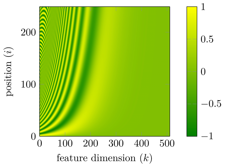
Figure 21: A heat map of the positional embedding model of Eqs. (208) and (209) ($b_{\textrm{model}}=10,000$ and $d_{\textrm{model}}=512$). Consider a position $i$ (i.e., the $i$-th row), then move another position $j$ from $i$ upwards or downwards. Intuitively, when $i$ and $j$ are closer, the corresponding row vectors are more similar. By contrast, when $j$ moves away from $i$, the similarity is not that obvious. This property helps explain the idea behind the positional embedding model: the “distance” between two positions is implicitly modeled by comparing their multi-dimensional representations.

Note that Eqs. (208) and (209) have a useful property that $\mathrm{PE}(i+\mu)$ can be easily expressed by a linear function of $\mathrm{PE}(i)$ for a given offset $\mu$

$$\mathrm{PE}(i+\mu,2k) = \mathrm{PE}(i,2k)\cdot\mathrm{PE}(\mu,2k+1)+$$ (212)

$$\mathrm{PE}(i,2k+1)\cdot\mathrm{PE}(\mu,2k)$$

$$\mathrm{PE}(i+\mu,2k+1) = \mathrm{PE}(i,2k+1)\cdot\mathrm{PE}(\mu,2k+1)+$$ (213)

$$\mathrm{PE}(i,2k)\cdot\mathrm{PE}(\mu,2k)$$

The resulting benefit is that the encoding can somewhat model relative positions. That is, the state at position $i+\mu$ can be described by starting with $i$ and then appending it with the offset $\mu$.

When applying the sinusoidal positional encoding, one way is to concatenate $\mathbf{x}_{i}$ and $\mathrm{PE}(i)$. In Vaswani et al. (2017)’s work, they instead assume $\mathrm{PE}(i)$ to be a vector of the same size as $\mathbf{x}_{i}$ (i.e., $|\mathrm{PE}(i)|=|\mathbf{x}_{i}|=d_{e}$), and add $\mathrm{PE}(i)$ to $\mathbf{x}_{i}$, like this

$$\mathbf{xp}_{i} = \mathbf{x}_{i}+\mathrm{PE}(i)$$ (214)

This sinusoidal addictive model has been the basis of many positional encoding approaches (Dehghani et al., 2018; Likhomanenko et al., 2021; Su et al., 2021).

References

- Adi et al. (2016) Yossi Adi, Einat Kermany, Yonatan Belinkov, Ofer Lavi, and Yoav Goldberg. Fine-grained analysis of sentence embeddings using auxiliary prediction tasks. In Proceedings of International Conference on Learning Representations, 2016.
- Ainslie et al. (2020) Joshua Ainslie, Santiago Ontanon, Chris Alberti, Vaclav Cvicek, Zachary Fisher, Philip Pham, Anirudh Ravula, Sumit Sanghai, Qifan Wang, and Li Yang. Etc: Encoding long and structured inputs in transformers. In Proceedings of the 2020 Conference on Empirical Methods in Natural Language Processing (EMNLP), pages 268–284, 2020.
- Alayrac et al. (2022) Jean-Baptiste Alayrac, Jeff Donahue, Pauline Luc, Antoine Miech, Iain Barr, Yana Hasson, Karel Lenc, Arthur Mensch, Katherine Millican, Malcolm Reynolds, et al. Flamingo: a visual language model for few-shot learning. Advances in Neural Information Processing Systems, 35:23716–23736, 2022.
- Antol et al. (2015) Stanislaw Antol, Aishwarya Agrawal, Jiasen Lu, Margaret Mitchell, Dhruv Batra, C Lawrence Zitnick, and Devi Parikh. Vqa: Visual question answering. In Proceedings of the IEEE international conference on computer vision, pages 2425–2433, 2015.
- Åström and Wittenmark (2013) Karl J Åström and Björn Wittenmark. Computer-controlled systems: theory and design. Courier Corporation, 2013.
- Ba et al. (2016) Jimmy Lei Ba, Jamie Ryan Kiros, and Geoffrey E Hinton. Layer normalization. arXiv preprint arXiv:1607.06450, 2016.
- Bachlechner et al. (2021) Thomas Bachlechner, Bodhisattwa Prasad Majumder, Henry Mao, Gary Cottrell, and Julian McAuley. Rezero is all you need: Fast convergence at large depth. In Proceedings of Uncertainty in Artificial Intelligence, pages 1352–1361. PMLR, 2021.
- Bahdanau et al. (2014) Dzmitry Bahdanau, Kyunghyun Cho, and Yoshua Bengio. Neural machine translation by jointly learning to align and translate. arXiv preprint arXiv:1409.0473, 2014.
- Bai et al. (2021) Jiangang Bai, Yujing Wang, Yiren Chen, Yaming Yang, Jing Bai, Jing Yu, and Yunhai Tong. Syntax-bert: Improving pre-trained transformers with syntax trees. In Proceedings of the 16th Conference of the European Chapter of the Association for Computational Linguistics: Main Volume, pages 3011–3020, 2021.
- Bao et al. (2021) Hangbo Bao, Li Dong, Songhao Piao, and Furu Wei. Beit: Bert pre-training of image transformers. In Proceedings of International Conference on Learning Representations, 2021.
- Barham et al. (2022) Paul Barham, Aakanksha Chowdhery, Jeff Dean, Sanjay Ghemawat, Steven Hand, Daniel Hurt, Michael Isard, Hyeontaek Lim, Ruoming Pang, Sudip Roy, et al. Pathways: Asynchronous distributed dataflow for ml. In Proceedings of Machine Learning and Systems, volume 4, pages 430–449, 2022.
- Belinkov (2022) Yonatan Belinkov. Probing classifiers: Promises, shortcomings, and advances. Computational Linguistics, 48(1):207–219, 2022.
- Bello (2020) Irwan Bello. Lambdanetworks: Modeling long-range interactions without attention. In Proceedings of International Conference on Learning Representations, 2020.
- Beltagy et al. (2020) Iz Beltagy, Matthew E. Peters, and Arman Cohan. Longformer: The long-document transformer. arXiv:2004.05150, 2020.
- Bengio et al. (2015) Emmanuel Bengio, Pierre-Luc Bacon, Joelle Pineau, and Doina Precup. Conditional computation in neural networks for faster models. arXiv preprint arXiv:1511.06297, 2015.
- Bengio et al. (2003) Yoshua Bengio, Réjean Ducharme, Pascal Vincent, and Christian Jauvin. A neural probabilistic language model. Journal of Machine Learning Research, 3:1137–1155, 2003.
- Bengio et al. (2013) Yoshua Bengio, Nicholas Léonard, and Aaron Courville. Estimating or propagating gradients through stochastic neurons for conditional computation. arXiv preprint arXiv:1308.3432, 2013.
- Bhattamishra et al. (2020) Satwik Bhattamishra, Kabir Ahuja, and Navin Goyal. On the ability and limitations of transformers to recognize formal languages. In Proceedings of the 2020 Conference on Empirical Methods in Natural Language Processing (EMNLP), pages 7096–7116, 2020.
- Bommasani et al. (2021) Rishi Bommasani, Drew A. Hudson, Ehsan Adeli, Russ Altman, Simran Arora, Sydney von Arx, Michael S. Bernstein, Jeannette Bohg, Antoine Bosselut, Emma Brunskill, Erik Brynjolfsson, S. Buch, Dallas Card, Rodrigo Castellon, Niladri S. Chatterji, Annie S. Chen, Kathleen A. Creel, Jared Davis, Dora Demszky, Chris Donahue, Moussa Doumbouya, Esin Durmus, Stefano Ermon, John Etchemendy, Kawin Ethayarajh, Li Fei-Fei, Chelsea Finn, Trevor Gale, Lauren E. Gillespie, Karan Goel, Noah D. Goodman, Shelby Grossman, Neel Guha, Tatsunori Hashimoto, Peter Henderson, John Hewitt, Daniel E. Ho, Jenny Hong, Kyle Hsu, Jing Huang, Thomas F. Icard, Saahil Jain, Dan Jurafsky, Pratyusha Kalluri, Siddharth Karamcheti, Geoff Keeling, Fereshte Khani, O. Khattab, Pang Wei Koh, Mark S. Krass, Ranjay Krishna, Rohith Kuditipudi, Ananya Kumar, Faisal Ladhak, Mina Lee, Tony Lee, Jure Leskovec, Isabelle Levent, Xiang Lisa Li, Xuechen Li, Tengyu Ma, Ali Malik, Christopher D. Manning, Suvir P. Mirchandani, Eric Mitchell, Zanele Munyikwa, Suraj Nair, Avanika Narayan, Deepak Narayanan, Benjamin Newman, Allen Nie, Juan Carlos Niebles, Hamed Nilforoshan, J. F. Nyarko, Giray Ogut, Laurel Orr, Isabel Papadimitriou, Joon Sung Park, Chris Piech, Eva Portelance, Christopher Potts, Aditi Raghunathan, Robert Reich, Hongyu Ren, Frieda Rong, Yusuf H. Roohani, Camilo Ruiz, Jack Ryan, Christopher R’e, Dorsa Sadigh, Shiori Sagawa, Keshav Santhanam, Andy Shih, Krishna Parasuram Srinivasan, Alex Tamkin, Rohan Taori, Armin W. Thomas, Florian Tramèr, Rose E. Wang, William Wang, Bohan Wu, Jiajun Wu, Yuhuai Wu, Sang Michael Xie, Michihiro Yasunaga, Jiaxuan You, Matei A. Zaharia, Michael Zhang, Tianyi Zhang, Xikun Zhang, Yuhui Zhang, Lucia Zheng, Kaitlyn Zhou, and Percy Liang. On the opportunities and risks of foundation models. ArXiv, 2021.
- Bondarenko et al. (2021) Yelysei Bondarenko, Markus Nagel, and Tijmen Blankevoort. Understanding and overcoming the challenges of efficient transformer quantization. In Proceedings of the 2021 Conference on Empirical Methods in Natural Language Processing, pages 7947–7969, 2021.
- Brown et al. (2020) Tom Brown, Benjamin Mann, Nick Ryder, Melanie Subbiah, Jared D Kaplan, Prafulla Dhariwal, Arvind Neelakantan, Pranav Shyam, Girish Sastry, Amanda Askell, et al. Language models are few-shot learners. Advances in neural information processing systems, 33:1877–1901, 2020.
- Bubeck et al. (2023) Sébastien Bubeck, Varun Chandrasekaran, Ronen Eldan, Johannes Gehrke, Eric Horvitz, Ece Kamar, Peter Lee, Yin Tat Lee, Yuanzhi Li, Scott Lundberg, et al. Sparks of artificial general intelligence: Early experiments with gpt-4. arXiv preprint arXiv:2303.12712, 2023.
- Burchi and Vielzeuf (2021) Maxime Burchi and Valentin Vielzeuf. Efficient conformer: Progressive downsampling and grouped attention for automatic speech recognition. In Proceedings of 2021 IEEE Automatic Speech Recognition and Understanding Workshop (ASRU), pages 8–15. IEEE, 2021.
- Caron et al. (2021) Mathilde Caron, Hugo Touvron, Ishan Misra, Hervé Jégou, Julien Mairal, Piotr Bojanowski, and Armand Joulin. Emerging properties in self-supervised vision transformers. In Proceedings of the IEEE/CVF international conference on computer vision, pages 9650–9660, 2021.
- Cer et al. (2018) Daniel Cer, Yinfei Yang, Sheng-yi Kong, Nan Hua, Nicole Limtiaco, Rhomni St John, Noah Constant, Mario Guajardo-Cespedes, Steve Yuan, Chris Tar, et al. Universal sentence encoder. arXiv preprint arXiv:1803.11175, 2018.
- Chen et al. (2018a) Kehai Chen, Rui Wang, Masao Utiyama, Eiichiro Sumita, and Tiejun Zhao. Syntax-directed attention for neural machine translation. In Proceedings of the AAAI conference on artificial intelligence, 2018a.
- Chen et al. (2018b) Mia Xu Chen, Orhan Firat, Ankur Bapna, Melvin Johnson, Wolfgang Macherey, George Foster, Llion Jones, Mike Schuster, Noam Shazeer, Niki Parmar, Ashish Vaswani, Jakob Uszkoreit, Lukasz Kaiser, Zhifeng Chen, Yonghui Wu, and Macduff Hughes. The best of both worlds: Combining recent advances in neural machine translation. In Proceedings of the 56th Annual Meeting of the Association for Computational Linguistics (Volume 1: Long Papers), pages 76–86, 2018b.
- Chen et al. (2018c) Ricky TQ Chen, Yulia Rubanova, Jesse Bettencourt, and David K Duvenaud. Neural ordinary differential equations. Advances in neural information processing systems, 31, 2018c.
- Chen et al. (2015) Tianqi Chen, Ian Goodfellow, and Jonathon Shlens. Net2net: Accelerating learning via knowledge transfer. arXiv preprint arXiv:1511.05641, 2015.
- Chiang et al. (2023) David Chiang, Peter Cholak, and Anand Pillay. Tighter bounds on the expressivity of transformer encoders. arXiv preprint arXiv:2301.10743, 2023.
- Child et al. (2019) Rewon Child, Scott Gray, Alec Radford, and Ilya Sutskever. Generating long sequences with sparse transformers. arXiv preprint arXiv:1904.10509, 2019.
- Cho et al. (2021) Jaemin Cho, Jie Lei, Hao Tan, and Mohit Bansal. Unifying vision-and-language tasks via text generation. In International Conference on Machine Learning, pages 1931–1942. PMLR, 2021.
- Choe and Charniak (2016) Do Kook Choe and Eugene Charniak. Parsing as language modeling. In Proceedings of the 2016 Conference on Empirical Methods in Natural Language Processing, pages 2331–2336, 2016.
- Choromanski et al. (2020) Krzysztof Marcin Choromanski, Valerii Likhosherstov, David Dohan, Xingyou Song, Andreea Gane, Tamas Sarlos, Peter Hawkins, Jared Quincy Davis, Afroz Mohiuddin, Lukasz Kaiser, et al. Rethinking attention with performers. In Proceedings of International Conference on Learning Representations, 2020.
- Chowdhery et al. (2022) Aakanksha Chowdhery, Sharan Narang, Jacob Devlin, Maarten Bosma, Gaurav Mishra, Adam Roberts, Paul Barham, Hyung Won Chung, Charles Sutton, Sebastian Gehrmann, et al. Palm: Scaling language modeling with pathways. arXiv preprint arXiv:2204.02311, 2022.
- Clark et al. (2019) Kevin Clark, Urvashi Khandelwal, Omer Levy, and Christopher D Manning. What does bert look at? an analysis of bert’s attention. In Proceedings of the 2019 ACL Workshop BlackboxNLP: Analyzing and Interpreting Neural Networks for NLP, pages 276–286, 2019.
- Conneau et al. (2018) Alexis Conneau, Germán Kruszewski, Guillaume Lample, Loïc Barrault, and Marco Baroni. What you can cram into a single vector: Probing sentence embeddings for linguistic properties. In Proceedings of the 56th Annual Meeting of the Association for Computational Linguistics (Volume 1: Long Papers), pages 2126–2136, 2018.
- Currey and Heafield (2018) Anna Currey and Kenneth Heafield. Multi-source syntactic neural machine translation. In Proceedings of the 2018 Conference on Empirical Methods in Natural Language Processing, pages 2961–2966, 2018.
- Dai et al. (2019) Zihang Dai, Zhilin Yang, Yiming Yang, Jaime G Carbonell, Quoc Le, and Ruslan Salakhutdinov. Transformer-xl: Attentive language models beyond a fixed-length context. In Proceedings of the 57th Annual Meeting of the Association for Computational Linguistics, pages 2978–2988, 2019.
- Dao et al. (2022) Tri Dao, Dan Fu, Stefano Ermon, Atri Rudra, and Christopher Ré. Flashattention: Fast and memory-efficient exact attention with io-awareness. Advances in Neural Information Processing Systems, 35:16344–16359, 2022.
- Dao et al. (2023) Tri Dao, Daniel Haziza, Francisco Massa, and Grigory Sizov. Flash-decoding for long-context inference. https://pytorch.org/blog/flash-decoding/, 2023. Retrieved 2023-10-23.
- Dehghani et al. (2018) Mostafa Dehghani, Stephan Gouws, Oriol Vinyals, Jakob Uszkoreit, and Łukasz Kaiser. Universal transformers. arXiv preprint arXiv:1807.03819, 2018.
- Del Corro et al. (2023) Luciano Del Corro, Allie Del Giorno, Sahaj Agarwal, Bin Yu, Ahmed Awadallah, and Subhabrata Mukherjee. Skipdecode: Autoregressive skip decoding with batching and caching for efficient llm inference. arXiv preprint arXiv:2307.02628, 2023.
- Devlin et al. (2019) Jacob Devlin, Ming-Wei Chang, Kenton Lee, and Kristina Toutanova. Bert: Pre-training of deep bidirectional transformers for language understanding. In Proceedings of the 2019 Conference of the North American Chapter of the Association for Computational Linguistics: Human Language Technologies, Volume 1 (Long and Short Papers), pages 4171–4186, 2019.
- Di Gangi et al. (2019) Mattia Antonino Di Gangi, Matteo Negri, Roldano Cattoni, Roberto Dessi, and Marco Turchi. Enhancing transformer for end-to-end speech-to-text translation. In Proceedings of Machine Translation Summit XVII: Research Track, pages 21–31, 2019.
- Ding et al. (2021) Ming Ding, Zhuoyi Yang, Wenyi Hong, Wendi Zheng, Chang Zhou, Da Yin, Junyang Lin, Xu Zou, Zhou Shao, Hongxia Yang, et al. Cogview: Mastering text-to-image generation via transformers. Advances in Neural Information Processing Systems, 34:19822–19835, 2021.
- Dosovitskiy et al. (2021) Alexey Dosovitskiy, Lucas Beyer, Alexander Kolesnikov, Dirk Weissenborn, Xiaohua Zhai, Thomas Unterthiner, Mostafa Dehghani, Matthias Minderer, Georg Heigold, Sylvain Gelly, et al. An image is worth 16x16 words: Transformers for image recognition at scale. In Proceedings of ICLR 2021, 2021.
- Dufter et al. (2022) Philipp Dufter, Martin Schmitt, and Hinrich Schütze. Position information in transformers: An overview. Computational Linguistics, 48(3):733–763, 2022.
- Ee (2017) Weinan Ee. A proposal on machine learning via dynamical systems. Communications in Mathematics and Statistics, 5:1–11, 02 2017.
- Elbayad et al. (2020) Maha Elbayad, Jiatao Gu, Edouard Grave, and Michael Auli. Depth-adaptive transformer. In Proceedings of International Conference on Learning Representations, 2020.
- Elsken et al. (2019) Thomas Elsken, Jan Hendrik Metzen, and Frank Hutter. Neural architecture search: A survey. The Journal of Machine Learning Research, 20(1):1997–2017, 2019.
- Fan et al. (2021) Haoqi Fan, Bo Xiong, Karttikeya Mangalam, Yanghao Li, Zhicheng Yan, Jitendra Malik, and Christoph Feichtenhofer. Multiscale vision transformers. In Proceedings of the IEEE/CVF International Conference on Computer Vision, pages 6824–6835, 2021.
- Fan et al. (2020) Yang Fan, Shufang Xie, Yingce Xia, Lijun Wu, Tao Qin, Xiang-Yang Li, and Tie-Yan Liu. Multi-branch attentive transformer. arXiv preprint arXiv:2006.10270, 2020.
- Fedus et al. (2022a) William Fedus, Jeff Dean, and Barret Zoph. A review of sparse expert models in deep learning. arXiv preprint arXiv:2209.01667, 2022a.
- Fedus et al. (2022b) William Fedus, Barret Zoph, and Noam Shazeer. Switch transformers: Scaling to trillion parameter models with simple and efficient sparsity. The Journal of Machine Learning Research, 23(1):5232–5270, 2022b.
- Fu et al. (2022) Daniel Y Fu, Tri Dao, Khaled Kamal Saab, Armin W Thomas, Atri Rudra, and Christopher Re. Hungry hungry hippos: Towards language modeling with state space models. In Proceedings of The Eleventh International Conference on Learning Representations, 2022.
- Gehring et al. (2017) Jonas Gehring, Michael Auli, David Grangier, Denis Yarats, and Yann N Dauphin. Convolutional sequence to sequence learning. In International conference on machine learning, pages 1243–1252. PMLR, 2017.
- Gholami et al. (2022) Amir Gholami, Sehoon Kim, Zhen Dong, Zhewei Yao, Michael W Mahoney, and Kurt Keutzer. A survey of quantization methods for efficient neural network inference. In Low-Power Computer Vision, pages 291–326. Chapman and Hall/CRC, 2022.
- Glorot and Bengio (2010) Xavier Glorot and Yoshua Bengio. Understanding the difficulty of training deep feedforward neural networks. In Proceedings of the thirteenth international conference on artificial intelligence and statistics, pages 249–256. JMLR Workshop and Conference Proceedings, 2010.
- Gomez et al. (2017) Aidan N Gomez, Mengye Ren, Raquel Urtasun, and Roger B Grosse. The reversible residual network: Backpropagation without storing activations. Advances in neural information processing systems, 30, 2017.
- Gou et al. (2021) Jianping Gou, Baosheng Yu, Stephen J Maybank, and Dacheng Tao. Knowledge distillation: A survey. International Journal of Computer Vision, 129:1789–1819, 2021.
- Gray (1998) Robert M. Gray. Quantization. IEEE transactions on information theory, 44(6):2325–2383, 1998.
- Gu et al. (2021) Albert Gu, Karan Goel, and Christopher Ré. Efficiently modeling long sequences with structured state spaces. In Proceedings of International Conference on Learning Representations, 2021.
- Gu et al. (2022a) Albert Gu, Karan Goel, Ankit Gupta, and Christopher Ré. On the parameterization and initialization of diagonal state space models. Advances in Neural Information Processing Systems, 35:35971–35983, 2022a.
- Gu et al. (2022b) Albert Gu, Karan Goel, Khaled Saab, and Chris Ré. Structured state spaces: Combining continuous-time, recurrent, and convolutional models. https://hazyresearch.stanford.edu/blog/2022-01-14-s4-3, 2022b. Retrieved 2022-01-14.
- Gulati et al. (2020) Anmol Gulati, James Qin, Chung-Cheng Chiu, Niki Parmar, Yu Zhang, Jiahui Yu, Wei Han, Shibo Wang, Zhengdong Zhang, Yonghui Wu, and Ruoming Pang. Conformer: Convolution-augmented transformer for speech recognition. Proceedings of Interspeech 2020, pages 5036–5040, 2020.
- Guo et al. (2020) Qipeng Guo, Xipeng Qiu, Pengfei Liu, Xiangyang Xue, and Zheng Zhang. Multi-scale self-attention for text classification. In Proceedings of the AAAI Conference on Artificial Intelligence, volume 34, pages 7847–7854, 2020.
- Gupta et al. (2004) Madan Gupta, Liang Jin, and Noriyasu Homma. Static and dynamic neural networks: from fundamentals to advanced theory. John Wiley & Sons, 2004.
- Guu et al. (2020) Kelvin Guu, Kenton Lee, Zora Tung, Panupong Pasupat, and Mingwei Chang. Retrieval augmented language model pre-training. In Proceedings of International conference on machine learning, pages 3929–3938. PMLR, 2020.
- Haber and Ruthotto (2017) Eldad Haber and Lars Ruthotto. Stable architectures for deep neural networks. Inverse problems, 34(1):014004, 2017.
- Hahn (2020) Michael Hahn. Theoretical limitations of self-attention in neural sequence models. Transactions of the Association for Computational Linguistics, 8:156–171, 2020.
- Han et al. (2022) Kai Han, Yunhe Wang, Hanting Chen, Xinghao Chen, Jianyuan Guo, Zhenhua Liu, Yehui Tang, An Xiao, Chunjing Xu, Yixing Xu, et al. A survey on vision transformer. IEEE transactions on pattern analysis and machine intelligence, 45(1):87–110, 2022.
- Han et al. (2020) Wei Han, Zhengdong Zhang, Yu Zhang, Jiahui Yu, Chung-Cheng Chiu, James Qin, Anmol Gulati, Ruoming Pang, and Yonghui Wu. Contextnet: Improving convolutional neural networks for automatic speech recognition with global context. In Proceedings of Interspeech 2020, pages 3610–3614, 2020.
- Han et al. (2021) Yizeng Han, Gao Huang, Shiji Song, Le Yang, Honghui Wang, and Yulin Wang. Dynamic neural networks: A survey. IEEE Transactions on Pattern Analysis and Machine Intelligence, 44(11):7436–7456, 2021.
- Hao et al. (2019) Jie Hao, Xing Wang, Shuming Shi, Jinfeng Zhang, and Zhaopeng Tu. Multi-granularity self-attention for neural machine translation. In Proceedings of the 2019 Conference on Empirical Methods in Natural Language Processing and the 9th International Joint Conference on Natural Language Processing (EMNLP-IJCNLP), pages 887–897, 2019.
- Hao et al. (2022) Yiding Hao, Dana Angluin, and Robert Frank. Formal language recognition by hard attention transformers: Perspectives from circuit complexity. Transactions of the Association for Computational Linguistics, 10:800–810, 2022.
- He et al. (2016a) Kaiming He, Xiangyu Zhang, Shaoqing Ren, and Jian Sun. Deep residual learning for image recognition. In Proceedings of the IEEE conference on computer vision and pattern recognition, pages 770–778, 2016a.
- He et al. (2016b) Kaiming He, Xiangyu Zhang, Shaoqing Ren, and Jian Sun. Identity mappings in deep residual networks. In Proceedings of ECCV 2016, pages 630–645, 2016b.
- He et al. (2022) Kaiming He, Xinlei Chen, Saining Xie, Yanghao Li, Piotr Dollár, and Ross Girshick. Masked autoencoders are scalable vision learners. In Proceedings of the IEEE/CVF Conference on Computer Vision and Pattern Recognition, pages 16000–16009, 2022.
- He et al. (2021) Pengcheng He, Xiaodong Liu, Jianfeng Gao, and Weizhu Chen. Deberta: Decoding-enhanced bert with disentangled attention. In Proceedings of International Conference on Learning Representations, 2021.
- Heafield et al. (2021) Kenneth Heafield, Qianqian Zhu, and Roman Grundkiewicz. Findings of the WMT 2021 shared task on efficient translation. In Proceedings of the Sixth Conference on Machine Translation, pages 639–651, 2021.
- Hestness et al. (2017) Joel Hestness, Sharan Narang, Newsha Ardalani, Gregory Diamos, Heewoo Jun, Hassan Kianinejad, Md Mostofa Ali Patwary, Yang Yang, and Yanqi Zhou. Deep learning scaling is predictable, empirically. arXiv preprint arXiv:1712.00409, 2017.
- Hewitt and Liang (2019) John Hewitt and Percy Liang. Designing and interpreting probes with control tasks. In Proceedings of the 2019 Conference on Empirical Methods in Natural Language Processing and the 9th International Joint Conference on Natural Language Processing (EMNLP-IJCNLP), pages 2733–2743, 2019.
- Hill et al. (2016) Felix Hill, Kyunghyun Cho, and Anna Korhonen. Learning distributed representations of sentences from unlabelled data. In Proceedings of the 2016 Conference of the North American Chapter of the Association for Computational Linguistics: Human Language Technologies, pages 1367–1377, 2016.
- Hinton et al. (2015) Geoffrey Hinton, Oriol Vinyals, and Jeff Dean. Distilling the knowledge in a neural network. arXiv preprint arXiv:1503.02531, 2015.
- Hou et al. (2020) Lu Hou, Zhiqi Huang, Lifeng Shang, Xin Jiang, Xiao Chen, and Qun Liu. Dynabert: Dynamic bert with adaptive width and depth. Advances in Neural Information Processing Systems, 33:9782–9793, 2020.
- Howard et al. (2019) Andrew Howard, Mark Sandler, Grace Chu, Liang-Chieh Chen, Bo Chen, Mingxing Tan, Weijun Wang, Yukun Zhu, Ruoming Pang, Vijay Vasudevan, et al. Searching for mobilenetv3. In Proceedings of the IEEE/CVF international conference on computer vision, pages 1314–1324, 2019.
- Hu et al. (2021) Chi Hu, Chenglong Wang, Xiangnan Ma, Xia Meng, Yinqiao Li, Tong Xiao, Jingbo Zhu, and Changliang Li. Ranknas: Efficient neural architecture search by pairwise ranking. In Proceedings of the 2021 Conference on Empirical Methods in Natural Language Processing, pages 2469–2480, 2021.
- Huang et al. (2018) Cheng-Zhi Anna Huang, Ashish Vaswani, Jakob Uszkoreit, Ian Simon, Curtis Hawthorne, Noam Shazeer, Andrew M Dai, Matthew D Hoffman, Monica Dinculescu, and Douglas Eck. Music transformer: Generating music with long-term structure. In Proceedings of International Conference on Learning Representations, 2018.
- Huang et al. (2016) Gao Huang, Yu Sun, Zhuang Liu, Daniel Sedra, and Kilian Q Weinberger. Deep networks with stochastic depth. In Proceedings of the 14th European Conference, pages 646–661. Springer, 2016.
- Huang et al. (2017) Gao Huang, Zhuang Liu, Laurens Van Der Maaten, and Kilian Q Weinberger. Densely connected convolutional networks. In Proceedings of the IEEE conference on computer vision and pattern recognition, pages 4700–4708, 2017.
- Huang et al. (2020) Zhiheng Huang, Davis Liang, Peng Xu, and Bing Xiang. Improve transformer models with better relative position embeddings. In Findings of the Association for Computational Linguistics: EMNLP 2020, pages 3327–3335, 2020.
- Ivanov et al. (2021) Andrei Ivanov, Nikoli Dryden, Tal Ben-Nun, Shigang Li, and Torsten Hoefler. Data movement is all you need: A case study on optimizing transformers. In Proceedings of Machine Learning and Systems, volume 3, pages 711–732, 2021.
- Jacob et al. (2018) Benoit Jacob, Skirmantas Kligys, Bo Chen, Menglong Zhu, Matthew Tang, Andrew Howard, Hartwig Adam, and Dmitry Kalenichenko. Quantization and training of neural networks for efficient integer-arithmetic-only inference. In Proceedings of the IEEE conference on computer vision and pattern recognition, pages 2704–2713, 2018.
- Jaegle et al. (2021) Andrew Jaegle, Sebastian Borgeaud, Jean-Baptiste Alayrac, Carl Doersch, Catalin Ionescu, David Ding, Skanda Koppula, Daniel Zoran, Andrew Brock, Evan Shelhamer, et al. Perceiver io: A general architecture for structured inputs & outputs. In Proceedings of International Conference on Learning Representations, 2021.
- Kaplan et al. (2020) Jared Kaplan, Sam McCandlish, Tom Henighan, Tom B Brown, Benjamin Chess, Rewon Child, Scott Gray, Alec Radford, Jeffrey Wu, and Dario Amodei. Scaling laws for neural language models. arXiv preprint arXiv:2001.08361, 2020.
- Katharopoulos et al. (2020) Angelos Katharopoulos, Apoorv Vyas, Nikolaos Pappas, and François Fleuret. Transformers are rnns: Fast autoregressive transformers with linear attention. In International conference on machine learning, pages 5156–5165. PMLR, 2020.
- Kernes (2021) Jonathan Kernes. Master positional encoding: Part i, 05 2021. URL https://towardsdatascience.com/master-positional-encoding-part-i-63c05d90a0c3.
- Kidger (2022) Patrick Kidger. On neural differential equations. arXiv preprint arXiv:2202.02435, 2022.
- Kim and Cho (2021) Gyuwan Kim and Kyunghyun Cho. Length-adaptive transformer: Train once with length drop, use anytime with search. In Proceedings of the 59th Annual Meeting of the Association for Computational Linguistics and the 11th International Joint Conference on Natural Language Processing (Volume 1: Long Papers), pages 6501–6511, 2021.
- Kim et al. (2019) Najoung Kim, Roma Patel, Adam Poliak, Patrick Xia, Alex Wang, Tom McCoy, Ian Tenney, Alexis Ross, Tal Linzen, Benjamin Van Durme, et al. Probing what different nlp tasks teach machines about function word comprehension. In Proceedings of the Eighth Joint Conference on Lexical and Computational Semantics (* SEM 2019), pages 235–249, 2019.
- Kim et al. (2023) Sehoon Kim, Coleman Hooper, Thanakul Wattanawong, Minwoo Kang, Ruohan Yan, Hasan Genc, Grace Dinh, Qijing Huang, Kurt Keutzer, Michael W Mahoney, et al. Full stack optimization of transformer inference: a survey. arXiv preprint arXiv:2302.14017, 2023.
- Kim et al. (2021) Wonjae Kim, Bokyung Son, and Ildoo Kim. Vilt: Vision-and-language transformer without convolution or region supervision. In Proceedings of International Conference on Machine Learning, pages 5583–5594. PMLR, 2021.
- Kim and Rush (2016) Yoon Kim and Alexander M Rush. Sequence-level knowledge distillation. In Proceedings of the 2016 Conference on Empirical Methods in Natural Language Processing, pages 1317–1327, 2016.
- Kim and Awadalla (2020) Young Jin Kim and Hany Hassan Awadalla. Fastformers: Highly efficient transformer models for natural language understanding. In Proceedings of SustaiNLP: Workshop on Simple and Efficient Natural Language Processing, pages 149–158, 2020.
- Kingma and Ba (2014) Diederik P Kingma and Jimmy Ba. Adam: A method for stochastic optimization. arXiv preprint arXiv:1412.6980, 2014.
- Kitaev et al. (2020) Nikita Kitaev, Lukasz Kaiser, and Anselm Levskaya. Reformer: The efficient transformer. In Proceedings of International Conference on Learning Representations, 2020.
- Kudo (2018) Taku Kudo. Subword regularization: Improving neural network translation models with multiple subword candidates. In Proceedings of the 56th Annual Meeting of the Association for Computational Linguistics (Volume 1: Long Papers), pages 66–75, 2018.
- Kwon et al. (2023) Woosuk Kwon, Zhuohan Li, Siyuan Zhuang, Ying Sheng, Lianmin Zheng, Cody Hao Yu, Joseph E Gonzalez, Hao Zhang, and Ion Stoica. Efficient memory management for large language model serving with pagedattention. arXiv preprint arXiv:2309.06180, 2023.
- Lagunas et al. (2021) François Lagunas, Ella Charlaix, Victor Sanh, and Alexander M Rush. Block pruning for faster transformers. In Proceedings of the 2021 Conference on Empirical Methods in Natural Language Processing, pages 10619–10629, 2021.
- Lample et al. (2019) Guillaume Lample, Alexandre Sablayrolles, Marc’Aurelio Ranzato, Ludovic Denoyer, and Hervé Jégou. Large memory layers with product keys. Advances in Neural Information Processing Systems, 32, 2019.
- Lepikhin et al. (2021) Dmitry Lepikhin, HyoukJoong Lee, Yuanzhong Xu, Dehao Chen, Orhan Firat, Yanping Huang, Maxim Krikun, Noam Shazeer, and Zhifeng Chen. Gshard: Scaling giant models with conditional computation and automatic sharding. In Proceedings of International Conference on Learning Representations, 2021.
- Leviathan et al. (2023) Yaniv Leviathan, Matan Kalman, and Yossi Matias. Fast inference from transformers via speculative decoding. In Proceedings of International Conference on Machine Learning, pages 19274–19286. PMLR, 2023.
- Lewis et al. (2020) Patrick Lewis, Ethan Perez, Aleksandra Piktus, Fabio Petroni, Vladimir Karpukhin, Naman Goyal, Heinrich Küttler, Mike Lewis, Wen-tau Yih, Tim Rocktäschel, et al. Retrieval-augmented generation for knowledge-intensive nlp tasks. Advances in Neural Information Processing Systems, 33:9459–9474, 2020.
- Li et al. (2020a) Bei Li, Hui Liu, Ziyang Wang, Yufan Jiang, Tong Xiao, Jingbo Zhu, Tongran Liu, and Changliang Li. Does multi-encoder help? a case study on context-aware neural machine translation. In Proceedings of the 58th Annual Meeting of the Association for Computational Linguistics, pages 3512–3518, 2020a.
- Li et al. (2020b) Bei Li, Ziyang Wang, Hui Liu, Yufan Jiang, Quan Du, Tong Xiao, Huizhen Wang, and Jingbo Zhu. Shallow-to-deep training for neural machine translation. In Proceedings of the 2020 Conference on Empirical Methods in Natural Language Processing (EMNLP), pages 995–1005, 2020b.
- Li et al. (2021) Bei Li, Ziyang Wang, Hui Liu, Quan Du, Tong Xiao, Chunliang Zhang, and Jingbo Zhu. Learning light-weight translation models from deep transformer. In Proceedings of the AAAI Conference on Artificial Intelligence, volume 35, pages 13217–13225, 2021.
- Li et al. (2022a) Bei Li, Quan Du, Tao Zhou, Yi Jing, Shuhan Zhou, Xin Zeng, Tong Xiao, Jingbo Zhu, Xuebo Liu, and Min Zhang. Ode transformer: An ordinary differential equation-inspired model for sequence generation. In Proceedings of the 60th Annual Meeting of the Association for Computational Linguistics (Volume 1: Long Papers), pages 8335–8351, 2022a.
- Li et al. (2022b) Bei Li, Tong Zheng, Yi Jing, Chengbo Jiao, Tong Xiao, and Jingbo Zhu. Learning multiscale transformer models for sequence generation. In International Conference on Machine Learning, pages 13225–13241. PMLR, 2022b.
- Li et al. (2022c) Hongkang Li, Meng Wang, Sijia Liu, and Pin-Yu Chen. A theoretical understanding of shallow vision transformers: Learning, generalization, and sample complexity. In The Eleventh International Conference on Learning Representations, 2022c.
- Li et al. (2017) Junhui Li, Deyi Xiong, Zhaopeng Tu, Muhua Zhu, Min Zhang, and Guodong Zhou. Modeling source syntax for neural machine translation. In Proceedings of the 55th Annual Meeting of the Association for Computational Linguistics (Volume 1: Long Papers), pages 688–697, 2017.
- Li et al. (2022d) Junnan Li, Dongxu Li, Caiming Xiong, and Steven Hoi. Blip: Bootstrapping language-image pre-training for unified vision-language understanding and generation. In International Conference on Machine Learning, pages 12888–12900. PMLR, 2022d.
- Li et al. (2022e) Yanghao Li, Chao-Yuan Wu, Haoqi Fan, Karttikeya Mangalam, Bo Xiong, Jitendra Malik, and Christoph Feichtenhofer. Mvitv2: Improved multiscale vision transformers for classification and detection. In Proceedings of the IEEE/CVF Conference on Computer Vision and Pattern Recognition, pages 4804–4814, 2022e.
- Liao et al. (2021) Kaiyuan Liao, Yi Zhang, Xuancheng Ren, Qi Su, Xu Sun, and Bin He. A global past-future early exit method for accelerating inference of pre-trained language models. In Proceedings of the 2021 Conference of the North American Chapter of the Association for Computational Linguistics: Human Language Technologies, pages 2013–2023, 2021.
- Likhomanenko et al. (2021) Tatiana Likhomanenko, Qiantong Xu, Gabriel Synnaeve, Ronan Collobert, and Alex Rogozhnikov. Cape: Encoding relative positions with continuous augmented positional embeddings. Advances in Neural Information Processing Systems, 34:16079–16092, 2021.
- Lin et al. (2022a) Tianyang Lin, Yuxin Wang, Xiangyang Liu, and Xipeng Qiu. A survey of transformers. AI Open, 2022a.
- Lin et al. (2022b) Ye Lin, Shuhan Zhou, Yanyang Li, Anxiang Ma, Tong Xiao, and Jingbo Zhu. Multi-path transformer is better: A case study on neural machine translation. In Findings of the Association for Computational Linguistics: EMNLP 2022, pages 5646–5656, 2022b.
- Liu et al. (2020a) Fenglin Liu, Xuancheng Ren, Zhiyuan Zhang, Xu Sun, and Yuexian Zou. Rethinking skip connection with layer normalization. In Proceedings of the 28th international conference on computational linguistics, pages 3586–3598, 2020a.
- Liu et al. (2023a) Haotian Liu, Chunyuan Li, Qingyang Wu, and Yong Jae Lee. Visual instruction tuning. arXiv preprint arXiv:2304.08485, 2023a.
- Liu et al. (2020b) Liyuan Liu, Xiaodong Liu, Jianfeng Gao, Weizhu Chen, and Jiawei Han. Understanding the difficulty of training transformers. In Proceedings of the 2020 Conference on Empirical Methods in Natural Language Processing (EMNLP), pages 5747–5763, 2020b.
- Liu et al. (2018) Peter J Liu, Mohammad Saleh, Etienne Pot, Ben Goodrich, Ryan Sepassi, Lukasz Kaiser, and Noam Shazeer. Generating wikipedia by summarizing long sequences. In Proceedings of International Conference on Learning Representations, 2018.
- Liu et al. (2023b) Yang Liu, Yao Zhang, Yixin Wang, Feng Hou, Jin Yuan, Jiang Tian, Yang Zhang, Zhongchao Shi, Jianping Fan, and Zhiqiang He. A survey of visual transformers. IEEE Transactions on Neural Networks and Learning Systems, 2023b.
- Liu et al. (2020c) Yuchen Liu, Junnan Zhu, Jiajun Zhang, and Chengqing Zong. Bridging the modality gap for speech-to-text translation. arXiv preprint arXiv:2010.14920, 2020c.
- Luong et al. (2015) Minh-Thang Luong, Hieu Pham, and Christopher D Manning. Effective approaches to attention-based neural machine translation. In Proceedings of the 2015 Conference on Empirical Methods in Natural Language Processing, pages 1412–1421, 2015.
- Manning et al. (2020) Christopher D Manning, Kevin Clark, John Hewitt, Urvashi Khandelwal, and Omer Levy. Emergent linguistic structure in artificial neural networks trained by self-supervision. Proceedings of the National Academy of Sciences, 117(48):30046–30054, 2020.
- Martins et al. (2022) Pedro Henrique Martins, Zita Marinho, and André FT Martins. ∞-former: Infinite memory transformer-former: Infinite memory transformer. In Proceedings of the 60th Annual Meeting of the Association for Computational Linguistics (Volume 1: Long Papers), pages 5468–5485, 2022.
- Masoudnia and Ebrahimpour (2014) Saeed Masoudnia and Reza Ebrahimpour. Mixture of experts: a literature survey. The Artificial Intelligence Review, 42(2):275, 2014.
- McCarley et al. (2019) JS McCarley, Rishav Chakravarti, and Avirup Sil. Structured pruning of a bert-based question answering model. arXiv preprint arXiv:1910.06360, 2019.
- Merrill et al. (2022) William Merrill, Ashish Sabharwal, and Noah A Smith. Saturated transformers are constant-depth threshold circuits. Transactions of the Association for Computational Linguistics, 10:843–856, 2022.
- Michel et al. (2019) Paul Michel, Omer Levy, and Graham Neubig. Are sixteen heads really better than one? Advances in neural information processing systems, 32, 2019.
- Mikolov et al. (2013) Tomas Mikolov, Ilya Sutskever, Kai Chen, Greg Corrado, and Jeffrey Dean. Distributed representations of words and phrases and their compositionality. In Proceedings of the 26th International Conference on Neural Information Processing Systems - Volume 2, page 3111–3119, 2013.
- Nagel et al. (2021) Markus Nagel, Marios Fournarakis, Rana Ali Amjad, Yelysei Bondarenko, Mart Van Baalen, and Tijmen Blankevoort. A white paper on neural network quantization. arXiv preprint arXiv:2106.08295, 2021.
- Oppenheim and Schafer (1975) Alan V Oppenheim and Ronald W Schafer. Digital signal processing(book). Prentice-Hall, 1975.
- Orvieto et al. (2023) Antonio Orvieto, Samuel L Smith, Albert Gu, Anushan Fernando, Caglar Gulcehre, Razvan Pascanu, and Soham De. Resurrecting recurrent neural networks for long sequences. arXiv preprint arXiv:2303.06349, 2023.
- Ouyang et al. (2022) Long Ouyang, Jeffrey Wu, Xu Jiang, Diogo Almeida, Carroll Wainwright, Pamela Mishkin, Chong Zhang, Sandhini Agarwal, Katarina Slama, Alex Ray, et al. Training language models to follow instructions with human feedback. Advances in Neural Information Processing Systems, 35:27730–27744, 2022.
- Park et al. (2019) Wonpyo Park, Dongju Kim, Yan Lu, and Minsu Cho. Relational knowledge distillation. In Proceedings of the IEEE/CVF conference on computer vision and pattern recognition, pages 3967–3976, 2019.
- Parmar et al. (2018) Niki Parmar, Ashish Vaswani, Jakob Uszkoreit, Lukasz Kaiser, Noam Shazeer, Alexander Ku, and Dustin Tran. Image transformer. In International conference on machine learning, pages 4055–4064. PMLR, 2018.
- Peng et al. (2019) Baoyun Peng, Xiao Jin, Jiaheng Liu, Dongsheng Li, Yichao Wu, Yu Liu, Shunfeng Zhou, and Zhaoning Zhang. Correlation congruence for knowledge distillation. In Proceedings of the IEEE/CVF International Conference on Computer Vision, pages 5007–5016, 2019.
- Peng et al. (2023) Bo Peng, Eric Alcaide, Quentin Anthony, Alon Albalak, Samuel Arcadinho, Huanqi Cao, Xin Cheng, Michael Chung, Matteo Grella, Kranthi Kiran GV, et al. Rwkv: Reinventing rnns for the transformer era. arXiv preprint arXiv:2305.13048, 2023.
- Peng et al. (2021) H Peng, N Pappas, D Yogatama, R Schwartz, N Smith, and L Kong. Random feature attention. In Proceedings of International Conference on Learning Representations (ICLR 2021), 2021.
- Pérez et al. (2018) Jorge Pérez, Javier Marinković, and Pablo Barceló. On the turing completeness of modern neural network architectures. In Proceedings of International Conference on Learning Representations, 2018.
- Petroni et al. (2019) Fabio Petroni, Tim Rocktäschel, Sebastian Riedel, Patrick Lewis, Anton Bakhtin, Yuxiang Wu, and Alexander Miller. Language models as knowledge bases? In Proceedings of the 2019 Conference on Empirical Methods in Natural Language Processing and the 9th International Joint Conference on Natural Language Processing (EMNLP-IJCNLP), pages 2463–2473, 2019.
- Pham et al. (2019) Ngoc-Quan Pham, Thai-Son Nguyen, Jan Niehues, Markus Müller, Sebastian Stüker, and Alexander Waibel. Very deep self-attention networks for end-to-end speech recognition. arXiv preprint arXiv:1904.13377, 2019.
- Pires et al. (2023) Telmo Pessoa Pires, António V Lopes, Yannick Assogba, and Hendra Setiawan. One wide feedforward is all you need. arXiv preprint arXiv:2309.01826, 2023.
- Pope et al. (2023) Reiner Pope, Sholto Douglas, Aakanksha Chowdhery, Jacob Devlin, James Bradbury, Jonathan Heek, Kefan Xiao, Shivani Agrawal, and Jeff Dean. Efficiently scaling transformer inference. In Proceedings of Machine Learning and Systems, 2023.
- Press et al. (2021) Ofir Press, Noah Smith, and Mike Lewis. Train short, test long: Attention with linear biases enables input length extrapolation. In Proceedings of International Conference on Learning Representations, 2021.
- Provilkov et al. (2020) Ivan Provilkov, Dmitrii Emelianenko, and Elena Voita. Bpe-dropout: Simple and effective subword regularization. In Proceedings of the 58th Annual Meeting of the Association for Computational Linguistics, pages 1882–1892, 2020.
- Qiu et al. (2020) Jiezhong Qiu, Hao Ma, Omer Levy, Wen-tau Yih, Sinong Wang, and Jie Tang. Blockwise self-attention for long document understanding. In Findings of the Association for Computational Linguistics: EMNLP 2020, pages 2555–2565, 2020.
- Rabiner and Gold (1975) Lawrence R Rabiner and Bernard Gold. Theory and application of digital signal processing. Prentice-Hall, 1975.
- Rae et al. (2019) Jack W Rae, Anna Potapenko, Siddhant M Jayakumar, Chloe Hillier, and Timothy P Lillicrap. Compressive transformers for long-range sequence modelling. In Proceedings of International Conference on Learning Representations, 2019.
- Raffel et al. (2020) Colin Raffel, Noam Shazeer, Adam Roberts, Katherine Lee, Sharan Narang, Michael Matena, Yanqi Zhou, Wei Li, Peter J Liu, et al. Exploring the limits of transfer learning with a unified text-to-text transformer. Journal of Machine Learning Research, 21(140):1–67, 2020.
- Reimers and Gurevych (2019) Nils Reimers and Iryna Gurevych. Sentence-bert: Sentence embeddings using siamese bert-networks. In Proceedings of the 2019 Conference on Empirical Methods in Natural Language Processing and the 9th International Joint Conference on Natural Language Processing (EMNLP-IJCNLP), pages 3982–3992, 2019.
- Romero et al. (2014) Adriana Romero, Nicolas Ballas, Samira Ebrahimi Kahou, Antoine Chassang, Carlo Gatta, and Yoshua Bengio. Fitnets: Hints for thin deep nets. arXiv preprint arXiv:1412.6550, 2014.
- Roy et al. (2021) Aurko Roy, Mohammad Saffar, Ashish Vaswani, and David Grangier. Efficient content-based sparse attention with routing transformers. Transactions of the Association for Computational Linguistics, 9:53–68, 2021.
- Santacroce et al. (2023) Michael Santacroce, Zixin Wen, Yelong Shen, and Yuanzhi Li. What matters in the structured pruning of generative language models? arXiv preprint arXiv:2302.03773, 2023.
- Schlag et al. (2021) Imanol Schlag, Kazuki Irie, and Jürgen Schmidhuber. Linear transformers are secretly fast weight programmers. In Proceedings of International Conference on Machine Learning, pages 9355–9366. PMLR, 2021.
- Schuster et al. (2022) Tal Schuster, Adam Fisch, Jai Gupta, Mostafa Dehghani, Dara Bahri, Vinh Tran, Yi Tay, and Donald Metzler. Confident adaptive language modeling. Advances in Neural Information Processing Systems, 35:17456–17472, 2022.
- Schwartz et al. (2020) Roy Schwartz, Gabriel Stanovsky, Swabha Swayamdipta, Jesse Dodge, and Noah A Smith. The right tool for the job: Matching model and instance complexities. In Proceedings of the 58th Annual Meeting of the Association for Computational Linguistics, pages 6640–6651, 2020.
- See (2018) Abigail See. Deep learning, structure and innate priors: A discussion between yann lecun and christopher manning, 02 2018. URL http://www.abigailsee.com/2018/02/21/deep-learning-structure-and-innate-priors.html.
- Sennrich et al. (2016) Rico Sennrich, Barry Haddow, and Alexandra Birch. Neural machine translation of rare words with subword units. In Proceedings of the 54th Annual Meeting of the Association for Computational Linguistics (Volume 1: Long Papers), pages 1715–1725, 2016.
- Shaw et al. (2018) Peter Shaw, Jakob Uszkoreit, and Ashish Vaswani. Self-attention with relative position representations. In Proceedings of the 2018 Conference of the North American Chapter of the Association for Computational Linguistics: Human Language Technologies, Volume 2 (Short Papers), pages 464–468, 2018.
- Shazeer (2019) Noam Shazeer. Fast transformer decoding: One write-head is all you need. arXiv preprint arXiv:1911.02150, 2019.
- Shazeer et al. (2017) Noam Shazeer, Azalia Mirhoseini, Krzysztof Maziarz, Andy Davis, Quoc Le, Geoffrey Hinton, and Jeff Dean. Outrageously large neural networks: The sparsely-gated mixture-of-experts layer. In Proceedings of International Conference on Learning Representations, 2017.
- Shen et al. (2020) Dinghan Shen, Mingzhi Zheng, Yelong Shen, Yanru Qu, and Weizhu Chen. A simple but tough-to-beat data augmentation approach for natural language understanding and generation. arXiv preprint arXiv:2009.13818, 2020.
- Shi et al. (2016) Xing Shi, Inkit Padhi, and Kevin Knight. Does string-based neural mt learn source syntax? In Proceedings of the 2016 conference on empirical methods in natural language processing, pages 1526–1534, 2016.
- Skorski et al. (2021) Maciej Skorski, Alessandro Temperoni, and Martin Theobald. Revisiting weight initialization of deep neural networks. In Asian Conference on Machine Learning, pages 1192–1207. PMLR, 2021.
- So et al. (2019) David So, Quoc Le, and Chen Liang. The evolved transformer. In Proceedings of International conference on machine learning, pages 5877–5886. PMLR, 2019.
- Sperber et al. (2018) Matthias Sperber, Jan Niehues, Graham Neubig, Sebastian Stüker, and Alex Waibel. Self-attentional acoustic models. In Proceedings of Interspeech 2018, pages 3723–3727, 2018.
- Srivastava et al. (2015) Rupesh Kumar Srivastava, Klaus Greff, and Jürgen Schmidhuber. Highway networks. arXiv preprint arXiv:1505.00387, 2015.
- Stock et al. (2021) Pierre Stock, Angela Fan, Benjamin Graham, Edouard Grave, Rémi Gribonval, Herve Jegou, and Armand Joulin. Training with quantization noise for extreme model compression. In Proceedings of International Conference on Learning Representations, 2021.
- Strubell et al. (2018) Emma Strubell, Patrick Verga, Daniel Andor, David Weiss, and Andrew McCallum. Linguistically-informed self-attention for semantic role labeling. In Proceedings of the 2018 Conference on Empirical Methods in Natural Language Processing, pages 5027–5038, 2018.
- Su et al. (2021) Jianlin Su, Yu Lu, Shengfeng Pan, Bo Wen, and Yunfeng Liu. Roformer: Enhanced transformer with rotary position embedding. arXiv preprint arXiv:2104.09864, 2021.
- Sukhbaatar et al. (2015) Sainbayar Sukhbaatar, Jason Weston, Rob Fergus, et al. End-to-end memory networks. Advances in neural information processing systems, 28, 2015.
- Sukhbaatar et al. (2019) Sainbayar Sukhbaatar, Édouard Grave, Piotr Bojanowski, and Armand Joulin. Adaptive attention span in transformers. In Proceedings of the 57th Annual Meeting of the Association for Computational Linguistics, pages 331–335, 2019.
- Sun et al. (2023) Yutao Sun, Li Dong, Shaohan Huang, Shuming Ma, Yuqing Xia, Jilong Xue, Jianyong Wang, and Furu Wei. Retentive network: A successor to transformer for large language models. arXiv preprint arXiv:2307.08621, 2023.
- Szegedy et al. (2014) Christian Szegedy, Wojciech Zaremba, Ilya Sutskever, Joan Bruna, Dumitru Erhan, Ian Goodfellow, and Rob Fergus. Intriguing properties of neural networks. In Proceedings of 2nd International Conference on Learning Representations (ICLR 2014), 2014.
- Tan and Le (2019) Mingxing Tan and Quoc Le. Efficientnet: Rethinking model scaling for convolutional neural networks. In International conference on machine learning, pages 6105–6114. PMLR, 2019.
- Tay et al. (2020a) Yi Tay, Dara Bahri, Liu Yang, Donald Metzler, and Da-Cheng Juan. Sparse sinkhorn attention. In Proceedings of International Conference on Machine Learning, pages 9438–9447. PMLR, 2020a.
- Tay et al. (2020b) Yi Tay, Mostafa Dehghani, Dara Bahri, and Donald Metzler. Efficient transformers: A survey. CoRR, abs/2009.06732, 2020b.
- Tenney et al. (2019a) Ian Tenney, Dipanjan Das, and Ellie Pavlick. Bert rediscovers the classical nlp pipeline. In Proceedings of the 57th Annual Meeting of the Association for Computational Linguistics, pages 4593–4601, 2019a.
- Tenney et al. (2019b) Ian Tenney, Patrick Xia, Berlin Chen, Alex Wang, Adam Poliak, R Thomas McCoy, Najoung Kim, Benjamin Van Durme, Samuel R Bowman, Dipanjan Das, et al. What do you learn from context? probing for sentence structure in contextualized word representations. In Proceedings of International Conference on Learning Representations, 2019b.
- Touvron et al. (2023a) Hugo Touvron, Thibaut Lavril, Gautier Izacard, Xavier Martinet, Marie-Anne Lachaux, Timothée Lacroix, Baptiste Rozière, Naman Goyal, Eric Hambro, Faisal Azhar, et al. Llama: Open and efficient foundation language models. arXiv preprint arXiv:2302.13971, 2023a.
- Touvron et al. (2023b) Hugo Touvron, Louis Martin, Kevin Stone, Peter Albert, Amjad Almahairi, Yasmine Babaei, Nikolay Bashlykov, Soumya Batra, Prajjwal Bhargava, Shruti Bhosale, et al. Llama 2: Open foundation and fine-tuned chat models. arXiv preprint arXiv:2307.09288, 2023b.
- Vaswani et al. (2017) Ashish Vaswani, Noam Shazeer, Niki Parmar, Jakob Uszkoreit, Llion Jones, Aidan N Gomez, Łukasz Kaiser, and Illia Polosukhin. Attention is all you need. In Proceedings of Advances in Neural Information Processing Systems, volume 30, 2017.
- Vinyals et al. (2015) Oriol Vinyals, Łukasz Kaiser, Terry Koo, Slav Petrov, Ilya Sutskever, and Geoffrey Hinton. Grammar as a foreign language. Advances in neural information processing systems, 28, 2015.
- Voita et al. (2018) Elena Voita, Pavel Serdyukov, Rico Sennrich, and Ivan Titov. Context-aware neural machine translation learns anaphora resolution. In Proceedings of the 56th Annual Meeting of the Association for Computational Linguistics (Volume 1: Long Papers), pages 1264–1274, 2018.
- Voita et al. (2019) Elena Voita, David Talbot, Fedor Moiseev, Rico Sennrich, and Ivan Titov. Analyzing multi-head self-attention: Specialized heads do the heavy lifting, the rest can be pruned. In Proceedings of the 57th Annual Meeting of the Association for Computational Linguistics, pages 5797–5808, 2019.
- Wallace et al. (2019) Eric Wallace, Yizhong Wang, Sujian Li, Sameer Singh, and Matt Gardner. Do nlp models know numbers? probing numeracy in embeddings. In Proceedings of the 2019 Conference on Empirical Methods in Natural Language Processing and the 9th International Joint Conference on Natural Language Processing (EMNLP-IJCNLP), pages 5307–5315, 2019.
- Wang et al. (2020a) Hanrui Wang, Zhanghao Wu, Zhijian Liu, Han Cai, Ligeng Zhu, Chuang Gan, and Song Han. Hat: Hardware-aware transformers for efficient natural language processing. In Proceedings of the 58th Annual Meeting of the Association for Computational Linguistics, pages 7675–7688, 2020a.
- Wang et al. (2022a) Hongyu Wang, Shuming Ma, Li Dong, Shaohan Huang, Dongdong Zhang, and Furu Wei. Deepnet: Scaling transformers to 1,000 layers. arXiv preprint arXiv:2203.00555, 2022a.
- Wang et al. (2022b) Hongyu Wang, Shuming Ma, Shaohan Huang, Li Dong, Wenhui Wang, Zhiliang Peng, Yu Wu, Payal Bajaj, Saksham Singhal, Alon Benhaim, et al. Foundation transformers. arXiv preprint arXiv:2210.06423, 2022b.
- Wang et al. (2022c) Jue Wang, Ke Chen, Gang Chen, Lidan Shou, and Julian McAuley. Skipbert: Efficient inference with shallow layer skipping. In Proceedings of the 60th Annual Meeting of the Association for Computational Linguistics (Volume 1: Long Papers), pages 7287–7301, 2022c.
- Wang and Yoon (2021) Lin Wang and Kuk-Jin Yoon. Knowledge distillation and student-teacher learning for visual intelligence: A review and new outlooks. IEEE transactions on pattern analysis and machine intelligence, 44(6):3048–3068, 2021.
- Wang et al. (2023) Peihao Wang, Rameswar Panda, Lucas Torroba Hennigen, Philip Greengard, Leonid Karlinsky, Rogerio Feris, David Daniel Cox, Zhangyang Wang, and Yoon Kim. Learning to grow pretrained models for efficient transformer training. In Proceedings of The Eleventh International Conference on Learning Representations, 2023.
- Wang et al. (2018a) Qiang Wang, Fuxue Li, Tong Xiao, Yanyang Li, Yinqiao Li, and Jingbo Zhu. Multi-layer representation fusion for neural machine translation. In Proceedings of the 27th International Conference on Computational Linguistics, pages 3015–3026, 2018a.
- Wang et al. (2019) Qiang Wang, Bei Li, Tong Xiao, Jingbo Zhu, Changliang Li, Derek F Wong, and Lidia S Chao. Learning deep transformer models for machine translation. In Proceedings of the 57th Annual Meeting of the Association for Computational Linguistics, pages 1810–1822, 2019.
- Wang et al. (2020b) Sinong Wang, Belinda Z Li, Madian Khabsa, Han Fang, and Hao Ma. Linformer: Self-attention with linear complexity. arXiv preprint arXiv:2006.04768, 2020b.
- Wang et al. (2018b) Xin Wang, Fisher Yu, Zi-Yi Dou, Trevor Darrell, and Joseph E Gonzalez. Skipnet: Learning dynamic routing in convolutional networks. In Proceedings of the European Conference on Computer Vision (ECCV), pages 409–424, 2018b.
- Wang et al. (2020c) Ziheng Wang, Jeremy Wohlwend, and Tao Lei. Structured pruning of large language models. In Proceedings of the 2020 Conference on Empirical Methods in Natural Language Processing (EMNLP), pages 6151–6162, 2020c.
- Wei et al. (2022) Jason Wei, Yi Tay, Rishi Bommasani, Colin Raffel, Barret Zoph, Sebastian Borgeaud, Dani Yogatama, Maarten Bosma, Denny Zhou, Donald Metzler, et al. Emergent abilities of large language models. arXiv preprint arXiv:2206.07682, 2022.
- Weiss et al. (2021) Gail Weiss, Yoav Goldberg, and Eran Yahav. Thinking like transformers. In Proceedings of International Conference on Machine Learning, pages 11080–11090. PMLR, 2021.
- Wu et al. (2018a) Felix Wu, Angela Fan, Alexei Baevski, Yann Dauphin, and Michael Auli. Pay less attention with lightweight and dynamic convolutions. In Proceedings of International Conference on Learning Representations, 2018a.
- Wu et al. (2019) Felix Wu, Angela Fan, Alexei Baevski, Yann Dauphin, and Michael Auli. Pay less attention with lightweight and dynamic convolutions. In Proceedings of International Conference on Learning Representations, 2019.
- Wu et al. (2021) Yuhuai Wu, Markus Norman Rabe, DeLesley Hutchins, and Christian Szegedy. Memorizing transformers. In Proceedings of International Conference on Learning Representations, 2021.
- Wu et al. (2020) Zhanghao Wu, Zhijian Liu, Ji Lin, Yujun Lin, and Song Han. Lite transformer with long-short range attention. In Proceedings of International Conference on Learning Representations (ICLR), 2020.
- Wu et al. (2018b) Zuxuan Wu, Tushar Nagarajan, Abhishek Kumar, Steven Rennie, Larry S Davis, Kristen Grauman, and Rogerio Feris. Blockdrop: Dynamic inference paths in residual networks. In Proceedings of the IEEE conference on computer vision and pattern recognition, pages 8817–8826, 2018b.
- Xiao et al. (2019) Tong Xiao, Yinqiao Li, Jingbo Zhu, Zhengtao Yu, and Tongran Liu. Sharing attention weights for fast transformer. In Proceedings of the Twenty-Eighth International Joint Conference on Artificial Intelligence (IJCAI-19), pages 5292–5298, 2019.
- Xie et al. (2017) Saining Xie, Ross Girshick, Piotr Dollár, Zhuowen Tu, and Kaiming He. Aggregated residual transformations for deep neural networks. In Proceedings of the IEEE conference on computer vision and pattern recognition, pages 1492–1500, 2017.
- Xin et al. (2020) Ji Xin, Raphael Tang, Jaejun Lee, Yaoliang Yu, and Jimmy Lin. Deebert: Dynamic early exiting for accelerating bert inference. In Proceedings of the 58th Annual Meeting of the Association for Computational Linguistics, pages 2246–2251, 2020.
- Xiong et al. (2020) Ruibin Xiong, Yunchang Yang, Di He, Kai Zheng, Shuxin Zheng, Chen Xing, Huishuai Zhang, Yanyan Lan, Liwei Wang, and Tieyan Liu. On layer normalization in the transformer architecture. In International Conference on Machine Learning, pages 10524–10533, 2020.
- Xu and Mcauley (2023) Canwen Xu and Julian Mcauley. A survey on dynamic neural networks for natural language processing. In Findings of the Association for Computational Linguistics: EACL 2023, pages 2325–2336, 2023.
- Xu et al. (2021a) Chen Xu, Bojie Hu, Yanyang Li, Yuhao Zhang, Shen Huang, Qi Ju, Tong Xiao, and Jingbo Zhu. Stacked acoustic-and-textual encoding: Integrating the pre-trained models into speech translation encoders. In Proceedings of the 59th Annual Meeting of the Association for Computational Linguistics and the 11th International Joint Conference on Natural Language Processing (Volume 1: Long Papers), pages 2619–2630, 2021a.
- Xu et al. (2023a) Chen Xu, Rong Ye, Qianqian Dong, Chengqi Zhao, Tom Ko, Mingxuan Wang, Tong Xiao, and Jingbo Zhu. Recent advances in direct speech-to-text translation. In Proceedings of the Thirty-Second International Joint Conference on Artificial Intelligence (IJCAI-23): Survey Track, pages 6796–6804, 2023a.
- Xu et al. (2023b) Chen Xu, Yuhao Zhang, Chengbo Jiao, Xiaoqian Liu, Chi Hu, Xin Zeng, Tong Xiao, Anxiang Ma, Huizhen Wang, and Jingbo Zhu. Bridging the granularity gap for acoustic modeling. In Findings of the Association for Computational Linguistics: ACL 2023, pages 10816–10833, 2023b.
- Xu et al. (2020) Hongfei Xu, Qiuhui Liu, Josef van Genabith, Deyi Xiong, and Jingyi Zhang. Lipschitz constrained parameter initialization for deep transformers. In Proceedings of the 58th Annual Meeting of the Association for Computational Linguistics, pages 397–402, July 2020.
- Xu et al. (2023c) Peng Xu, Xiatian Zhu, and David A Clifton. Multimodal learning with transformers: A survey. IEEE Transactions on Pattern Analysis and Machine Intelligence, 2023c.
- Xu et al. (2021b) Zenan Xu, Daya Guo, Duyu Tang, Qinliang Su, Linjun Shou, Ming Gong, Wanjun Zhong, Xiaojun Quan, Daxin Jiang, and Nan Duan. Syntax-enhanced pre-trained model. In Proceedings of the 59th Annual Meeting of the Association for Computational Linguistics and the 11th International Joint Conference on Natural Language Processing (Volume 1: Long Papers), pages 5412–5422, 2021b.
- Yang et al. (2018) Baosong Yang, Zhaopeng Tu, Derek F Wong, Fandong Meng, Lidia S Chao, and Tong Zhang. Modeling localness for self-attention networks. In Proceedings of the 2018 Conference on Empirical Methods in Natural Language Processing, pages 4449–4458, 2018.
- Yang et al. (2023a) Zhengyuan Yang, Linjie Li, Kevin Lin, Jianfeng Wang, Chung-Ching Lin, Zicheng Liu, and Lijuan Wang. The dawn of lmms: Preliminary explorations with gpt-4v (ision). arXiv preprint arXiv:2309.17421, 2023a.
- Yang et al. (2023b) Zi Yang, Samridhi Choudhary, Siegfried Kunzmann, and Zheng Zhang. Quantization-aware and tensor-compressed training of transformers for natural language understanding. arXiv preprint arXiv:2306.01076, 2023b.
- Yang et al. (2016) Zichao Yang, Diyi Yang, Chris Dyer, Xiaodong He, Alex Smola, and Eduard Hovy. Hierarchical attention networks for document classification. In Proceedings of the 2016 conference of the North American chapter of the association for computational linguistics: human language technologies, pages 1480–1489, 2016.
- Ye et al. (2021) Rong Ye, Mingxuan Wang, and Lei Li. End-to-end speech translation via cross-modal progressive training. arXiv preprint arXiv:2104.10380, 2021.
- Yin et al. (2023) Shukang Yin, Chaoyou Fu, Sirui Zhao, Ke Li, Xing Sun, Tong Xu, and Enhong Chen. A survey on multimodal large language models. arXiv preprint arXiv:2306.13549, 2023.
- Yu et al. (2023) Yaodong Yu, Sam Buchanan, Druv Pai, Tianzhe Chu, Ziyang Wu, Shengbang Tong, Benjamin D Haeffele, and Yi Ma. White-box transformers via sparse rate reduction. arXiv preprint arXiv:2306.01129, 2023.
- Yuksel et al. (2012) Seniha Esen Yuksel, Joseph N Wilson, and Paul D Gader. Twenty years of mixture of experts. IEEE transactions on neural networks and learning systems, 23(8):1177–1193, 2012.
- Yun et al. (2019) Chulhee Yun, Srinadh Bhojanapalli, Ankit Singh Rawat, Sashank Reddi, and Sanjiv Kumar. Are transformers universal approximators of sequence-to-sequence functions? In Proceedings of International Conference on Learning Representations, 2019.
- Zaheer et al. (2020) Manzil Zaheer, Guru Guruganesh, Kumar Avinava Dubey, Joshua Ainslie, Chris Alberti, Santiago Ontanon, Philip Pham, Anirudh Ravula, Qifan Wang, Li Yang, et al. Big bird: Transformers for longer sequences. Advances in neural information processing systems, 33:17283–17297, 2020.
- Zhang et al. (2018) Biao Zhang, Deyi Xiong, and Jinsong Su. Accelerating neural transformer via an average attention network. In Proceedings of the 56th Annual Meeting of the Association for Computational Linguistics (Volume 1: Long Papers), pages 1789–1798, 2018.
- Zhang et al. (2019) Biao Zhang, Ivan Titov, and Rico Sennrich. Improving deep transformer with depth-scaled initialization and merged attention. In Proceedings of the 2019 Conference on Empirical Methods in Natural Language Processing and the 9th International Joint Conference on Natural Language Processing (EMNLP-IJCNLP), pages 898–909, 2019.
- Zhang et al. (2020) Zhuosheng Zhang, Yuwei Wu, Junru Zhou, Sufeng Duan, Hai Zhao, and Rui Wang. Sg-net: Syntax-guided machine reading comprehension. In Proceedings of the AAAI Conference on Artificial Intelligence, pages 9636–9643, 2020.
- Zhou et al. (2021) Haoyi Zhou, Shanghang Zhang, Jieqi Peng, Shuai Zhang, Jianxin Li, Hui Xiong, and Wancai Zhang. Informer: Beyond efficient transformer for long sequence time-series forecasting. In Proceedings of the AAAI conference on artificial intelligence, volume 35, pages 11106–11115, 2021.
- Zhou et al. (2020) Wangchunshu Zhou, Canwen Xu, Tao Ge, Julian McAuley, Ke Xu, and Furu Wei. Bert loses patience: Fast and robust inference with early exit. Advances in Neural Information Processing Systems, 33:18330–18341, 2020.
- Zhou (2012) Zhi-Hua Zhou. Ensemble Methods: Foundations and Algorithms. Chapman and Hall/CRC, 2012.
- Zoph and Le (2016) Barret Zoph and Quoc Le. Neural architecture search with reinforcement learning. In Proceedings of International Conference on Learning Representations, 2016.