Q-learning Based Optimal False Data Injection Attack on Probabilistic Boolean Control Networks
Abstract
In this paper, we present a reinforcement learning (RL) method for solving optimal false data injection attack problems in probabilistic Boolean control networks (PBCNs) where the attacker lacks knowledge of the system model. Specifically, we employ a Q-learning (QL) algorithm to address this problem. We then propose an improved QL algorithm that not only enhances learning efficiency but also obtains optimal attack strategies for large-scale PBCNs that the standard QL algorithm cannot handle. Finally, we verify the effectiveness of our proposed approach by considering two attacked PBCNs, including a 10-node network and a 28-node network.
I Introduction
Boolean networks (BNs) were initially proposed by Kauffman [1] as a discrete system based on directed graphs. In BNs, each node can only be in one of two state values at a given time, namely on (1) or off (0). The state of each node at the next moment is updated by a series of logical functions [2, 3]. When control inputs are considered, BNs are called Boolean control networks (BCNs). BNs have received considerable attention and have been widely used in many fields, including cell differentiation, immune response, biological evolution, neural networks, and gene regulation [4, 5, 6]. Probabilistic Boolean control networks (PBCNs) were proposed by [7] as meaningful extensions of classic BCNs. In PBCNs, each node corresponds to one or more Boolean functions, and one of these functions is selected with a certain probability at each iteration step to update its next state. PBCNs have a wide range of applications, including biological systems [8], manufacturing engineering systems [9], biomedicine [10], credit defaults [11], and industrial machine systems [12], etc.
In recent years, the rapid development of information technology has attracted scholarly attention to cyber-physical systems (CPSs) [13]. CPSs use computing and communication cores to monitor, coordinate, control, and integrate physical processes. They have a wide range of applications, including smart buildings, smart grids, and intelligent transportation [14, 15]. Recently, [16] proposed using BNs to describe a type of CPS called Boolean network robots. Similar to the transmission of general CPSs, the control signals of the Boolean network robots proposed in [16] are transmitted to the actuator via wireless networks. However, because the control inputs of CPSs are transmitted through an unprotected wireless network, they are vulnerable to cyber attacks [17]. For example, Stuxnet is a malware that tampers with the transmission data of industrial control systems, causing significant loss of system performance [18]. Recently, there has been increasing research interest in the cyber security of CPSs and many results have been published on the impact of malicious attacks [19].
Attack models can generally be divided into three types: 1) denial-of-service (DoS) attacks, 2) replay attacks, and 3) false data injection attacks. DoS attacks jam communication channels, preventing the target system from providing normal services or accessing resources [20]. Replay attacks involve an attacker accessing, recording, and replaying sensor data [21]. False data injection attacks, first introduced in power networks, involve an attacker modifying sensor data to destabilize the system [22]. Since the statistical characteristics of the data usually do not change when replay and false data injection attacks are launched, it is difficult for the system to detect them, resulting in significant losses. There have been many results on replay and false data injection attacks in power systems, SCADA systems, etc [23, 24].
To our knowledge, although some results have been achieved on the security of CPSs, the attack problem of PBCNs, as a class of CPSs, has not been reported. Only by understanding possible attack strategies from the perspective of attackers can we provide effective policies for defending the system. Therefore, studying the attack problem of a PBCN is very meaningful. Additionally, the current attack problems for CPSs typically arise when the attacker possesses in-depth knowledge of the system model, while there is limited research available when the attacker lacks knowledge of the system.
Reinforcement Learning (RL) is a paradigm and methodology of machine learning applicable to systems with unknown models. It is used to describe and solve problems where intelligent agents learn strategies to maximize benefits or achieve specific goals while interacting with their environment. A common model of RL is the Markov Decision Process (MDP). Depending on given conditions, RL can be classified as model-based or model-free, and has been widely studied in the literature [25, 26, 27, 28]. The Q-learning (QL) algorithm, a model-free method for solving RL problems, was first proposed by Watkins in 1989 [29]. The QL algorithm has been used to address control problems in model-free Boolean networks [30]. However, although some interesting results have been reported on the control problems of model-free PBCNs, to the best of our knowledge, the attack problems of PBCNs, especially in the case of model-free, have not been solved. Additionally, the QL algorithm can only be used to address control problems in small-scale Boolean networks. Although scholars have used deep Q networks (DQNs) to study control problems in large-scale Boolean networks, their computational complexity is higher than that of QL and, unlike QL, the convergence of DQNs cannot be guaranteed. Therefore, it is of great significance to propose an attack strategy for PBCNs that is not only applicable to model-free situations but also to large-scale PBCNs.
Motivated by the above analysis, we consider the optimal false data injection attack on a PBCN where the attacker has no information about the system model. We use an MDP to model this problem and provide the optimal attack strategy from the perspective of attackers based on QL. We also modify the QL algorithm to improve learning efficiency and make it applicable to the optimal attack problem of some large-scale PBCNs. The main contributions of this paper are as follows:
-
1.
We present the dynamics of false data injection attacks on PBCNs within the MDP framework and employ the QL algorithm (Algorithm 1) to solve three problems of interest regarding the optimal false data injection attack on PBCNs, where the attacker has no knowledge of the system model.
-
2.
We propose Algorithm 2 to improve the QL algorithm by changing the way action-value functions are stored, which can dramatically reduce the space requirements of these functions. As a result, it can solve the optimal attack problem for some large-scale PBCNs that the standard QL algorithm cannot handle.
-
3.
Additionally, by recording the expected total reward of a policy during the training process to avoid unnecessary learning processes, Algorithm 2 can improve learning efficiency.
The rest of the paper is organized as follows. Section 2 gives a brief introduction of MDP. In section 3, we introduce the PBCN and give the model of the false data injection attack for a PBCN in the MDP framework. In section 4, We propose a QL algorithm, an improved QL algorithm, which cannot only deal with the optimal attack problem for PBCNs, but also for some large scale PBCNs effectively. Finally, in section 5, we use two examples to illustrate the effectiveness of the proposed algorithms.
Notations: denotes the sets of real numbers. Let , . Denote the basic logical operators “Negation”,“And”, “Or” by , , , respectively.
II Markov Decision Process
In this section, we give a brief introduction of MDP that will be used in the sequel. A discrete-time Markov decision process (MDP) [31] is a quadruple , where is the state-space, is the action-space, denotes the rewards, and is the function that defines the dynamics of the MDP. That is, for each state and action , the following transition probability describes the conditional probability of transition from to when action is taken:
| (1) |
Moreover, let denotes the reward resulting from , and . Informally, the goal of the RL is to maximize the total amount of the reward. Define the sum of future reward at time-step :
| (2) |
where is the final time step, is the discount rate, and including the possibility that or (but not both). The basic RL problem is to find a policy that maximizes the expectation of , i.e., , at each . Formally, a policy is a mapping from states to probabilities of selecting each possible action, and we use to denote the optimal policy.
The value function when the agent starts in the state under the policy , which is denoted by , is given as follows:
| (3) |
for all . Similarly, the value of taking action in state under a policy , which is denoted by , is given as follows:
| (4) |
for all , . In addition, we call the function the action-value function for policy .
A fundamental property of the value functions and is that they satisfy the recursive Bellman equations:
| (5) |
for all , and:
| (6) |
for all and , where represents the conditional probability of taking the action if state .
For finite MDPs, an optimal policy can be defined by a partial ordering over policies. That is, if and only if for all . Then, the optimal policy denoted by can be defined as:
where is the set of all admissible policies. It should be pointed out that there may be more than one optimal policy, and they share the same state-value function, called the optimal state-value function, which is defined as:
for all . In addition, the optimal policies also share the same optimal action-value function, which is defined as:
for all , . For and , there is an equation similar to Bellman equation, called Bellman optimality equation:
| (7) |
for all , and:
| (8) |
for all , . When the optimal state-value function or the optimal action-value function is given, one can obtain an optimal deterministic policy as:
or:
for all .
III System and Attack Model
In this section, we introduce the PBCN model. We assume that there is a malicious attacker that tampers with the control inputs of the system in order to change the steady state of the system.
III-A Probabilistic Boolean Control Networks
A PBCN with nodes, control inputs can be described as:
| (9) |
where is the state of node , is the th control input. In addition, , are logical functions randomly chosen with probabilities , where is the number of logical functions that can be chosen by node , and . The PBCN (9) becomes a BCN when , for . We assume that the selection for each logical function is independent, i.e.
Given an initial state and a sequence of controls , where , the solution of the PBCN (9) is denoted by . If there exists a control such that , then we call state the equilibrium point. Note that there may be more than one equilibrium point.
III-B Attacked PBCN Model
As we discussed in the introduction, when we use a PBCN to model a CPS, the control signal is transmitted to the actuator side through wireless network, which is vulnerable to cyber attack in many cases. Therefore, in this section, we consider an attacker who attacks the wireless network and tampers with the control signals, aiming to change the system state.
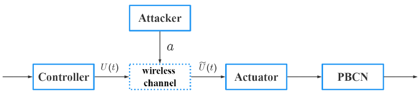
Assume that the PBCN is initially in the state at time , denoted as and it reaches the state at time under a sequence of controls with probability 1. Considering that the attacker can attack any control node and invert the value of the control node, the attack framework is shown in Figure 1. We define the possible actions at each time step as , where and for no attack, for attack on the th control node. Then, the number of actions at each state is , and the control is changed to , where is defined as follows:
Furthermore, we denote the action with no attack on any control node as . The goal of the attacker is to select the attack time point and the control node to be attacked so that the state of the PBCN reaches the target state after time , where can be chosen arbitrarily, as long as there is a sequence of controls such that . The main problems we are interested in consist of the following:
-
1.
How to choose the attack time points and the control nodes so that the state of the PBCN reach the target state after time with probability 1?
-
2.
On the basis of the previous problem, how to minimize the expectation of time points that need to be attacked?
-
3.
On the basis of the first problem, how to minimize the expectation of the number of attacks on the control node?
In some literature that use RL methods to solve the control problems on the PBCN, the state of the PBCN can be naturally set to be the state of the MDP. However, the objectives of these three problems are related to the time , so we need the states of the PBCN along with the time to be the states of MDP. Under this setting, the state set of the MDP is , and the terminal states are . The reward function of the MDP for each of the three problems are defined as follows. for problem 1),
| (10) |
for all , , and:
| (11) |
For problem 2),
| (12) |
for all , , and:
| (13) |
For problem 3),
| (14) |
for all , , and:
| (15) |
where is the Hamming weight of the action . In addition, choosing an appropriate value of in equations (12)-(15) ensures if and , then , where is the attack policy, is the expectaction of the total reward under , and is the state of PBCN at time under . Next, we analyze the value range for as follows. Since is a fixed value and the primary objective for all three problems is to guide the PBCN to the taget state, it is reasonable to choose . Then for problem 2), we have:
| (16) |
and for problem 3):
| (17) |
So, for problem 2) and for problem 3). By representing the attacked PBCN model in the MDP framework described as above, the optimal false data injection attack problems 1), 2) and 3) can be formulated as finding the strategy such that:
| (18) |
IV Algorithms for Optimal Attack Strategies of a PBCN
In this section, we introduce the QL algorithm, and give an improved QL algorithm and a modified QL algorithm to solve the optimal false data injection attack problem for the PBCN (9).
IV-A QL Algorithm for Optimal Attack on PBCN
In order to provide the attacker’s attack strategy in a model-free framework, we can use the QL algorithm. QL is a model-free, off-policy temporal difference control algorithm. The goal of the QL is to find the optimal action-value function and the action-value function is updated by the following formula:
| (19) |
Under the assumption that all the state-action pairs be visited infinitely often and a variant of the usual stochastic approximation conditions on the sequence of step-size parameters , QL has been shown to converge to the optimal action-value function with probability one [32]. The QL algorithm is shown in Algorithm 1.
Remark 1.
Algorithm 1 can solve the three interested problems. The only difference is that the reward is set in different ways. Similarly, Algorithms 2 and 3 in the sequel also can solve the three interested problems of different reward settings.
IV-B Improved QL Algorithm for Optimal Attack on PBCN
Note that the QL algorithm creates a look-up table for all state-action pairs, thus requiring a large amount of memory when the state-action space is very large, as the state-action space grows exponentially with the number of nodes and inputs. When the state-action space becomes very large, the basic QL algorithm is often unable to handle this situation due to the dramatic increase in required memory. In attack problems for a PBCN, when the state- action space becomes large, there may also be many state-action pairs that are not accessed. Let denote the number of state-action pairs that can be accessed. Then, in the attacked PBCN model, the space requirement for the action-value function is . We propose a small modification to Algorithm 1 by recording and updating the corresponding value function only when the state-action pair is encountered for the first time, such that it can be used for attack problems in large-scale PBCNs if . Under this setting, the space requirement for the action-value function is reduced from in Algorithm 1 to in Algorithm 2. In addition, note that a condition for the convergence of the QL algorithm is that all state-action pairs be visited infinitely often, which cannot be satisfied in actual processes. Therefore, the policy obtained by QL after a finite number of episodes may not be optimal, but the learning process may have experienced the optimal state-action sequence. One approach to address this is by recording the total rewards of policies encountered during the learning process for each initial state. After the learning process, we compare the total rewards of policies obtained by QL with the recorded optimal policies and select the policy with the higher expected total reward as our final policy. By combining these two methods, we obtain an improved QL algorithm shown in Algorithm 2.
Remark 2.
In Algorithm 2, we still use the same updated function (21) of the QL. Therefore, Algorithm 2 can still converge to the optimal policy with probability 1 when the conditions in the QL algorithm are satisfied.
Remark 3.
In Algorithm 2, is a list that used to record the best action sequences encountered during the learning process and is the corresponding return.
Remark 4.
In Algorithm 2, is a constant that serves as the initial value for . Since needs to be small enough such that the total reward of any policy is larger than it, can be any number as long as the condition is satisfied.
Remark 5.
In Algorithm 2, is a dict of action values, where the elements are key-value pairs. The key is the state, and the value is the corresponding action value in that state. represents the set of states that have been recorded in .
Remark 6.
Since Algorithm 2 is based on QL, the agent must choose the optimal action-value from the attack actions at each time step. However, if we use the DQN algorithm, the agent not only has to select the optimal action value from the attack actions but also update the network parameters, resulting in higher computational complexity compared to Algorithm 2. Moreover, Algorithm 2 provides better convergence guarantees than DQN.
IV-C Computational Complexity
We analyze the time and space complexity of our proposed algorithms as follows. In all the proposed algorithms, the agent must choose the optimal action-value from the attack actions at each time step, resulting in a time complexity of . In each episode out of episodes, this operation needs to be be performed times. Thus, the total time complexity of Algorithm 1 is , while Algorithm 2 includes an additional operation to find the maximum value, resulting in a total time complexity of . Now, we consider space complexity. Since it is necessary to store the values of state-action pairs, the space complexity involved here for Algorithm 1 is . The space complexity of Algorithm 2 for storing the values of state-action pairs is , where is the number of state-action pairs that can be accessed. In addition to storing the values of state-action pairs, it is necessary to record the expected total reward of policies for Algorithm 2, resulting in a space complexity of .
V Simulation Results
In this section, we show how to solve the three problems on attacked PBCN by the results obtained in the previous section. We consider two PBCN models, one with 10 nodes, 3 control inputs and another one with 28 nodes, 3 control inputs to prove the efficiency of the proposed algorithms. Since is not a very critical parameter in the simulation, we can actually choose as any number. However, taking the value of too large requires a lot of computation, so we choose as a small number. For the following two examples, we choose .
V-A Example 5.1
Consider the following PBCN model with 10 nodes and 3 control inputs, which is is similar to the model of the lactose operon in the Escherichia Coli derived from [33]:
| (20) |
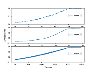
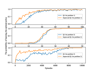
and we choose the state (0, 0, 0, 0, 1, 1, 0, 0, 0, 0) of the PBCN to be the initial state of the PBCN. The attacker aims to change the state of PBCN to the desired state (0, 0, 0, 1, 1, 1, 0, 0, 0, 0) at by tampering with the control inputs. Moreover, we choose and for problems 2), 3), respectively. As for the step size and the discount rate , we choose for all three problems, and for problem 1 and problem 2 while for problem 3. By following Algorithms 1 and 2, we obtain optimal attacks on the PBCN (20). We run 1000 independent experiments to obtain the average reward for each episode for these three problems, and the results are shown in Figure 2. As can be seen in Figure 2, the average reward increases with the number of episodes and eventually converges, implying that an optimal attack policy has been obtained. By running 100 independent experiments for different numbers of episodes, we obtain the relationship between the probability of learning the optimal attack policy and the number of episodes for both algorithms. As shown in Figure 3, the probability of learning the optimal attack policy increases with the number of episodes and eventually converges to 1 for both algorithms. However, under the same number of episodes, the probability of learning the optimal policy using Algorithm 2 is higher than that of Algorithm 1, implying that our proposed improved QL algorithm is more effective than traditional QL in solving the optimal attack problem for a PBCN.
V-B Example 5.2
Consider the following PBCN model with 28 nodes and 3 control inputs [34], which is a reduced-order model of 32-gene T-cell receptor kinetics model given in [35]:
| (21) |
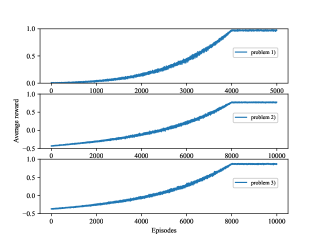
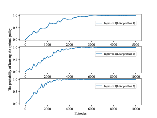
and we choose the state (0, 0, 0, 0, 1, 1, 1, 0, 0, 0, 1, 0, 0, 0, 0, 0, 0, 0, 0, 1, 1, 0, 0, 0, 0, 1, 1, 0) of the PBCN to be the initial state of the PBCN, and the desired state is (0, 0, 0, 1, 1, 1, 1, 0, 0, 0, 1, 0, 0, 1, 0, 0, 0, 0, 0, 1, 1, 0, 0, 0, 0, 1, 1, 0). Moreover, we set for all the three problems, and we choose and for problems 2) and 3), respectively. As for the step size and the discount rate , we choose and for all three problems. By following the improved QL algorithm (Algorithm 2), we can also obtain the optimal attack policy for large scale PBCN, which cannot be achieved by directly applying the traditional QL algorithm (Algorithm 1). Similar to example 5.1, the average reward on each episode for these three problems are shown in Figure 4, where one can see that the average reward increases with the number of episodes and eventually converges. Figure 5 also shows the property that the probability of learning the optimal attack policy increases with the number of episodes and eventually converges to 1.
VI Conclusion
In this paper, we have investigated optimal false data injection attack problems on PBCNs using model-free RL methods. We have proposed an improved QL algorithm to solve these problems more effectively. Additionally, our proposed algorithm can solve the optimal attack problem for some large-scale PBCNs that the standard QL algorithm cannot handle. We have provided two examples to illustrate the validity of our proposed algorithms. However, we have only discussed false data injection attack problems from the attacker’s perspective. In the future, we may study resilient control problems against the false data injection attacks proposed in this paper, such that the system can remain stable through controller design, making it more robust.
References
- [1] S. Kauffman, “Metabolic stability and epigenesis in randomly constructed genetic nets,” J. Theoret. Biol., vol. 22, no. 3, pp. 437–467, 1969.
- [2] M. Meng, J. Lam, J. Feng, and K. Cheung, “Stability and stabilization of Boolean networks with stochastic delays,” IEEE Trans. Autom. Control, vol. 64, no. 2, pp. 790–796, 2019.
- [3] H. Li, X. Yang, and S. Wang, “Robustness for stability and stabilization of Boolean networks with stochastic function perturbations,” IEEE Trans. Automat. Control, vol. 66, no. 3, pp. 1231–1237, 2021.
- [4] M. Imani, E. R. Dougherty, and U. Braga-Neto, “Boolean Kalman filter and smoother under model uncertainty,” Automatica, vol. 111, p. 108609, 2020.
- [5] J. Heidel, J. Maloney, C. Farrow, and J. Rogers, “Finding cycles in synchronous Boolean networks with applications to biochemical systems,” Internat. J. Bifur. Chaos, vol. 13, no. 3, pp. 535–552, 2003.
- [6] Y. Guo, P. Wang, W. Gui, and C. Yang, “Set stability and set stabilization of boolean control networks based on invariant subsets,” Automatica, vol. 61, pp. 106–112, 2015.
- [7] I. Shmulevich, E. Dougherty, S. Kim, and W. Zhang, “Probabilistic Boolean networks: a rule-based uncertainty model for gene regulatory networks,” Bioinformatics, vol. 18, no. 2, pp. 261–274, 2002.
- [8] Z. Ma, Z. J. Wang, and M. J. McKeown, “Probabilistic Boolean network analysis of brain connectivity in parkinson’s disease,” IEEE Journal of selected topics in signal processing, vol. 2, no. 6, pp. 975–985, 2008.
- [9] P. J. Rivera Torres, E. I. Serrano Mercado, and L. Anido Rifón, “Probabilistic Boolean network modeling and model checking as an approach for DFMEA for manufacturing systems,” Journal of Intelligent Manufacturing, vol. 29, no. 6, pp. 1393–1413, 2018.
- [10] P. Trairatphisan, A. Mizera, J. Pang, A. A. Tantar, J. Schneider, and T. Sauter, “Recent development and biomedical applications of probabilistic Boolean networks,” Cell communication and signaling, vol. 11, no. 1, pp. 1–25, 2013.
- [11] J.-W. Gu, W.-K. Ching, T.-K. Siu, and H. Zheng, “On modeling credit defaults: A probabilistic Boolean network approach,” Risk and Decision Analysis, vol. 4, no. 2, pp. 119–129, 2013.
- [12] P. J. Rivera Torres, E. I. Serrano Mercado, and L. Anido Rifón, “Probabilistic Boolean network modeling of an industrial machine,” Journal of Intelligent Manufacturing, vol. 29, no. 4, pp. 875–890, 2018.
- [13] C. Yang, J. Wu, X. Ren, W. Yang, H. Shi, and L. Shi, “Deterministic sensor selection for centralized state estimation under limited communication resource,” IEEE Trans. Signal Process., vol. 63, no. 9, pp. 2336–2348, 2015.
- [14] S. H. Ahmed, G. Kim, and D. Kim, “Cyber physical system: Architecture, applications and research challenges,” in 2013 IFIP Wireless Days (WD), pp. 1–5, 2013.
- [15] Y. Tang, D. Zhang, D. W. C. Ho, and F. Qian, “Tracking control of a class of cyber-physical systems via a flexray communication network,” IEEE Trans. Cybernetics, vol. 49, no. 4, pp. 1186–1199, 2019.
- [16] A. Roli, M. Manfroni, C. Pinciroli, and M. Birattari, “On the design of Boolean network robots,” in European Conference on the Applications of Evolutionary Computation, pp. 43–52, 2011.
- [17] J. Zhang, J. Sun, and H. Lin, “Optimal DoS attack schedules on remote state estimation under multi-sensor round-robin protocol,” Automatica, vol. 127, p. 109517, 2021.
- [18] J. Markoff, “A silent attack, but not a subtle one,” The New York Times, Sept. 26, 2010.
- [19] T. Sui and X. Sun, “The vulnerability of distributed state estimator under stealthy attacks,” Automatica, vol. 133, p. 109869, 2021.
- [20] H. Zhang, P. Cheng, L. Shi, and J. Chen, “Optimal Denial-of-Service attack scheduling with energy constraint,” IEEE Trans. Autom. Control, vol. 60, no. 11, pp. 3023–3028, 2015.
- [21] B. Chen, D. W. C. Ho, G. Hu, and L. Yu, “Secure fusion estimation for bandwidth constrained cyber-physical systems under replay attacks,” IEEE Trans. Cybernetics, vol. 48, no. 6, pp. 1862–1876, 2018.
- [22] Y. Liu, P. Ning, and M. K. Reiter, “False data injection attacks against state estimation in electric power grids,” in 16th ACM Conference on Computer and Communications Security, pp. 21–32, 2009.
- [23] Y. Mo, R. Chabukswar, and B. Sinopoli, “Detecting integrity attacks on SCADA systems,” IEEE Transactions on Control Systems Technology, vol. 22, no. 4, pp. 1396–1407, 2013.
- [24] W. Yang, Y. Zhang, G. Chen, C. Yang, and L. Shi, “Distributed filtering under false data injection attacks,” Automatica, vol. 102, pp. 34–44, 2019.
- [25] R. S. Sutton and A. G. Barto, Reinforcement learning: An introduction. MIT press, 2018.
- [26] L. Buşoniu, T. de Bruin, D. Tolić, J. Kober, and I. Palunko, “Reinforcement learning for control: Performance, stability, and deep approximators,” Annual Reviews in Control, vol. 46, pp. 8–28, 2018.
- [27] S. Preitl, R.-E. Precup, Z. Preitl, S. Vaivoda, S. Kilyeni, and J. K. Tar, “Iterative feedback and learning control. servo systems applications,” IFAC Proceedings Volumes, vol. 40, no. 8, pp. 16–27, 2007.
- [28] R.-C. Roman, R.-E. Precup, and E. M. Petriu, “Hybrid data-driven fuzzy active disturbance rejection control for tower crane systems,” European Journal of Control, vol. 58, pp. 373–387, 2021.
- [29] C. J. C. H. Watkins, Learning from delayed rewards. Ph.d. thesis, King’s College, Cambridge United Kingdom, 1989.
- [30] Z. Liu, J. Zhong, Y. Liu, and W. Gui, “Weak stabilization of Boolean networks under state-flipped control,” IEEE Transactions on Neural Networks and Learning Systems, vol. published online, 2021.
- [31] P. B. Dimitri et al., “Dynamic programming and optimal control,” Athena Scientific, vol. 1-2, 1995.
- [32] C. J. Watkins and P. Dayan, “Q-learning,” Machine learning, vol. 8, no. 3, pp. 279–292, 1992.
- [33] A. Veliz-Cuba and B. Stigler, “Boolean models can explain bistability in the lac operon,” Journal of computational biology, vol. 18, no. 6, pp. 783–794, 2011.
- [34] A. Acernese, A. Yerudkar, L. Glielmo, and C. Del Vecchio, “Double deep-q learning-based output tracking of probabilistic boolean control networks,” IEEE Access, vol. 8, pp. 199254–199265, 2020.
- [35] K. Zhang and K. H. Johansson, “Efficient verification of observability and reconstructibility for large Boolean control networks with special structures,” IEEE Transactions on Automatic Control, vol. 65, no. 12, pp. 5144–5158, 2020.