Magneto-interferometry of multiterminal Josephson junctions

Abstract

We report a theoretical study of multiterminal Josephson junctions under the influence of a magnetic field $B$. We consider a ballistic rectangular two-dimensional metal $N_{0}$ connected by the edges to the left, right, top and bottom superconductors $S_{L}$, $S_{R}$, $S_{T}$ and $S_{B}$, respectively. We numerically calculate in the long-junction limit the critical current $I_{c}$ versus $B$ between $S_{L}$ and $S_{R}$ for various aspect ratios, with $S_{T}$ and $S_{B}$ playing the role of superconducting mirrors. We find $I_{c}$ to be enhanced by orders of magnitude, especially at long distance, due to the phase rigidity provided by the mirrors. We obtain superconducting quantum interference device-like magnetic oscillations. With symmetric couplings, the self-consistent superconducting phase variables of the top and bottom mirrors take the values $0$ or $\pi$, as for emerging Ising degrees of freedom. We propose a simple effective Josephson junction circuit model that is compatible with these microscopic numerical calculations. From the $I_{c}(B)$ patterns we infer where the supercurrent flows in various device geometries. In particular in the elongated geometry, we show that the supercurrent flows between all pairs of contacts, which allows exploring the full phase space of the relevant phase differences.

I Introduction

Superconducting multiterminal systems have recently attracted considerable attention. While early theoretical works already predicted unusual behaviour of these more complex Josephson junctions Ouboter1995 ; Amin2001 ; Amin2002 ; Amin2002a , the later ones demonstrated that these systems may host several exotic phenomena such as correlations among Cooper pairs known as the quartets Freyn2011 ; Melin2016 ; Jonckheere2013 ; Melin2017 ; Melin2019 ; Doucot2020 ; Melin2020 ; Melin2020a ; Melin2021 ; Melin2022 ; Melin2023 ; Melin2023a ; Keleri2023 as well as Weyl points singularities and nontrivial topology in the Andreev bound state spectrum Riwar2016 ; Eriksson2017 ; Xie2017 ; Xie2018 ; Deb2018 ; Venitucci2018 ; Gavensky2018 ; Klees2020 ; Fatemi2021 ; Peyruchat2021 ; Weisbrich2021 ; Chen2021 ; Chen2021a ; Repin2022 ; Gavensky2023 , and the energy level repulsion in Andreev molecules Pillet2019 ; Pillet2020 ; Kornich2019 ; Pillet2023 . Following these theoretical efforts, recent experiments have reported the detection of Cooper quartets Pfeffer2014 ; Cohen2018 ; Huang2022 ; Graziano2022 , the observation of Floquet-Andreev states Park2022 , the studies of Andreev molecules Kurtossy2021 ; Coraiola2023 ; Matsuo2023 ; Matsuo2023a , the multiterminal superconducting diode effect Gupta2023 ; Zhang2023 , in addition to other results using numerous different types of superconducting weak links  Matsuo2022 ; Draelos2019 ; Pankratova2020 ; Graziano2020 ; Arnault2021 ; Arnault2021 ; Khan2021 ; Arnault2022 ; Zhang2022 .

The common ground to these models and experiments is related to the fact that the weak links are connected by, at least, three superconducting contacts. Indeed, in comparison to its two leads counterparts, the supercurrent flow in multiterminal Josephson junctions may appear non-trivial. Seminal works showed that the supercurrent distribution could be probed by analyzing the interference pattern induced by the application of a magnetic flux across two-terminal Josephson junctions Rowell1963 ; Dynes1971 ; Zappe1975 ; BaronePaternoBook ; Tinkham . Therefore, this interferometric pattern strongly depends on the device geometry and where the supercurrent flows Barzykin1999 ; Kikuchi2000 ; Angers2008 ; Chiodi2012 ; Amado2013 ; Hart2014 ; Allen2016 ; Meier2016 ; Amet2016 ; Kraft2018 ; Irfan2018 ; Pandey2022 ; Chu2023 . As shown by Dynes and Fulton Dynes1971 , in two-terminal Josephson junctions, the magnetic field dependence of the critical current is related to the supercurrent density distribution across the device by an inverse Fourier transform as long as the supercurrent density is constant along the current flow. However, alternative models are needed in the case of non-homogeneous supercurrent density Kraft2018 or non-regular shapes Irfan2018 ; Chu2023 .

To our knowledge, no theories exploring the current flow and the corresponding magneto-interferometric pattern in multi-terminal Josephson junctions are available so far. Here, we present a microscopic model allowing us to calculate the magnetic field dependence of the critical current in various configurations (see Fig. 1). Our calculations are based on a large-gap Hamiltonian in which the supercurrent is triggered by the tracer of the phase of the vector potential, i.e. we calculate the critical current pattern as a function of the magnetic field. While we recover the standard two-terminal interferometric patterns, we show that the additional lead drastically modifies the magnetic field dependence of the critical current. With four terminals, our calculations reveal that the supercurrent visits all of the superconducting leads, which could result from a kind of ergodicity. This notion of ergodicity was lately pointed out via the studies of the critical current contours (CCCs) in four-terminal Josephson junctions, as a function of two different biasing currents Pankratova2020 ; Melin2023a . Consistency was demonstrated Pankratova2020 between the experiments on the CCCs and Random Matrix Theory, where the scattering matrix bridges all of the superconducting leads. Considering disorder in the short-junction limit, quantum chaos leads to ergodicity in the sense of Andreev bound states (ABS) coupling all of the superconducting leads. The supercurrent significantly visits all of those, thus being sensitive to $n-1$ independent phase differences, a number that is however reduced by the additional constraints of current conservation imposed by the external sources. In the other limit of large-scale devices, another recent work Melo2022 pointed out the relevance of long-range effects in multiterminal configurations, as the result of the phase rigidity.

Here, we also find long-range propagation of the supercurrent in three- or four-terminal geometry having one or two superconducting mirrors respectively, due to the phase rigidity in the leads under zero-current bias condition. In the four-terminal geometries, the leads $S_{L}$, $S_{R}$, $S_{T}$ and $S_{B}$ are connected to the left, right, top and bottom sides of the rectangular normal-metallic conductor $N_{0}$ and $S_{T},\,S_{B}$ are laterally connected on top and bottom, being superconducting mirrors in open circuit, as shown Fig. 1c and Fig. 1d. For the elongated geometry along the horizontal $x$-axis direction (see Fig. 1c), the four-terminal magnetic oscillations of the critical current resemble the pattern of a superconducting quantum interference device (SQUID) because of the interfering supercurrent paths propagating in $S_{T}$ and $S_{B}$ over long distance. The critical current in the horizontal direction is controlled by the phases $\varphi_{T}$ and $\varphi_{B}$ of the top and bottom superconductors $S_{T}$ and $S_{B}$. Symmetry in the hopping amplitudes connecting $N_{0}$ to the four superconductors leads to the discrete values $\varphi_{T},\,\varphi_{B}=0$ or $\pi$, as for emerging Ising degrees of freedom.

Finally, a simple phenomenological Josephson junction circuit model is proposed for devices elongated in the horizontal direction. In this model, both of the superconducting phase variables $\varphi_{T}$ and $\varphi_{B}$ enter the critical current via their difference $\varphi_{T}-\varphi_{B}$, which originates from the large Josephson energy coming from the extended interfaces parallel to the horizontal direction.

The paper is organized as follows. The model and Hamiltonians are presented in Sec. II. The numerical results are presented and discussed in Sec. III. Sec. IV presents a phenomenological Josephson junction circuit model. Concluding remarks are provided in Sec. V.

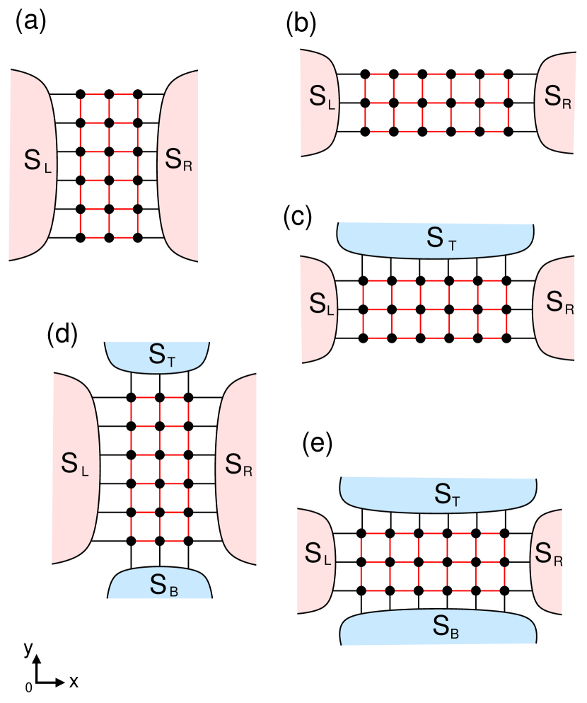
Figure 1: Schematics of the considered two- and multiterminal Josephson geometries. The superconductors $S_{T}$ and $S_{B}$ on top and bottom are in open circuit, that is, they are superconducting mirrors, and we calculate the current flowing horizontally from $S_{L}$ to $S_{R}$. A four-terminal device with $N=3$ and $M=6$ is shown on panel a, i.e. a device with $M/N\gtrsim 1$ elongated in the vertical $y$-axis direction. A two-terminal device elongated in the horizontal $x$-axis direction is shown on panel b with $N=6$ and $M=3$, i.e. with $M/N\lesssim 1$. Panels c, d and e feature three- or four-terminal devices containing a single or two superconducting mirrors, and elongated along the $x$- or $y$-axis directions.

II Model and Hamiltonians

In this section, we define the Hamiltonian of the devices shown in Fig. 1. The Hamiltonians of each part of the circuit are provided in subsection II.1. The large-gap Hamiltonian of the entire structure is presented in subsection II.2, and the boundary conditions in the presence of a magnetic field are next discussed in subsection II.3. The algorithm is presented in Sec. II.4.

II.1 General Hamiltonians

In this subsection, we introduce the Hamiltonians of the superconductor, the central normal-metal conductor and the coupling between them.

The superconductors are described by the BCS Hamiltonian

$$\hat{\cal H}_{BCS} = -W\sum_{\langle i,j\rangle}\sum_{\sigma_{z}=\uparrow,\downarrow}\left(c_{i,\sigma_{z}}^{+}c_{j,\sigma_{z}}+c_{j,\sigma_{z}}^{+}c_{i,\sigma_{z}}\right)$$ (1)

$$- \Delta\sum_{k}\left(\exp\left(i\varphi_{k}\right)c_{k,\uparrow}^{+}c_{k,\downarrow}^{+}+\exp\left(-i\varphi_{k}\right)c_{k,\downarrow}c_{k,\uparrow}\right),$$ (2)

where the summation in the first term is over all pairs of neighboring tight-binding sites $\langle i,j\rangle$ and over the projection $\sigma_{z}$ on the spin quantization axis, that is the $z$-axis. The first term given by Eq. (1) corresponds to the kinetic energy, i.e. to spin-$\sigma_{z}$ electrons hopping between neighboring tight-binding sites on a square-lattice. The second term given by Eq. (2) is the mean field BCS pairing term, with superconducting phase variable $\varphi_{k}$ at the tight-binding site $k$. The superconducting phase variables $\varphi_{k}$ take different values between different superconducting leads and the $\varphi_{k}$s are assumed to be uniform within each of those since we handle weak currents throughout the paper. In order to reduce the computational expanses, we carry out the calculations in a regime where the superconducting gap is the largest energy scale, leading to a large-gap Hamiltonian for the entire device connected to the superconducting leads. This approach will be justified from qualitative agreement with the known Fraunhofer pattern like in a two-terminal configuration (i.e. with vanishingly small coupling to the top and bottom $S_{T}$ and $S_{B}$ respectively, see Figs. 1a and 1b).

The central ballistic normal-metallic conductor $N_{0}$ is described by the square-lattice tight-binding Hamiltonian on a rectangle of dimensions $Na_{0}\times Ma_{0}$ in the horizontal $x$- and vertical $y$-axis directions respectively, where $a_{0}$ is the lattice spacing:

$$\hat{\cal H}_{\Sigma^{(0)}}=-\Sigma^{(0)}\sum_{\langle i,j\rangle}\sum_{\sigma_{z}=\uparrow,\downarrow}\left(c_{i,\sigma_{z}}^{+}c_{j,\sigma_{z}}+c_{j,\sigma_{z}}^{+}c_{i,\sigma_{z}}\right),$$ (3)

with hopping amplitude $\Sigma^{(0)}$. Eq. (3) is intended to qualitatively capture a two-dimensional conductor at high charge carrier density, and thus presenting a well-defined extended Fermi surface. We assume that a finite gate voltage is applied to the square-lattice tight-binding Hamiltonian of Eq. (3) in such a way as to avoid the square-lattice midband singularities:

$$\hat{\cal H}_{g}=-W_{g}\sum_{k,\sigma_{z}}c_{k,\sigma_{z}}^{+}c_{k,\sigma_{z}}.$$ (4)

The contacts between the normal and superconducting leads are captured by the following tight-binding Hamiltonian with hopping amplitude $\Sigma^{(1)}$:

$$\hat{\cal H}_{\Sigma^{(1)}}=-\Sigma^{(1)}\sum_{\langle i^{\prime},j^{\prime}\rangle}\sum_{\sigma_{z}=\uparrow,\downarrow}\left(c_{i^{\prime},\sigma_{z}}^{+}c_{j^{\prime},\sigma_{z}}+c_{j^{\prime},\sigma_{z}}^{+}c_{i^{\prime},\sigma_{z}}\right),$$ (5)

where $\sum_{\langle i^{\prime},j^{\prime}\rangle}$ runs over all tight-binding sites on both sides of the contact.

The magnetic field is included by adding a phase to the hopping amplitudes between the tight-binding sites $a$ and $b$:

$$\Sigma_{a\rightarrow b}\rightarrow\Sigma_{a\rightarrow b}\exp\left(\frac{ie}{\hbar}\int_{a}^{b}{\bf A}\,.\,d{\bf s}\right),$$ (6)

where ${\bf A}$ is the vector potential. In addition, the absence of screening currents on the superconducting sides of the normal metal-superconductor boundaries will be taken into account according to the forthcoming subsection II.3.

II.2 Large-gap Hamiltonian at zero magnetic field

In this subsection, we consider that the superconducting gaps are the largest energy scales. This yields a large-gap Hamiltonian for the entire device, which will afterwards be treated via exact diagonalizations. The DC-Josephson currents are obtained from numerically differentiating the ground state energy with respect to the superconducting phase variable of the corresponding terminal. Making the approximation of a large superconducting gap was developed over the recent years, see for instance Refs. Zazunov2003, ; Meng2009, ; Melin2021, ; Klees2020, . Reaching numerical efficiency for large-scale devices is the main motivation for this large-gap limit.

Large-gap Hamiltonian from wave-functions: Now, we present a wave-function calculation which yields the large-gap Hamiltonian. Using generic compact matrix notations, the starting-point Nambu Hamiltonian is expressed as the sum of three terms:

(i) The infinite Nambu matrix of the superconducting tight-binding Hamiltonian $\hat{\cal H}_{S,S}$ is deduced from the BCS Hamiltonian $\hat{\cal H}_{BCS}$ in Eqs. (1)-(2). Those superconducting leads are generically denoted as $S_{1},\,...\,,S_{n}$ and $\hat{\cal H}_{S,S}$ is a matrix gathering all of the $\hat{\cal H}_{S_{p},S_{p}}$, with $p=1,\,...,\,n$.

In order to illustrate the discussion, we consider for simplicity that the lead $S_{p}$ contains two tight-binding sites labeled by “1” and “2”, which yields the following $4\times 4$ Nambu Hamiltonian $\hat{\cal H}_{S_{p},S_{p}}$:

$$\hat{\cal H}_{S_{p},S_{p}}=\left(\begin{array}[]{cccc}0&\Delta_{p}e^{i\varphi_{p}}&-W_{1,2}&0\\ \Delta_{p}e^{-i\varphi_{p}}&0&0&W_{1,2}\\ -W_{2,1}&0&0&\Delta_{p}e^{i\varphi_{p}}\\ 0&W_{2,1}&\Delta_{p}e^{-i\varphi_{p}}&0\end{array}\right).$$ (7)

With a three-site tight-binding cluster, we obtain the following $6\times 6$ Nambu Hamiltonian:

$$\hat{\cal H}_{S_{p},S_{p}}=$$ (8)

$$\left(\begin{array}[]{cccccc}0&\Delta_{p}e^{i\varphi_{p}}&-W_{1,2}&0&-W_{1,3}&0\\ \Delta_{p}e^{-i\varphi_{p}}&0&0&W_{1,2}&0&W_{1,3}\\ -W_{2,1}&0&0&\Delta_{p}e^{i\varphi_{p}}&-W_{2,3}&0\\ 0&W_{2,1}&\Delta_{p}e^{-i\varphi_{p}}&0&0&W_{2,3}\\ -W_{3,1}&0&-W_{3,2}&0&0&\Delta_{p}e^{i\varphi_{p}}\\ 0&W_{3,1}&0&W_{3,2}&\Delta_{p}e^{-i\varphi_{p}}&0\end{array}\right),$$ (15)

where the three tight-binding sites are labeled by $1,\,2$ and $3$. The matrices in Eqs. (7) and (8) can be extrapolated to an infinite number of tight-binding sites, also taking the connectivity of the underlying lattice into account. Finally, all of the $\hat{\cal H}_{S_{p},S_{p}}$ are concatenated into the global $\hat{\cal H}_{S,S}$ matrix.

(ii) The finite Nambu matrix rectangular normal-metal tight-binding lattice Hamiltonian $\hat{\cal H}_{N_{0},N_{0}}$ is deduced from $\hat{\cal H}_{\Sigma^{(0)}}$ in Eq. (3) and $\hat{\cal H}_{g}$ in Eq. (4). The Nambu Hamiltonian $\hat{\cal H}_{N_{0},N_{0}}$ takes the following form for the two tight-binding sites labeled by $1$ and $2$:

$$\hat{\cal H}_{N_{0},N_{0}}^{2\times 2}=\left(\begin{array}[]{cccc}W_{g}&0&-\Sigma^{(0)}_{1,2}&0\\ 0&-W_{g}&0&\Sigma^{(0)}_{1,2}\\ -\Sigma^{(0)}_{2,1}&0&W_{g}&0\\ 0&\Sigma^{(0)}_{2,1}&0&-W_{g}\end{array}\right).$$ (16)

We obtain the following with the three tight-binding sites labeled by $1$, $2$ and $3$:

$$\hat{\cal H}_{N_{0},N_{0}}^{3\times 3}=$$ (17)

$$\left(\begin{array}[]{cccccc}W_{g}&0&-\Sigma^{(0)}_{1,2}&0&-\Sigma^{(0)}_{1,3}&0\\ 0&-W_{g}&0&\Sigma^{(0)}_{1,2}&0&\Sigma^{(0)}_{1,3}\\ -\Sigma^{(0)}_{2,1}&0&W_{g}&0&-\Sigma^{(0)}_{2,3}&0\\ 0&\Sigma^{(0)}_{2,1}&0&-W_{g}&0&\Sigma^{(0)}_{2,3}\\ -\Sigma^{(0)}_{3,1}&0&-\Sigma^{(0)}_{3,2}&0&W_{g}&0\\ 0&\Sigma^{(0)}_{3,1}&0&\Sigma^{(0)}_{3,2}&0&-W_{g}\end{array}\right),$$ (24)

and Eqs. (16)-(17) are easily generalized to an arbitrary number of entries.

(iii) The finite Nambu matrix of the couplings $\hat{\cal H}_{N_{0},S}$ and $\hat{\cal H}_{S,N_{0}}$ between the superconductors $S_{p}$ and the normal region $N_{0}$ is deduced from $\hat{\cal H}_{\Sigma^{(1)}}$ in Eq. (5). The Nambu Hamiltonian $\hat{\cal H}_{N_{0},S_{p}}$ takes the following form with interfaces made with the two tight-binding sites labeled by $1$ and $2$:

$$\hat{\cal H}_{N_{0},S_{p}}^{2\times 2}=\left(\begin{array}[]{cccc}0&0&-\Sigma^{(1)}_{1,2}&0\\ 0&0&0&\Sigma^{(1)}_{1,2}\\ -\Sigma^{(1)}_{2,1}&0&0&0\\ 0&\Sigma^{(1)}_{2,1}&0&0\end{array}\right),$$ (25)

and we obtain the following for interfaces made with the three tight-binding sites labeled by $1$, $2$ and $3$:

$$\hat{\cal H}_{N_{0},S_{p}}^{3\times 3}=$$ (26)

$$\left(\begin{array}[]{cccccc}0&0&-\Sigma^{(1)}_{1,2}&0&-\Sigma^{(1)}_{1,3}&0\\ 0&0&0&\Sigma^{(1)}_{1,2}&0&\Sigma^{(1)}_{1,3}\\ -\Sigma^{(1)}_{2,1}&0&0&0&-\Sigma^{(1)}_{2,3}&0\\ 0&\Sigma^{(1)}_{2,1}&0&0&0&\Sigma^{(1)}_{2,3}\\ -\Sigma^{(1)}_{3,1}&0&-\Sigma^{(1)}_{3,2}&0&0&0\\ 0&\Sigma^{(1)}_{3,1}&0&\Sigma^{(1)}_{3,2}&0&0\end{array}\right),$$ (33)

and the matrices appearing in Eqs. (25)-(26) can be extended to an arbitrary number of entries.

The components of the Bogoliubov-de Gennes wave-functions are denoted as $\psi_{N_{0}}$ and $\psi_{S}$ for the normal conductor $N_{0}$ and the $n$ superconducting leads $S_{p}$ respectively, with $p=1,\,...,\,n$. Each of the $\psi_{N_{0}}$ and $\psi_{S}$ is defined on the normal-metallic tight-binding graph $N_{0}$ and in all tight-binding sites of each superconductor $S_{p}$.

The overall infinite Nambu Hamiltonian $\hat{\cal H}$ takes the following matrix form:

$$\hat{\cal H}=\left(\begin{array}[]{cc}\hat{\cal H}_{N_{0},N_{0}}&\hat{\cal H}_{N_{0},S}\\ \hat{\cal H}_{S,N_{0}}&\hat{\cal H}_{S,S}\end{array}\right).$$ (34)

The Bogoliubov-de Gennes eigenvalue equation is defined as

$$\hat{\cal H}\left(\begin{array}[]{c}\psi_{N_{0}}\\ \psi_{S}\end{array}\right)=\omega\left(\begin{array}[]{c}\psi_{N_{0}}\\ \psi_{S}\end{array}\right),$$ (35)

where $\omega$ is the energy, and Eq. (35) leads to the following set of equations:

$$\hat{\cal H}_{{N_{0}},{N_{0}}}\psi_{N_{0}}+\hat{\cal H}_{{N_{0}},S}\psi_{S} = \omega\psi_{N_{0}}$$ (36)

$$\hat{\cal H}_{S,{N_{0}}}\psi_{N_{0}}+\hat{\cal H}_{S,S}\psi_{S} = \omega\psi_{S},$$ (37)

where Eq. (36) and Eq. (37) contain a finite and an infinite number of equations respectively. Eq. (37) is written as follows:

$$\psi_{S}=\left(\omega-\hat{\cal H}_{S,S}\right)^{-1}\hat{\cal H}_{S,{N_{0}}}\psi_{N_{0}}.$$ (38)

Eq. (38) is now specialized to the Nambu components of the superconducting Green’s functions defined on the superconducting side of the coupling Nambu Hamiltonians $\hat{\cal H}_{{N_{0}},S}$ and $\hat{\cal H}_{S,{N_{0}}}$. Then, inserting Eq. (38) into Eq. (36) leads to an eigenvalue problem for a finite number of linear equations:

$$\hat{\cal H}_{{N_{0}},{N_{0}}}\psi_{N_{0}}+\hat{\cal H}_{{N_{0}},S}\left(\omega-\hat{\cal H}_{S,S}\right)^{-1}\hat{\cal H}_{S,{N_{0}}}\psi_{N_{0}}=\omega\psi_{N_{0}}.$$ (39)

This defines the effective self-energy $\hat{\Sigma}_{eff}(\omega)$ as

$$\hat{\Sigma}_{eff}(\omega)\psi_{N_{0}}=\omega\psi_{N_{0}},$$ (40)

with

$$\hat{\Sigma}_{eff}(\omega) = \hat{\cal H}_{{N_{0}},{N_{0}}}+\hat{\cal H}_{{N_{0}},S}\left(\omega-\hat{\cal H}_{S,S}\right)^{-1}\hat{\cal H}_{S,{N_{0}}}$$ (41)

$$= \hat{\cal H}_{{N_{0}},{N_{0}}}+\hat{\Sigma}_{{N_{0}},S}^{(1)}\hat{g}_{S,S}(\omega)\hat{\Sigma}_{S,{N_{0}}}^{(1)},$$ (42)

where

$$\hat{g}_{S,S}(\omega)=\left(\omega-\hat{\cal H}_{S,S}\right)^{-1}$$ (43)

is the resolvent (i.e. the Green’s function) of the infinite superconducting leads and $\hat{\Sigma}_{{N_{0}},S}^{(1)}$ and $\hat{\Sigma}_{S,{N_{0}}}^{(1)}$ are the Nambu hopping amplitudes in $\hat{\cal H}_{{N_{0}},S}$ and $\hat{\cal H}_{S,{N_{0}}}$ respectively, see also Eq. (5).

Up to this point, the superconducting gap was finite but now, we take the limit of a large gap where $\hat{g}_{S,S}(\omega)$ becomes independent on the energy $\omega$, i.e. $\hat{g}_{S,S}(\omega)\equiv\hat{g}_{S,S}$ [see the forthcoming Eqs. (48)-(54) for the expression of the superconducting Green’s functions.] The effective self-energy $\hat{\Sigma}_{eff}(\omega)$ in Eqs. (41)-(42) takes the form of the following energy-independent effective Hamiltonian:

$$\hat{\Sigma}_{eff}(\omega)\equiv\hat{\cal H}_{eff}=\hat{\cal H}_{{N_{0}},{N_{0}}}+\hat{\Sigma}_{{N_{0}},S}^{(1)}\hat{g}_{S,S}\hat{\Sigma}_{S,{N_{0}}}^{(1)}.$$ (44)

Large-gap Hamiltonian from Green’s functions: The large-gap Hamiltonian given by Eq. (44) can also be obtained from the Dyson equations, see Ref. Melin2021, . Namely, the fully dressed Green’s function $\hat{G}_{{N_{0}},{N_{0}}}(\omega)$ at the energy $\omega$ is calculated as follows:

$$\hat{G}_{{N_{0}},{N_{0}}}(\omega) = \hat{g}_{{N_{0}},{N_{0}}}(\omega)$$

$$+\hat{g}_{{N_{0}},{N_{0}}}(\omega)\hat{\Sigma}_{{N_{0}},S}^{(1)}\hat{G}_{S,{N_{0}}}(\omega)$$

$$= \hat{g}_{{N_{0}},{N_{0}}}(\omega)$$

$$+\hat{g}_{{N_{0}},{N_{0}}}(\omega)\hat{\Sigma}_{{N_{0}},S}^{(1)}\hat{g}_{S,S}(\omega)\hat{\Sigma}_{S,{N_{0}}}^{(1)}\hat{G}_{{N_{0}},{N_{0}}}(\omega).$$

Eq. (II.2) is written as

$$\hat{G}_{{N_{0}},{N_{0}}}(\omega)=\left[\omega-\hat{\Sigma}_{eff}(\omega)\right]^{-1},$$ (47)

where, in the large-gap approximation, the effective self-energy $\hat{\Sigma}_{eff}(\omega)$ given by Eqs. (41)-(42) takes the form of the energy-$\omega$ independent Hamiltonian $\hat{\cal H}_{eff}$ given by Eq. (44), as it was obtained from this compact Green’s function calculation.

Superconducting Green’s functions: Now, we provide the expression of the superconducting Green’s function $\hat{g}_{S_{p},S_{p}}$ appearing in Eq. (44), and we specifically demonstrate that $\hat{g}_{S_{p},S_{p}}(\omega)\equiv\hat{g}_{S_{p},S_{p}}$ is independent on the energy $\omega$. The advanced local superconducting Green’s function of lead $S_{p}$ takes the following form in the presence of a finite gap:

$$\hat{g}_{S_{p},S_{p}}(\omega)=$$ (48)

$$\frac{1}{W\sqrt{|\Delta|^{2}-(\omega-i\eta)^{2}}}\left(\begin{array}[]{cc}-\omega&|\Delta|e^{i\varphi_{p}}\\ |\Delta|e^{-i\varphi_{p}}&-\omega\end{array}\right),$$ (51)

where $\eta$ is a small line-width broadening, i.e. the so-called Dynes parameter Kaplan1976 ; Dynes1978 ; Pekola2010 ; Saira2012 . Eq. (48) can be found in many papers. For instance, this Eq. (48) is the starting point of the current-voltage characteristics calculations in voltage-biased superconducting weak links Cuevas1996 .

The following is obtained in the large-gap approximation:

$$\hat{g}_{S_{p},S_{p}} = \frac{1}{W}\left(\begin{array}[]{cc}0&e^{i\varphi_{p}}\\ e^{-i\varphi_{p}}&0\end{array}\right),$$ (54)

where Eq. (54) is energy-independent, as it was anticipated in the above discussion. This Eq. (54) is next inserted into the expression Eq. (44) of the large-gap Hamiltonian, which is next numerically treated with exact diagonalizations.

II.3 Boundary conditions

In this subsection, we discuss how the large-gap Hamiltonian given by Eq. (44) is modified in the presence of a finite value for the magnetic field applied perpendicularly to the two-dimensional structure. In the presence of a vector potential ${\bf A}$, we make the substitution ${\bf p}\rightarrow{\bf p}+e{\bf A}$ for the momentum, and ${\bf j}\rightarrow(e\hbar/m)\left[{\bf\nabla}\varphi+(2e/\hbar){\bf A}\right]$ for the supercurrent ${\bf j}$, where $\varphi$ denotes the superconducting phase variable. The vector potential is expressed in the gauge $A_{x}=-By/2$ and $A_{y}=Bx/2$, where $B$ is the magnetic field.

Now, we calculate how a Cooper pair crosses the left contact from the superconductor $S_{L}$ at coordinates $(x=x_{L}-a_{0},\,y)$ to the corresponding tight-binding site at $(x=x_{L},\,y)$ in the normal metal. Considering first the left superconductor, we implement $\nabla_{y}\varphi+(2e/\hbar)A_{y}=0$ along the $S_{L}$-${N_{0}}$ interface, leading to

$$\varphi_{y}=-\frac{B(x_{L}-a_{0})y}{\Phi^{\prime}_{0}}+\varphi_{L}^{(0)},$$ (55)

where $\Phi^{\prime}_{0}=\hbar/e=\Phi_{0}/2\pi$, with $\Phi_{0}=h/e$ the superconducting flux quantum. In a second step, we integrate the phase gradient ${\bf\nabla}\varphi+(2e/\hbar){\bf A}$ in the horizontal direction across the $S_{L}$-${N_{0}}$ interface:

$$\int_{x_{L}}^{x_{L}-a_{0}}\left({\bf\nabla}\varphi+\frac{2e}{\hbar}{\bf A}\right)\,.\,d{\bf s}=\frac{Bya_{0}}{\Phi^{\prime}_{0}}+\varphi_{y}.$$ (56)

Overall, we deduce the phase

$$\varphi_{L}^{(0)}-\frac{Byx_{L}}{\Phi^{\prime}_{0}}+\frac{2Bya_{0}}{\Phi^{\prime}_{0}},$$ (57)

where $\varphi_{L}^{(0)}$ is the superconducting phase variable of the left superconductor. The following self-energy is then included in the normal-metal Hamiltonian on the left-hand-side of the rectangular tight-binding lattice, i.e. at coordinate $(x=x_{L},\,y)$:

$$\Gamma_{loc}^{(Left)}(y)=-\frac{(\Sigma^{(1)})^{2}}{W}e^{i\varphi_{L}^{(0)}}e^{-iByx_{L}/\Phi^{\prime}_{0}}e^{2iBya_{0}/\Phi^{\prime}_{0}},$$ (58)

where $\Gamma_{loc}^{(Left)}(y)$ denotes the electron-hole Nambu component. Similarly, we deduce the following for the right, top and bottom self-energies along the edges $x=x_{R}$, $y=y_{T}$ and $y=y_{B}$ of the rectangle, respectively:

$$\Gamma_{loc}^{(Right)}(y) = -\frac{(\Sigma^{(1)})^{2}}{W}e^{i\varphi_{R}^{(0)}}e^{-iByx_{R}/\Phi^{\prime}_{0}}e^{-2iBya_{0}/\Phi^{\prime}_{0}}$$ (59)

$$\Gamma_{loc}^{(Top)}(x) = -\frac{(\Sigma^{(1)})^{2}}{W}e^{i\varphi_{T}^{(0)}}e^{iBxy_{T}/\Phi^{\prime}_{0}}e^{2iBxa_{0}/\Phi^{\prime}_{0}}$$ (60)

$$\Gamma_{loc}^{(Bottom)}(x) = -\frac{(\Sigma^{(1)})^{2}}{W}e^{i\varphi_{B}^{(0)}}e^{iBxy_{B}/\Phi^{\prime}_{0}}e^{-2iBxa_{0}/\Phi^{\prime}_{0}}.$$ (61)

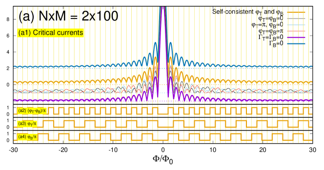
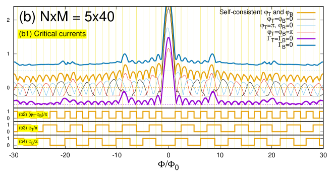
Figure 2: The numerical results. The critical currents are shown as a function of the reduced magnetic flux, for the self-consistent solution (bold orange lines), and for the nonself-consistent $\varphi_{T}=\varphi_{B}=0$ (thin black lines) and $\varphi_{T}=\pi$, $\varphi_{B}=0$ (light blue lines). The thick magenta lines correspond to absence of coupling to the superconducting leads $S_{T}$ and $S_{B}$ on top and bottom, i.e. to a two-terminal Josephson junction with $\Sigma^{(1)}_{B}=\Sigma^{(1)}_{T}=0$. The thick blue lines show a three-terminal Josephson junction having an additional superconducting mirror, with $\Sigma^{(1)}_{B}=0$. Panels a2, a3 and a4 show the self-consistent $(\varphi_{T}-\varphi_{B})/\pi$, $\varphi_{T}/\pi$ and $\varphi_{B}/\pi$ respectively with two superconducting mirrors. We use $\Sigma_{0}=10$ for the bulk hopping amplitude in $N_{0}$, $\Gamma_{L}=\Gamma_{R}=\Gamma_{T}=\Gamma_{B}\equiv\Gamma$ with $\Gamma=1$ for the contact transparencies and $W_{g}=0.4$ for the value of the gate voltage. The supercurrents are in units of $2e\Gamma/\hbar$. We also use $N\times M=2\times 100$ (panel a) and $N\times M=5\times 40$ (panel b).

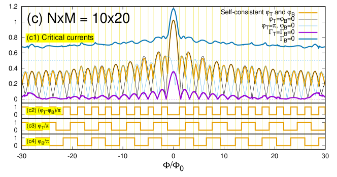
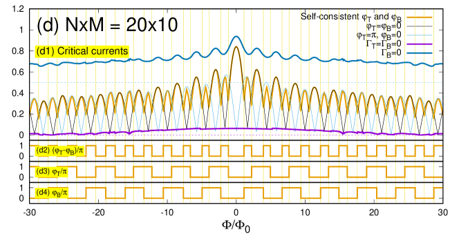
Figure 3: The same as Fig. 2 but now with $N\times M=10\times 20$ (panel c) and $N\times M=20\times 10$ (panel d).

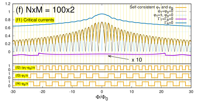
Figure 4: The same as Fig. 2 but in addition, the thin red lines correspond to $\varphi_{T}=\varphi_{B}=\pi$. We use $N\times M=40\times 5$ (panel e) and $N\times M=100\times 2$ (panel f).

II.4 Algorithm

The numerical calculations proceed with exact diagonalizations of the large-gap Hamiltonian defined in the above subsections II.1, II.2 and II.3. The supercurrents are obtained from the derivative of the ground state energy with respect to the superconducting phase variables. We denote by ${\cal E}_{0}\left(B,\varphi_{1},\,...,\,\varphi_{n}\right)$ the ground state energy:

$${\cal E}_{0}\left(B,\varphi_{1},\,...,\,\varphi_{n}\right)=$$ (62)

$$\sum_{\alpha}\epsilon_{\alpha}\left(B,\varphi_{1},\,...,\,\varphi_{n}\right)\theta\left[-\epsilon_{\alpha}\left(B,\varphi_{1},\,...,\,\varphi_{n}\right)\right],$$

where the ABS have the energies $\epsilon_{\alpha}\left(B,\varphi_{1},\,...,\,\varphi_{n}\right)$ and the Heaviside $\theta$-function selects negative energies in the zero-temperature limit. The current through lead $S_{p}$ is then given by

$$I_{S_{p}}\left(B,\varphi_{1},\,...,\,\varphi_{n}\right)=-\frac{2e}{\hbar}\frac{\partial{\cal E}_{0}}{\partial\varphi_{p}}\left(B,\varphi_{1},\,...,\,\varphi_{n}\right).$$ (63)

III Results

In this section, we present and physically discuss the numerical results obtained from the superconducting tight-binding model presented in the above Sec. II. Our main numerical results are presented in Fig. 2a, Fig. 2b, Fig. 3c, Fig. 3d and Fig. 4e, Fig. 4f, corresponding to the full range of the aspect ratios. The corresponding device dimensions are $N\times M=2\times 100,\,5\times 40,\,10\times 20,\,20\times 10,\,40\times 5$ and $100\times 2$ respectively, with the fixed overall tight-binding lattice area ${\cal S}=200\,a_{0}^{2}$. The devices geometry ranges from being elongated in the vertical to horizontal directions. The presentation of the results may look unusual in the sense that the discussion in the text proceeds with two terminals, next two terminals plus a single superconducting mirror and finally two terminals plus two superconducting mirrors, thus not consisting in a discussion of the figures one after the other.

Concerning the devices containing a single or two superconducting mirrors, considerable gains in the computation times are obtained if all of the superconducting leads $S_{L}$, $S_{R}$, $S_{T}$ and $S_{B}$ are coupled to the normal-metallic conductor $N_{0}$ by symmetric hopping amplitudes, see Appendix A. This symmetry condition is fulfilled by the identical hopping amplitudes implemented in our calculations.

After recovering known behavior with two terminals, the numerical results with superconducting mirrors will next be presented and discussed. The supercurrent flowing between the left and right superconductors $S_{L}$ and $S_{R}$ in the horizontal direction will be enhanced by orders of magnitudes in the presence of the single superconducting mirror $S_{T}$. With the two superconducting mirrors $S_{T}$ and $S_{B}$, we will obtain an oscillatory critical current magnetic pattern that resembles the oscillations of a SQUID, due to the interfering supercurrent paths through the top and bottom superconductors $S_{T}$ and $S_{B}$.

Two terminals: Now, we proceed with discussing the numerical results in themselves, starting with two terminals as a point of comparison for testing the large-gap calculations. We first consider a device where the two superconducting leads $S_{L}$ and $S_{R}$ are connected to the left and right, without the superconducting mirror $S_{T}$ and $S_{B}$, neither on top nor on bottom (see Figs. 1a and 1b). The numerical data with two terminals are shown with the bold magenta lines labeled by $\Gamma_{T}=\Gamma_{B}=0$ on panels a1-f1 of Fig. 2 to Fig. 4.

Figs. 2a, Fig. 2b and Fig. 3c correspond to $N\times M=2\times 100$, $N\times M=5\times 40$ and $N\times M=10\times 20$ respectively. We then obtain the expected Fraunhofer-like oscillation pattern for those devices elongated along the $y$-axis direction.

Next, the two-terminal critical current is negligibly small if the device is elongated along the $x$-axis direction, see the bold magenta lines labeled by $\Gamma_{T}=\Gamma_{B}=0$ in Fig. 4e and Fig. 4f with $N\times M=40\times 5$ and $N\times M=100\times 2$ respectively.

We also find quasimonotonous decay of the critical current as a function of the magnetic field if the device dimension in the horizontal direction is reduced according to $N\times M=20\times 10$, see the bold magenta line on Fig. 3d. We carried out complementary calculations of the ABS spectrum, revealing that the small “jumps” appearing in the datapoints represented by the bold magenta lines in Fig. 3d signal that some ABS cross the zero of energy as a function of the magnetic field.

The overall evolution from Fraunhofer pattern to quasimonotonous decay of the critical current flowing from $S_{L}$ to $S_{R}$ is in a qualitative agreement with a preceding work on disordered superconductor-normal metal-superconductor junctions in a field, see Ref. Cuevas2007, . Now that we demonstrated consistency with known results, we further proceed with three- and four-terminal devices containing a single or two superconducting mirrors respectively.

A single superconducting mirror: Now, we consider that a third superconducting lead $S_{T}$ is connected on top to the rectangular normal-metallic conductor $N_{0}$, see Fig. 1c. We calculate the maximal value of the supercurrent flowing between $S_{L}$ and $S_{R}$ connected to the left and right edges respectively. As discussed above, $S_{T}$ on top is an open-circuit superconducting mirror and the overall supercurrent transmitted into $S_{T}$ is vanishingly small. However, $S_{T}$ can propagate supercurrent in the direction parallel to its interface with $N_{0}$.

The corresponding data for the critical current in the presence of this third superconducting mirror $S_{T}$ laterally connected on top are shown by the dark blue lines labeled by $\Gamma_{B}=0$ in all Fig. 2-a1 to Fig. 4-f1. Those datapoints are vertically shifted according to the reference represented by the horizontal blue dashed lines.

Devices elongated in the vertical direction produce oscillations in the critical current as a function of the applied magnetic field, see the dark blue lines in Fig. 2-a1 to Fig. 3-d1 corresponding to $N\times M=2\times 100,\,5\times 40,\,10\times 20,\,20\times 10$ respectively. We note that, for those device dimensions, the ratio between the critical currents at the central peak and at the first lobe is anomalously large in comparison with the standard Fraunhofer pattern Tinkham . Given the intermediate contact transparencies in our calculations, we possibly relate this zero-field anomaly to the constructive interference of reflectionless tunneling at low magnetic field, see Ref. Schechter2001, .

The corresponding critical currents flowing between the left and right superconductors $S_{L}$ and $S_{R}$ in the horizontal direction are shown by the dark blue lines labeled by $\Gamma_{B}=0$ on panels e1-f1 of Fig. 4, for $N\times M=40\times 5$ and $N\times M=100\times 2$. Those values are enhanced by orders or magnitude in comparison with a two-terminal device (i.e. with $\Gamma_{T}=\Gamma_{B}=0$ in the absence of the coupling to $S_{T}$). This enhancement is interpreted as phase rigidity in the superconductor mirror $S_{T}$ connected on top. Namely, propagating supercurrent from $S_{L}$ to $S_{R}$ in the horizontal direction involves supercurrent lines connecting $S_{L}$ to $S_{T}$, followed by propagation over arbitrary long distances inside the rigid condensate of $S_{T}$, and finally the supercurrent lines are transmitted from $S_{T}$ to $S_{R}$.

Two superconducting mirrors: We now consider the four-terminal Josephson device with two superconducting mirrors, where the supercurrent in the horizontal direction flows between the two superconductors $S_{L}$ and $S_{R}$ connected to the left and right edges of the rectangular normal-metallic $N_{0}$, in the presence of the two superconducting mirrors $S_{T}$ and $S_{B}$ laterally connected on top and bottom, see Fig. 1d and Fig. 1e.

Panels a1-f1 of Fig. 2, Fig. 3 and Fig. 4 show the critical currents as a function of the magnetic field, with self-consistent superconducting phase variables (see the bold orange lines labeled by “Self-consistent $\varphi_{T}$ and $\varphi_{B}$”). The self-consistent solution minimizes the ground state energy ${\cal E}_{0}$ with respect to the superconducting phase variables $\varphi_{T},\,\varphi_{B}=0$ or $\pi$ according to Appendix A, see also Eq. (62) for the expression of the ground state energy ${\cal E}_{0}$.

As for a single superconducting mirror $S_{T}$, we observe that connecting the two superconducting mirrors $S_{T}$ and $S_{B}$ on top and bottom produces an enhancement of the critical current flowing between the left and right superconductors $S_{L}$ and $S_{R}$ in the horizontal direction, see Fig. 4a and Fig. 4b for $N\times M=40\times 5$ and $N\times M=100\times 2$ respectively. The supercurrent from $S_{L}$ and $S_{R}$ or from $S_{R}$ to $S_{L}$ in the horizontal direction can be viewed as being guided by the superconducting mirrors $S_{T}$ and $S_{B}$ on top and bottom.

The critical current magnetic oscillations resemble those of a SQUID, due to the interference between the Cooper pairs traveling in the superconducting leads $S_{T}$ and $S_{B}$ on top and bottom respectively.

The thinner black lines labeled by $\varphi_{T}=\varphi_{B}=0$ in Fig. 2a, Fig. 2b, Fig. 3c, Fig. 3d, Fig. 4e and Fig. 4f show the critical current with the nonself-consistent $\varphi_{T}=\varphi_{B}=0$, and the thinner light-blue lines labeled by “$\varphi_{T}=\pi,\,\varphi_{B}=0$” correspond to the nonself-consistent $\varphi_{T}=\pi$ and $\varphi_{B}=0$. The light-red lines labeled by “$\varphi_{T}=\varphi_{B}=\pi$” in Fig. 2a and Fig. 2b correspond to $\varphi_{T}=\varphi_{B}=\pi$. We conclude that the critical current calculated with the self-consistent $\varphi_{T}$ and $\varphi_{B}$ (see the bold orange lines labeled by “Self-consistent $\varphi_{T}$ and $\varphi_{B}$”) switches between those nonself-consistent solutions as the magnetic field is increased.

Fig. 2-a2 to Fig. 4-f2 show the normalized difference $(\varphi_{T}-\varphi_{B})/\pi$ between the self-consistent phase variables $\varphi_{T}$ and $\varphi_{B}$ of the superconducting mirrors. Fig. 2-a3 to Fig. 4-f3 and Fig. 2-a4 to Fig. 4-f4 show the normalized self-consistent $\varphi_{T}/\pi$ and $\varphi_{B}/\pi$ respectively. Remarkably, all minima in the critical current pattern on panels a1-f1 correlate with the magnetic field values at which $(\varphi_{T}-\varphi_{B})/\pi$ switches between zero and unity or vice-versa. The thin vertical yellow lines across each Fig. 2 to Fig. 4 match all of those switching points in $(\varphi_{T}-\varphi_{B})/\pi$.

We conclude that, in the limit of a device elongated in the horizontal direction, (i.e. with $N\gg M$), the magnetic field-dependence of the critical current is controlled by $(\varphi_{T}-\varphi_{B})/\pi$, instead of each $\varphi_{T}/\pi$ or $\varphi_{B}/\pi$ taken individually. In the opposite limit of a device elongated in the vertical direction (i.e. if $M\gg N$), the superconducting phase variables $\varphi_{T}$ and $\varphi_{B}$ of $S_{T}$ and $S_{B}$ are spectators. Their values is driven by the supercurrent flowing between $S_{L}$ and $S_{R}$ in the horizontal direction. In addition, Fig. 2a and Fig. 2b feature the magnetic flux dependence of the nonself-consistent $\varphi_{T}=\varphi_{B}=\pi$, which strongly deviates from the nonself-consistent $\varphi_{T}=\varphi_{B}=0$.

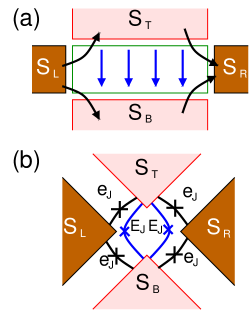
Figure 5: The four superconducting leads $S_{L}$, $S_{R}$, $S_{T}$ and $S_{B}$ on the left, right, top and bottom (a) are transformed into the phenomenological Josephson junction circuit model (b). The neighboring superconducting leads are connected by small Josephson coupling $e_{J}$ and the top and bottom ones $S_{T}$ and $S_{B}$ are connected by two Josephson junctions with large Josephson coupling $E_{J}$, reflecting the corresponding large-area contacts between $S_{T}$ and $S_{B}$ through the normal metal ${N_{0}}$.

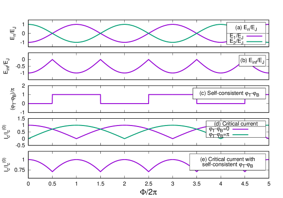
Figure 6: The figure illustrates the phenomenological Josephson junction circuit model calculation. The figure shows the energies $E_{1}$ and $E_{2}$ as a function of $\Phi/2\pi$ [see Eq. (66)] (a), the ground state energy $E_{inf}=\inf(E_{1},E_{2})$ between the lowest between $E_{1}$ and $E_{2}$ (b), the normalized self-consistent $(\varphi_{T}-\varphi_{B})/2\pi$ (c), the nonself-consistent critical currents $I_{c}$ for $\varphi_{T}-\varphi_{B}=0$ and $\varphi_{T}-\varphi_{B}=\pi$ (d), and the critical current $I_{c}$ with the self-consistent $\varphi_{T}-\varphi_{B}$ (e).

IV Phenomenological Josephson junction circuit model

In this section, we propose a phenomenological Josephson junction circuit model suitable to geometries elongated in the horizontal direction, i.e. with $N\gg M$. The Josephson coupling energy $E_{J}$ between the top and bottom superconductors $S_{T}$ and $S_{B}$ is large, due to the corresponding large area interfaces. The Josephson coupling energies $e_{J}$ between the pairs $(S_{B},\,S_{L})$, $(S_{L},\,S_{T})$, $(S_{T},\,S_{R})$ and $(S_{R},\,S_{B})$ is smaller, see Fig. 5. This simple model relies on a few weak links and it is thus not intended to capture the zero-field anomaly appearing in the above numerical calculations.

The total energy takes the form

$$E = -E_{J}\cos\left(\varphi_{T}-\varphi_{B}+\frac{\Phi}{2\Phi_{0}}\right)$$

$$-E_{J}\cos\left(\varphi_{T}-\varphi_{B}-\frac{\Phi}{2\Phi_{0}}\right)$$

$$-e_{J}\cos\left(\varphi_{T}-\varphi_{L}+\frac{\Phi}{4\Phi_{0}}\right)-e_{J}\cos\left(\varphi_{L}-\varphi_{B}+\frac{\Phi}{4\Phi_{0}}\right)$$

$$-e_{J}\cos\left(\varphi_{B}-\varphi_{R}+\frac{\Phi}{4\Phi_{0}}\right)-e_{J}\cos\left(\varphi_{R}-\varphi_{T}+\frac{\Phi}{4\Phi_{0}}\right).$$

Assuming $E_{J}\gg e_{J}$, the supercurrent entering $S_{T}$ is approximated as

$$-\frac{2e}{\hbar}\frac{\partial E}{\partial\varphi_{T}} \simeq \frac{2e}{\hbar}E_{J}\sin\left(\varphi_{T}-\varphi_{B}+\frac{\Phi}{2\Phi_{0}}\right)$$

$$+ \frac{2e}{\hbar}E_{J}\sin\left(\varphi_{T}-\varphi_{B}-\frac{\Phi}{2\Phi_{0}}\right).$$

Injecting $\varphi_{T}-\varphi_{B}=0$ or $\pi$ into Eq. (IV) leads to the zero-current condition $-(2e/\hbar)\partial E/\partial\varphi_{T}=0$, with the corresponding energies $E_{1}$ and $E_{2}$

$$E_{1}=-2E_{J}\cos\left(\frac{\Phi}{2\Phi_{0}}\right)\equiv-E_{2}$$ (66)

associated to $\varphi_{T}-\varphi_{B}=0$ and $\varphi_{T}-\varphi_{B}=\pi$ respectively. As the normalized magnetic flux $\Phi/\Phi_{0}$ increases, the ground state energy alternates between $E_{1}$ and $E_{2}$ in Eq. (66), corresponding to locking the phases $\varphi_{T}$ and $\varphi_{B}$ according to $\varphi_{T}-\varphi_{B}=0$ or $\varphi_{T}-\varphi_{B}=\pi$ respectively. For instance, $\varphi_{T}-\varphi_{B}=0$ and $\varphi_{T}-\varphi_{B}=\pi$ are obtained in the intervals $|\Phi/2\Phi_{0}|<\pi/2$ and $\pi/2<|\Phi/2\Phi_{0}|<3\pi/2$ respectively.

Fig. 6a to Fig. 6c illustrate the flux-sensitivity of $E_{1},\,E_{2}$ in Eq. (66) (panel a), the ground state energy $E_{inf}=\inf(E_{1},\,E_{2})$ (panel b) and the self-consistent $\varphi_{T}-\varphi_{B}$ (panel c). Comments on panels d and e are provided below.

Now, we successively evaluate the supercurrents for $\varphi_{T}-\varphi_{B}=0$ and $\varphi_{T}-\varphi_{B}=\pi$. First considering $\varphi_{T}=\varphi_{B}=0$ leads to the following expression of the $\varphi_{L}$- and $\varphi_{R}$-sensitive energy terms $E_{L}$ and $E_{R}$:

$$E_{L}(\varphi_{L},\Phi)$$ (67)

$$= -e_{J}\cos\left(-\varphi_{L}+\frac{\Phi}{4\Phi_{0}}\right)-e_{J}\cos\left(\varphi_{L}+\frac{\Phi}{4\Phi_{0}}\right)$$

$$= -2e_{J}\cos\varphi_{L}\cos\left(\frac{\Phi}{4\Phi_{0}}\right)$$

$$E_{R}(\varphi_{R},\Phi)$$

$$= -e_{J}\cos\left(-\varphi_{R}+\frac{\Phi}{4\Phi_{0}}\right)-e_{J}\cos\left(\varphi_{R}+\frac{\Phi}{4\Phi_{0}}\right)$$ (69)

$$= -2e_{J}\cos\varphi_{R}\cos\left(\frac{\Phi}{4\Phi_{0}}\right).$$ (70)

We obtain

$$I_{L}(\varphi_{L},\Phi) = -\frac{2e}{\hbar}\frac{\partial E_{L}}{\partial\varphi_{L}}(\varphi_{L},\Phi)$$ (71)

$$= -\frac{4e}{\hbar}e_{J}\sin\varphi_{L}\cos\left(\frac{\Phi}{4\Phi_{0}}\right)$$ (72)

$$I_{R}(\varphi_{R},\Phi) = -\frac{2e}{\hbar}\frac{\partial E_{R}}{\partial\varphi_{R}}(\varphi_{R},\Phi)$$ (73)

$$= -\frac{4e}{\hbar}e_{J}\sin\varphi_{R}\cos\left(\frac{\Phi}{4\Phi_{0}}\right).$$ (74)

The condition $I_{R}+I_{L}=0$ leads to $\sin\varphi_{L}=-\sin\varphi_{R}$, and to $\varphi_{R}=-\varphi_{L}$ or $\varphi_{R}=\varphi_{L}+\pi$. We observe that $E_{L}(\varphi_{L},\Phi)+E_{R}(\varphi_{L}+\pi,\Phi)=0$, and we can always find values of $\varphi_{L}$ having the lower energy $E_{L}(\varphi_{L},\Phi)+E_{R}(-\varphi_{L},\Phi)<0$, which is why we restrict to $\varphi_{R}=-\varphi_{L}\equiv\psi$. It turns out that the ground state energy is negative for all values of the reduced magnetic flux $\Phi/\Phi_{0}$, see Fig. 6b.

Assuming now $\varphi_{T}=0$ and $\varphi_{B}=\pi$, we obtain

$$E^{\prime}_{L}(\varphi_{L},\Phi)$$ (75)

$$= -e_{J}\cos\left(-\varphi_{L}+\frac{\Phi}{4\Phi_{0}}\right)+e_{J}\cos\left(\varphi_{L}+\frac{\Phi}{4\Phi_{0}}\right)$$

$$= -2e_{J}\sin\varphi_{L}\sin\left(\frac{\Phi}{4\Phi_{0}}\right)$$

$$E^{\prime}_{R}(\varphi_{R},\Phi)$$

$$= e_{J}\cos\left(-\varphi_{R}+\frac{\Phi}{4\Phi_{0}}\right)-e_{J}\cos\left(\varphi_{R}+\frac{\Phi}{4\Phi_{0}}\right)$$ (77)

$$= 2e_{J}\sin\varphi_{R}\sin\left(\frac{\Phi}{4\Phi_{0}}\right),$$ (78)

and

$$I^{\prime}_{L}(\varphi_{L},\Phi) = -\frac{2e}{\hbar}\frac{\partial E^{\prime}_{L}}{\partial\varphi_{L}}(\varphi_{L},\Phi)$$ (79)

$$= \frac{4e}{\hbar}e_{J}\cos\varphi_{L}\sin\left(\frac{\Phi}{4\Phi_{0}}\right)$$ (80)

$$I^{\prime}_{R}(\varphi_{R},\Phi) = -\frac{2e}{\hbar}\frac{\partial E^{\prime}_{R}}{\partial\varphi_{R}}(\varphi_{R},\Phi)$$ (81)

$$= -\frac{4e}{\hbar}e_{J}\cos\varphi_{R}\sin\left(\frac{\Phi}{4\Phi_{0}}\right),$$ (82)

where, again, we used $\varphi_{R}=-\varphi_{L}\equiv\psi$.

Fig. 6d shows the critical current as a function of the normalized magnetic flux for the nonself-consistent solutions with $\varphi_{T}-\varphi_{B}=0$ and $\varphi_{T}-\varphi_{B}=\pi$. Fig. 6e shows the value of the supercurrent calculated with the self-consistent $\varphi_{T}-\varphi_{B}$, which amounts to taking the maximum between the two values on Fig. 6d. We note consistency with the preceding numerical calculations presented in Fig. 2 to Fig. 4, see the above Sec. III.

Finally, we have four phase variables $\varphi_{L},\,\varphi_{R},\,\varphi_{T}$ and $\varphi_{B}$. The constraint $\varphi_{R}=-\varphi_{L}\equiv\psi$ originates from the external current source which imposes opposite supercurrents transmitted into $S_{L}$ and $S_{R}$, therefore defining a net current flowing from $S_{L}$ to $S_{R}$ or from $S_{R}$ to $S_{L}$ in the horizontal direction. Those opposite supercurrents $I_{R}=-I_{L}$ couple to the remaining phase combinations $\varphi_{T}-\varphi_{B}=0$ or $\pi$ and $\varphi_{R}=-\varphi_{L}\equiv\psi$, where $\varphi_{B}$ is left undetermined. This is compatible with gauge invariance where one of those superconducting phase variables cannot be fixed. We conclude that, in the long-junction limit, the supercurrent flowing from $S_{L}$ to $S_{R}$ or from $S_{R}$ to $S_{L}$ in the horizontal direction couples to all possibly allowed phase combinations, as it is already the case in the short-junction limit.

V Conclusions

To conclude, we considered a multiterminal Josephson junction circuit model with the four superconducting leads $S_{L}$, $S_{R}$, $S_{T}$ and $S_{B}$ connected to the left, right, top and bottom edges of a normal-metallic rectangle $N_{0}$.

Concerning three terminals, we demonstrated that, for devices elongated in the horizontal direction, attaching the superconducting mirror $S_{T}$ on top of the normal conductor $N_{0}$ enhances the horizontal supercurrent by orders of magnitude, as a result of phase rigidity in the open-circuit superconductor $S_{T}$.

Concerning four terminals, we calculated the supercurrent flowing from $S_{L}$ to $S_{R}$ in the horizontal direction in the presence of the two superconducting mirrors $S_{T}$ and $S_{B}$, and we obtained oscillatory magnetic oscillations reminiscent of a SQUID. Those oscillations are controlled by the self-consistent phase variables $\varphi_{T}$ and $\varphi_{B}$ of the superconductors $S_{T}$ and $S_{B}$ connected on top and bottom respectively.

If the hopping amplitudes connecting the ballistic rectangular normal-metallic conductor $N_{0}$ to the superconductors are symmetric, then $\varphi_{T}$ and $\varphi_{B}$ take the values $0$ or $\pi$, as for an emerging Ising degree of freedom.

We also interpreted our numerical results with a simple Josephson junction circuit model, and demonstrated that the supercurrent flows through all parts of the circuit if the device is elongated in the horizontal direction.

In the numerical calculations and in the phenomenological circuit model, the horizontal supercurrent was controlled by the difference $\varphi_{T}-\varphi_{B}=0$ or $\pi$ instead of each individual $\varphi_{T}$ or $\varphi_{B}$, thus providing sensitivity to a single effective Ising degree of freedom of the supercurrent flowing in the horizontal direction.

Finally, a recent experimental work Pankratova2020 measured the critical current contours (CCCs) in the plane of the two biasing currents $I_{1}$ and $I_{2}$. The zero-current conditions $I_{1}=0$ or $I_{2}=0$ are fulfilled at the points where the CCCs intersect the $x$- or $y$-current axis respectively. Thus, our theory of the phase rigidity is expected to produce specific signatures on the CCCs, which will be the subject of a future work.

Appendix A Symmetries

In this Appendix, we show how the symmetries considerably reduce the computation times if the current flowing from $S_{L}$ to $S_{R}$ in the horizontal direction is specifically evaluated. Namely, we demonstrate that the following symmetries:

$$\varphi_{T},\,\varphi_{B}=0\mbox{ or }\pi\mbox{, and }\varphi_{L}=-\varphi_{R}\equiv\psi$$ (83)

are equivalent to vanishingly small supercurrent transmitted into the top and bottom superconductors $S_{T}$ and $S_{B}$, i.e. (83) implies that $S_{T}$ and $S_{B}$ are superconducting mirrors. The condition (83) also implies that opposite supercurrents are transmitted into $S_{L}$ and $S_{R}$ connected on the left and right edges of the rectangular normal-metallic conductor $N_{0}$. Conservation of the supercurrent between $S_{L}$ and $S_{R}$ in the horizontal direction is thus automatically fulfilled. Now, we demonstrate those statements.

Eqs. (58)-(59) become

$$\Gamma_{loc}^{(Left)}(y) = -\frac{(\Sigma^{(1)})^{2}}{W}e^{i\varphi_{L}^{(0)}}e^{iBLy/2\Phi^{\prime}_{0}}e^{2iBya_{0}/\Phi^{\prime}_{0}}$$ (84)

$$\Gamma_{loc}^{(Right)}(y) = -\frac{(\Sigma^{(1)})^{2}}{W}e^{i\varphi_{R}^{(0)}}e^{-iBLy/2\Phi^{\prime}_{0}}e^{-2iBya_{0}/\Phi^{\prime}_{0}},$$ (85)

where we use the notation $x_{R/L}=\pm L/2$. We obtain

$$\Gamma_{loc}^{(Left)}(y)=\left(\Gamma_{loc}^{(Right)}\right)^{*}(y)$$ (86)

if $e^{i\varphi_{L}^{(0)}}=e^{-i\varphi_{R}^{(0)}}$, i.e. if $\varphi_{L}=-\varphi_{R}\equiv\psi$, see the condition (83).

Conversely, the substitution $x\rightarrow\overset{\sim}{{x}}=-x$ leads to $\Gamma_{loc}^{(Top)}\rightarrow\overset{\sim}{{\Gamma}}_{loc}^{(Top)}$ and $\Gamma_{loc}^{(Bottom)}\rightarrow\overset{\sim}{{\Gamma}}_{loc}^{(Bottom)}$ in Eqs. (60)-(61), with

$$\overset{\sim}{{\Gamma}}_{loc}^{(Top)}(x) = -\frac{(\Sigma^{(1)})^{2}}{W}e^{i\varphi_{T}^{(0)}}e^{-iBWx/2\Phi^{\prime}_{0}}e^{-2iBxa_{0}/\Phi^{\prime}_{0}}$$ (87)

$$\overset{\sim}{{\Gamma}}_{loc}^{(Bottom)}(x) = -\frac{(\Sigma^{(1)})^{2}}{W}e^{i\varphi_{B}^{(0)}}e^{iBWx/2\Phi^{\prime}_{0}}e^{2iBxa_{0}/\Phi^{\prime}_{0}},$$ (88)

where we used the notation $y_{T,B}=\pm W/2$.

We deduce the following:

$$\overset{\sim}{{\Gamma}}_{loc}^{(Top)} = \left({\Gamma}_{loc}^{(Top)}\right)^{*}$$ (89)

$$\overset{\sim}{{\Gamma}}_{loc}^{(Bottom)} = \left({\Gamma}_{loc}^{(Bottom)}\right)^{*}$$ (90)

if both $e^{i\varphi_{B}^{(0)}}$ and $e^{i\varphi_{T}^{(0)}}$ are real-valued, i.e. if $\varphi_{B}^{(0)},\,\varphi_{T}^{(0)}=0$ or $\pi$, see the condition (83).

Now, we discuss the consequences for the supercurrents flowing across the normal-metallic conductor $N_{0}$. At the lowest order in tunneling, the typical combinations

$$\Gamma_{loc}^{(Left)}(y)\left({\Gamma}_{loc}^{(Bottom)}(x)\right)^{*}$$ (91)

and

$$\Gamma_{loc}^{(Right)}(y)\left({\Gamma}_{loc}^{(Bottom)}(x)\right)^{*}$$ (92)

control the DC-Josephson effect between the left/bottom and the right/bottom superconducting leads. The following identity:

$$\Gamma_{loc}^{(Left)}(y)\left({\Gamma}_{loc}^{(Bottom)}(x)\right)^{*}$$

$$= \left[\Gamma_{loc}^{(Right)}(y)\left({\Gamma}_{loc}^{(Bottom)}(-x)\right)^{*}\right]^{*}$$

leads to opposite values for the supercurrents transmitted from left to bottom and from right to bottom if the condition (83) is fulfilled, since the corresponding superconducting phase differences are opposite.

We conclude that the mirror-axis symmetry $x\rightarrow\overset{\sim}{{x}}=-x$ leads to vanishingly small value for the sum $I_{L\rightarrow B}+I_{R\rightarrow B}$ of the supercurrents $I_{L\rightarrow B}$ (from left to bottom) and $I_{R\rightarrow B}$ (from right to bottom), i.e. $I_{L\rightarrow B}+I_{R\rightarrow B}=0$. Similarly, we find $I_{L\rightarrow T}+I_{R\rightarrow T}=0$ for the sum of the supercurrents from left to top and from right to top.

Using the form of the Bethe-Salpeter equations suitable to Andreev tubes (see for instance Refs.Kraft2018, ; Meier2016, for the Andreev tubes), this perturbative argument can be extended to all orders in the tunneling amplitudes $\Sigma^{(1)}$ connecting the normal region ${N_{0}}$ to each of the superconducting leads, see Eq. (5) for the notation $\Sigma^{(1)}$.

In Sec. III of the main text, the three- and four-terminal calculations with a single or two superconducting mirrors respectively are realized with identical value for all of the tunneling amplitudes between the normal region $N_{0}$ and the superconductors. The symmetry condition (83) is then automatically fulfilled and the energy minimum is within the discrete set $\varphi_{T},\,\varphi_{B}=0$ or $\pi$. Scanning those restricted values of $\varphi_{T}$ and $\varphi_{B}$ (as it was the case in the above Sec. III) allows for considerable gain in the computation time with respect to looking for the energy minimum in the entire $\left[0,\,2\pi\right]\times\left[0,\,2\pi\right]$ intervals.

References

- (1) R. de Bruyn Ouboter and A. Omelyanchouk, Multi-terminal squid controlled by the transport current, Physica B: Condensed Matter 205, 153 (1995).
- (2) M. Amin, A. Omelyanchouk, and A. Zagoskin, Mesoscopic multiterminal Josephson structures. i. effects of nonlocal weak coupling, Low Temperature Physics 27, 616 (2001).
- (3) M. Amin, A. Omelyanchouk, and A. Zagoskin, Dc squid based on the mesoscopic multiterminal Josephson junction, Physica C: Superconductivity 372, 178 (2002).
- (4) M. Amin, A. Omelyanchouk, A. Blais, A. M. van den Brink, G. Rose, T. Duty, and A. Zagoskin, Multi-terminal superconducting phase qubit, Physica C: Superconductivity 368, 310 (2002).
- (5) A. Freyn, B. Douçot, D. Feinberg, and R. Mélin, Production of non-local quartets and phase-sensitive entanglement in a superconducting beam splitter, Phys. Rev. Lett. 106, 257005 (2011).
- (6) R. Mélin, D. Feinberg, and B. Douçot, Partially resummed perturbation theory for multiple Andreev reflections in a short three-terminal Josephson junction, Eur. Phys. J. B 89, 67 (2016).
- (7) T. Jonckheere, J. Rech, T. Martin, B. Douçot, D. Feinberg, and R. Mélin, Multipair DC Josephson resonances in a biased allsuperconducting bijunction, Phys. Rev. B 87, 214501 (2013).
- (8) R. Mélin, Inversion in a four terminal superconducting device on the quartet line. I. Two-dimensional metal and the quartet beam splitter, Phys. Rev. B 102, 245435 (2020).
- (9) R. Mélin and B. Douçot, Inversion in a four terminal superconducting device on the quartet line. II. Quantum dot and Floquet theory, Phys. Rev. B 102, 245436 (2020).
- (10) R. Mélin and D. Feinberg, Quantum interferometer for quartets in superconducting three-terminal Josephson junctions, Phys. Rev. B 107, L161405 (2023).
- (11) R. Mélin, R. Danneau and C.B. Winkelmann, Proposal for detecting the -shifted Cooper quartet supercurrent, Phys. Rev. Res. 5, 033124 (2023).
- (12) R. Mélin, J.-G. Caputo, K. Yang and B. Douçot, Simple Floquet-Wannier-Stark-Andreev viewpoint and emergence of low-energy scales in a voltage-biased three-terminal Josephson junction, Phys. Rev. B 95, 085415 (2017).
- (13) R. Mélin, R. Danneau, K. Yang, J.-G. Caputo, and B. Douçot, Melin2019 the Floquet spectrum of superconducting multiterminal quantum dots, Phys. Rev. B 100, 035450 (2019).
- (14) B. Douçot, R. Danneau, K. Yang, J.-G. Caputo and R. Mélin, Berry phase in superconducting multiterminal quantum dots, Phys. Rev. B 101, 035411 (2020).
- (15) R. Mélin, Ultralong-distance quantum correlations in three-terminal Josephson junctions, Phys. Rev. B 104, 075402 (2021).
- (16) R. Mélin, Multiterminal ballistic Josephson junctions coupled to normal leads, Phys. Rev. B 105, 155418 (2022).
- (17) A. Keliri and B. Douçot, Driven Andreev molecule, Phys. Rev. B 107, 094505 (2023); A. Keliri and B. Douçot, Long-range coupling between superconducting dots induced by periodic driving, arXiv:2304.05987 (2023).
- (18) R.-P. Riwar, M. Houzet, J.S. Meyer, and Y.V. Nazarov, Multi-terminal Josephson junctions as topological materials, Nat. Commun. 7, 11167 (2016).
- (19) E. Eriksson, R.-P. Riwar, M. Houzet, J. S. Meyer, and Y. V. Nazarov, Topological transconductance quantization in a four-terminal Josephson junction, Phys. Rev. B 95, 075417 (2017).
- (20) H.-Y. Xie, M.G. Vavilov and A. Levchenko, Topological Andreev bands in three-terminal Josephson junctions, Phys. Rev. B 96, 161406 (2017).
- (21) H.-Y. Xie, M.G. Vavilov and A. Levchenko, Weyl nodes in Andreev spectra of multiterminal Josephson junctions: Chern numbers, conductances and supercurrents, Phys. Rev. B 97, 035443 (2018).
- (22) O. Deb, K. Sengupta and D. Sen, Josephson junctions of multiple superconducting wires, Phys. Rev. B 97, 174518 (2018).
- (23) B. Venitucci, D. Feinberg, R. Mélin, B. Douçot, Nonadiabatic Josephson current pumping by microwave irradiation, Phys. Rev. B 97, 195423 (2018).
- (24) L.P. Gavensky, G. Usaj, D. Feinberg and C.A. Balseiro, Berry curvature tomography and realization of topological Haldane model in driven three-terminal Josephson junctions, Phys. Rev. B 97, 220505 (2018).
- (25) R. L. Klees, G. Rastelli, J. C. Cuevas, and W. Belzig, Microwave Spectroscopy Reveals the Quantum Geometric Tensor of Topological Josephson Matter, Phys. Rev. Lett. 124, 197002 (2020).
- (26) V. Fatemi, A.R. Akhmerov and L. Bretheau, Weyl Josepshon circuits, Phys. Rev. Research 3, 013288 (2021).
- (27) L. Peyruchat, J. Griesmar, J.-D. Pillet and Ç.Ö Girit, Transconductance quantization in a topological Josephson tunnel junction circuit, Phys. Rev. Research 3, 013289 (2021).
- (28) H. Weisbrich, R.L. Klees, G. Rastelli and W. Belzig, Second Chern Number and Non-Abelian Berry Phase in Topological Superconducting Systems, PRX Quantum 2, 010310 (2021).
- (29) Y. Chen and Y.V. Nazarov, Weyl point immersed in a continuous spectrum: an example from superconducting nanostructures, Phys. Rev. B 104, 104506 (2021).
- (30) Y. Chen and Y.V. Nazarov, Spin-Weyl quantum unit: theoretical proposal, Phys. Rev. B 103, 045410 (2021).
- (31) E.V. Repin and Y.V. Nazarov, Weyl points in the multi-terminal Hybrid Superconductor-Semiconductor Nanowire devices, Phys. Rev. B 105, L041405 (2022).
- (32) L. Peralta Gavensky, G. Usaj and C.A. Balseiro, Multiterminal Josephson junctions: a road to topological flux networks, Europhys. Lett. 141 36001 (2023).
- (33) J.D. Pillet, V. Benzoni, J. Griesmar, J.-L. Smirr, and Ç.Ö. Girit, Nonlocal Josephson effect in Andreev molecules Nano Lett. 19, 7138 (2019).
- (34) J.-D. Pillet, V. Benzoni, J. Griesmar, J.-L. Smirr, and Ç. Ö. Girit, Scattering description of Andreev molecules, SciPost Phys. Core 2, 009 (2020).
- (35) V. Kornich, H.S. Barakov, and Yu.V. Nazarov, Fine energy splitting of overlapping Andreev bound states in multiterminal superconducting nanostructures, Phys. Rev. Research 1, 033004 (2019).
- (36) J. -D. Pillet, S. Annabi, A. Peugeot, H. Riechert, E. Arrighi, J. Griesmar, L. Bretheau, Josephson Diode Effect in Andreev Molecules, Phys. Rev. Res. 5, 033199 (2023).
- (37) A.H. Pfeffer, J.E. Duvauchelle, H. Courtois, R. Mélin, D. Feinberg, and F. Lefloch, Subgap structure in the conductance of a three-terminal Josephson junction, Phys. Rev. B 90, 075401 (2014).
- (38) Y. Cohen, Y. Ronen, J.H. Kang, M. Heiblum, D. Feinberg, R. Mélin, and H. Strikman, Non-local supercurrent of quartets in a three-terminal Josephson junction, Proc. Natl. Acad. Sci. U.S.A. 115, 6991 (2018).
- (39) K.F. Huang, Y. Ronen, R. Mélin, D. Feinberg, K. Watanabe, T. Taniguchi, and P. Kim, Evidence for 4e charge of Cooper quartets in a biased multi-terminal graphene-based Josephson junction, Nat. Comm. 13, 3032 (2022).
- (40) G. V. Graziano, M. Gupta, M. Pendharkar, J. T. Dong, C. P. Dempsey, C. Palmstrøm and V. S. Pribiag, Selective control of conductance modes in multi-terminal Josephson junctions, Nat. Comm. 13, 5933 (2022).
- (41) S. Park, W. Lee, S. Jang, Y.-B. Choi, J. Park, W. Jung, K. Watanabe, T. Taniguchi, G. Y. Cho and G.-H. Lee, Steady Floquet-Andreev states in graphene Josephson junctions, Nature 603, 421 (2022).
- (42) O. Kürtössy, Z. Scherübl, G. Fülöp, I. E. Lukács, T. Kanne, J. Nygard, P. Makk and S. Csonka, Andreev molecule in parallel InAs nanowires, Nano Lett. 21, 7929 (2021).
- (43) M. Coraiola, D. Z. Haxell, D. Sabonis, H. Weisbrich, A. E. Svetogorov, M. Hinderling, S. C. ten Kate, E. Cheah, F. Krizek, R. Schott, W. Wegscheider, J. C. Cuevas, W. Belzig, and F. Nichele, Hybridisation of Andreev bound states in three-terminal Josephson junctions, Nat. Commun. 14, 6784 (2023).
- (44) S. Matsuo, T. Imoto, T. Yokoyama, Y. Sato, T. Lindemann, S. Gronin, G. C. Gardner, S. Nakosai, Y. Tanaka, M. J. Manfra, and S. Tarucha, Phase-dependent Andreev molecules and superconducting gap closing in coherently coupled Josephson junctions, arXiv:2303.10540 (2023).
- (45) S. Matsuo, T. Imoto, T. Yokoyama, Y. Sato, T. Lindemann, S. Gronin, G. C. Gardner, M. J. Manfra, and S. Tarucha, Engineering of anomalous Josephson effect in coherently coupled Josephson junctions, arXiv:2305.06596 (2023).
- (46) M. Gupta, G. V. Graziano, M. Pendharkar, J. T. Dong, C. P. Dempsey, C. Palmstrøm and V. S. Pribiag, Superconducting diode effect in a three-terminal Josephson device, Nat. Commun. 14, 3078 (2023).
- (47) F. Zhang, M. T. Ahari, A. S. Rashid, G. J. de Coster, T. Taniguchi, K. Watanabe, M. J. Gilbert, N. Samarth and M. Kayyalha, Reconfigurable magnetic-field-free superconducting diode effect in multi-terminal Josephson junctions, arXiv:2301.05081 (2023).
- (48) A.W. Draelos, M.-T. Wei, A. Seredinski, H. Li, Y. Mehta, K. Watanabe, T. Taniguchi, I.V. Borzenets, F. Amet, and G. Finkelstein, Supercurrent flow in multiterminal graphene Josephson junctions, Nano Lett. 19, 1039 (2019).
- (49) N. Pankratova, H. Lee, R. Kuzmin, K. Wickramasinghe, W. Mayer,J. Yuan,M. Vavilov,J. Shabani and V. Manucharyan, The multi-terminal Josephson effect, Phys. Rev. X 10, 031051 (2020).
- (50) G.V. Graziano, J.S. Lee, M. Pendharkar, C. Palmstrøm and V.S. Pribiag, Transport studies in a gate-tunable three-terminal Josephson junction, Phys. Rev. B 101, 054510 (2020).
- (51) E.G. Arnault, T. Larson, A. Seredinski, L. Zhao, H. Li, K. Watanabe, T. Taniguchi, I. Borzenets, F. Amet and G. Finkelstein, The multiterminal inverse AC Josephson effect, Nano Lett. 21, 9668 (2021).
- (52) S.A. Khan, L. Stampfer, T. Mutas, J.-H. Kang, P. Krogstrup and T.S. Jespersen, Multiterminal Quantized Conductance in InSb Nanocrosses, Advanced Materials 33, 2100078 (2021).
- (53) E.G. Arnault, S. Idris, A. McConnell, L. Zhao, T.F.Q. Larson, K. Watanabe, T. Taniguchi, G. Finkelstein, F. Amet, Dynamical stabilization of multiplet supercurrents in multi-terminal Josephson junctions, Nano Lett. 22, 7073 (2022).
- (54) S. Matsuo, J.S. Lee, C.-Y. Chang, Y. Sato, K. Ueda, C.J. Palstrøm and S. Tarucha, Observation of the nonlocal Josephson effect on double InAs nanowires, Communications Physics 5, 221 (2022).
- (55) F. Zhang, A.S. Rashid, M.T. Ahari, W. Zhang, K.M. Ananthanarayanan, R. Xiao, G.J. de Coster, M.J. Gilbert, N. Samarth and M. Kayyalha, Andreev processes in mesoscopic multi-terminal graphene Josephson junctions, Phys. Rev. B 107, L140503 (2023).
- (56) J.M. Rowell, Magnetic field dependence of the Josephson tunnel current, Phys. Rev. Lett. 11, 200 (1963).
- (57) R.C. Dynes and T.A. Fulton, Supercurrent density distribution in Josephson junctions Phys. Rev. B 3, 3015 (1971).
- (58) H.H. Zappe, Determination of the current density distribution in Josephson tunnel junctions. Phys. Rev. B 7, 2535 (1975).
- (59) A. Barone, and G. Paterno, Physics and Applications of the Josephson Effect (John Wiley, 1982).
- (60) M. Tinkham, Introduction to Superconductivity, 2nd ed. (McGraw-Hill, New York, 1996).
- (61) V. Barzykin, and A.M. Zagoskin, Coherent transport and nonlocality in mesoscopic SNS junctions: anomalous magnetic interference patterns, Superlatt. Microstruct. 25, 797 (1999).
- (62) K. Kikuchi, H. Myoren, T. Iizuka, and S. Takada, Normal-distribution function- shaped Josephson tunnel junctions. Appl. Phys. Lett. 77, 3660 (2000).
- (63) L. Angers, F. Chiodi, G. Montambaux, M. Ferrier, S. Guéron, H. Bouchiat, and J.C. Cuevas, Proximity dc squids in the long-junction limit. Phys. Rev. B 77, 165408 (2008).
- (64) F. Chiodi, M. Ferrier, S. Guéron, J.C. Cuevas, G. Montambaux, F. Fortuna, A. Kasumov, and H. Bouchiat, Geometry-related magnetic interference patterns in long SNS Josephson junctions. Phys. Rev. B 86, 064510 (2012).
- (65) M. Amado, A. Fornieri, F. Carillo, G. Biasiol, L. Sorba, V. Pellegrini, and F. Giazotto, Electrostatic tailoring of magnetic interference in quantum point contact ballistic Josephson junctions, Phys. Rev. B 87, 134506 (2013).
- (66) S. Hart, H. Ren, T. Wagner, P. Leubner, M. Mühlbauer, C. Brüne, H. Buhmann, L.W. Molenkamp, and A. Yacoby, Induced superconductivity in the quantum spin Hall edge. Nature Phys. 10, 638 (2014).
- (67) M.T. Allen, O. Shtanko, I.C. Fulga, A.R. Akhmerov, K. Watanabe, T. Taniguchi, P. Jarillo-Herrero, L.S. Levitov, and A.Yacoby, Spatially resolved edge currents and guided-wave electronic states in graphene. Nature Phys. 12, 128 (2016).
- (68) F. Amet, C.T. Ke, I.V. Borzenets, J.J. Wang, K. Watanabe, T. Taniguchi, R.S. Deacon, M. Yamamoto, Y. Bomze, S. Tarucha, and G. Finkelstein, Supercurrent in the quantum Hall regime. Science 352, 966 (2016).
- (69) H. Meier, V.I. Fal’ko and L. Glazman, Edge effects in the magnetic interference pattern of a ballistic SNS junction, Phys. Rev. B 93, 184506 (2016).
- (70) R. Kraft, J. Mohrmann, R. Du, P. B. Selvasundaram, M. Irfan, U. Nefta Kanilmaz, F. Wu, D. Beckmann, H. v. Löhneysen, R. Krupke, A. Akhmerov, I. Gornyi, and R. Danneau, Tailoring supercurrent confinement in graphene bilayer weak links, Nat. Commun. 9, 1722 (2018).
- (71) M. Irfan, and A.R. Akhmerov, Geometric focusing of supercurrent in hourglass-shaped ballistic Josephson junctions, arXiv:1810.04588 (2018).
- (72) P. Pandey, D. Beckmann and R. Danneau, Energy distribution controlled ballistic Josephson junction, Phys. Rev. B 106, 214503 (2022).
- (73) C.-G. Chu, J.-J. Chen, A.-Q. Wang, Z.-B. Tan, C.-Z. Li, C. Li, A. Brinkman, P.-Z. Xiang, . Li, Z.-C. Pan, H.-Z. Lu, D. Yu, and Z.-M. Liao, Broad and colossal edge supercurrent in Dirac semimetal Cd3As2 Josephson junctions, Nat. Commun. 14, 6162 (2023).
- (74) A. Melo, V. Fatemi and A.R. Akhmerov, Multiplet supercurrent in Josephson tunneling circuits, SciPost Phys. 12, 017 (2022).
- (75) A. Zazunov, V. S. Shumeiko, E. N. Bratus’, J. Lantz, and G. Wendin, Andreev Level Qubit, Phys. Rev. Lett. 90, 087003 (2003).
- (76) T. Meng, S. Florens and P. Simon, Self-consistent description of Andreev bound states in Josephson quantum dot devices, Phys. Rev. B 79, 224521 (2009).
- (77) S.B. Kaplan, C.C. Chi, D.N. Langenberg, J.J. Chang, S. Jafarey, and D.J. Scalapino, Quasiparticle and phonon lifetimes in superconductors, Phys. Rev. B 14, 4854 (1976).
- (78) R.C. Dynes, V. Narayanamurti, and J.P. Garno, Direct measurement of quasiparticle-lifetime broadening in a strong-coupled superconductor, Phys. Rev. Lett. 41, 1509 (1978).
- (79) J.P. Pekola, V.F. Maisi, S. Kafanov, N. Chekurov, A. Kemppinen, Yu.A. Pashkin, O.-P. Saira, M. Möttönen, and J.S. Tsai, Environment-assisted tunneling as an origin of the Dynes density of states, Phys. Rev. Lett. 105, 026803 (2010).
- (80) O.-P. Saira, A. Kemppinen, V.F. Maisi, and J.P. Pekola, Vanishing quasiparticle density in a hybrid Al/Cu/Al single-electron transistor, Phys. Rev. B 85, 012504 (2012).
- (81) J.C. Cuevas, A. Martín-Rodero, and A. Levy Yeyati, Hamiltonian approach to the transport properties of superconducting quantum point contacts, Phys. Rev. B 54, 7366 (1996).
- (82) J.C. Cuevas and F.S. Bergeret, Magnetic Interference Patterns and Vortices in Diffusive SNS Junctions, Phys. Rev. Lett. 99, 217002 (2007).
- (83) M. Schechter, Y. Imry and Y. Levinson, Reflectionless tunneling in ballistic normal-metal–superconductor junctions Phys. Rev. B 64, 224513 (2001).