Modeling Complex Disease Trajectories using Deep Generative Models with Semi-Supervised Latent Processes

Abstract

In this paper, we propose a deep generative time series approach using latent temporal processes for modeling and holistically analyzing complex disease trajectories. We aim to find meaningful temporal latent representations of an underlying generative process that explain the observed disease trajectories in an interpretable and comprehensive way. To enhance the interpretability of these latent temporal processes, we develop a semi-supervised approach for disentangling the latent space using established medical concepts. By combining the generative approach with medical knowledge, we leverage the ability to discover novel aspects of the disease while integrating medical concepts into the model.

We show that the learned temporal latent processes can be utilized for further data analysis and clinical hypothesis testing, including finding similar patients and clustering the disease into new sub-types. Moreover, our method enables personalized online monitoring and prediction of multivariate time series including uncertainty quantification. We demonstrate the effectiveness of our approach in modeling systemic sclerosis, showcasing the potential of our machine learning model to capture complex disease trajectories and acquire new medical knowledge.

1 Introduction

Understanding and analyzing clinical trajectories of complex diseases - such as systemic sclerosis - is crucial for improving diagnosis, treatment, and patient outcomes. However, modeling such multivariate time series data poses significant challenges due to the high dimensionality of clinical measurements, low signal-to-noise ratio, sparsity, and the complex interplay of various - potentially unobserved - factors influencing the disease progression.
 
Therefore, our primary goal is to develop a machine learning (ML) model suited for the holistic analysis of temporal disease trajectories. Moreover, we aim to uncover meaningful temporal latent representations capturing the complex interactions within the raw data while also providing interpretable insights, and potentially revealing novel medical aspects of clinical disease trajectories.
 
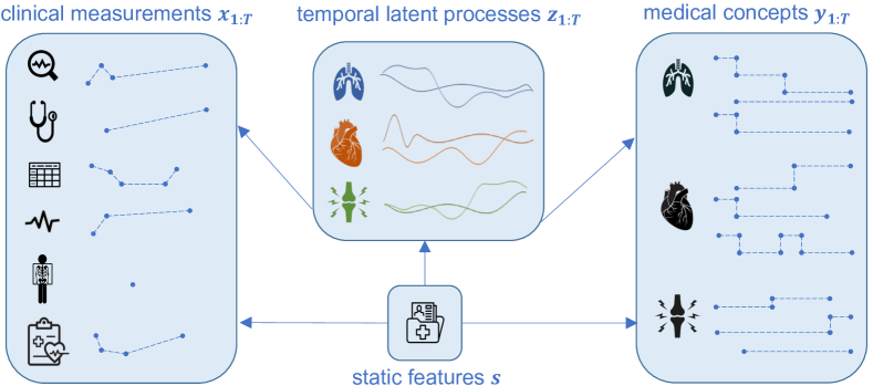
To achieve these goals, we present a deep generative temporal model that captures both the joint distribution of all the observed longitudinal clinical variables and of the latent temporal variables (LABEL:fig:overview). Since inferring interpretable temporal representations in a fully unsupervised way is very challenging (Locatello et al., 2020a), we propose a semi-supervised approach for disentangling the latent space using known medical concepts to enhance the interpretability. Combining an unsupervised latent generative model with known medical labels allows for the discovery of novel medically-driven patterns in the data.
 
Deep probabilistic generative models (Appendix E and Tomczak (2022)) provide a more holistic approach to modeling complex data than deterministic discriminative models. By learning the joint distribution over all involved variables, they model the underlying generating mechanism. In contrast, discriminative models only learn the conditional distribution of the target variable given the input variables.
 
While our method is general and can be applied to a wide range of high-dimensional clinical datasets, in this paper, we demonstrate its effectiveness in modeling the progression of systemic sclerosis (SSc), a severe and yet only partially understood autoimmune disease. SSc triggers the immune system to attack the body’s connective tissue, causing severe damage to the skin and multiple other internal organs. We seek to understand the evolution of SSc by modeling the patterns of organ involvement and progression. In doing so, we aim to learn temporal hidden representations that distinctly capture the disentangled medical concepts related to each organ.

fig:overview

Figure 1: Temporal generative model for systemic sclerosis.

Our approach offers several contributions:

• Interpretable Temporal Latent Process: Our generative model allows the non-linear projection of patient trajectories onto a lower-dimensional temporal latent process, providing useful representations for visualization and understanding of complex medical time series data.

• Semi-Supervised Guided Latent Process: To achieve more interpretable latent temporal spaces, we propose a semi-supervised approach for disentangling the latent space by leveraging known medical concepts. By combining the generative approach with medical domain knowledge, new aspects of the disease can be discovered.

• Online Prediction with Uncertainty: Our deep generative probabilistic model facilitates personalized online monitoring and robust/reliable prediction of multivariate time series data using uncertainty quantification.

• Facilitating Clinical Hypothesis Testing: The learned temporal latent processes can be inspected for further data analysis and clinical hypothesis testing, such as finding similar patients and clustering the disease trajectories into new sub-types.

• Large-Scale Analysis of SSc : We demonstrate the potential of our ML model for comprehensively analyzing SSc for the first time at a large scale including multiple organs and various observed clinical variables.

2 Background

2.1 Generative Latent Variable Models

Learning latent representations from raw data has a long tradition in statistics and ML with foundational research such as principal component analysis (Hotelling, 1933), factor analysis (Lawley and Maxwell, 1962) or independent component analysis (Comon, 1994), which all can be used to project high-dimensional tabular data to a latent space. For temporal data, models with latent processes such as hidden Markov models (Baum and Petrie, 1966) and Gaussian processes (Williams and Rasmussen, 2006) have extensively been used for discrete and continuous time applications, respectively. Conceptually, all these models can be interpreted as probabilistic generative models with latent variables (e.g. Murphy (2022)), however only exploiting linear or simple mappings from the original to the latent space.

In their seminal work on Variational Autoencoders (VAEs), Kingma and Welling (2013) proposed a powerful generalization for latent generative models. The key idea is to use deep neural networks as powerful function approximators to learn the moments of the distributions in the generative probabilistic model, enabling the representation of arbitrarily complex distributions. Inference for the parameters of the neural networks is done with amortized variational inference (VI) (Blei et al., 2017), a powerful approximate Bayesian inference tool. There are various successors building and improving on the original model, for instance, conditional VAE (Sohn et al., 2015), LVAE (Sønderby et al., 2016), or VQ-VAE (Van Den Oord et al., 2017). Moreover, there are also several extensions that explicitly model time in the latent space such as RNN-VAE (Chung et al., 2015), GP-VAE (Casale et al., 2018; Fortuin et al., 2020), or longitudinal VAE (Ramchandran et al., 2021).

While these approaches have showcased remarkable efficacy in generating diverse objects such as images or modeling time series, the interpretability of the resulting latent spaces or processes remains limited for complex data. Moreover, the true underlying concepts for known processes often cannot be recovered, and instead become entangled within a single latent factor (Bengio et al., 2013). Thus, there is ongoing research in designing generative models with disentangled latent factors, such as $\beta-$VAE (Higgins et al., 2016), factorVAE (Kim and Mnih, 2018), TCVAE (Chen et al., 2018) or temporal versions including disentangled sequential VAE (Hsu et al., 2017) and disentangled GP-VAE (Bing et al., 2021).

However, learning interpretable and disentangled latent representations is highly difficult or even impossible for complex data without any inductive bias (Locatello et al., 2020a). Hence, purely unsupervised modeling falls short, leading researchers to focus on weakly supervised latent representation learning instead (Locatello et al., 2020b; Zhu et al., 2022; Palumbo et al., 2023).

In a similar spirit, we tackle the temporal semi-supervised guidance of the latent space by providing sparse labels representing established medical domain knowledge concepts. We model the progression of complex diseases in an unsupervised way using the raw clinical measurements, while also including medical temporal concept labels.

2.2 Analyzing Disease Trajectories with ML

Recently, extensive research has focused on modeling and analyzing clinical time series with machine learning – we refer to Allam et al. (2021) for a recent overview. However, most approaches focus on deterministic time series forecasting, and only a few focus on interpretable representation learning with deep models (Trottet et al., 2023) and irregularly sampled times (Chen et al., 2023) or on online uncertainty quantification with generative models (Schürch et al., 2020; Cheng et al., 2020; Rosnati and Fortuin, 2021).

Furthermore, prior research on data-driven analysis of systemic sclerosis is limited. In their recent review, Bonomi et al. (2022) discuss the existing studies applying machine learning for precision medicine in systemic sclerosis. However, all of the listed studies are limited by the small cohort size (maximum of 250 patients), making the use of deep learning models challenging. Deep models were only used for analyzing imaging data (mainly nailfold capillaroscopy, Garaiman et al. (2022)). Furthermore, most existing works solely focus on the involvement of a single organ in SSc, namely interstitial lung disease (ILD), and on forecasting methods. To the best of our knowledge, our work is the first attempt at such a comprehensive and large-scale (N=5673 patients) ML analysis of systemic sclerosis involving multiple organs and a wide range of observed clinical variables together with a systematic integration of medical knowledge.

3 Methodology

We analyze patient histories that consist of two main types of data: raw temporal clinical measurements $\boldsymbol{x}=\boldsymbol{x}_{1:T}\in\mathbb{R}^{D\times T}$, such as blood pressure, and sparse medical concept labels $\boldsymbol{y}=\boldsymbol{y}_{1:T}\in\mathbb{R}^{P\times T}$, describing higher-level medical definitions related to the disease, for instance, the medical definition of severity staging of the heart involvement (LABEL:fig:overview). The medical concept definitions are typically derived from multiple clinical measurements using logical operations. For example, a patient may be classified as having “severe heart involvement” if certain conditions are satisfied, for instance, $\boldsymbol{x}^{(i)}>\varepsilon$ AND $\boldsymbol{x}^{(j)}=1$. Both the raw measurements and labels are irregularly sampled, and we denote by $\boldsymbol{\tau}_{1:T}\in\mathbb{R}^{T}$ the vector of sampling time-points. Moreover, static information denoted as $\boldsymbol{s}\in\mathbb{R}^{S}$ is present, alongside additional temporal covariates such as medications $\boldsymbol{p}_{1:T}\in\mathbb{R}^{P\times T}$ for each patient.

We condition our generative model on the context variable $\boldsymbol{c}=\{\boldsymbol{\tau},\boldsymbol{p},\boldsymbol{s}\}$ to be able to generate latent processes under certain conditions, for instance when a specific medication is administered. Furthermore, in the next sections, we introduce our approach to learning multivariate latent processes denoted as $\boldsymbol{z}=\boldsymbol{z}_{1:T}\in\mathbb{R}^{L\times T}$, responsible for generating both the raw clinical measurement processes $\boldsymbol{x}_{1:T}$ and the medical labels $\boldsymbol{y}_{1:T}$. In particular, we use the different temporal medical concepts to disentangle the $L$ dimensions of the latent processes by allocating distinct dimensions to represent different medical concepts.

We assume a dataset $\{\boldsymbol{x}^{i}_{1:T_{i}},\boldsymbol{y}^{i}_{1:T_{i}},\boldsymbol{c}^{i}_{1:T_{i}}\}_{i=1}^{N}$ of $N$ patients, and omit the dependency to $i$ and the time index when the context is clear. Note that the measurements and medical concepts are often partially observed, see more details in Appendix B.1.1.

3.1 Generative Model

We propose the probabilistic conditional generative latent variable model

$$p_{\psi}(\boldsymbol{y},\boldsymbol{x},\boldsymbol{z}|\boldsymbol{c})=p_{\gamma}(\boldsymbol{y}|\boldsymbol{z},\boldsymbol{c})p_{\pi}(\boldsymbol{x}|\boldsymbol{z},\boldsymbol{c})p_{\phi}(\boldsymbol{z}|\boldsymbol{c}),$$

with learnable prior network $p_{\phi}(\boldsymbol{z}|\boldsymbol{c})$, measurement likelihood network $p_{\pi}(\boldsymbol{x}|\boldsymbol{z},\boldsymbol{c})$, and guidance network $p_{\gamma}(\boldsymbol{y}|\boldsymbol{z},\boldsymbol{c})$, where $\psi=\{\gamma,\pi,\phi\}$ are learnable parameters. For the sake of brevity, we do not include the time index explicitly. Although the measurements and the concepts are conditionally independent given the latent variables, the marginal distribution $p_{\psi}(\boldsymbol{y},\boldsymbol{x}|\boldsymbol{c})=\int p_{\psi}(\boldsymbol{y},\boldsymbol{x},\boldsymbol{z}|\boldsymbol{c})d\boldsymbol{z}$ allows arbitrarily rich correlations among the observed variables.

3.2 Prior of Latent Process

We use a learnable prior network for the latent temporal variables $\boldsymbol{z}$, that is,

$$p_{\phi}(\boldsymbol{z}|\boldsymbol{c}) =\prod_{t=1}^{T}\prod_{l=1}^{L}\mathcal{N}\left(\boldsymbol{z}_{t}^{l}|\mu_{\phi}^{l}(\boldsymbol{c}_{t}),\sigma^{l}_{\phi}(\boldsymbol{c}_{t})\right),$$

conditioned on the context variables $\boldsymbol{c}=\{\boldsymbol{\tau},\boldsymbol{p},\boldsymbol{s}\}$, so that time-varying or demographic effects can be learned in the prior (Appendix D.2.1). The means $\mu_{\phi}^{l}(\boldsymbol{c}_{t})$ and variances $\sigma^{l}_{\phi}(\boldsymbol{c}_{t})$ are learnable deep neural networks. We assume a factorized Gaussian prior distribution per time and latent dimensions, however, many interesting extensions including continuous-time priors are straightforward (Appendix B.2).

fig:model

Figure 2: Semi-supervised temporal latent variable model with generative and inference model.

3.3 Likelihood of Measurements

The probabilistic likelihood network maps the latent temporal processes $\boldsymbol{z}\in\mathbb{R}^{L\times T}$ together with the context variables $\boldsymbol{c}$ to the clinical measurements $\boldsymbol{x}\in\mathbb{R}^{D\times T}$, i.e.

$$p_{\pi}(\boldsymbol{x}|\boldsymbol{z},\boldsymbol{c}) =\prod_{t=1}^{T}\prod_{d\in\mathcal{G}}\mathcal{N}(x_{t}^{d}|\mu_{\pi}^{d},\sigma^{d}_{\pi})\prod_{d\in\mathcal{K}}\mathcal{C}(x_{t}^{d}|p_{\pi}^{d}),$$

where we assume time- and feature-wise conditional independence. We assume either Gaussian $\mathcal{N}$ or categorical $\mathcal{C}$ likelihoods for the observed variables $\boldsymbol{x}$, where $\mathcal{G}$ and $\mathcal{K}$ are the corresponding indices. The moments of these distributions are deep parametrized functions, i.e. for the mean $\mu_{\pi}^{d}=\mu_{\pi}^{d}(\boldsymbol{z}_{t},\boldsymbol{c}_{t})$, variance $\sigma^{d}_{\pi}=\sigma^{d}_{\pi}(\boldsymbol{z}_{t},\boldsymbol{c}_{t})$, and category probability vector $p_{\pi}^{d}=p_{\pi}^{d}(\boldsymbol{z}_{t},\boldsymbol{c}_{t})$. Although the likelihood is a parametric distribution, we want to emphasize that the posterior distribution can be arbitrarily complex after marginalizing out the latent process $\boldsymbol{z}$.

3.4 Semi-Supervised Guidance Network

We propose a semi-supervised approach to disentangle the latent process $\boldsymbol{z}$ with respect to defined medical concepts $\boldsymbol{y}=\boldsymbol{y}_{1:T}\in\mathbb{R}^{P\times T}$. In particular, we assume

$$p_{\gamma}(\boldsymbol{y}|\boldsymbol{z},\boldsymbol{c}) =\prod_{t=1}^{T}\prod_{g=1}^{G}\prod_{j\in\nu(g)}\mathcal{C}(y_{t}^{j}|h_{\gamma}^{j}(\boldsymbol{z}_{t}^{\varepsilon(g)},\boldsymbol{c}_{t})),$$

where $h_{\gamma}^{j}(\boldsymbol{z}_{t}^{\varepsilon(g)},\boldsymbol{c}_{t})$ is a deep parametrized probability vector, and $\nu(g)$ and $\varepsilon(g)$ correspond to the indices of the $g$th guided medical concept, and the indices in the latent space defined for guided concept $g$, respectively.

3.5 Posterior of Latent Process

We are mainly interested in the posterior distribution $p_{\psi}(\boldsymbol{z}|\boldsymbol{x},\boldsymbol{y},\boldsymbol{c})$ of the latent process given the observations, which we approximate with an amortized variational distribution (Section 3.6, Appendix B.1)

$$q_{\theta}(\boldsymbol{z}|\boldsymbol{x},\boldsymbol{c})\approx p_{\psi}(\boldsymbol{z}|\boldsymbol{x},\boldsymbol{y},\boldsymbol{c}).$$

In particular, we use the amortized variational distribution

$$q_{\theta}(\boldsymbol{z}|\boldsymbol{x}_{0:k},\boldsymbol{c}) =\prod_{t=1}^{T}\prod_{l=1}^{L}\mathcal{N}(z_{t}^{l}|\mu_{\theta}^{l}(\boldsymbol{x}_{0:k},\boldsymbol{c}),\sigma^{l}_{\theta}(\boldsymbol{x}_{0:k},\boldsymbol{c}))$$

with variational parameters $\theta$ and $0\leq k\leq T$. Note that only the measurements $\boldsymbol{x}_{0:k}$ until observation $k$ are part of the variational distribution, and not the medical concepts $\boldsymbol{y}$. If $k=T$, there is no forecasting, whereas for $0\leq k<T$, we can also forecast the future latent variables $\boldsymbol{z}_{k+1:T}$ from the first measurements $\boldsymbol{x}_{0:k}$.

3.6 Probabilistic Inference

Since exact inference with the marginal likelihood $p_{\psi}(\boldsymbol{x},\boldsymbol{y}|\boldsymbol{c})=\int p_{\gamma}(\boldsymbol{y}|\boldsymbol{z},\boldsymbol{c})p_{\pi}(\boldsymbol{x}|\boldsymbol{z},\boldsymbol{c})p_{\phi}(\boldsymbol{z}|\boldsymbol{c})d\boldsymbol{z}$ is not feasible (Appendix B.1), we apply amortized variational inference (Blei et al., 2017) by maximizing a lower bound $\log p_{\psi}(\boldsymbol{x},\boldsymbol{y}|\boldsymbol{c})\geq\mathcal{L}(\psi,\theta;\boldsymbol{x},\boldsymbol{y},\boldsymbol{c})$ of the intractable marginal log likelihood. For a fixed $k$, this leads to the following objective function

$$\begin{split}\mathcal{L}_{k}(\psi,\theta;\boldsymbol{x},\boldsymbol{y},\boldsymbol{c})=&~{}\mathbb{E}_{q_{\theta}(\boldsymbol{z}|\boldsymbol{x}_{0:k},\boldsymbol{c})}\left[\log p_{\pi}(\boldsymbol{x}|\boldsymbol{z},\boldsymbol{c})\right]\\ +&~{}\alpha~{}\mathbb{E}_{q_{\theta}(\boldsymbol{z}|\boldsymbol{x}_{0:k},\boldsymbol{c})}\left[\log p_{\gamma}(\boldsymbol{y}|\boldsymbol{z},\boldsymbol{c})\right]\\ -&~{}\beta~{}KL\left[q_{\theta}(\boldsymbol{z}|\boldsymbol{x}_{0:k},\boldsymbol{c})~{}||~{}p_{\phi}(\boldsymbol{z}|\boldsymbol{c})\right],\end{split}$$

where we introduce weights $\alpha$ and $\beta$ inspired by the disentangled $\beta-$VAE (Higgins et al., 2016).

The first term $\mathbb{E}_{q_{\theta}(\boldsymbol{z}|\boldsymbol{x},\boldsymbol{c})}\left[\log p_{\pi}(\boldsymbol{x}|\boldsymbol{z},\boldsymbol{c})\right]$ is unsupervised, whereas the second $\alpha\mathbb{E}_{q_{\theta}(\boldsymbol{z}|\boldsymbol{x},\boldsymbol{c})}\left[\log p_{\gamma}(\boldsymbol{y}|\boldsymbol{z},\boldsymbol{c})\right]$ is supervised and $\beta KL\left[q_{\theta}(\boldsymbol{z}|\boldsymbol{x},\boldsymbol{c})||p_{\phi}(\boldsymbol{z}|\boldsymbol{c})\right]$ is a regularization term, ensuring that the posterior is close to the prior with respect to the Kullback-Leibler (KL) divergence. Since all dimensions in the latent space $\boldsymbol{z}$ are connected to all the measurements $\boldsymbol{x}$, all the potential correlations between clinically measured variables can be exploited in an unsupervised fashion while disentangling the latent variables using the guidance networks for $\boldsymbol{y}$. The expectation over the variational distribution $\mathbb{E}_{q_{\theta}(\boldsymbol{z}|\boldsymbol{x},\boldsymbol{c})}$ is approximated with a few Monte-Carlo samples (Appendix B.1).

Given a dataset with $N$ $\mathrm{iid}$ patients $\{\boldsymbol{x}_{1:T_{i}}^{i},\boldsymbol{y}_{1:T_{i}}^{i},\boldsymbol{c}_{1:T_{i}}^{i}\}_{i=1}^{N}$, the optimal parameters are given by

$$\psi^{*},\theta^{*}=\operatorname*{argmax}_{\psi,\theta}\sum_{i=1}^{N}\sum_{k=0}^{T_{i}}\mathcal{L}_{k}(\psi,\theta;\boldsymbol{x}^{i},\boldsymbol{y}^{i},\boldsymbol{c}^{i}),$$

which is computed with stochastic optimization using mini-batches of patients and different values of $k$ (Appendix B.1.2). Since real-world time series data often contains many missing values, the objective function can be adapted accordingly (Appendix B.1.1).

3.7 Online Prediction with Uncertainty

Our model can be used for online monitoring and continuous prediction of high-dimensional medical concepts and clinical measurement distributions based on an increasing number of available clinical observations $\boldsymbol{x}_{0:k}$ for $k=0,1,\ldots,T$. The distributions

$$q_{*}(\boldsymbol{y}|\boldsymbol{x}_{0:k},\boldsymbol{c}) =\int p_{\gamma^{*}}(\boldsymbol{y}|\boldsymbol{z},\boldsymbol{c})q_{\theta^{*}}(\boldsymbol{z}|\boldsymbol{x}_{0:k},\boldsymbol{c})d\boldsymbol{z}$$

$$q_{*}(\boldsymbol{x}|\boldsymbol{x}_{0:k},\boldsymbol{c}) =\int p_{\pi^{*}}(\boldsymbol{x}|\boldsymbol{z},\boldsymbol{c})q_{\theta^{*}}(\boldsymbol{z}|\boldsymbol{x}_{0:k},\boldsymbol{c})d\boldsymbol{z}$$

are approximated with a two-stage Monte-Carlo sampling (Appendix B.1.3).

The former can be used to automatically label and forecast the multiple medical concepts based on the raw and partially observed measurements, whereas the latter corresponds to the reconstruction and forecasting of partially observed trajectories. Note that these distributions represent a complex class of potentially multi-modal distributions.

3.8 Patient Similarity and Clustering

The learned posterior network $q_{\theta^{*}}(\boldsymbol{z}_{1:T}|\boldsymbol{x}_{1:T},\boldsymbol{c}_{1:T})$ can be used to map any observed patient trajectory $\mathcal{T}_{i}=\{\boldsymbol{x}_{1:T_{i}}^{i},\boldsymbol{c}_{1:T_{i}}^{i}\}$ to its latent trajectory

$$\mathcal{H}_{i}=h(\mathcal{T}_{i})=\mathbb{E}_{q_{\theta}(\boldsymbol{z}_{1:T_{i}}^{i}|\boldsymbol{x}_{1:T_{i}}^{i},\boldsymbol{c}_{1:T_{i}}^{i})}\left[\boldsymbol{z}_{1:T_{i}}^{i}\right]$$

by taking the mean of the latent process. These temporal latent trajectories $\{\mathcal{H}_{i}\}_{i=1}^{N}$ of the $N$ patients in the cohort are used to define a patient similarity over the partially observed and high-dimensional original disease trajectories $\{\mathcal{T}_{i}\}_{i=1}^{N}$. Through our semi-supervised generative approach, the latent trajectories effectively capture the important elements from $\boldsymbol{x}_{1:T_{i}}^{i}$ and $\boldsymbol{y}_{1:T_{i}}^{i}$, without explicitly depending on $\boldsymbol{y}_{1:T_{i}}^{i}$. Indeed, all the information related to the medical concepts is learned by $\theta$.

Since defining a patient similarity measure between two trajectories $\mathcal{T}_{i}$ and $\mathcal{T}_{j}$ in the original space is very challenging, due to the missingness and high dimensionality, we instead propose to define it in the latent space, setting

$$d_{\mathcal{T}}\left(\mathcal{T}_{i},\mathcal{T}_{j}\right)=d_{\mathcal{H}}\left(\mathcal{H}_{i},\mathcal{H}_{j}\right).$$

To measure the similarity $d_{\mathcal{H}}\left(\mathcal{H}_{i},\mathcal{H}_{j}\right)$ between latent trajectories, we employ the dynamic-time-warping (dtw) measure to account for the different lengths of the trajectories as well as the potentially misaligned disease progressions in time (Müller, 2007). We then utilize the similarity measure to cluster the disease trajectories and identify similar patient trajectories as discussed in Section 4.2.2.

3.9 Modeling Systemic Sclerosis

We aim to model the overall SSc disease trajectories as well as the distinct organ involvement trajectories for patients from the European Scleroderma Trials and Research (EUSTAR) database. We provide a description of the database in Appendix A.2.

As a proof of concept, we focus on the involvement of three important organs in SSc, namely the lung, heart, and joints (arthritis). Each organ has two related medical concepts: involvement and stage. Based upon the medical definitions provided in Appendix A.3, for each of the three organs $\mathcal{O}:=\{lung,heart,joints\}$, we created labels signaling the organ involvement (yes/no) and severity stage ($1-4$), respectively. We write $o(m)$, $m\in\{involvement,stage\}$, $o\in\mathcal{O}$ to refer to the corresponding medical concept for organ $o$. We project the $D=34$ and $P=11$ input features to a latent process $\boldsymbol{z}$ of dimension $L=21$. For each organ, we guide a distinct subset of $7$ latent processes (non-overlapping subsets), thus all of the dimensions in $\boldsymbol{z}$ are guided. Following the notations from 3.4, we assume

$$p_{\gamma}(\boldsymbol{y}|\boldsymbol{z},\boldsymbol{c}) =\prod_{t=1}^{T}\prod_{\begin{subarray}{c}o\in\mathcal{O}\end{subarray}}\prod_{\begin{subarray}{c}m\in\\ {\{inv},\\ {stage\}}\\ \end{subarray}}p_{\gamma}(\boldsymbol{y}_{t}^{\nu(o(m))}|\boldsymbol{z}_{t}^{\varepsilon(o(m))},\boldsymbol{c}_{t}).$$

3.10 Deep Probabilistic Networks

As shown in LABEL:fig:model, our model combines several deep probabilistic networks. For the posterior $q_{\theta}(\boldsymbol{z}|\boldsymbol{x}_{0:k},\boldsymbol{c})$, we implemented a temporal network with fully connected and LSTM layers (Hochreiter and Schmidhuber, 1997) and multilayer perceptrons for the prior $p_{\phi}(\boldsymbol{z}|\boldsymbol{c})$, guidance $p_{\gamma}(\boldsymbol{y}|\boldsymbol{z},\boldsymbol{c})$ and likelihood $p_{\pi}(\boldsymbol{x}|\boldsymbol{z},\boldsymbol{c})$ networks. Implementation details are provided in Appendix C.1.

By changing the configuration of our framework, we are able to recover well-established temporal latent variable models. For instance, if we discard the guidance networks, the model becomes similar to a deterministic RNN-AE, or probabilistic RNN-VAE if we learn the latent space distribution. Furthermore, the likelihood variance can either be learned, or kept constant as is common practice (Rybkin et al., 2021). We evaluated the predictive performance of the guided model in the probabilistic and deterministic settings, with or without learning the likelihood variance. Many further architectural choices could be explored, such as a temporal likelihood network or a GP prior, but they are beyond this paper’s scope.

4 Experiments and Results

In this section, we discuss and compare different settings of our model and present experimental results on the EUSTAR database.

4.1 Model Evaluation

When referring to the model output, we use the term “prediction” to encompass both current (reconstructed) and future values, and use the term “forecasting” specifically when addressing future values alone.

Our model learns the optimal parameters for the likelihood $p_{\pi}(\boldsymbol{x}|\boldsymbol{z},\boldsymbol{c})$ and guidance networks $p_{\gamma}(\boldsymbol{y}|\boldsymbol{z},\boldsymbol{c})$ and predicts the complete $\boldsymbol{x}$ and $\boldsymbol{y}$ trajectories. As described in subsection 3.10, we assessed the model’s predictive performance in probabilistic and deterministic settings, and with either learning the likelihood network variance $\sigma^{*}$ or setting $\sigma=1$.

fig:performance

Figure 3: Performance for $\boldsymbol{x}$ prediction.

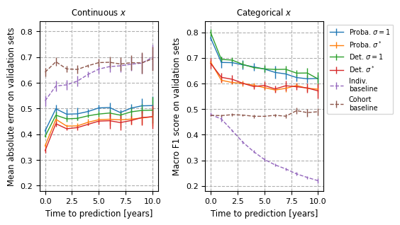
We used $5-$fold CV to select the hyperparameters that achieved the lowest validation loss. Details about the inference process are provided in subsection 3.6 and Appendix C.2.1.

LABEL:fig:performance shows the performance of predicting the clinical measurements $\boldsymbol{x}$. All of the models greatly outperform non-ML-driven individualized or cohort-based baselines. The individualized baseline predicts the patient’s last available measurement for a variable as its future value. The cohort baseline predicts a value sampled from the empirical Gaussian/Categorical distribution of the variable in the cohort. The models with learned $\sigma^{*}$ perform slightly better at predicting continuous $\boldsymbol{x}$ while enforcing $\sigma=1$ allows the models to better learn the categorical $\boldsymbol{x}$. The same holds for the prediction of the categorical medical concepts $\boldsymbol{y}$ (LABEL:fig:perf_y in the appendix). Furthermore, there is no significant decrease in performance in probabilistic versus deterministic settings, even though an additional regularization term is optimized (subsection 3.10). In Appendix D.1, we additionally compare the performance for $\boldsymbol{x}$ prediction of our guided model versus the optimal unguided baseline.

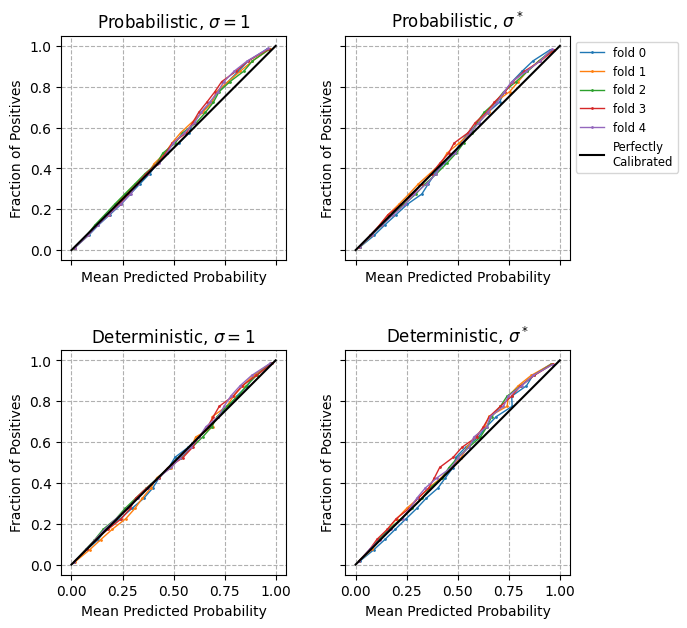
To evaluate the uncertainty quantification, we computed the coverage of the forecasted $95\%$ confidence intervals (CI) for continuous variables and the calibration for categorical variables. Further details are provided in Appendix D.1. For continuous $\boldsymbol{x}$ forecasting, both probabilistic models achieve coverage of $92\pm 1\%$ and of $98\pm 0\%$ for the deterministic models, thus all slightly diverging from the optimal $95\%$. All of the models have accurate calibration for categorical $\boldsymbol{x}$ and $\boldsymbol{y}$ forecasting (LABEL:fig:calib in the appendix).

The probabilistic model with learned $\sigma^{*}$ strikes the best balance between predictive capabilities, coverage and generative ability. In the next sections, we explore further applications and results of this final model. While the performance was computed on validation sets, the subsequent results are derived from applying the final model to a separate withheld test set. Furthermore, all of the $t-$SNE projections (Van der Maaten and Hinton, 2008) of the test set were obtained following the procedure described in Appendix D.2.2.

4.1.1 Online Prediction with Uncertainty

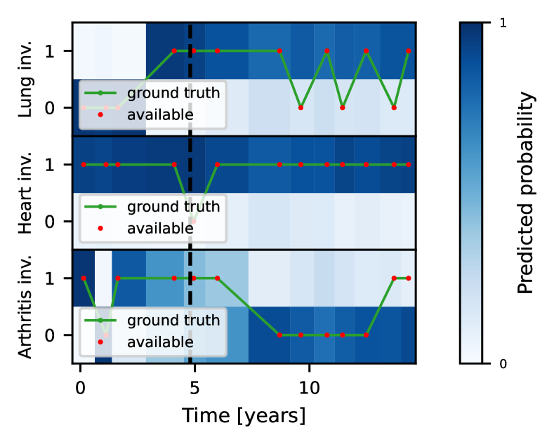
To illustrate how the model allows a holistic understanding of a patient’s disease course, we follow an index patient $p_{idx}$ throughout the experiments. This patient has a complex disease trajectory, with varying organ involvement and stages.

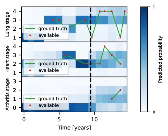
We can use our model to forecast the high-dimensional distribution of $\boldsymbol{x}_{1:T}$ and $\boldsymbol{y}_{1:T}$ given the past measurements $\boldsymbol{x}_{0:k}$, as described in subsection 3.7. For example, the heatmaps in LABEL:fig:inv_pat show the predicted probabilities of organ involvement at a given time, overlaid with the ground truth labels. The model forecasts the probabilities after the dashed line. We provide online prediction plots for additional $\boldsymbol{x}$ and $\boldsymbol{y}$ in Appendix D.1.1.

fig:inv_pat

Figure 4: Probabilities of organ involvement for $p_{idx}$.

4.2 Cohort Analysis

By learning the joint distribution $p(\boldsymbol{x},\boldsymbol{y},\boldsymbol{z})$, our model allows us to analyze cohort-level disease patterns through the analysis of $\boldsymbol{z}$. Furthermore, by learning $p(\boldsymbol{z}|\boldsymbol{c})$, we estimate the average prior disease trajectories in the cohort. We analyze these prior trajectories in Appendix D.2.1.

4.2.1 Latent Space and Medical Concepts

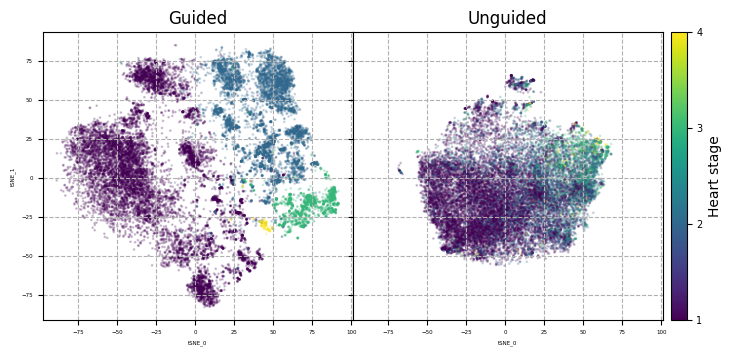
We aim to provide a method achieving semi-supervised disentanglement in the latent space. In LABEL:fig:guidance, we compare the distribution of medical concept ground truth labels (heart stage) in a guided versus an unguided model (i.e. without training any guidance networks). The guided model clearly provides higher medical concept disentanglement than the unguided model and thus enhances the interpretability of the different subspaces in $\boldsymbol{z}$.

fig:guidance

Figure 5: Guided versus unguided latent spaces.

In LABEL:fig:tsnes, we visualize the latent space overlaid with the different predicted probabilities of organ involvement. In red, we draw the latent space trajectory of $p_{idx}$, thus getting an understandable overview of its trajectory with respect to the different medical concepts. The solid line highlights the reconstructed trajectory, whereas the dotted lines are forecasted sampled trajectories.

fig:tsnes

Figure 6: Probabilities of lung and heart involvement in the latent space.

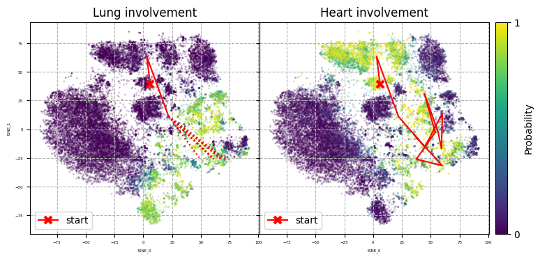
In the first panel of LABEL:fig:tsnes, we leverage the model’s generative abilities to sample forecasted $\boldsymbol{z}$ trajectories, providing estimates of future disease phases. The model forecasts that $p_{idx}$ will move towards a region with higher probabilities of lung and heart involvement. All of the sampled trajectories converge towards the same region in this case. The second panel is overlaid with the complete reconstructed trajectory of $p_{idx}$ in $\boldsymbol{z}$. The disentanglement in the latent space enables a straightforward overview of the past and future patient trajectory. Additionally, LABEL:fig:tsnes_stages in the appendix shows the patient trajectory overlaid with the predicted organ stages.

4.2.2 Clustering and Similarity of Patient Trajectories

As described in subsection 3.8, we compute the dynamic-time-warping similarity measure for the latent trajectories $\mathcal{H}_{i}=h(\mathcal{T}_{i})$, and subsequently apply k-means or k-nn to respectively cluster the multivariate time series $\{\mathcal{H}_{i}\}_{i=1}^{N}$ or find similar patient trajectories. We used the library implemented by Tavenard et al. (2020).

fig:clust_traj_all

Figure 7: Clustered trajectories in the latent space.

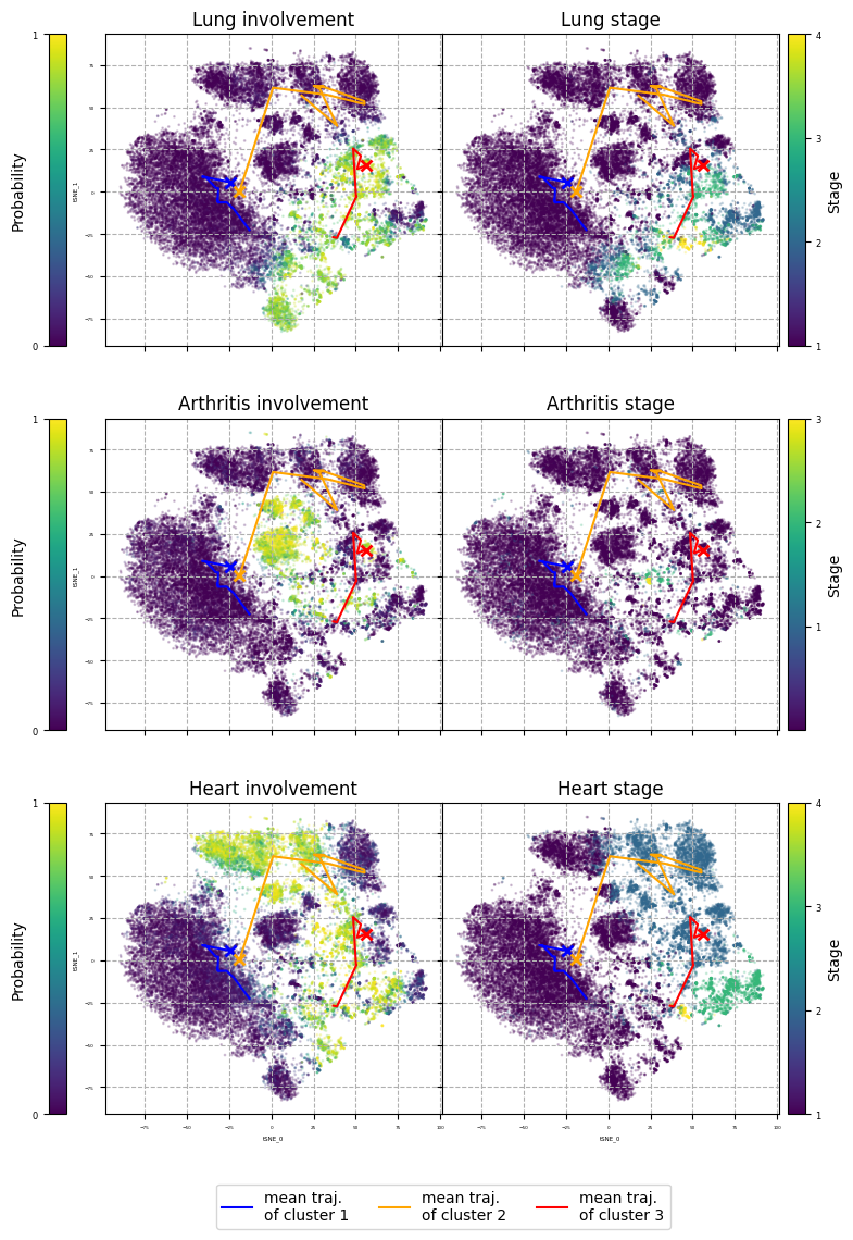
In LABEL:fig:clust_traj_all, we show the three mean cluster trajectories starting at the cross x in the latent space overlaid with the predicted medical concepts. The first found cluster corresponds to patients with no or little organ involvement. The second mean trajectory starts close to the first but progresses towards regions with heart involvement. The third cluster contains the most severely progressing patients. Furthermore, our modeling approach allows for direct computation of the medical concept probabilities for the mean cluster trajectories (LABEL:fig:clust_traj_proba in the appendix). Similarly, LABEL:fig:traj_p_simil and LABEL:fig:tsne_traj_p_simil in the appendix compare the medical concept and latent trajectories of $p_{idx}$ and its $3$ nearest neighbors.

5 Conclusion

In this study, we present a novel deep semi-supervised generative latent variable approach to model complex disease trajectories. By introducing the guidance networks, we propose a method to augment the unsupervised deep generative model with established medical concepts and achieve more interpretable and disentangled latent processes. Our non-discriminative approach effectively addresses important desiderata for healthcare models such as forecasting, uncertainty quantification, dimensionality reduction, and interpretability. Furthermore, we empirically show that our model is suited for a real-world use case, namely the modeling of systemic sclerosis, and enables a holistic understanding of the patients’ disease course. The disentangled latent space facilitates comprehensive trajectory visualizations and straightforward clustering, analysis, and forecasting of patient trajectories.

Both our presented experiments and modeling approaches hold the potential to be extended and adapted in many ways. We included here only the most pertinent experiments and opted for a simple architecture suited to SSc modeling. In future work, we intend to extend our framework to handle continuous time (Appendix B.2), include medications for generating future hypothetical conditional trajectories (Appendix B.3), include more organs in the modeling of SSc, and also include guidance networks to model additional disease dynamics like long-term outcomes. In particular, the clinical insights regarding the knowledge discovery gained from the clustering of trajectories such as finding new subtypes of SSc, identifying similar patients, and conducting a pathway analysis of the latent space, will be further explored in future work.

6 Data and Code Availability

The dataset used is owned by a third party, the EUSTAR group, and may be obtained by request after the approval and permission from EUSTAR. The code builds upon the pythae library (Chadebec et al., 2022). The code and examples using some artificial data are available at https://github.com/uzh-dqbm-cmi/eustar_dgm4h.

7 Acknowledgements

The authors thank the patients and caregivers who made the study possible, as well as all involved clinicians from the EUSTAR who collected the data. This work was funded by the Swiss National Science Foundation (project number 201184).

Appendix A Appendix

A.1 Clinical Insights for Systemic Sclerosis

In this paper, we present a general approach for modeling and analyzing complex disease trajectories, for which we used the progression of systemic sclerosis as an example. The focus of this paper is on the machine learning methodology, while clinically relevant insights and data analysis regarding systemic sclerosis will be discussed in a clinical follow-up paper where our model will be applied to investigate the involvement of multiple organs.

Since there is ongoing research and discussion towards finding optimal definitions of the medical concepts (involvement, stage, progression) for all impacted organs in SSc, we used preliminary definitions for three organs as a proof of concept.

A.2 Dataset

The European Scleroderma Trials and Research group (EUSTAR) maintains a registry dataset of about 20’000 patients extensively documenting organ involvement in SSc. It contains around $30$ demographic variables, and 500 temporal clinical measurement variables documenting the patients’ overall and organ-specific disease evolution. For a detailed description of the database, we refer the reader to Meier et al. (2012); Hoffmann-Vold et al. (2021).

For our analysis, we included $5673$ patients with enough temporality (i.e. at least $5$ medical visits). We used $10$ static variables related to the patients’ demographics and $34$ clinical measurement variables, mainly related to the monitoring of the lung, heart, and joints in SSc. In future work, we plan to include more patients and more clinical measurements for analyzing all involved organs.

A.3 Medical Concepts Definitions

Defining the organ involvement and stages in SSc is a challenging task as varying and sometimes contradicting definitions are used in different studies. However, there is ongoing research to find the most accurate definitions. Since this work is meant as a proof of concept, we used the following preliminary definitions of involvement and stage for the lung, heart, and joints (arthritis). The medical concepts are defined for the variables of the EUSTAR database. There are $4$ stages of increasing severity for each organ. If multiple definitions are satisfied, the most severe stage is selected. Furthermore, there is missingness in the labels due to incomplete clinical measurements. Our modeling approach thus also could be used to label the medical concepts when missing.

We use the following abbreviations:

• Interstitial Lung Disease: ILD

• High-resolution computed tomography: HRCT

• Forced Vital Capacity: FVC

• Left Ventricular Ejection Fraction: LVEF

• Brain Natriuretic Peptide: BNP

• N-terminal pro b-type natriuretic peptide: NTproBNP

• Disease Activity Score 28: DAS28

A.3.1 Lung

Involvement

At least one of the following must be present:

• ILD on HRCT

• FVC $<70\%$

Severity staging

1. FVC $>80\%$ or Dyspnea stage of $2$

2. ILD extent $<20\%$ or $70\%<\text{FVC}\leq 80\%$ or Dyspnea stage of $3$

3. ILD extent $>20\%$ or $50\%\leq\text{FVC}\leq 70\%$ or Dyspnea stage of $4$

4. FVC$<50\%$ or Lung transplant or Dyspnea stage of $4$

A.3.2 Heart

Involvement

At least one of the following must be present:

• LVEF $<45\%$

• Worsening of cardiopulmonary manifestations within the last month

• Abnormal diastolic function

• Ventricular arrhythmias

• Pericardial effusion on echocardiography

• Conduction blocks

• BNP $>35$ pg/mL

• NTproBNP$>125$ pg/mL

Severity staging

1. Dyspnea stage of $1$

2. Dyspnea stage of $2$

3. Dyspnea stage of $3$

4. Dyspnea stage of $4$

A.3.3 Arthritis

Involvement

At least one of the following must be present:

• Joint synovitis

• Tendon friction rubs

Severity staging

1. DAS28 $<2.7$

2. $2.7\leq\text{DAS28}\leq 3.2$

3. $3.2<\text{DAS28}\leq 5.1$

4. DAS28 $>5.1$

Appendix B Details and Extensions for Generative Model

In this section, we provide more details and several possible extensions to the main temporal generative model presented in Section 3.1.

B.1 Inference

In this section, we explain the inference process of the proposed generative model $p_{\psi}(\boldsymbol{y},\boldsymbol{x},\boldsymbol{z}|\boldsymbol{c})=p_{\gamma}(\boldsymbol{y}|\boldsymbol{z},\boldsymbol{c})p_{\pi}(\boldsymbol{x}|\boldsymbol{z},\boldsymbol{c})p_{\phi}(\boldsymbol{z}|\boldsymbol{c})$ in more detail. We are particularly interested in the posterior of the latent variables $\boldsymbol{z}$ given $\boldsymbol{y}$, $\boldsymbol{x}$, and $\boldsymbol{c}$, that is,

$$p_{\psi}(\boldsymbol{z}|\boldsymbol{y},\boldsymbol{x},\boldsymbol{c})=\frac{p_{\psi}(\boldsymbol{y},\boldsymbol{x},\boldsymbol{z}|\boldsymbol{c})}{p_{\psi}(\boldsymbol{y},\boldsymbol{x}|\boldsymbol{c})}=\frac{p_{\psi}(\boldsymbol{y},\boldsymbol{x},\boldsymbol{z}|\boldsymbol{c})}{\int p_{\psi}(\boldsymbol{y},\boldsymbol{x},\boldsymbol{z}|\boldsymbol{c})d\boldsymbol{z}},$$

which is in general intractable due to the marginalization of the latent process in the marginal likelihood $p_{\psi}(\boldsymbol{y},\boldsymbol{x}|\boldsymbol{c})=\int p_{\psi}(\boldsymbol{y},\boldsymbol{x},\boldsymbol{z}|\boldsymbol{c})d\boldsymbol{z}$. Therefore, we resort to approximate inference, in particular, amortized variational inference (VI) (Blei et al., 2017), where a variational distribution $q_{\theta}(\boldsymbol{z}|\boldsymbol{x},\boldsymbol{c})$ close to the true posterior distribution $p_{\psi}(\boldsymbol{z}|\boldsymbol{x},\boldsymbol{y},\boldsymbol{c})\approx q_{\theta}(\boldsymbol{z}|\boldsymbol{x},\boldsymbol{c})$ is introduced. The similarity between these distributions is usually measured in terms of KL divergence (Murphy, 2022), therefore, we aim to find parameters satisfying

$$\theta^{*},\psi^{*}=\operatorname*{argmin}_{\theta,\psi}KL\left[q_{\theta}(\boldsymbol{z}|\boldsymbol{x},\boldsymbol{c})~{}||~{}p_{\psi}(\boldsymbol{z}|\boldsymbol{x},\boldsymbol{y},\boldsymbol{c})\right].$$

This optimization problem is equivalent (Murphy, 2022) to maximizing a lower bound $\mathcal{L}(\psi,\theta;\boldsymbol{x},\boldsymbol{y},\boldsymbol{c})\leq p_{\psi}(\boldsymbol{y},\boldsymbol{x}|\boldsymbol{c})$ to the intractable marginal likelihood, that is,

$$\theta^{*},\psi^{*}=\operatorname*{argmax}_{\theta,\psi}\mathcal{L}(\psi,\theta;\boldsymbol{x},\boldsymbol{y},\boldsymbol{c}).$$

In particular, this lower bound equals

$$\mathcal{L}= \int q_{\theta}(\boldsymbol{z}|\boldsymbol{x},\boldsymbol{c})\log\frac{p_{\psi}(\boldsymbol{y},\boldsymbol{x},\boldsymbol{z}|\boldsymbol{c})}{q_{\theta}(\boldsymbol{z}|\boldsymbol{x},\boldsymbol{c})}d\boldsymbol{z}$$

$$= \int q_{\theta}(\boldsymbol{z}|\boldsymbol{x},\boldsymbol{c})\log\frac{p_{\gamma}(\boldsymbol{y}|\boldsymbol{z},\boldsymbol{c})p_{\pi}(\boldsymbol{x}|\boldsymbol{z},\boldsymbol{c})p_{\phi}(\boldsymbol{z}|\boldsymbol{c})}{q_{\theta}(\boldsymbol{z}|\boldsymbol{x},\boldsymbol{c})}d\boldsymbol{z},$$

which can be rearranged to

$$\mathcal{L}= ~{}\mathbb{E}_{q_{\theta}(\boldsymbol{z}|\boldsymbol{x},\boldsymbol{c})}\left[\log p_{\pi}(\boldsymbol{x}|\boldsymbol{z},\boldsymbol{c})\right]$$

$$+ ~{}\mathbb{E}_{q_{\theta}(\boldsymbol{z}|\boldsymbol{x},\boldsymbol{c})}\left[\log p_{\gamma}(\boldsymbol{y}|\boldsymbol{z},\boldsymbol{c})\right]$$

$$- ~{}KL\left[q_{\theta}(\boldsymbol{z}|\boldsymbol{x},\boldsymbol{c})~{}||~{}p_{\phi}(\boldsymbol{z}|\boldsymbol{c})\right].$$

For the Gaussian prior and approximate posterior described in Section 3.2 and 3.5, respectively, the KL-term can be computed analytically and efficiently (Tomczak, 2022). On the other hand, the expectations $\mathbb{E}_{q_{\theta}}$ can be approximated with a few Monte-Carlo samples $\boldsymbol{z}^{1},\ldots,\boldsymbol{z}^{s},\ldots,\boldsymbol{z}^{S}\sim q_{\theta}(\boldsymbol{z}|\boldsymbol{x},\boldsymbol{c})$ leading to

$$\mathbb{E}_{q_{\theta}(\boldsymbol{z}|\boldsymbol{x},\boldsymbol{c})}\left[\log p_{\pi}(\boldsymbol{x}|\boldsymbol{z},\boldsymbol{c})p_{\gamma}(\boldsymbol{y}|\boldsymbol{z},\boldsymbol{c})\right]$$

$$\approx\frac{1}{S}\sum_{s=1}^{S}\log p_{\pi}(\boldsymbol{x}|\boldsymbol{z}^{s},\boldsymbol{c})p_{\gamma}(\boldsymbol{y}|\boldsymbol{z}^{s},\boldsymbol{c}).$$

B.1.1 Partially Observed Data

The measurements $\boldsymbol{x}\in\mathbb{R}^{D\times T}$ and the concepts $\boldsymbol{y}\in\mathbb{R}^{P\times T}$ contain many missing values. We define the indices $\boldsymbol{o}_{x}\in\mathbb{R}^{D\times T}$ and $\boldsymbol{o}_{y}\in\mathbb{R}^{P\times T}$ for which the observations are actually measured. Therefore, we compute the lower bound only on the observed variables, i.e. $\log p_{\psi}(\boldsymbol{x}^{\boldsymbol{o}_{x}},\boldsymbol{y}^{\boldsymbol{o}_{y}}|\boldsymbol{c})\geq\mathcal{L}(\psi,\theta;\boldsymbol{x}^{\boldsymbol{o}_{x}},\boldsymbol{y}^{\boldsymbol{o}_{y}},\boldsymbol{c})$, as is similarly done by Fortuin et al. (2020); Ramchandran et al. (2021). This then leads for instance to

$$\mathbb{E}_{q_{\theta}(\boldsymbol{z}|\boldsymbol{x},\boldsymbol{c})}\left[\log p_{\pi}(\boldsymbol{x}^{\boldsymbol{o}_{x}}|\boldsymbol{z},\boldsymbol{c})p_{\gamma}(\boldsymbol{y}^{\boldsymbol{o}_{y}}|\boldsymbol{z},\boldsymbol{c})\right],$$

where the related log-likelihood $\log p_{\pi}(\boldsymbol{x}^{\boldsymbol{o}_{x}}|\boldsymbol{z},\boldsymbol{c})=\log\prod_{t,d\in\boldsymbol{o}_{x}}p_{\pi}(x_{t}^{d}|\boldsymbol{z}_{t},\boldsymbol{c}_{t})=\sum_{t,d\in\boldsymbol{o}_{x}}\log p_{\pi}(x_{t}^{d}|\boldsymbol{z}_{t},\boldsymbol{c}_{t})$ is only summed over the actually observed measurements. The same can be derived for the medical concepts $\boldsymbol{y}^{\boldsymbol{o}_{y}}$.

B.1.2 Lower Bound for N Samples

Given a dataset with $N$ $\mathrm{iid}$ patients $\mathcal{D}=\{\mathcal{D}_{i}\}_{i=1}^{N}=\{\boldsymbol{x}_{1:T_{i}}^{i},\boldsymbol{y}_{1:T_{i}}^{i},\boldsymbol{c}_{1:T_{i}}^{i}\}_{i=1}^{N}$, the lower bound to the marginal log-likelihood is

$$\log p_{\psi}(\mathcal{D})=\log\prod_{i=1}^{N}p_{\psi}(\mathcal{D}_{i})\geq\sum_{i=1}^{N}\mathcal{L}(\psi,\theta;\boldsymbol{x}^{i},\boldsymbol{y}^{i},\boldsymbol{c}^{i}),$$

which is maximized through stochastic optimization with mini-batches (subsection 3.6). Moreover, suppose we have $T+1$ iid copies of the whole dataset $\{\mathcal{D}^{k}\}_{k=0}^{T}$, then

$$\log p_{\psi}(\{\mathcal{D}^{k}\}_{k=0}^{T})=\log\prod_{i=1}^{N}\prod_{k=0}^{T}p_{\psi}(\mathcal{D}_{i}^{k})$$

$$\geq\sum_{i=1}^{N}\sum_{k=0}^{T}\mathcal{L}_{k}(\psi,\theta;\boldsymbol{x}^{i,k},\boldsymbol{y}^{i,k},\boldsymbol{c}^{i,k}),$$

where $\mathcal{L}_{k}(\psi,\theta;\boldsymbol{x}^{i,k},\boldsymbol{y}^{i,k},\boldsymbol{c}^{i,k})$ is the lower bound obtained by plugging in the corresponding approximate posterior $q_{\theta}(\boldsymbol{z}|\boldsymbol{x}_{0:k},\boldsymbol{c})$.

B.1.3 Predictive Distributions

The predictive distributions for the measurement $\boldsymbol{x}_{1:T}$ and concept trajectories $\boldsymbol{y}_{1:T}$ in subsection 3.7 can be obtained via a two-stage Monte-Carlo approach. For instance, we can sample from the distribution of the measurements

$$q_{*}(\boldsymbol{x}_{1:T}|\boldsymbol{x}_{0:k},\boldsymbol{c})$$

$$= \int p_{\pi^{*}}(\boldsymbol{x}_{1:T}|\boldsymbol{z}_{1:T},\boldsymbol{c})q_{\theta^{*}}(\boldsymbol{z}_{1:T}|\boldsymbol{x}_{0:k},\boldsymbol{c})d\boldsymbol{z}$$

by first sampling from the latent trajectories

$$\boldsymbol{z}_{1:T}^{1},\ldots,\boldsymbol{z}_{1:T}^{s},\ldots\boldsymbol{z}_{1:T}^{S}\sim q_{\theta^{*}}(\boldsymbol{z}_{1:T}|\boldsymbol{x}_{0:k},\boldsymbol{c})$$

given the current observed measurements $\boldsymbol{x}_{1:k}$. In a second step, for each of the samples, we compute

$$\boldsymbol{x}_{1:T}^{1},\ldots,\boldsymbol{x}_{1:T}^{u},\ldots\boldsymbol{x}_{1:T}^{U}\sim p_{\pi^{*}}(\boldsymbol{x}_{1:T}|\boldsymbol{z}_{1:T}^{s},\boldsymbol{c})$$

to represent the overall uncertainty of the measurement distribution.

B.2 Different Prior

The factorized prior described in subsection 3.2 can be extended to continuous time with Gaussian processes (GPs, Williams and Rasmussen (2006); Schürch et al. (2020, 2023a)), as introduced by Casale et al. (2018); Fortuin et al. (2020) in the unsupervised setting. In particular, we can replace

$$p_{\phi}(\boldsymbol{z}|\boldsymbol{c}) =p_{\phi}(\boldsymbol{z}_{1:T}|\boldsymbol{c}_{1:T})=\prod_{t=1}^{T}\prod_{l=1}^{L}p_{\phi}(\boldsymbol{z}_{t}^{l}|\boldsymbol{c}_{t})$$

$$=\prod_{t=1}^{T}\prod_{l=1}^{L}\mathcal{N}\left(\boldsymbol{z}_{t}^{l}|\mu_{\phi}^{l}(\boldsymbol{c}_{t}),\sigma^{l}_{\phi}(\boldsymbol{c}_{t})\right),$$

with

$$p_{\phi}(\boldsymbol{z}_{1:T}|\boldsymbol{c}_{1:T})=\prod_{l=1}^{L}\mathcal{GP}\left(\boldsymbol{z}^{l}|m_{\phi}^{l}(\boldsymbol{c}),k^{l}_{\phi}(\boldsymbol{c},\boldsymbol{c}^{\prime})\right)$$

with a mean function $m_{\phi}^{l}(\boldsymbol{c})$ and kernel $k^{l}_{\phi}(\boldsymbol{c},\boldsymbol{c}^{\prime})$, to take into account all the probabilistic correlations occurring in continuous time. This leads to a stochastic dynamic process, which theoretically matches the assumed disease process more adequately than a deterministic one. A further advantage is the incorporation of prior knowledge via the choice of the particular kernels for each latent process so that different characteristics such as long and small lengthscales, trends, or periodicity can be explicitly enforced in the latent space.

B.3 Conditional Generative Trajectory Generation

Our generative approach is also promising for conditional generative trajectory sampling, in a similar spirit as proposed by Schürch et al. (2023b). In particular, if we use medications as additional covariates $\boldsymbol{p}=\boldsymbol{p}_{1:T}=\{\boldsymbol{p}_{0:k},\boldsymbol{p}_{k+1:T}\}$ in our approximate posterior distribution $q_{\theta}(\boldsymbol{z}|\boldsymbol{x}_{0:k},\boldsymbol{c})=q_{\theta}(\boldsymbol{z}|\boldsymbol{x},\boldsymbol{\tau},\boldsymbol{s},\boldsymbol{p}_{0:k},\boldsymbol{p}_{k+1:T})$ with $\boldsymbol{c}=\{\boldsymbol{\tau},\boldsymbol{s},\boldsymbol{p}\}$, the model can be used to sample future hypothetical trajectories $\boldsymbol{x}_{k+1:T}$ with

$$q_{*}(\boldsymbol{x}_{k+1:T}|\boldsymbol{x}_{0:k},\boldsymbol{\tau},\boldsymbol{s},\boldsymbol{p}_{0:k},\boldsymbol{p}_{k+1:T})$$

$$=\int p_{\pi^{*}}(\boldsymbol{x}_{k+1:T}|\boldsymbol{z},\boldsymbol{\tau},\boldsymbol{s},\boldsymbol{p}_{0:k},\boldsymbol{p}_{k+1:T})$$

$$q_{\theta^{*}}(\boldsymbol{z}|\boldsymbol{x}_{0:k},\boldsymbol{\tau},\boldsymbol{s},\boldsymbol{p}_{0:k},\boldsymbol{p}_{k+1:T})d\boldsymbol{z}$$

based on future query medications $\boldsymbol{p}_{k+1:T}$.

Appendix C Model Implementation

C.1 Model Architecture

We describe the architecture and inputs/outputs of the different neural networks in our final model for SSc. For a patient with measurement time points $\boldsymbol{\tau}_{1:T}$ of the complete trajectory, the model input at time $t\in\boldsymbol{\tau}$ are the static variables $\boldsymbol{s}$, the clinical measurements $\boldsymbol{x}_{0:t}$, and the trajectory time points $\boldsymbol{\tau}$. Thus for SSc modeling, we have that $\boldsymbol{c}=\{\boldsymbol{\tau},\boldsymbol{s}\}$. The model $\mathcal{M}$ outputs the distribution parameters of the clinical measurements and the organ labels for all trajectory time points $\boldsymbol{\tau}$. Without loss of generality, we assume that $\boldsymbol{x}^{1:M}$ are continuous variables and $\boldsymbol{x}^{M+1:D}$ categorical, so that the model can be described as

$$\mathcal{M}:\left(\boldsymbol{c},\boldsymbol{x}_{0:t}\right)\longrightarrow$$

$$\left(\hat{\boldsymbol{\mu}}_{1:T}^{x^{1:M}}(t),\hat{\boldsymbol{\sigma}}_{1:T}^{x^{1:M}}(t),\hat{\boldsymbol{\pi}}_{1:T}^{x^{M+1:D}}(t),\hat{\boldsymbol{\pi}}_{1:T}^{y}(t)\right).$$

We explicitly include the dependencies to $t$ to emphasize that the parameters of the whole trajectory are estimated given the information up to time $t$.

• Prior network: The prior is a multilayer perceptron (MLP). It takes as input $\boldsymbol{c}$ and outputs the estimated mean and variance of the prior latent distribution $\hat{\mu}_{1:T}^{prior}$ and $\hat{\sigma}_{1:T}^{prior}$.

• Encoder network (posterior): The encoder contains LSTM layers followed by fully connected feed-forward layers. It takes as input $\boldsymbol{x}_{0:t}$ and $\boldsymbol{c}$ and outputs the estimated mean and standard deviation of the posterior distribution of the latent variables $\hat{\mu}_{1:T}^{post}(t)$ and $\hat{\sigma}_{1:T}^{post}(t)$, from which we sample the latent variables $\boldsymbol{z}_{1:T}(t)$ (complete temporal latent process) given the information up to $t$.

• Decoder network (likelihood): The decoder is an MLP and takes as input the sampled latent variables $\boldsymbol{z}_{1:T}(t)$ and $\boldsymbol{c}$ and outputs the estimated means and standard deviations $\hat{\mu}_{1:T}^{x^{1:M}}(t)$ and $\hat{\sigma}_{1:T}^{x^{1:M}}(t)$ of the distribution of the continuous clinical measurements and class probabilities $\hat{\pi}_{1:T}^{x^{M+1:D}}(t)$ of the categorical measurements.

• Guidance networks: For each organ, we define one MLP guidance network per related medical concept (involvement and stage). A guidance network for organ $o\in\mathcal{O}:=\{lung,heart,joints\}$ and related medical concept $m\in\{inv,stage\}$, takes as input the sampled latent variables $\boldsymbol{z}_{1:T}^{\epsilon(o(m))}(t)$ and outputs the predicted class probabilities $\hat{\pi}_{1:T}^{y^{\nu(o(m))}}(t)$ of the labels, where $\nu(o(m))$ are the indices in $y$ related to the medical concept $o(m)$, and $\epsilon(o(m))$ the indices in the latent space.

C.2 Training Objective

We follow the notation introduced in Section 3 and Appendix B. To train the model to perform forecasting, for each patient, we augment the data by assuming $T+1$ iid copies of the data $x$ and $y$ (see also B.1.2) and recursively try to predict the last $T-t$, $t=0,...,T$ clinical measurements and medical concepts. The total loss for a patient $p$ is

$$\mathcal{L}_{p}=\sum_{t=0}^{T}\mathcal{L}(t),$$ (1)

where

$$\mathcal{L}(t):=NLL\left(\hat{\mu}^{x^{1:M}}(t),\hat{\sigma}^{x^{1:M}}(t),\boldsymbol{x}^{1:M}\right)$$

$$+CE\left(\hat{\pi}^{x^{M+1:D}}(t),\boldsymbol{x}^{M+1:D}\right)$$

$$+\alpha*CE\left(\hat{\pi}^{y}(t),\boldsymbol{y}\right)$$

$$+\beta*KL\left(\hat{\mu}^{prior},\hat{\sigma}^{prior},\hat{\mu}^{post}(t),\hat{\sigma}^{post}(t)\right),$$

where $NLL$, $CE$ and $KL$ are the negative log-likelihood, cross-entropy and KL divergence, respectively. Further, $\alpha$ and $\beta$ are hyperparameters weighting the guidance and KL terms.

C.2.1 Model Optimization

We only computed the loss with respect to the available measurements. We randomly split the set of patients $\mathcal{P}$ into a train set $\mathcal{P}_{train}$ and test set $\mathcal{P}_{test}$ and performed $5-$fold CV with random search on $\mathcal{P}_{train}$ for hyperparameter tuning. Following the principle of empirical risk minimization, we trained our model to minimize the objective loss over $\mathcal{P}_{train}$, using the Adam (Kingma and Ba, 2014) optimizer with mini-batch processing and early stopping.

C.2.2 Architecture and Hyperparameters

We tuned the dropout rate and the number and size of hidden layers using $5$-fold CV, and used a simple architecture for our final model. The posterior network contains a single lstm layer with hidden state of size $100$, followed by two fully connected layers of size $100$. The likelihood network contains two separate fully connected layers of size $100$, learning the mean and variances of the distributions separately. The guidance networks contain a single fully connected layer of size $40$ and the prior network a single fully connected layer of size $50$. We used batch normalization, ReLU activations, and a dropout rate of $0.1$. We set $\alpha=0.2$ and $\beta=0.01$.

Appendix D Results

D.1 Model Evaluation

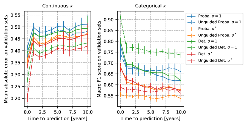
We discuss the evaluation results for unguided models, medical concept prediction, and uncertainty quantification. In LABEL:fig:perf_x_bsl, we compare the performance of the clinical measurement $\boldsymbol{x}$ prediction of the different guided models versus their unguided counterparts (with the same number of latent processes). Note that these unguided models are optimal baselines for $\boldsymbol{x}$ prediction since they are not trained to predict $\boldsymbol{y}$, too. As LABEL:fig:perf_x_bsl shows, the unguided models usually outperform the guided models, but the difference is not significant for the probabilistic models. Unsurprisingly, the best performing model is a deterministic unguided model, i.e. not trained to learn the $\boldsymbol{z}$ and $\boldsymbol{y}$ distributions.

fig:perf_x_bsl

Figure 8: Performance for $x$ prediction, guided versus unguided models.

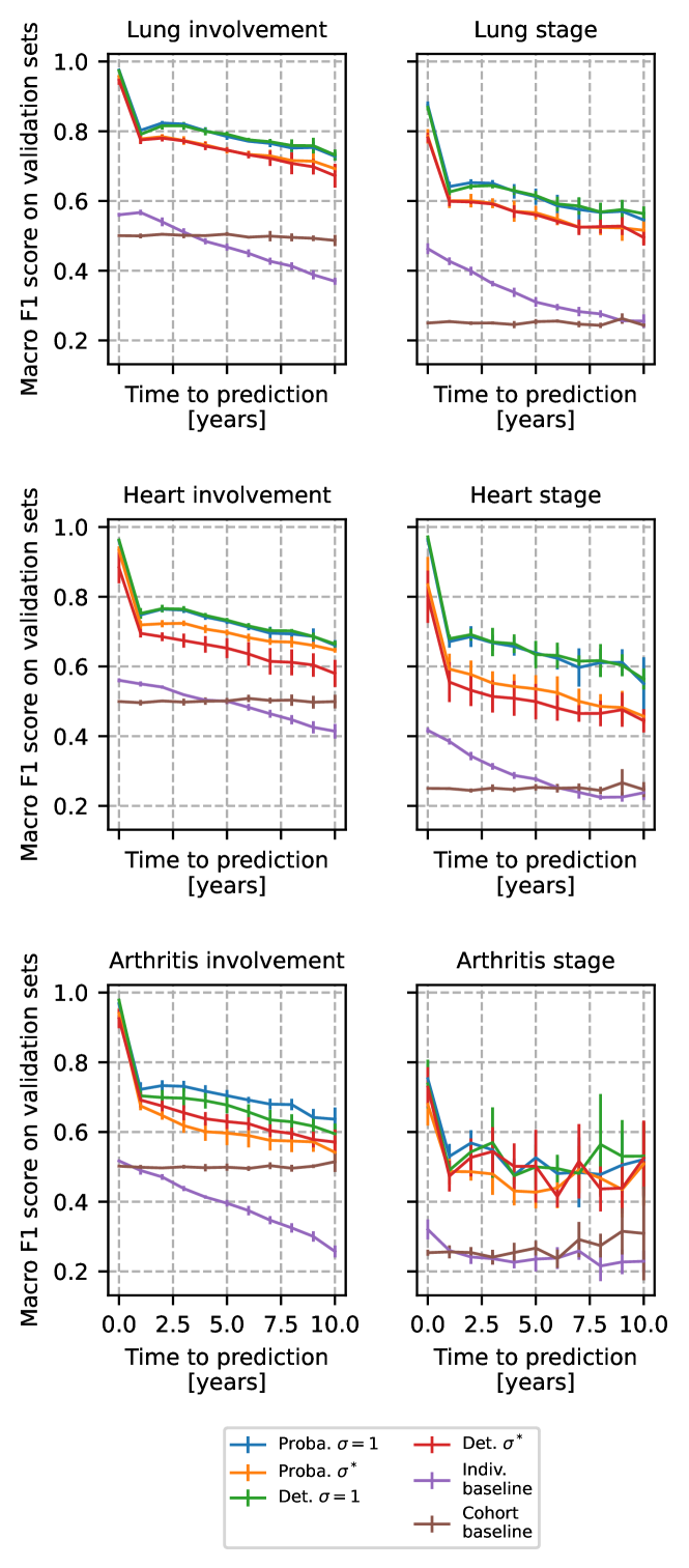
LABEL:fig:perf_y shows the macro $F_{1}$ scores for the medical concepts $\boldsymbol{y}$ prediction of the different models. The models with fixed likelihood variance generally slightly outperform the models with learned variance. All of the models outperform the individualized and cohort baselines.

fig:perf_y

Figure 9: Performance for $y$ prediction.

To evaluate the uncertainty quantification of the models, we computed the coverage of the continuous predictions and calibration of the predicted probabilities for categorical measurements. The coverage is the probability that the confidence interval (CI) predicted by the model contains the true data point. Since the likelihood distribution is Gaussian, the 95% CI is $\mu_{pred}\pm 1.96\sigma_{pred}$. To achieve perfect coverage of the $95\%$ CI, the predictions should fall within the predicted CI $95\%$ of the time. We computed the coverage over all forecasted data points. For categorical measurements, the calibration curve is computed to assess the reliability of the predicted class probabilities. They are computed in the following way. We grouped all of the forecasted probabilities (for one-hot encoded vectors) into $n=20$ bins dividing the 0-1 interval. Then, for each bin, we compared the observed frequency of ground truth positives (aka “fraction of positive”) with the average predicted probability within the bin. Ideally, these two quantities should be as close as possible, i.e. close to the line of “perfect calibration” in LABEL:fig:calib. The calibration curves in LABEL:fig:calib show that all of the models are well calibrated both in their categorical $\boldsymbol{x}$ and medical concept $\boldsymbol{y}$ forecasts (averaged over all forecasted data points in the respective validation sets).

fig:calib [Categorical clinical measurements $x$][c]

Figure 10: Calibration curves.

[Medical concepts $y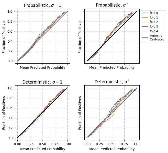$][c]

D.1.1 Online Prediction with Uncertainty

We provide additional online prediction results for the index patient $p_{idx}$.

Figures LABEL:fig:fvc and LABEL:fig:dlco_pat show the evolution in the predicted mean and $95\%$ CI of the Forced Vital Capacity (FVC) and DLCO(SB) for $p_{idx}$.

The values after the dashed line are forecasted. As more prior information becomes available to the model, the forecast becomes more accurate and the CI shrinks.

fig:fvc

Figure 11: FVC of $p_{idx}$: predicted mean and $95\%$ CI

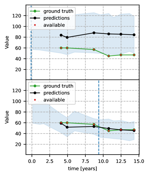
fig:dlco_pat

Figure 12: DLCO(SB) of $p_{idx}$: predicted mean and $95\%$ CI

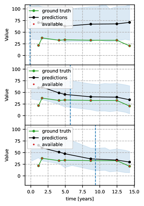
Figure LABEL:fig:stage_pat shows predicted probabilities of organ stages at a given time point. The intensity of the heatmap reflects the predicted probability.

fig:stage_pat

Figure 13: Probabilities of organ stages for $p_{idx}$.

D.2 Cohort Analysis

We present here additional cohort-level experiments using our model.

D.2.1 Prior z Distributions

fig:prior_pred

Figure 14: Prior predicted $\boldsymbol{x}$ trajectories conditioned on time and static variables.

[Prior FVC trajectories overlaid with different SSC subsets.]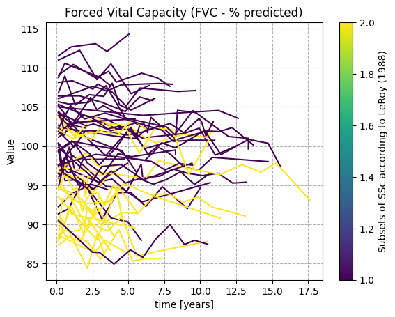

[Prior natriuretic peptides trajectories overlaid with date of birth.]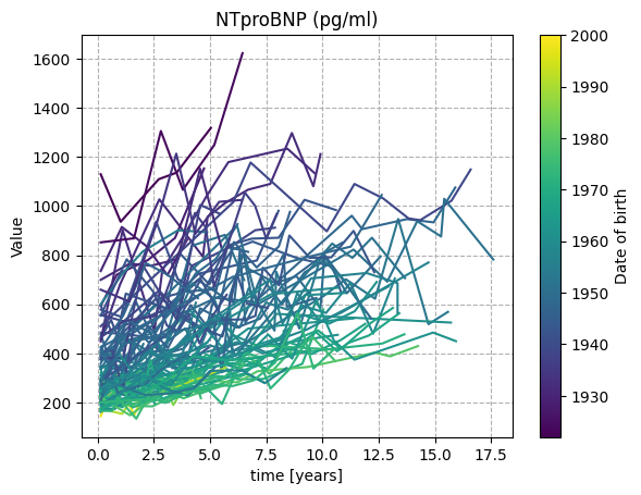

By learning $p(\boldsymbol{x},\boldsymbol{y}|\boldsymbol{s},\boldsymbol{\tau})$, we estimate the average prior disease trajectories in the cohort. This allows the comparison of trajectories, conditioned only on the simple subset of variables $\boldsymbol{s}$ and $\boldsymbol{\tau}$ and thus without facing any confounding in the trajectories, for instance, due to past clinical measurements $\boldsymbol{x}$. For example, in Figure Figure 14 we overlaid the predicted prior trajectories of Forced Vital Capacity (FVC) for a subset of patients in $\mathcal{P}_{test}$ with a static variable corresponding to the SSc subtype. Overall, the FVC values are predicted to remain quite stable over time, but with different average values depending on the SSc subtype. In Figure Figure 14, the prior predicted N-terminal pro b-type natriuretic peptide (NTproBNP) trajectories overlaid with age, show that the model predicts an overall increase in NTproBNP over time, and steeper for older patients.

D.2.2 Latent Space and Medical Concepts

fig:tsnes_stages

Figure 15: Predicted organ stages in the latent space. The red line highlights the trajectory of $p_{idx}$.

$\bf{t-}$SNEs:

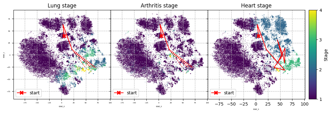
The $t$-SNE (Van der Maaten and Hinton, 2008) graphs were obtained by computing the two-dimensional $t$-SNE projection of the latent variables $\boldsymbol{z}_{1:T}\mid(\boldsymbol{x}_{1:T},\boldsymbol{c})$ (i.e. only using reconstructed $\boldsymbol{z}$) of a subset of $\mathcal{P}_{train}$ and then transforming and plotting the projected latent variables (reconstructed or forecasted) from patients in $\mathcal{P}_{test}$ (Poličar et al., 2019).

In LABEL:fig:tsnes, we showed the trajectory of $p_{idx}$ overlaid with the predicted organ involvement probabilities. In LABEL:fig:tsnes_stages, we additionally show the trajectory overlaid with the organ stages, showing for instance in the first panel that the model predicts an increase in the lung stage and in the last panel that $p_{idx}$ undergoes many different heart stages throughout the disease course.

D.2.3 Clustering of Patient Trajectories and Trajectory Similarity

We discuss additional results obtained through clustering and similarity analysis of latent trajectories (subsubsection 4.2.2). In LABEL:fig:clust_traj_proba, we show the different predicted probabilities of the medical concepts $\boldsymbol{y}$ for the mean trajectories within the three found clusters. This reveals which medical concepts are most differentiated by the clustering algorithm. For instance, cluster one exhibits low probabilities of organ involvement, while cluster two shows increasing probabilities of heart involvement and low probabilities of lung involvement. In contrast, cluster three shows increasing probabilities for both heart and lung involvement.

fig:tsne_traj_p_simil

Figure 16: Trajectory of $p_{idx}$ and its $3$ nearest neighbors in the latent space.

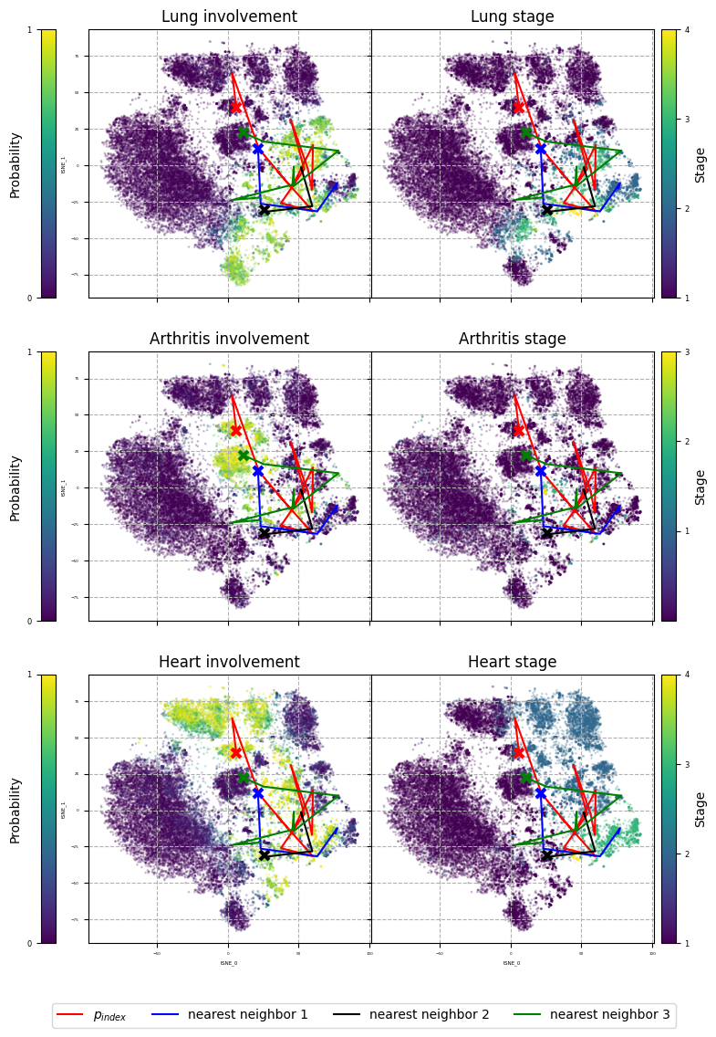
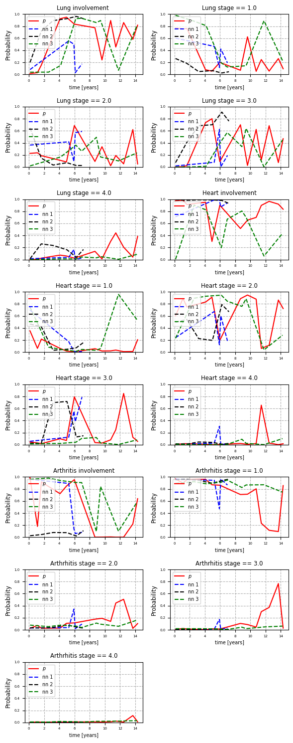
Additionally, we apply a k-nn algorithm with the dtw distance in the latent space to find patients with similar trajectories to $p_{idx}$. LABEL:fig:tsne_traj_p_simil shows the trajectory of $p_{idx}$ and its three nearest neighbors in the latent space. We can see that the nearest neighbors also have an evolving disease, going through various organ involvements and stages. Similarly, in LABEL:fig:traj_p_simil, the medical concept trajectories of $p_{idx}$ and its nearest neighbors reveal consistent patterns.

fig:clust_traj_proba

Figure 17: Medical concept trajectories for cluster means.

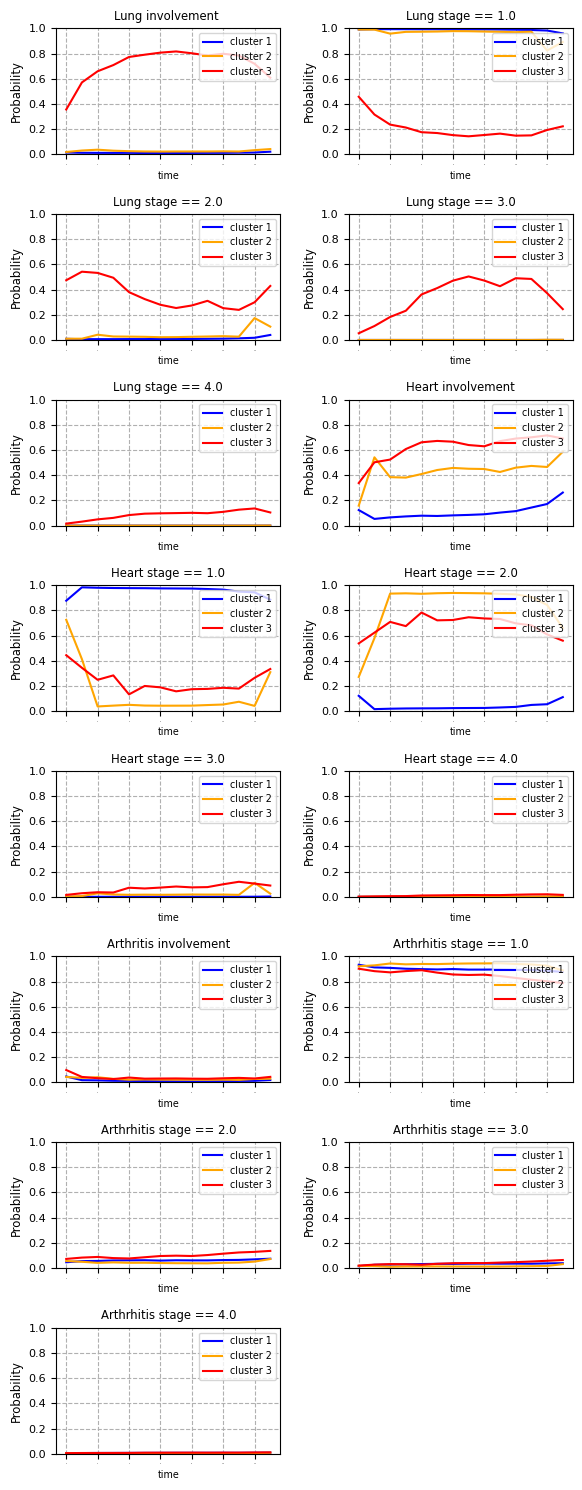
fig:traj_p_simil

Figure 18: Medical concept trajectories for $p_{idx}$ and its $3$ nearest neighbors.

Appendix E Deep Generative Temporal Models

In this section, we provide an extended background about different aspects of deep generative temporal models.

E.1 Probabilistic Generative Models

Probabilistic generative models differ from deterministic discriminative models in two key aspects. First, probabilistic models provide richer information by learning not only the mean $\mathbb{E}_{p(\boldsymbol{y})}[\boldsymbol{y}]$ but also the complete distribution $p(\boldsymbol{y})$, which can be used for instance for uncertainty quantification. Second, generative models learn the entire distribution $p(\boldsymbol{y},\boldsymbol{x})=p(\boldsymbol{y}|\boldsymbol{x})p(\boldsymbol{x})$, capturing the joint distribution over all involved variables $\boldsymbol{y}$ and $\boldsymbol{x}$. In contrast, discriminative models only learn the conditional distribution $p(\boldsymbol{y}|\boldsymbol{x})$ by separating target and output variables, without gaining knowledge about $\boldsymbol{x}$. Generative models allow to generate new samples from the learned distribution, offering a more holistic approach to modeling data. There are several other deep generative approaches besides latent variable models, for which we refer to Tomczak (2022).

E.2 Conditional Generative Models

Generative models can be enhanced by incorporating additional context variables $\boldsymbol{c}$, leading to the conditional generative model $p(\boldsymbol{y},\boldsymbol{x}|\boldsymbol{c})=p(\boldsymbol{y}|\boldsymbol{x},\boldsymbol{c})p(\boldsymbol{x}|\boldsymbol{c}),$ which could for instance model the interplay between the variables $\boldsymbol{y}$ and $\boldsymbol{x}$ given the personalized context $\boldsymbol{c}$. This distribution can be useful to generate novel realistic samples of $\boldsymbol{y}$-$\boldsymbol{x}$ pairs, conditioned on the individual past context or a specific condition.

E.3 Latent Variable Models

Probabilistic generative models can be extended by some latent variables $\boldsymbol{z}$, which reflects the assumption that not all variables are observed. This allows to model a generative process involving the observed variables $\boldsymbol{y}$ and $\boldsymbol{x}$, as well as some latent variables $\boldsymbol{z}$ by modeling the joint distribution $p(\boldsymbol{y},\boldsymbol{x},\boldsymbol{z})$, where the latent variables are learned during inference and marginalized out for prediction or other queries. These probabilistic representations can be used for identifying new patterns or concepts, not explicitly present in the data. Furthermore, they also allow modeling much more complex distributions beyond standard parametric distributions.

E.4 Temporal Generative Models

In the context of generative models, the variables can be represented as vectors or matrices, with the option to explicitly index them by time, denoted as $\boldsymbol{x}_{t}$. This temporal indexing enables the modeling of dynamical systems or time series $\boldsymbol{x}_{1:T}=[\boldsymbol{x}_{1},\ldots,\boldsymbol{x}_{t},\ldots,\boldsymbol{x}_{T}]$. Various approaches exist for modeling temporal data, such as discrete-time and continuous-time models, as well as deterministic and stochastic dynamic process models. The key distinction lies in how the variables relate to each other over time. For discrete-time models, the variables are updated at specific time intervals, making them suitable for systems that evolve in distinct steps. On the other hand, continuous-time models allow for a more seamless representation of systems that change continuously over time or are irregularly measured, providing a more accurate description of certain processes. Deterministic dynamic process models assume that the relationship between all time steps is completely predictable and certain. For instance, given the initial $\boldsymbol{x}_{1}$ state, all future steps are completely determined by a deterministic process. In contrast, probabilistic dynamic process models introduce an element of uncertainty, thus assuming that the evolution of the system from $\boldsymbol{x}_{t-1}$ to $\boldsymbol{x}_{t}$ is subject to probabilistic influences.

E.5 Deep Probabilistic Generative Models

Deep generative models constitute a very powerful class of probabilistic generative models, where deep neural networks (powerful function approximators) are used to parameterize distributions. Consider a parametric conditional distribution $p(\boldsymbol{y}|\boldsymbol{x})$ with parameters $\mu_{j}$ (for instance the mean and standard deviation in a Gaussian). A deep neural network can be used to learn these parameters $\mu_{j}(\boldsymbol{x},\theta)=g_{\theta}(\boldsymbol{x})$ with a deep relation involving some learnable parameters $\theta$. This allows specifying and learning complex conditional parameterized distributions $p_{\theta}(\boldsymbol{y}|\boldsymbol{x})$. Importantly, although the building blocks are (deep) parametric distributions, the resulting distributions after inference can be arbitrarily complex and diverge from all parametric distributions.

References

- Allam et al. (2021) Ahmed Allam, Stefan Feuerriegel, Michael Rebhan, and Michael Krauthammer. Analyzing patient trajectories with artificial intelligence. Journal of medical internet research, 23(12):e29812, 2021.
- Baum and Petrie (1966) Leonard E Baum and Ted Petrie. Statistical inference for probabilistic functions of finite state markov chains. The annals of mathematical statistics, 37(6):1554–1563, 1966.
- Bengio et al. (2013) Yoshua Bengio, Aaron Courville, and Pascal Vincent. Representation learning: A review and new perspectives. IEEE transactions on pattern analysis and machine intelligence, 35(8):1798–1828, 2013.
- Bing et al. (2021) Simon Bing, Vincent Fortuin, and Gunnar Rätsch. On disentanglement in gaussian process variational autoencoders. arXiv preprint arXiv:2102.05507, 2021.
- Blei et al. (2017) David M Blei, Alp Kucukelbir, and Jon D McAuliffe. Variational inference: A review for statisticians. Journal of the American statistical Association, 112(518):859–877, 2017.
- Bonomi et al. (2022) Francesco Bonomi, Silvia Peretti, Gemma Lepri, Vincenzo Venerito, Edda Russo, Cosimo Bruni, Florenzo Iannone, Sabina Tangaro, Amedeo Amedei, Serena Guiducci, et al. The use and utility of machine learning in achieving precision medicine in systemic sclerosis: A narrative review. Journal of Personalized Medicine, 12(8):1198, 2022.
- Casale et al. (2018) Francesco Paolo Casale, Adrian Dalca, Luca Saglietti, Jennifer Listgarten, and Nicolo Fusi. Gaussian process prior variational autoencoders. Advances in neural information processing systems, 31, 2018.
- Chadebec et al. (2022) Clément Chadebec, Louis Vincent, and Stephanie Allassonniere. Pythae: Unifying generative autoencoders in python - a benchmarking use case. In S. Koyejo, S. Mohamed, A. Agarwal, D. Belgrave, K. Cho, and A. Oh, editors, Advances in Neural Information Processing Systems, volume 35, pages 21575–21589. Curran Associates, Inc., 2022.
- Chen et al. (2018) Ricky TQ Chen, Xuechen Li, Roger B Grosse, and David K Duvenaud. Isolating sources of disentanglement in variational autoencoders. Advances in neural information processing systems, 31, 2018.
- Chen et al. (2023) Xingyu Chen, Xiaochen Zheng, Amina Mollaysa, Manuel Schürch, Ahmed Allam, and Michael Krauthammer. Dynamic local attention with hierarchical patching for irregular clinical time series, 2023.
- Cheng et al. (2020) Li-Fang Cheng, Bianca Dumitrascu, Gregory Darnell, Corey Chivers, Michael Draugelis, Kai Li, and Barbara E Engelhardt. Sparse multi-output gaussian processes for online medical time series prediction. BMC medical informatics and decision making, 20(1):1–23, 2020.
- Chung et al. (2015) Junyoung Chung, Kyle Kastner, Laurent Dinh, Kratarth Goel, Aaron C Courville, and Yoshua Bengio. A recurrent latent variable model for sequential data. Advances in neural information processing systems, 28, 2015.
- Comon (1994) Pierre Comon. Independent component analysis, a new concept? Signal processing, 36(3):287–314, 1994.
- Fortuin et al. (2020) Vincent Fortuin, Dmitry Baranchuk, Gunnar Rätsch, and Stephan Mandt. Gp-vae: Deep probabilistic time series imputation. In International conference on artificial intelligence and statistics, pages 1651–1661. PMLR, 2020.
- Garaiman et al. (2022) Alexandru Garaiman, Farhad Nooralahzadeh, Carina Mihai, Nicolas Perez Gonzalez, Nikitas Gkikopoulos, Mike Oliver Becker, Oliver Distler, Michael Krauthammer, and Britta Maurer. Vision transformer assisting rheumatologists in screening for capillaroscopy changes in systemic sclerosis: an artificial intelligence model. Rheumatology, page keac541, 2022.
- Higgins et al. (2016) Irina Higgins, Loic Matthey, Arka Pal, Christopher Burgess, Xavier Glorot, Matthew Botvinick, Shakir Mohamed, and Alexander Lerchner. beta-vae: Learning basic visual concepts with a constrained variational framework. In International conference on learning representations, 2016.
- Hochreiter and Schmidhuber (1997) Sepp Hochreiter and Jürgen Schmidhuber. Long short-term memory. Neural computation, 9(8):1735–1780, 1997.
- Hoffmann-Vold et al. (2021) Anna-Maria Hoffmann-Vold, Yannick Allanore, Margarida Alves, Cathrine Brunborg, Paolo Airó, Lidia P Ananieva, László Czirják, Serena Guiducci, Eric Hachulla, Mengtao Li, et al. Progressive interstitial lung disease in patients with systemic sclerosis-associated interstitial lung disease in the eustar database. Annals of the rheumatic diseases, 80(2):219–227, 2021.
- Hotelling (1933) Harold Hotelling. Analysis of a complex of statistical variables into principal components. Journal of educational psychology, 24(6):417, 1933.
- Hsu et al. (2017) Wei-Ning Hsu, Yu Zhang, and James Glass. Unsupervised learning of disentangled and interpretable representations from sequential data. Advances in neural information processing systems, 30, 2017.
- Kim and Mnih (2018) Hyunjik Kim and Andriy Mnih. Disentangling by factorising. In International Conference on Machine Learning, pages 2649–2658. PMLR, 2018.
- Kingma and Ba (2014) Diederik P Kingma and Jimmy Ba. Adam: A method for stochastic optimization. arXiv preprint arXiv:1412.6980, 2014.
- Kingma and Welling (2013) Diederik P Kingma and Max Welling. Auto-encoding variational bayes. arXiv preprint arXiv:1312.6114, 2013.
- Lawley and Maxwell (1962) David N Lawley and Adam E Maxwell. Factor analysis as a statistical method. Journal of the Royal Statistical Society. Series D (The Statistician), 12(3):209–229, 1962.
- Locatello et al. (2020a) Francesco Locatello, Stefan Bauer, Mario Lucic, Gunnar Rätsch, Sylvain Gelly, Bernhard Schölkopf, and Olivier Bachem. A sober look at the unsupervised learning of disentangled representations and their evaluation. The Journal of Machine Learning Research, 21(1):8629–8690, 2020a.
- Locatello et al. (2020b) Francesco Locatello, Ben Poole, Gunnar Rätsch, Bernhard Schölkopf, Olivier Bachem, and Michael Tschannen. Weakly-supervised disentanglement without compromises. In International Conference on Machine Learning, pages 6348–6359. PMLR, 2020b.
- Meier et al. (2012) Florian MP Meier, Klaus W Frommer, Robert Dinser, Ulrich A Walker, Laszlo Czirjak, Christopher P Denton, Yannick Allanore, Oliver Distler, Gabriela Riemekasten, Gabriele Valentini, et al. Update on the profile of the eustar cohort: an analysis of the eular scleroderma trials and research group database. Annals of the rheumatic diseases, 71(8):1355–1360, 2012.
- Müller (2007) Meinard Müller. Dynamic time warping. Information retrieval for music and motion, pages 69–84, 2007.
- Murphy (2022) Kevin P Murphy. Probabilistic machine learning: an introduction. MIT press, 2022.
- Palumbo et al. (2023) Emanuele Palumbo, Sonia Laguna, Daphné Chopard, and Julia E Vogt. Deep generative clustering with multimodal variational autoencoders. 2023.
- Poličar et al. (2019) Pavlin G Poličar, Martin Stražar, and Blaž Zupan. opentsne: a modular python library for t-sne dimensionality reduction and embedding. BioRxiv, page 731877, 2019.
- Ramchandran et al. (2021) Siddharth Ramchandran, Gleb Tikhonov, Kalle Kujanpää, Miika Koskinen, and Harri Lähdesmäki. Longitudinal variational autoencoder. In International Conference on Artificial Intelligence and Statistics, pages 3898–3906. PMLR, 2021.
- Rosnati and Fortuin (2021) Margherita Rosnati and Vincent Fortuin. Mgp-atttcn: An interpretable machine learning model for the prediction of sepsis. Plos one, 16(5):e0251248, 2021.
- Rybkin et al. (2021) Oleh Rybkin, Kostas Daniilidis, and Sergey Levine. Simple and effective vae training with calibrated decoders. In International Conference on Machine Learning, pages 9179–9189. PMLR, 2021.
- Schürch et al. (2020) Manuel Schürch, Dario Azzimonti, Alessio Benavoli, and Marco Zaffalon. Recursive estimation for sparse gaussian process regression. Automatica, 120:109127, 2020.
- Schürch et al. (2023a) Manuel Schürch, Dario Azzimonti, Alessio Benavoli, and Marco Zaffalon. Correlated product of experts for sparse gaussian process regression. Machine Learning, pages 1–22, 2023a.
- Schürch et al. (2023b) Manuel Schürch, Xiang Li, Ahmed Allam, Giulia Hofer, Amina Mollaysa, Claudia Cavelti-Weder, and Michael Krauthammer. Generating personalized insulin treatments strategies with conditional generative time series models. In Deep Generative Models for Health Workshop NeurIPS 2023, 2023b.
- Sohn et al. (2015) Kihyuk Sohn, Honglak Lee, and Xinchen Yan. Learning structured output representation using deep conditional generative models. Advances in neural information processing systems, 28, 2015.
- Sønderby et al. (2016) Casper Kaae Sønderby, Tapani Raiko, Lars Maaløe, Søren Kaae Sønderby, and Ole Winther. Ladder variational autoencoders. Advances in neural information processing systems, 29, 2016.
- Tavenard et al. (2020) Romain Tavenard, Johann Faouzi, Gilles Vandewiele, Felix Divo, Guillaume Androz, Chester Holtz, Marie Payne, Roman Yurchak, Marc Rußwurm, Kushal Kolar, et al. Tslearn, a machine learning toolkit for time series data. The Journal of Machine Learning Research, 21(1):4686–4691, 2020.
- Tomczak (2022) Jakub M. Tomczak. Deep Generative Modeling. Deep Generative Modeling, pages 1–197, 1 2022. 10.1007/978-3-030-93158-2.
- Trottet et al. (2023) Cécile Trottet, Ahmed Allam, Raphael Micheroli, Aron Horvath, Michael Krauthammer, and Caroline Ospelt. Explainable Deep Learning for Disease Activity Prediction in Chronic Inflammatory Joint Diseases. In ICML 3rd Workshop on Interpretable Machine Learning in Healthcare (IMLH), 2023.
- Van Den Oord et al. (2017) Aaron Van Den Oord, Oriol Vinyals, et al. Neural discrete representation learning. Advances in neural information processing systems, 30, 2017.
- Van der Maaten and Hinton (2008) Laurens Van der Maaten and Geoffrey Hinton. Visualizing data using t-sne. Journal of machine learning research, 9(11), 2008.
- Williams and Rasmussen (2006) Christopher KI Williams and Carl Edward Rasmussen. Gaussian processes for machine learning, volume 2. MIT press Cambridge, MA, 2006.
- Zhu et al. (2022) Jiageng Zhu, Hanchen Xie, and Wael Abd-Almageed. Sw-vae: Weakly supervised learn disentangled representation via latent factor swapping. In European Conference on Computer Vision, pages 73–87. Springer, 2022.