Benchmarking the optimization optical machines with the planted solutions
Abstract
We introduce universal, easy-to-reproduce generative models for the QUBO instances to differentiate the performance of the hardware/solvers effectively. Our benchmark process extends the well-known Hebb’s rule of associative memory with the asymmetric pattern weights. We provide a comprehensive overview of calculations conducted across various scales and using different classes of dynamical equations. Our aim is to analyze their results, including factors such as the probability of encountering the ground state, planted state, spurious state, or states falling outside the predetermined energy range. Moreover, the generated problems show additional properties, such as the easy-hard-easy complexity transition and complicated cluster structures of planted solutions. Our method establishes a prospective platform to potentially address other questions related to the fundamental principles behind device physics and algorithms for novel computing machines.
I Introduction
Combinatorial optimization (CO) has always been an important subfield of applied mathematics due to its close connection with many practical problems. The quadratic unconstrained binary optimization (QUBO) is a specific type of CO problem with a large accumulated number of methods for solving it, such as simulated annealing, genetic algorithms or various heuristics, see [1] and [2] for an overview of the various problem types and solution techniques. QUBO has attracted a lot of attention due to its simplicity, its applicability to a broad range of NP-hard CO problems together with machine learning (ML) applications [3, 4] and most importantly, QUBO correspondence to Ising Hamiltonians [5]. This equivalence is twofold, leading to the conversion of the applied problems into combinatorial optimization and the ability of various physical platforms to solve the QUBO problems without additional sophisticated tuning of the system. That is why QUBO also appeared among the first tasks to be attacked by the practical realizations of unconventional hardware.
The latest progress in developing various unconventional computing platforms allows one to obtain efficient ways to address optimization problems by leveraging the classical physical mechanisms, significantly lowering computational resource requirements [6, 7, 8, 9], which resulted in the optical and other physics-based hardware emergence. We will focus only on the systems that admit quasi-classical description, although the quantum effects can foster their functionality. Among these platforms are the exciton-polariton condensates [10, 11], coupled laser systems [12, 13, 14], the coherent Ising machine (CIM) consisting of optical parametric oscillators (OPOs) [15, 16, 17, 18] and many others [19, 9]. These platforms operate using different physical mechanisms and have their own strengths and weaknesses. However, their classical description can admit similar mathematical descriptions with the corresponding algorithmic realizations [11, 20, 21, 22].
The abundance of various platforms naturally leads us to the problem of developing benchmarks. One can find it hard to compare the performance of many existing devices and algorithms due to a lack of uniformity among them. The heuristic nature of the results, the increasing number of specific algorithms and corresponding modifications, the task-specific benchmarks and problem instances that can be potentially exploited for the biased results’ presentation are all contributing to the difficulty of the cross-comparison. This work’s primary motivation is to develop an effective benchmarking process for the special-purpose hardware and algorithms to evaluate and differentiate their performance effectively. Introducing the universal generating models should reduce the overwhelming variety of instance parameters. In addition, it is possible to address many other model-specific questions, such as a precise characterisation of the individual physical trajectories and their deviation from particular practical realizations in the hardware or addressing the role of specific quantum effects.
The initial testing of the CIM was performed on the specific Möbius ladder graph instances [15]. However, it appeared that the minimisation of Ising Hamiltonian on such graphs does not pose serious difficulty, and many optical optimization machines show a good performance using such instances. This problem can be made harder by introducing the rewiring procedure for the connectivity graphs to increase the complexity of the problem and the specific simplicity criteria to measure this complexity [23]. The statistical approach is another way to measure the complexity of the computational problems [24, 25]. The complexity can be elucidated in the vicinity of the easy-hard-easy phase transition in the SAT tasks [26] or in the generalization in neural networks (NNs) [27, 28]. This statistical approach draws the correspondence between models of phase transitions in physics and complexity phase transitions in computational problems. Wishart planted ensemble [29] and 3D tiling problem [30] were proposed as the problem instances with a tunable hardness to address the benchmarking issues. The statistical approach also has many results concerning inference [25], ML-related tasks [31, 32, 33] and compressed sensing [34, 35], that later was used to reevaluate the performance of the CIM [36]. The research on different optimization problems over random structures beyond QUBO condensed in the general criteria of statistical hardness. A new approach for algorithmic intractability is called the Overlap Gap Property and is based on the topological disconnectivity property of the set of pairwise distances of near-optimal solutions [37]. It emerges in many models with the prior random structures, coincides with the conventional hardness phase transition and is related to the stability of the algorithms. This property can be applied to the description of the hardware operating principles. See also the review article [38], which highlights connections between the physics of disordered systems, phase transitions in inference problems, and computational hardness.
However, many of the suggested benchmarking instances have specific drawbacks and cannot characterise the physical systems’ evolution. Some of them are specifically tailored to particular hardware to highlight its strengths (e.g. Möbius ladder instances) or inherently possess statistical properties that make it hard to analyze (e.g. Wishart planted ensemble or 3D tiling), i.e. to characterize the solution space properties (e.g. the unified framework via generic tensor networks in [39]). We aim to construct instances not only with controllable hardness, but also with controllable distances between clusters of low-energy solutions and the energy difference between them. Our construction uses the methodology based on the well-known associative memory model [40, 41] with additional modifications for the optimization context. It has similar advantages and also eliminates many drawbacks of the previous models. Moreover, it is possible to study the solution space properties and even go beyond, i.e. to study individual dynamical trajectories and transformations of the phase space of possible solutions.
This paper is organized as follows. Section II is devoted to the mathematical description of the QUBO problem, the parametrization of our model and dynamical equations used to solve QUBO instances. Section III contains the results concerning the small-scale problems and their complete description. Section IV extends the proposed approach to medium and large-scale problems with the corresponding numerical results and the additional observed features. Discussion and conclusions are given in Section V. Finally, Supplementary Section provides additional small-scale numerical experiments and additional information on the problem details and hardware adjustments.
II Toy model for the complex landscape and dynamical equations
QUBO is a CO problem with a wide range of applications in many fields, such as finance and economics, physical sciences, and its original domain - computer science [2]. The majority of the works on QUBO are devoted to the development of the different heuristics [1] and implementation of QUBO on particular physical devices [9].
One of the common formulations of the QUBO problem has the following form:
| (1) |
where one looks for a vector of binary variables with components , which are coupled through the symmetric matrix , that can approximately minimize the given quadratic form. QUBO is one of the computational tasks that can be easily reached by analogue computing devices and is quite popular due to its simple formulation, connections to spin glass models and Ising model in particular and well-established efficient connections with many combinatorial optimization problems such as maximum cut, graph colouring or the partition problem [3]. The QUBO applicability for various machine learning embeddings [4] is another factor in its popularity.
QUBO is an NP-hard problem [2] with the number of possible solutions growing as . This, however, does not imply that the complexity grows at the same rate, since the majority of the instances can be rejected by simple preprocessing or trivial dynamic of heuristics. Nevertheless, the complexity of the problem in the worst cases still scales exponentially with its size . To tackle QUBO, different heuristics were invented and are still an active area of research [2, 42, 43].
There are many well-known mathematical extensions of the QUBO problem, such as HOBO (Higher-Order polynomial Binary optimization) [20, 21], QUBO with the additional magnetic field term [44], or additional constraints on the space of potential solutions (that dramatically change the utility of various methods and heuristics) and complex QUBO analogues such as minimization of the XY model (easily accessible by many optical systems) [10, 14]. Although every problem can be converted into QUBO by straightforward discretization, one has to pay a significant price with the overhead produced by the number of spin variables that can reach large numbers. One more benefit of the QUBO is its ability to be identified as a component within an alternative problem context or structure, which can make the special-purpose hardware helpful in this context, for example [45].
Characterizing random energy landscapes is a longstanding topic in many fields [46, 47, 48, 49, 50]. However, we are not only interested in the correlated problem instance (in comparison with the majority of the uncorrelated ones) but also in tracking the individual behaviour of various outcomes and their precise characterization. Our model is based on Hebb’s rule [51], which originally was introduced to describe the influence of neuronal activities on the connection between neurons, i.e. to characterize the synaptic plasticity. One of its popular formulations defines the coupling coefficients in Eq. (1) as:
| (2) |
for planted binary patterns (). The most common use of this rule can be found in the associative memory models [41, 52].
Alternatively, Hebb’s rule as a way to train a NN without the sophisticated training procedure (e.g. back-propagation) has originally appeared in a different context [40]. The capacity (the amount of the possible stored patterns) of a shallow Hopfield NN with the weights defined by Eq. (2) is given by [5], which depends only on the number of variables and is a well-known result in statistical learning theory. From the dynamical point of view, adding patterns is like adding another point with its basin of attraction (i.e. attractor) to the energy landscape together with its mirror vector () that appears to the multiplication symmetry of Eq. (2). It produces mixed patterns in the form in case of planted patterns (and other combinatorial variations of an odd number of patterns for ) [5]. There are many ways of using Hebb’s rule for practical purposes; e.g. for the dense associative memory [53] and in modern Hopfield networks [54].
One can modify the capacity of the Hopfield NN by applying the so-called pseudoinverse rule:
| (3) |
where matrix represents the overlaps between patterns and . Equipped with such a rule, one can achieve the capacity of a NN close to . Summing all the orthogonal patterns will lead to the being zero, known as the saturation effect. In the case of the interactions of higher-order , the capacity scales as [53].
Models with planted solutions are an old subject in information theory and statistical physics [55, 56, 57]. Addressing the planted solution problems appeared in many other domains beyond optimization, e.g. inference-related tasks [25] or image-reconstruction [58, 59]. For instance, the Wishart planted ensemble was introduced to check the performance of optimization algorithms and related statistical properties [29].
We propose the following modification to Hebb’s rule:
| (4) |
where with is the asymmetry coefficient, and the patterns have the identity overlap matrix if not mentioned otherwise (except for small-scale instances - see below). Asymmetry perturbations are chosen to be small in comparison with the , so they do not affect the patterns basins of attractions but remove their energy degeneracies. For many reasons, breaking the energy degeneracy with the asymmetry coefficients is essential. Among them is differentiating between the enumerated planted states (each having individual energy), tracking the quality of the final obtained solution, and figuring out the mechanism behind the process of finding the solution. Our method still uses the same property of orthogonal patterns, making patterns uniformly distributed across the phase space with equal separation (due to the identity overlap matrix). Another advantage of the orthogonal pattern set is its uniqueness, the possibility of the analytical treatment in the linear regime and explicit information about the ground state energy and energies of the mixed states, which makes it possible to solve the inverse task of reconstructing the initial conditions knowing the final energies.
The simplest continuous dynamical equation for solving QUBO is known as the Hopfield NN equation [41, 60] and has the following form (class I):
| (5) |
with being the projection strength (also called spherical constraint in the spin-glass community [61, 62, 63]), are the coupling coefficients of the QUBO problem and is the nonlinear function with the saturation limits and linear behaviour closer to zero values (we use the conventional choice of ) and the additional projection into binary values by the end of the simulation. Alternatively, such an equation can be viewed as a combination of the gradient-descent dynamics with the additional projection term specifically for the discrete problems [60, 5], the simplest shallow recurrent NN form [41] or the linearized version of some other dynamical systems [64].
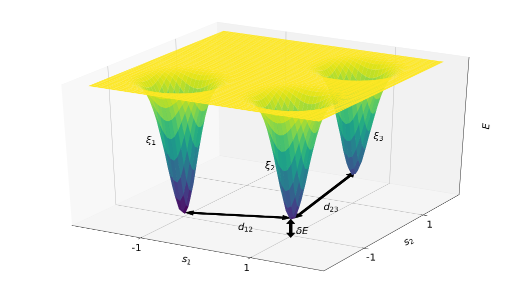
Thus, the description of the dynamical equation given by Eq. (5) on the energy surface given by Eq. (4) is straightforward: one starts with the random (with no prior information) coordinates, which corresponds to either the basin of the planted pattern or spurious state, and then follows the gradient descent until reaching the steady state and consequent projection into corners of the hypercube. The steady state is achieved by compromising between the gradient-descent and slow projection terms (or any other terms, depending on the details of the dynamical equation). Our method distinguishes itself by individually treating the planted minima by separating their (and corresponding mixed states) energies and an additional detailed evaluation of the different dynamical equations’ performance on the produced instances. The schematic picture of this idea and the corresponding energy landscape is shown in Fig. 1.
We present the calculations on different scales and with the different classes of dynamical equations according to our classification, ranging from the simple Hopfield NN to the complicated dynamics with higher derivatives and annealing schedules, part of which are presented in the Supplementary Material section. However, much emphasis will be put on the simplest Eq. (5). Additional information about the classification of dynamical equations and their transformations with the corresponding references are presented in [65, 9].
III Small scale classification
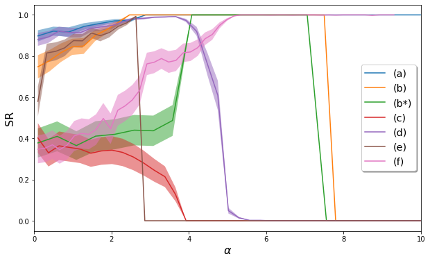
Before describing the construction of the problem instances, it is crucial to make a few comments about the symmetries in our system, which take only quadratic interactions (so-called zero-field Ising Hamiltonian). According to Hebb’s rule, planting a pattern will produce its mirror ”twin” in the phase space, which reflects the mirror symmetry. Thus, changing a sign of all components of some of the planted pattern will not affect the energy landscape. Moreover, the system has a gauge symmetry, which allows one to reverse particular spins in planted patterns without affecting the complexity of the energy landscape. Nevertheless, such transformations will manifest themselves in the coefficients.
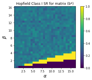
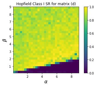
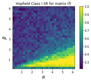
Figure 2 compiles nontrivial SR profiles across all and matrix instances, and captures diverse dynamic behavior of Eq.(5) for finding minimal energy solutions on these matrices. Below, we emphasize the essential role of matrix choice, explore inter-matrix differences, delve into parametrization details, and outline our complexity framework.
We introduce a few small-scale matrices with the corresponding classification on which the presented dynamical systems were tested and showed various behaviours. For such size, the essential parameters are the number of planted patterns ( in the majority of the cases, so that it is easy to observe the planted patterns and their spurious states without additional effects), Hamming distances between the discrete patterns (or their overlaps), and the value of the asymmetry coefficient , which should be small enough not to affect the patterns basins of attraction. In case of large pattern overlaps, the patterns tend to merge into one global minimum, and the same effect can be achieved by increasing the asymmetry coefficient. Thus, it is reasonable to classify instances by the triplet of the mutual distances between the planted patterns , which produce several possible combinations, the number of which is constrained by the triangle inequality and possible distances . The list of nontrivial configurations is following: a) with , b) with , b∗) with , c) with , d) with , e) with (with the last pattern having the biggest weight) and specific exceptional example with four patterns f) with four equidistant vectors and (to test the complexity beyond the given classification). Other combinations possess trivial properties, e.g. distances are too small, which results in the patterns merging into one global minimum. From the geometrical perspectives, the set of patterns distances uniquely defines the basins of attraction for planted patterns and their mixed combinations and hence the energy landscape, which is also proven by Fig. 2. Such instances are good for testing both algorithms and hardware properties.
In case of the limited capabilities or constraints imposed by the analogue nature of the hardware, the produced matrices can be coarse-grained into another set by the following transformation (depending on the reasonable choice of the discretization parameter ) and preserve the same geometrical properties of the energy landscape and thus complexity (which was verified with the corresponding numerical simulations). One can tune the set by changing the parameter, which depends on the analogue hardware properties and its working precision [19].
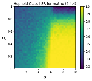
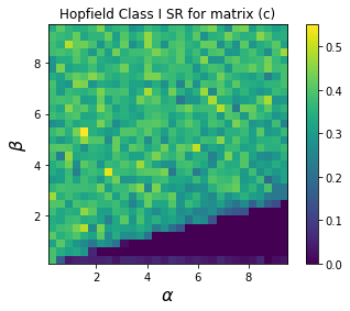
The numerical evolution of Eq. (5) on the given instances gives different results. For small-scale instances, we define the complexity through Success rate (SR) which is the ratio of the runs that reached the ground state to all runs by a particular algorithm for a given instance. The absence of the region with SR is treated as a hard instance, which is the case of the (c) matrix. Easier matrices have all a larger region with SR= or larger SR over all parameters. In the case of (c) instance, we want to effectively ”hide” the ground state by placing other patterns closer to each other to merge into another minimum, which still does not exceed the ground state energy. Thus, the system’s dynamic behaviour will follow the eigenvector of the coupling matrix with the highest eigenvalue, which results from the second and third pattern interaction and does not coincide with the ground state pattern. This means the impossibility of reaching the lowest energy from any point of the phase space, except from the initial conditions very close to it. Using Eq. (4) for defining the energy landscape, we can guarantee that the ground state corresponds to the pattern with the highest asymmetry coefficient, which is the principle eigenvalue of the . Thus, increasing the projection strength fixes the threshold below which the corresponding projections will converge to zero. Increasing further turns the dynamical equations into a trivial fast projection of the initial state, which does not correlate with the ground state. The detailed SR diagrams for all instances (except (e), which is close to the (b) matrix) and statistics for other dynamical equations can be found in the Supplementary Material.
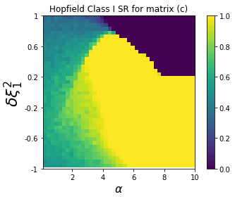
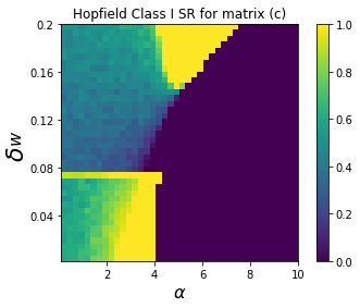
Another noteworthy aspect involves the emergence of complexity transitions within a singular model, that are shown in Fig. 3. Our approach entails the exploration of diverse parameterizations for the model, as defined by the equation Eq. (4). This parameterization has the following form:
| (6) |
We start with the type (c) matrix since it has a complex profile without reaching SR.
The left part of Fig. 3 shows the transition between the states, where we continuously changed the second coordinate of the first pattern in (c) matrix (or any other coordinate which shares a sign across planted patterns) from its original value to the opposite (which corresponds to the going from to ), while keeping other spins constant. Such a procedure effectively changes the distances between patterns, which affects coefficients and hence the complexity of the current instance. As seen in the left part of Fig. 3, the first transition happens with the appearance of the yellow region, which makes the generated instance easy (), while the second is marked by the disappearance of the region with the SR (). In our context, we call the instance ”easy” if its SR diagram possesses region with SR. The middle part of Fig. 3 shows the same (c) matrix SR diagram but with different asymmetry coefficients. Increasing from its original value leads to the dominance of the pattern with the largest weight. Decreasing it also leads to complexity reduction with sharp boundaries.
The right part of Fig. 3 shows the diagram for the specific modification of the equidistant planted patterns with and (index stands for the spin that has a common sign for first two patterns), which becomes hard through the described transition. Even with such a small shift, it is possible to obtain a complexity phase transition, imposed by current parametrization. However, the boundaries are rather smooth, in contrast to the previously described cases. All SR diagrams can be explained through the scope of individual trajectories of Eq. (5) on the landscape defined by Eq. (6). In summary, we introduced various instances of coupling matrices for the QUBO problem of size and systemized them based on the mutual distances. We then demonstrated various ways to modify these instances affecting their complexity. These methods can be used for larger matrices.
 |
 |
 |
IV Numerical results for large N
The transition to the larger allows one to plant more patterns, which leads to more sophisticated scenarios and effects. However, one has to modify the criteria for the hardness of a matrix because of the increasing difficulty of finding the true ground state across all the possible solutions dominated by spurious patterns. Thus, we shift our attention to other characteristics, like the functional form of the final solutions distribution, its dependency on the number of planted patterns, and the distribution of found energies relative to the planted ones.
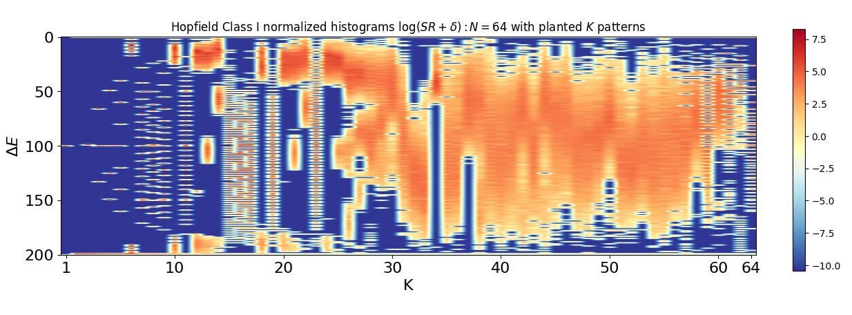
Dimension produces quite a reasonable space for planting many patterns. We perform extensive numerical simulations of Eq. (5) over the instances defined by the coupling matrices of Eq. (4) for each with (where is the principal eigenvalue of the coupling matrix) until the steady state is found. For initial conditions, we use vectors with independent random coordinates uniformly distributed in the interval , with small enough . Although it is costly to characterise the entire phase space, we perform an appropriate sampling, enough to characterize the energy landscape. After reaching the steady state, we calculate the energy according to Eq. (1), normalise it using the maximal and minimal found energy values and plot in the Fig. 5.
To highlight the shape of the empirical energy distribution, Fig. 5 shows the smoothed histograms centred between the maximal and minimal empirically found energy values, demonstrating a variety of scenarios. There are few notable regimes, depending on the number of the planted patterns . For small , there are separated planted patterns with their mirror copies and spurious states. For moderate : , the number of found spurious states becomes bigger, resulting in the cluster’s appearance and multimodal distributions, sometimes mixed with the sparse histograms of the same spurious states. For large the dominance of the spurious states becomes evident, resulting in the distributions being close to normal until reaching the saturated regime , where the distributions become trivial again. Such trivialization can be explained. Taking equal weights as in the original Hebb’s rule and placing the orthogonalized patterns will produce the matrix with zero off-diagonal elements [5]. Thus, taking in Eq. (4) effectively renormalizes the weights into , because terms with the cancel each other, leaving weights with linear dependency on , which has an exponential impact on the dynamics of convergence to a particular pattern. The complexity of finding the lowest or sub-optimal energy state depends on the complexity parameters: , which regulates the number of local minima, patterns distances between each other (with the orthogonal conditions being the most complex) and asymmetry coefficients (which we do not focus on).
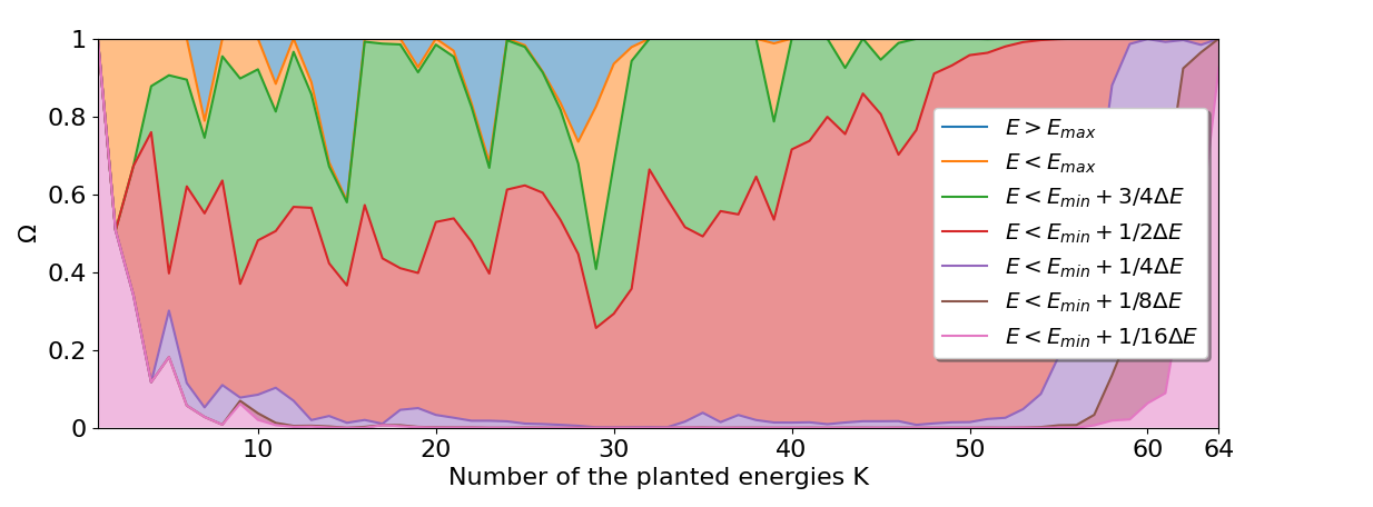
Figure 5 presents the measure of the found solutions’ energies with respect to the planted energies or spectrum. The probability of finding patterns with low enough energies is comparatively low in the primary region , where most obtained energies are localized below the energies mean (red colour). Another significant measure consists of patterns above the mean but below three-quarters of the planted energies range. There are found solutions that lie outside of the given range for some . For other values of or , the dynamics are trivial, and the solutions are closer to the ground state. A more detailed picture can be found in the Supplementary Material.
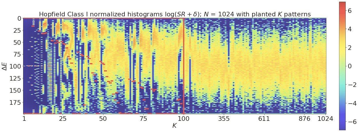
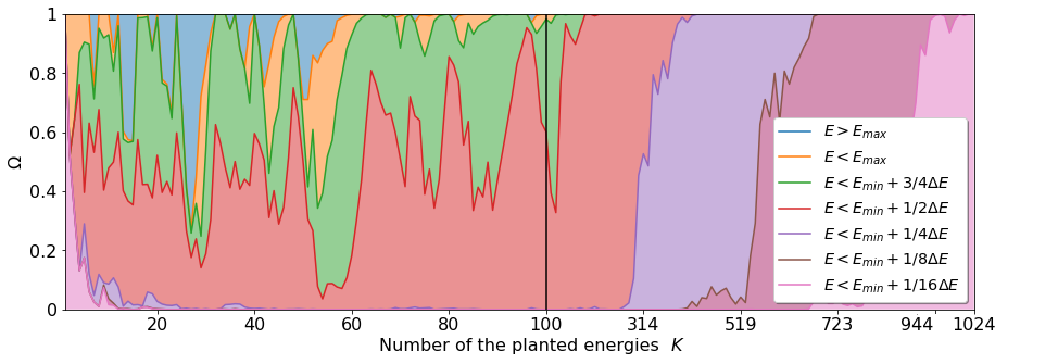
Finally, we perform similar numerical simulations for over the instances defined by Eq. (4) for each with the projection strength equals half of the maximal eigenvalue of the matrix and same initial conditions as in case. We perform an appropriate sampling, enough to evaluate various characteristics and their measure, although the amount of runs is less than in the previous case.
To present the distribution form, Fig. 7 shows the histograms centred between the found maximal and minimal energy values. We concentrated on the same indicators as in the previous case. Many patterns appearing, in this case, are similar. For the , the dominance of the spurious states results in close to normal distributions (until the saturated regime). However, such a regime occupies a bigger range of . Therefore, we expect the ratio of the for the starting value of the corresponding regime to be lower with the increase in . For small , there are well separated planted patterns with their mirror copies and spurious states. After , there are mostly cluster and multimodal distributions of minima, which slowly transform close to normal distribution.
Figure 7 presents the measure of the found solutions’ energies with respect to the planted spectrum. In the region , most of the obtained energies are localized below the energies mean (red colour), except for some particular regions, and the distributions are more diverse than in the case. For the higher value of , one can use good approximations for the Gaussian distributions with . Choosing for constructing the matrix instance will possess a problem of reasonable complexity. A more detailed picture can be found in the Supplementary Material Section.
The asymmetry parameters for and for and were picked intentionally small not to affect the basins of attraction. However, this choice leads to a slight numerical difference between found solutions, and one must be careful to differentiate them properly. The choice of the projection strength equals half of the maximal eigenvalue allows one to have a reasonable convergence as well as to obtain a sample of the close to the optimal solutions with the empirical evidence (see the left picture in Fig. S3). However, the projection strength significantly affects the form of the distribution; see the additional plots in the Supplementary Material section.
V Discussion and conclusions
We introduced universal, easy-to-reproduce generative models for the QUBO instances to differentiate the performance of the hardware/solvers. One can use different aspects of such benchmarks. By tuning the complexity, it is possible to determine the performance of the algorithm/hardware on the given instance. Different methods can be compared and contrasted by their probability of reaching the ground state or particular energy interval of sub-optimal solutions. One can also measure the output energy distributions and compare them with the obtained by current numerics. The precise correspondence or mismatch between found energies is an indicator of the difference in methods descriptions or physical principles of unconventional computing. In summary, one can use the whole model, its particular instances or some reproduced patterns with various parameters to compare the hardware performance. We investigated small, medium and large-scale problems and their properties. The described approach is easy to implement and can be successfully applied to benchmark classical and quantum devices. Moreover, our method establishes a prospective platform to characterize the performance of the hardware devices’ physical processes and algorithms for novel computing machines.
Compared to the conventional random matrix ensembles, which are also widely used to perform the optimization, our model has many more local minima and offers higher complexity in finding the optimal or sub-optimal solution (assuming the the method does not incorporate any prior information about the model). Another advantage is the classification of possible states and trajectories, which is statistically hard to describe for the fully random instances.
The presented approach lies at the intersection of many fields, such as tensor factorization (since Eq. (2) is essentially rank decomposition of a matrix) [66] or statistical physics and dynamics of complex systems [44], not to mention that Eq. (5) (and its modifications) is the Hopfield equations [41, 60], the simplest form of the NN.
VI Supplementary Material
This Section contains supplementary information and additional numerical results. We present the calculations on different scales and with the different classes of dynamical equations according to our classification, which is presented below, ranging from the simple Hopfield NN to the complicated dynamics with higher derivatives and annealing schedules. Class II equations differ from the previous class by the presence of time dependence in its coefficients:
| (7) |
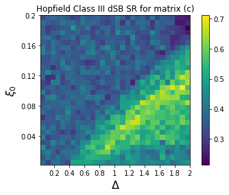
The class III equations have the following form:
| (8) |
and are governed by second-order partial differential equations with time-dependent coefficients, which is the special case of the coupled microelectromechanical systems (MEMs) equations [67]. Similar equations describe bifurcation machines [68, 69, 70]:
| (9) |
where is the positive detuning frequency between the oscillator and pumping frequency, is the external pumping parametrization and is a positive constant with the dimension of frequency from the original model [68]. The clear analogy between different parametrization of Eq. (9) and Eq. (8) is following and (with ). However, all the equations describing various dynamical rules have many connections, with possible transformations between each other [65, 9].
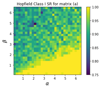
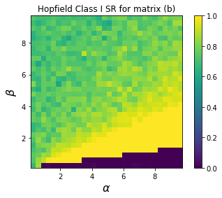
Although for the class I algorithm SR depends only on (or just , assuming ), we plot an additional axis to ensure no numerical mistake. Thus SR is constant across any linear ratio , see Fig. S1 and Fig. S2.
Additional numerical results include left and middle plots in Fig. S3 that shows the gain in the SR by a transition to more complicated dynamics of Eq. (9). The right plot in Fig. S3 shows the dynamics of Eq. (5) algorithm on the average instance of a symmetric random matrix of size , which typically does not have a region with the SR. This diagram can guide the choice of optimal projection strength .
 |
 |
 |
 |
 |
 |
 |
 |
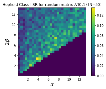 |
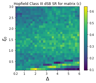
Fig. S4 shows the change in the SR diagrams for Eq. (8) algorithm on the (c) matrix depending on the choice of the threshold argument value.
 |
 |
 |

Figs. S5 and S6 focus on a more detailed picture of the results, presented in the main text, providing additional information about the measure of the particular solutions found.

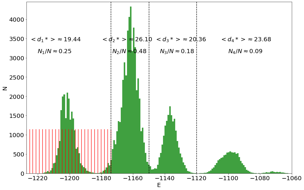
Fig. S7 shows an additional instance of the calculations, i.e. energy histograms for out of the for , demonstrating the multimodal distribution which is the result of the interplay between GD-dynamics and discrete projection.
Additional plots in Figs. S8, S9, S10, S11 present the numerical simulation results to show the influence of both the projection strength and number of the planted patterns on the form of the obtained distributions.


Acknowledgements.
N.G.B acknowledges the support from the Julian Schwinger Foundation JSF-19-02-0005 and Horizon Europe 10086022. N.D. acknowledges the support from the Israel Science Foundation grant No. 1520/22 and ISF-NSFC grant 3652/21.References
- [1] I. Dunning, S. Gupta, and J. Silberholz, “What works best when? a systematic evaluation of heuristics for max-cut and qubo,” INFORMS Journal on Computing, vol. 30, no. 3, pp. 608–624, 2018.
- [2] G. Kochenberger, J.-K. Hao, F. Glover, M. Lewis, Z. Lü, H. Wang, and Y. Wang, “The unconstrained binary quadratic programming problem: a survey,” Journal of combinatorial optimization, vol. 28, no. 1, pp. 58–81, 2014.
- [3] A. Lucas, “Ising formulations of many np problems,” Frontiers in physics, p. 5, 2014.
- [4] S. Mücke, N. Piatkowski, and K. Morik, “Learning bit by bit: Extracting the essence of machine learning.,” in LWDA, pp. 144–155, 2019.
- [5] J. Hertz, A. Krogh, and R. G. Palmer, Introduction to the theory of neural computation. CRC Press, 2018.
- [6] P. Minzioni, C. Lacava, T. Tanabe, J. Dong, X. Hu, G. Csaba, W. Porod, G. Singh, A. E. Willner, A. Almaiman, et al., “Roadmap on all-optical processing,” Journal of Optics, vol. 21, no. 6, p. 063001, 2019.
- [7] D. Woods and T. J. Naughton, “Optical computing,” Applied Mathematics and Computation, vol. 215, no. 4, pp. 1417–1430, 2009.
- [8] H. Wu and Q. Dai, “Artificial intelligence accelerated by light,” 2021.
- [9] N. Stroev and N. G. Berloff, “Analog photonics computing for information processing, inference, and optimization,” Advanced Quantum Technologies, p. 2300055, 2023.
- [10] N. G. Berloff, M. Silva, K. Kalinin, A. Askitopoulos, J. D. Töpfer, P. Cilibrizzi, W. Langbein, and P. G. Lagoudakis, “Realizing the classical xy hamiltonian in polariton simulators,” Nature materials, vol. 16, no. 11, p. 1120, 2017.
- [11] K. P. Kalinin and N. G. Berloff, “Networks of non-equilibrium condensates for global optimization,” New Journal of Physics, vol. 20, no. 11, p. 113023, 2018.
- [12] M. Nixon, M. Friedman, E. Ronen, A. A. Friesem, N. Davidson, and I. Kanter, “Synchronized cluster formation in coupled laser networks,” Physical review letters, vol. 106, no. 22, p. 223901, 2011.
- [13] V. Pal, C. Tradonsky, R. Chriki, A. A. Friesem, and N. Davidson, “Observing dissipative topological defects with coupled lasers,” Physical review letters, vol. 119, no. 1, p. 013902, 2017.
- [14] C. Tradonsky, O. Raz, V. Pal, R. Chriki, A. A. Friesem, and N. Davidson, “Rapid phase retrieval by lasing,” arXiv preprint arXiv:1805.10967, 2018.
- [15] P. L. McMahon, A. Marandi, Y. Haribara, R. Hamerly, C. Langrock, S. Tamate, T. Inagaki, H. Takesue, S. Utsunomiya, K. Aihara, et al., “A fully programmable 100-spin coherent ising machine with all-to-all connections,” Science, vol. 354, no. 6312, pp. 614–617, 2016.
- [16] R. Hamerly, T. Inagaki, P. L. McMahon, D. Venturelli, A. Marandi, T. Onodera, E. Ng, C. Langrock, K. Inaba, T. Honjo, et al., “Experimental investigation of performance differences between coherent ising machines and a quantum annealer,” Science advances, vol. 5, no. 5, p. eaau0823, 2019.
- [17] F. Böhm, T. Inagaki, K. Inaba, T. Honjo, K. Enbutsu, T. Umeki, R. Kasahara, and H. Takesue, “Understanding dynamics of coherent ising machines through simulation of large-scale 2d ising models,” Nature communications, vol. 9, no. 1, p. 5020, 2018.
- [18] D. Pierangeli, G. Marcucci, and C. Conti, “Large-scale photonic ising machine by spatial light modulation,” Physical Review Letters, vol. 122, no. 21, p. 213902, 2019.
- [19] G. Mourgias-Alexandris, H. Ballani, N. G. Berloff, J. H. Clegg, D. Cletheroe, C. Gkantsidis, I. Haller, V. Lyutsarev, F. Parmigiani, L. Pickup, et al., “Analog iterative machine (aim): using light to solve quadratic optimization problems with mixed variables,” arXiv preprint arXiv:2304.12594, 2023.
- [20] N. Stroev and N. G. Berloff, “Discrete polynomial optimization with coherent networks of condensates and complex coupling switching,” Physical Review Letters, vol. 126, no. 5, p. 050504, 2021.
- [21] D. A. Chermoshentsev, A. O. Malyshev, E. S. Tiunov, D. Mendoza, A. Aspuru-Guzik, A. K. Fedorov, and A. I. Lvovsky, “Polynomial unconstrained binary optimisation inspired by optical simulation,” arXiv preprint arXiv:2106.13167, 2021.
- [22] E. S. Tiunov, A. E. Ulanov, and A. Lvovsky, “Annealing by simulating the coherent ising machine,” Optics express, vol. 27, no. 7, pp. 10288–10295, 2019.
- [23] K. P. Kalinin and N. G. Berloff, “Computational complexity continuum within ising formulation of np problems,” Communications Physics, vol. 5, no. 1, pp. 1–10, 2022.
- [24] L. Zdeborová, “Statistical physics of hard optimization problems,” arXiv preprint arXiv:0806.4112, 2008.
- [25] L. Zdeborová and F. Krzakala, “Statistical physics of inference: Thresholds and algorithms,” Advances in Physics, vol. 65, no. 5, pp. 453–552, 2016.
- [26] I. P. Gent and T. Walsh, “The sat phase transition,” in ECAI, vol. 94, pp. 105–109, PITMAN, 1994.
- [27] B. Aubin, A. Maillard, F. Krzakala, N. Macris, L. Zdeborová, et al., “The committee machine: Computational to statistical gaps in learning a two-layers neural network,” Advances in Neural Information Processing Systems, vol. 31, 2018.
- [28] F. Gerace, B. Loureiro, F. Krzakala, M. Mézard, and L. Zdeborová, “Generalisation error in learning with random features and the hidden manifold model,” in International Conference on Machine Learning, pp. 3452–3462, PMLR, 2020.
- [29] F. Hamze, J. Raymond, C. A. Pattison, K. Biswas, and H. G. Katzgraber, “Wishart planted ensemble: A tunably rugged pairwise ising model with a first-order phase transition,” Physical Review E, vol. 101, no. 5, p. 052102, 2020.
- [30] F. Hamze, D. C. Jacob, A. J. Ochoa, D. Perera, W. Wang, and H. G. Katzgraber, “From near to eternity: spin-glass planting, tiling puzzles, and constraint-satisfaction problems,” Physical Review E, vol. 97, no. 4, p. 043303, 2018.
- [31] F. Krzakala and L. Zdeborová, “Statistical physics methods in optimization and machine learning,” 2021.
- [32] A. Abbaras, B. Aubin, F. Krzakala, and L. Zdeborová, “Rademacher complexity and spin glasses: A link between the replica and statistical theories of learning,” in Mathematical and Scientific Machine Learning, pp. 27–54, PMLR, 2020.
- [33] J. Barbier, F. Krzakala, N. Macris, L. Miolane, and L. Zdeborová, “Optimal errors and phase transitions in high-dimensional generalized linear models,” Proceedings of the National Academy of Sciences, vol. 116, no. 12, pp. 5451–5460, 2019.
- [34] F. Krzakala, M. Mézard, F. Sausset, Y. Sun, and L. Zdeborová, “Probabilistic reconstruction in compressed sensing: algorithms, phase diagrams, and threshold achieving matrices,” Journal of Statistical Mechanics: Theory and Experiment, vol. 2012, no. 08, p. P08009, 2012.
- [35] D. L. Donoho, A. Maleki, and A. Montanari, “Message-passing algorithms for compressed sensing,” Proceedings of the National Academy of Sciences, vol. 106, no. 45, pp. 18914–18919, 2009.
- [36] T. Aonishi, K. Mimura, M. Okada, and Y. Yamamoto, “L0 regularization-based compressed sensing with quantum-classical hybrid approach,” Quantum Science and Technology, 2022.
- [37] D. Gamarnik, “The overlap gap property: A topological barrier to optimizing over random structures,” Proceedings of the National Academy of Sciences, vol. 118, no. 41, p. e2108492118, 2021.
- [38] D. Gamarnik, C. Moore, and L. Zdeborová, “Disordered systems insights on computational hardness,” Journal of Statistical Mechanics: Theory and Experiment, vol. 2022, no. 11, p. 114015, 2022.
- [39] J.-G. Liu, X. Gao, M. Cain, M. D. Lukin, and S.-T. Wang, “Computing solution space properties of combinatorial optimization problems via generic tensor networks,” arXiv preprint arXiv:2205.03718, 2022.
- [40] D. O. Hebb, “Organization of behavior. new york: Wiley,” J. Clin. Psychol, vol. 6, no. 3, pp. 335–307, 1949.
- [41] J. J. Hopfield, “Neural networks and physical systems with emergent collective computational abilities.,” Proceedings of the national academy of sciences, vol. 79, no. 8, pp. 2554–2558, 1982.
- [42] M. J. Schuetz, J. K. Brubaker, and H. G. Katzgraber, “Combinatorial optimization with physics-inspired graph neural networks,” Nature Machine Intelligence, vol. 4, no. 4, pp. 367–377, 2022.
- [43] M. Mohseni, D. Eppens, J. Strumpfer, R. Marino, V. Denchev, A. K. Ho, S. V. Isakov, S. Boixo, F. Ricci-Tersenghi, and H. Neven, “Nonequilibrium monte carlo for unfreezing variables in hard combinatorial optimization,” arXiv preprint arXiv:2111.13628, 2021.
- [44] L. P. Kadanoff, Statistical physics: statics, dynamics and renormalization. World Scientific, 2000.
- [45] B. A. Wilson, Z. A. Kudyshev, A. V. Kildishev, S. Kais, V. M. Shalaev, and A. Boltasseva, “Machine learning framework for quantum sampling of highly constrained, continuous optimization problems,” Applied Physics Reviews, vol. 8, no. 4, p. 041418, 2021.
- [46] V. Ros and Y. V. Fyodorov, “The high-d landscapes paradigm: spin-glasses, and beyond,” arXiv preprint arXiv:2209.07975, 2022.
- [47] P. G. Wolynes, “Landscapes, funnels, glasses, and folding: From metaphor to software,” Proceedings of the American Philosophical Society, vol. 145, no. 4, pp. 555–563, 2001.
- [48] R. H. Austin, “Free energies, landscapes, and fitness in evolution dynamics,” in Quantitative Biology: From Molecular to Cellular Systems, pp. 1–21, CRC Press, 2012.
- [49] P. Krugman, “Complex landscapes in economic geography,” The American Economic Review, vol. 84, no. 2, pp. 412–416, 1994.
- [50] M. Goldstein, “Viscous liquids and the glass transition: a potential energy barrier picture,” The Journal of Chemical Physics, vol. 51, no. 9, pp. 3728–3739, 1969.
- [51] D. O. Hebb, The organization of behavior: A neuropsychological theory. Psychology Press, 2005.
- [52] W. A. Little, “The existence of persistent states in the brain,” Mathematical biosciences, vol. 19, no. 1-2, pp. 101–120, 1974.
- [53] D. Krotov and J. J. Hopfield, “Dense associative memory for pattern recognition,” Advances in neural information processing systems, vol. 29, 2016.
- [54] H. Ramsauer, B. Schäfl, J. Lehner, P. Seidl, M. Widrich, T. Adler, L. Gruber, M. Holzleitner, M. Pavlović, G. K. Sandve, et al., “Hopfield networks is all you need,” arXiv preprint arXiv:2008.02217, 2020.
- [55] S. Chen, G. Huang, G. Piccioli, and L. Zdeborová, “Planted x y model: Thermodynamics and inference,” Physical Review E, vol. 106, no. 5, p. 054115, 2022.
- [56] D. Perera, I. Akpabio, F. Hamze, S. Mandra, N. Rose, M. Aramon, and H. G. Katzgraber, “Chook–a comprehensive suite for generating binary optimization problems with planted solutions,” arXiv preprint arXiv:2005.14344, 2020.
- [57] I. Hen, J. Job, T. Albash, T. F. Rønnow, M. Troyer, and D. A. Lidar, “Probing for quantum speedup in spin-glass problems with planted solutions,” Physical Review A, vol. 92, no. 4, p. 042325, 2015.
- [58] J. Dong, L. Valzania, A. Maillard, T.-a. Pham, S. Gigan, and M. Unser, “Phase retrieval: From computational imaging to machine learning: A tutorial,” IEEE Signal Processing Magazine, vol. 40, no. 1, pp. 45–57, 2023.
- [59] A. Maillard, B. Loureiro, F. Krzakala, and L. Zdeborová, “Phase retrieval in high dimensions: Statistical and computational phase transitions,” Advances in Neural Information Processing Systems, vol. 33, pp. 11071–11082, 2020.
- [60] J. J. Hopfield and D. W. Tank, ““neural” computation of decisions in optimization problems,” Biological cybernetics, vol. 52, no. 3, pp. 141–152, 1985.
- [61] J. M. Kosterlitz, D. J. Thouless, and R. C. Jones, “Spherical model of a spin-glass,” Physical Review Letters, vol. 36, no. 20, p. 1217, 1976.
- [62] M. Mézard, G. Parisi, and M. A. Virasoro, Spin glass theory and beyond: An Introduction to the Replica Method and Its Applications, vol. 9. World Scientific Publishing Company, 1987.
- [63] V. S. Dotsenko, M. Feigel’man, and L. Ioffe, Spin glasses and related problems, vol. 1. CRC Press, 1990.
- [64] S. N. Majumdar and G. Schehr, “Top eigenvalue of a random matrix: large deviations and third order phase transition,” Journal of Statistical Mechanics: Theory and Experiment, vol. 2014, no. 1, p. P01012, 2014.
- [65] M. Syed and N. G. Berloff, “Physics-enhanced bifurcation optimisers: All you need is a canonical complex network,” arXiv preprint arXiv:2207.11256, 2022.
- [66] A. Cichocki, R. Zdunek, A. H. Phan, and S.-i. Amari, Nonnegative matrix and tensor factorizations: applications to exploratory multi-way data analysis and blind source separation. John Wiley & Sons, 2009.
- [67] F. C. Hoppensteadt and E. M. Izhikevich, “Synchronization of mems resonators and mechanical neurocomputing,” IEEE Transactions on Circuits and Systems I: Fundamental Theory and Applications, vol. 48, no. 2, pp. 133–138, 2001.
- [68] H. Goto, K. Tatsumura, and A. R. Dixon, “Combinatorial optimization by simulating adiabatic bifurcations in nonlinear hamiltonian systems,” Science advances, vol. 5, no. 4, p. eaav2372, 2019.
- [69] H. Goto, K. Endo, M. Suzuki, Y. Sakai, T. Kanao, Y. Hamakawa, R. Hidaka, M. Yamasaki, and K. Tatsumura, “High-performance combinatorial optimization based on classical mechanics,” Science Advances, vol. 7, no. 6, p. eabe7953, 2021.
- [70] T. Kanao and H. Goto, “Simulated bifurcation assisted by thermal fluctuation,” arXiv preprint arXiv:2203.08361, 2022.