Evaluating a Sigmoid Dark Energy Model to Explain the Hubble Tension

Abstract

In this study we analyze Type Ia supernovae (SNe Ia) data sourced from the Pantheon+ compilation [6] to investigate late-time physics effects influencing the expansion history, $H(z)$, at redshifts $(z<2)$. Our focus centers on a time-varying dark energy (DE) model that introduces a rapid transition in the equation of state, at a specific redshift, $z_{a}$, from the baseline, $\Lambda=-1$, value to the present value, $w_{0}$, through the implementation of a sigmoid function. The constraints obtained for the DE sigmoid phenomenological parametrization have broad applicability for dynamic DE models that invoke late-time physics. Our analysis indicates that the sigmoid model provides a slightly better, though not statistically significant, fit to the SNe Pantheon+ data compared to the standard $\Lambda CDM$ alone. The fit results, assuming a flat geometry and maintaining $\Omega_{m}$ constant at the 2018-Planck value of $0.3153$, are as follows: $H_{0}=73.3^{+0.2}_{-0.6}$  km s^-1 Mpc^-1 , $w_{0}=-0.95^{+0.15}_{-0.02}$, $z_{a}=0.8\pm 0.46$. The errors represent statistical uncertainties only. The available SN dataset lacks sufficient statistical power to distinguish between the baseline $\Lambda CDM$ and the alternative sigmoid models. A feature of interest offered by the sigmoid model is that it identifies a specific redshift, $z_{a}=0.8$, where a potential transition in the equation of state could have occurred. The sigmoid model does not favor a DE in the phantom region ($w_{0}<-1$). Further constraints to the dynamic DE model have been obtained using CMB data to compute the distance to the last scattering surface. While the sigmoid DE model does not completely resolve the $H_{0}$ tension, it offers a transition mechanism that can still play a role alongside other potential solutions.

1 Introduction

The Hubble tension denotes the disparity between the values of the Hubble constant, $H_{0}$, derived from cosmic microwave background (CMB) data and those measured using the magnitude-redshift relation with data from standard candles such as Type Ia Supernovae (SNe Ia) [2]. The reported value of $H_{0}=73.04\pm 1.04$  km s^-1 Mpc^-1 based on SNe Ia [5, hereafter R22] and $H_{0}=67.36\pm 0.54$  km s^-1 Mpc^-1 derived from CMB [4, hereafter Planck-2018], results in a discrepancy at the $4.9\sigma$ level of significance. For simplicity, the units of $H_{0}$ are omitted hereafter (assume  km s^-1 Mpc^-1). It is important to clarify that the Planck results for $H_{0}$ are not a direct measurement but a model-dependent inference, assuming a flat $\Lambda$-cold dark matter ($\Lambda CDM$) cosmology.

While local values of $H_{0}$, such as those presented in R22, are model-independent, those derived from CMB depend on physics in the early universe $(z\approx 1000)$. Consequently, the challenge presented by the Hubble tension lies in finding models that preserve the CMB results while allowing for a transition to higher $H_{0}$ values at low redshifts. This observation motivates the exploration of late-time physics effects, which introduce deviations from the standard $\Lambda CDM$ model and could potentially elucidate the $H_{0}$ tension.

We investigate a scenario involving a time-varying dark energy (DE) equation of state (EOS) as a mechanism capable of introducing deviations from the standard $\Lambda CDM$ model. From an observational standpoint, dynamic DE models can be directly incorporated into the calculation of distances to SNe used in the data fits.

In the $\Lambda CDM$ model, acceleration is driven by a cosmological constant $\Lambda$ with an EOS, $w=P/\rho=-1$, where $P$ represents pressure and $\rho$ represents density, both in energy equivalent units to ensure a dimensionless ratio. In this model, the expansion history, $H(z)$, exhibits a gradual evolution profile from deceleration $(z>0.7)$ to acceleration $(z<0.7)$. However, this alone fails to account for the higher $H_{0}$ values derived from SN data.

The Chevallier-Polarski-Linder (CPL) dynamic DE model [3], proposes a simple parametrization for the equation of state involving a linear change with the cosmological scale factor, $a$: $w(a)=w_{0}+w_{a}(1-a)$, where $w_{0}$ represents the current value, and $w_{a}$ the negative slope. It has been demonstrated [7] that the CPL model suffers from significant parameter degeneracy, limiting its ability to explain the tension. Moreover, the deviations from the standard $\Lambda CDM$ that CPL allows extend over a wide range in redshift space, restricting the model’s capacity to capture changes in the EOS at specific redshifts.

To address these challenges, we focus on a DE model that introduces a change in the expansion history H(z) (relative to $\Lambda CDM$) activated at a specific redshift, $z_{a}$. The advantage of this late DE model lies in its ability to incorporate a transition at a specific redshift, thus meeting the requirement to preserve early CMB physics. It is worth noting that the proposed sigmoid model serves as a physics-agnostic phenomenological parametrization useful for constraining physical models. Examples of such models include a scalar field undergoing a phase transition akin to inflation.

2 The Sigmoid Dark Energy Model

The analysis presented in R22 relies on a subset of the Pantheon+ dataset, consisting of low-redshift SN with $z<0.15$, providing a measurement of the local value of $H_{0}$. In this redshift range, the Hubble law is evident in a straightforward plot of magnitude versus $\log cz$, with the Hubble constant given by the intercept, $a_{B}$: $\log H_{0}=5+M/5-a_{B}/5$, where M signifies the fiducial SN Ia luminosity. R22’s analysis involves calibration parameters in addition to the magnitude-redshift relationship.

Given R22’s focus on low-redshift, the approximation for distance at these redshifts is appropriate. However, when extending the analysis to higher redshifts, an accurate formula for distance becomes crucial. Hence, for analysis purposes, it is convenient to categorize the redshift space into three regions: local, $z<0.15$, as utilized in R22, Hubble Flow (HF), $0.15<z<2.3$, determined by the depth of the Pantheon+ dataset, and high-redshift, $z\approx 2.3$.

Fitting models to SNe data in the HF and high-redshift regions requires model-dependent distance computations. The magnitude, $m_{B}$, is linked to distance through the equation:

$$m_{B}=25+M+5\log{d_{L}\left(z\right)}$$ (1)

Here, $M$ represents the absolute magnitude of Type Ia supernovae, whith R22 determining a value of $M=-19.253$. The luminosity distance, $d_{L}$, expressed in Mpc units, is model dependent, and for a flat spatial geometry, $\Omega_{k}=0$, is given by:

$$d_{L}(z)=\frac{c(1+z)}{H_{0}}\int_{0}^{z}\frac{1}{\sqrt{\Omega_{r}(1+z^{\prime})^{4}+\Omega_{M}(1+z^{\prime})^{3}+\Omega_{\Lambda}f(z^{\prime})}}dz^{\prime}$$ (2)

where $f(z)$ encapsulates the dependence on the dynamic DE model. The $\Omega_{x}$ parameters denote the standard density parameters for radiation, $r$, matter, $M$ and dark energy, $\Lambda$.

The dynamic DE model proposed in this study, employs a sigmoid function to describe the dark energy equation of state, $w(z)$, transitioning from $w_{a}=-1$ for $z>z_{a}$ to $w_{0}$ for $z<z_{a}$, as follows:

$$w(z)=w_{0}+\frac{w_{a}-w_{0}}{1+e^{\left(\frac{z_{a}-z}{r}\right)}}$$ (3)

The equation above describes a smooth transition taking place at a redshift centered around $z_{a}$ with a transition rate $r$. The value of $w_{a}$ is set to $-1$ to ensure that at high redshifts the universe’s dynamics adhere to the standard $\Lambda CDM$, with $\Lambda$ serving as the source of DE. This choice preserves the CMB results. The parameter $r$ is fixed to $0.125$ to model a rapid transition (a feature of the model).

The impact of the sigmoid model on the expansion history, $H(z)$, becomes evident when considering the definition of $H(z)$ in the case of spatially flat geometry ($\Omega_{k}=0$). In this context $H(z)$ is expressed as:

$$H(z)=H_{0}\sqrt{\Omega_{r}(1+z)^{4}+\Omega_{M}(1+z)^{3}+\Omega_{\Lambda}f(z)}$$ (4)

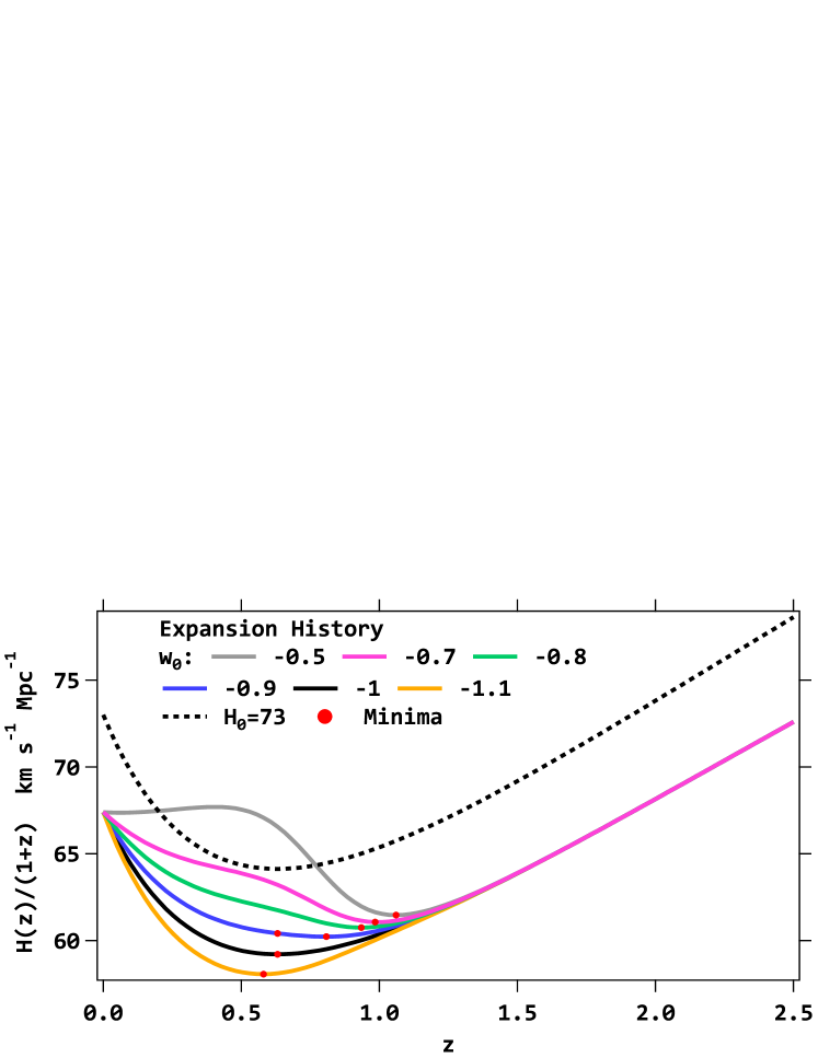
where $f(z)$ represents the dynamic DE term derived from the sigmoid equation of state (Equation 3). Specifically, $f(z)=1$ for $z>z_{a}$, and $f(z)=(1+z)^{3(1+w_{0})}$ for $z<z_{a}$. It is noteworthy that the sigmoid function ensures a smooth transition between these two states. Figure 1 illustrates curves of $H(z)$ for various settings of the $w_{0}$ parameter.

Figure 1: Comoving Hubble parameter as a function of redshift for various settings of the sigmoid parameter $w_{0}$. The other parameters of the model were fixed at $H_{0}=67.4$, $\Omega_{M}=0.3153$, $\Omega_{\Lambda}=1-\Omega_{M}$, and $z_{a}=0.8$. The curve with $w_{0}=-1$ (solid black line) represents the cosmological model with DE provided solely by $\Lambda$. The black dashed line represents the $\Lambda$ model with $H_{0}=73$.

2.1 The Sigmoid Dark Energy Mechanism

The $H_{0}$ parameter in Equation 4 acts as the anchor point at $z=0$, all the $H(z)$ curves originate from this $H_{0}$ anchor point and evolve according to the Friedmann framework. Cosmological parameters, including time-varying DE parameters, do not influence $H_{0}$, but they can modify the shape of $H(z)$ at intermediate redshifts, as evident from the $H(z)$ curves. Changing $H_{0}$ merely shifts the $H(z)$ curves vertically, resulting in the offset observed between the $\Lambda$ model curves (solid and dashed black lines in the figure). The parameter $H_{0}$ plays a similar role in the distance equation (Equation 2), which can be expressed generally as $d_{L}=A/H_{0}$, where A is the integral term containing the cosmological parameters $\Omega_{M}$, $w_{0}$ and $z_{a}$. When this equation is employed in the fits to compare against SNe data, the fitting algorithm’s minima tend to bring the ratio $A/H_{0}$ as close as possible to the data. Consequently, to compensate for an overestimation of the (model-dependent) term $A$, the fit results in an overestimation of $H_{0}$.

In the sigmoid DE model, the mechanism functions as follows: (i) If the true dark energy behavior of the universe followed an actual sigmoid pattern with a parameter $w_{0}>-1$, the distances (and consequently the magnitudes) of SNe in the HF region ($0.15<z<2.3$) would appear smaller than those in a $\Lambda CDM$ universe. (ii) When employing a fitting algorithm using a $\Lambda CDM$ model with SNe observed in our hypothetical true sigmoid universe, the algorithm overestimates the term $A$ in distance calculations. To compensate, it pushes $H_{0}$ to higher values. As a result, the fit outcomes are biased towards higher $H_{0}$ values, partially explaining why the local $H_{0}$ appears higher than the CMB-derived value.

However, even in the most optimistic scenario where the sigmoid model is accurate, we must contend with the fact that the R22 measurement of the local $H_{0}$ is model-independent. The described mechanism could enable the sigmoid model to explain observations of SNe in the HF redshift region, while maintaining a $H_{0}$ value compatible with the CMB-derived value. Nevertheless, additional physics, operating in the $z<0.15$ range, is necessary to bring the value of the local $H_{0}$ closer to the model-independent value measured by R22.

3 Fits to Pantheon+ Data

In the present analysis, we employed a subset of the Pantheon+ SNe compilation [6]. The use of the Pantheon+ offers several advantages: it incorporates cross-calibrations of the various photometric systems utilized in the compilation, the light curves have undergone a self-consistency analysis process, the uncertainties are well characterized with a covariance matrix provided in the data delivery, and the data is consolidated in a properly formatted file accessible to the public. The Pantheon+ dataset has been utilized in recent analyses of the $H_{0}$ tension, such as R22 and [1, hereafter B22].

The Pantheon+ compilation comprises a sample of 1701 light curves from 1550 distinct SNe. For our study, we selected a subset suitable for analysis in the HF region, implementing a redshift cut of $0.0233<z<1.912$ and conducting several data quality checks. The choice of a minimum $z$ value is motivated by the need to exclude the effects of proper motions and potential local void structures. A similar $z_{min}$ criterion was applied in R22 when selecting Pantheon+ data for their HF analysis. Quality checks involved the following criteria: $\sigma_{z}<0.01$, $|c|<0.2$, $|x1|<2.5$ and $\sigma_{m}<0.5$, where $m$ represents SN magnitude, and $c$ and $x1$ denote light-curve fit parameters, for color and shape, respectively. After applying these criteria, the resulting HF sample comprised of 1239 light curves from 1177 distinct SNe. To fit the sigmoid model to the SNe data, we followed the standard Least-Squares $\chi^{2}$ minimization technique using SN magnitude, $m$, and redshift, $z$, as the primary data. The $\chi^{2}$ value was computed as follows:

$$\chi^{2}=\mathbf{R}^{T}\mathbf{C}^{-1}\mathbf{R}$$ (5)

where $\mathbf{C}$ represents the covariance matrix and $\mathbf{R}$ is the residual vector. The covariance matrix, which includes both statistical and systematic uncertainties, is part of the Pantheon+ data release.

The residual vector represents the difference between the data, denoted as $m_{i}$, and the model, denoted as $m_{B}$:

$$R_{i}=m_{i}-m_{B}(z_{i};H_{0},w_{0},z_{a})$$ (6)

where $m_{i}$ is the apparent magnitude of the $i-th$ SNe in the sample, $z_{i}$ its corresponding redshift. The model for SN magnitude $m_{B}$ depends on the sigmoid parameters $(w_{0},z_{a})$, and other cosmological parameters as described in Equation 1.

Planck-2018 established that cosmological parameters are consistent with flat spatial geometry, and the internal consistency of CMB-derived cosmological parameters is tightly constrained (i.e. it is impossible to alter one parameter without breaking consistency). Due to this, $\Omega_{M}$ is kept constant in the fit and set to the Planck-2018 value of $0.3153$, while the flat geometry assumption is retained, $\Omega_{\Lambda}=1-\Omega_{M}-\Omega_{r}$.

The fit was performed using a numerical optimization code employing a line-search step method and finite-differences method for calculating the Hessian. The fit parameters are $H_{0}$, $w_{0}$ and $z_{a}$. The uncertainties associated with the fitted parameters were obtained through a Monte Carlo procedure, as described below and represent statistical errors only. The results of the fit are presented in Table 1 and visually depicted in Figure 2.

Table 1: Fit of the sigmoid and $\Lambda CDM$ models to Pantheon+ SNe data. The errors are statistical only.

Parameter	Sigmoid Fit	$\Lambda CDM$ Fit
$H_{0}$	$73.3^{+0.2}_{-0.6}$	$73.53\pm 0.15$
$w_{0}$	$-0.95^{+0.15}_{-0.02}$
$z_{a}$	$0.81\pm 0.46$
$\chi^{2}/N_{dof}$	$1110.49/1236$	$1111.42/1238$

Figure 2: SNe magnitude data (blue dots, and error bars), best fit (red trace) and residuals.

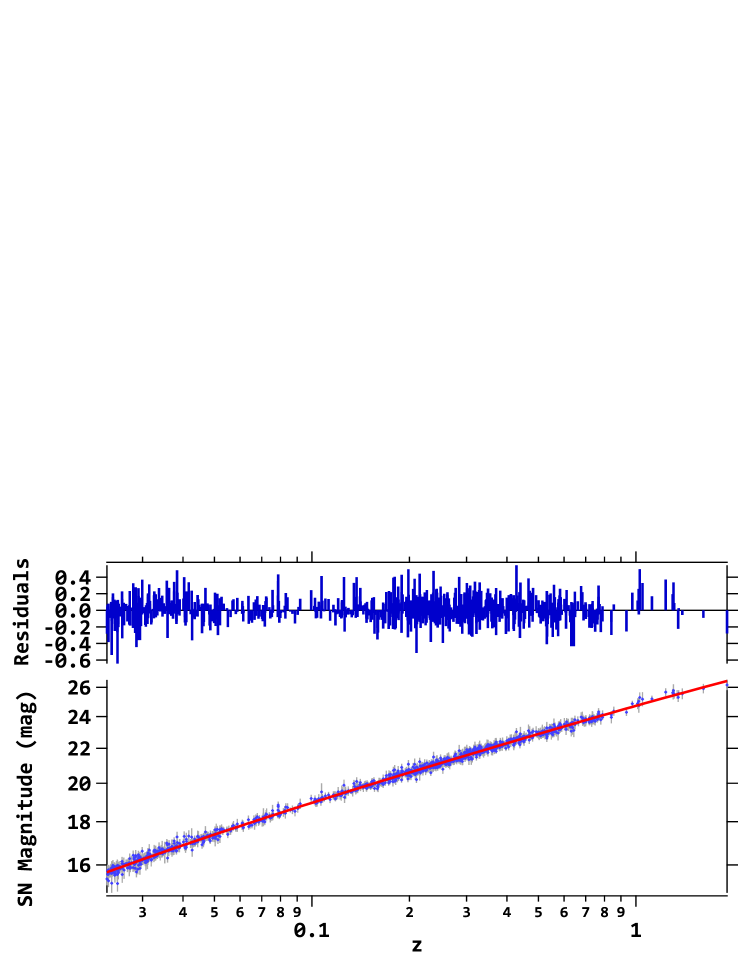
When comparing the fit results presented in Table 1 it is noteworthy that the sigmoid DE model yields a slightly lower value of $\chi^{2}$ relative to the $\Lambda CDM$ model. However, this difference is statistically inconsequential ($0.26\sigma$). The fact that the $\chi^{2}$ values in both fits are smaller than their respective numbers of degrees-of-freedom, $N_{dof}$, renders the $\chi^{2}$ statistic ineffective as a measure of goodness-of-fit. In this case, it is more likely that the $\chi^{2}$ values reflect the effects of correlations in the covariance matrix. In sum, given that for $N_{dof}=1236$ the $\chi^{2}$ has a standard deviation of $\approx\sqrt{2N_{dof}}=49.7$, it is highly probable that such small differences ($0.93$) in the $\chi^{2}$ values are the result of noise alone. Based on these considerations, it is not possible to conclude that the sigmoid model fits the data better than $\Lambda CDM$. However, upon inspecting the residuals, which have an $RMS=0.143$ mag (smaller than the average magnitude error of the sample), it can be stated that the fit is reasonably well (see Figure 2). Therefore, the sigmoid DE model is not ruled out; it can explain the data as effectively as the $\Lambda CDM$ baseline.

The sigmoid function identifies a redshift of $z_{a}=0.8$ as the time in the expansion history when the equation of state transitioned from a cosmological constant, $w=-1$, to $w_{0}=-0.95$. The change in $w$ is small ($0.36\sigma$) and pushes $w$ away from the phantom region ($w<-1$).

3.1 Monte Carlo

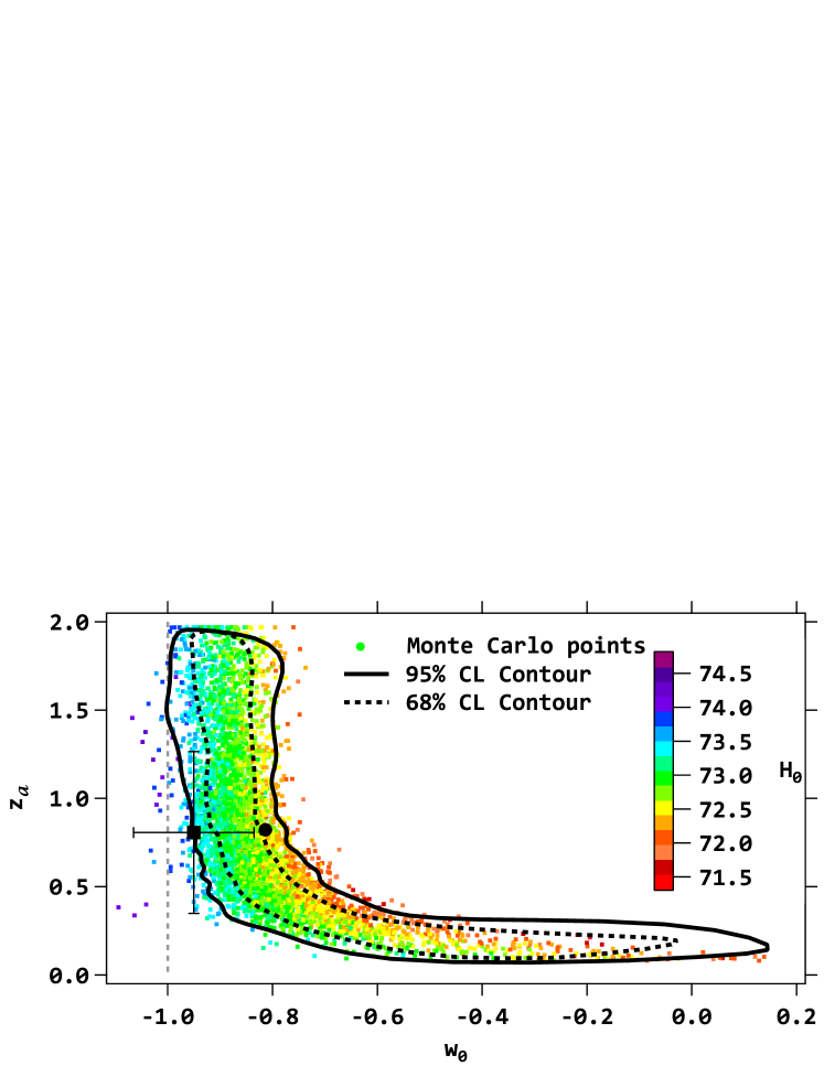
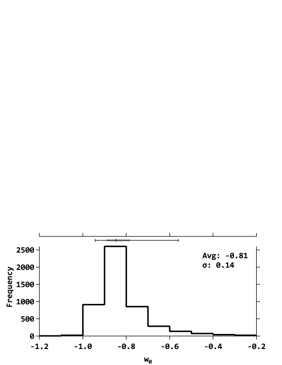
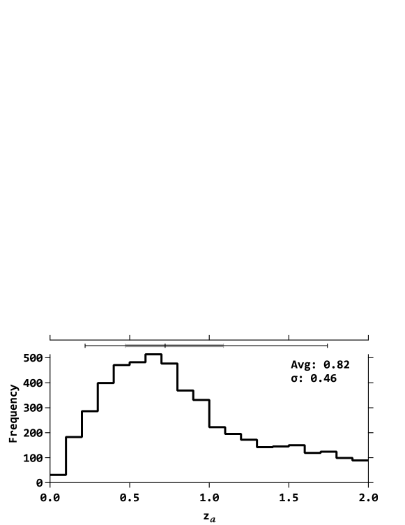
A Monte Carlo code was developed to generate synthetic SNe compilations at the same redshifts as the Pantheon+ SNe subset used in the main fit. For each realization, the Monte Carlo loop generates randomized magnitudes (as per Equation 1) with Gaussian noise of $\sigma_{m}=0.2$ (the average magnitude error), utilizing an underlying DE sigmoid model with true parameters ($w_{0},z_{a}$) set equal to the best fit values (Table 1). Subsequently, the fit code was executed for each realization, resulting in a corresponding set of best-fit $(w_{0},z_{a})$ parameters. The 68% and 95% confidence level (CL) contours of the Monte Carlo points on the $(w_{0},z_{a})$ plane are shown in Figure 3 and the marginalized distributions are presented in Figure 4 and Figure 5.

In Figure 3, the black square with error bars represents the best fit, where the error bars denote the standard deviations of the Monte Carlo data (i.e., marginalized errors), and the black circle corresponds to the mean of the Monte Carlo points. The relative displacement between these two reference points indicates a small bias ($0.037$) in $w_{0}$. The contour plot illustrates a distinct degeneracy structure in the ($w_{0},z_{a}$) parameter pair. The center-line of this structure follows a steep power law. For $w_{0}$ values between $-1$ and $-0.8$ the points are distributed along a narrow band along the $z_{a}$ axis, spanning a relatively large range, $0.5<z_{a}<1.9$. However, for $w_{0}>-0.8$, the points tend to cluster along a narrow leg parallel to the $w_{0}$ axis, extending up to $w_{0}\approx 0$. The presence of this tail in the distribution causes the aforementioned small bias. This degeneracy pattern is expected because the effects of DE changes are integrated over redshift space (see Equation 2). Consequently, if the transition redsdhift, $z_{a}$, approaches to the present time, $z_{a}\approx 0$, the available range in redshift for late DE (i.e. $w_{0}$) to operate becomes smaller, necessitating a larger variation in $w_{0}$, as illustrated by the horizontal leg on the plot. Conversely, for high transition redshifts ($z_{a}>0.8$), $w_{0}$ is insensitive to the activation redshift, $z_{a}$, and clusters around the $w_{0}=-0.95$ band, clearly on the $w_{0}>-1$ side, avoiding the phantom region. The color scale in the plot corresponds to the values of $H_{0}$ for each Monte Carlo point. It is observed that points with high $H_{0}>73$ (towards the blue end) are grouped toward the $w_{0}<-0.98$ region, whereas low $H_{0}<72$ points are clustered on the opposite side, $w_{0}>-0.8$.

Figure 3: 95% and 68% confidence level (CL) contours for Monte Carlo points. The color-coded points on the ($w_{0},z_{a}$) plane represent the result fits to randomized realizations of SN magnitudes at the same redshifts as the sample used in the main analysis. The color scale denotes the corresponding $H_{0}$ values. The black square with error bars represents the best fit sigmoid model, while the round circle is the Monte Carlo average.

Figure 4: Marginalized distribution of the $w_{0}$ parameter.

Figure 5: Marginalized distribution of the $z_{a}$ parameter.

3.2 Discussion

In the optimization code we computed the $\chi^{2}$ using the covariance provided in the Pantheon+ release. We specifically used the version of the covariance matrix (Pantheon$+$SH0ES_STAT$+$SYS.cov) that encompasses both systematic and statistical errors. Entries in the matrix corresponding to SN data removed from the sample (as described in Section Data Availability) were excluded. The reported errors for $H_{0}$ from the fit (as shown in Table 1), $H_{0}=73.3^{+0.2}_{-0.6}$, correspond to the $84th$ and $16th$ percentiles of the Monte Carlo generated distributions of differences $p_{true}-p_{i}$, representing the difference between the true parameter value and the value on the $i-th$ realization. The standard deviation of the $H_{0}$ distribution is $\sigma_{H0}=0.38$  km s^-1 Mpc^-1, which is somewhat lower than the $H_{0}$ error reported by R22 ($\sigma_{H0}=1$) and B22 ($\sigma_{H0}=1.1$). This discrepancy in the reported $H_{0}$ errors is attributed to differences in sample size (due to redshift cuts), and additional systematics introduced in the R22 results. Since our analysis does not incorporate any procedures designed to reduce systematic errors, we have adopted R22’s systematic errors for $H_{0}$. Consequently, our final result for the sigmoid model fit is $H_{0}=73.3\pm 1$  km s^-1 Mpc^-1.

3.2.1 Comparison with Other Analyses

A comparison of the results reported in this study with R22 and B22 yields valuable insight not only regarding the consistency of the models but also regarding the SN data’s ability to address the $H_{0}$ tension. Specifically, this comparison sheds light on the statistical power inherent in the available SN data for testing models and distinguishing between competing alternatives.

Table 2 includes the results of fits where the $\Omega_{M}$ parameter treated as a free fit parameter, as well as the fits reported by R22 and by B22. The first observation is that the differences in $H_{0}$ among these fits are not significant (all within $<0.3\sigma$). Secondly, the $\chi^{2}$ statistics are not discriminative. It is noteworthy that the $\chi^{2}$ values are smaller than $N_{dof}$, rendering it an ineffective statistic for evaluating goodness-of-fit. This observation indicates that all the models provide equally good fit to the SN data. This conclusion can be restated by asserting that SN data (at least up to a redshift of $\sim 2$, and given the errors in magnitude, $\sigma_{m}\sim 0.2$ mag) lack the necessary discriminatory power to distinguish among competing models.

Table 2: Summary of fit result statistics. The ”$\Omega_{M}$” tag indicates that the mass parameter was a free parameter during the fit. R22 does not employ a luminosity distance function parameterized in terms of the standard cosmological model parameters (for distance, they use a first order approximation in terms of the acceleration parameter $q_{0}$). We calculated the $\chi^{2}$ associated with B22 (which was not reported in the paper). $H_{0}$ represents the best fit value in units of  km s^-1 Mpc^-1. $\chi^{2}$ denotes the minimum value of this statistic (obtained through the optimization procedure). $N_{dof}$ is the number of degrees of freedom.

Fit	$H_{0}$	$\chi^{2}$	$N_{dof}$	$\chi^{2}/N_{dof}$
Sigmoid	$73.3\pm 1$	1110.49	1236	0.899
Sigmoid-$\Omega_{M}$	$73.2\pm 1$	1110.45	1235	0.892
$\Lambda CDM$	$73.5\pm 1$	1111.42	1238	0.898
$\Lambda CDM$-$\Omega_{M}$	$73.3\pm 1$	1110.73	1237	0.898
Brout-$\Omega_{M}$ (B22)	$73.6\pm 1.1$	1523.02	1699	0.896
Riess (R22)	$73.04\pm 1.01$	3548.35	3445	1.030

4 CMB Constraints on the Sigmoid DE Model

The CMB angular power spectrum, obtained by the Planck satellite, provides precise estimates of the acoustic angular scale on the sky, denoted as $\theta_{*}$, and the comoving sound horizon at recombination, denoted as $r_{*}$. These $\theta_{*}$ and $r_{*}$ parameters are determined by the pre-decoupling physics of the photon-baryon plasma and can impose constraints on cosmological model parameters because they are linked to the comoving radial distance to the last scattering surface, $d_{LSS}$. In flat geometry, these parameters are related by a simple geometric construct: $\theta_{*}=r_{*}/d_{LSS}$.

To translate CMB measurements of $d_{LSS}$ into constraints on DE model parameters and to assess the consistency of the sigmoid model with the CMB, we compare the distance to the LSS predicted by the model with the distance obtained from Planck data.

The comoving distance is given by $d_{LSS}=(1+z_{*})d_{L}(z_{*})$, where $d_{L}(z_{*})$ is provided by Equation 2. A baseline value for $d_{LSS}$ is computed using Planck-2018 values (from the TT,TE,EE+lowE+lensing result): $z_{*}=1089.92$, $100\theta_{*}=1.04110\pm 0.00031$, and $r_{*}=144.43\pm 0.26$ Mpc, resulting in $d_{LSS,Planck}=13872.8\pm 25$ Mpc. This baseline value is then compared with $d_{LSS}$ computed using the best-fit sigmoid parameters (refer to Table 1), which yields $d_{LSS}=12740.5$ Mpc. This represents a difference of $1132.3$ Mpc, equivalent to $45\sigma$, indicating a substantial discrepancy with the baseline. These results indicate that the best-fit sigmoid model is not consistent with the established cosmological constraints set by CMB physics.

5 Conclusions

We explored a potential explanation for the Hubble tension by means of a dark energy model that introduces a deviation in energy density (relative to a pure cosmological constant) at a late-time, low redshift, while leaving the expansion history unperturbed for high redshifts. The proposed model consists of a change in the dark energy equation of state, to value $w_{0}$, modulated by a sigmoid function and activated at a specific redshift, $z_{a}$. To test the sigmoid model, we used a subset of the Pantheon+ Type Ia supernovae compilation. The model’s fit to SN magnitude versus redshift data yielded a value for $H_{0}$ of $73.3\pm 1$,  km s^-1 Mpc^-1 and identified a transition redshift of $z_{a}=0.8\pm 0.46$, where the equation of state transitions from $-1$ to $-0.95$. Our analysis demonstrates that the available SN data lack the discriminatory power to rule out the $\Lambda CDM$ model in favor of the proposed sigmoid model. Despite the test’s weak statistical power, the sigmoid model is not rejected by the data, indicating a potential redshift of interest, namely $z_{a}=0.8$, where changes in the universe’s expansion history might have occurred, triggering late-physics effects that could partially explain the Hubble tension. The fit to the sigmoid model indicates that a late-time deviation of the dark energy equation of state relative to $\Lambda$ alone is significantly limited as a candidate to alleviate the Hubble tension. However, the model could still be complementary to other late-time physics effects.

Acknowledgments S.R. is the recipient of a shcolarship from the Observatorio Astronómico Nacional, Universidad Nacional de Colombia.

Data Availability

The SNe data used in this study was obtained directly from the Pantheon github site at
https://github.com/PantheonPlusSH0ES/DataRelease

References

- \bibcommenthead
- Brout et al [2022] Brout D, Scolnic D, Popovic B, et al (2022) The Pantheon+ Analysis: Cosmological Constraints. The Astrophysical Journal 938(2):110. 10.3847/1538-4357/ac8e04, arXiv:2202.04077 [astro-ph.CO]
- Di Valentino et al [2021] Di Valentino E, Mena O, Pan S, et al (2021) In the realm of the hubble tension—a review of solutions*. Classical and Quantum Gravity 38(15):153001. 10.1088/1361-6382/ac086d, URL https://dx.doi.org/10.1088/1361-6382/ac086d
- Linder [2003] Linder EV (2003) Exploring the expansion history of the universe. Phys Rev Lett 90:091301. 10.1103/PhysRevLett.90.091301, URL https://link.aps.org/doi/10.1103/PhysRevLett.90.091301
- Planck Collaboration et al [2020] Planck Collaboration, Aghanim, N., Akrami, Y., et al (2020) Planck 2018 results - vi. cosmological parameters. A&A 641:A6. 10.1051/0004-6361/201833910, URL https://doi.org/10.1051/0004-6361/201833910
- Riess et al [2022] Riess AG, Yuan W, Macri LM, et al (2022) A Comprehensive Measurement of the Local Value of the Hubble Constant with 1 km s-1 Mpc-1 Uncertainty from the Hubble Space Telescope and the SH0ES Team. The Astrophysical Journal Letters 934(1):L7. 10.3847/2041-8213/ac5c5b, arXiv:2112.04510 [astro-ph.CO]
- Scolnic et al [2022] Scolnic D, Brout D, Carr A, et al (2022) The Pantheon+ Analysis: The Full Data Set and Light-curve Release. ApJ 938:113
- Torres-Arzayus [2023] Torres-Arzayus S (2023) Dark energy constraints from pantheon+ ia supernovae data. URL https://arxiv.org/abs/2311.04759, 2311.04759