Natural Bayesian Cramér-Rao Bound with an Application to Covariance Estimation

Abstract

In this paper, we propose to develop a new Cramér-Rao Bound (CRB) when the parameter to estimate lies in a manifold and follows a prior distribution. This derivation leads to a natural inequality between an error criteria based on geometrical properties and this new bound. This main contribution is illustrated in the problem of covariance estimation when the data follow a Gaussian distribution and the prior distribution is an inverse Wishart. Numerical simulation shows new results where the proposed CRB allows to exhibit interesting properties of the MAP estimator which are not observed with the classical Bayesian CRB.

I Introduction

In estimation theory, it is crucial to have an idea of performance given a particular problem and a chosen algorithm. One solution is to perform several Monte-Carlo simulations as a function of different problem parameters, but given the problem of estimation, this study can be costly and difficult to carry out extensively. An interesting approach is to derive theoretical performance by statistical analysis of a criterion, such as mean square error (MSE). Unfortunately, this derivation is often difficult to achieve, especially for complex algorithms. A popular approach is to derive lower bounds on the estimation error that provide, for a given estimation problem, the best possible performance whatever the algorithm used. Depending on the result of the derivation, these bounds can also be used to design a system and improve its performance. These bounds have been widely developed in the RADAR/SONAR community, but also in telecommunications.

In the classical context, the best-known bound is that of Cramér-Rao, based on the Fisher information matrix [1, 2]. This bound gives a very good approximation when the signal-to-noise ratio (SNR) is high, but suffers when the SNR is low, as it does not take into account the sudden drop in algorithm performance. Numerous bounds have been proposed to solve this issue and have led to new bounds such as the Barankin and Bhattacharyya bounds [3, 4, 5, 6, 7]. In all these works, it should be noted that the parameter to be estimated is assumed to be deterministic.

But in some applications, we have prior information on the parameter to be estimated. In such cases, the Bayesian context is well suited to dealing with this prior information, assuming a probability distribution on the unknown parameter. In this case, the MMSE (Minimum Mean Square Error) and MAP (Maximum A Posteriori) estimators can be developed and, if the prior model is correct, they outperform conventional algorithms such as Maximum Likelihood (ML). Theoretical performance is unfortunately much more difficult to derive in this context than in the non-Bayesian one. As in the previous case, it is simpler to calculate lower bounds in order to evaluate the possible performance of estimators. Several bounds have therefore been proposed when the parameter to be estimated follows an a priori distribution. The best known was proposed by Van Trees [8], which is one of the possible extensions of the classical (i.e. non-Bayesian) Cramér-Rao bound. Other more complex bounds exist in the literature, such as those by Weiss Weinstein, Ziv-Zakai, Bell [9, 5, 10].

Additionally, in several applications, the parameter to be estimated must respect various constraints. In this case, the classical CR bound is no longer valid and new strategies have to be developed. For example, the Gorman-Hero approach [11] develops the corresponding Cramér-Rao bound by adding the constraints in the derivation. This strategy works well when the constraints are included in a system of equations. Unfortunately, this modeling of constraints in a system of equations is not always possible, which prevents us from obtaining the bound. Another possible approach to modeling stress is when the parameter to be estimated lies on a manifold. If this manifold can be considered Riemannian (endowed with a metric), it is possible to develop a natural inequality that allows us to introduce the concept of intrinsic CRB [12]. Similar work has been carried out by N. Boumal [13]. In [12], the natural inequality is illustrated in the problem of covariance and subspace estimation. This result is very interesting because it presents new properties not observed in the Euclidean case, in particular the fact that the ML estimator (MLE) cannot be considered efficient in finite dimension as the Euclidean result indicates. And in practical cases, it is well known that the ML for the covariance matrix when the data follow a Gaussian assumption is a poor estimator when the data support is small. Other papers have studied the development of intrinsic bounds, as in [14, 15, 16, 17] or in [18] when the data follows non Gaussian distribution. We can also mention equivalent work done for parameters that live in Lie groups [19, 20].

In this work, we propose to merge the Bayesian framework into a geometric point of view. We assume that the parameter to be estimated lies in a manifold and also follows an a priori distribution. There are very few results in the literature, with the exception of the work of [21, 22]. However, the inequalities obtained do not provide complete bounds, particularly in the case of covariance matrix estimation. Therefore, based on the derivation of the inequality given in [12, 13], we propose a new natural Bayesian CRB. This derivation will be based on several assumptions about the manifold as well as the prior distribution (similarly to the Euclidean case). We finally apply this result to the case of covariance matrix estimation when the data follow a Gaussian distribution and the prior distribution is an inverse Wishart. As in [12], we show interesting properties of the MAP estimator that it is not possible to notice in the Euclidean case.

The rest of the article is organized as follows: Section II resumes main results on Euclidean and intrinsic CRBs as well as the derivation of the Bayesian CRB first given in [8]. Section III contains the main contribution of the paper which is the natural inequality between a error measure and an intrinsic CBR when the parameter to estimate lies in a manifold and follows a prior distribution. Section IV illustrates this inequality to the problem of covariance estimation when the data follow a Gaussian distribution and the prior distribution is an inverse Wishart. Finally, section V shows interesting simulations where the proposed CRB allows to exhibit interesting properties of the MAP estimator.

Notations

italic type indicates a scalar quantity, lower case boldface indicates a vector quantity, and upper case boldface a matrix. The transpose conjugate operator is ^H and the conjugate one is ^∗. $\operatorname{Tr}{\textperiodcentered}$ and $|\textperiodcentered|$ are respectively the trace and the determinant operators. $\mathcal{H}^{++}_{p}$ is the Symmetric Positive Definite (SPD) manifold for matrices of size $p\times p$. $\mathbf{x}\sim\mathcal{CN}(\bm{\nu},\bm{\Sigma})$ is a complex-valued random Gaussian vector of mean $\bm{\nu}$ and covariance matrix $\bm{\Sigma}$. $\mathbf{A}\succeq\mathbf{B}$ means that $\mathbf{A}-\mathbf{B}$ is positive definite.

II Background on Euclidean and Natural CRB

In this background section, we first recall the Euclidean inequalities allowing to define the Cramér-Rao bound and its Bayesian version. Next, we give the main definitions and tools of Riemaniann geometry which will be used in the paper. Finally, we summarize the main results on natural inequalities developed in the seminal paper [12] when the parameter to estimate is deterministic.

Let $\mathbf{y}\in\mathbb{C}^{p}$ be the data depending on a parameter vector $\bm{\theta}\in\mathbb{R}^{d}$ throughout a likelihood denoted $f(\mathbf{y}|\bm{\theta})$. In the Bayesian context, the parameter vector follows a prior distribution denoted $f_{prior}(\bm{\theta})$ and the joint distribution is denoted $f(\mathbf{y},\bm{\theta})=f(\mathbf{y}|\bm{\theta})f_{prior}(\bm{\theta})$.

II-A Euclidean Cramér-Rao bound

In one hand, i.e. the classical case where the parameter vector is assumed to be deterministic and if the bias of the estimator is assumed to be zero, we have the following inequality [1, 2]:

$$\mathbb{E}_{\mathbf{y}|\bm{\theta}}[(\hat{\bm{\theta}}-\bm{\theta})(\hat{\bm{\theta}}-\bm{\theta})^{T}]\succeq\mathbf{F}_{\bm{\theta}}^{-1}$$ (1)

where

$$\mathbf{F}_{\bm{\theta}}=\mathbb{E}_{\mathbf{y}|\bm{\theta}}\left[\frac{\partial\ln f(\mathbf{y}|\bm{\theta})}{\partial\bm{\theta}}\frac{\partial\ln f(\mathbf{y}|\bm{\theta})}{\partial\bm{\theta}^{T}}\right]$$ (2)

is the Fisher Information Matrix (FIM) assumed to be non singular throughout this paper and $\mathbf{F}_{\bm{\theta}}^{-1}$ the Euclidean CRB. This inequality could be easily seen in terms of Euclidean distance, denoted $d_{E}(\hat{\bm{\theta}},\bm{\theta})$, between the estimator and the parameter:

$$\mathbb{E}_{\mathbf{y}|\bm{\theta}}[d_{E}(\hat{\bm{\theta}},\bm{\theta})^{2}]\geq\operatorname{Tr}(\mathbf{F}_{\bm{\theta}}^{-1})$$ (3)

where $d_{E}(\bm{\theta}_{1},\bm{\theta}_{2})$ is the classical Euclidean distance.

On the other hand, when we assume that $\bm{\theta}$ follows a prior distribution $f_{prior}$, the so-called Bayesian CRB [9] has been defined in the literature by using the following derivation. First, we define the score function as:

$$s(\mathbf{y},\bm{\theta})=\frac{\partial\ln f(\mathbf{y},\bm{\theta})}{\partial\bm{\theta}}$$ (4)

and the Bayesian FIM:

$$\mathbf{F}_{B}=\mathbb{E}_{\mathbf{y},\bm{\theta}}\left[s(\mathbf{y},\bm{\theta})s(\mathbf{y},\bm{\theta})^{T}\right]$$ (5)

From these definitions of the score and the FIM, several proofs have been proposed in the literature that rely on assumptions about the joint distribution to obtain the inequality. In this paper, we will use for the Riemannian proof the same steps as for the Euclidean proof which uses the following assumption [23]:

$$\lim_{\theta_{i}\rightarrow\pm\infty}(\hat{\theta}_{i}-\theta_{i})f(\mathbf{y},\bm{\theta})=0,\,\forall i,\mathbf{y}$$ (6)

where $\hat{\theta}_{i}$ and $\theta_{i}$ are the i-th elements of $\hat{\bm{\theta}}$ and $\bm{\theta}$, respectively. Thanks to this hypothesis, one obtains the so-called Van Trees inequality [8]:

$$\mathbb{E}_{\mathbf{y},\bm{\theta}}[(\hat{\bm{\theta}}-\bm{\theta})(\hat{\bm{\theta}}-\bm{\theta})^{T}]\succeq\mathbf{F}_{B}^{-1}$$ (7)

Since $f(\mathbf{y},\bm{\theta})=f(\mathbf{y}|\bm{\theta})f_{prior}(\bm{\theta})$ we write

$$\ln f(\mathbf{y},\bm{\theta})=\ln f(\mathbf{y}|\bm{\theta})+\ln f_{prior}(\bm{\theta})$$ (8)

which leads to

$$\mathbf{F}_{B}=\mathbb{E}_{\bm{\theta}}\left[\mathbf{F}_{\bm{\theta}}\right]+\mathbf{F}_{prior}$$ (9)

where

$$\mathbf{F}_{prior}=\mathbb{E}_{\bm{\theta}}\left[\frac{\partial\ln f_{prior}(\bm{\theta})}{\partial\bm{\theta}}\frac{\partial\ln f_{prior}(\bm{\theta})}{\partial\bm{\theta}^{T}}\right]$$ (10)

As for the classical CRB, we can reduce the inequality (7) involving the Euclidean distance and the trace of the FIM:

$$\mathbb{E}_{\mathbf{y},\bm{\theta}}[d_{E}(\hat{\bm{\theta}},\bm{\theta})^{2}]\geq\operatorname{Tr}\left(\left(\mathbb{E}_{\bm{\theta}}\left[\mathbf{F}_{\bm{\theta}}\right]+\mathbf{F}_{prior}\right)^{-1}\right)$$ (11)

II-B Natural Cramér-Rao bound

In this sub-Section, we recall the main results on natural inequality. But before, we need to introduce several notions of Riemaniann geometry which are given in the following.

II-B1 Some elements of Riemaniann geometry

A smooth manifold $\mathcal{M}$ is a space that is locally diffeomorphic to a vector space and that possesses a differential structure. Each point $\bm{\theta}\in\mathcal{M}$ admits a tangent space $T_{\bm{\theta}}\mathcal{M}$. Tangent vectors in $T_{\bm{\theta}}\mathcal{M}$ generalize directional derivatives at $\bm{\theta}$ on $\mathcal{M}$. To turn $\mathcal{M}$ into a Riemannian manifold, it needs to be equipped with a Riemannian metric $\langle\cdot,\cdot\rangle_{\cdot}$, which is a smoothly varying inner product on every tangent space. To go further the next tool that needs to be defined is the Levi-Civita connection $\nabla_{\cdot}\cdot$, which generalize directional derivatives of vector fields, i.e., functions associating one tangent vector to each point on $\mathcal{M}$. In practice, to obtain the Levi-Civita connection, the Koszul formula is employed. Given vector fields $\bm{X}_{\bm{\theta}}$, $\bm{Y}_{\bm{\theta}}$ and $\bm{Z}_{\bm{\theta}}$ at $\bm{\theta}\in\mathcal{M}$, it is

$$2\langle\nabla_{\bm{X}_{\bm{\theta}}}\bm{Y}_{\bm{\theta}},\bm{Z}_{\bm{\theta}}\rangle_{\bm{\theta}}=\mbox{D}\langle\bm{Y}_{\bm{\theta}},\bm{Z}_{\bm{\theta}}\rangle_{\bm{\theta}}[\bm{X}_{\bm{\theta}}]+\mbox{D}\langle\bm{X}_{\bm{\theta}},\bm{Z}_{\bm{\theta}}\rangle_{\bm{\theta}}[\bm{Y}_{\bm{\theta}}]-\mbox{D}\langle\bm{X}_{\bm{\theta}},\bm{Y}_{\bm{\theta}}\rangle_{\bm{\theta}}[\bm{Z}_{\bm{\theta}}]\\ +\langle\bm{Z}_{\bm{\theta}},[\bm{X}_{\bm{\theta}},\bm{Y}_{\bm{\theta}}]\rangle_{\bm{\theta}}+\langle\bm{Y}_{\bm{\theta}},[\bm{Z}_{\bm{\theta}},\bm{X}_{\bm{\theta}}]\rangle_{\bm{\theta}}-\langle\bm{X}_{\bm{\theta}},[\bm{Y}_{\bm{\theta}},\bm{Z}_{\bm{\theta}}]\rangle_{\bm{\theta}},$$

where $\mbox{D}\cdot[\cdot]$ denotes the directional derivative and $[\cdot,\cdot]$ the Lie bracket. The Levi-Civita connection allows to define the corresponding Riemannian curvature tensor, which is

$$\mathcal{R}(\bm{X}_{\bm{\theta}},\bm{Y}_{\bm{\theta}})\bm{Z}_{\bm{\theta}}=\nabla_{\bm{X}_{\bm{\theta}}}\nabla_{\bm{Y}_{\bm{\theta}}}\bm{Z}_{\bm{\theta}}-\nabla_{\bm{Y}_{\bm{\theta}}}\nabla_{\bm{X}_{\bm{\theta}}}\bm{Z}_{\bm{\theta}}-\nabla_{[\bm{X}_{\bm{\theta}},\bm{Y}_{\bm{\theta}}]}\bm{Z}_{\bm{\theta}}.$$

The Levi-Civita connection also yields geodesics on $\mathcal{M}$, which generalize the concept of straight lines. The geodesic $\gamma:[0,1]\to\mathcal{M}$ such that $\gamma(0)=\bm{\theta}$ and $\dot{\gamma}(0)=\bm{X}_{\bm{\theta}}$ is defined with the differential equation

$$\nabla_{\dot{\gamma}(t)}\dot{\gamma}(t)=\bm{0}.$$

From there, one can define the Riemannian exponential mapping. At $\bm{\theta}$, it is the mapping $\exp_{\bm{\theta}}:T_{\bm{\theta}}\mathcal{M}\to\mathcal{M}$ such that, for all $\bm{X}_{\bm{\theta}}\in T_{\bm{\theta}}\mathcal{M}$, $\exp_{\bm{\theta}}(\bm{X}_{\bm{\theta}})=\gamma(1)$, where $\gamma$ is the geodesic such that $\gamma(0)=\bm{\theta}$ and $\dot{\gamma}(0)=\bm{X}_{\bm{\theta}}$. Its inverse, the Riemannian logarithm is, at $\bm{\theta}\in\mathcal{M}$, the mapping $\log_{\bm{\theta}}:\mathcal{M}\to T_{\bm{\theta}}\mathcal{M}$ such that, for $\bm{\vartheta}\in\mathcal{M}$, $\log_{\bm{\theta}}(\bm{\vartheta})=\bm{X}$ where $\exp_{\bm{\theta}}(\bm{X})=\bm{\vartheta}$. Finally, the Riemannian distance $d_{N}:\mathcal{M}\times\mathcal{M}\to\mathbb{R}$ is

$$d_{N}(\bm{\theta},\bm{\vartheta})=\int_{0}^{1}\sqrt{\langle\dot{\gamma}(t),\dot{\gamma}(t)\rangle_{\gamma(t)}}\,\;dt,$$

where $\gamma$ is the geodesic on $\mathcal{M}$ such that $\gamma(0)=\bm{\theta}$ and $\gamma(1)=\bm{\vartheta}$.

II-B2 Natural inequalities

Let $\bm{\hat{\theta}}\in\mathcal{M}$ an unbiased estimator of the true parameter $\bm{\theta}\in\mathcal{M}$ of some distribution with log-likelihood $L:\mathcal{M}\to\mathbb{R}$. Let $\{\bm{\Omega}_{i}\}_{i=1}^{d}$ an orthonormal basis of $T_{\bm{\theta}}\mathcal{M}$, where $d$ is the dimension of $\mathcal{M}$. To measure the estimation error, one defines $\bm{X}_{\bm{\theta}}=\log_{\bm{\theta}}(\bm{\hat{\theta}})\in T_{\bm{\theta}}\mathcal{M}$ and the coordinate vector $\bm{x}_{\bm{\theta}}\in\mathbb{R}^{d}$, where $(\bm{x}_{\bm{\theta}})_{i}=\langle\bm{X}_{\bm{\theta}},\bm{\Omega}_{i}\rangle_{\bm{\theta}}$, for all $i\in\{1,\dots,d\}$. The covariance matrix of this error measure is $\bm{C}_{\bm{\theta}}=\mathbb{E}_{\bm{y}}[\bm{x}_{\bm{\theta}}\bm{x}_{\bm{\theta}}^{T}]\in\mathbb{R}^{d\times d}$. To provide a lower bound to $\bm{C}_{\bm{\theta}}$, one needs to define the Fisher information matrix $\bm{F}_{\bm{\theta}}\in\mathbb{R}^{d\times d}$, whose $ij^{\textup{th}}$ element is

$$(\bm{F}_{\bm{\theta}})_{ij}=\langle\bm{\Omega}_{i},\bm{\Omega}_{j}\rangle^{\textup{FIM}}_{\bm{\theta}},$$ (12)

where $\langle\cdot,\cdot\rangle^{\textup{FIM}}_{\cdot}$ is the Fisher information metric. It is defined, for all $\bm{\theta}\in\mathcal{M}$, $\bm{X}_{\bm{\theta}}$, $\bm{Y}_{\bm{\theta}}\in T_{\bm{\theta}}\mathcal{M}$ as

$$\langle\bm{X}_{\bm{\theta}},\bm{Y}_{\bm{\theta}}\rangle^{\textup{FIM}}_{\bm{\theta}}=\mathbb{E}_{\bm{y}}[\mbox{D}L(\bm{\theta})[\bm{X}_{\bm{\theta}}]\cdot\mbox{D}L(\bm{\theta})[\bm{Y}_{\bm{\theta}}]]=-\mathbb{E}_{\bm{y}}[\mbox{D}^{2}L(\bm{\theta})[\bm{X}_{\bm{\theta}},\bm{Y}_{\bm{\theta}}]],$$

where $\mbox{D}^{2}\cdot[\cdot,\cdot]$ is the second order directional derivative. Notice that if $\langle\cdot,\cdot\rangle_{\cdot}=\langle\cdot,\cdot\rangle^{\textup{FIM}}_{\cdot}$, then one simply have $\bm{F}_{\bm{\theta}}=\bm{I}_{d}$. The lower bound is then given by

$$\bm{C}_{\bm{\theta}}+\frac{1}{3}(\bm{F}_{\bm{\theta}}^{-1}\mathcal{R}_{m}(\bm{C}_{\bm{\theta}})+\mathcal{R}_{m}(\bm{C}_{\bm{\theta}})\bm{F}_{\bm{\theta}}^{-1})\succeq\bm{F}_{\bm{\theta}}^{-1},$$

where $\mathcal{R}_{m}(\bm{C}_{\bm{\theta}})=\mathbb{E}[\langle\mathcal{R}(\bm{X}_{\bm{\theta}},\bm{\Omega}_{i})\bm{\Omega}_{j},\bm{X}_{\bm{\theta}}\rangle_{\bm{\theta}}]$. One can define

$$\Delta(\bm{C}_{\bm{\theta}})=\frac{1}{3}(\bm{F}_{\bm{\theta}}^{-1}\mathcal{R}_{m}(\bm{C}_{\bm{\theta}})+\mathcal{R}_{m}(\bm{C}_{\bm{\theta}})\bm{F}_{\bm{\theta}}^{-1})$$

At large signal to noise ratio, the operator $\Delta$ is assumed small compared to the identity operator Id. Thus, $\mbox{Id}+\Delta$ is positive definite and its inverse has the first order Taylor expansion $(\mbox{Id}+\Delta)^{-1}=\mbox{Id}-\Delta$. Finally, the natural inequality that is found in the literature is

$$\bm{C}_{\bm{\theta}}\succeq\bm{F}_{\bm{\theta}}^{-1}-\frac{1}{3}(\bm{F}_{\bm{\theta}}^{-1}\mathcal{R}_{m}(\bm{F}_{\bm{\theta}}^{-1})+\mathcal{R}_{m}(\bm{F}_{\bm{\theta}}^{-1})\bm{F}_{\bm{\theta}}^{-1})$$

III Natural Inequality in a Bayesian Framework

This section contains the first contribution of the paper which is a new natural inequality on an estimator computed by using a prior distribution. To obtain this main result, we need some extra assumptions:

• the b.o.n. of the tangent space, $\{\bm{\Omega}_{i}\}_{i}$, has to be smooth at $\bm{\theta}$,

• the manifold $\mathcal{M}$ is embedded in a Euclidean matrix space denoted $\mathcal{E}$.

Moreover, we have to define the expectation operator for statistical parameters living on a manifold $\mathcal{M}$. Let $\bm{\theta}\in\mathcal{M}$ be a random variable of probability density function $f(\bm{\theta})$, the first choice for the expectation is given by the following expression:

$$\mathbb{E}_{\bm{\theta}}[g(\bm{\theta})]=\int_{\bm{\theta}\in\mathcal{M}}g(\bm{\theta})f(\bm{\theta})\mu(d\bm{\theta}),$$ (13)

where $\mu(d\bm{\theta})$ is the volume element of the manifold $\mathcal{M}$. Even this definition allows to obtain a natural inequality, it will be very difficult to use in some practical cases since $\mu(d\bm{\theta})$ is not equal to $d\bm{\theta}$, the pdf $f(\bm{\theta})$ will change to respect $\int_{\bm{\theta}\in\mathcal{M}}f(\bm{\theta})\mu(d\bm{\theta})=1$. In this configuration, a lot of tricks to compute different expectations become useless which does not allow to derive interesting bounds. In this paper, we propose another choice since we have assumed that $\mathcal{M}\subset\mathcal{E}$. Therefore, we use the measure on the ambient space which gives $\mu_{\mathcal{E}}(d\bm{\theta})=d\bm{\theta}$. With this choice, the expectation operator is written as follows:

$$\mathbb{E}_{\bm{\theta}}[g(\bm{\theta})]=\int_{\bm{\theta}\in\mathcal{M}}g(\bm{\theta})f(\bm{\theta})d\bm{\theta}.$$ (14)

Based on this definition of the expectation, the first contribution of the paper is given in the following proposition:

Proposition 1 (Natural inequality).

Let $\mathbf{y}\in\mathbb{C}^{p}$ be the data depending on a parameter $\bm{\theta}$. This parameter follows a prior distribution $f_{prior}(\bm{\theta})$ while the data follow the joint distribution $f(\mathbf{y},\bm{\theta})$. Moreover, we assume that $\bm{\theta}$ lives in a manifold $\mathcal{M}$ of dimension $d$. If $\hat{\bm{\theta}}$ is an estimator of $\bm{\theta}$, we have then the following inequality:

$$\mathbf{C}\succeq\mathbf{F}^{-1}-\frac{1}{3}(\mathbf{F}^{-1}R_{m}(\mathbf{F}^{-1})+R_{m}(\mathbf{F}^{-1})\mathbf{F}^{-1})$$ (15)

where

$$\mathbf{C}=\mathbb{E}_{\mathbf{y},\bm{\theta}}\left[\mathbf{x}_{\bm{\theta}}\mathbf{x}_{\bm{\theta}}^{T}\right]$$ (16)

and

$$(\mathbf{F})_{i,j}=\mathbb{E}_{\mathbf{y},\bm{\theta}}\left[<\mbox{grad}_{\bm{\theta}}(\log f(\mathbf{y},\bm{\theta})),\bm{\Omega}_{i}>_{\bm{\theta}}.<\mbox{grad}_{\bm{\theta}}(\log f(\mathbf{y},\bm{\theta})),\bm{\Omega}_{j}>_{\bm{\theta}}\right]$$ (17)

Finally $R_{m}$ is defined from $\mathbf{C}$ as

$$R_{m}(\mathbf{C})_{i,j}=\mathbb{E}_{\mathbf{y},\bm{\theta}}\left[<\mathcal{R}(\mathbf{x}_{\bm{\theta}},\bm{\Omega}_{i})\bm{\Omega}_{j},\mathbf{x}_{\bm{\theta}}>_{\bm{\theta}}\right]$$ (18)

Proof.

As in the Euclidean case, we choose an equivalent formulation for the score where its element $i$ is defined by:

$$(\mathbf{s}_{\bm{\theta}})_{i}=<\mbox{grad}_{\bm{\theta}}(\log f(\mathbf{y},\bm{\theta})),\bm{\Omega}_{i}>_{\bm{\theta}}$$ (19)

If we define a tensor $\mathbf{F}_{\bm{\theta}}$ on the tangent space $T_{\bm{\theta}}\mathcal{M}$ as $\forall\bm{\theta}$, $\mathbf{F}_{\bm{\theta}}=\mathbf{F}$ where $\mathbf{F}$ is a mean tensor on the ambient space of $\mathcal{M}$ and it corresponds to the classical Fisher matrix:

$$(\mathbf{F})_{i,j}=\mathbb{E}_{\mathbf{y},\bm{\theta}}\left[<\mbox{grad}_{\bm{\theta}}(\log f(\mathbf{y},\bm{\theta})),\bm{\Omega}_{i}>_{\bm{\theta}}.<\mbox{grad}_{\bm{\theta}}(\log f(\mathbf{y},\bm{\theta})),\bm{\Omega}_{j}>_{\bm{\theta}}\right]$$ (20)

As for the Euclidean derivation of the Bayesian bound, we use the following parameter:

$$\mathbf{v}_{\bm{\theta}}=\mathbf{x}_{\bm{\theta}}-\mathbf{F}^{-1}\mathbf{s}_{\bm{\theta}}$$ (21)

The following inequality is then obvious:

$$\mathbb{E}_{\mathbf{y},\bm{\theta}}\left[\mathbf{v}_{\bm{\theta}}\mathbf{v}_{\bm{\theta}}^{T}\right]\succeq\mathbf{0}$$ (22)

The beginning of the derivation has the same steps than in the Euclidean derivation:

$$\begin{array}[]{lll}\mathbb{E}_{\mathbf{y},\bm{\theta}}\left[(\mathbf{x}_{\bm{\theta}}-\mathbf{F}^{-1}\mathbf{s}_{\bm{\theta}})(\mathbf{x}_{\bm{\theta}}-\mathbf{F}^{-1}\mathbf{s}_{\bm{\theta}})^{T}\right]&=&\mathbb{E}_{\mathbf{y},\bm{\theta}}\left[\mathbf{x}_{\bm{\theta}}\mathbf{x}_{\bm{\theta}}^{T}\right]+\mathbf{F}^{-1}\\ &&-\mathbf{F}^{-1}\mathbb{E}_{\mathbf{y},\bm{\theta}}\left[\mathbf{s}_{\bm{\theta}}\mathbf{x}_{\bm{\theta}}^{T}\right]\\ &&-\mathbb{E}_{\mathbf{y},\bm{\theta}}\left[\mathbf{x}_{\bm{\theta}}\mathbf{s}_{\bm{\theta}}^{T}\right]\mathbf{F}^{-1}\end{array}$$ (23)

Therefore, we want to compute $\mathbb{E}_{\mathbf{y},\bm{\theta}}\left[\mathbf{x}_{\bm{\theta}}\mathbf{s}_{\bm{\theta}}^{T}\right]$. As said for the Euclidean derivation several ways could be possible. We have chosen the same derivation than the one presented in Section II and in particular a close assumption. Firstly, we denote:

$$\mathbf{A}=\mathbb{E}_{\mathbf{y},\bm{\theta}}\left[\mathbf{s}_{\bm{\theta}}\mathbf{x}_{\bm{\theta}}^{T}\right]$$ (24)

For each component $(i,j)$, we have:

$$\begin{array}[]{lll}\mathbf{A}_{i,j}&=&\int_{\mathcal{M}}\int_{\mathbb{C}^{p}}<\log_{\bm{\theta}}(\hat{\bm{\theta}}),\bm{\Omega}_{i}>_{\bm{\theta}}D_{\bm{\theta}}\log f(\mathbf{y},\bm{\theta})[\bm{\Omega}_{j}]f(\mathbf{y},\bm{\theta})d\mathbf{y}d\bm{\theta}\\ &=&\int_{\mathcal{M}}\int_{\mathbb{C}^{p}}<\log_{\bm{\theta}}(\hat{\bm{\theta}}),\bm{\Omega}_{i}>_{\bm{\theta}}D_{\bm{\theta}}f(\mathbf{y},\bm{\theta})[\bm{\Omega}_{j}]d\mathbf{y}d\bm{\theta}\\ &=&\int_{\mathcal{M}}\int_{\mathbb{C}^{p}}<D_{\bm{\theta}}f(\mathbf{y},\bm{\theta})[\bm{\Omega}_{j}]\log_{\bm{\theta}}(\hat{\bm{\theta}}),\bm{\Omega}_{i}>_{\bm{\theta}}d\mathbf{y}d\bm{\theta}\end{array}$$ (25)

The step between of the first and second equation is possible since

$$D_{\bm{\theta}}\log f(\mathbf{y},\bm{\theta})[\bm{\Omega}_{j}]=\frac{1}{f(\mathbf{y},\bm{\theta})}D_{\bm{\theta}}f(\mathbf{y},\bm{\theta})[\bm{\Omega}_{j}]$$ (26)

By definition of the Leibniz rule of the connection, we have the following equation:

$$\begin{array}[]{lll}<\nabla_{\bm{\Omega}_{j}}(f(\mathbf{y},\bm{\theta}).\log_{\bm{\theta}}(\hat{\bm{\theta}})),\bm{\Omega}_{i}>_{\bm{\theta}}&=&<D_{\bm{\theta}}f(\mathbf{y},\bm{\theta})[\bm{\Omega}_{j}]\log_{\bm{\theta}}(\hat{\bm{\theta}})),\bm{\Omega}_{i}>_{\bm{\theta}}\\ &&+<f(\mathbf{y},\bm{\theta}).\nabla_{\bm{\Omega}_{j}}(\log_{\bm{\theta}}(\hat{\bm{\theta}})),\bm{\Omega}_{i}>_{\bm{\theta}}\end{array}$$ (27)

By using this latter in (25), $\mathbf{A}_{i,j}$ becomes:

$$\begin{array}[]{lll}\mathbf{A}_{i,j}&=&\int_{\mathcal{M}}\int_{\mathbb{C}^{p}}<\nabla_{\bm{\Omega}_{j}}(f(\mathbf{y},\bm{\theta}).\log_{\bm{\theta}}(\hat{\bm{\theta}})),\bm{\Omega}_{i}>_{\bm{\theta}}d\mathbf{y}d\bm{\theta}\\ &&-\int_{\mathcal{M}}\int_{\mathbb{C}^{p}}<f(\mathbf{y},\bm{\theta})\nabla_{\bm{\Omega}_{j}}(\log_{\bm{\theta}}(\hat{\bm{\theta}})),\bm{\Omega}_{i}>_{\bm{\theta}}d\mathbf{y}d\bm{\theta}\end{array}$$ (28)

At this point, we propose an analogy with the Euclidean case by using the same hypothesis on the first integral of the previous equation. We recall that in the Euclidean case, we assume that:

$$\underset{\theta_{i}\rightarrow\pm\infty}{\mbox{lim}}(\hat{\theta}_{i}-\theta_{i})f(\mathbf{y},\bm{\theta})=0\,\,\,\forall i,\mathbf{y}$$ (29)

which leads to the following result

$$\int_{\mathbb{R}^{d}}\int_{\mathbb{C}^{p}}\frac{\partial(\hat{\bm{\theta}}-\bm{\theta})f(\mathbf{y},\bm{\theta})}{\partial\bm{\theta}^{T}}d\mathbf{y}d\bm{\theta}=\mathbf{0}$$ (30)

Therefore by analogy with the Euclidean case, we assume to have a condition on $\nabla_{\bm{\Omega}_{j}}f(\mathbf{y},\bm{\theta})$ which leads to the following result:

$$\int_{\mathcal{M}}\int_{\mathbb{C}^{p}}<\nabla_{\bm{\Omega}_{j}}(f(\mathbf{y},\bm{\theta}).\log_{\bm{\theta}}(\hat{\bm{\theta}})),\bm{\Omega}_{i}>_{\bm{\theta}}d\mathbf{y}d\bm{\theta}=0$$ (31)

By using different results of [24, 25] and some results of the proof of lemma 1 of [12], we have:

$$<-\nabla_{\bm{\Omega}_{j}}(\log_{\bm{\theta}}(\hat{\bm{\theta}})),\bm{\Omega}_{i}>_{\bm{\theta}}=<\bm{\Omega}_{j},\bm{\Omega}_{i}>_{\bm{\theta}}-\frac{1}{3}<\mathcal{R}(\mathbf{x}_{\bm{\theta}},\bm{\Omega}_{j})\bm{\Omega}_{i},\mathbf{x}_{\bm{\theta}}>_{\bm{\theta}}+\mathcal{O}(\|\mathbf{x}_{\bm{\theta}}\|^{3})$$ (32)

By using the definition of $R_{m}(\mathbf{C})$, the matrix $\mathbf{A}$ is then

$$\mathbf{A}=-\mathbf{I}+\frac{1}{3}R_{m}(\mathbf{C})$$ (33)

Injecting this latter in (23) we have the following inequality:

$$\mathbb{E}_{\mathbf{y},\bm{\theta}}[\mathbf{x}_{\bm{\theta}}\mathbf{x}_{\bm{\theta}}^{T}]\succeq\mathbf{F}^{-1}-\frac{1}{3}(\mathbf{F}^{-1}R_{m}(\mathbf{C})+R_{m}(\mathbf{C})\mathbf{F}^{-1})$$ (34)

By using the same arguments of [13] in the proof of theorem 6.4, we are able to replace $R_{m}(\mathbf{C})$ by $R_{m}(\mathbf{F}^{-1})$ which leads to the final inequality of the proposition. ∎

From the inequality of Proposition 18, we propose to obtain a new one using the corresponding Riemannian distance. Indeed due to the logarithm properties we have:

$$\mathbf{F}(i,j)=\mathbb{E}_{\bm{\theta}}[\mathbf{F}_{\bm{\theta}}(i,j)]+\mathbf{F}_{prior}(i,j)$$ (35)

where $\mathbf{F}_{\bm{\theta}}(i,j)$ is defined in (12) and

$$\mathbf{F}_{prior}(i,j)=\mathbb{E}_{\bm{\theta}}[<\mbox{grad}_{\bm{\theta}}(\ln f_{prior}(\bm{\theta})),\bm{\Omega}_{i}>_{\bm{\theta}}.<\mbox{grad}_{\bm{\theta}}(\ln f_{prior}(\bm{\theta})),\bm{\Omega}_{j}>_{\bm{\theta}}]$$ (36)

In trace version and by neglecting the curvature terms, (15) becomes

$$\mathbb{E}_{\mathbf{y},\bm{\theta}}[d_{N}(\hat{\bm{\theta}},\bm{\theta})^{2}]\geq\operatorname{Tr}(\left(\mathbb{E}_{\bm{\theta}}[\mathbf{F}_{\bm{\theta}}]+\mathbf{F}_{prior}\right)^{-1})$$ (37)

IV Euclidean and Natural CRB for Covariance Estimation with an inverse Wishart prior

We propose in this section an application of the main proposition of the paper given in the previous section. We are interested in the well-known problem of covariance estimation. We will consider that the covariance estimate follows a prior distribution which is here an inverse Wishart distribution. We firstly recall the MAP estimator and the derive the Euclidean and natural CRB in this Bayesian context. The natural CRB will be obtained thanks to the inequality showed in proposition 18.

IV-A Data model and MAP estimator

We have $n$ data, $\{\mathbf{y}_{k}\}\in\mathbb{C}^{p}$ which follows a i.i.d. Complex Gaussian distribution $\mathcal{N}(\mathbf{0},\mathbf{\Sigma})$ and we want to estimate the covariance $\mathbf{\Sigma}$. Moreover we assume that the covariance follows as prior distribution an inverse Wishart distribution, $\mathcal{IW}((\nu-p)\mathbf{\Sigma}_{0},\nu)$ where the pdf is written as follows:

$$\log f_{\mathcal{IW}}(\mathbf{\Sigma}|\mathbf{\Sigma}_{0},\nu)\propto-\frac{\nu+p}{\log|\mathbf{\Sigma}|}-\operatorname{Tr}((\nu-p)\mathbf{\Sigma}^{-1}\mathbf{\Sigma}_{0})$$ (38)

In this case we have:

$$\mathbb{E}[\mathbf{\Sigma}]=\mathbf{\Sigma}_{0}$$ (39)

The log-likelihood is then:

$$\log f(\{\mathbf{y}_{k}\}|\mathbf{\Sigma})\propto-n\log|\mathbf{\Sigma}|-\sum_{k=1}^{n}\operatorname{Tr}(\mathbf{\Sigma}^{-1}\mathbf{y}_{k}\mathbf{y}_{k}^{H})$$ (40)

For the $\mathcal{IW}((\nu-p)\mathbf{\Sigma}_{0},\nu)$ prior, the MAP estimator is defined as:

$$\hat{\mathbf{\Sigma}}_{MAP-\mathcal{IW}}=\mbox{argmax}_{\mathbf{\Sigma}}f(\{\mathbf{y}_{k}\}|\mathbf{\Sigma}).f_{\mathcal{IW}}(\mathbf{\Sigma}|\mathbf{\Sigma}_{0},\nu)$$ (41)

In this case, the log-likelihood is written as follows:

$$\log f_{T}\propto-(\nu+p+n)\log|\mathbf{\Sigma}|-(\nu-p)\operatorname{Tr}(\mathbf{\Sigma}^{-1}\mathbf{\Sigma}_{0})-\sum_{k=1}^{n}\operatorname{Tr}(\mathbf{\Sigma}^{-1}\mathbf{y}_{k}\mathbf{y}_{k}^{H})$$ (42)

It is easy to derive and we obtain:

$$\hat{\mathbf{\Sigma}}_{MAP-\mathcal{IW}}=\frac{1}{\nu+p+n}((\nu-p)\mathbf{\Sigma}_{0}+\sum_{k=1}^{n}\mathbf{y}_{k}\mathbf{y}_{k}^{H})$$ (43)

Now we propose to compute both the Euclidean and Natural CRB for this estimation problem.

IV-B Euclidean CRB

Firstly, we define an Euclidean basis which will be used in the sequel. $\{\mathbf{\Omega}_{i}^{E}\}_{i\in[\![1,p^{2}]\!]}$ denotes a basis of $T_{\mathbf{\Sigma}}\mathcal{H}_{p}^{++}$ in that is orthonormal w.r.t. the Euclidean inner product. In practice, we take the canonical Euclidean basis:

• $\mathbf{\Omega}_{ii}^{E}$ is an $p$ by $p$ symmetric matrix whose $i$th diagonal element is one, zeros elsewhere

• $\mathbf{\Omega}_{ij}^{E}$ is an $p$ by $p$ symmetric matrix whose $ij$th and $ji$th elements are both $2^{-1/2}$, zeros elsewhere.

• $\mathbf{\Omega}_{ij}^{h-{E}}$ is an $p$ by $p$ Hermitian matrix whose $ij$th element is $2^{-1/2}\sqrt{-1}$, and $ji$th element is $-2^{-1/2}\sqrt{-1}$, zeros elsewhere ($i<j$).

which is re-indexed over $i$ to lighten the notations.

Proposition 2 (Euclidean CRB for covariance estimation).

Let us assume that we have $n$ data, $\{\mathbf{y}_{k}\}\in\mathbb{C}^{p}$ which follows a i.i.d. Complex Gaussian distribution $\mathcal{N}(\mathbf{0},\mathbf{\Sigma})$. Moreover we assume that the covariance $\mathbf{\Sigma}$ follows an inverse Wishart distribution, $\mathcal{IW}((\nu-p)\mathbf{\Sigma}_{0},\nu)$ as a prior. If $\hat{\mathbf{\Sigma}}$ is an estimator built from the data $\{\mathbf{y}_{k}\}$, we have then the following inequality:

$$\mathbb{E}_{\bm{\Sigma}}(\|\hat{\bm{\Sigma}}-\bm{\Sigma}\|^{2}_{F})\geq\operatorname{Tr}(\left.\mathbf{F}^{E}_{\mathcal{IW}}\right.^{-1})$$ (44)

where

$$\begin{array}[]{lll}\mathbf{F}^{E}_{\mathcal{IW}}&=&\left(\alpha+\frac{n\nu}{(\nu-p)^{2}}\right)\operatorname{Tr}(\mathbf{\Sigma}_{0}^{-1}\bm{\Omega}_{i}^{E})\operatorname{Tr}(\mathbf{\Sigma}_{0}^{-1}\bm{\Omega}^{E}_{j})\\ &&+\left(\beta+\frac{n\nu^{2}}{(\nu-p)^{2}}\right)\operatorname{Tr}(\mathbf{\Sigma}_{0}^{-1}\bm{\Omega}_{i}^{E}\mathbf{\Sigma}_{0}^{-1}\bm{\Omega}^{E}_{j})\end{array}$$ (45)

with $\alpha=\frac{3\nu^{2}-p\nu}{(\nu-p)^{2}}$ and $\beta=\frac{\nu^{3}+p\nu^{2}+2\nu}{(\nu-p)^{2}}$.

Proof.

We have to compute:

$$\mathbf{F}^{E}_{\mathcal{IW}}=\mathbb{E}_{\bm{\Sigma}}\left[\mathbf{F}_{E}(\bm{\Sigma})\right]+\mathcal{F}_{\mathcal{IW}}$$ (46)

where $(\mathbf{F}_{E}(\bm{\Sigma}))(i,j)=n\operatorname{Tr}\left\{\bm{\Sigma}^{-1}\bm{\Omega}^{E}_{i}\bm{\Sigma}^{-1}\bm{\Omega}^{E}_{j}\right\}$. $\mathcal{F}_{\mathcal{IW}}$ is defined for each element:

$$\mathcal{F}_{\mathcal{IW}}(i,j)=\mathbb{E}_{\bm{\Sigma}}\left[\mbox{D}\log f_{\mathcal{IW}}(\mathbf{\Sigma})[\bm{\Omega}_{i}].\mbox{D}\log f_{\mathcal{IW}}(\mathbf{\Sigma})[\bm{\Omega}_{j}]\right]$$ (47)

To compute $\mbox{D}\log f_{\mathcal{IW}}(\mathbf{\Sigma})[\bm{\Omega}_{i}]$, we have to compute these different directional derivatives:

$$\begin{array}[]{l}f(\mathbf{\Sigma})=\log|\mathbf{\Sigma}|\\ Df(\mathbf{\Sigma})[\bm{\xi}]=\operatorname{Tr}(\mathbf{\Sigma}^{-1}\bm{\xi})\end{array}$$ (48)

and

$$\begin{array}[]{l}f(\mathbf{\Sigma})=\operatorname{Tr}(\mathbf{\Sigma}^{-1}\mathbf{\Sigma}_{0})\\ Df(\mathbf{\Sigma})[\bm{\xi}]=-\operatorname{Tr}(\mathbf{\Sigma}^{-1}\bm{\xi}\mathbf{\Sigma}^{-1}\mathbf{\Sigma}_{0})\end{array}$$ (49)

We have:

$$\mbox{D}\log f_{\mathcal{IW}}(\mathbf{\Sigma})[\bm{\Omega}_{i}]=-(\nu+p)\operatorname{Tr}(\mathbf{\Sigma}^{-1}\bm{\Omega}_{i})+(\nu-p)\operatorname{Tr}(\mathbf{\Sigma}^{-1}\bm{\Omega}_{i}\mathbf{\Sigma}^{-1}\mathbf{\Sigma}_{0})$$ (50)

So

$$\begin{array}[]{lll}\mathcal{F}_{\mathcal{IW}}(i,j)&=&\left[(\nu+p)^{2}\mathbb{E}\left\{\operatorname{Tr}(\mathbf{\Sigma}^{-1}\bm{\Omega}_{i}^{E})\operatorname{Tr}(\mathbf{\Sigma}^{-1}\bm{\Omega}^{E}_{j})\right\}\right.\\ &&+(\nu-p)^{2}\mathbb{E}\left\{\operatorname{Tr}(\mathbf{\Sigma}^{-1}\bm{\Omega}^{E}_{i}\mathbf{\Sigma}^{-1}\mathbf{\Sigma}_{0})\operatorname{Tr}(\mathbf{\Sigma}^{-1}\bm{\Omega}^{E}_{j}\mathbf{\Sigma}^{-1}\mathbf{\Sigma}_{0})\right\}\\ &&\left.-(\nu^{2}-p^{2})\mathbb{E}\left\{\operatorname{Tr}(\mathbf{\Sigma}^{-1}\bm{\Omega}^{E}_{i})\operatorname{Tr}(\mathbf{\Sigma}^{-1}\bm{\Omega}^{E}_{j}\mathbf{\Sigma}^{-1}\mathbf{\Sigma}_{0})\right\}\right.\\ &&\left.-(\nu^{2}-p^{2})\mathbb{E}\left\{\operatorname{Tr}(\mathbf{\Sigma}^{-1}\bm{\Omega}^{E}_{j})\operatorname{Tr}(\mathbf{\Sigma}^{-1}\bm{\Omega}^{E}_{i}\mathbf{\Sigma}^{-1}\mathbf{\Sigma}_{0})\right\}\right]\end{array}$$ (51)

where the expectation is taken over $\bm{\Sigma}$. Therefore we have to compute:

• $\mathbb{E}\left\{\operatorname{Tr}(\mathbf{\Sigma}^{-1}\bm{\Omega}_{i}^{E})\operatorname{Tr}(\mathbf{\Sigma}^{-1}\bm{\Omega}^{E}_{j})\right\}$,

• $\mathbb{E}\left\{\operatorname{Tr}(\mathbf{\Sigma}^{-1}\bm{\Omega}^{E}_{i}\mathbf{\Sigma}^{-1}\mathbf{\Sigma}_{0})\operatorname{Tr}(\mathbf{\Sigma}^{-1}\bm{\Omega}^{E}_{j}\mathbf{\Sigma}^{-1}\mathbf{\Sigma}_{0})\right\}$,

• $\mathbb{E}\left\{\operatorname{Tr}(\mathbf{\Sigma}^{-1}\bm{\Omega}^{E}_{j})\operatorname{Tr}(\mathbf{\Sigma}^{-1}\bm{\Omega}^{E}_{i}\mathbf{\Sigma}^{-1}\mathbf{\Sigma}_{0})\right\}$,

• $\mathbb{E}\left\{\operatorname{Tr}\left[\bm{\Sigma}^{-1}\bm{\Omega}^{E}_{i}\bm{\Sigma}^{-1}\bm{\Omega}^{E}_{j}\right]\right\}$.

If $\mathbf{\Sigma}\sim\mathcal{IW}(\nu,(\nu-p)\mathbf{\Sigma}_{0})$, then $\mathbf{\Sigma}^{-1}\sim\mathcal{W}(\nu,\frac{\mathbf{\Sigma}_{0}^{-1}}{\nu-p})$. We have $\mathbb{E}[\mathbf{\Sigma}^{-1}]=\frac{\nu}{\nu-p}\mathbf{\Sigma}^{-1}_{0}$. Let us introduce $\tilde{\mathbf{\Sigma}}^{-1}=\frac{1}{\nu}\mathbf{\Sigma}^{-1}$, then $\tilde{\mathbf{\Sigma}}^{-1}\sim\mathcal{W}(\nu,\frac{\mathbf{\Sigma}^{-1}_{0}}{\nu(\nu-p)})$. It is then possible to use the relations of [26] since $\mathbb{E}[\tilde{\mathbf{\Sigma}}^{-1}]=\tilde{\mathbf{\Sigma}}^{-1}_{0}$ and then use the relation $\tilde{\mathbf{\Sigma}}^{-1}_{0}=\frac{1}{\nu-p}\mathbf{\Sigma}^{-1}_{0}$. Unfortunately, the relationship given in [26] has to be obtained at higher orders than those given in the reference. The new relations are given in A. Moreover, from the results given in the appendix, each term with $\mathbf{\Sigma}^{-1}$ in (51) has to be multiplied by $\nu/(\nu-p)$ to have the final expectations. We finally obtain for the 4 terms:

$$\begin{array}[]{lll}\mathbb{E}\left\{\operatorname{Tr}(\mathbf{\Sigma}^{-1}\bm{\Omega}_{i}^{E})\operatorname{Tr}(\mathbf{\Sigma}^{-1}\bm{\Omega}^{E}_{j})\right\}&=&\frac{1}{(\nu-p)^{2}}(\nu^{2}A+\nu B)\\ \mathbb{E}\left\{\operatorname{Tr}(\mathbf{\Sigma}^{-1}\bm{\Omega}^{E}_{i}\mathbf{\Sigma}^{-1}\mathbf{\Sigma}_{0})\operatorname{Tr}(\mathbf{\Sigma}^{-1}\bm{\Omega}^{E}_{j}\mathbf{\Sigma}^{-1}\mathbf{\Sigma}_{0})\right\}&=&\frac{1}{(\nu-p)^{4}}(\nu^{4}A+\nu^{3}(4B+2pA)\\ &&+\nu^{2}(5A+5pB+p^{2}A)\\ &&+\nu(3pA+2B+p^{2}B))\\ \mathbb{E}\left\{\operatorname{Tr}(\mathbf{\Sigma}^{-1}\bm{\Omega}^{E}_{j})\operatorname{Tr}(\mathbf{\Sigma}^{-1}\bm{\Omega}^{E}_{i}\mathbf{\Sigma}^{-1}\mathbf{\Sigma}_{0})\right\}&=&\frac{1}{(\nu-p)^{3}}(\nu^{3}A+\nu^{2}(2B+pA)\\ &&+\nu(pB+A))\\ \mathbb{E}\left\{\operatorname{Tr}\left[\bm{\Sigma}^{-1}\bm{\Omega}^{E}_{i}\bm{\Sigma}^{-1}\bm{\Omega}^{E}_{j}\right]\right\}&=&\frac{1}{(\nu-p)^{2}}(\nu^{2}B+\nu A)\\ \end{array}$$ (52)

where $A=\operatorname{Tr}(\mathbf{\Sigma}_{0}^{-1}\bm{\Omega}_{i}^{E})\operatorname{Tr}(\mathbf{\Sigma}_{0}^{-1}\bm{\Omega}^{E}_{j})$ and $B=\operatorname{Tr}(\mathbf{\Sigma}_{0}^{-1}\bm{\Omega}_{i}^{E}\mathbf{\Sigma}_{0}^{-1}\bm{\Omega}^{E}_{j})$. Finally, after basic manipulations, we have the following result:

$$\mathcal{F}_{\mathcal{IW}}(i,j)=\alpha\operatorname{Tr}(\mathbf{\Sigma}_{0}^{-1}\bm{\Omega}_{i}^{E})\operatorname{Tr}(\mathbf{\Sigma}_{0}^{-1}\bm{\Omega}^{E}_{j})+\beta\operatorname{Tr}(\mathbf{\Sigma}_{0}^{-1}\bm{\Omega}_{i}^{E}\mathbf{\Sigma}_{0}^{-1}\bm{\Omega}^{E}_{j})$$ (53)

where $\alpha=\frac{3\nu^{2}-p\nu}{(\nu-p)^{2}}$ and $\beta=\frac{\nu^{3}+p\nu^{2}+2\nu}{(\nu-p)^{2}}$. The final result is next easily obtained:

$$\mathbf{F}^{E}_{\mathcal{IW}}(i,j)=\frac{n\nu^{2}}{(\nu-p)^{2}}\operatorname{Tr}(\mathbf{\Sigma}_{0}^{-1}\bm{\Omega}_{i}^{E}\mathbf{\Sigma}_{0}^{-1}\bm{\Omega}^{E}_{j})+\frac{n\nu}{(\nu-p)^{2}}\operatorname{Tr}(\mathbf{\Sigma}_{0}^{-1}\bm{\Omega}_{i}^{E})\operatorname{Tr}(\mathbf{\Sigma}_{0}^{-1}\bm{\Omega}^{E}_{j})+\mathcal{F}_{\mathcal{IW}}(i,j)$$ (54)

∎

IV-C Natural CRB

Firstly, we give the natural distance between two SPD matrices which is:

$$d_{N}(\mathbf{\Sigma}_{1},\mathbf{\Sigma}_{2})=\|\mbox{logm}(\mathbf{\Sigma}_{1}^{-1/2}\mathbf{\Sigma}_{2}\mathbf{\Sigma}_{1}^{-1/2})\|_{F}^{2}$$ (55)

With this natural distance, we obtain the following proposition.

Proposition 3 (Natural CRB for covariance estimation).

Let assume that we have $n$ i.i.d. data, $\{\mathbf{y}_{k}\}\in\mathbb{C}^{p}$ which follows a Complex Gaussian distribution $\mathcal{N}(\mathbf{0},\mathbf{\Sigma})$. Moreover we assume that the covariance $\mathbf{\Sigma}$ follows an inverse Wishart distribution, $\mathcal{IW}((\nu-p)\mathbf{\Sigma}_{0},\nu)$ as a prior. If $\hat{\mathbf{\Sigma}}$ is an estimator built from the data $\{\mathbf{y}_{k}\}$, we have then the following inequality by neglecting the curvatures terms:

$$\mathbb{E}_{\bm{\Sigma}}(d_{N}(\hat{\bm{\Sigma}},\bm{\Sigma})^{2})\geq\operatorname{Tr}(\left.\mathbf{F}^{N}_{\mathcal{IW}}\right.^{-1})$$ (56)

where

$$\begin{array}[]{ll}\mathbf{F}^{N}_{\mathcal{IW}}(i,j)=\left(n+(\nu+p)^{2}\right)\delta_{i,j}-(\nu+p)\left(T_{1}(i)+T_{1}(j)\right)+T_{2}(i,j)&\mbox{~{}if~{}}i,j\leq p\\ \mathbf{F}^{N}_{\mathcal{IW}}(i,j)=n\delta_{i,j}+T_{2}(i,j)&\mbox{~{}else~{}}\end{array}$$ (57)

with

$$T_{1}(i)=\left\{\begin{array}[]{l}\nu+p-2i+1\mbox{~{}if~{}}i\leq p\\ 0\mbox{~{}if~{}}i>p\end{array}\right.$$ (58)

and

$$T_{2}(i,j)=\left\{\begin{array}[]{l}\nu-i+1+(\nu+p-2i+1)^{2}\mbox{~{}if~{}}i\leq p\mbox{~{}and~{}}i=j\\ (\nu+p-2i+1)(\nu+p-2j+1)\mbox{~{}if~{}}i\leq p\mbox{~{}and~{}}i\neq j\\ \nu+p-2m+1\mbox{~{}if~{}}\bm{\Omega}_{i}^{E}=\bm{\Omega}_{j}^{E}=\bm{\Omega}_{mn}^{E}\\ \nu+p-2m+1\mbox{~{}if~{}}\bm{\Omega}_{i}^{E}=\bm{\Omega}_{j}^{E}=\bm{\Omega}_{mn}^{h-E}\\ 0\mbox{~{}else~{}}i>p\end{array}\right.$$ (59)

Proof.

We have to compute:

$$\mathbf{F}^{N}_{\mathcal{IW}}=\mathbb{E}_{\bm{\Sigma}}\left[\mathbf{F}^{N}\right]+\mathcal{F}_{\mathcal{IW}}$$ (60)

where $\mathbf{F}^{N}=n\mathbf{I}_{p^{2}}$ [12] and

$$\mathcal{F}_{\mathcal{IW}}(i,j)=\mathbb{E}_{\bm{\Sigma}}\left[\mbox{D}\log f_{\mathcal{IW}}(\mathbf{\Sigma})[\bm{\Omega}_{i}].\mbox{D}\log f_{\mathcal{IW}}(\mathbf{\Sigma})[\bm{\Omega}_{j}]\right]$$ (61)

To compute $\mbox{D}\log f_{\mathcal{IW}}(\mathbf{\Sigma})[\bm{\Omega}_{i}]$, we have to compute these different directional derivatives:

$$\begin{array}[]{l}f(\mathbf{\Sigma})=\log|\mathbf{\Sigma}|\\ Df(\mathbf{\Sigma})[\bm{\xi}]=\operatorname{Tr}(\mathbf{\Sigma}^{-1}\bm{\xi})\end{array}$$ (62)

and

$$\begin{array}[]{l}f(\mathbf{\Sigma})=\operatorname{Tr}(\mathbf{\Sigma}^{-1}\mathbf{\Sigma}_{0})\\ Df(\mathbf{\Sigma})[\bm{\xi}]=-\operatorname{Tr}(\mathbf{\Sigma}^{-1}\bm{\xi}\mathbf{\Sigma}^{-1}\mathbf{\Sigma}_{0})\end{array}$$ (63)

We have:

$$\mbox{D}\log f_{\mathcal{IW}}(\mathbf{\Sigma})[\bm{\Omega}_{i}]=-(\nu+p)\operatorname{Tr}(\mathbf{\Sigma}^{-1}\bm{\Omega}_{i})+(\nu-p)\operatorname{Tr}(\mathbf{\Sigma}^{-1}\bm{\Omega}_{i}\mathbf{\Sigma}^{-1}\mathbf{\Sigma}_{0})$$ (64)

So

$$\begin{array}[]{lll}\mathcal{F}_{\mathcal{IW}}(i,j)&=&\left[(\nu+p)^{2}\mathbb{E}\left\{\operatorname{Tr}(\mathbf{\Sigma}^{-1}\bm{\Omega}_{i})\operatorname{Tr}(\mathbf{\Sigma}^{-1}\bm{\Omega}_{j})\right\}\right.\\ &&\left.+(\nu-p)^{2}\mathbb{E}\left\{\operatorname{Tr}(\mathbf{\Sigma}^{-1}\bm{\Omega}_{i}\mathbf{\Sigma}^{-1}\mathbf{\Sigma}_{0})\operatorname{Tr}(\mathbf{\Sigma}^{-1}\bm{\Omega}_{j}\mathbf{\Sigma}^{-1}\mathbf{\Sigma}_{0})\right\}\right.\\ &&\left.-(\nu^{2}-p^{2})\mathbb{E}\left\{\operatorname{Tr}(\mathbf{\Sigma}^{-1}\bm{\Omega}_{i})\operatorname{Tr}(\mathbf{\Sigma}^{-1}\bm{\Omega}_{j}\mathbf{\Sigma}^{-1}\mathbf{\Sigma}_{0})\right\}\right.\\ &&\left.-(\nu^{2}-p^{2})\mathbb{E}\left\{\operatorname{Tr}(\mathbf{\Sigma}^{-1}\bm{\Omega}_{j})\operatorname{Tr}(\mathbf{\Sigma}^{-1}\bm{\Omega}_{i}\mathbf{\Sigma}^{-1}\mathbf{\Sigma}_{0})\right\}\right]\end{array}$$ (65)

To start the computation of (65), we have to make a choice for the basis $\{\bm{\Omega}_{i}\}$. This basis has been to be orthonormal w.r.t. the natural inner product $n\operatorname{Tr}\left\{\bm{\Sigma}^{-1}\bm{\Omega}_{i}\bm{\Sigma}^{-1}\bm{\Omega}_{j}\right\}$. Since $\bm{\Sigma}\sim\mathcal{IW}((\nu-p)\bm{\Sigma}_{0},\nu,p)$, we have:

$$\bm{\Sigma}^{-1}\sim\mathcal{W}(\frac{1}{\nu-p}\bm{\Sigma}_{0}^{-1},\nu,p)$$ (66)

Let us consider the Cholesky decomposition of $\bm{\Sigma}_{0}^{-1}$:

$$\bm{\Sigma}_{0}^{-1}=\mathbf{L}\mathbf{L}^{H}$$ (67)

where $\mathbf{L}$ is a lower triangular matrix. We now compute the Bartlett decomposition of $\bm{\Sigma}^{-1}$:

$$\bm{\Sigma}^{-1}=\frac{1}{\nu-p}\mathbf{L}\mathbf{A}\mathbf{A}^{H}\mathbf{L}^{H}$$ (68)

where $\mathbf{A}$ is also a lower triangular matrix and where all the elements are independent random variables:

$$\begin{array}[]{lll}a_{i,j}&\sim&\mathcal{CN}(0,1),\,i>j\\ a_{i,i}^{2}&\sim&\frac{1}{2}\chi_{2(\nu-i+1)}^{2}\end{array}$$ (69)

Let us define a square root of $\bm{\Sigma}$:

$$\bm{\Sigma}=\mathbf{H}\mathbf{H}^{H}$$ (70)

We know it exists an unitary matrix $\mathbf{U}\in\mathcal{U}_{p}$ such as:

$$\mathbf{H}=\bm{\Sigma}^{1/2}\mathbf{U}$$ (71)

Based on this definition of the square root, we choose to build the natural basis from the Euclidean basis and $\mathbf{H}$:

$$\bm{\Omega}_{i}=\mathbf{H}\bm{\Omega}_{i}^{E}\mathbf{H}^{H}$$ (72)

Let us choose now a matrix $\mathbf{H}$. From Bartlett decomposition (68):

$$\bm{\Sigma}=(\nu-p)\mathbf{L}^{-H}\mathbf{A}^{-H}\mathbf{A}^{-1}\mathbf{L}^{-1}$$ (73)

Therefore, we choose

$$\mathbf{H}=\sqrt{\nu-p}\mathbf{L}^{-H}\mathbf{A}^{-H}$$ (74)

It is easy to see that the basis defined in (72) with $\mathbf{H}$ given as in (74) is orthonormal w.r.t. the natural inner product.

Now compute the elements of (65). The first term is:

$$\begin{array}[]{lll}\operatorname{Tr}(\bm{\Sigma}^{-1}\bm{\Omega}_{i})&=&\operatorname{Tr}(\bm{\Sigma}^{-1}\mathbf{H}\bm{\Omega}_{i}^{E}\mathbf{H}^{H})\\ &=&\operatorname{Tr}(\frac{1}{\nu-p}\mathbf{L}\mathbf{A}\mathbf{A}^{H}\mathbf{L}^{H}\mathbf{L}^{-H}\mathbf{A}^{-H}\sqrt{\nu-p}\bm{\Omega}_{i}^{E}\sqrt{\nu-p}\mathbf{A}^{-1}\mathbf{L}^{-1})\\ &=&\operatorname{Tr}(\bm{\Omega}_{i}^{E})\end{array}$$ (75)

The second term is

$$\begin{array}[]{lll}\operatorname{Tr}(\bm{\Sigma}^{-1}\bm{\Omega}_{i}\bm{\Sigma}^{-1}\bm{\Sigma}_{0})&=&\operatorname{Tr}((\nu-p-1)\bm{\Sigma}^{-1}\mathbf{L}^{-H}\mathbf{A}^{-H}\bm{\Omega}_{i}^{E}\mathbf{A}^{-1}\mathbf{L}^{-1}\bm{\Sigma}^{-1}\bm{\Sigma}_{0})\\ &=&\operatorname{Tr}(\frac{\nu-p}{\nu-p}\bm{\Sigma}^{-1}\mathbf{L}^{-H}\mathbf{A}^{-H}\bm{\Omega}_{i}^{E}\mathbf{A}^{-1}\mathbf{L}^{-1}\bm{\Sigma}^{-1}\mathbf{L}^{-H}\mathbf{L}^{-1})\\ &=&\operatorname{Tr}(\frac{1}{\nu-p}\mathbf{L}\mathbf{A}\mathbf{A}^{H}\mathbf{L}^{H}\mathbf{L}^{-H}\mathbf{A}^{-H}\bm{\Omega}_{i}^{E}\mathbf{A}^{-1}\mathbf{L}^{-1}\mathbf{L}\mathbf{A}\mathbf{A}^{H}\mathbf{L}^{H}\mathbf{L}^{-H}\mathbf{L}^{-1})\\ &=&\frac{1}{\nu-p}\operatorname{Tr}(\mathbf{A}\bm{\Omega}_{i}^{E}\mathbf{A}^{H})\end{array}$$ (76)

Finally:

$$\begin{array}[]{lll}\mathcal{F}_{\mathcal{IW}}(i,j)&=&\left[(\nu+p)^{2}\operatorname{Tr}(\bm{\Omega}_{i}^{E})\operatorname{Tr}(\bm{\Omega}_{j}^{E})+\mathbb{E}\left\{\operatorname{Tr}(\mathbf{A}\bm{\Omega}_{i}^{E}\mathbf{A}^{H})\operatorname{Tr}(\mathbf{A}\bm{\Omega}_{j}^{E}\mathbf{A}^{H})\right\}\right.\\ &&-(\nu+p)\operatorname{Tr}(\bm{\Omega}_{i}^{E})\mathbb{E}\left\{\operatorname{Tr}(\mathbf{A}\bm{\Omega}_{j}^{E}\mathbf{A}^{H})\right\}\\ &&\left.-(\nu+p)\operatorname{Tr}(\bm{\Omega}_{j}^{E})\mathbb{E}\left\{\operatorname{Tr}(\mathbf{A}\bm{\Omega}_{i}^{E}\mathbf{A}^{H})\right\}\right]\end{array}$$ (77)

where the expectation is taken over $\bm{\Sigma}$. Therefore we have to compute:

$$\begin{array}[]{l}T_{1}(i)=\mathbb{E}\left\{\operatorname{Tr}(\mathbf{A}\bm{\Omega}_{i}^{E}\mathbf{A}^{H})\right\}\\ T_{2}(i,j)=\mathbb{E}\left\{\operatorname{Tr}(\mathbf{A}\bm{\Omega}_{i}^{E}\mathbf{A}^{H})\operatorname{Tr}(\mathbf{A}\bm{\Omega}_{j}^{E}\mathbf{A}^{H})\right\}\end{array}$$ (78)

These derivations are made in B which allow to evaluate $\mathcal{F}_{\mathcal{IW}}$ in (77). We have finally

$$\mathcal{F}^{N}_{\mathcal{IW}}(i,j)=n\mathbf{I}_{p^{2}}+\mathcal{F}_{\mathcal{IW}}(i,j)$$ (79)

The final inequality is then easily obtained. ∎

V Numerical experiments

V-A Parameters and method

We have a Toeplitz matrix $\mathbf{\Sigma}_{0}(i,j)=\rho^{|i-j|}$ where $\rho=0.5$. The data size is $p=5$. The number of degrees of freedom for the $\mathcal{IW}$ prior is denoted $\nu$ and will take two values $\nu=40,100$. The number of trials for estimating the MSE is equal to 1000. Next, we generate data by using $\mathbf{\Sigma}_{0}$ and $\mathbf{\Sigma}_{\mathcal{IW}}$. We compute the SCM and MAP estimator (43). And finally, we evaluate the MSE by using the Euclidean distance $d_{E}(\mathbf{\Sigma}_{0},\hat{\mathbf{\Sigma}}_{SCM})$ for the Euclidean inequality and the natural distance $d_{N}(\mathbf{\Sigma}_{\mathcal{IW}},\hat{\mathbf{\Sigma}}_{\mathcal{MAP-IW}})$ for the natural inequality. The Euclidean and natural CRB are computed by using the formulas given previously in this paper.

V-B Results

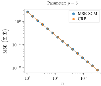
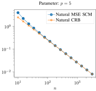
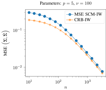
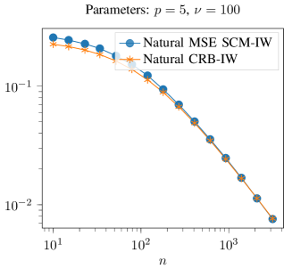
Figures 1(a) and 1(b) show the MSE computed either with the Euclidean distance or the natural distance and the corresponding CRB. We retrieve the classical result in the Euclidean case where the SCM is proven to be efficiency at finite distance. On the opposite, this efficiency at finite distance is lost when we consider the natural properties of a covariance matrix. This result is also known and firstly given in [12].

(a) Euclidean CRB

(b) Natural CRB

Figure 1: Euclidean CRB and MSE (left) and Natural CRB and distance w.r.t. $n$. The data size is $p=5$.

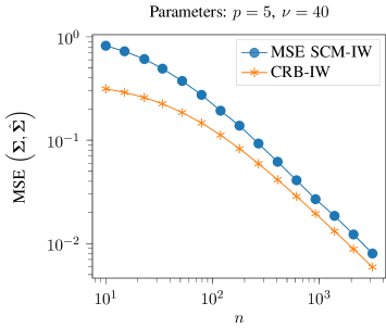
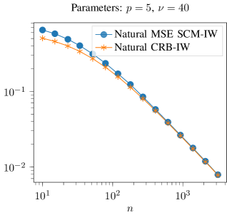
Now, we turn on the study of the MAP estimator and the corresponding CRB. We consider two cases: $\nu=40$ and $\nu=100$. The results are shown in Figures 2(a) and 2(b) for the first value of $\nu$ and in Figures 3(a) and 3(b) for the second one. For both values, conclusions are similar. We have the property of non asymptotic efficiency for the MAP estimator in the Euclidean study. This result was expected since the FIM depended on the studied parameter $\mathbf{\Sigma}$. In the natural study, the asymptotic efficiency seems to be true which was also expected since in this case the FIM is just equal to identity matrix up to a factor. It allows to notice that the MAP estimator is here a very good estimator as soon as we have enough samples to estimate it (obviously depending on $\nu$).

(a) Euclidean CRB

(b) Natural CRB

Figure 2: Bayesian Euclidean CRB and MSE (left) and Bayesian Natural CRB and expectation of the natural distance w.r.t. $n$. The data size is $p=5$ and the number of degrees of freedom of the $\mathcal{IW}$ prior is $\nu=40$.

(a) Euclidean CRB

(b) Natural CRB

Figure 3: Bayesian Euclidean CRB and MSE (left) and Bayesian Natural CRB and expectation of the natural distance w.r.t. $n$. The data size is $p=5$ and the number of degrees of freedom of the $\mathcal{IW}$ prior is $\nu=100$.

VI Conclusion

When the parameter to estimate lies in a manifold and that we assume that it follows a prior distribution, we have proposed a new natural inequality between a covariance of the estimation error defined with geometric tools and an intrinsic CRB. This derivation is made by using some assumptions on the manifold of interest and the prior distribution. We illustrated this result by considering the problem of covariance estimation in particular when the data follow a Gaussian distribution and the prior distribution is an inverse Wishart. Numerical simulation leaded to interesting conclusions on the MAP estimator which seems to be asymptotic efficiency in the natural inequality which is not the case when the study is made with the Euclidean formalism.

Appendix A Extension of results of [26]

$\mathbf{S}\sim\mathcal{W}^{C}_{N}(K,\frac{1}{K}\bm{\Sigma})$ and since $\operatorname{Tr}(\mathbf{A}_{(1)}\ldots\mathbf{A}_{(n)})=\sum_{i_{1},\ldots,i_{n}}a^{(1)}_{i_{1}i_{2}}\ldots a^{(n)}_{i_{n}i_{1}}$:

$$\begin{array}[]{l}E[\operatorname{Tr}(\mathbf{A}\mathbf{S}\mathbf{B}\mathbf{S})\operatorname{Tr}(\mathbf{C}\mathbf{S})]=\operatorname{Tr}(\mathbf{A}\bm{\Sigma}\mathbf{B}\bm{\Sigma})\operatorname{Tr}(\mathbf{C}\bm{\Sigma})\\ +\frac{1}{K}(\operatorname{Tr}(\mathbf{A}\bm{\Sigma}\mathbf{B}\bm{\Sigma}\mathbf{C}\bm{\Sigma})+\operatorname{Tr}(\mathbf{A}\bm{\Sigma}\mathbf{C}\bm{\Sigma}\mathbf{B}\bm{\Sigma})+\operatorname{Tr}(\mathbf{A}\bm{\Sigma})\operatorname{Tr}(\mathbf{B}\bm{\Sigma})\operatorname{Tr}(\mathbf{C}\bm{\Sigma}))\\ +\frac{1}{K^{2}}(\operatorname{Tr}(\mathbf{A}\bm{\Sigma}\mathbf{C}\bm{\Sigma})\operatorname{Tr}(\mathbf{B}\bm{\Sigma})+\operatorname{Tr}(\mathbf{B}\bm{\Sigma}\mathbf{C}\bm{\Sigma})\operatorname{Tr}(\mathbf{A}\bm{\Sigma}))\end{array}$$ (80)

and

$$\begin{array}[]{l}E[\operatorname{Tr}(\mathbf{A}\mathbf{S}\mathbf{B}\mathbf{S})\operatorname{Tr}(\mathbf{C}\mathbf{S}\mathbf{D}\mathbf{S})]=\operatorname{Tr}(\mathbf{A}\bm{\Sigma}\mathbf{B}\bm{\Sigma})\operatorname{Tr}(\mathbf{C}\bm{\Sigma}\mathbf{D}\bm{\Sigma})\\ +\frac{1}{K}(\operatorname{Tr}(\mathbf{A}\bm{\Sigma}\mathbf{B}\bm{\Sigma}\mathbf{C}\bm{\Sigma}\mathbf{D}\bm{\Sigma})+\operatorname{Tr}(\mathbf{A}\bm{\Sigma}\mathbf{C}\bm{\Sigma}\mathbf{D}\bm{\Sigma}\mathbf{B}\bm{\Sigma})+\operatorname{Tr}(\mathbf{A}\bm{\Sigma}\mathbf{B}\bm{\Sigma}\mathbf{D}\bm{\Sigma}\mathbf{C}\bm{\Sigma})\\ +\operatorname{Tr}(\mathbf{A}\bm{\Sigma}\mathbf{D}\bm{\Sigma}\mathbf{C}\bm{\Sigma}\mathbf{B}\bm{\Sigma})+\operatorname{Tr}(\mathbf{A}\bm{\Sigma}\mathbf{B}\bm{\Sigma})\operatorname{Tr}(\mathbf{C}\bm{\Sigma})\operatorname{Tr}(\mathbf{D}\bm{\Sigma})+\operatorname{Tr}(\mathbf{C}\bm{\Sigma}\mathbf{D}\bm{\Sigma})\operatorname{Tr}(\mathbf{A}\bm{\Sigma})\operatorname{Tr}(\mathbf{B}\bm{\Sigma}))\\ \frac{1}{K^{2}}(\operatorname{Tr}(\mathbf{A}\bm{\Sigma}\mathbf{D}\bm{\Sigma}\mathbf{B}\bm{\Sigma})\operatorname{Tr}(\mathbf{C}\bm{\Sigma})+\operatorname{Tr}(\mathbf{A}\bm{\Sigma}\mathbf{C}\bm{\Sigma}\mathbf{B}\bm{\Sigma})\operatorname{Tr}(\mathbf{D}\bm{\Sigma})+\operatorname{Tr}(\mathbf{A}\bm{\Sigma}\mathbf{D}\bm{\Sigma})\operatorname{Tr}(\mathbf{B}\bm{\Sigma}\mathbf{C}\bm{\Sigma})\\ +\operatorname{Tr}(\mathbf{A}\bm{\Sigma}\mathbf{B}\bm{\Sigma}\mathbf{D}\bm{\Sigma})\operatorname{Tr}(\mathbf{C}\bm{\Sigma})+\operatorname{Tr}(\mathbf{A}\bm{\Sigma}\mathbf{B}\bm{\Sigma}\mathbf{C}\bm{\Sigma})\operatorname{Tr}(\mathbf{D}\bm{\Sigma})+\operatorname{Tr}(\mathbf{A}\bm{\Sigma}\mathbf{C}\bm{\Sigma})\operatorname{Tr}(\mathbf{B}\bm{\Sigma}\mathbf{D}\bm{\Sigma})\\ +\operatorname{Tr}(\mathbf{A}\bm{\Sigma})\operatorname{Tr}(\mathbf{B}\bm{\Sigma})\operatorname{Tr}(\mathbf{C}\bm{\Sigma})\operatorname{Tr}(\mathbf{D}\bm{\Sigma})+\operatorname{Tr}(\mathbf{B}\bm{\Sigma}\mathbf{C}\bm{\Sigma}\mathbf{D}\bm{\Sigma})\operatorname{Tr}(\mathbf{A}\bm{\Sigma})+\operatorname{Tr}(\mathbf{A}\bm{\Sigma}\mathbf{C}\bm{\Sigma}\mathbf{D}\bm{\Sigma})\operatorname{Tr}(\mathbf{B}\bm{\Sigma})\\ +\operatorname{Tr}(\mathbf{A}\bm{\Sigma}\mathbf{D}\bm{\Sigma}\mathbf{C}\bm{\Sigma})\operatorname{Tr}(\mathbf{B}\bm{\Sigma})+\operatorname{Tr}(\mathbf{B}\bm{\Sigma}\mathbf{D}\bm{\Sigma}\mathbf{C}\bm{\Sigma})\operatorname{Tr}(\mathbf{A}\bm{\Sigma}))\\ +\frac{1}{K^{3}}(\operatorname{Tr}(\mathbf{A}\bm{\Sigma}\mathbf{D}\bm{\Sigma}\mathbf{B}\bm{\Sigma}\mathbf{C}\bm{\Sigma})+\operatorname{Tr}(\mathbf{A}\bm{\Sigma}\mathbf{C}\bm{\Sigma})\operatorname{Tr}(\mathbf{B}\bm{\Sigma})\operatorname{Tr}(\mathbf{D}\bm{\Sigma})+\operatorname{Tr}(\mathbf{A}\bm{\Sigma}\mathbf{D}\bm{\Sigma})\operatorname{Tr}(\mathbf{B}\bm{\Sigma})\operatorname{Tr}(\mathbf{C}\bm{\Sigma})\\ +\operatorname{Tr}(\mathbf{B}\bm{\Sigma}\mathbf{C}\bm{\Sigma})\operatorname{Tr}(\mathbf{A}\bm{\Sigma})\operatorname{Tr}(\mathbf{D}\bm{\Sigma})+\operatorname{Tr}(\mathbf{B}\bm{\Sigma}\mathbf{D}\bm{\Sigma})\operatorname{Tr}(\mathbf{A}\bm{\Sigma})\operatorname{Tr}(\mathbf{C}\bm{\Sigma})+\operatorname{Tr}(\mathbf{A}\bm{\Sigma}\mathbf{C}\bm{\Sigma}\mathbf{B}\bm{\Sigma}\mathbf{D}\bm{\Sigma}))\end{array}$$ (81)

Appendix B Derivation of $T_{1}$ and $T_{2}$

The proof is described in complex which is more complicated than in real due to the presence of more basis. We recall the expressions of $T_{1}$ and $T_{2}$

$$\begin{array}[]{ccc}T_{1}(i)=\mathbb{E}[\operatorname{Tr}(\bm{\Sigma}^{-1}\bm{\Omega}_{i}\bm{\Sigma}^{-1}\bm{\Sigma}_{0})]&=&\mathbb{E}[\operatorname{Tr}(\mathbf{A}\bm{\Omega}_{i}^{E}\mathbf{A}^{H})]\\ T_{2}(i,j)=\mathbb{E}[\operatorname{Tr}(\bm{\Sigma}^{-1}\bm{\Omega}_{i}\bm{\Sigma}^{-1}\bm{\Sigma}_{0})\operatorname{Tr}(\bm{\Sigma}^{-1}\bm{\Omega}_{j}\bm{\Sigma}^{-1}\bm{\Sigma}_{0})]&=&\mathbb{E}[\operatorname{Tr}(\mathbf{A}\bm{\Omega}_{i}^{E}\mathbf{A}^{H})\operatorname{Tr}(\mathbf{A}\bm{\Omega}_{j}^{E}\mathbf{A}^{H})]\end{array}$$ (82)

where $\mathbf{A}$ is a lower triangular matrix and where all the elements are independent random variables :

$$\begin{array}[]{lll}a_{i,j}&\sim&\mathcal{N_{\mathbb{C}}}(0,1),\,i>j\\ a_{i,i}^{2}&\sim&\frac{1}{2}\chi_{2\left(\nu-i+1\right)}^{2}\end{array}$$ (83)

Instead of using the notations $\bm{\Omega}_{i}^{E}$ and $\bm{\Omega}_{j}^{E}$ for the basis, we come back to the first notation, $\mathbf{\bm{\Omega}}_{ii}^{E}$ and $\mathbf{\bm{\Omega}}_{ij}^{E}$ which is recalled in the following:

• $\mathbf{\bm{\Omega}}_{ii}^{E}$ is an $p$ by $p$ symmetric matrix whose $i$th diagonal element is one, zeros elsewhere

• $\mathbf{\bm{\Omega}}_{ij}^{E}$ is an $p$ by $p$ symmetric matrix whose $ij$th and $ji$th elements are both $2^{-1/2}$, zeros elsewhere. By convention, we use $i>j$.

• $\mathbf{\bm{\Omega}}_{ij}^{h-{E}}$ is an $p$ by $p$ Hermitian matrix whose $ij$th element is $2^{-1/2}\sqrt{-1}$, and $ji$th element is $-2^{-1/2}\sqrt{-1}$, zeros elsewhere ($i>j$).

B-A Calculation of $T_{1}$

We have

$$T_{1}(i)=\mathbb{E}[\operatorname{Tr}(\mathbf{A}\bm{\Omega}_{i}^{E}\mathbf{A}^{H})]=\mathbb{E}[\operatorname{Tr}(\bm{\Omega}_{i}^{E}\mathbf{A}^{H}\bm{\mathbf{A}})]=\operatorname{Tr}(\bm{\Omega}_{i}^{E}\mathbb{E}[\mathbf{A}^{H}\bm{\mathbf{A}}])$$ (84)

First, we are looking for the $\left(i,j\right)-$element of the matrix $\mathbf{A}^{H}\bm{\mathbf{A}}$. The $i^{th}$ row of the matrix $\mathbf{A}^{T}$ is the following vector

$$\left.\mathbf{A}^{H}\right|_{i^{th}\,row}=\left(\underset{i-1\>elements}{\underbrace{\begin{array}[]{ccc}0&\cdots&0\end{array}}}\underset{p-i+1\>elements}{\underbrace{\begin{array}[]{cccc}a_{i,i}^{*}&a_{i+1,i}^{*}&\cdots&a_{p,i}^{*}\end{array}}}\right)$$ (85)

and the $j^{th}$ column of the matrix $\mathbf{A}$ is the following vector

$$\left.\mathbf{A}\right|_{j^{th}\,column}=\left(\underset{j-1\>elements}{\underbrace{\begin{array}[]{ccc}0&\cdots&0\end{array}}}\underset{p-j+1\>elements}{\underbrace{\begin{array}[]{cccc}a_{j,j}&a_{j+1,j}&\cdots&a_{p,j}\end{array}}}\right)^{T}$$ (86)

Then, if $i>j$ the $\left(i,j\right)-$element of the matrix $\mathbf{A}^{H}\bm{\mathbf{A}}$ is given by

$$\left.\mathbf{A}^{H}\bm{\mathbf{A}}\right|_{i,j}=\left.\mathbf{A}^{H}\bm{\mathbf{A}}\right|_{j,i}=a_{i,i}^{*}a_{i,j}+a_{i+1,i}^{*}a_{i+1,j}+\cdots+a_{p,i}^{*}a_{p,j}$$ (87)

and $\mathbb{E}[\left.\mathbf{A}^{H}\bm{\mathbf{A}}\right|_{i,j}]=0$ since all the RV are independent and $\mathbb{E}[a_{i,j}]=0$ for $i\neq j$. Consequently, with the same reasoning when $j>i$ one can conclude that $\mathbb{E}[\mathbf{A}^{H}\bm{\mathbf{A}}]$ is a diagonal matrix. If now $i=j$, then

$$\left.\mathbf{A}^{H}\bm{\mathbf{A}}\right|_{i,i}=\underset{p-i+1\,elements}{\underbrace{a_{i,i}^{2}+\left\|a_{i+1,i}\right\|^{2}+\cdots+\left\|a_{p,i}\right\|^{2}}}$$ (88)

Since $a_{i,i}^{2}\sim\frac{1}{2}\chi_{2\left(\nu-i+1\right)}^{2}$ and $a_{i,j\neq i}\sim\mathcal{N_{\mathbb{C}}}\left(0,1\right)$, and the independence of all the RV, one has $\mathbb{E}\left[a_{i,i}^{2}\right]=\nu-i+1$ (which appears once) and $\mathbb{E}\left[\left\|a_{i,j\neq i}\right\|^{2}\right]=1$ (which appears $p-i$ times) and

$$\mathbb{E}\left[\left.\mathbf{A}^{H}\bm{\mathbf{A}}\right|_{i,i}\right]=\nu-i+1+p-i=\nu+p-2i+1$$ (89)

Now if $\mathbf{\bm{\Omega}}_{i}^{E}:=\mathbf{\bm{\Omega}}_{ii}^{E}$, one obtains $T_{1}=\operatorname{Tr}(\bm{\Omega}_{ii}^{E}\mathbb{E}[\mathbf{A}^{H}\bm{\mathbf{A}}])=\mathbb{E}\left[\left.\mathbf{A}^{H}\bm{\mathbf{A}}\right|_{i,i}\right]=\nu+p-2i+1$ and, if $\mathbf{\bm{\Omega}}_{i}^{E}:=\mathbf{\bm{\Omega}}_{ij}^{E}$, then $\bm{\Omega}_{ij}^{E}\mathbb{E}[\mathbf{A}^{H}\bm{\mathbf{A}}]$ is a matrix with zeros on its diagonal and its trace is then equal to zero. Consequently,

$$T_{1}(i)=\left\{\begin{array}[]{c}0\>if\>\mathbf{\bm{\Omega}}_{i}^{E}:=\mathbf{\bm{\Omega}}_{ij}^{E}\\ \nu+p-2i+1\>if\,\mathbf{\bm{\Omega}}_{i}^{E}:=\mathbf{\bm{\Omega}}_{ii}^{E}\end{array}\right.$$ (90)

B-B Calculation of $T_{2}$

Let’s first analyze the term $\operatorname{Tr}(\bm{\Omega}_{i}^{E}\mathbf{A}^{H}\mathbf{A})$ (since we know from the calculus of $T_{1}$ the structure of $\left.\mathbf{A}^{H}\bm{\mathbf{A}}\right|_{i,j}$). If $\mathbf{\bm{\Omega}}_{i}^{E}:=\mathbf{\bm{\Omega}}_{ii}^{E}$ then

$$\operatorname{Tr}(\bm{\Omega}_{ii}^{E}\mathbf{A}^{H}\mathbf{A})=\left.\mathbf{A}^{H}\bm{\mathbf{A}}\right|_{i,i}=\underset{p-i+1\,elements}{\underbrace{a_{i,i}^{2}+\left\|a_{i+1,i}\right\|^{2}+\cdots+\left\|a_{p,i}\right\|^{2}}}$$ (91)

If $\mathbf{\bm{\Omega}}_{i}^{E}:=\mathbf{\bm{\Omega}}_{ij}^{E}$ then

$$\begin{array}[]{lll}\operatorname{Tr}(\bm{\Omega}_{ij}^{E}\mathbf{A}^{H}\mathbf{A})&=&\frac{1}{\sqrt{2}}\left(a_{i,i}a_{i,j}+a_{i+1,i}^{*}a_{i+1,j}+\cdots\right.\\ &&\left.+a_{p,i}^{*}a_{p,j}+a_{i,i}a_{i,j}^{*}+a_{i+1,i}a_{i+1,j}^{*}+\cdots+a_{p,i}a_{p,j}^{*}\right)\end{array}$$ (92)

where we have $2\left(p-i+1\right)$ elements. If $\mathbf{\bm{\Omega}}_{i}^{E}:=\mathbf{\bm{\Omega}}_{ij}^{h-{E}}$ then

$$\begin{array}[]{lll}\operatorname{Tr}(\bm{\Omega}_{ij}^{h-{E}}\mathbf{A}^{H}\mathbf{A})&=&\frac{\sqrt{-1}}{\sqrt{2}}\left(-a_{i,i}a_{i,j}-a_{i+1,i}^{*}a_{i+1,j}-\cdots\right.\\ &&\left.-a_{p,i}^{*}a_{p,j}+a_{i,i}a_{i,j}^{*}+a_{i+1,i}a_{i+1,j}^{*}+\cdots+a_{p,i}a_{p,j}^{*}\right)\end{array}$$ (93)

Second, let’s study $\operatorname{Tr}(\bm{\Omega}_{i}^{E}\mathbf{A}^{H}\mathbf{A})\operatorname{Tr}(\bm{\Omega}_{j}^{E}\mathbf{A}^{H}\mathbf{A})$ and its expectation (i.e. $T_{2}$). Several cases can appear

Case 1

If $\mathbf{\bm{\Omega}}_{i}^{E}:=\mathbf{\mathsf{\bm{\Omega}}}_{ii}^{E}:=\mathbf{\bm{\Omega}}_{j}^{E}$

$$\begin{array}[]{lll}T_{2}(i,j)&=&\mathbb{E}[\operatorname{Tr}^{2}(\bm{\Omega}_{ii}^{E}\mathbf{A}^{H}\mathbf{A})]\\ &=&\mathbb{E}\left[\left(a_{i,i}^{2}+\left\|a_{i+1,i}\right\|^{2}+\cdots+\left\|a_{p,i}\right\|^{2}\right)^{2}\right]\\ &=&\text{VAR}\left(a_{i,i}^{2}+\left\|a_{i+1,i}\right\|^{2}+\cdots+\left\|a_{p,i}\right\|^{2}\right)+(\mathbb{E}\left[a_{i,i}^{2}+\left\|a_{i+1,i}\right\|^{2}+\cdots+\left\|a_{p,i}\right\|^{2}\right])^{2}\\ &=&\left(\nu-i+1\right)+\left(\nu+p-2i+1\right)^{2}\end{array}$$ (94)

Case 2

If $\mathbf{\bm{\Omega}}_{i}^{E}:=\mathbf{\bm{\Omega}}_{ii}^{E}$ and $\mathbf{\bm{\Omega}}_{j}^{E}:=\mathbf{\bm{\Omega}}_{jj}^{E}$ with $i\neq j$

$$\begin{array}[]{lll}T_{2}(i,j)&=&\mathbb{E}[\operatorname{Tr}(\bm{\Omega}_{ii}^{E}\mathbf{A}^{H}\mathbf{A})\operatorname{Tr}(\bm{\Omega}_{jj}^{E}\mathbf{A}^{H}\mathbf{A})]\\ &=&\mathbb{E}\left[\left(\underset{p-i+1\,elements}{\underbrace{a_{i,i}^{2}+\left\|a_{i+1,i}\right\|^{2}+\cdots+\left\|a_{p,i}\right\|^{2}}}\right)\left(\underset{p-j+1\,elements}{\underbrace{a_{j,j}^{2}+\left\|a_{j+1,j}\right\|^{2}+\cdots+\left\|a_{p,j}\right\|^{2}}}\right)\right]\\ &=&\left(\nu-2i+p+1\right)\left(\nu-2j+p+1\right)\\ \\ \end{array}$$ (95)

Case 3

If $\mathbf{\bm{\Omega}}_{i}^{E}:=\mathbf{\bm{\Omega}}_{ii}^{E}$ and $\mathbf{\bm{\Omega}}_{j}^{E}:=\mathbf{\bm{\Omega}}_{kl}^{E}$ (with $k>l$ but where possibly $k$ or $l$ can be equal to $i$)

$$\begin{array}[]{l}T_{2}(i,j)=\frac{1}{\sqrt{2}}\mathbb{E}\left[\left(a_{i,i}^{2}+\left\|a_{i+1,i}\right\|^{2}+\cdots+\left\|a_{p,i}\right\|^{2}\right)\right.\\ \left.\left(a_{k,k}a_{k,l}+a_{k+1,k}^{*}a_{k+1,l}+\cdots+a_{p,k}^{*}a_{p,l}+a_{k,k}a_{k,l}^{*}+a_{k+1,k}a_{k+1,l}^{*}+\cdots+a_{p,k}a_{p,l}^{*}\right)\right]\end{array}$$ (96)

Each terms is the product of an expectation of up to 3 random variables. More precisely, $T_{2}$ is made with terms that can only be in one of following situations: (i) $\mathbb{E}\left[a_{i,i}^{2}a_{k,k}a_{k,l}\right]=\mathbb{E}\left[a_{i,i}^{2}a_{k,k}\right]\mathbb{E}\left[a_{k,l}\right]=0$ since $k\neq l$ and $\mathbb{E}\left[a_{k,l}\right]=0$ (same thing when we have $\mathbb{E}\left[a_{i,i}^{2}a_{k,k}a_{k,l}^{*}\right]$). (ii) with $N=\left\{1,\ldots,p-k\right\}$, $\mathbb{E}\left[a_{i,i}^{2}a_{k+N,k}^{*}a_{k+N,l}\right]=\mathbb{E}\left[a_{i,i}^{2}\right]\mathbb{E}\left[a_{k+N,k}^{*}\right]\mathbb{E}\left[a_{k+N,l}\right]=0$ since $k\neq l$ and $N>0$ one always has $a_{k+N,k}\neq a_{k+N,l}\neq a_{i,i}$ (same thing when we have $\mathbb{E}\left[a_{i,i}^{2}a_{k+N,k}a_{k+N,l}^{*}\right]$). (iii) with $Q=\left\{1,\ldots,p-k\right\}$, $\mathbb{E}\left[a_{i+Q,i}^{2}a_{k,k}a_{k,l}\right]=0$ because, the random variables $a_{i+Q,i}^{2}$ and $a_{k,l}$ are the same (i.e. not independent) if and only if $k=i+Q$ and $l=i$ which leads to $\mathbb{E}\left[a_{i+Q,i}^{2}a_{k,k}a_{k,l}\right]=\mathbb{E}\left[a_{k,k}\right]\mathbb{E}\left[a_{k,l}^{3}\right]=0$ since $k\neq l$ and $\mathbb{E}\left[a_{k,l}^{3}\right]=0$ (because $a_{k,l}\sim\mathcal{N}\left(0,1\right)$). Otherwise, $a_{i+Q,i}^{2}$ and $a_{k,l}$ are independent, then $\mathbb{E}\left[a_{i+Q,i}^{2}a_{k,k}a_{k,l}\right]=\mathbb{E}\left[a_{k,k}\right]\mathbb{E}\left[a_{i+Q,i}^{2}\right]\mathbb{E}\left[a_{k,l}\right]=0$ since $k\neq l$ and $\mathbb{E}\left[a_{k,l}\right]=0$. (iv) with $N=\left\{1,\ldots,p-k\right\}$ and $Q=\left\{1,\ldots,p-k\right\}$, $\mathbb{E}\left[\left\|a_{i+Q,i}\right\|^{2}a_{k+N,k}^{*}a_{k+N,l}\right]=0$ because $a_{k+N,k}\bot a_{k+N,l}$ since $k>l$ and $N>0$ (same thing when we have $\mathbb{E}\left[\left\|a_{i+Q,i}\right\|^{2}a_{k+N,k}a_{k+N,l}^{*}\right]$). Consequently, for the Case 3, one always has

$$T_{2}(i,j)=0$$ (97)

and, trivially, the case $\mathbf{\bm{\Omega}}_{j}^{E}:=\mathbf{\bm{\Omega}}_{jj}^{E}$ and $\mathbf{\bm{\Omega}}_{i}^{E}:=\mathbf{\bm{\Omega}}_{kl}^{E}$ (with $k>l$ but where possibly $k$ or $l$ can be equal to $j$) leads also to $T_{2}=0$.

Case 4

If $\mathbf{\bm{\Omega}}_{i}^{E}:=\mathbf{\bm{\Omega}}_{mn}^{E}$ (with $m>n$) and $\mathbf{\bm{\Omega}}_{j}^{E}:=\mathbf{\bm{\Omega}}_{kl}^{E}$ (with $k>l$)

$$\begin{array}[]{lll}T_{2}(i,j)&=&\frac{1}{2}\mathbb{E}\left[\left(a_{m,m}a_{m,n}+a_{m+1,n}^{*}a_{m+1,n}+\cdots\right.\right.\\ &&\left.\left.+a_{p,m}^{*}a_{p,n}+a_{m,m}a_{m,n}^{*}+a_{m+1,m}a_{m+1,n}^{*}+\cdots+a_{p,m}a_{p,n}^{*}\right)\right.\\ &&\left.\left(a_{k,k}a_{k,l}+a_{k+1,k}^{*}a_{k+1,l}+\cdots\right.\right.\\ &&\left.\left.+a_{p,k}^{*}a_{p,l}+a_{k,k}a_{k,l}^{*}+a_{k+1,k}a_{k+1,l}^{*}+\cdots+a_{p,k}a_{p,l}^{*}\right)\right]\end{array}$$ (98)

Concerning terms such that $\mathbb{E}[a_{m,m}a_{m,n}a_{k,k}a_{k,l}^{*}]$ (or $\mathbb{E}[a_{m,m}a_{m,n}^{*}a_{k,k}a_{k,l}]$), if $m=k$ and $n=l$, one has $\mathbb{E}[a_{m,m}a_{m,n}a_{k,k}a_{k,l}^{*}]=\mathbb{E}[a_{m,m}^{2}]\mathbb{E}[\left\|a_{m,n}\right\|^{2}]=\nu-m+1$ since $a_{m,m}^{2}\sim\chi_{\nu-m+1}^{2}$ and $\mathbb{E}[\left\|a_{m,n}\right\|^{2}]=1$. Again if $m=k$ and $n=l$ one also have terms such that $\mathbb{E}[a_{m,m}a_{m,n}^{*}a_{k,k}a_{k,l}^{*}]=\mathbb{E}[a_{m,m}a_{m,n}a_{k,k}a_{k,l}]=0$ since $\mathbb{E}[a_{m,n}^{2}]=0$. Otherwise, $\mathbb{E}[a_{m,m}a_{m,n}a_{k,k}a_{k,l}^{*}]=0$ and $\mathbb{E}[a_{m,m}a_{m,n}^{*}a_{k,k}a_{k,l}]=0$ because $a_{m,n}\bot a_{k,l}$ and $\mathbb{E}\left[a_{k,l}\right]=\mathbb{E}\left[a_{m,n}\right]=0$. Concerning terms such that $\mathbb{E}[a_{m,m}a_{m,n}a_{k+N,k}^{*}a_{k+N,l}]$, $\mathbb{E}[a_{m,m}a_{m,n}a_{k+N,k}a_{k+N,l}^{*}]$, $\mathbb{E}[a_{m+Q,m}^{*}a_{m+Q,n}a_{k,k}a_{k,l}]$ and $\mathbb{E}[a_{m+Q,m}a_{m+Q,n}^{*}a_{k,k}a_{k,l}]$, they are always equal to $0$ since $a_{k+N,k}\bot a_{k+N,l}$ and $a_{m+Q,m}\bot a_{m+Q,n}$.

Finally, $\mathbb{E}[a_{m+Q,m}^{*}a_{m+Q,n}a_{k+N,k}a_{k+N,l}^{*}]=\mathbb{E}[a_{m+Q,m}a_{m+Q,n}^{*}a_{k+N,k}^{*}a_{k+N,l}]=\mathbb{E}[\left\|a_{m+Q,m}\right\|^{2}\left\|a_{m+Q,n}\right\|^{2}]=1$ if and only if $m=k$, $n=l$ and $P=N$ (otherwise one always have at least on zero mean random variable independent other the three others, or the fact that $\mathbb{E}[a_{m,n}^{2}]=0$, and these terms are equal to $0$). Consequently for case 4, if $\mathbf{\bm{\Omega}}_{i}^{E}:=\mathbf{\bm{\Omega}}_{mn}^{E}=\mathbf{\bm{\Omega}}_{j}^{E}$

$$T_{2}(i,j)=\left(\nu-m+1+p-m\right)=\left(\nu-2m+p+1\right)$$

and $T_{2}(i,j)=0$ otherwise.

Case 5

If $\mathbf{\bm{\Omega}}_{i}^{E}:=\mathbf{\bm{\Omega}}_{ii}^{E}$ and $\mathbf{\bm{\Omega}}_{j}^{E}:=\mathbf{\bm{\Omega}}_{kl}^{h-{E}}$ (with $k>l$ but where possibly $k$ or $l$ can be equal to $i$)

$$\begin{array}[]{cc}T_{2}(i,j)=\frac{\sqrt{-1}}{\sqrt{2}}\mathbb{E}\left[\left(a_{i,i}^{2}+\left\|a_{i+1,i}\right\|^{2}+\cdots+\left\|a_{p,i}\right\|^{2}\right)\right.\\ \left.\left(-a_{k,k}a_{k,l}-a_{k+1,k}^{*}a_{k+1,l}-\cdots-a_{p,k}^{*}a_{p,l}+a_{k,k}a_{k,l}^{*}+a_{k+1,k}a_{k+1,l}^{*}+\cdots+a_{p,k}a_{p,l}^{*}\right)\right]\end{array}$$ (99)

An analysis, similar to the one provided in case 3, and using the fact that $\forall N=\left\{1,\ldots,p-k\right\}$, $\mathbb{E}\left[a_{k+N,k}^{*}a_{k+N,l}a_{k+N,k}^{*}\right]=\mathbb{E}\left[a_{k+N,k}^{*}a_{k+N,l}a_{k+N,l}\right]=0$ leads to

$$T_{2}(i,j)=0$$ (100)

Of course, the case $\bm{\mathbf{\Omega}}_{j}^{E}:=\mathbf{\bm{\Omega}}_{jj}^{E}$ and $\mathbf{\bm{\Omega}}_{i}^{E}:=\mathbf{\bm{\Omega}}_{kl}^{h-{E}}$ (with $k>l$ but where possibly $k$ or $l$ can be equal to $j$) leads also to $T_{2}(i,j)=0$.

Case 6

If $\mathbf{\bm{\Omega}}_{i}^{E}:=\mathbf{\bm{\Omega}}_{mn}^{E}$ (with $m>n$) and $\mathbf{\bm{\Omega}}_{j}^{E}:=\mathbf{\bm{\Omega}}_{kl}^{h-{E}}$ (with $k>l$)

$$\begin{array}[]{lll}T_{2}(i,j)&=&\frac{\sqrt{-1}}{2}\mathbb{E}\left[\left(a_{m,m}a_{m,n}+a_{m+1,n}^{*}a_{m+1,n}+\cdots\right.\right.\\ &&\left.\left.+a_{p,m}^{*}a_{p,n}+a_{m,m}a_{m,n}^{*}+a_{m+1,m}a_{m+1,n}^{*}+\cdots+a_{p,m}a_{p,n}^{*}\right)\right.\\ &&\left.\left(-a_{k,k}a_{k,l}-a_{k+1,k}^{*}a_{k+1,l}-\cdots\right.\right.\\ &&\left.\left.-a_{p,k}^{*}a_{p,l}+a_{k,k}a_{k,l}^{*}+a_{k+1,k}a_{k+1,l}^{*}+\cdots+a_{p,k}a_{p,l}^{*}\right)\right]\end{array}$$ (101)

Using all the aforementioned arguments, one find after calculus that

$$T_{2}(i,j)=0$$ (102)

Of course, the case $\mathbf{\bm{\Omega}}_{i}^{E}:=\mathbf{\bm{\Omega}}_{mn}^{h-{E}}$ (with $m>n$) and $\mathbf{\bm{\Omega}}_{j}^{E}:=\mathbf{\bm{\Omega}}_{kl}^{E}$ (with $k>l$) leads also to $T_{2}(i,j)=0$.

Case 7

If $\mathbf{\bm{\Omega}}_{i}^{E}:=\mathbf{\bm{\Omega}}_{mn}^{h-{E}}$ (with $m>n$) and $\mathbf{\bm{\Omega}}_{j}^{E}:=\mathbf{\bm{\Omega}}_{kl}^{h-{E}}$ (with $k>l$)

$$\begin{array}[]{lll}T_{2}(i,j)&=&-\frac{1}{2}\mathbb{E}\left[\left(-a_{m,m}a_{m,n}-a_{m+1,m}^{*}a_{m+1,n}-\cdots\right.\right.\\ &&\left.\left.-a_{p,m}^{*}a_{p,n}+a_{m,m}a_{m,n}^{*}+a_{m+1,m}a_{m+1,n}^{*}+\cdots+a_{p,m}a_{p,n}^{*}\right)\right.\\ &&\left.\left(-a_{k,k}a_{k,l}-a_{k+1,k}^{*}a_{k+1,l}-\cdots\right.\right.\\ &&\left.\left.-a_{p,k}^{*}a_{p,l}+a_{k,k}a_{k,l}^{*}+a_{k+1,k}a_{k+1,l}^{*}+\cdots+a_{p,k}a_{p,l}^{*}\right)\right]\end{array}$$ (103)

An analysis, similar to the one provided in case 4, shows that $T_{2}(i,j)\neq 0$ if and only if $m=k$ and $n=l$. In this case, one obtains easily

$$T_{2}(i,j)=\nu-2m+p+1$$ (104)

Final result

Then one can summary the value of $T_{2}(i,j)\neq 0$ as:

• If $\mathbf{\Omega}_{i}^{E}:=\mathbf{\Omega}_{ii}^{E}:=\mathbf{\Omega}_{j}^{E}$ then $T_{2}(i,j)=\left(\nu-i+1\right)+\left(\nu+p-2i+1\right)^{2}$

• If $\mathbf{\Omega}_{i}^{E}:=\mathbf{\Omega}_{ii}^{E}$ and $\mathbf{\Omega}_{j}^{E}:=\mathbf{\Omega}_{jj}^{E}$ with $i\neq j$ then $T_{2}(i,j)=\left(\nu-2i+p+1\right)\left(\nu-2j+p+1\right)$

• If $\mathbf{\Omega}_{i}^{E}:=\mathbf{\Omega}_{mn}^{E}=\mathbf{\Omega}_{j}^{E}$ then $T_{2}(i,j)=\nu-2m+p+1$

• If $\mathbf{\Omega}_{i}^{E}:=\mathbf{\Omega}_{mn}^{h-E}=\mathbf{\Omega}_{j}^{E}$ then $T_{2}(i,j)=\nu-2m+p+1$

References

- [1] C. Radhakrishna Rao, Information and the Accuracy Attainable in the Estimation of Statistical Parameters, pp. 235–247, Springer New York, New York, NY, 1992.
- [2] H. Cramér, Mathematical Methods of Statistics, New York: Princeton University, 1946.
- [3] A. Bhattacharyya, “On some analogues of the amount of information and their use in statistical estimation,” Sankhya: The Indian Journal of Statistics (1933-1960), vol. 8, no. 1, pp. 1–14, 1946.
- [4] E. W. Barankin, “Locally Best Unbiased Estimates,” The Annals of Mathematical Statistics, vol. 20, no. 4, pp. 477 – 501, 1949.
- [5] Koby Todros and Joseph Tabrikian, “General classes of performance lower bounds for parameter estimation—part ii: Bayesian bounds,” IEEE Transactions on Information Theory, vol. 56, no. 10, pp. 5064–5082, 2010.
- [6] Eric Chaumette, Jèrome Galy, Angela Quinlan, and Pascal Larzabal, “A new barankin bound approximation for the prediction of the threshold region performance of maximum likelihood estimators,” IEEE Transactions on Signal Processing, vol. 56, no. 11, pp. 5319–5333, 2008.
- [7] Tirza Routtenberg and Joseph Tabrikian, “Cyclic barankin-type bounds for non-bayesian periodic parameter estimation,” IEEE Transactions on Signal Processing, vol. 62, no. 13, pp. 3321–3336, 2014.
- [8] H.L. Van Trees, Estimation and modulation theory, vol. 1, John Wiley and Sons, 2001.
- [9] H.L. Van Trees and K. L. Bell, Bayesian Bounds for Parameter Estimation and Nonlinear Filtering/Tracking, John Wiley and Sons, 2007.
- [10] Eric Chaumette, Alexandre Renaux, and Mohammed Nabil El Korso, “A class of weiss–weinstein bounds and its relationship with the bobrovsky–mayer-wolf–zakaï bounds,” IEEE Transactions on Information Theory, vol. 63, no. 4, pp. 2226–2240, 2017.
- [11] J.D. Gorman and A.O. Hero, “Lower bounds for parametric estimation with constraints,” IEEE Transactions on Information Theory, vol. 36, no. 6, pp. 1285–1301, 1990.
- [12] Steven T. Smith, “Covariance, subspace, and intrinsic Cramér-Rao bounds,” IEEE Transactions on Signal Processing, vol. 53, no. 5, pp. 1610–1630, 2005.
- [13] Nicolas Boumal, Optimization and estimation on manifolds, Ph.D. thesis, Université catholique de Louvain, feb 2014.
- [14] Harrie Hendriks, “A cramér-rao type lower bound for estimators with values in a manifold,” Journal of Multivariate Analysis, vol. 38, no. 2, pp. 245–261, 1991.
- [15] J. Xavier and V. Barroso, “Intrinsic variance lower bound (ivlb): an extension of the cramer-rao bound to riemannian manifolds,” in Proceedings. (ICASSP ’05). IEEE International Conference on Acoustics, Speech, and Signal Processing, 2005., 2005, vol. 5, pp. v/1033–v/1036 Vol. 5.
- [16] Victor Solo and Gregory S. Chirikjian, “On the cramer-rao bound in riemannian manifolds with application to so(3),” in 2020 59th IEEE Conference on Decision and Control (CDC), 2020, pp. 4117–4122.
- [17] H. W. M. Hendriks, J. H. M. Janssen, and F. H. Ruymgaart, “A cramer-rao type inequality for random variables in euclidean manifolds,” Sankhya: The Indian Journal of Statistics, Series A (1961-2002), vol. 54, no. 3, pp. 387–401, 1992.
- [18] Arnaud Breloy, Guillaume Ginolhac, Alexandre Renaux, and Florent Bouchard, “Intrinsic cramér–rao bounds for scatter and shape matrices estimation in ces distributions,” IEEE Signal Processing Letters, vol. 26, no. 2, pp. 262–266, 2019.
- [19] S. Bonnabel and A. Barrau, “An intrinsic cramér-rao bound on lie groups,” in International Conference on Networked Geometric Science of Information, 2015, pp. 664–672.
- [20] S. Labsir, D. Medina, J. Vilà-Valls, and E. Chaumette, “An intrinsic mcaulay-seidman bound for parameters evolving on matrix lie groups,” in Proceedings of the 56th Asilomar Conference on Signals, Systems and Computers, 2022.
- [21] P.E. Jupp, “A van trees inequality for estimators on manifolds,” Journal of Multivariate Analysis, vol. 101, no. 8, pp. 1814–1825, 2010.
- [22] M. Ashok Kumar and Kumar Vijay Mishra, “Information geometric approach to bayesian lower error bounds,” 2018.
- [23] E. Weinstein and A. J. Weiss, “A general class of lower bounds in parameter estimation,” IEEE Trans. Inform. Theory, vol. 34, pp. 338–342, 1988.
- [24] H. Karcher, “Riemannian center of mass and mollifier smoothing,” Communications on pure and applied mathematics, vol. 30, pp. 509–541, 1977.
- [25] M. Spivak, A Comprehensive Introduction to Differential Geometry, vol. 1,2, Publish or Perish, Inc., 1999.
- [26] D. Maiwald and D. Kraus, “Calculations of moments of complex wishart and inverse whishart distributed matrices,” IEE Proc. Radar Sonar Navig., vol. 147, no. 4, pp. 162–168, August 2000.