Diversified Node Sampling based Hierarchical Transformer Pooling for Graph Representation Learning

Abstract.

Graph pooling methods have been widely used on downsampling graphs, achieving impressive results on multiple graph-level tasks like graph classification and graph generation. An important line called node dropping pooling aims at exploiting learnable scoring functions to drop nodes with comparatively lower significance scores. However, existing node dropping methods suffer from two limitations: (1) for each pooled node, these models struggle to capture long-range dependencies since they mainly take GNNs as the backbones; (2) pooling only the highest-scoring nodes tends to preserve similar nodes, thus discarding the affluent information of low-scoring nodes. To address these issues, we propose a Graph Transformer Pooling method termed GTPool, which introduces Transformer to node dropping pooling to efficiently capture long-range pairwise interactions and meanwhile sample nodes diversely. Specifically, we design a scoring module based on the self-attention mechanism that takes both global context and local context into consideration, measuring the importance of nodes more comprehensively. GTPool further utilizes a diversified sampling method named Roulette Wheel Sampling (RWS) that is able to flexibly preserve nodes across different scoring intervals instead of only higher scoring nodes. In this way, GTPool could effectively obtain long-range information and select more representative nodes. Extensive experiments on 11 benchmark datasets demonstrate the superiority of GTPool over existing popular graph pooling methods.

1. Introduction

Recent years have witnessed an impressive growth in graph representation learning due to its wide application across various domains such as social network (Ma et al., 2021), chemistry (Baek et al., 2021), biology (Gopinath et al., 2020) and recommender systems (Wu et al., 2021). Among numerous techniques for graph representation learning, graph pooling (Ying et al., 2018), a prominent branch aiming to map a set of nodes into a compact form to represent the entire graph, has attracted great attention in the literature.

Existing graph pooling approaches can be roughly divided into two categories (Liu et al., 2022): flat pooling and hierarchical pooling. The former attempts to design pooling operations (e.g. sum-pool or mean-pool) to generate a graph representation in one step. The latter conducts the pooling operation on graphs in a hierarchical manner, which is beneficial to preserving more structural information than flat pooling methods. Due to the merits of hierarchical pooling, it has become the leading architecture for graph pooling.

There are mainly two types of hierarchical pooling methods (Liu et al., 2022), namely node clustering and node dropping. Node clustering pooling considers graph pooling as a node clustering problem, which maps the nodes into a set of clusters by learning a cluster assignment matrix. While node dropping pooling methods mainly focus on learning a scoring function, then utilize the scores to select top-$K$ nodes and drop all other nodes to downsample the graph. Compared with node clustering pooling, node dropping pooling is usually more efficient and scalable, especially on large graphs. Recently, powerful node dropping pooling methods, including SAGPool (Lee et al., 2019), TopKPool (Gao and Ji, 2019) and ASAP (Ranjan et al., 2020), have been developed and achieved good performance in learning the graph representations. These methods share a similar scheme: identifying and sampling important nodes to build the coarsened graphs hierarchically.

Despite effectiveness, we observe that existing node dropping pooling methods share two common weaknesses: overlooking long-range dependencies and inflexible sampling strategy.

Overlooking long-range dependencies. Existing node dropping methods leverage GNN layers as the backbone, which is naturally inefficient in capturing long-range dependencies of the input graph. Though there are several graph pooling methods (Jain et al., 2021; Baek et al., 2021) that introduce the Transformer architecture to obtain long-range information, they obey the flat pooling design, restricting their capacity to learn the hierarchical graph structure. Hence, there still lack methods that could effectively model long-range relationships meanwhile encoding hierarchical graph structures.

Inflexible sampling strategy. Most existing node dropping methods additionally suffer from only pooling the top-$K$ nodes with higher scores and discarding all other lower scoring nodes. As described in (Li et al., 2020), connected nodes may have similar scores, as their node features tend to be similar. Therefore, preserving only $K$ higher scoring nodes may results in throwing away the whole neighborhood of nodes and inclines to highlight similar nodes. To mitigate this issue, except for the importance score, RepPool (Li et al., 2020) extra adopts a representativeness score to help select nodes from different substructures. Nevertheless, as a top-$K$ sampling method, it is still hard to ensure the diversity of the pooled nodes. As a result, existing node dropping pooling methods can only generate suboptimal graph representations as they ignore the diversities of the sampled nodes.

To tackle the above issues, we propose a novel graph pooling method, termed Graph Transformer Pooling (GTPool), which incorporates the Transformer architecture into node dropping pooling to help the pooled nodes capture long-range information, meanwhile we develop a new node sampling method that can diversely select nodes across different scoring segments. Specifically, we first construct a node scoring module based on the attention matrix to evaluate the significance of nodes based on both global and local context. Then, we utilize a plug-and-play and parameter-free sampling module called Roulette Wheel Sampling (RWS) that is capable of diversely sampling nodes from different scoring intervals. With the indices of sampled nodes, the attention matrix can be refined from $n\times n$ to $\lceil\mu n\rceil\times n$, where $n$ is the number of nodes and $\mu$ is the pooling ratio. In this way, each pooled node can efficiently obtain information from all nodes on the original graph. Besides, our GTPool layer can be integrated with GNN layer to learn graph structures in a hierarchical manner.

To investigate the effectiveness of GTPool, we further conduct experiments on 11 popular benchmarks for the graph classification task. Empirical results show that our GTPool consistently outperforms or achieves competitive performance compared with many state-of-the-art pooling methods.

Our main contributions are summarized as follows:

• To our knowledge, this is the first work that introduces Transformer to node dropping pooling. And we further propose a novel graph pooling method called GTPool, which can be combined with GNN layers to perform hierarchical pooling and makes the pooled nodes capable of capturing long-range relationships.

• We design a plug-and-play and parameter-free sampling strategy called Roulette Wheel Sampling (RWS) that can flexibly select representative nodes across all scoring intervals. Moreover, RWS can boost the performance of other top-$K$ selection-based graph pooling methods by directly replacing the sampling strategy.

• Extensive comparisons on 11 datasets with SOTA baseline methods validate the superior performance of our GTPool on the graph classification task.

2. Related Work

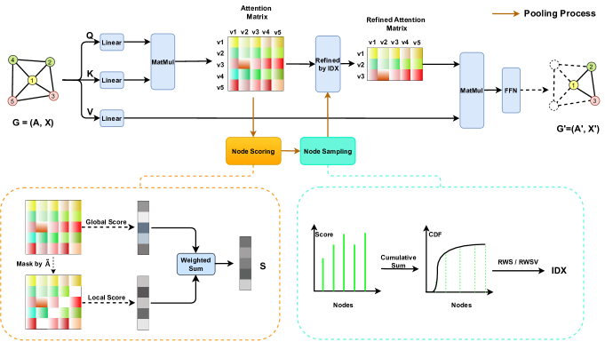
Figure 1. An illustration of the proposed GTPool layer. The scoring module first utilizes the attention matrix to evaluate the significance of nodes from both the local and global views. Then, the sampling module leverages the significance score to diversely select nodes from different sampling intervals. And the attention matrix can be refined with the indices of the sampled nodes. Hence, the pooled nodes can efficiently capture long-range interactions from all other nodes on the original graph. Here we show single head attention and omit the residual connection for better illustration.

In this section, we first review the classical graph neural networks and node dropping pooling methods, then briefly present the most recent emerging works that introduce Transformer to graph pooling.

Graph Neural Networks. Existing graph neural networks (GNNs) can be generally classified into spectral and spatial models. Based on the graph spectral theory, spectral models usually perform convolutional operations in the Fourier domain. Bruna et al. (Bruna et al., 2014) first propose the graph convolutional operation by adopting spectral filters, but it cannot scale to large graphs due to the high-computational cost and non-locality property. To improve the efficiency, Defferrard et al. (Defferrard et al., 2016) utilize an approximation of $K$-polynomial filters that are strictly localized within the radius $K$. Kipf and Welling (Kipf and Welling, 2017) further design a simplified model by leveraging the first-order approximation of the Chebyshev expansion. Different from spectral models, the spatial approaches can directly work on graphs by aggregating information from the local neighbors to update the central node. Among them, GAT (Veličković et al., 2018) employs the attention mechanism in Transformer to distinguish the importance of information from different nodes. As another typical work, GraphSage (Hamilton et al., 2017) provides a general inductive framework that can generate embeddings for unseen nodes by sampling and aggregating features from the local neighborhood of each node. Till now, a variety of GNNs (Klicpera et al., 2019; He et al., 2022; Chen et al., 2020b; Li et al., 2022) have been proposed to handle different kinds of graphs. Nevertheless, these GNNs belong to flat methods that focus on learning node representations for all nodes, but hard to work on the graph classification task directly. Besides, GNNs also suffer from over-smoothing (Chen et al., 2020a) and over-squashing (Alon and Yahav, 2021) problems, causing them unable to efficiently capture long-range pairwise dependencies.

Node Dropping Pooling. Compared to flat pooling, hierarchical pooling takes the hierarchical structures of graphs into consideration, therefore generating more expressive graph representations. With different coarsening manners, hierarchical pooling can be roughly grouped into two categories: node clustering pooling and node dropping pooling. Node clustering pooling (Ying et al., 2018; Bianchi et al., 2020) casts the graph pooling problem into the node clustering problem that map the nodes into a bunch of clusters. As another important line, the key procedure of node dropping pooling (Lee et al., 2019; Gao and Ji, 2019; Ranjan et al., 2020) is to adopt learnable scoring functions to drop nodes with comparatively lower scores. For instance, Gao et al. (Gao and Ji, 2019) propose a simple method named TopKPool that utilizes a learnable vector to calculate the projection scores and uses the scores to select the top ranked nodes. Similarly, as an important variant of TopKPool, SAGPool (Lee et al., 2019) leverages a GNN layer to provide self-attention scores that both consider attributed and topological information and also sample the higher scoring nodes. Different from the above two methods, ASAP (Ranjan et al., 2020) adopts a novel self-attention network along with a modified GNN formulation to capture the importance of each node. Subsequently, multiple types of node dropping pooling methods have emerged by designing more sophisticated scoring functions and more reasonable graph coarsening to select more representative nodes and to retain more important structural information, respectively.

However, based on existing node dropping methods, we find the obtained pooled nodes struggle to capture long-range information, restricting the expressiveness of graph representations. Besides, these methods also suffer from solely sampling higher scoring nodes with similar features, which may results in performing less satisfactory when multiple dissimilar nodes contribute to the graph representations.

Graph Pooling with Transformer. Transformer-based models (Ying et al., 2021; Chen et al., 2022, 2023) have shown impressive performance on various graph mining tasks. Hence, several works have attempted to introduce the Transformer architecture to the graph pooling domain. GraphTrans (Jain et al., 2021) employs a special learnable token to aggregate all pairwise interactions into a single classification vector, which can be actually regarded as a kind of flat pooling. Jinheon et al. (Baek et al., 2021) formulate the graph pooling problem as a multiset encoding problem and propose GMT which is a multi-head attention based global pooling layer. To sum up, there still lacks an effective method that can combine Transformer with graph pooling problem and meanwhile perform hierarchical pooling to obtain more accurate graph representations.

In this paper, we propose GTPool that attempts to introduce Transformer to node dropping pooling methods. GTPool not only can pool graphs in a hierarchical way, but it also samples nodes in a diverse way, enabling it to generate better graph representations.

3. Preliminaries

For preliminaries, we first present the notations and terminologies of attributed graphs for problem formulation, then shortly recap the general descriptions of graph neural networks and the classic Transformer architecture.

Notations. In this paper, we concentrate on the graph classification task, which aims at mapping each of the graphs to a set of labels. We define an arbitrary attributed graph as $\mathcal{G}=(\mathcal{V},\mathcal{E},\mathbf{X})$, where $\mathcal{V}$ and $\mathcal{E}$ are the node set and edge set, respectively. Besides, we have $\mathbf{A}\in\mathbb{R}^{n\times n}$ represents the adjacency matrix, and $\mathbf{X}\in\mathbb{R}^{n\times d}$ represents the feature matrix of $\mathcal{G}$ in which $n$ is the number of nodes and $d$ is the dimension of each feature vector. And $\tilde{\mathbf{A}}=\mathbf{A}+\mathbf{I}_{n}$ denotes the adjacency matrix with self-loops. Considering a graph dataset $\mathcal{D}=\{(\mathcal{G}_{1},y_{1}),(\mathcal{G}_{2},y_{2}),...\}$, the target of the graph classification task is to learn a mapping function $f:\mathcal{G}\to\mathcal{Y}$, where $\mathcal{G}$ is the input graph and $\mathcal{Y}$ is corresponding label.

Graph Neural Networks. In this work, we utilize Graph Convolutional Network (GCN) (Kipf and Welling, 2017) to construct our hierarchical pooling models. It is obvious that our GTPool can also conduct the hierarchical pooling operation based on other GNNs like GIN (Xu et al., 2019) and GAT (Veličković et al., 2018). A standard GCN layer can be formally formulated as:

(1) $$\mathbf{X}^{(l+1)}=\sigma(\tilde{\mathbf{D}}^{-\frac{1}{2}}\tilde{\mathbf{A}}\tilde{\mathbf{D}}^{-\frac{1}{2}}\mathbf{X}^{(l)}\mathbf{W}^{(l)}),$$

where $\sigma$ denotes the non-linear activation, $\tilde{\mathbf{D}}=\sum_{j}\tilde{\mathbf{A}}_{i,j}$ is the degree matrix of $\tilde{\mathbf{A}}$, $\mathbf{W}^{(l)}\in\mathbb{R}^{d\times d}$ a trainable matrix in the $l$-th layer, and $\mathbf{X}^{(l+1)}$ the output of this layer and the initial feature matrix $\mathbf{X}^{(0)}=\mathbf{X}$.

Transformer. The Transformer architecture is comprised of a composition of Transformer layers. Each layer consists of two key components: a multi-head attention module (MHA) and a position-wise feed-forward network (FFN). The MHA module, which stacks several scaled dot-product attention layers, is focused on calculating the similarity between queries and keys. Specifically, let $\mathbf{H}\in\mathbb{R}^{n\times d}$ be the input of the self-attention module where $n$ is the number of input tokens and $d$ is the hidden dimension. The output of the self-attention module can be expressed as:

(2) $$\mathrm{Attention}(\mathbf{Q},\mathbf{K},\mathbf{V})=\mathrm{softmax}\left(\frac{\mathbf{QK}^{\top}}{\sqrt{d_{out}}}\right)\mathbf{V},$$

where $\mathbf{Q}=\mathbf{HW}_{Q},\mathbf{K}=\mathbf{HW}_{K},\mathbf{V}=\mathbf{HW}_{V}$ and $\mathbf{W}_{Q}\in\mathbb{R}^{d\times d},\mathbf{W}_{K}\in\mathbb{R}^{d\times d},\mathbf{W}_{V}\in\mathbb{R}^{d\times d}$ are trainable projection matrices. Besides, $d_{out}$ refers to the dimension of $\mathbf{Q}$.

By concatenating multiple instances of Equation 2, the multi-head attention with $m$ heads can be expressed as:

(3) $$\mathrm{MHA}(\mathbf{H})=\mathrm{Concat}(\mathrm{head}_{1},...,\mathrm{head}_{m})\mathbf{W}_{O},$$

where $\mathrm{head}_{j}=\mathrm{Attention}(\mathbf{Q}_{j},\mathbf{K}_{j},\mathbf{V}_{j})$ and $\mathbf{W}_{O}\in\mathbb{R}^{md\times d}$ is a parameter matrix. $\mathrm{Concat}(\cdot)$ represents the concatenating operation. The output of MHA is then fed into the FFN module that consists of two linear transformations with a ReLU activation in between.

4. Graph Transformer Pooling

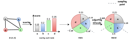
Figure 2. The example describes the sampling process of RWS and RWSV. With pooling ratio $\mu=0.5$, the sampling point is $\{\frac{1}{3},\frac{2}{3}\}$. Obviously, RWS samples node $b$ and $d$, while RWSV samples nodes $b$ and $c$. As a comparison, the top-$K$ selection will sample nodes $c$ and $d$. We can see that RWS and RWSV can sample diversified nodes across different scoring intervals rather than only higher scoring nodes.

In this section, we illustrate our proposed Graph Transformer Pooling (GTPool) in detail. And the architecture is depicted in Figure 1.

4.1. Node Scoring

Similar to existing node dropping methods, a basic step of GTPool is to assign a significance score to each node to measure its importance. Here we combine with the self-attention module  (Vaswani et al., 2017) to score each node from two levels: global context and local context. As the key component of the self-attention module, the attention matrix $\mathcal{A}$ can be calculated by the scaled-dot product of queries ($\mathbf{Q}$) and keys ($\mathbf{K}$):

(4) $$\mathcal{A}=\mathrm{Softmax}\left(\frac{\mathbf{Q}\mathbf{K}^{\top}}{\sqrt{d}}\right),$$

where $\mathbf{Q}\in\mathbb{R}^{n\times d}$, $\mathbf{K}\in\mathbb{R}^{n\times d}$ and $d$ refers to the dimension of $\mathbf{Q}$. Each row of $\mathcal{A}$ indicates the contribution of all input nodes to the target node. Therefore, from the perspective of global context, we compute the global significance score for all nodes as follows:

(5) $$\mathbf{S}_{g}=\sigma(\mathcal{A}\mathbf{V}\mathbf{\Theta}_{g}),$$

where $\sigma$ is an activation function, $\mathbf{V}\in\mathbb{R}^{n\times d}$ is the value matrix and $\mathbf{\Theta}_{g}\in\mathbb{R}^{d\times 1}$ is a learnable vector.

Besides, to measure the importance of local context, we formulate the local significance score as follows:

(6) $$\mathbf{S}_{l}=\sigma(\mathcal{\hat{A}}\mathbf{V}\mathbf{\Theta}_{l}),\\ ~{}~{}\mathbf{\mathcal{\hat{A}}}=\mathcal{A}\odot\mathbf{\tilde{A}},$$

where $\sigma$ is an activation function and $\mathbf{\Theta}_{l}\in\mathbb{R}^{d\times 1}$ is a learnable vector. Here $\mathbf{S}_{l}$ reflects the significance of the local representations of a node’s immediate neighborhood, meanwhile $\mathbf{S}_{g}$ captures the importance of the global representations obtained by each node interacting with all other nodes in the graph.

Altogether, we combine these two scores to measure the importance of different nodes that explicitly take both local and global context into consideration. Specifically, the final scoring vector $\mathbf{S}$ is computed by taking the weighted summation of $\mathbf{S}_{g}$ and $\mathbf{S}_{l}$, which can be written as:

(7) $$\mathbf{S}=\mathrm{Softmax}(\lambda\mathbf{S}_{g}+(1-\lambda)\mathbf{S}_{l}),$$

where $\lambda\in[0,1]$ is a hyperparameter that trades off the global and local scores. For the multi-head attention module, we do summation after calculating the score in each head.

4.2. Node Sampling

Having acquired the final significance score of all nodes, we can select nodes via different sampling strategies. Most existing node dropping methods usually select $K$ highest scoring nodes, which may be redundant and cannot represent the original graph well. Simply performing top-$K$ selection tends to preserve nodes with similar features or topological information, meanwhile low scoring nodes that may be useful for graph representation are recklessly ignored.

To gain a more representative coarsening graph, we attempt to sample nodes in a more diversified way, rather than purely high scoring nodes. Here we perform the pooling operation based on the calculated significance scores. That is to say, the probability of sampling one node is roughly equivalent to its significance score. As described in Equation 7, we apply a $Softmax(\cdot)$ function to normalize $\mathbf{S}$, thus each entry $0\leq\mathbf{S}_{i}\leq 1$ and $\sum_{i=0}^{n}\mathbf{S}_{i}=1$. In this way, these significance scores can be regarded as probabilities. Since the corresponding nodes are discrete variables, the probability mass function can be written as:

(8) $$\mathrm{pmf}({v}_{i})=\begin{cases}\mathbf{S}_{i}\ if\ i\in\{1,2,...,n\},\\ 0\ \ if\ i\notin\{1,2,...,n\},\end{cases}$$

where $v_{i}$ represents the $i$-th node. Based on the above equation, we can further formulate the cumulative distribution function (CDF):

(9) $$\mathrm{CDF}_{i}=\sum_{j=1}^{i}\mathrm{pmf}(v_{j}),~{}~{}i\in\{1,2,...,n\}.$$

Notably, due to the discrete node variable, we cannot directly take the inverse of $\mathrm{CDF}$ to perform inverse transform sampling. To sample nodes via CDF, here we introduce two ways: roulette wheel sampling ($\mathrm{RWS}$) and a variant of roulette wheel sampling ($\mathrm{RWSV}$). Our proposed $\mathrm{RWS}$ adopts a diversified sampling manner similar to roulette wheel selection method. For node $v_{i}$, its cumulative probability interval, which can be seen as the sampling interval, is $[\mathrm{CDF}_{i-1},\mathrm{CDF}_{i}]$. With these $n$ intervals for all nodes, we first generate a random number $k$ from the uniform distribution $U[0,1]$ and see which interval $k$ falls in, then sample the corresponding node. The sampling process can be formulated as:

(10) $$idx_{k}=\mathrm{RWS}(\mathrm{CDF},k),$$

where $idx_{k}$ is the node index selected by $k$. To guarantee the deterministic of training and inference, we leverage a fixed sampling scheme by choosing $k$ as $\{\frac{1}{M+1},\frac{2}{M+1},...,\frac{M}{M+1}\}$, among which $M=\lceil\mu*n\rceil$ is the number of nodes to sample and $\mu$ is the pooling ratio.

By considering the significance score as probability and combining it with a regular sampling scheme, we find $\mathrm{RWS}$ can efficiently preserve low-scoring nodes in most instances. But in practice, low-scoring nodes will be overlooked in some cases, especially when the number of such low-scoring nodes is rare.

To further enhance the preference for low-scoring nodes, we present another sampling method based on $\mathrm{CDF}$ which can be actually interpreted as a variant of $\mathrm{RWS}$. In this approach, with a given $k$, we directly take the index of the node with the nearest cumulative score as the sampling index. Named it as $\mathrm{RWSV}$, the sampling procedure can be shown as:

(11) $$idx_{k}=\mathrm{RWSV}(\mathrm{CDF},k),$$

where $\mathrm{RWSV}(\cdot)$ represents the sampling operation that gets the target node whose cumulative score has a minimum gap with $k$. Same as $\mathrm{RWS}$, here we also leverage the fixed sampling scheme on the value of $k$. As for why $\mathrm{RWSV}$ can be regarded as a variant of $\mathrm{RWS}$, the reason is that $\mathrm{RWSV}$ only slightly adjusts the sampling interval of nodes. As described above, the sampling interval of $v_{i}$ in $\mathrm{RWS}$ is $[\mathrm{CDF}_{i-1},\mathrm{CDF}_{i}]$. While for $\mathrm{RWSV}$, we find the sampling interval for $v_{i}$ is partitioned as:

(12) $${interval}({v}_{i})=\begin{cases}[0,\frac{\mathrm{CDF}_{i}+\mathrm{CDF}_{i+1}}{2}]\ \ if\ \ i=0,\\ [\frac{\mathrm{CDF}_{i-1}+\mathrm{CDF}_{i}}{2},\frac{\mathrm{CDF}_{i}+\mathrm{CDF}_{i+1}}{2}]\ \ if\ \ i\in\{2,...,n-1\},\\ [\frac{\mathrm{CDF}_{i-1}+\mathrm{CDF}_{i}}{2},1]\ \ if\ i=n.\end{cases}$$

Compared with $\mathrm{RWS}$, the sampling intervals for low-scoring nodes are clearly enlarged. Thus $\mathrm{RWSV}$ has the ability to preserve more low-scoring nodes. Figure 2 provides an example about the sampling process of RWS and RWSV. Practically, we find that $\mathrm{RWSV}$ outperforms $\mathrm{RWS}$ on most chosen benchmarks, which also verifies the effectiveness of the adjusted sampling intervals.

During the sampling process, another problem is that a node may be sampled more than once. Therefore, we concretely provide a re-sampling strategy to ensure the uniqueness of the pooled nodes. The basic re-sampling rule is that for both $\mathrm{RWS}$ and $\mathrm{RWSV}$, if the target node has been selected before, we utilize the nearest left neighboring node on the roulette wheel for replacement. After the sampling and re-sampling operation, we can obtain $M$ unique nodes, and their indices can be expressed as $\mathbf{idx}=\{idx_{1},idx_{2},...,idx_{M}\}$.

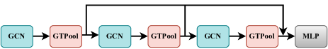
Figure 3. The hierarchical pooling architecture of GTPool. Following the design of previous works, the architecture is constructed by three GCN layers and each layer is followed with a GTPool layer.

4.3. Graph Transformer Pooling

Based on the proposed node scoring and node sampling method, we continue to introduce the pooling process within the Transformer pooling layer to get a coarsened graph $\mathcal{G}^{{}^{\prime}}=(\mathbf{A}^{{}^{\prime}},\mathbf{X}^{{}^{\prime}})$.

Update the Adjacency Matrix. With the indices of the pooled nodes, we can update its adjacency matrix by selecting the corresponding rows and columns. The new adjacency matrix $\mathbf{{A}}^{{}^{\prime}}$ can be expressed as:

(13) $$\mathbf{{A}}^{{}^{\prime}}=\mathbf{{A}}_{\mathbf{idx},\mathbf{idx}},$$

where $\mathbf{{A}}^{{}^{\prime}}\in\mathbb{R}^{M\times M}$.

Update the Attribute Matrix. Here, we first utilize the obtained indices to generate a refined attention matrix by preserving the rows of the corresponding indices, which can be formulated as:

(14) $$\mathcal{A}^{{}^{\prime}}=\mathcal{A}_{\mathbf{idx},:},$$

where $\mathcal{A}^{{}^{\prime}}\in\mathbb{R}^{M\times n}$ denotes the refined attention matrix. Then, to acquire $M$ pooled nodes, we leverage $\mathcal{A}^{{}^{\prime}}$ to replace the original attention matrix $\mathcal{A}$ such that:

(15) $$\mathbf{\hat{X}}=\mathcal{A}^{{}^{\prime}}\mathbf{V}+\mathbf{X}_{\mathbf{idx},:},$$

where $\mathbf{\hat{X}},\mathbf{X}_{\mathbf{idx},:}\in\mathbb{R}^{M\times d}$ and $\mathbf{X}_{\mathbf{idx},:}$ is the residual bias term that denotes the original attribute of the pooled nodes. Notably, by Equation 15, each sampled node can sincerely react with all other nodes on the original graph, thus effectively capturing long-range dependencies. After that, the output $\mathbf{\hat{X}}$ is fed into a standard FFN module in the Transformer layer which consists of two linear layers and a GeLU activation. The process can be formally described as:

(16) $$\mathbf{X}^{{}^{\prime}}=\mathrm{FFN}(\mathrm{LN}(\mathbf{\hat{X}}))+\mathbf{\hat{X}},$$

where $\mathrm{LN}(\cdot)$ indicates layer normalization and $\mathbf{X}^{{}^{\prime}}\in\mathbb{R}^{M\times d}$ is the final output embeddings of the sampled nodes.

In conclusion, with the two updating steps above, we can explicitly generate a new refined graph $\mathcal{G}^{{}^{\prime}}=(\mathbf{A}^{{}^{\prime}},\mathbf{X}^{{}^{\prime}})$.

4.4. Model Architecture

In this subsection, we concretely present the pooling architecture that we utilize in this paper for graph classification. Based on the proposed sampling method RWS and its variant RWSV, we name our pooling operators as GTPool and GTPool-V, respectively. Here, we take GTPool as the example.

As shown in Figure 3, following the setting of previous works (Lee et al., 2019; Baek et al., 2021; Bianchi et al., 2020), there are three blocks in the architecture, each of which consists of a graph convolutional layer and a GTPool layer. For the graph-level representation, we first readout the output of each GTPool layer, and then get their summation, which can be formulated as:

(17) $$\mathbf{h}_{g}=\sum_{i=1}^{l}Readout(GTPool_{i}(GCN_{i}(\mathbf{X}_{i},\mathbf{A}_{i})),$$

where $\mathbf{h}_{g}$ is the graph representation, $l$ is 3 in Figure 3, $\mathbf{X}_{i}$ and $\mathbf{A}_{i}$ are the input feature matrix and adjacency matrix to the $i$-th layer, respectively.

With this hierarchical architecture, we can obtain more expressive graph representations than existing node dropping methods due to the following merits: (1) the RWS (or RWSV) can preserve diverse representative nodes rather than $k$ higher scoring nodes with similar attributes; (2) the pooled nodes have captured both local and global information while existing methods only aggregate local information.

5. Experiments

Table 1. Test performance on 11 benchmarks from TUDatasets and OGB. The shown results are mean ($\%$) and deviation ($\%$) over 10 different runs. The best results appear in bold and hyphen (-) indicates out-of-resources that take more than 10 days.

Model	MUTAG $\uparrow$	ENZYMES $\uparrow$	PROTEINS $\uparrow$	PTC-MR $\uparrow$	Synthie $\uparrow$	IMDB-B $\uparrow$	IMDB-M $\uparrow$	HIV $\uparrow$	TOX21 $\uparrow$	TOXCAST $\uparrow$	BBBP $\uparrow$
GCN	69.50 $\pm$ 1.78	43.52 $\pm$ 1.12	73.24 $\pm$ 0.73	55.72 $\pm$ 1.64	58.61 $\pm$ 1.62	73.26 $\pm$ 0.46	50.39 $\pm$ 0.41	76.81 $\pm$ 1.01	75.04 $\pm$ 0.80	60.63 $\pm$ 0.51	65.47 $\pm$ 1.83
GIN	81.39 $\pm$ 1.53	40.19 $\pm$ 0.84	71.46 $\pm$ 1.66	56.39 $\pm$ 1.25	59.20 $\pm$ 0.73	72.78 $\pm$ 0.86	48.13 $\pm$ 1.36	75.95 $\pm$ 1.35	73.27 $\pm$ 0.84	60.83 $\pm$ 0.46	67.65 $\pm$ 3.00
Set2Set	69.89 $\pm$ 1.94	42.92 $\pm$ 2.05	73.27 $\pm$ 0.85	54.52 $\pm$ 1.69	46.12 $\pm$ 2.71	73.10 $\pm$ 0.48	50.15 $\pm$ 0.58	73.42 $\pm$ 2.34	73.42 $\pm$ 0.67	59.76 $\pm$ 0.65	64.43 $\pm$ 2.16
SortPool	71.94 $\pm$ 3.55	36.17 $\pm$ 2.58	73.17 $\pm$ 0.88	52.62 $\pm$ 2.11	50.18 $\pm$ 1.77	72.12 $\pm$ 1.12	48.18 $\pm$ 0.63	71.82 $\pm$ 1.63	69.54 $\pm$ 0.75	58.69 $\pm$ 1.71	65.98 $\pm$ 1.70
DiffPool	79.22 $\pm$ 1.02	51.27 $\pm$ 2.89	73.03 $\pm$ 1.00	55.26 $\pm$ 3.84	62.75 $\pm$ 0.74	73.14 $\pm$ 0.70	51.31 $\pm$ 0.72	75.64 $\pm$ 1.86	74.88 $\pm$ 0.81	62.28 $\pm$ 0.56	68.25 $\pm$ 0.96
$\mathrm{SAGPool}_{g}$	76.78 $\pm$ 2.12	36.30 $\pm$ 2.51	72.02 $\pm$ 1.08	54.38 $\pm$ 1.96	51.17 $\pm$ 1.71	72.16 $\pm$ 0.88	49.47 $\pm$ 0.56	74.56 $\pm$ 1.69	71.10 $\pm$ 1.06	59.88 $\pm$ 0.79	65.16 $\pm$ 1.93
$\mathrm{SAGPool}_{h}$	73.67 $\pm$ 4.28	34.12 $\pm$ 1.75	71.56 $\pm$ 1.49	53.82 $\pm$ 2.44	51.75 $\pm$ 0.66	72.55 $\pm$ 1.28	50.23 $\pm$ 0.44	71.44 $\pm$ 1.67	69.81 $\pm$ 1.75	58.91 $\pm$ 0.80	63.94 $\pm$ 2.59
TopKPool	67.61 $\pm$ 3.36	29.77 $\pm$ 2.74	70.48 $\pm$ 1.01	55.59 $\pm$ 2.43	50.64 $\pm$ 0.47	71.74 $\pm$ 0.95	48.59 $\pm$ 0.72	72.27 $\pm$ 0.91	69.39 $\pm$ 2.02	58.42 $\pm$ 0.91	65.19 $\pm$ 2.30
MincutPool	79.17 $\pm$ 1.64	25.33 $\pm$ 1.47	74.72 $\pm$ 0.48	54.68 $\pm$ 2.45	52.61 $\pm$ 1.44	72.65 $\pm$ 0.75	51.04 $\pm$ 0.70	75.37 $\pm$ 2.05	75.11 $\pm$ 0.69	62.48 $\pm$ 1.33	65.97 $\pm$ 1.13
StructPool	79.50 $\pm$ 1.75	55.60 $\pm$ 1.94	75.16 $\pm$ 0.86	55.72 $\pm$ 1.41	55.67 $\pm$ 0.92	72.06 $\pm$ 0.64	50.23 $\pm$ 0.53	75.85 $\pm$ 1.81	75.43 $\pm$ 0.79	62.17 $\pm$ 0.61	67.01 $\pm$ 2.65
ASAP	77.83 $\pm$ 1.49	20.10 $\pm$ 1.13	73.92 $\pm$ 0.63	55.68 $\pm$ 1.45	47.93 $\pm$ 1.36	72.81 $\pm$ 0.50	50.78 $\pm$ 0.75	72.86 $\pm$ 1.40	72.24 $\pm$ 1.66	58.09 $\pm$ 1.62	63.50 $\pm$ 2.47
HaarPool	66.11 $\pm$ 1.50	-	-	-	-	73.29 $\pm$ 0.34	49.98 $\pm$ 0.57	-	-	-	66.11 $\pm$ 0.82
GMT	83.44 $\pm$ 1.33	37.38 $\pm$ 1.52	75.09 $\pm$ 0.59	55.41 $\pm$ 1.30	52.65 $\pm$ 0.09	73.48 $\pm$ 0.76	50.66 $\pm$ 0.82	77.56 $\pm$ 1.25	77.30 $\pm$ 0.59	65.44 $\pm$ 0.58	68.31 $\pm$ 1.62
GTPool	87.64 $\pm$ 0.34	61.09 $\pm$ 0.85	75.42 $\pm$ 0.09	61.17 $\pm$ 0.18	67.50 $\pm$ 0.61	74.04 $\pm$ 0.33	50.89 $\pm$ 0.22	77.94 $\pm$ 0.46	77.32 $\pm$ 0.12	65.34 $\pm$ 0.87	70.15 $\pm$ 0.29
GTPool-V	88.15 $\pm$ 0.45	61.31 $\pm$ 0.81	75.68 $\pm$ 0.06	60.91 $\pm$ 0.09	68.08 $\pm$ 0.75	74.23 $\pm$ 0.44	51.49 $\pm$ 0.18	78.36 $\pm$ 0.35	77.45 $\pm$ 0.56	65.18 $\pm$ 1.12	70.68 $\pm$ 0.33

In this section, we evaluate our proposed methods: GTPool (with RWS) and GTPool-V (with RWSV) on several graph benchmarks for graph classification. Various strong baselines from the field of graph pooling are elaborately selected to compare with our methods. To further identify the factors that drive the performance, we conduct ablation studies to analyze the contribution of each key component in our GTPool.

5.1. Experimental Setup

We first briefly introduce the datasets, baselines, and basic configurations used in our experiments.

Datasets. We conduct experiments on 11 widely used datasets to validate the effectiveness of our model. Specifically, we adopt seven datasets from TUDatasets (Morris et al., 2020), including MUTAG, ENZYMES, PROTEINS, PTC-MR, Synthie, IMDB-B and IMDB-M with accuracy for evaluation metric. Besides, we employ four molecule datasets from Open Graph Benchmark (Hu et al., 2020), including HIV, Tox21, ToxCast and BBBP with ROC-AUC for evaluation metric. The detailed statistics are summarized in Appendix A.1.

Baselines. We first consider two popular backbones for comparison: GCN (Kipf and Welling, 2017) and GIN (Xu et al., 2019). Then, we utilize four node dropping methods that drop nodes with lower scores, including SortPool (Zhang et al., 2018), SAGPool (Lee et al., 2019), TopKPool (Gao and Ji, 2019) and ASAP (Ranjan et al., 2020). As another mainstream graph pooling method, we also select four node clustering models that group a set of nodes into a cluster, including DiffPool (Ying et al., 2018), MinCutPool (Bianchi et al., 2020), HaarPool (Wang et al., 2019) and StructPool (Yuan and Ji, 2020). Besides, we additionally choose two commonly used baselines: Set2Set (Vinyals et al., 2016) and GMT (Baek et al., 2021). Set2Set utilizes a recurrent neural network to encode all nodes with content-based attention. GMT formulates graph pooling as a multiset encoding problem and can be actually regarded as a combination of node clustering method with Transformer.

Configurations. For the chosen benchmarks from TUDatasets, we follow the dataset split in (Zhang et al., 2018; Xu et al., 2019; Baek et al., 2021) and conduct 10-fold cross-validation to evaluate the model performance. The initial node attribute we use is in line with the fair comparison setup in (Errica et al., 2020). For datasets from OGB, we follow the original feature extraction and the provided standard dataset splitting in (Hu et al., 2020). More experimental and hyperparameter details are described in Appendix B.

5.2. Performance Comparison

We compare the performance of our proposed GTPool and GTPool-V with the baseline methods on 11 benchmark datasets for the graph classification task.

For the seven benchmarks from TUDatasets, we report the average accuracy with standard deviation after running 10-fold cross-validation ten different times. The experimental results are summarized in Table 1, and the best results appear in bold. First, it is evident that both GTPool and GTPool-V obtain better or competitive performance as compared to these popular pooling methods. To be specific, our proposed methods achieve approximate $4.71\%,5.71\%,4.78\%,5.32\%$ higher accuracy over the best baselines on MUTAG, ENZYMES, PTC-MR and Synthie datasets respectively, demonstrating the effectiveness and superiority of our methods. Next, one can see that the proposed models consistently outperform DiffPool and MincutPool on all the datasets, which reveals the importance of combining local context and global context. Compared with SAGPool, TopKPool, and ASAP, the improved performance can be attributed to the better capacity of our methods to preserve more representative nodes. Especially, the performance of our methods significantly surpasses GMT, indicating that hierarchical pooling brings more improvement than global pooling when cooperating with Transformer. Besides, we can also observe that GMT, GTPool and GTPool-V gain better performance than other graph pooling counterparts, showing the necessity of introducing Transformer to the graph pooling domain.

To validate the effectiveness of our proposed method on diverse datasets, we further conduct experiments on four molecule datasets from the Open Graph Benchmark. By running each experiment 10 times and taking the average and standard deviation of the corresponding metric, the obtained experimental results are reported in Table 1. Overall, our proposed GTPool and GTPool-V achieve higher performance than other baseline models. It is worth emphasizing that when compared to other node dropping pooling methods and GMT, which is a Transformer-based global pooling method, the superior performance of our GTPool steadfastly confirms the effectiveness of combining Transformer with node dropping pooling to hierarchically learn graph representations.

5.3. Effectiveness of RWS & RWSV

Due to the plug-and-play property of our novel sampling schemes (RWS and RWSV), we further conduct extensive experiments to verify the efficacy by applying them to three typical node dropping methods, including $\mathrm{SAGPool}_{h}$, TopKPool and ASAP. We choose PROTEINS, IMDB-BINARY and BBBP as the benchmarks, and the experimental results are shown in Table 2.

By simply replacing the top-$K$ module with our RWS or RWSV, we can observe that these three modified models achieve significant enhancement on the selected datasets. Specifically, the average improvements across the selected datasets over three node dropping pooling methods are approximately $1.73\%$ on $\mathrm{SAGPool}_{h}$, $1.41\%$ on TopKPool and $0.84\%$ on ASAP. These improvements strongly demonstrate that both RWS and RWSV are more capable of preserving representative nodes than the simply top-$K$ selection. In addition, we can also see that RWSV gains better performance in most cases apart from ASAP on PROTEINS and IMDB-BINARY. Note that RWSV still obtains competitive performance on these two datasets. The empirical results clearly show the importance of adjusting the sampling intervals.

Table 2. Test performance on PROTEINS, IMDB-BINARY and BBBP when applying RWS and RWSV to SAGPool_h, TopKPool and ASAP. The shown results are mean ($\%$) and deviation ($\%$) over 10 different runs. The best results appear in bold.

Model	Method	PROTEINS	IMDB-B	BBBP
$\mathrm{SAGPool}_{h}$	top-$K$	71.56 $\pm$ 1.49	72.55 $\pm$ 1.28	63.94 $\pm$ 2.59
$\mathrm{SAGPool}_{h}$	RWS	72.07 $\pm$ 2.46	73.01 $\pm$ 0.69	65.76 $\pm$ 0.52
$\mathrm{SAGPool}_{h}$	RWSV	73.51 $\pm$ 1.06	73.22 $\pm$ 0.36	66.51 $\pm$ 1.29
TopKPool	top-$K$	70.48 $\pm$ 1.01	71.74 $\pm$ 0.95	65.19 $\pm$ 2.30
TopKPool	RWS	71.42 $\pm$ 1.55	72.66 $\pm$ 0.81	65.40 $\pm$ 0.87
TopKPool	RWSV	72.04 $\pm$ 1.44	73.35 $\pm$ 0.67	66.24 $\pm$ 1.75
ASAP	top-$K$	73.92 $\pm$ 0.63	72.81 $\pm$ 0.50	63.50 $\pm$ 2.47
ASAP	RWS	74.17 $\pm$ 1.12	73.79 $\pm$ 0.71	64.22 $\pm$ 1.65
ASAP	RWSV	74.06 $\pm$ 0.68	73.60 $\pm$ 0.70	64.78 $\pm$ 1.04

5.4. Ablation Studies

Table 3. Ablation studies of GTPool-V on the PROTEINS, IMDB-BINARY and BBBP datasets for graph classification. The best results appear in bold.

Model	PROTEINS	IMDB-B	BBBP
GTPool-V	75.68 $\pm$ 0.06	74.23 $\pm$ 0.44	70.68 $\pm$ 0.33
w/o local significance score	73.03 $\pm$ 0.70	73.38 $\pm$ 0.28	69.47 $\pm$ 0.56
w/o global significance score	75.40 $\pm$ 0.27	73.58 $\pm$ 0.29	70.33 $\pm$ 0.44
top-$K$ selection	73.70 $\pm$ 1.44	73.20 $\pm$ 0.42	67.15 $\pm$ 0.69

In this subsection, we perform a series of ablation studies to verify the key component that drives high performance in our proposed GTPool-V. The ablation results are reported in Table 3.

Significance Score. In order to investigate the effectiveness of the global and local significance scores, we compare our proposed GTPool-V to its variants without global and local significance score modules, respectively. The experimental results show that reasonably incorporating both global and local significance scores can significantly improve the performance of GTPool-V, proving the necessity of considering both. Apparently, one can observe that the performance degradation without the global significance score is more severe than without the local score. In some way, this phenomenon signifies the importance of the local context outweighs the global context.

Roulette Wheel Sampling. To explore whether RWSV brings distinctive enhancement, we conduct a comparative experiment between the proposed RWSV and the most commonly used top-$K$ selection. As described before, top-$K$ selection only samples the higher scoring nodes, discarding all lower scoring nodes. From Table 3, we can observe that RWSV outperforms top-$K$ selection by a large margin, showing the superiority of sampling nodes in an adaptive way.

5.5. Parameter Analysis

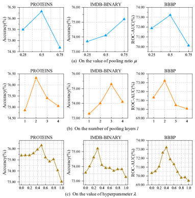
Figure 4. Parameter studies on the pooling ratio $\mu$, the number of pooling layers $l$ and the weight $\lambda$.

We further conduct a variety of studies to investigate the sensitivity of our proposed GTPool-V on three key parameters: the pooling ratio $\mu$, the number of pooling layers $l$ and the weight $\lambda$ that decides which score matters more. The empirical results on PROTEINS, IMDB-BINARY and BBBP by setting different values are illustrated as follows.

On the value of Pooling Ratio $\mu$. Since the value of pooling ratio $\mu$ is closely related to the performance on different datasets, we first test the effect on the value of pooling ratio $\mu$ selecting from $\{0.25,0.5,0.75\}$ and report the performance of GTPool-V. The results are shown in Figure 4 (a). Notably, we can observe that GTPool-V achieves better performance on both PROTEINS and BBBP when setting $\mu$ as $0.5$, and the performance severely drops about $2\%-3\%$ when $\mu=0.75$. The reason can be attributed to the fact that preserving too many nodes will inevitably introduce additional redundancies. Besides, with the increment of $\mu$, the performance on IMDB-BINARY continues to rise because the average number of nodes is lower than PROTEINS and BBBP. Thus, a larger $\mu$ brings more affluent information.

On the number of pooling layers $l$. We further conduct experiments to explore the performance of GTPool with different pooling times. With all other parameters fixed, we vary the number of pooling layers $l$ from $1$ to $4$ and report the results, as shown in Figure 4 (b). In general, the performance curves on three datasets present a moderate increase trend at first, then start to decline. The results demonstrate that it is essential to pick up a suitable pooling time, since stacking too many Transformer-based GTPool-V layers may easily lead to over-fitting.

On the value of weight $\lambda$. A larger $\lambda$ signifies concentrating more on the global context and paying less attention to the local context. To find out how $\lambda$ actually influences the model performance, we conduct a series of studies by varying $\lambda$ from $0$ to $1$ with a step length as 0.1. The experimental results are shown in Figure 4 (c). We interpret the results from two perspectives. First, considering global context can practically bring performance gain for all three datasets. This verifies the effectiveness of the global significance score. Second, with the increment of $\lambda$, the performance on three datasets increases first and then starts to degrade. All in all, these datasets achieve the best performance when $\lambda$ is from 0.3 to 0.5, which demonstrates that properly considering the global context is beneficial for the model performance.

5.6. Computational Efficiency

Table 4. Speedup of GTPool-V. For GTPool-V models trained on PROTEINS, IMDB-BINARY and BBBP, we find that the combination with Transformer increases minimal overhead. Speedup refers to the training iteration speed comparing with SAGPool and a larger number signifies a faster training speed.

Dataset	Model	Forward time (ms)	Backward time (ms)	Speedup
	$\mathrm{SAGPool}_{h}$	26.62 $\pm$ 2.25	31.82 $\pm$ 3.02	1 $\times$
	TopKPool	21.84 $\pm$ 1.60	24.81 $\pm$ 1.72	1.25 $\times$
PROTEINS	ASAP	188.65 $\pm$ 4.75	114.71 $\pm$ 5.12	0.19 $\times$
	GMT	105.46 $\pm$ 6.52	126.44 $\pm$ 5.35	0.25 $\times$
	GTPool-V	24.11 $\pm$ 3.22	20.54 $\pm$ 2.80	1.31 $\times$
	$\mathrm{SAGPool}_{h}$	20.85 $\pm$ 3.73	20.95 $\pm$ 1.44	1 $\times$
	TopKPool	26.32 $\pm$ 2.07	25.84 $\pm$ 1.65	0.80 $\times$
IMDB-B	ASAP	152.18 $\pm$ 5.37	68.08 $\pm$ 3.40	0.19 $\times$
	GMT	66.32 $\pm$ 3.31	82.61 $\pm$ 3.77	0.28 $\times$
	GTPool-V	28.37 $\pm$ 1.95	16.56 $\pm$ 4.11	0.93 $\times$
	$\mathrm{SAGPool}_{h}$	13.94 $\pm$ 4.12	16.86 $\pm$ 3.09	1 $\times$
	TopKPool	9.66 $\pm$ 3.12	14.36 $\pm$ 2.48	1.28 $\times$
BBBP	ASAP	130.78 $\pm$ 6.43	78.22 $\pm$ 4.55	0.15 $\times$
	GMT	43.71 $\pm$ 2.44	158.24 $\pm$ 5.89	0.15 $\times$
	GTPool-V	23.84 $\pm$ 3.58	14.98 $\pm$ 2.78	0.79 $\times$

To quantitatively evaluate the overhead that our GTPool-V brings over typically hierarchical node dropping pooling methods, We report the forward pass time and backward pass time per iteration. The statistical results are shown in Table 4. In order to ensure the fairness of the comparison, we first normalize these models to have approximately similar parameter numbers. Evidently, we can observe that GTPool-V is actually slightly faster to train on the PROTEINS dataset than $\mathrm{SAGPool}_{h}$ and TopKPool, meanwhile exceeding ASAP and GMT by a large margin. For the IMDB-BINARY and BBBP datasets, the training time of GTPool-V is $7-21\%$ slower than $\mathrm{SAGPool}_{h}$ and greatly surpasses ASAP and GMT with more than $64\%$.

5.7. Scalability

Table 5. Scalability of GTPool-V to large graphs. We profile our GTPool-V on these randomly generated graphs and report the runtime in milliseconds.

		Edge Density
Node Count	Model	20%	40%	60%	80%
500	$\mathrm{SAGPool}_{h}$	19.63	23.29	28.50	34.50
	ASAP	217.51	249.49	OOM	OOM
	GMT	25.27	29.02	34.12	37.66
	GTPool-V	30.31	31.74	33.22	34.21
1000	$\mathrm{SAGPool}_{h}$	34.49	53.48	73.26	92.76
	ASAP	OOM	OOM	OOM	OOM
	GMT	42.30	63.72	90.87	115.31
	GTPool-V	41.92	47.07	52.16	57.08
1200	$\mathrm{SAGPool}_{h}$	48.23	71.54	OOM	OOM
	ASAP	OOM	OOM	OOM	OOM
	GMT	49.47	86.18	124.05	OOM
	GTPool-V	48.03	57.10	63.57	OOM

To investigate whether our GTPool-V can scale to large graphs over 100 nodes, we report the runtime of our model on different microbenchmarks with varying node counts and edge densities. These microbenchmarks are comprised of randomly generated Erdos-Renyi graphs with a varying number of nodes from $\{500,1000,1200\}$ and edge density from $\{20\%,40\%,60\%,80\%\}$. We elaborately choose $\mathrm{SAGPool}_{h}$, ASAP and GMT as baselines and the summarized results are shown in Table 5. We can observe that as the number of nodes and edge density increase, our GTPool-V can scale to larger graphs with less runtime. Notably, both $\mathrm{SAGPool}_{h}$ and ASAP meet out of memory errors (OOM) when the number of nodes is 1200 and edge density is $80\%$, but GTPool-V can effectively handle these graphs within roughly a half runtime than GMT.

6. Conclusion

In this paper, we proposed GTPool, a hierarchical and Transformer-based node dropping pooling method for graph structured data. Our method has the following features: hierarchical pooling, consideration of both local and global context, adaptive sampling and be able to capture long-range dependencies for each pooled node. A GTPool layer is actually constructed based on a Transformer encoder layer combining with a scoring module and a sampling module. Specifically, GTPool first leverages the global and local context to score each node, then uses an adaptive roulette wheel sampling (RWS) module to diversely select nodes rather than samping only $M$ higher scoring nodes. With the indices of the sampled nodes, we can refine the attention matrix from $n\times n$ to $M\times n$ and feed it into the subsequent modules of the Transformer. In this way, by iteratively stacking GNN and GTPool layers, the pooled nodes can effectively capture both long-range and local relationships during the pooling process. We then conduct extensive experiments on 11 benchmark datasets and find that GTPool leads to impressive improvements upon multiple the state of the art pooling methods.

The main limitation of GTPool is the same as the original Transformer that it suffers from the quadratic complexity of the self-attention mechanism, making it hard to apply to large graphs. In future work, we will attempt to combine efficient Transformers with node pooling methods.

Appendix A Datasets and Baselines

A.1. Datasets

The statistics of the datasets we adopt in experiments are shown in Table 6. There are 11 datasets, with number of graph classes ranging from 2 to 617.

A.2. Baselines

This subsection concretely introduces the baseline methods utilized in comparison for the graph classification task.

• GCN (Kipf and Welling, 2017) first introduces a hierarchical propagation process to aggregate information from $1$-hop neighborhood layer by layer and we take it as the mean pooling baseline in this paper.

• GIN (Xu et al., 2019) is provably as powerful as the Weisfeiler-Lehman (WL) graph isomorphism test and is employed as the sum pooling baseline for comparison.

• Set2Set (Vinyals et al., 2016) is a set pooling baseline that utilizes a recurrent neural network to encode all nodes with content-based attention.

• SortPool (Zhang et al., 2018) is a node dropping baseline that directly drops nodes by sorting their representations generated from the previous GNN layers.

• SAGPool (Lee et al., 2019) introduces the self-attention mechanism to learn the node-wise importance scores. Then, the top-$K$ based node sampling strategy is adopted for selecting the important nodes for graph pooling.

• TopKPool (Gao and Ji, 2019) expands upon the U-Net framework and leverages the graph convolutional layer and skip-connection to maintain high-level information of the input graph, which is further used for graph pooling.

• MincutPool (Bianchi et al., 2020) leverages spectral clustering techniques to identify clusters or subgraphs within the original graph, and then generates clusters by spectral clustering which are treated as nodes in a new graph, achieving the graph pooling operation.

• StructPool (Yuan and Ji, 2020) utilizes Conditional Random Fields to perform structured graph reduction. By considering the dependencies between nodes, it creates a more informative and structured representation of the original graph.

• ASAP (Ranjan et al., 2020) adopts the hierarchical architecture and utilizes the combination of local and global information for calculating the important scores of nodes.

• HaarPool (Wang et al., 2019) is a node clustering based method which computes following a chain of sequential clusterings of the input graph. The compressive Haar transformation is adopted for pooling nodes within the same cluster in the frequency domain.

• GMT (Baek et al., 2021) treats a graph pooling problem as a multiset encoding problem and leverages the self-attention mechanism to learn the representations of latent clusters of the input graph.

Appendix B Experimental Setups

This section briefly presents the detailed training setups in the experiments.

Implementation Details. We implement our proposed GTPool based on the code of SAGPool (Lee et al., 2019) and GMT (Baek et al., 2021). Thus we use the same experimental setting. Specifically, for the model configuration of GTPool, we try the pooling ratio from $\{0.5,0.25\}$, the hidden dimension from $\{128,96,64\}$ and the batch size from $\{64,128\}$. Parameters are optimized by Adam optimizer with learning rate from $\{1\times 10^{-3},5\times 10^{-4},3\times 10^{-4}\}$, weight decay from $\{2\times 10^{-4},1\times 10^{-4}\}$ and dropout rate from $\{0.5,0.3\}$. Furthermore, most reported results of baselines are derived from GMT, since GMT is the most recent work that replicates these popular pooling methods in previous studies. For ENZYMES, PTC-MR and Synthie, we adopt the recommended setting to perform parameter tuning based on the provided official code, including the source code of HaarPool (Wang et al., 2019) and GMT (Baek et al., 2021), and the code from PyTorch Geometric Library (Fey and Lenssen, 2019) for the rest of models. All experiments are conducted on a Linux server with 1 I9-9900k CPU, 1 RTX 2080TI GPU and 64G RAM.

Table 6. Statistics of the datasets. $\mathrm{V}_{avg}$ ($\mathrm{E}_{avg}$) represents the average number of nodes (edges), respectively.

Dataset	# Graph	$\mathrm{V}_{avg}$	$\mathrm{E}_{avg}$	# Class
MUTAG	188	17.93	19.79	2
ENZYMES	600	32.63	124.20	6
PROTEINS	1173	39.06	72.82	2
PTC-MR	344	14.30	14.69	2
Synthie	400	20.85	32.74	4
IMDB-BINARY	1000	19.77	96.53	2
IMDB-MULTI	1500	13.00	65.94	3
HIV	41127	25.51	27.52	2
TOX21	7831	18.57	19.30	12
TOXCAST	8576	18.78	19.30	617
BBBP	2039	24.06	26.00	2

References

- (1)
- Alon and Yahav (2021) Uri Alon and Eran Yahav. 2021. On the Bottleneck of Graph Neural Networks and its Practical Implications. In Proceedings of the International Conference on Learning Representations.
- Baek et al. (2021) Jinheon Baek, Minki Kang, and Sung Ju Hwang. 2021. Accurate learning of graph representations with graph multiset pooling. In Proceedings of the International Conference on Learning Representations, 2021.
- Bianchi et al. (2020) Filippo Maria Bianchi, Daniele Grattarola, and Cesare Alippi. 2020. Spectral clustering with graph neural networks for graph pooling. In Proceedings of the International Conference on Machine Learning, 2020.
- Bruna et al. (2014) Joan Bruna, Wojciech Zaremba, Arthur Szlam, and Yann LeCun. 2014. Spectral networks and locally connected networks on graphs. In Proceedings of the International Conference on Learning Representations, 2014.
- Chen et al. (2020a) Deli Chen, Yankai Lin, Wei Li, Peng Li, Jie Zhou, and Xu Sun. 2020a. Measuring and Relieving the Over-smoothing Problem for Graph Neural Networks From the Topological View. In Proceedings of the AAAI Conference on Artificial Intelligence. 3438–3445.
- Chen et al. (2022) Dexiong Chen, Leslie O’Bray, and Karsten Borgwardt. 2022. Structure-Aware Transformer for Graph Representation Learning. In Proceedings of the International Conference on Machine Learning, 2022.
- Chen et al. (2023) Jinsong Chen, Kaiyuan Gao, Gaichao Li, and Kun He. 2023. NAGphormer: A Tokenized Graph Transformer for Node Classification in Large Graphs. In Proceedings of the International Conference on Learning Representations.
- Chen et al. (2020b) Ming Chen, Zhewei Wei, Zengfeng Huang, Bolin Ding, and Yaliang Li. 2020b. Simple and Deep Graph Convolutional Networks. In Proceedings of the International Conference on Machine Learning, Vol. 119. 1725–1735.
- Defferrard et al. (2016) Michaël Defferrard, Xavier Bresson, and Pierre Vandergheynst. 2016. Convolutional neural networks on graphs with fast localized spectral filtering. In Proceedings of the Advances in Neural Information Processing Systems, 2016.
- Errica et al. (2020) Federico Errica, Marco Podda, Davide Bacciu, and Alessio Micheli. 2020. A fair comparison of graph neural networks for graph classification. In Proceedings of the International Conference on Learning Representations, 2020.
- Fey and Lenssen (2019) Matthias Fey and Jan Eric Lenssen. 2019. Fast graph representation learning with PyTorch Geometric. arXiv preprint arXiv:1903.02428 (2019).
- Gao and Ji (2019) Hongyang Gao and Shuiwang Ji. 2019. Graph u-nets. In Proceedings of the International Conference on Machine Learning, 2019.
- Gopinath et al. (2020) Karthik Gopinath, Christian Desrosiers, and Herve Lombaert. 2020. Learnable pooling in graph convolutional networks for brain surface analysis. IEEE Transactions on Pattern Analysis and Machine Intelligence 44, 2 (2020), 864–876.
- Hamilton et al. (2017) Will Hamilton, Zhitao Ying, and Jure Leskovec. 2017. Inductive Representation Learning on Large Graphs. In Proceedings of the Advances in Neural Information Processing Systems, 2017.
- He et al. (2022) Qiuting He, Jinsong Chen, Hao Xu, and Kun He. 2022. Structural Robust Label Propagation on Homogeneous Graphs. In Proceedings of the IEEE International Conference on Data Mining. 181–190.
- Hu et al. (2020) Weihua Hu, Matthias Fey, Marinka Zitnik, Yuxiao Dong, Hongyu Ren, Bowen Liu, Michele Catasta, and Jure Leskovec. 2020. Open graph benchmark: Datasets for machine learning on graphs. In Proceedings of the Advances in Neural Information Processing Systems, 2020.
- Jain et al. (2021) Paras Jain, Zhanghao Wu, Matthew Wright, Azalia Mirhoseini, Joseph E Gonzalez, and Ion Stoica. 2021. Representing Long-Range Context for Graph Neural Networks with Global Attention. In Proceedings of the Advances in Neural Information Processing Systems, 2021.
- Kipf and Welling (2017) Thomas N Kipf and Max Welling. 2017. Semi-supervised Classification with Graph Convolutional Networks. In Proceedings of the International Conference on Learning Representations, 2017.
- Klicpera et al. (2019) Johannes Klicpera, Aleksandar Bojchevski, and Stephan Günnemann. 2019. Predict then Propagate: Graph Neural Networks meet Personalized PageRank. In Proceedings of the International Conference on Learning Representations.
- Lee et al. (2019) Junhyun Lee, Inyeop Lee, and Jaewoo Kang. 2019. Self-Attention Graph Pooling. In Proceedings of International Conference on Machine Learning, 2019. 3734–3743.
- Li et al. (2020) Juanhui Li, Yao Ma, Yiqi Wang, Charu Aggarwal, Chang-Dong Wang, and Jiliang Tang. 2020. Graph pooling with representativeness. In IEEE International Conference on Data Mining.
- Li et al. (2022) Xiang Li, Renyu Zhu, Yao Cheng, Caihua Shan, Siqiang Luo, Dongsheng Li, and Weining Qian. 2022. Finding Global Homophily in Graph Neural Networks When Meeting Heterophily. In Proceedings of the International Conference on Machine Learning, Vol. 162. 13242–13256.
- Liu et al. (2022) Chuang Liu, Yibing Zhan, Jia Wu, Chang Li, Bo Du, Wenbin Hu, Tongliang Liu, and Dacheng Tao. 2022. Graph pooling for graph neural networks: Progress, challenges, and opportunities. arXiv preprint arXiv:2204.07321 (2022).
- Ma et al. (2021) Xiaoxiao Ma, Jia Wu, Shan Xue, Jian Yang, Chuan Zhou, Quan Z Sheng, Hui Xiong, and Leman Akoglu. 2021. A comprehensive survey on graph anomaly detection with deep learning. IEEE Transactions on Knowledge and Data Engineering (2021).
- Morris et al. (2020) Christopher Morris, Nils M Kriege, Franka Bause, Kristian Kersting, Petra Mutzel, and Marion Neumann. 2020. Tudataset: A collection of benchmark datasets for learning with graphs. arXiv preprint arXiv:2007.08663 (2020).
- Ranjan et al. (2020) Ekagra Ranjan, Soumya Sanyal, and Partha Talukdar. 2020. Asap: Adaptive structure aware pooling for learning hierarchical graph representations. In Proceedings of the AAAI Conference on Artificial Intelligence, 2020.
- Vaswani et al. (2017) Ashish Vaswani, Noam Shazeer, Niki Parmar, Jakob Uszkoreit, Llion Jones, Aidan N Gomez, Łukasz Kaiser, and Illia Polosukhin. 2017. Attention Is All You Need. In Proceedings of the Advances in Neural Information Processing Systems, 2017.
- Veličković et al. (2018) Petar Veličković, Guillem Cucurull, Arantxa Casanova, Adriana Romero, Pietro Lio, and Yoshua Bengio. 2018. Graph Attention Networks. In Proceedings of the International Conference on Learning Representations, 2018.
- Vinyals et al. (2016) Oriol Vinyals, Samy Bengio, and Manjunath Kudlur. 2016. Order Matters: Sequence to Sequence for Sets. In Proceedings of the International Conference on Learning Representations, 2016.
- Wang et al. (2019) Yu Guang Wang, Ming Li, Zheng Ma, Guido Montúfar, Xiaosheng Zhuang, and Yanan Fan. 2019. Haarpooling: Graph pooling with compressive haar basis. arXiv preprint arXiv:1909.11580 (2019).
- Wu et al. (2021) Chuhan Wu, Fangzhao Wu, Yongfeng Huang, and Xing Xie. 2021. User-as-Graph: User Modeling with Heterogeneous Graph Pooling for News Recommendation.. In Proceedings of the International Joint Conference on Artificial Intelligence.
- Xu et al. (2019) Keyulu Xu, Weihua Hu, Jure Leskovec, and Stefanie Jegelka. 2019. How Powerful Are Graph Neural Networks. In Proceedings of the International Conference on Learning Representations, 2019.
- Ying et al. (2021) Chengxuan Ying, Tianle Cai, Shengjie Luo, Shuxin Zheng, Guolin Ke, Di He, Yanming Shen, and Tie-Yan Liu. 2021. Do Transformers Really Perform Badly for Graph Representation. In Proceedings of the Advances in Neural Information Processing Systems, 2021.
- Ying et al. (2018) Zhitao Ying, Jiaxuan You, Christopher Morris, Xiang Ren, Will Hamilton, and Jure Leskovec. 2018. Hierarchical graph representation learning with differentiable pooling. In Proceedings of the Advances in Neural Information Processing Systems, 2018.
- Yuan and Ji (2020) Hao Yuan and Shuiwang Ji. 2020. Structpool: Structured graph pooling via conditional random fields. In Proceedings of the International Conference on Learning Representations, 2020.
- Zhang et al. (2018) Muhan Zhang, Zhicheng Cui, Marion Neumann, and Yixin Chen. 2018. An End-to-End Deep Learning Architecture for Graph Classification. In Proceedings of the AAAI Conference on Artificial Intelligence, 2018, Vol. 32.