ESVAE: An Efficient Spiking Variational Autoencoder with Reparameterizable Poisson Spiking Sampling

Abstract

In recent years, studies on image generation models of spiking neural networks (SNNs) have gained the attention of many researchers. Variational autoencoders (VAEs), as one of the most popular image generation models, have attracted a lot of work exploring their SNN implementation. Due to the constrained binary representation in SNNs, existing SNN VAE methods implicitly construct the latent space by an elaborated autoregressive network and use the network outputs as the sampling variables. However, this unspecified implicit representation of the latent space will increase the difficulty of generating high-quality images and introduces additional network parameters. In this paper, we propose an efficient spiking variational autoencoder (ESVAE) that constructs an interpretable latent space distribution and design a reparameterizable spiking sampling method. Specifically, we construct the prior and posterior of the latent space as a Poisson distribution using the firing rate of the spiking neurons. Subsequently, we propose a reparameterizable Poisson spiking sampling method, which is free from the additional network. Comprehensive experiments have been conducted, and the experimental results show that the proposed ESVAE outperforms previous SNN VAE methods in reconstructed & generated images quality. In addition, experiments demonstrate that ESVAE’s encoder is able to retain the original image information more efficiently, and the decoder is more robust. The source code is available at https://github.com/QgZhan/ESVAE.

I Introduction

Recently, artificial intelligence-generated content (AIGC) has become a popular research topic in both academic and business communities [1]. Variational autoencoder (VAE) is one of the most popular image generation models and has been proven to be powerful on traditional artificial neural networks (ANNs) [2, 3, 4]. However, it comes with a huge computational power consumption, which makes it extremely challenging to implement AIGC on low-resource edge devices [5]. Therefore, researchers have started to explore the implementation of VAE on spiking neural networks (SNNs).

As the third generation neural network, SNNs achieve extremely low computational power consumption by simulating the structure of biological brain neurons [6, 7, 8]. Information propagation in SNN is through the spiking signals emitted by neurons, which are represented by binary time series data. Relying on this hardware-friendly communication mechanism, SNN models are easy to be implemented by neuromorphic chips such as Loihi [9], TrueNorth [10] and Tianjic [11].

The key ideas of VAEs are to construct the latent space distribution and sample latent variables to generate images, which also are the main challengings of SNN VAEs. In traditional ANN VAEs, the posterior distribution of the latent space is inferred by an encoder, and the prior distribution is usually preset to a Gaussian distribution [2]. The reparameterization trick is introduced to make the latent variables sampling differentiable. But for SNN, it is difficult to predict the parameters of Gaussian distribution with binary sequences, as well as to sample spiking latent variables with existing reparameterization tricks.

To address these issues, some works propose hybrid SNN-ANN autoencoders that consist of an SNN encoder and an ANN decoder [12, 13]. Talafha et al. proposed a pure SNN VAE model SVAE by converting a trained ANN model into the SNN version [14]. FSVAE is the first VAE model constructed by fully SNN layers and can be directly trained without ANNs [15]. FSVAE uses an autoregressive SNN model to construct the latent space, and sample variables from the model outputs using Bernoulli processes. Although TAID introduces an attention mechanism into FSVAE to improve the image quality, it does not propose new hidden space construction and sampling methods [16]. In general, existing SNN VAE models either rely on ANNs for training or construct the latent space implicitly through additional network structures.

In this paper, we propose an efficient spiking variational autoencoder (ESVAE) in which the latent space is explicitly constructed by Poisson distributions. The Poisson-based prior and posterior distribution of latent space is represented by the firing rate of neurons. Then, we further propose the reparameterizable Poisson spiking sampling method to achieve a wider range of random sampling than FSVAE. To avoid the non-differentiable problem arising from the sampling process, we introduce the surrogate gradient strategy of SNN training so that the proposed ESVAE model can be trained based on back-propagation. The experimental results demonstrate that the quality of both image reconstruction and generation of ESVAE exceeds that of extant SNN VAE methods.

The main contributions of this work are summarized as follows:

• We propose an ESVAE model, which explicitly constructs the latent space in SNN based on the Poisson distribution, improving the quality of the generated image and enhancing the interpretability of SNN VAE.

• A Poisson spike sampling method is proposed which is non-parametric and has a wider sampling range. It comes with a reparameterization method that is well-compatible with SNN training.

• The ESVAE model is experimentally verified to have higher image reduction ability, stronger robustness, and better encoding ability than the previous SNN VAE model.

II Background

In this section, we briefly introduce the spiking neuron model and the exploration of the temporal robustness of spiking latent variables.

II-A Spiking Neuron Model

The Leaky integrate-and-fire (LIF) model is one of the most widely used SNN neuron models [17, 18]. The LIF model integrates the membrane potential over time as influenced by input spiking sequences, and emits a spike when the membrane potential surpasses the threshold $v_{\theta}$. The entire process comprises three phases: charging, firing, and resetting, governed by:

$$m^{i,t}=\frac{1}{\tau}v^{i,t-1}+\sum_{j}w^{i,j}o^{j,t},$$ (1)

$$o^{i,t}=H\left(m^{i,t};v_{\theta}\right)=\begin{cases}1,&m^{i,t}\geq v_{\theta},\\ 0,&m^{i,t}<v_{\theta},\end{cases}$$ (2)

$$v^{i,t}=m^{i,t}\left(1-o^{i,t}\right)+v_{\text{reset}}o^{i,t},$$ (3)

where $o^{j,t}$ denotes the spike generated by neuron $j$ in previous layer at the $t^{th}$ time step. Neuron $i$ integrates the weighted spiking input from the previous layer with its membrane potential $v^{i,t-1}$ at the $t^{th}$ time step to derive the current instantaneous membrane potential $m^{i,t}$, where $w^{i,j}$ denotes the synaptic weight between neurons $i$ and $j$. $\tau$ represents the membrane potential decay factor. $H(\cdot)$ is a Heaviside step function that determines whether the output $o^{i,t}$ of neuron $i$ at the $t^{th}$ time step is 0 or 1. Based on $o^{i,t}$, the membrane potential $v^{i,t}$ of neuron $i$ is set to either the instantaneous membrane potential $m^{i,t}$ or the reset potential $v_{\text{reset}}$.

Figure 1: Comparison of vanilla reconstructed images and images generated by different latent variables on CIFAR10.

II-B Temporal Robustness in Spiking Latent Variables

In order to rationally construct the spiking latent space explicitly, in this section, we analyze how the latent variables affect the generated images on FSVAE [15].

In a general VAE, the posterior distribution $p\left(z|x\right)$ of the latent space is constructed for each input $x$. A latent variable $z$ is randomly sampled from $p\left(z|x\right)$ and fed into the generative distribution $p\left(x|z\right)$ implemented by a decoder network. For SNN VAE, the latent variables $z\in\{0,1\}^{d,T}$ are a set of binary spike sequences, where $d$ is the length and $T$ is the SNN time window.

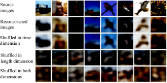
To investigate the effect of latent spiking variables, we sample a latent spiking variable $z$ by the autoregressive Bernoulli method of FSVAE. We then shuffle the spikes along the length and time dimensions respectively. Fig. 1 shows the comparison of different generated images on CIFAR10. Through this experiment, we discover the temporal robustness phenomenon: shuffling in the time dimension has negligible effect while shuffling in the length dimension significantly changes the generated images.

Further reflection on this phenomenon reveals that disrupting spikes in the time dimension does not change the firing rate of each latent variable neuron. This discovery lays the foundation for our construction of latent spaces with Poisson distributions, which will be detailed in Sec. III-A.

Figure 2: The model training and image generating processes of ESVAE.

III Methods

In this section, we propose an efficient spiking variational autoencoder (ESVAE) that uses a simpler reparameterizable Poisson sampling method. We introduce the construction of the posterior and prior distributions of the latent space in Sec. III-A. Then the proposed Poisson spiking sampling method is described in Sec. III-B. The evidence lower bound (ELBO) and loss function are derived in Sec. III-C.

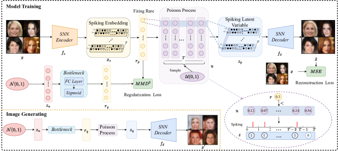
The training and image generating processes are shown in Fig. 2. The input image $x$ is fed into SNN encoder $f_{e}$ which outputs the spiking embedding $x_{e}\in\{0,1\}^{d\times T}$, where $d$ is the length dimension and $T$ is the SNN time window. Then the latent spiking variable $z_{p}\in\{0,1\}^{d\times T}$ is randomly generated by the Poisson process based on the firing rate $r_{p}\in\left\{\frac{1}{T},...,\frac{T}{T}\right\}^{d}$ of $x_{e}$. Subsequently, the latent variable $z_{p}$ is decoded by the SNN decoder $f_{d}$ and is transformed into the reconstructed image $\hat{x}$. During the random image generation process, we first randomly sample a variable $z_{n}\in\mathbb{R}^{d}$ from a normal distribution. After a bottleneck layer, $z_{n}$ is converted into the firing rate $r_{q}\in\left(0,1\right)^{d}$ which generate the latent variable $z_{q}\in\{0,1\}^{d\times T}$ by Poisson process. Finally, the generated image $x^{\prime}$ is generated by the SNN decoder.

III-A Poisson Based Posterior and Prior Distributions

As analyzed in Sec II-B, the spiking latent variables show temporal robustness for images generated by the decoder. The firing rate of each latent variable neuron has more information relative to the order of the spike firing. Therefore, we assume that each neuron of the spiking latent variable $z$ follows a Poisson distribution, which models the number of events in an interval with independent occurrences.

In the $T$ SNN time window, the probability of emitting $n$ spike in time $T$ follows the Poisson distribution as follows:

$$P\left(n\text{ spikes in }T\text{ time steps}\right)=\frac{(r\cdot T)^{n}}{n!}e^{-r\cdot T},$$ (4)

where $r$ means the expectation of the spike firing rate. We set $\lambda=r\cdot T$ to denote the intensity parameter of the Poisson distribution, meaning the expected number of spikes in time $T$.

Then, we denote the posterior probability distribution $p(z_{p}|x;r_{p})$ and the prior probability distribution as $q(z_{q};r_{q})$, where $r_{p}$ and $r_{q}$ are the expectation of the firing rate of posterior and prior, respectively; $z_{p}$ and $z_{q}$ denote the latent variables generated by posterior and prior, respectively.

The posterior $p(z_{p}|x;r_{p})$ is modeled by the SNN encoder. To project the input image into a latent Poisson distribution space, the firing rate $r_{p}$ of the encoder output $x_{e}$ is considered as the expected firing rate of the latent Poisson distribution, with the same length dimension as the spiking latent variable $z_{p}$. For instance, the firing rate $r^{i}$ of the $i^{th}$ output neuron is computed as:

$$r_{p}^{i}=\frac{1}{T}\sum_{t=1}^{T}x_{e}^{i,t}.$$ (5)

For constructing the prior $q(z_{q};r_{q})$, the distribution of $r_{q}$ is crucial, as its values encapsulate information of the generated images. Therefore, we propose using a bottleneck layer to obtain $r_{q}$ parameters of the prior which consists of a fully-connected layer and a sigmoid active function as depicted in the generating branch of Fig. 2. The bottleneck input $z_{n}$ is sampled from a normal distribution, considered the most prevalent naturally occurring distribution.

III-B Reparameterizable Poisson Spiking Sampling

For both the prior and posterior distributions, the target is making the $i^{th}$ neuron of the latent variable fire at a rate $r^{i}$. The spike-generating process is modeled as a Poisson process. Thus, the probability of the $i^{th}$ neuron firing at time $t^{th}$ is expressed as follows:

$$P\left(\text{Firing at }t^{th}\text{ time step}\right)=r^{i}.$$ (6)

Specifically, we first generate a random variable $u\in\{a|0\leqslant a\leqslant 1\}^{d\times T}$ from a uniform distribution. Then, along the time dimension, the value of $u$ is compared with the firing rate $r$ of the corresponding position to generate $z$, which is formulated by:

$$z^{i,t}=\left\{\begin{aligned} &1,u^{i,t}<r^{i},\\ &0,otherwise.\end{aligned}\right.$$ (7)

where $u^{i,t}$ and $z^{i,t}$ are the $i^{th}$ value at $t^{th}$ time step of $u$ and spiking latent variable $z$.

Since Eq. 7 is a step function, $z$ is not differentiable with respect to $r$. To reparameterize $z$, we use the surrogate gradient of our SNN training as follows:

$$\frac{\partial z^{i}}{\partial r^{i}} =\sum_{t=1}^{T}\frac{\partial z^{i,t}}{\partial r^{i}}$$ (8)

$$=\frac{1}{\alpha}\sum_{t=1}^{T}\operatorname{sign}\left(|r^{i}-u^{i,t}|<\frac{\alpha}{2}\right),$$

where $\alpha$ is the width parameter to determine the shape of gradient [17].

Algorithm 1 ESVAE Model Training and Image Generating Algorithms.

1:Training dataset $\mathcal{X}$.

2:Reconstructed images $\hat{\mathcal{X}}$, trained SNN encoder $f_{e}$ and decoder $f_{d}$, and generated images $\mathcal{X}^{\prime}$

3:Initialize the parameters of $f_{e}$ and $f_{d}$.

4:while not done do

5:     for $x$ in $\mathcal{X}$ do

6:         $x_{e}\leftarrow f_{e}(x)$

7:         Calculate the firing rate $r_{p}$ of $x_{e}$. // Eq. 5

8:         $r_{q}\leftarrow\textsc{Prior}()$

9:         $z_{p}\leftarrow\textsc{PoissonProcess}(r_{p})$

10:         $\hat{x}\leftarrow f_{d}(z_{p})$

11:         Calculate the loss $\mathcal{L}$ with $x,\hat{x},r_{p},r_{q}$. // Eq. 11

12:         Update parameters with $\nabla\mathcal{L}$.

13:     end for

14:end while

15:$x^{\prime}\leftarrow\textsc{GenerateImages}()$

16:$\mathcal{X}^{\prime}\leftarrow\mathcal{X}^{\prime}\cup x^{\prime}$

17:function GenerateImages( )

18:     $r_{q}\leftarrow\textsc{Prior}()$

19:     $z_{q}\leftarrow\textsc{PoissonProcess}(r_{q})$

20:     $x^{\prime}\leftarrow f_{d}(z_{q})$

21:     return $x^{\prime}$

22:end function

23:function Prior( )

24:     Randomly sample $z_{n}$ from $\mathcal{N}(0,1)$.

25:     $r_{q}\leftarrow Bottleneck(z_{n})$

26:     return $r_{q}$

27:end function

28:function PoissonProcess($r$)

29:     Randomly sample $u$ from $\mathcal{U}(0,1)$.

30:     $z\leftarrow\textsc{Int}(u<r)$

31:     return $z$

32:end function

III-C Evidence Lower Bound and Loss Function

The conventional evidence lower bound (ELBO) of VAE is:

$$\operatorname{ELBO}= \mathbb{E}_{z_{p}\sim p(z_{p}|x;r_{p})}\left[\log p\left(\hat{x}|z_{p}\right)\right]$$ (9)

$$-\operatorname{KL}\left(p(z_{p}|x;r_{p})||q(z_{q};r_{q})\right),$$

where $p\left(\hat{x}|z_{p}\right)$ is the probability distribution function of the reconstructed image $\hat{x}$ generated by $z_{p}\sim p(z_{p}|x;r_{p})$. The first term usually is regarded as the reconstruction loss and reflects the quality of the image reconstructed by $z_{p}$. The second term regularizes the construction of the latent space by reducing the distance between the $p(z_{p}|x;r_{p})$ and $q(z_{q};r_{q})$ distributions in order to make the model generative.

Traditional VAEs optimize the KL divergence of these two distributions, and FSVAE argues the MMD metric is more suitable for SNNs [15]. However, these metrics are based on the generated spiking latent variables $z_{p}$ and $z_{q}$. For our ESVAE model, the difference in the spike order of $z_{p}$ and $z_{q}$ is not important, and constraining to reduce their distance will instead make training more difficult.

Therefore, we directly compute the MMD distance between the distribution $p(r_{p})$ and $q(r_{q})$ of the expected firing rate parameters $r_{p}$ and $r_{q}$. It is formulated by:

$$\operatorname{MMD}^{2}\left(p(r_{p}),q(r_{q})\right)= \mathbb{E}_{r_{p},r^{\prime}_{p}\sim p(r_{p})}\left[k\left(r_{p},r^{\prime}_{p}\right)\right]$$ (10)

$$+\mathbb{E}_{r_{p},r^{\prime}_{p}\sim q(r_{q})}\left[k\left(r_{q},r^{\prime}_{q}\right)\right]$$

$$-2\mathbb{E}_{r_{p}\sim p(r_{p}),r_{q}\sim q(r_{q})}\left[k\left(r_{p},r_{q}\right)\right],$$

where $k\left(\cdot,\cdot\right)$ is the kernel function and is set to the radial basis function (RBF) kernel in this paper.

The final loss function $\mathcal{L}$ is derived as follows:

$$\mathcal{L} =\mathbb{E}_{z_{p}\sim p(z_{p}|x;r_{p})}\left[\log p\left(\hat{x}|z_{p}\right)\right]$$ (11)

$$+\lambda\operatorname{MMD}^{2}\left(p(r_{p}),q(r_{q})\right),$$

where $\lambda$ is a hyperparameter coefficient, and the empirical estimation of $\mathbb{E}_{z_{p}\sim p(z_{p}|x;r_{p})}\left[\log p\left(\hat{x}|z_{p}\right)\right]$ is calculated by $\operatorname{MSE}(x,\hat{x})$.

The whole model training and image generating process is reported in Algorithm 1.

Dataset	Model	Model Type	Reconstruction Loss $\searrow$	Inception Score $\nearrow$	Frechet Distance $\searrow$
					Inception (FID)	Autoencoder (FAD)
MNIST	SWGAN [19]	SNN GAN	-	-	100.29	-
	SGAD [19]		-	-	69.64	-
	ANN (Kamata et al. 2022)	SNN VAE	0.048	5.947	112.5	17.09
	FSVAE (Kamata et al. 2022)		0.031	6.209	97.06	35.54
	ESVAE (Ours)		0.013	5.612	117.8	10.99
Fashion MNIST	SWGAN [19]	SNN GAN	-	-	175.34	-
	SGAD [19]		-	-	165.42	-
	ANN [15]	SNN VAE	0.050	4.252	123.7	18.08
	FSVAE [15]		0.031	4.551	90.12	15.75
	ESVAE (Ours)		0.019	6.227	125.3	11.13
CIFAR10	SWGAN [19]	SNN GAN	-	-	178.40	-
	SGAD [19]		-	-	181.50	-
	ANN [15]	SNN VAE	0.105	2.591	229.6	196.9
	FSVAE [15]		0.066	2.945	175.5	133.9
	TAID [16]		-	3.53	171.1	120.5
	ESVAE (Ours)		0.045	3.758	127.0	14.74
CelebA	SWGAN [19]	SNN GAN	-	-	238.42	-
	SGAD [19]		-	-	151.36	-
	ANN [15]	SNN VAE	0.059	3.231	92.53	156.9
	FSVAE [15]		0.051	3.697	101.6	112.9
	TAID [16]		-	4.31	99.54	105.3
	ESVAE (Ours)		0.034	3.868	85.33	51.93

TABLE I: Performance verification results on different datasets. Our model achieves state-of-the-art performance in most evaluation metrics and has a significant improvement compared with FSVAE.

IV Experiment

IV-A Datasets

MNIST [20] and Fashion MNIST [21] both have 60,000 training images and 10,000 testing images. CIFAR10 [22] consists of 50,000 images for training and 10,000 images for testing. For MNIST, Fashion MNIST, and CIFAR10, each image is resized to $32\times 32$. CelebA [23] is a classic face dataset containing 162,770 training samples and 19,962 testing samples. We resize the images of CelebA to $64\times 64$.

IV-B Implementation Details

IV-B1 Network Architecture

Following [15], we use four conventional layers to construct the backbone of the encoder and decoder on MNIST, Fashion MNIST, and CIFAR10. The detail of the structure is $32\text{C}3$-$64\text{C}3$-$128\text{C}3$-$256\text{C}3$-$128\text{FC}$-$128(\text{sampling})$-$128\text{FC}$-$256\text{C}3$-$128\text{C}3$-$64\text{C}3$-$32\text{C}3$-$32\text{C}3$-$image\_channel\text{C}3$, where 128 is the latent variable length dimension. The tdBN [24] is inserted in each layer. For CelebA, we add a $512\text{C}3$ conventional layer in the encoder following $256\text{C}3$ and also in the decoder. The bottleneck layer consists of a $128\text{FC}$ layer and the Sigmoid active function.

IV-B2 Training Setting

For the SNN, we set the time window $T$ to 16, the firing threshold $v_{\theta}$ to 0.2, the membrane potential decay factor $\tau$ to 0.25; the width parameter $\alpha$ of the surrogate gradient to 0.5. The model is trained 300 epochs by AdamW optimizer with 0.0006 learning rate and 0.001 weight decay. The learning rate on the bottleneck layer is set to 0.006.

IV-B3 Hardware Platform

The source code is written with the Pytorch framework [25] on Ubuntu 16.04 LTS. All the models are trained using one NVIDIA GeForce RTX 2080Ti GPU and Intel Xeon Silver 4116 CPU.

IV-C Performance Verification

In this section, we compare our ESVAE with state-of-the-art SNN VAE methods FSVAE (including the ANN version) [15] and TAID [16]. FSVAE is the first fully SNN VAE model which is reported at AAAI22. TAID adds an attention mechanism based on FSVAE to further improve the performance, without the different latent space construction and sampling method, published in ICLR23. In addition, we also compare the quality of the generated images with the SNN GAN model.

Table I shows the comparison results of different evaluation metrics on each dataset, in which the reconstruction loss, inception score [26] and FID [27] are the commonly used metrics to measure the generated images. FAD is proposed by [15] to measure the distribution distance between generated and real images.

For the reconstruction loss, our method achieves the lowest loss on both four datasets. For the generation metrics, the proposed ESVAE also achieves the best results in most items. It is worth noting that ESVAE gets much better scores on FAD than the other methods. This means that the posterior distribution $p(z_{p}|x;r_{p})$ constructed explicitly can better project the distribution of the training images. The experimental results indicate that our method well balances the ability of image restoration and generation.

Figure 3: Generated images of SGAD, FSAVE, TAID, and the proposed ESVAE on CIFAR10 and CelebA.

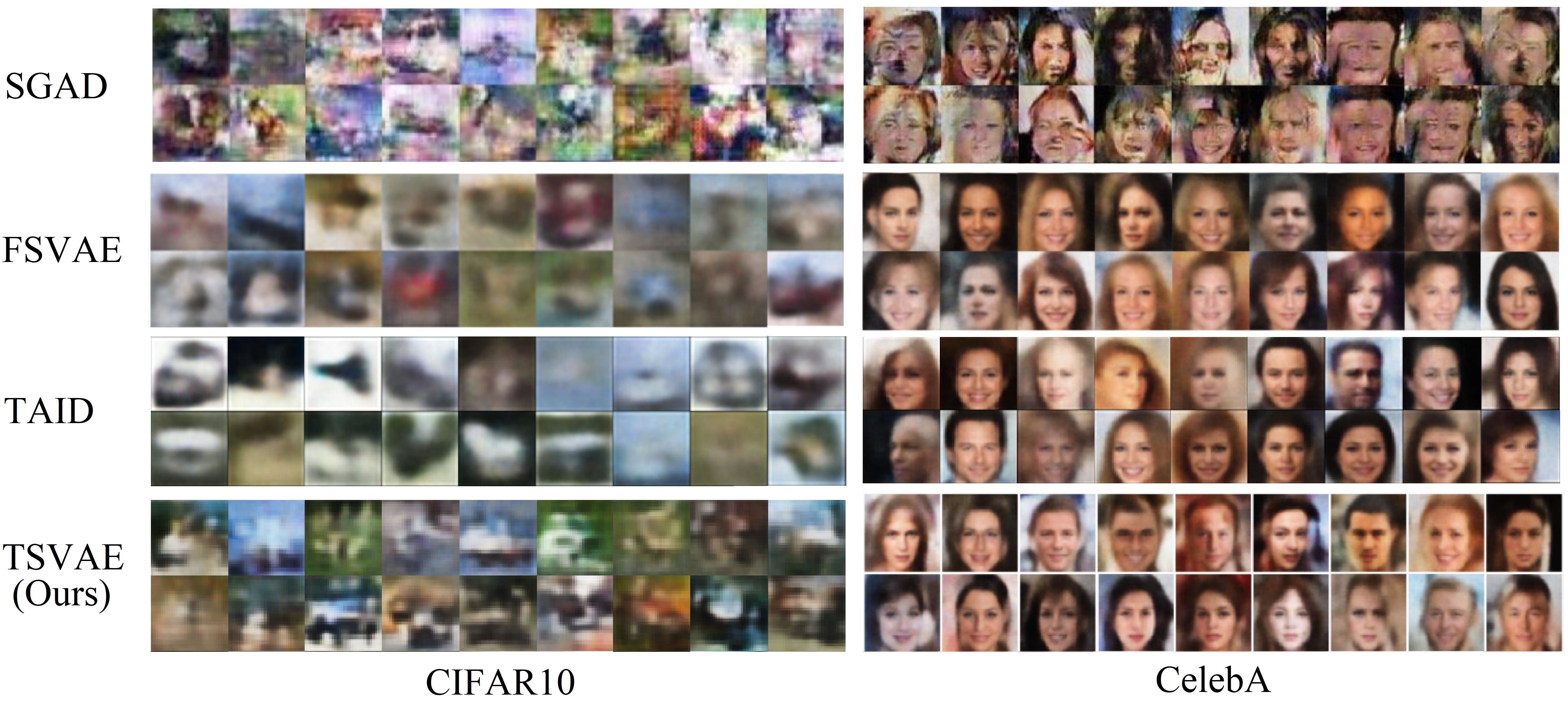
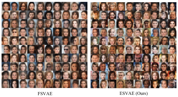
Fig. 3 shows the generated images by SGAD, FSVAE, TAID, and ESVAE on CIFAR10 and CelebA. Compared with other SNN VAE methods, ESVAE generates images with more details instead of blurred pixels with similar colors. This is attributed to the better balance between image reduction and generation capabilities in the ESVAE model. It is worth noting that the images generated by the SNN GAN method SGAD have richer colors and more diverse details. However, these images lack sufficient rationality, which may be caused by the difficulty of GAN training.

More reconstructed and generated image comparisons are shown in Appendix A and B.

IV-D Robustness Analysis

IV-D1 Temporal Robustness

We apply the same method as in Section II-B to shuffle the latent variables along time dimensions and generate new images. To compare the temporal robustness accurately, we quantitatively analyze it by calculating the reconstruction loss between images.

As shown in Table II, our method has the strongest temporal robustness in comparison with both original and vanilla reconstructed images. This property makes our method more resistant to problems such as firing delays or confusion arising in hardware.

Dataset	Model	vs. Original Image	vs. Vanilla Reconstructed Image
MNIST	FSVAE	0.0270	0.0074
	ESVAE	0.0105	0.0021
Fashion MNIST	FSVAE	0.0529	0.0265
	ESVAE	0.0169	0.0030
CIFAR10	FSVAE	0.0707	0.0060
	ESVAE	0.0434	0.0031
CelebA	FSVAE	0.0553	0.0099
	ESVAE	0.0330	0.0037

TABLE II: The reconstruction loss of images generated by time-shuffled variables versus original and vanilla reconstructed images.

To further analyze the reason for the better temporal robustness, we visualize the spiking latent variables of CelebA shown in Fig. 4. Observation of the spike trains of each neuron reveals that these neurons have relatively extreme firing characteristics: either high or low firing rates. This phenomenon is even more pronounced in ESVAE, where many neurons either fire all or not at all. This feature makes the order of each neuron’s spike firing have limited influence on the final generated image. This indicates that the multivariate distribution of the latent space is not obtained by the independent merging of the distributions of different neurons, and the combination order of neurons with different firing rates is also one of the important elements of the distribution of the latent space.

Figure 4: The latent variables sampled by FSVAE and ESVAE on CelebA at the training and generating stage. The horizontal axis is the length dimension of the variable, and the vertical axis is the time dimension.

IV-D2 Gaussian Noise Robustness

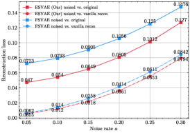
To evaluate the robustness more comprehensively, we add Gaussian noise to the spiking latent variables with probability $a$ on CIFAR10, so that some of the existing spikes disappear or new spikes appear. As with the test of temporal robustness, we quantify the analysis by calculating the reconstruction loss with the original images and vanilla reconstructed images. Similarly to the temporal robustness analysis, robustness is quantified by the reconstruction loss between original images and vanilla reconstructed images without noise.

Fig. 5 shows the reconstruction loss curves of images generated by noised latent variables. The experimental results demonstrate that ESVAE is more robust to noise, both in comparison with the original images and with the vanilla reconstructed images.

The images generated by noised latent variables are shown in Appendix C.

Figure 5: The reconstruction loss curves of noise robustness on CIFAR10. Red lines are the curves of ESVAE and blue are of FSVAE. Solid and dashed lines show the losses calculated with original images and vanilla reconstructed images, respectively.

IV-E Comparison of Encoder on Classification Task

The powerful image generation capabilities and robustness of ESVAE demonstrated in Sec. IV-C and IV-D are mainly brought by the SNN decoder. We now analyze the capabilities of the encoder by classifying the encoder embeddings $x_{e}$. We feed the firing rate $r_{p}$ of $x_{e}$ into an ANN classifier which consists of four fully connected layers: $128$-$512\text{FC}$-$256\text{FC}$-$128\text{FC}$-$10\text{FC}$.

	CIFAR10	Fashion MNIST	MNIST
FSVAE	46.65	86.28	98.00
ESVAE	53.59	88.59	98.09

TABLE III: The classification accuracies (%) of encoder output.

The classifier is trained 200 epochs by an SGD optimizer with a 0.01 learning rate on the training set. Table III shows the test accuracy on CIFAR10, Fashion MNIST, and MNIST. The results show that ESVAE achieves the highest classification accuracy on all datasets. Especially on CIFAR10, the accuracy of ESVAE is 6.94% higher than FSVAE, which indicates that our encoder preserves more information about the input image on the complex dataset.

IV-F Comparison on Distribution Consistency

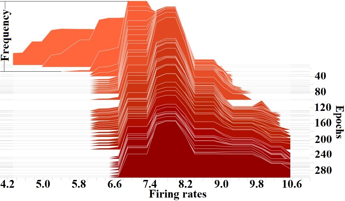
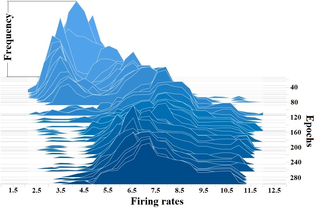
In this section, we analyze the posterior and prior distribution consistency between training and generating stages, by visualizing the frequency of the firing rate in all neurons of latent variables. The visualization results are shown in Fig. 6. For the distribution of mean firing rates, the overlap between the training and generating stages is high on both ESVAE Fig. 6(b) and FSVAE Fig. 6(a). This suggests that the distance of the distributions can also be effectively reduced by optimizing the MMD loss between firing rates.

(a) Mean firing rates of FSVAE.

(b) Mean firing rates of ESVAE.

(c) Single sample firing rates of FSVAE.

(d) Single sample firing rates of ESVAE.

Figure 6: The firing rate distribution of FSVAE and ESVAE on the CIFAR10 dataset. Fig. 6(a) and 6(b) are the mean firing rate distribution of all the generated images. Fig. 6(c) and 6(d) are the firing rate distribution of a single image generated by FSVAE and ESVAE respectively.

(a) FSVAE training.

(b) ESVAE training.

(c) FSVAE generating.

(d) ESVAE generating.

Figure 7: Firing rates distributions of FSVAE and ESVAE at different training epochs on CIFAR10. The horizontal axis represents the firing rate, while the vertical axis depicts frequency. Different colors represent different training epochs.

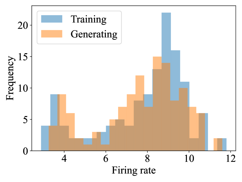
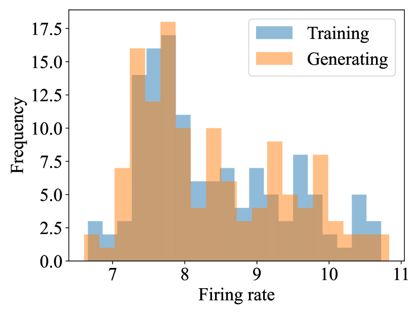
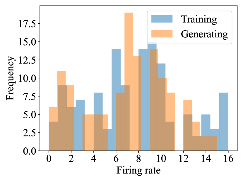
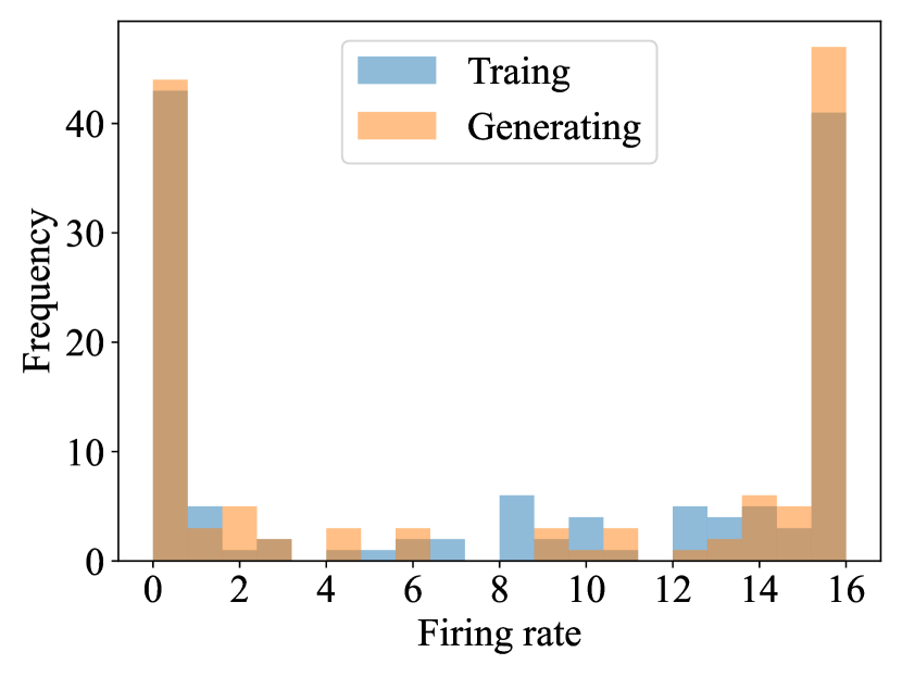
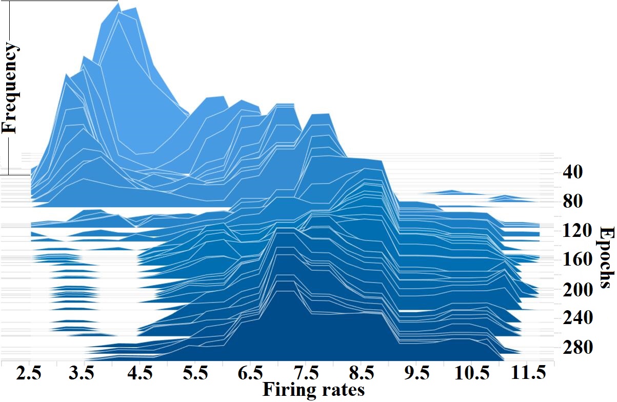
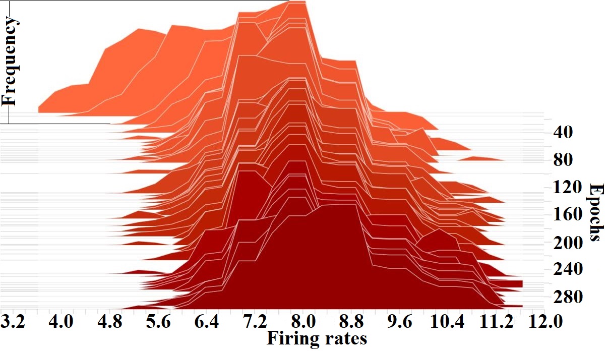
Another interesting observation is that the distribution of a single generated image, as shown in Fig. 6(d), is far from the mean firing rate distribution. The distribution shown in Fig. 6(c) is also not the same as the mean firing rate distribution of FSVAE, but the gap is smaller than that of ESVAE. We believe that this difference is brought about by the distinction between the different categories of samples. In ESVAE, the difference between the distribution of individual samples and the mean distribution is greater, which also suggests a higher distinction between the samples. The better classification ability shown in Table III can also prove this conclusion.

Fig. 7 shows the distribution changes of FSVAE and ESVAE during training and generating processes. The firing rate distribution of ESVAE training converges faster than FSVAE. The distribution shape of ESVAE training remains largely consistent in early training, with the generating distribution closely matching it. The distribution of FSVAE generating is also in high consistency with the training distribution, yet it takes more training epochs to converge to a stable distribution shape.

V Conclusion

In this paper, we propose an ESVAE model with reparameterizable Poisson spiking sampling method. The latent space in SNN is explicitly constructed by a Poisson-based posterior and prior distribution, which improves the interpretability and performance of the model. Subsequently, the proposed sampling method is used to generate the spiking latent variables by the Poisson process, and the surrogate gradient mechanism is introduced to reparameterize the sampling method. We conduct comprehensive experiments on benchmark datasets. Experimental results show that images generated by ESVAE outperform the existing SNN VAE and SNN GAN models. Moreover, ESVAE has stronger robustness, a higher distribution consistency, as well as an encoder with more information retention. In the future, we will try to explore the SNN VAE method suitable for event data recorded by neuromorphic cameras to expand the practice of SNNs.

Appendix A Reconstructed Images

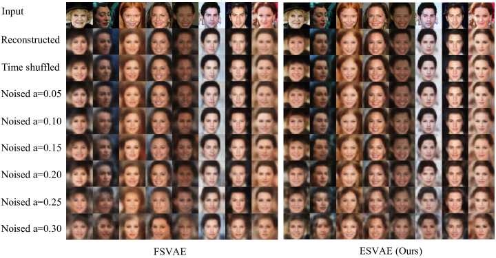
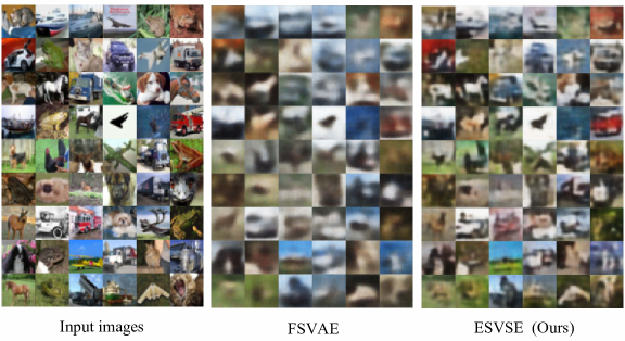
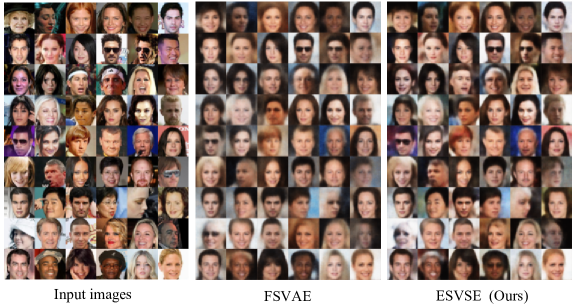
Fig. 8 and 9 compare reconstructed images of FSVAE [15] and ESVAE on CIFAR10 and CelebA, respectively. Our ESVAE demonstrates a higher-quality reconstruction with more image detail than the fuzzy blocks of color demonstrated by FSVAE.

Figure 8: Reconstructed images of FSAVE and ESVAE on CIFAR10.

Figure 9: Reconstructed images of FSAVE and ESVAE on CelebA.

Appendix B Generated Images

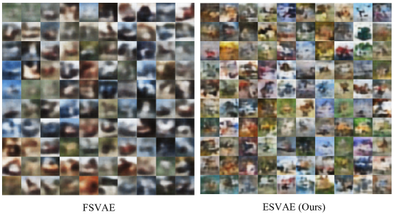
The randomly generated images of FSVAE and ESVAE are shown in Fig. 10 and 11, respectively. As reconstructed images, generated images of ESVAE have richer color variations.

Figure 10: Generated images of FSAVE and ESVAE on CIFAR10.

Figure 11: Generated images of FSAVE and ESVAE on CelebA.

Appendix C Noised Images

Fig. 12 and 13 illustrate the images generated by the latent variables with different noise disturbances on CIFAR10 and CelebA, respectively. For ESVAE, disrupting the spike order of the latent variables, the generated images are almost no different from the vanilla reconstructed images. Under Gaussian noise interference, it can be seen that when $a$ reaches 0.1, the images generated by FSVAE are more different from the variables reconstructed images, while ESVAE still maintains the distinctive features of the original images to a greater extent.

Figure 12: Noised images of FSAVE and ESVAE on CIFAR10.

Figure 13: Noised images of FSAVE and ESVAE on CelebA.

References

- [1] C. Zhang, C. Zhang, S. Zheng, Y. Qiao, C. Li, M. Zhang, S. K. Dam, C. M. Thwal, Y. L. Tun, L. L. Huy et al., “A complete survey on generative ai (aigc): Is chatgpt from gpt-4 to gpt-5 all you need?” arXiv preprint arXiv:2303.11717, 2023.
- [2] D. P. Kingma and M. Welling, “Auto-encoding variational bayes,” arXiv preprint arXiv:1312.6114, 2013.
- [3] M.-H. Yu, J. Li, D. Liu, D. Zhao, R. Yan, B. Tang, and H. Zhang, “Draft and edit: Automatic storytelling through multi-pass hierarchical conditional variational autoencoder,” in Proceedings of the AAAI Conference on Artificial Intelligence, vol. 34, no. 02, 2020, pp. 1741–1748.
- [4] F. Ye and A. G. Bors, “Continual variational autoencoder via continual generative knowledge distillation,” in Proceedings of the AAAI Conference on Artificial Intelligence, vol. 37, no. 9, 2023, pp. 10 918–10 926.
- [5] M. Xu, H. Du, D. Niyato, J. Kang, Z. Xiong, S. Mao, Z. Han, A. Jamalipour, D. I. Kim, V. Leung et al., “Unleashing the power of edge-cloud generative ai in mobile networks: A survey of aigc services,” arXiv preprint arXiv:2303.16129, 2023.
- [6] W. Maass, “Networks of spiking neurons: the third generation of neural network models,” Neural networks, vol. 10, no. 9, pp. 1659–1671, 1997.
- [7] Q. Zhan, G. Liu, X. Xie, M. Zhang, and G. Sun, “Bio-inspired active learning method in spiking neural network,” Knowledge-Based Systems, p. 110193, 2022.
- [8] G. Liu, W. Deng, X. Xie, L. Huang, and H. Tang, “Human-level control through directly trained deep spiking -networks,” IEEE Transactions on Cybernetics, 2022.
- [9] M. Davies, N. Srinivasa, T.-H. Lin, G. Chinya, Y. Cao, S. H. Choday, G. Dimou, P. Joshi, N. Imam, S. Jain et al., “Loihi: A neuromorphic manycore processor with on-chip learning,” Ieee Micro, vol. 38, no. 1, pp. 82–99, 2018.
- [10] M. V. DeBole, B. Taba, A. Amir, F. Akopyan, A. Andreopoulos, W. P. Risk, J. Kusnitz, C. O. Otero, T. K. Nayak, R. Appuswamy et al., “Truenorth: Accelerating from zero to 64 million neurons in 10 years,” Computer, vol. 52, no. 5, pp. 20–29, 2019.
- [11] J. Pei, L. Deng, S. Song, M. Zhao, Y. Zhang, S. Wu, G. Wang, Z. Zou, Z. Wu, W. He et al., “Towards artificial general intelligence with hybrid tianjic chip architecture,” Nature, vol. 572, no. 7767, pp. 106–111, 2019.
- [12] N. Skatchkovsky, O. Simeone, and H. Jang, “Learning to time-decode in spiking neural networks through the information bottleneck,” Advances in Neural Information Processing Systems, vol. 34, pp. 17 049–17 059, 2021.
- [13] K. Stewart, A. Danielescu, T. Shea, and E. Neftci, “Encoding event-based data with a hybrid snn guided variational auto-encoder in neuromorphic hardware,” in Proceedings of the 2022 Annual Neuro-Inspired Computational Elements Conference, 2022, pp. 88–97.
- [14] S. Talafha, B. Rekabdar, C. Mousas, and C. Ekenna, “Biologically inspired sleep algorithm for variational auto-encoders,” in Advances in Visual Computing: 15th International Symposium, ISVC 2020, San Diego, CA, USA, October 5–7, 2020, Proceedings, Part I 15. Springer, 2020, pp. 54–67.
- [15] H. Kamata, Y. Mukuta, and T. Harada, “Fully spiking variational autoencoder,” in Proceedings of the AAAI Conference on Artificial Intelligence, vol. 36, no. 6, 2022, pp. 7059–7067.
- [16] X. Qiu, Z. Luan, Z. Wang, and R.-J. Zhu, “When spiking neural networks meet temporal attention image decoding and adaptive spiking neuron,” 2023. [Online]. Available: https://openreview.net/forum?id=MuOFB0LQKcy
- [17] Y. Wu, L. Deng, G. Li, J. Zhu, Y. Xie, and L. Shi, “Direct training for spiking neural networks: Faster, larger, better,” in Proceedings of the AAAI conference on artificial intelligence, vol. 33, no. 01, 2019, pp. 1311–1318.
- [18] X. Xie, B. Yu, G. Liu, Q. Zhan, and H. Tang, “Effective active learning method for spiking neural networks,” IEEE Transactions on Neural Networks and Learning Systems, 2023.
- [19] L. Feng, D. Zhao, and Y. Zeng, “Spiking generative adversarial network with attention scoring decoding.” CoRR, 2023.
- [20] L. Deng, “The mnist database of handwritten digit images for machine learning research [best of the web],” IEEE signal processing magazine, vol. 29, no. 6, pp. 141–142, 2012.
- [21] H. Xiao, K. Rasul, and R. Vollgraf, “Fashion-mnist: a novel image dataset for benchmarking machine learning algorithms,” arXiv preprint arXiv:1708.07747, 2017.
- [22] A. Krizhevsky et al., “Learning multiple layers of features from tiny images,” 2009.
- [23] Z. Liu, P. Luo, X. Wang, and X. Tang, “Large-scale celebfaces attributes (celeba) dataset,” Retrieved August, vol. 15, no. 2018, p. 11, 2018.
- [24] H. Zheng, Y. Wu, L. Deng, Y. Hu, and G. Li, “Going deeper with directly-trained larger spiking neural networks,” in Proceedings of the AAAI conference on artificial intelligence, vol. 35, no. 12, 2021, pp. 11 062–11 070.
- [25] A. Paszke, S. Gross, F. Massa, A. Lerer, J. Bradbury, G. Chanan, T. Killeen, Z. Lin, N. Gimelshein, L. Antiga et al., “Pytorch: An imperative style, high-performance deep learning library,” Advances in neural information processing systems, vol. 32, 2019.
- [26] T. Salimans, I. Goodfellow, W. Zaremba, V. Cheung, A. Radford, and X. Chen, “Improved techniques for training gans,” Advances in neural information processing systems, vol. 29, 2016.
- [27] M. Heusel, H. Ramsauer, T. Unterthiner, B. Nessler, and S. Hochreiter, “Gans trained by a two time-scale update rule converge to a local nash equilibrium,” Advances in neural information processing systems, vol. 30, 2017.